Assessing the liquefaction potential of seabed soils based on ocean ambient noise in the Yellow River Delta

Seabed soils can undergo liquefaction under cyclic loading, resulting in a rapid decrease in strength and stiffness, which may lead to the destruction of offshore structures. Therefore, the assessment of seabed soil liquefaction will become an important factor in disaster prevention and risk analysis in coastal and offshore engineering construction. In this study, the ocean ambient noise with low-frequency, long-wavelength, and wide-band characteristics was used to conduct and analysis noise based on the horizontal-to-vertical spectral ratio method. The shear wave velocity of the seabed soil was obtained by inverting the ocean ambient noise dataset. Then, we proposed a shear wave velocity threshold that can be used for liquefaction assessment of Holocene unconsolidated fine-grained soils by statistical analysis, and the liquefaction potential of the soils was evaluated according to 1-D shear wave velocity structures and 2-D shear wave velocity profiles. The results showed that the distribution of the shear wave velocity obtained by inverting ocean ambient noise was generally consistent with the measured shear wave velocity in the field, indicating that the inversion results have a certain degree of accuracy. A shear wave velocity threshold of 200 m/s was proposed for liquefaction assessment, determining that the soils within 0-10 m depth in the coastal area of Yellow River Delta have liquefaction potential. This result is in accordance with the assessment based on the critical shear wave velocity, indicating that this threshold is applicable to the assessment of seabed soil liquefaction in the Yellow River Delta. The in-situ observations of ocean ambient noise provide a more convenient, economical, and environmentally friendly method, which can help to investigate marine geology disasters and serve marine engineering construction.

1 Introduction

Soil liquefaction is one of the significant factors affecting soil stability, among them, seabed soil liquefaction is a harmful marine geological disaster, which has attracted widespread attention from domestic and foreign geotechnical engineering and coastal engineering communities. Under the continuous erosion and scouring of waves, fine particles on the surface soil of the seabed migrate out and escape along the pores of the coarse particles, thereby forming larger pores in the soil (Dassanayake et al., 2022). This can destroy the structural integrity of the soil, and weaken the hydraulic properties (Jia et al., 2014) and engineering characteristics (Liu et al., 2013) of the soil, which may induce soil liquefaction under cyclic loading (Bachrach et al., 2001), causing damage to offshore structures such as submarine pipelines (Sumer et al., 1999; Zhou et al., 2013), offshore platforms (Sumer, 2014; Zhang et al., 2017), and breakwaters (Jeng, 2001; Zhao and Jeng, 2015). The Yellow River Delta is a typical rapidly deposited delta, and also the place with the densest offshore structures on the south coast of the Bohai Bay. The fine-grained soils such as silt and silty sand are widely developed in the Yellow River Delta, with weaker permeability and poorer water stability, which makes them more prone to unstable failure of soil such as liquefaction (Ren et al., 2020; Wang et al., 2022; Liu et al., 2023; Zhang et al., 2023). For this reason, accurately assessing the seabed liquefaction has become an essential part of disaster prevention and mitigation in the construction of the Yellow River Delta.

At present, there are three primary methods for assessing soil liquefaction: in-situ tests (Fergany and Omar, 2017), laboratory tests (Kumar et al., 2020), and numerical simulation (Ye et al., 2016; Zhao et al., 2018). These methods have been maturely applied in the study of liquefaction in sandy soils due to their safety and reliability (Amini and Qi, 2000; Dobry and Abdoun, 2017; Ye et al., 2018). However, for seabed soil, sampling measurements and laboratory tests can only obtain the physical and mechanical properties of shallow soil layers (Meng et al., 2018), and cannot guarantee the natural structure and stress state of seabed soil, resulting in failure to reflect the real dynamic response of soil. Numerical simulation can provide guidance for experimental research and theoretical analysis, but the simplification of boundary conditions and material properties in the numerical simulation process with a certain degree of randomness can lead to affect the reliability of the results. Furthermore, invasive in-situ tests such as standard penetration test (SPT) (Seed et al., 1983) and cone penetration test (CPT) (Boumpoulis et al., 2021; Geyin and Maurer, 2021) are complex and expensive, making them unsuitable for large-scale seabed measurements. Submarine acoustic exploration technology uses the acoustic properties of the compression waves (P-waves) and the shear waves (S-waves) to investigate the engineering properties of seabed soils. This method can effectively avoid measuring errors caused by disturbances, which is becoming a prominent means for studying the properties of seabed soils (Gorgas et al., 2002; Hou et al., 2018). Compared with the results of SPT and CPT testing, shear wave velocity (V_s) is closely related to liquefaction resistance, and is influenced by factors such as porosity ratio, stress state, relative density, and soil type (Hardin and Drnevich, 1972; Tokimatsu and Uchida, 1990; Xu et al., 2015). Moreover, V_s is one of the fundamental mechanical properties of soils, which can characterize the shear stiffness under small strain conditions and soil-structure interaction, and has potential application prospects in assessing soil liquefaction (Qin et al., 2020; Lin et al., 2021). Nevertheless, traditional shear wave velocity testing requires placing shear wave sensors in surface or underground boreholes, making it difficult to conduct measurements in the seabed. Moreover, the harsh seafloor environment and complex sediment structure seriously affect the measurement accuracy, and the high cost and limited measurement range restrict the development of submarine acoustic exploration technology.

There exist weak and low-amplitude vibration in the natural environment, known as ambient noise, which are commonly considered as an interference signal in geophysics. Over the past few decades, researchers have gradually discovered that ambient noise can be used to prospect subsurface structures (Aki, 1957; Toksoz, 1964). The composition of different body and surface waves in ambient noise is highly complex (Bonnefoy-Claudet et al., 2006). Nakamura (Nakamura, 1989; Nakamura, 2008; Nakamura, 2009) proposed the horizontal to vertical spectral ratio method (HVSR), which normalizes the amplification effects of the horizontal and vertical components of ambient noise, calculates the Fourier spectrum ratio of the horizontal and vertical components of noise, and evaluates the ground response characteristics of soft sediment caused by multiple reflections of shear waves (Nakamura, 2000; Nakamura, 2019). The HVSR curve is closely related to the properties of the soil (Field et al., 1990; Field and Jacob, 1993) and is considered as a “transfer function” of the vertically incident shear wave in the strata (Nakamura, 1989; Nakamura, 2008). Kawase et al. (2011) proved that the horizontal-to-vertical spectral ratios match the ratios estimated from 1D shear wave velocity model using the simple theory of diffuse field. Therefore, based on the fundamental resonant frequency and spectral amplitude on the HVSR curve, the shear wave velocity can be estimated using an inversion algorithm (forward modeling routine and Monte Carlo method) and an empirical relationship between shear wave velocity and depth, such as the quarter-wavelength theory (Joyner et al., 1981; Boore, 2003; Edwards et al., 2011). The ambient noise on land is mainly caused by industrial machinery, vehicles, and other human activities, which is predominantly composed of high-frequency and short-wavelength noise (Bonnefoy-Claudet et al., 2006). In contrast, ocean ambient noise is mainly caused by the action of waves on the seabed (Hasselmann, 1963; Bromirski et al., 2005), and it is a broad-band vibration with low-frequency and long-wavelength characteristics, which ensures that ocean ambient noise exploration has a greater detection depth and sufficient resolution.yao

The structure of this study is as follows: Firstly, we introduce the feasibility analysis for assessing the liquefaction potential of seabed soils based on shear wave velocities obtained by inverting ocean ambient noise. Secondly, we present the geological overview of the study area (the coastal zone of the Yellow River Delta). Third, we describe the inversion method and strategy of ocean ambient noise. Fourth, we discuss the characteristics of ocean ambient noise and the accuracy of inversion results, respectively. In addition, we propose and validate the shear wave velocity threshold that can be used for fine-grained soil liquefaction assessment based on statistical analysis. Finally, we conclude this study by discussing and concluding the effectiveness, limitations and potential for assessing the liquefaction of seabed soils by the shear wave velocity obtained by the inversion of ocean ambient noise.

2 Geological overview

The Yellow River Delta is located on the southern coast of Bohai, and the Yellow River Delta Plain is a fluvial plain formed by the long-term siltation and continuous sea reclamation of high-concentration sediment carried by the Yellow River. We selected the northern coastal zone of the Yellow River Delta as our study area (Figure 1), which has an overall flat topography and gentle slope. The thickness of the Quaternary strata is about 26 m, with a horizontal distribution. Due to the special deposition pattern, silty soils are commonly developed in the surface sediments, with predominantly silt, fine sand and small amounts of clay (Zhao et al., 2013), showing the engineering characteristics of a high water content, poor grading, low bearing capacity, and high compressibility. In addition, thin-layered soft soil layers are widely developed in the stratum, with a thickness of about 1-5 m, which are interspersed with the sedimentary layers in a finger-like way. The engineering geological environment of the Yellow River Delta region is controlled by the sedimentary dynamic environment, which is mainly determined by the muddy and sandy nature of the Yellow River and its frequent siltation and migration. Owing to the migration of the Yellow River Estuary, the sediment supply has been interrupted. In the northern coastal zone, under the action of long-term differential hydrodynamic forces, the structural integrity of the surface soil of the tidal flats are destroyed, leading to a decrease in strength and gradual erosion, which has formed a drop of nearly 1 m between the tidal flats and the embankment. Thus, the study of the engineering characteristics of seabed soil under dynamic action would be helpful to maintain the safety of marine buildings.

FIGURE 1

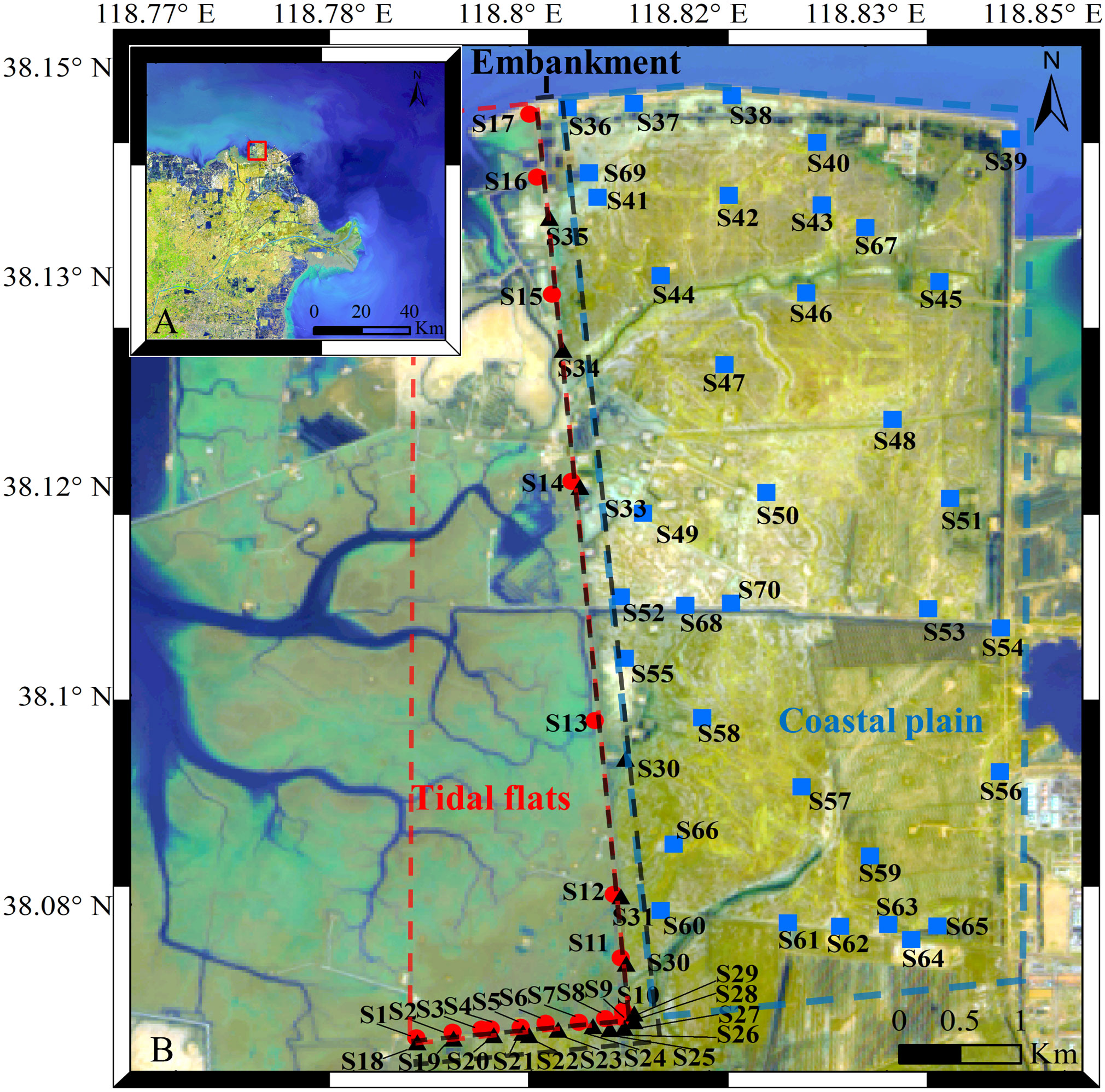
Figure 1 Map of the northern coastal areas of the Yellow River Delta. (A) The map of the study area (red rectangle). (B) The distribution of measurement stations within the study area. The red dashed line represents the tidal flats with the stations in red circles; the black dashed line represents the embankment with the stations in black triangles; the blue dashed line represents the coastal plain with the stations in blue square.

3 Inversion method

In this paper, the OpenHVSR-inversion program (Bignardi et al., 2018) is used to invert the HVSR curves of ocean ambient noise and obtain the shear wave velocity. This program can be used to model and invert HVSR dataset simultaneously, obtaining the distribution of shear wave velocity in different depth layers to construct 2-D or 3-D subsurface models. The forward modeling is based on the method proposed by Tsai and Housner (1970), which calculates the theoretical transfer function of the layered subsurface model. The inversion strategy is based on the Monte Carlo method, where a randomly perturbed version of the best fitting model is generated in each iteration, and used to compute a set of simulated curves for comparison with experimental curves. The generation of many trial models allows exploring the parameters space while searching for a new and better fitting model.

Several in-situ ambient noise recordings were carried out in the Yellow River Delta, and the observed distribution of fundamental frequency is shown in Figure 2, which is mainly concentrated in the range of 0.8-9.8 Hz (Meng et al., 2023). As a result, we set the frequency band for inversion from 0.6 to10 Hz. The inversion was divided into three stages. In the first stage, the inversion was started with a simple 4-layer subsurface model (Table 1), limiting the frequency band to 0.6-4 Hz. Successively, when the best-fit model was found, the result was saved as a new project and the subsurface model was edited, dividing the deeper layer in three sublayers, while the total thickness of the layer remains unchanged. Then, set the frequency band for the second stage to 0.6-8 Hz and continue with the next, with the shallower layer dividing in four sublayers, and so on. The frequency band for the third stage was set at 0.6-10 Hz, with a total of 10 layers.

FIGURE 2

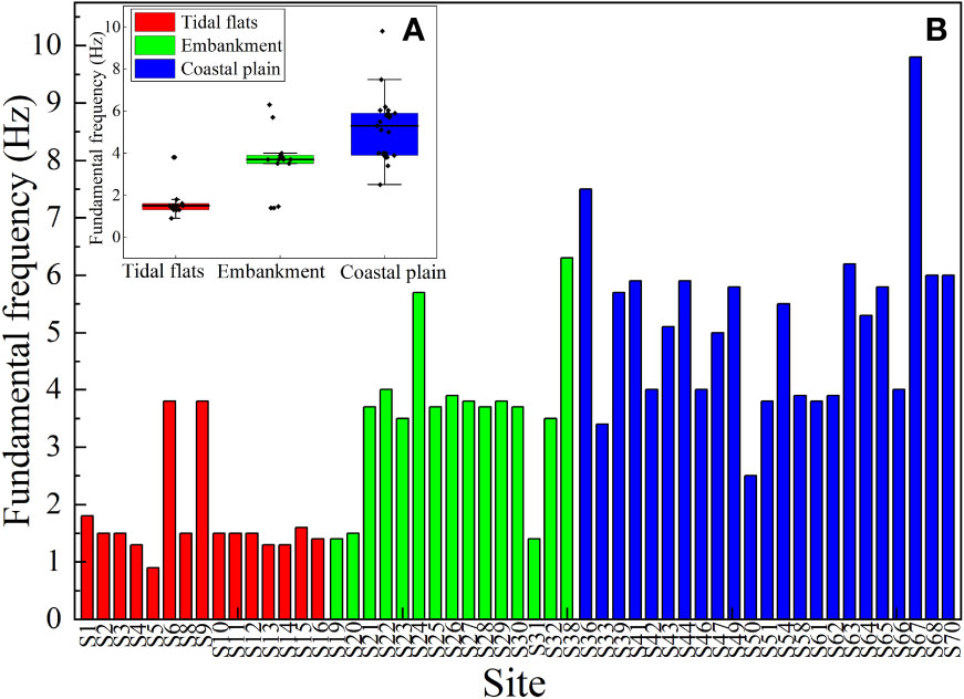
Figure 2 Statistics of fundamental frequency in the coastal zone of the Yellow River Delta (modified from Meng et al., 2023). (A) The distribution of fundamental frequency for stations in different study areas, where the red represents the tidal flats, the green represents the embankment, and the blue represents the coastal plain. (B) The fundamental frequency for all stations.

TABLE 1

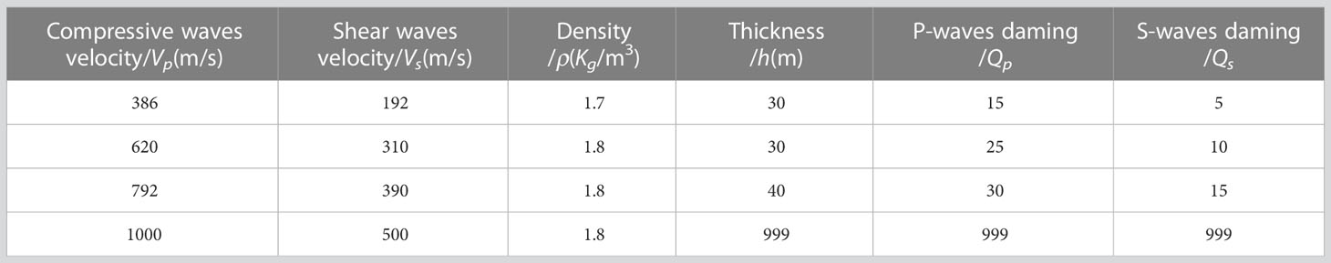
Table 1 Initial subsurface parametric model.

In each stage of the inversion, firstly, the longitudinal wave velocity, shear wave velocity, and thickness were allowed a 5% perturbation for 3000 iterations of global inversion. Secondly, the best-fitting model of the HVSR curve for each station was locally optimized, allowing a 15% perturbation of the parameters for 5000 iterations. Finally, 10000 iterations were performed with 20% lateral constraint perturbations. In order to provide a more intuitive description of the inversion results, an example of the inversion of the ocean ambient noise in the Yellow River Delta is given in Figure 3. Figure 3A illustrates the HVSR curve of the measured noise (black), the standard deviation (gray), the best-fitting curve obtained by Monte Carlo inversion (red), and the fitting curve generated by the last iteration of Monte Carlo inversion (blue). It can be seen that peaks are observed in the HVSR curve at both 1.9 Hz and 10 Hz in Figure 3A. According to the method for identifying the fundamental frequency proposed by Meng et al. (2023), the fundamental frequency of the soil at this station is 1.9 Hz, not 10 Hz, and the peak at 10 Hz was caused by the fundamental Rayleigh waves (Nakamura, 2008). The Figure 3A also shown the good consistency among the best-fit curve and the fitted curve generated by the last iteration with the HVSR curve. Figure 3B represents the shear wave velocity structure of the observation station obtained by inversion of the ocean ambient noise.

FIGURE 3

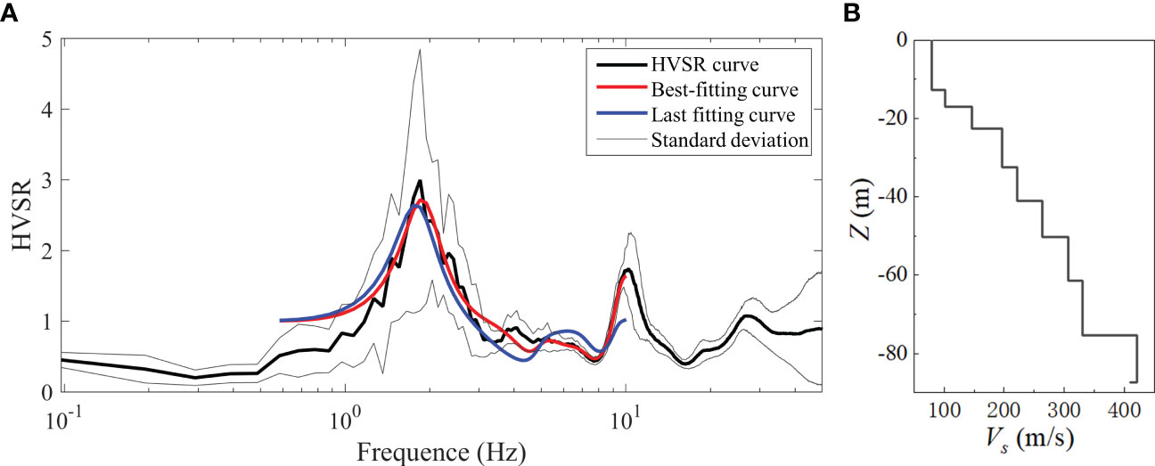
Figure 3 Example of inversion of marine ambient noise recording. (A) Best-fit model. (B) The structure of shear wave velocity corresponding to the best-fit model.

To evaluate the accuracy of the inversion, we used two concepts: global misfit and local misfit. Local misfit refers to the normalized misfit between the simulated and experimental curve at each station. For the global misfit, we introduced the objective function (Bignardi et al., 2018):

$$E(m)=aM(m)+bS(m)+{\displaystyle \sum _{j=1}^5{\alpha }_j{R}_j(m)}$$

Where M(m) represents the misfit between the simulated and experimental curves; S(m) represents the fitting degree of the simulated and experimental curves at the peaks; and R_j(m) represents the regularization term. The constants a and b in above Equation are used to balance the relative weight of the M(m) and S(m) terms. Based on the objective function, we define the global misfit as aM(m) + bS(m).

Figure 4A shows the global misfit of the inversion results. As can be seen from the figure that the global misfit between the inversion results and experimental data is 0.1, and the fitting degree at the peak of the experimental curve and simulated curve is around 0.9. The normalized misfit between the experimental data and simulated data at each station is shown in Figure 4B, and it can be seen that there are 52 stations with a local misfit of less than 0.1; 6 stations with a local misfit between 0.1 to 0.2; and only 6 stations have a local misfit exceeding 0.2.

FIGURE 4

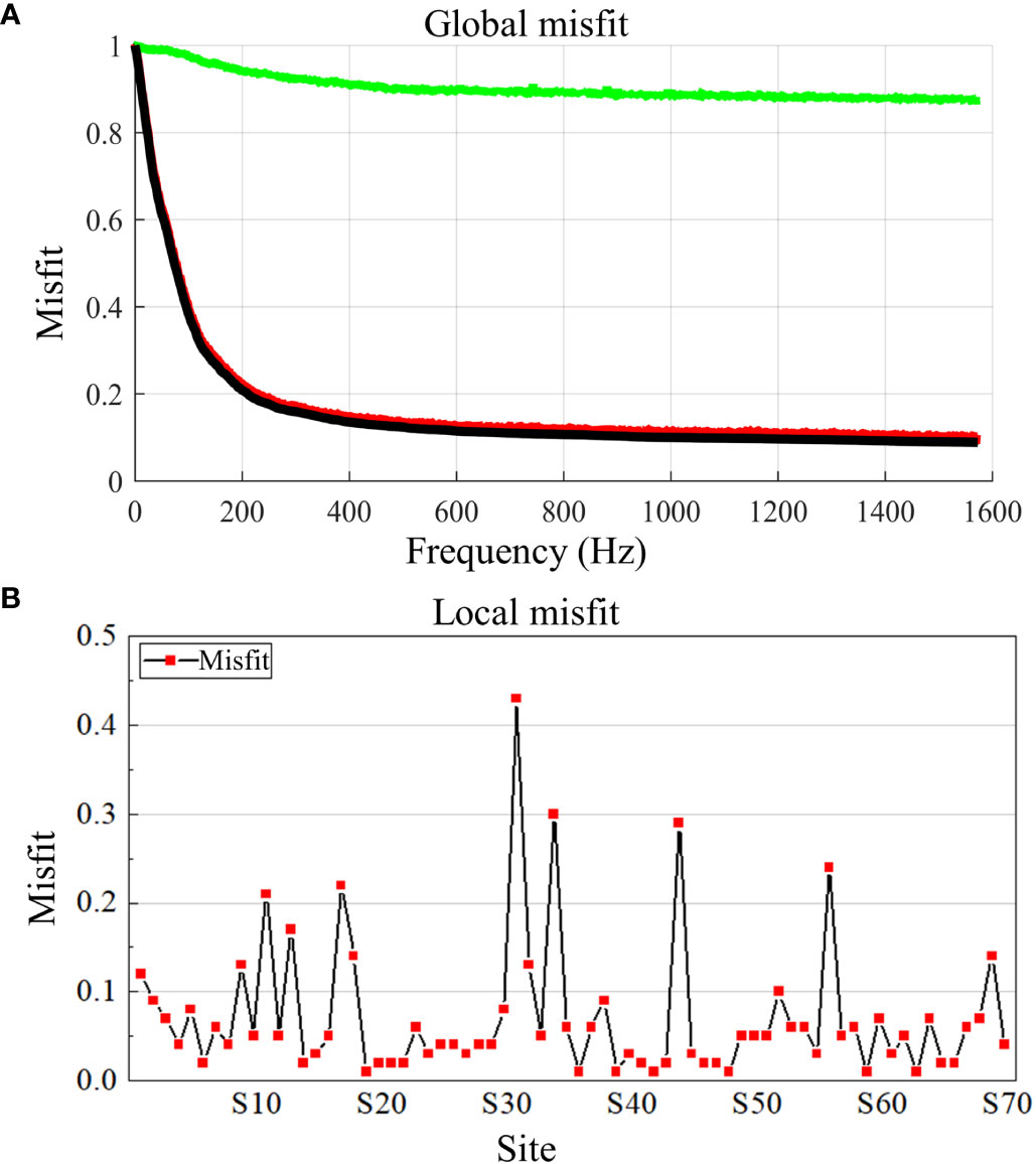
Figure 4 Value of the normalized misfit. (A) Global misfit, where the black curve represents the misfit of the inversion results (the aM(m)+bS(m) in Equation); the red curve is the misfit of the experimental and simulated curves (the aM(m) in Equation); and the green curve is the fitting degree at the peak of the experimental and simulated curves (the bS(m) in Equation). (B) Normalized misfit for each station at the end of the inversion.

4 Results and discussion

4.1 Characteristics of ocean ambient noise

Ocean ambient noise is a persistent acoustic field in the ocean, and different sources produce noise of different frequencies (Bonnefoy-Claudet et al., 2006). The movement of the Earth’s crust is the primary source of ultra-low frequency noise in the ocean, with quasi-periodicity of 1-7 Hz; nonlinear interaction of back-propagating sea surface waves produces random noise with frequencies between 5-10 Hz; sound waves emitted by atmospheric sources (such as lightning) can couple into the underwater sound field, with frequencies also below 10 Hz; ship navigation produces sound waves with frequencies ranging from 5-500 Hz; and deep-sea currents, internal solitary waves, and turbulence caused by fragmentation create a wider frequency range. In the coastal and nearshore noise fields, waves, as the primary source of noise, waves striking along the coasts are the main source of low-frequency noise with a range of 0.5-1.2 Hz (Gutenberg, 1958), and the strong interaction between waves with the seabed can generate noise up to 10 Hz (Olofsson, 2010). In this paper, we concern the ambient noise with frequency below 10 Hz.

We conducted ocean ambient noise recordings using the single-station array and the centerless circular array with a radius of 1 m on the tidal flats in the Yellow River Delta. Figure 5 shows the Fourier spectrum of ocean ambient noise recorded by six stations in the centerless circular array. There is a certain energy of ambient noise in each station from low to high frequencies. The Fourier spectrum shows good amplitude consistency in the low-frequency band (1.9-7.7 Hz) and differentiation in the high-frequency band. Thus, it could be considered that the ocean ambient noise propagates in all directions with almost the same energy in each direction within this band. According to the analysis of the characteristics, the ocean ambient noise recorded on the tidal flats in the Yellow River Delta shows a good consistency in the low-frequency band and relative dispersion in the high-frequency band. We analyze that the factors such as waves, tides, and wind are the main sources of noise on the tidal flats, so the recorded noise mainly presents low-frequency and long-wavelength characteristics, and of course, it also contains some high-frequency and short-wavelength noise generated by the navigation. Compared with land ambient noise, ocean ambient noise dominates in the low-frequency band, which can be used to obtain deeper seabed soil information.

FIGURE 5

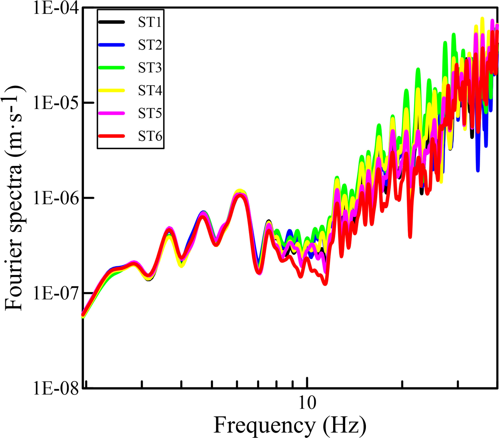
Figure 5 Fourier spectrum of ambient noise recorded by six stations in a centerless circular array.

4.2 Inversion results of shear wave velocity

After obtaining the inversion results, the distribution of shear wave velocity within the depth range of 0-100 m was statistically analyzed. The confidence intervals of the shear wave velocity at the confidence levels of 95% and 75% were also calculated, as shown in Table 2. The accuracy and applicability of the inverted shear wave velocity were tested by comparing them with the field measurements (Liu et al., 2015).

TABLE 2

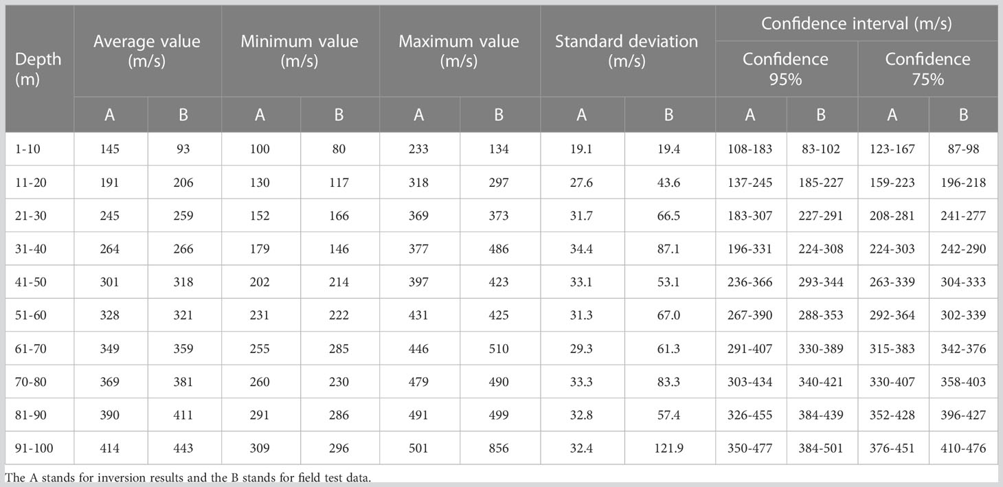
Table 2 Distribution of shear wave velocity obtained by HVSR curves inversion and measured field data from Liu et al. (2015).

From Table 2, it can be found that the average, minimum and maximum values of shear wave velocity obtained by inversion are basically consistent with the field measurements at depths of 10-90 m depth. However, the ranges of shear wave velocities obtained from the inversion are underestimated in the depth of 0-10 m. Among them, the shear wave velocity obtained from the inversion respectively are 83-102 m/s and 87-98 m/s at 90% and 75% confidence intervals, which deviate from the field results of 108-183 m/s and 123-167 m/s. The inversion results are lower compared with the measured results, -which is speculated to be related to the groundwater table. The field measurements of shear wave velocity were carried out at locations far from the sea, while the study area is located in the coastal zone with extremely shallow groundwater table and high soil moisture content, resulting in a lower shear wave velocity. Within the range of 10-90 m, the distribution of the inverted shear wave velocity in the stratum satisfies the results of the field measurements at the 95% and 75% confidence intervals. Nevertheless, in the depth range below 30 m, the maximum value of the shear wave velocity and the lower limit of the 95% confidence interval are both higher than the measured data. Moreover, there exist an abnormally high value for the inverted shear wave velocity at the bottom layer.

Liu et al. (2007) conducted shear wave velocity tests on the northern coastal zone in the Yellow River Delta and obtained measured shear wave velocities of 91-137 m/s within the depth range of 0-10 m (Table 3). Yang et al. (2022) carried out field measurements using the single-hole method on tidal flats in the Yellow River Delta, and the measured shear wave velocities were mainly distributed in a range of 100-250 m/s within the depth range of 0-20 m. The inverted results are in good agreement with the field measurements, which further proves the accuracy of the inversion shear wave velocities.

TABLE 3

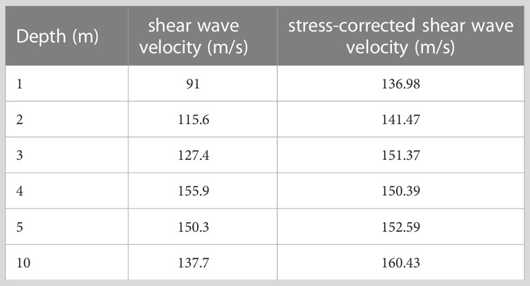
Table 3 Field measured shear wave velocity and calculated critical shear wave velocity in the Yellow River Delta (modified from Liu et al., 2007).

4.3 Shear wave velocity threshold

Andrus and Stokoe (Andrus and Stokoe, 1999; Andrus and Stokoe, 2000; Andrus et al., 2004) proposed a simplified method for soil liquefaction assessment using shear wave velocity (V_s) and stress-corrected shear wave velocity (V_s1) based on a large amount of investigations of earthquake liquefaction occurring in fine-grained soils, such as fine sand, gravel, and silty clay. For Holocene unconsolidated fine-grained soil, Youd and Idriss (2001) established the relationship between V_s and cyclic stress ratio (CSR) for liquefaction and non-liquefaction areas according to a probabilistic statistical method and proposed the upper limit of V_s (180 m/s) as a threshold for liquefaction assessment in engineering practice (Yulianur et al., 2020). However, statistical analysis of the relationship between stress-corrected shear wave velocity and CSR revealed certain limitations of this threshold. To illustrate this viewpoint, we collected the investigation data from over 50 different locations. The liquefaction areas were determined by the observation of liquefaction phenomena and in-situ tests (SPT and CPT). The relationship between the cyclic stress ratio (CSR) and shear wave velocity or stress-corrected shear wave velocity is established based on probabilistic statistics of the distribution of shear wave velocity.

Figure 6A shows the relationship between CSR and the measured average V_s in liquefaction and non-liquefaction fields, and Figure 6B presents the relationship between CSR and V_s1. The measured V_s of soils in liquefaction area ranged from 79 to 210 m/s, generally lower than 180 m/s, with only four data exceeding this threshold for an error of about 4%. Differently, the distribution of V_s1 ranged from 104 to 271 m/s, with 15% of the data exceeding 180 m/s. As a result, it may be risky to use the shear wave velocity of 180 m/s as the threshold for soil liquefaction assessment in practical engineering applications. The confidence interval of V_s1 in 95% confidence is 149.10-160.47 m/s, with 95% of the data below 200 m/s. Accordingly, it is considered that 200 m/s as the threshold for liquefaction assessment of fine-grained soils will be of practical application.

FIGURE 6

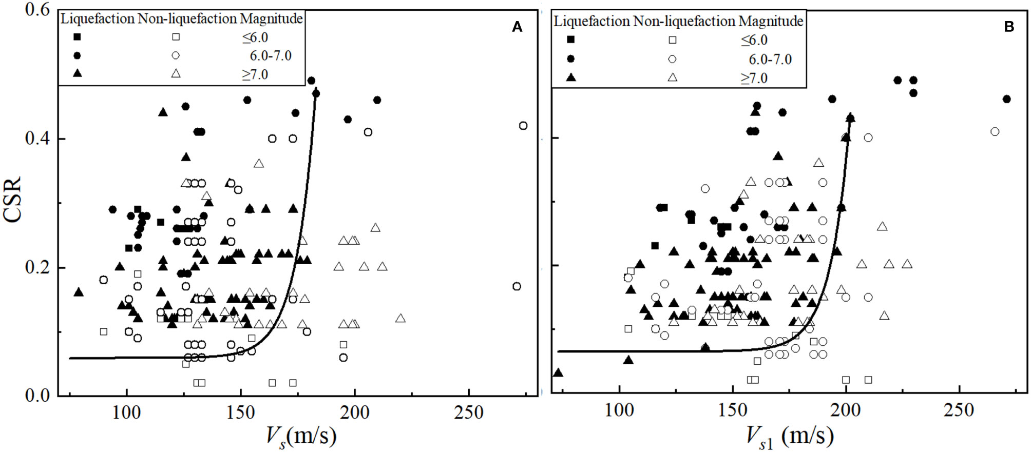
Figure 6 V_s -based liquefaction and non-liquefaction for Holocene unconsolidated fine-grained soils. (A) The relationship between the measured V_s and cyclic stress ratio (CSR). (B) The relationship between V_s1 and CSR. In the figures, the square, circle and triangle represent respectively shear wave velocities of soils with earthquake magnitudes ≤6.0, 6.0-7.0, ≥7.0; the solid and hollow figures correspond to shear wave velocities liquefaction and non-liquefaction areas respectively.

4.4 Soil liquefaction assessment

According to the statistics of the field investigation data for soil liquefaction, wave-induced soil liquefaction generally occurs in shallow surface seabed within a few meters (Hirst and Richards, 1977; Sassa et al., 2006), and depth of the seismic liquefaction may occur up to 20 m below the surface in the gravel, and the depth in silt and silty sand is commonly less than 20 m (Holzer et al., 1999; Bray et al., 2004). Liu et al. (2005) considered that the silt soils in the Yellow River Delta have liquefaction potential under dynamic loads based on the pore-pressure model. As shown in Tables 2, the inverted shear wave velocity is in general agreement with the field measured results within 30 m depth. Consequently, it can be used to evaluate problems such as seabed soil liquefaction.

Figure 7 shows the shear wave velocity structures of three areas on the coastal zone. The red dashed line and solid line represent the dividing lines of shear wave velocity of 180 m/s and 200 m/s, respectively. It can be seen that the vertical distribution of shear wave velocity corresponds roughly to the boundaries of soil indicated by the borehole Yang et al. (2022). Moreover, the shear wave velocity of the soil within a depth of 10 m is generally less than 200 m/s, indicating that the fine-grained soil at this depth has a certain potential for liquefaction. Liu et al. (2007) calculated the critical shear wave velocity within the range of 0-10 m based on the empirical relationship between shear wave velocity and the number of blows of standard penetration, which is found to be from 136 to 160 m/s (Table 3). The inverted shear wave velocity within the depth range of 0-10 m is determined to be between 80-133.87 m/s, which is lower than the critical shear wave velocity for each layer. Therefore, it is determined that the soil within the range of 0-10 m on the tidal flat was judged to be liquefiable. The results of the soil liquefaction assessment based on the shear wave velocity threshold and the critical shear wave velocity were consistent within the depth range of 0-10 m. Meanwhile, it can be observed that there were multiple low-velocity anomalies in the vertical shear wave velocity structure of the strata, and there were significant differences in the shear wave velocity of the soil at the same depth range in the lateral direction. As shown in Figure 7, from the coastal plain to the tidal flat in front of the embankment, the shear wave velocity of the soil follows the trend of gradually decreasing from land to sea. According to geological data in the region, the high-concentration sediment continuously accumulates during the transportation process of the river due to oscillation and diversion of the Yellow River estuary, sea level changes, and the combined effects of waves, tides, and storm surges. The fluvial deposits and coastal deposits in different periods have been superimposed and deposited, forming a sedimentary structure that appears as a finger-like interlocking in the horizontal direction, and the gradually advancing from land to sea in the vertical direction. In different depth ranges, there are marine deposits with high water content and high saturation, as well as soft soil layers with high water content, high porosity ratio, and low shear strength, which are unevenly distributed in the tidal flat. This results in the common presence of low-velocity abnormal segments in the shear wave velocity structure.

FIGURE 7

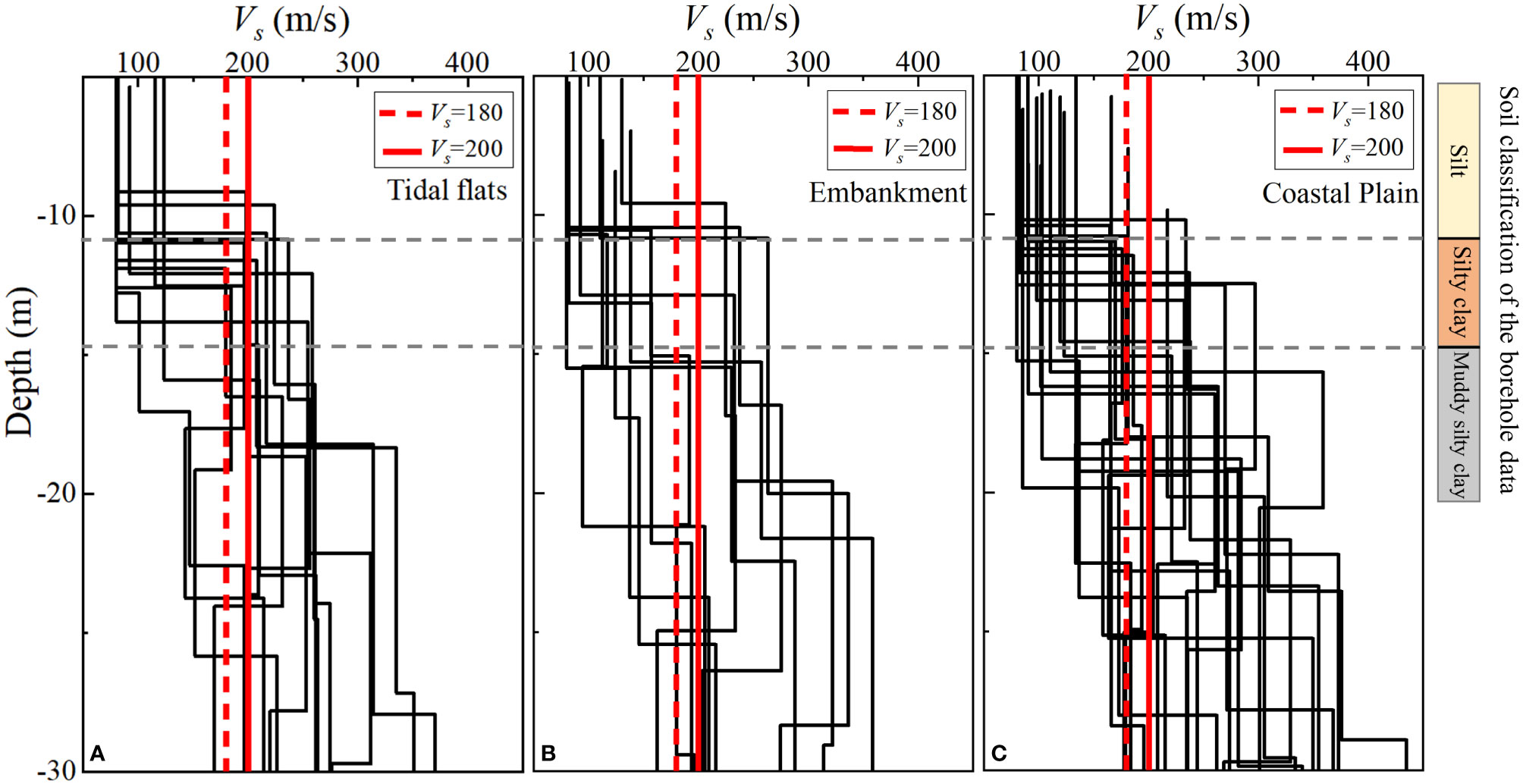
Figure 7 1-D shear wave velocity structure within 30 m depth at each station. The Yellow River delta is divided into three study areas, namely (A) the tidal flats area in front of the embankment, (B) the embankment area, and (C) the coastal plain area. The bar in the figure represent the soil layer classification, and the borehole data is cited from Yang et al. (2022).

A measuring line was set up along the east-west direction on the tidal flat in front of the embankment in the Yellow River Delta. Figure 8 shows the inversion results of seven observation stations on the tidal flat. Figure 8A shows the shear wave velocity profile within a depth range of 30 m. For comparison, we first converted the frequency to “pseudo-depth” using the quarter-wavelength formula (h=V_s/4f) to obtain the HVSR curve with depth, then, we plotted the HVSR profiles in Figure 8B with interpolation method based on all curves. The figure shows that the shear wave velocity of the geological layer exhibits a layered distribution, which is consistent with the sedimentary characteristics of the region. Geological layers with a shear wave velocity less than 200 m/s are distributed within a depth range of 10 m, and some stations can reach 20 m. The distribution of the HVSR shows a negative correlation with the magnitude of the shear wave velocity (Figure 8B). The level of the horizontal and vertical spectral ratio of ambient noise reflects the amplification effect of the soil on seismic motion. The looser the soil, the more significant the amplification effect of the seismic wave amplitude is, while the noise spectral ratio is larger. At the same time, soft soil has a lower degree of compaction and a lower shear wave velocity. It can be understood that the shear wave velocity of the surface soil of the tidal flats is low and its engineering properties are poor. Soft surface soil will amplify the amplitude and energy of seismic waves. If seismic waves in a certain frequency band coincide with the resonance frequency of the overlying soil, the resonance effect will be induced, which will cause unpredictable damage to the overlying buildings.

FIGURE 8

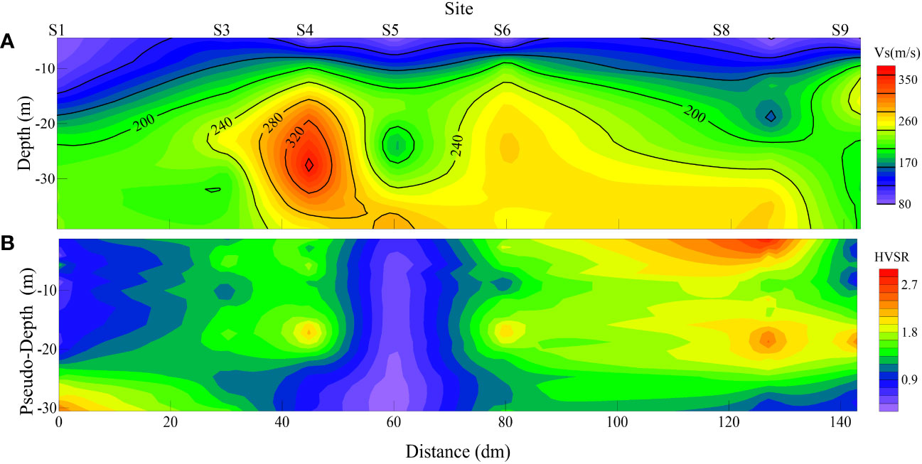
Figure 8 Inversion results along the east-west lateral line of 7 observation stations on the tidal flat in the Yellow River Delta. (A) 2-D Shear wave velocity profile of the tidal flat. (B) For comparison, the HVSR profile is formed by the HVSR curves, and the frequency axis is converted to “pseudo-depth” by the assumption that V_s=350 m/s for soft layers.

5 Conclusion

The purpose of this paper is to obtain the shear wave velocity of seabed soils by inversion of ocean ambient noise for rapid assessment of seabed soil liquefaction. In-situ noise recording and analysis were performed in the northern coast of the Yellow River Delta using the HVSR method to obtain the shear wave velocity of the seabed soil. Based on statistical analysis of liquefaction investigation data, a shear wave velocity threshold was proposed for assessing the liquefaction potential, and the location of liquefiable soil was identified in the light of 1-D shear wave velocity structure and 2-D shear wave velocity profile. In summary, the following results were obtained:

1. Ocean ambient noise has the characteristics of low-frequency, long-wavelength, and wide bandwidth. Therefore, in-situ observations of ocean ambient noise can not only obtain the physical and mechanical properties of the seabed soil in a deeper range depending on the propagation characteristics of noise in the seabed sediment, but also monitor the deformation and stability of the seabed soil, provide the necessary support for the design and construction of marine engineering, and are of great significance for risk assessment and the early warning of marine geology disasters.

2. Shear wave velocities of seabed soils were obtained by inversing the HVSR dataset of oceanic ambient noise. The stratigraphic distribution of the shear wave velocity obtained by inversion is broadly consistent with existing research results, which indicates that the results have a certain degree of accuracy and that the method for inverting ocean ambient noise is quite feasible.

3. The application of a shear wave velocity threshold of 200 m/s in assessing the liquefaction potential of fine-grained soils in the Yellow River Delta yielded consistent results with traditional methods. The assessment showed the liquefaction potential of soil in depths of 0-10 m, and indicated that this threshold is reasonable for liquefaction assessment of seabed soil in the Yellow River Delta. Accordingly, the stability problems of the soil in the tidal flat area should be taken into sufficient consideration during engineering construction. It is necessary to adopt measures such as replacement methods and dynamic consolidation for foundation treatment to ensure the safety of engineering construction and use.

4. The HVSR-based ocean ambient noise prospecting method has the advantages of being convenient, economical, environment-independent, and deeper detection depth. It can provide services for disaster prevention and mitigation of marine engineering construction, and has good practical application. In addition, in the actual application process, combining this method with other geotechnical tests (such as drilling, in-situ tests, or laboratory tests, etc.) can more accurately determine the engineering characteristics of soil, and further classify the liquefaction hazard of soil, which is crucial for coastal protection and marine engineering construction.

Data availability statement

The raw data supporting the conclusions of this article will be made available by the authors, without undue reservation.

Author contributions

Conceptualization & methodology, YL, QM and SW. Formal analysis, YL and WW. Data curation, YL and YC. Writing—original draft preparation, YL. Writing—review & editing, YL and QM. Visualization, YC and SW. Project administration, YL and WW. Funding acquisition, QM. All authors contributed to the article and approved the submitted version.

Funding

The study is supported by the National Natural Science Foundation of China (Nos. 42272327), and the Social and livelihood project of Shandong Province (2021, 202131001).

Acknowledgments

The authors would like to thank Zhiyuan Chen who participated in recording the ambient noise in the field and Yupeng Ren who participated in revising the manuscript.

Conflict of interest

The authors declare that the research was conducted in the absence of any commercial or financial relationships that could be construed as a potential conflict of interest.

Publisher’s note

All claims expressed in this article are solely those of the authors and do not necessarily represent those of their affiliated organizations, or those of the publisher, the editors and the reviewers. Any product that may be evaluated in this article, or claim that may be made by its manufacturer, is not guaranteed or endorsed by the publisher.

References

Aki K. (1957). Space and time spectra of stationary stochastic waves, with special reference to microtremors. Bull. Earthq. Eng. 35, 414–456.

Google Scholar

Amini F., Qi G. Z. (2000). Liquefaction testing of stratified silty sands. J. Geotech. Geoenviron. Eng. 126, 208–217. doi: 10.1061/(ASCE)1090-0241(2000)126:3(208

CrossRef Full Text | Google Scholar

Andrus R. D., Stokoe K. H. (1999). Liquefaction resistance based on shear wave velocity. Proceed. NCEER Workshop Eval. Liquefact. Resist. Soils. 22, 89–128. doi: 10.1186/s40703-020-00132-1

CrossRef Full Text | Google Scholar

Andrus R. D., Stokoe K. H. (2000). Liquefaction resistance of soils from shear-wave velocity. J. Geotech. Geoenviron. Eng. 126, 1015–1025. doi: 10.1061/(ASCE)1090-0241(2000)126:11(1015

CrossRef Full Text | Google Scholar

Andrus R. D., Stokoe K. H., Hsein Juang C. (2004). Guide for shear-wave-based liquefaction potential evaluation. Earthq. Spectra 20, 285–308. doi: 10.1193/1.1715106

CrossRef Full Text | Google Scholar

Bachrach R., Nur A., Agnon A. (2001). Liquefaction and dynamic poroelasticity in soft sediments. J. Geophys. Res. 106, 13515–13526. doi: 10.1029/2000JB900474

CrossRef Full Text | Google Scholar

Bignardi S., Yezzi A. J., Fiussello S., Comelli A. (2018). OpenHVSR - processing toolkit: enhanced HVSR processing of distributed microtremor measurements and spatial variation of their informative content. Comput. Geosci. 120, 10–20. doi: 10.1016/j.cageo.2018.07.006

CrossRef Full Text | Google Scholar

Bonnefoy-Claudet S., Cotton F., Bard P.-Y. (2006). The nature of noise wavefield and its applications for site effects studies: a literature review. Earth-Sci. Rev. 79, 205–227. doi: 10.1016/j.earscirev.2006.07.004

CrossRef Full Text | Google Scholar

Boore D. M. (2003). Simulation of ground motion using the stochastic method. Pure Appl. Geophys. 160, 635–676. doi: 10.1007/PL00012553

CrossRef Full Text | Google Scholar

Boumpoulis V., Depountis N., Pelekis P., Sabatakakis N. (2021). SPT and CPT application for liquefaction evaluation in Greece. Arab. J. Geosci. 14, 1631. doi: 10.1007/s12517-021-08103-1

CrossRef Full Text | Google Scholar

Bray J. D., Sancio R. B., Durgunoglu T., Onalp A., Youd T. L., Stewart J. P., et al. (2004). Subsurface characterization at ground failure sites in adapazari, Turkey. J. Geotech. Geoenviron. Eng. 130, 673–685. doi: 10.1061/(ASCE)1090-0241(2004)130:7(673)

CrossRef Full Text | Google Scholar

Bromirski P. D., Duennebier F. K., Stephen R. A. (2005). Mid-ocean microseisms. Geochem. Geophys. Geosyst. 6 (4), Q04009. doi: 10.1029/2004GC000768

CrossRef Full Text | Google Scholar

Dassanayake S. M., Mousa A. A., Ilankoon S., Fowmes G. J. (2022). Internal instability in soils: a critical review of the fundamentals and ramifications. Transp. Res. Rec. 2676, 1–26. doi: 10.1177/03611981211056908

CrossRef Full Text | Google Scholar

Dobry R., Abdoun T. (2017). Recent findings on liquefaction triggering in clean and silty sands during earthquakes. J. Geotech. Geoenviron. Eng. 143, 04017077. doi: 10.1061/(ASCE)GT.1943-5606.0001778

CrossRef Full Text | Google Scholar

Edwards B., Poggi V., Fah D. (2011). A predictive equation for the vertical-to-horizontal ratio of ground motion at rock sites based on shear-wave velocity profiles from Japan and Switzerland. Bull. Seismol. Soc Amer. 101, 2998–3019. doi: 10.1785/0120110023

CrossRef Full Text | Google Scholar

Fergany E., Omar K. (2017). Liquefaction potential of Nile delta, Egypt. NRIAG J. Astron. Geophys. 6, 60–67. doi: 10.1016/j.nrjag.2017.01.004

CrossRef Full Text | Google Scholar

Field E. H., Hough S. E., Jacob K. H. (1990). Using microtremors to assess potential earthquake site response: a case study in flushing meadows, new York city. Bull. Seismol. Soc Amer. 80, 1456–1480. doi: 10.1785/BSSA08006A1456

CrossRef Full Text | Google Scholar

Field E., Jacob K. (1993). The theoretical response of sedimentary layers to ambient seismic noise. Geophys. Res. Lett. 20, 2925–2928. doi: 10.1029/93GL03054

CrossRef Full Text | Google Scholar

Geyin M., Maurer B. W. (2021). Evaluation of a cone penetration test thin-layer correction procedure in the context of global liquefaction model performance. Eng. Geol. 291, 106221. doi: 10.1016/j.enggeo.2021.106221

CrossRef Full Text | Google Scholar

Gorgas T. J., Wilkens R. H., Fu S. S., Frazer L. N., Richardson M. D., Briggs K. B., et al. (2002). In situ acoustic and laboratory ultrasonic sound speed and attenuation measured in heterogeneous soft seabed sediments: eel river shelf, California. Mar. Geol. 182, 103–119. doi: 10.1016/S0025-3227(01)00230-4

CrossRef Full Text | Google Scholar

Gutenberg B. (1958). Microseisms. Adv. Geophys. 5, 53–92. doi: 10.1016/S0065-2687(08)60075-8

CrossRef Full Text | Google Scholar

Hardin B. O., Drnevich V. P. (1972). Shear modulus and damping in soils: design equations and curves. J. Soil Mech. Found. Eng. 98, 667–692. doi: 10.1061/JSFEAQ.0001760

CrossRef Full Text | Google Scholar

Hasselmann K. (1963). A statistical analysis of the generation of microseisms. Rev. Geophys. 1, 177–210. doi: 10.1029/RG001i002p00177

CrossRef Full Text | Google Scholar

Hirst T. J., Richards A. F. (1977). In situ pore-pressure measurement in Mississippi delta front sediments. Mar. Geotech. 2, 191–204. doi: 10.1080/10641197709379779

CrossRef Full Text | Google Scholar

Holzer T. L., Bennett M. J., Ponti D. J., Tinsley J. C. (1999). Liquefaction and soil failure during 1994 northridge earthquake. J. Geotech. Geoenviron. Eng. 125, 438–452. doi: 10.1061/(ASCE)1090-0241(1999)125:6(438

CrossRef Full Text | Google Scholar

Hou Z., Chen Z., Wang J., Zheng X., Yan W., Tian Y., et al. (2018). Acoustic characteristics of seafloor sediments in the abyssal areas of the south China Sea. Ocean Eng. 156, 93–100. doi: 10.1016/j.oceaneng.2018.03.013

CrossRef Full Text | Google Scholar

Jeng D. S. (2001). Mechanism of the wave-induced seabed instability in the vicinity of a breakwater: a review. Ocean Eng. 28, 537–570. doi: 10.1016/S0029-8018(00)00013-5

CrossRef Full Text | Google Scholar

Jia Y., Zheng J., Yue Z., Liu X., Shan H. (2014). Tidal flat erosion of the huanghe river delta due to local changes in hydrodynamic conditions. Acta Oceanol. Sin. 33, 116–124. doi: 10.1007/s13131-014-0501-y

CrossRef Full Text | Google Scholar

Joyner W. B., Warrick R. E., Fumal T. E. (1981). The effect of quaternary alluvium on strong ground motion in the coyote lake, California, earthquake of 1979. Bull. Seismol. Soc Amer. 71, 1333–1349. doi: 10.1785/BSSA0710041333

CrossRef Full Text | Google Scholar

Kawase H., Sanchez-Sesma F., Matsushima S. (2011). The optimal use of horizontal-to-vertical spectral ratios of earthquake motions for velocity inversions based on diffuse-field theory for plane waves. Bull. Seismol. Soc Amer. 101, 2001–2014. doi: 10.1785/0120100263

CrossRef Full Text | Google Scholar

Kumar S. S., Murali Krishna A., Dey A. (2020). Assessment of dynamic response of cohesionless soil using strain-controlled and stress-controlled cyclic triaxial tests. Geotech. Geol. Eng. 38, 1431–1450. doi: 10.1007/s10706-019-01100-y

CrossRef Full Text | Google Scholar

Lin A., Wotherspoon L., Bradley B., Motha J. (2021). Evaluation and modification of geospatial liquefaction models using land damage observational data from the 2010–2011 Canterbury earthquake sequence. Eng. Geol. 287, 106099. doi: 10.1016/j.enggeo.2021.106099

CrossRef Full Text | Google Scholar

Liu X., Jia Y., Zheng J., Hou W., Zhang L., Zhang L.-P., et al. (2013). Experimental evidence of wave-induced inhomogeneity in the strength of silty seabed sediments: yellow river delta, China. Ocean Eng. 59, 120–128. doi: 10.1016/j.oceaneng.2012.12.003

CrossRef Full Text | Google Scholar

Liu X., Liu H., Jia Y. (2007). Investigation on prediction methods and characteristics of earthquake-induced liquefaction of silty soil in the yellow river delta. Chin. J. Rock Mech. Eng. (in Chinese). 26, 2981–2987. doi: 10.3321/j.issn:1000-6915.2007.z1.060

CrossRef Full Text | Google Scholar

Liu F., Liu L., Liu J. (2015). Characteristic analysis of shear wave velocity of the yellow river delta. China Eng. Consult. (in Chinese) 10, 90–93. doi: 10.3969/j.issn.1006-9607.2015.10.017

CrossRef Full Text | Google Scholar

Liu H., Wang X., Jia Y., Qiao S., Zhang H. (2005). Experimental study on liquefaction properties and pore-water pressure model of saturated silt in yellow river delta. Rock Soil Mech. (in Chinese). 26, 83–87. doi: 10.16285/j.rsm.2005.s2.046

CrossRef Full Text | Google Scholar

Liu X., Wang Y., Zhang H., Guo X. (2023). Susceptibility of typical marine geological disasters: an overview. Geoenviron. Disasters 10, 10. doi: 10.1186/s40677-023-00237-6

CrossRef Full Text | Google Scholar

Meng Q., Li Y., Wang W., Chen Y., Wang S. (2023). A case study assessing the liquefaction hazards of silt sediments based on the horizontal-to-vertical spectral ratio method. J. Mar. Sci. Eng. 11, 104. doi: 10.3390/jmse11010104

CrossRef Full Text | Google Scholar

Meng Q., Liu S., Jia Y., Xiao Z., Wang X. (2018). Analysis on acoustic velocity characteristics of sediments in the northern slope of the south China Sea. Bull. Eng. Geol. Environ. 77, 923–930. doi: 10.1007/s10064-017-1070-z

CrossRef Full Text | Google Scholar

Nakamura Y. (1989). A method for dynamic characteristics estimation of subsurface using microtremor on the ground surface. Q. Rep. RTRI. 30 (1), 25–33.

Google Scholar

Nakamura Y. (2000). Clear identification of fundamental idea of nakamura’s technique and its applications. Proc. XII World Conf. Earthquake Eng. 3, 2656.

Google Scholar

Nakamura Y. (2008). On the H/V spectrum. In The 14th Word Conference on Earthquake Engineering, Beijing, China. 12–17.

Google Scholar

Nakamura Y. (2009). “Basic structure of QTS (HVSR) and examples of applications,” in Increasing seismic safety by combining engineering technologies and seismological data NATO science for peace and security series c: environmental security. Eds. Mucciarelli M., Herak M., Cassidy J. (Dordrecht: Springer Netherlands), 33–51. doi: 10.1007/978-1-4020-9196-4_4

CrossRef Full Text | Google Scholar

Nakamura Y. (2019). What is the Nakamura method? Seismol. Res. Lett. 90, 1437–1443. doi: 10.1785/0220180376

CrossRef Full Text | Google Scholar

Olofsson B. (2010). Marine ambient seismic noise in the frequency range 1-10 Hz. Lead. Edge 29, 418–435. doi: 10.1190/1.3378306

CrossRef Full Text | Google Scholar

Qin L., Ben-Zion Y., Bonilla L. F., Steidl J. H. (2020). Imaging and monitoring temporal changes of shallow seismic velocities at the garner valley near anza, California, following the M7.2 2010 El mayor-cucapah earthquake. J. Geophys. Res. Solid Earth 125, e2019JB018070. doi: 10.1029/2019JB018070

CrossRef Full Text | Google Scholar

Ren Y., Xu G., Xu X., Zhao T., Wang X. (2020). The initial wave induced failure of silty seabed: liquefaction or shear failure. Ocean Eng. 200, 106990. doi: 10.1016/j.oceaneng.2020.106990

CrossRef Full Text | Google Scholar

Sassa S., Takayama T., Mizutani M., Tsujio D. (2006). Field observations of the build-up and dissipation of residual pore pressures in seabed sands under the passage of storm waves. J. Coast. Res. 39, 410–414. doi: 10.1007/s00367-020-00680-6

CrossRef Full Text | Google Scholar

Seed H. B., Idriss I. M., Arango I. (1983). Evaluation of liquefaction potential using field performance data. J. Geotech. Eng. 109, 458–482. doi: 10.1061/(ASCE)0733-9410(1983)109:3(458

CrossRef Full Text | Google Scholar

Sumer B. (2014). Advances in seabed liquefaction and its implications for marine structures. Geotech. Eng. 45, 1–14. doi: 10.1007/s40722-014-0005-z

CrossRef Full Text | Google Scholar

Sumer B. M., Fredsøe J., Christensen S., Lind M. T. (1999). Sinking/floatation of pipelines and other objects in liquefied soil under waves. Coast. Eng. 38, 53–90. doi: 10.1016/S0378-3839(99)00024-1

CrossRef Full Text | Google Scholar

Tokimatsu K., Uchida A. (1990). Correlation between liquefaction resistance and shear wave velocity. Soils Found. 30, 33–42. doi: 10.3208/sandf1972.30.2_33

CrossRef Full Text | Google Scholar

Toksoz M. N. (1964). Microseisms and an attempted application to exploration. Geophysics 29, 154–177. doi: 10.1190/1.1439344

CrossRef Full Text | Google Scholar

Tsai N. C., Housner G. W. (1970). Calculation of surface motions of a layered half-space. Bull. Seismol. Soc Amer. 60, 1625–1651. doi: 10.1785/BSSA0600051625

CrossRef Full Text | Google Scholar

Wang Y., Cao T., Gao Y., Shao J. (2022). Experimental study on liquefaction characteristics of saturated yellow river silt under cycles loading. Soil Dyn. Earthq. Eng. 163, 107457. doi: 10.1016/j.soildyn.2022.107457

CrossRef Full Text | Google Scholar

Xu X., Ling D., Cheng Y., Chen Y. (2015). Correlation between liquefaction resistance and shear wave velocity of granular soils: a micromechanical perspective. Géotechnique 65, 337–348. doi: 10.1680/geot.SIP.15.P.022

CrossRef Full Text | Google Scholar

Yang Z., Cui Y., Guo L., Liu X., Jia C., Shi W., et al. (2022). Semi-empirical correlation of shear wave velocity prediction in the yellow river delta based on CPT. Mar. Geores. Geotechnol. 40, 487–499. doi: 10.1080/1064119X.2021.1913458

CrossRef Full Text | Google Scholar

Ye B., Hu H., Bao X., Lu P. (2018). Reliquefaction behavior of sand and its mesoscopic mechanism. Soil Dyn. Earthq. Eng. 114, 12–21. doi: 10.1016/j.soildyn.2018.06.024

CrossRef Full Text | Google Scholar

Ye J., Jeng D., Chan A., Wang R., Zhu Q. (2016). 3D integrated numerical model for fluid-structures-seabed interaction (FSSI): elastic dense seabed foundation. Ocean Eng. 115, 107–122. doi: 10.1016/j.oceaneng.2016.01.003

CrossRef Full Text | Google Scholar

Youd T. L., Idriss I. M. (2001). Liquefaction resistance of soils: summary report from the 1996 NCEER and 1998 NCEER/NSF workshops on evaluation of liquefaction resistance of soils. J. Geotech. Geoenviron. Eng. 127, 297–313. doi: 10.1061/(ASCE)1090-0241(2001)127:4(297

CrossRef Full Text | Google Scholar

Yulianur A., Saidi T., Setiawan B., Sugianto S., Rusdi M. (2020). Microtremor measurement at liquefaction-induced ground deformation area. J. Eng. Sci. Technol. 15, 2871–2889. Available at: https://jestec.taylors.edu.my/Vol%2015%20issue%205%20October%202020/15_5_2.pdf

Google Scholar

Zhang H., Lu Y., Liu X., Li X., Wang Z., Ji C., et al. (2023). Morphology and origin of liquefaction-related sediment failures on the yellow river subaqueous delta. Mar. Pet. Geol. 153, 106262. doi: 10.1016/j.marpetgeo.2023.106262

CrossRef Full Text | Google Scholar

Zhang Q., Zhou X., Wang J., Guo J. (2017). Wave-induced seabed response around an offshore pile foundation platform. Ocean Eng. 130, 567–582. doi: 10.1016/j.oceaneng.2016.12.016

CrossRef Full Text | Google Scholar

Zhao H., Jeng D. (2015). Numerical study of wave-induced soil response in a sloping seabed in the vicinity of a breakwater. Appl. Ocean Res. 51, 204–221. doi: 10.1016/j.apor.2015.04.008

CrossRef Full Text | Google Scholar

Zhao H., Jeng D., Liao C., Zhang J., Guo Z., Chen W. (2018). Numerical modelling of liquefaction in loose sand deposits subjected to ocean waves. Appl. Ocean Res. 73, 27–41. doi: 10.1016/j.apor.2018.01.011

CrossRef Full Text | Google Scholar

Zhao G., Te Q., Xue C., Ma Y., Ye S. (2013). Surface sediments, sedimentary subenvironments and shoreline evolution of modern yellow river delta. Mar. Geol. Quater. Geol. (in Chinese). 33, 47–52. doi: 10.3724/SP.J.1140.2013.05047

CrossRef Full Text | Google Scholar

Zhou X., Jeng D., Yan Y., Wang J. (2013). Wave-induced multi-layered seabed response around a buried pipeline. Ocean Eng. 72, 195–208. doi: 10.1016/j.oceaneng.2013.06.031

CrossRef Full Text | Google Scholar