 Ziyu Xiao
 Geoffrey Carlin
 Andrew D. L. Steven
 Daniel N. Livsey2†
 Dehai Song
 Joseph R. Crosswell
- 1CSIRO Environment, Commonwealth Scientific and Industrial Research Organisation (CSIRO), Brisbane, QLD, Australia
- 2School of Biology & Environmental Science, Queensland University of Technology, Brisbane, QLD, Australia
- 3Key Laboratory of Physical Oceanography, Ministry of Education, Ocean University of China, Qingdao, China
As sediments carried by rivers enter coastal waters, fine particles can reduce the amount of light that reaches the reef through light attenuation. The Fitzroy Estuary - Keppel Bay (FE-KB), being the second-largest source of sediments to the Great Barrier Reef (GBR) poses a significant threat to the GBR ecosystem such as coral reefs and seagrass meadows, and biogeochemical cycles that influence water clarity. While monitoring and modelling capabilities for catchment and marine settings are now well-developed and operational, a remaining key gap is to better understand and model the transport, dynamics and fate of catchment derived material through tidally influenced sections of rivers that discharge into the GBR. This study aims to reveal sediment transport in the FE-KB estuary by continuously monitoring the seasonal variability over a year-long period and build a high-resolution model to predict sediment budgets under different scenarios of physical forcing and river conditions. Multiple data sources, including field surveys, historical data, and numerical modelling were used to obtain a detailed understanding of the sediment transport processes during wet (high river flow) and dry (low-to-no river flow) seasons. The use of high-resolution bathymetry and survey data for sediment model parameterization allowed for accurate mapping of the morphological changes, while numerical modeling provided insights into the hydrodynamic and sediment transport processes in the estuary. Observation and model data confirm the existence of a Turbidity Maximum Zone (TMZ) in the FE-KB (approximately 35 – 40 km from estuary head), where the topography plays a critical role in trapping sediments. By utilizing the model, a closed sediment budget was calculated under varying flow conditions and the results were used to determine the estuarine trapping coefficient that ranges from 28% (during extreme wet condition) to 100% (during dry condition) of the total catchment loads. Morphodynamic modelling demonstrated a persistent erosion pattern in the upper reach of the FE. The lower FE and southern tidal creeks serve as a large sediment storage basin during both wet and dry seasons, and sediment is exported and deposited offshore during high river flow conditions.
1 Introduction
The Great Barrier Reef (GBR) is undergoing rapid decline driven by degraded water quality resulting from poor catchment load practices and changing climate patterns altering rainfall and storm frequency and warmer sea surface temperatures (Brodie et al., 2012; Furnas, 2003; Kroon et al., 2012). There is strong evidence that following significant rainfall events flood plumes bringing high particulate loads can have prolonged effects on photic depth and turbidity in the GBR, that can lead to the decline of coral reefs and seagrass meadows (Jones and Berkelmans, 2014; Lewis et al., 2015; Wenger et al., 2016). The Reef 2050 Water Quality Improvement Plan (Reef 2050 WQIP) has been implemented by the Australian and Queensland Governments to reduce riverine pollutant loads, including excess terrestrial sediments and nutrients, from entering the GBR lagoon over the period 2015 - 2050 (Brodie et al., 2012). As part of the Reef 2050 WQIP, the Paddock to Reef program identifies sources of pollutants and sediment loads entering the GBR by monitoring land management practices in catchments (Carroll et al., 2012). To understand how riverine pollutant loads are transported and distributed from the source to sink, it is necessary to examine the various physical processes involved from catchment to reef and how they affect the fate of these materials. However, the current monitoring and modeling used to track GBR water quality targets are subject to limitations, including their ability to resolve the transport, dynamics and fate of catchment derived material in the estuarine domain of GBR catchments due to its complexity and variability. Estuaries are highly dynamic ecosystems with constantly changing flows, tides and sediment inputs that pose a challenge for monitoring and modelling efforts to develop an integrated measurement-to-modelling framework across the catchment-to-reef (Bainbridge et al., 2018; Steven et al., 2020). Water quality impairments on the GBR resulting from catchment inputs could be biased if the processes in this domain are omitted, as sediment deposition and erosion in the estuaries vary rapidly across catchments and timescales. (Walsh and Nittrouer, 2009; Ganti et al., 2016; Livsey et al., 2022).
To address the issue of degraded water quality in the GBR caused by excess riverine sediment loads, dedicated monitoring and modelling studies have been conducted, initially focusing on the Fitzroy Estuary-Keppel Bay (FE-KB) region, and ultimately expanding to the entire GBR region (Herzfeld et al., 2005; Margvelashvili et al., 2006; Robson et al., 2006; Webster and Ford, 2010; Margvelashvili et al., 2018; Steven et al., 2019; Steven et al., 2020; Baird et al., 2021). The FE-KB contributes the second-largest proportion of total suspended sediments to the GBR (Furnas, 2003), and its diverse range of sediment types and ecological importance makes it an ideal location to study sediment dynamics under river-tide interactions. Sediment transport drivers in GBR estuaries have pronounced seasonal variability (Crosswell et al., 2019), affecting sediment budget calculations due to changes in river flow and tidal currents. The annual total suspended solids (TSS) load from the catchment was monitored at Rockhampton (Figure 1) and ranged from 52 to 7000 kt. y-1 during 2009-2020 (Turner et al., 2012; Turner et al., 2013; Wallace et al., 2014; Wallace et al., 2015; Wallace et al., 2016; Garzon-Garcia et al., 2015; Huggins et al., 2017). Lewis et al. (2015) synthesized the research on sediment source, transport and fate studies and summarized the current best estimate constrained by the monitoring data that catchment-derived sediment export is between 1.5 and 2.0 Mt. y-1 except for the occurrence of a major flood event. Based on sediment core sampling (Bostock et al., 2007) and plume monitoring of salinity, TSS and nutrients during a moderate summer flood in 2003 with a maximum discharge rate of 4200 m3/s (Packett, 2017), the trapping efficiency of sediments within the FE and KB was estimated to reach 50% - 90% of the total river loads. Estimating trapping efficiency based on sediment cores can pose challenges due to a failure to account for seasonal and interannual variability in river discharge, as years with low river discharge tend to deposit more sediment in the estuary compared to years with high discharge.
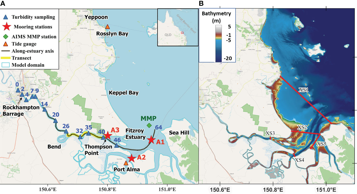
Figure 1 (A) Study site in the Fitzroy Estuary and Keppel Bay with long-term monthly turbidity profiling (dark blue) conducted by Department of Environment and Science (DES, QLD) since 2000; labelled with distance starting from the barrage (0 km) increasing seaward. Mooring station A1-A3 (red); Along-estuary axis (black); Survey transect (yellow) conducted in Nov 2022; Tidal gauge (orange) at Port Alma and Rosslyn Bay; Model domain (light blue); surface salinity and turbidity (2021-presesnt) collected at MMP (green) near estuary mouth by Australian Institute of Marine Science (AIMS); (B) Bathymetry data in 30m resolution obtained from Geoscience Australia; cross sections (XS1-XS5) for sediment flux calculation.
In this study, we focused on the seasonal characteristics of sediment being delivered to the GBR and the quantification of the sediment fluxes originating from the FE-KB catchment into the GBR, especially during major flood events. We used a systematic measurement-to-modelling framework to fill the following knowledge gaps:
1. How do different estuarine processes drive river-derived sediments from catchment to reef during both the dry and wet seasons?
2. What is the seasonal variability in the sediment budget?
3. How do estuary morphodynamics respond to seasonal variations in sediment transport?
We conducted a year-long field campaign, combined with long-term historical data and a numerical model, to understand wet-dry seasonal drivers of sediment transport and sediment budget in the FE-KB along the catchment-river-estuary-reef continuum. The model simulated a typical dry year (2022.01 – 06) and a wet year with a large flood event (2010.11 – 2011.03) in the FE-KB. Section 2 describes the field observation, model configuration and method used for sediment flux decomposition. In Section 3, we analyze the wet-dry seasonal variations of estuarine circulations and sediment characteristics from both field data and model results. Finally, we summarize the key findings of this study in the discussion and conclusion.
2 Methods
2.1 Study area
The Fitzroy Estuary (FE), located at ~23.5°S (see Figure 1), extends from a barrage at Rockhampton, ~70km from the coast and winds through low-lying agricultural catchments, finally discharges into Keppel Bay (KB) via southern deep channel. The FE-KB system in this study includes the upper FE (Barrage to Thompson Point), lower FE (Thompson Point to Sea Hill point, including southern tidal creeks) and KB (north of Sea Hill). Upstream of the barrage, the Fitzroy River (annual range of discharge 0 – 14,000 m3/s) drains a grazing dominated catchment area of about 142,000km2. Due to the catchment’s large size, there is a wide range of soil types, land cover characteristics, and rainfall-runoff dynamics, leading to climatic, hydrological, and geological differences between sub-catchments (Dougall et al., 2014; Huggins et al., 2017). Numerous studies have reported high level of sediment and nutrient loads from the catchment to the reef since European settlement (McCulloch et al., 2003; McKergow et al., 2005; Brodie et al., 2011). The current sediment load from the FE-KB catchment is estimated to have tripled due to increased land clearing and changes in land use since pre-European settlement (Kroon et al., 2012). The depositional history of the FE-KB system indicates that sediment from the river has accumulated in and around the lower FE (Thompson Point to Sea Hill) and the lower KB to form a more deltaic-type environment, characterized by extensive floodplain, salt flats, mangroves, and tidal creeks (Brooke et al., 2006; Ryan et al., 2006; Bostock et al., 2007).
The export of sediment from the FR is mainly controlled by highly episodic summer floods during wet months (November to March) and is redistributed primarily by tidal currents within the estuary and bay during the dry months (April to October) (Webster and Ford, 2010). The monthly-averaged hydrograph of FR (Figure 2) at the Gap (130005A, https://water-monitoring.information.qld.gov.au/) shows high seasonal and interannual variability in river flow due to the impact of El Nino and La Nina cycles. Generally, there are one or two above-mean annual flows, with the occasional large flood event lasting several weeks, and low flows for the remainder of the year. In 2022, the average discharge rate was 43 m3/s, with multiple flow events up to 1500 m3/s (Figure 2), indicating a relatively dry monitoring year. To assess sediment fluxes during a wet year, the model simulated the 2011 flood event, which caused severe flooding in January that lasted for about 18 days. This event set a record for the highest annual rainfall in the FR catchment and peak discharge rate exceeding 13,000 m3/s. The monitored FR catchment had an estimated annual total suspended solids load of nearly 7.0 Mt. y-1 in 2010-2011, with the fifth-highest flood peak recorded at 9.2m in Rockhampton.
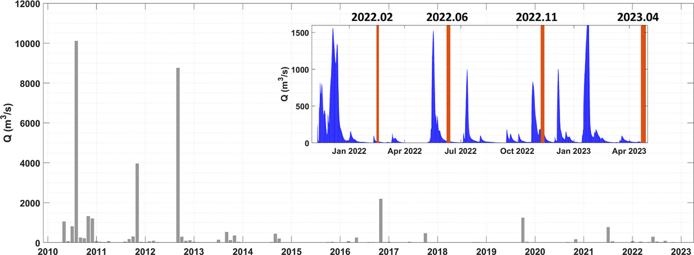
Figure 2 Monthly averaged river discharge since 2010 to present from the Fitzroy River measured at the Gap. Inset shows hourly river discharge in survey year 2022 with labels of four voyages (red).
The FE-KB system is tide-dominated with tidal range reaching 5m during spring tides and current speeds may exceed 1 ms-1 near the FE mouth. The system is well-mixed during the dry season, while during high river flow freshwater effectively flush the estuary and lower salinity in KB. It takes approximately 6-8 months for the salinity to increase back to marine levels (Herzfeld et al., 2005). Prior studies have shown a wide range of variations in salinity from the estuary head to the lower FE, which can range from being entirely fresh during river discharge pulses to being hypersaline throughout dry years (Webster and Ford, 2010). Port Alma in the lower FE was identified as the zone of maximum resuspension with a higher percentage of mud in surficial bottom sediments (Ryan et al., 2006; Webster and Ford, 2010).
Long term surface turbidity samples from the past 30 years (© State of Queensland (Department of Environment and Science) 2019) demonstrated the existence of a Turbidity Maximum Zone (TMZ) between stn.35 and stn.40 (refer to Figure 1 for stns labelled as distance from Rockhampton Barrage towards downstream). The turbidity levels are generally higher during the wet season, with greater mean and range, and lower at the seaward end of the estuary. TMZ is consistently higher during both wet and dry season compared to upstream and downstream regions (Figure 3).
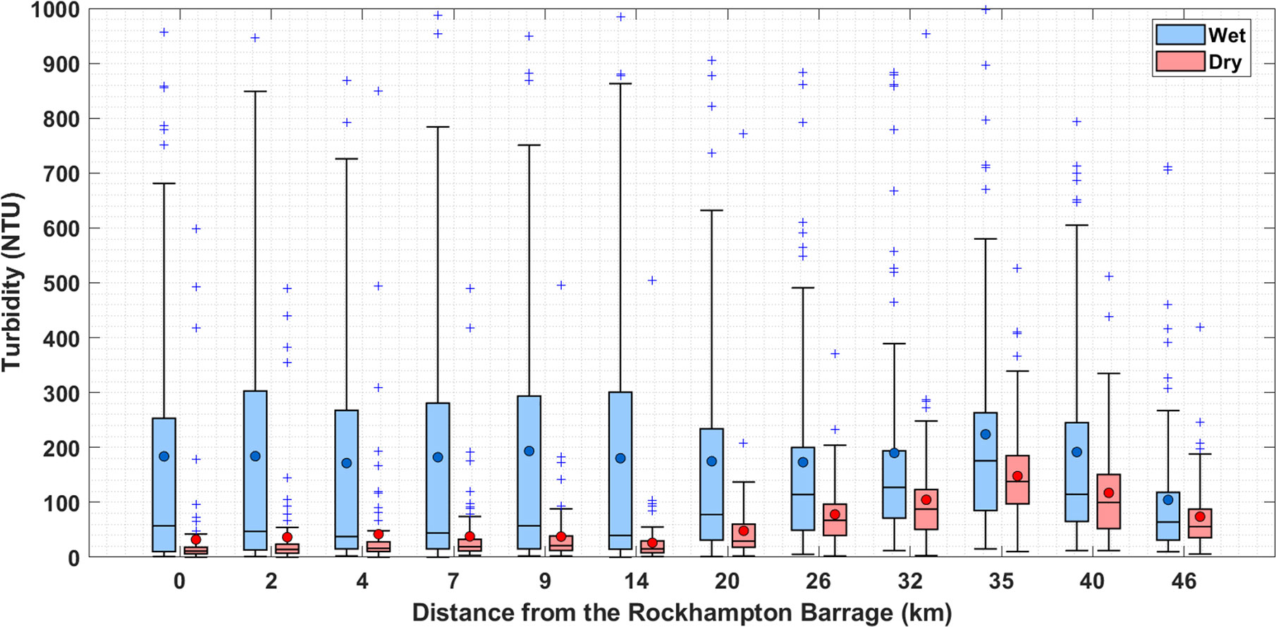
Figure 3 Boxplot of monthly surface turbidity samples along the Fitzroy River at 12 sites from 1993 to present during dry (red) and wet (blue) season. Boxes extend to interquartile range, the dot in each box is the mean value. Upper and lower whiskers extend to the 0.975 and 0.025 quantiles, respectively. Data collected by DES© State of Queensland (Department of Environment and Science) 2019.
2.2 In-situ observations
2.2.1 Spatial surveys
The four voyages were conducted in the FE in February, June, November 2022 and April 2023, each for one week. Spatial surveys were conducted to characterize the hydrodynamic conditions during two wet seasons (Feb, Nov) and two dry season (Apr, Jun). Due to weather conditions, the June 2022 survey was limited to the lower FE without access to the upper FE. All four surveys were conducted during spring tides. Surface water was continuously pumped to a series of flow-through cells submerged in an ambient water bath during each voyage. Flow-through measurements for temperature, salinity and turbidity were collected at 10-second intervals using a YSI EXO2 sonde. Continuous along-axis water-column profiles of salinity and temperature were collected in November 2022 while underway using small CTDs (Van Essen CTD-diver) and an electric reel following the methods of Crosswell et al. (2022). The profiling data were measured at 1-second intervals, as shown in Figure 1 (yellow line) for the along-axis transect in November 2022.
2.2.2 Fixed-point moorings
Two types of fixed-point stations were constructed, deployed and serviced during voyages. These three stations are denoted as “mooring stations” for distinction from other sampling stations. Two instrumented benthic lander frames were deployed at the estuary mouth (A1) and Port Alma (A2) to collect data continuously over tidal cycles from February 2022 for a one-year deployment. In June 2022, a telemetered mooring station (A3) was installed on a pylon near the border between the upper and lower estuary. The A3 station consisted of a side looking SonTek SL500 ADCP and a YSI EXO2 V2 sonde mounted about 1.5 m below mean low tide and a Vaisala weather Transmitter WXT520 weather station mounted about 8m above mean tide. The A3 station logged data at 10-minute intervals. At the A1 station, a Nortek signature 1000 ADCP and YSI EXO2 sonde were mounted about 0.5m above the seabed with a sampling interval of 10 minutes and a vertical cell size of 0.5m for the velocity profile. At the A2 station, a Nortek Aquadopp ADCP (1MHz) was mounted about 0.9m above the seabed with a sampling interval of 10 minutes and a vertical cell size of 1.0 m for the velocity profile. The YSI EXO2 sondes measured temperature, salinity, turbidity, pH, chl-a, DO and depth at 10-minute intervals and were calibrated immediately prior to deployment. Salinity and turbidity data from February – May 2022 at A2 is missing due to instrument failure.
Bottom boundary layer dynamics were measured using a bottom lander with a Nortek Vector ADV (16 MHz), LISST-100X and YSI EXO2 sonde mounted 15cm above the bed. The bottom critical shear stress for sediment erosion and deposition was measured to parameterize the sediment model. During the June and November voyages, the ADV lander was continuously deployed at three mooring sites for over 25hrs to capture full tidal cycles. The critical erosion stress for sediment was identified in the range of 0.1 – 0.2 kg·m-1s-2 for the sediment model configuration.
2.2.3 Discrete profiles and samples
Water-column profiles of in-situ turbidity and salinity were collected at the three mooring stations (A1 – A3) during each voyage. Meanwhile, 1L water samples were collected at the surface, mid-depth and bottom layers to derive the relationship between suspended sediment concentration (SSC, mg/L) and turbidity (FNU, which was found to be approximately SSC: Turbidity = 1.6:1 (R2 = 0.98, result shown in the supplement). These discrete water samples were collected over a period of ~47s using a peristaltic pump with the tube attached to the profiling cage near the EXO2 optical path.
Table 1 summaries the in-situ instrumentation, measured parameters and data acquisition periods at different locations. More information on observational data, e.g. Gantt charts for instrument deployments and other summary figures, is available in the data summary document and voyage reports that are part of the study data collection (Crosswell et al., 2023; https://doi.org/10.25919/chsj-pd27).
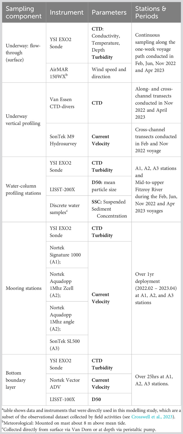
Table 1 Sampling equipment and methodsa.
2.2.4 Historical data
Time-series surface salinity and turbidity data in Fitzroy River mouth (Figure 1, MMP) were collected through in-situ monitoring by the Great Barrier Reef Marine Monitoring Program for Inshore Water Quality (MMP WQ, https://doi.org/10.25845/vr1c-0945). Sea-Bird Electronics SBE 37-SM were deployed 2m below the water surface at sampling interval of 10 minutes from 2021 to present.
2.3 Numerical model
The unstructured finite-volume community ocean model FVCOM, coupled with the UNSW-Sed module (Chen et al., 2003; Wang, 2002) was used to simulate the estuarine circulation and sediment dynamics in the FE-KB. The model domain covered ~50km offshore and ~60km upstream from the estuary mouth towards Rockhampton Barrage. The Rockhampton Barrage acts as a barrier to tidal and salt propagation, indicating the tidal limit of FE. Note that distances in this study are measured as downstream from the Rockhampton Barrage (Figure 1). The grid consisted of 40,930 nodes and 77,730 elements, with variable cell sizes ranging from ~2500m at the open ocean boundary down to 100m in the estuary (Figure 4). The vertical resolution was 20 sigma layers with higher resolution at the surface and bottom layers. The bathymetry data used was the high-resolution (30m) depth model for the GBR obtained from Geoscience Australia (Beaman, 2017).
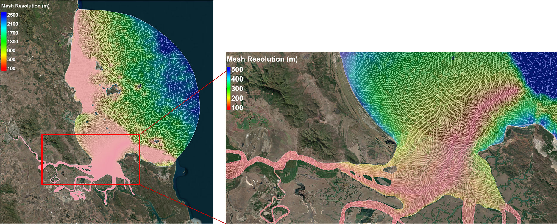
Figure 4 Model mesh resolution of the Fitzroy Estuary and Keppel Bay.
Open boundary conditions were specified by interpolating the dataset of tidal constituents from the TPX08 global tide model (Egbert and Erofeeva, 2002, https://www.tpxo.net/global/tpxo8-atlas, accessed Sep 2022) to the open boundary nodes. Catchment rainfall-runoff processes were simulated by GBR Dynamic SedNet model framework, which incorporates a paddock-scale pollutant generation model that calculates loads from rivers, side streams and creeks within the GBR catchments (Waters et al., 2014; Ellis, 2018; Waterhouse et al., 2018; McCloskey et al., 2021). The daily river discharge and sediment loads from the FR were added at the upstream boundary with salinity set to zero. The model was spun up for one month before the different model scenario runs with an initial zero velocity field and a uniform salinity field of 27 psu. The bottom drag coefficients is defined as 0.001m for marine bed and 0.0005 m for estuarine bed, time step for vertical diffusion is 0.4s and for horizontal advection is 2.0s.
The UNSW-Sed module was two-way coupled to the hydrodynamic model by allowing SSC to affect the seawater density and bottom drag coefficient (Wang, 2002). The detailed module algorithm can be found in the supplement. The parameters used in the sediment module are summarized in Table 2. Only one type of cohesive sediment is used in this study, of which the settling velocity is a function of suspended sediment concentration. It includes the flocculation and hindered settling process. Morphodynamics are simulated by calculating changes in bed thickness. The initial bed thickness is set to be 10m uniformly and reduced or increased by sediment erosion or deposition process.
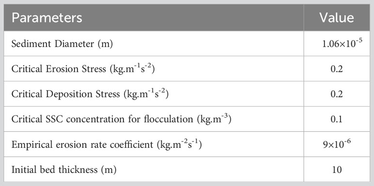
Table 2 Sediment model parameters.
Model scenarios with different river flow conditions combined with tidal forcing in barotropic and baroclinic modes were conducted (summarized in Table 3) to investigate the role of discharge magnitude on estuarine sediment transport (trapping and erosion) and the processes controlling the location of the TMZ.
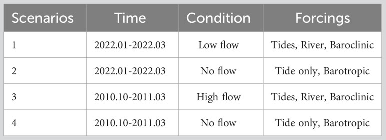
Table 3 Model scenarios.
2.4 Observational and model data analysis
Observational data of current velocity, salinity, and turbidity were grouped into wet and dry season data based on the presence of river flows (> 100 m3/s) within 10 days before data collection. These data were used to reveal the seasonal pattern in hydrodynamics and sediment transport, as well as possible drivers of seasonality in the FE-KB.
Simulated water surface elevation, salinity, SSC, and current velocity were compared with observation data to evaluate model performance, and calibration results are provided in the supplement. The model has the capability to predict the sediment flux along and across estuary within a defined area to provide a closed balance of sediment budget. The sediment flux was determined by integrating the product of water depth, SSC and current velocity at each layer along the cross-estuary or along-estuary transect, from the surface to the bottom. The resulting sediment flux was then separated into two components: mean advection (tidally averaged) and tidal pumping (tidally varying) components (McSweeney et al., 2016; Xiao et al., 2020). To calculate these components, the time series of SSC and principal velocity along -layer were low-pass filtered using a 36hr lanczos filter ( in the subscript is omitted for convenience):
where indicates the tidally averaged component and the remaining component; Fadv is the mean-advection component of sediment flux, Fpum is the tidal pumping component of sediment flux, and D is the total water depth. In the along-estuary direction, positive values indicate down-estuary transport, and negative values indicate up-estuary transport. The along-estuary and cross-estuary sediment flux were interpolated along the thalweg line and at the XS1 -XS5 transects at 100m intervals.
To evaluate the contributions by tidal and nontidal processes to the total sediment transport, the contribution (%) of mean advection and tidal pumping was calculated as follows:
Becherer et al. (2016) developed a close balance to decompose Fadv into barotropic and estuarine circulation components. They also used tidal averaging instead of the low-pass filter method, with the M2 tidal period as the averaging window. In their study, both methods were compared and found to agree well in reproducing the trend of sediment flux component variations, except for an unclosed balance in the previous method due to the omission of cross-correlation terms between mean velocity and fluctuating sediment concentration and vice versa. The estuarine circulation component is further extracted following Becherer et al. (2016):
The components calculated in Becherer et al. (2016) are in tidal-averaged and depth-mean format.
3 Results
3.1 Observational results
The main shipping channel is maintained at depths of 14m to 18m from the estuary mouth towards Port Alma (Figure 5A), resulting in strong tidal influence with high salinity (Figure 5B) and intermittent sediment resuspension due to strong tidal currents. Thompson Point (40 km) marks the rapid transition from deep and narrow (~16m deep and ~600m wide) to shallow and wide downstream (less than 10m deep and ~2000m wide; Figure 1). Moving upstream from Thompson Point toward the Bend (30 km) tidal motion gradually mixed saline water with freshwater. At the Bend, tidal currents and resuspension effects decreased, as was found in previous studies (Douglas et al., 2005; Webster et al., 2006). The area upstream from Bend to Rockhampton was dominated by the river with close-to-zero salinity and high turbidity throughout the study period. In Nov. 2022, the edge of the salt intrusion during rising tide was observed between Bend and Thompson Point about 32km from the Barrage. A classic two-layer structure of gravitational circulation was observed, with freshwater at the top and dense water at the bottom (Figure 5C).
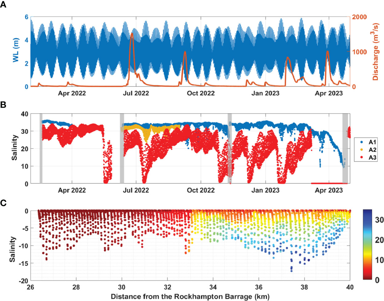
Figure 5 (A) Time series of water level at the Port Alma tide gauge (m), river discharge at the Gap (m3/s), and (B) salinity at three fixed-point mooring stations (A1 - A3, refer Figure 1 for locations). Grey shading indicates the time of four voyages; (C) Along-estuary transect of salinity profiles from CTD diver during rising tide on Nov 13th 2022.
The three mooring stations exhibited similar probabilities of exceeding depth-averaged current speeds, reaching a maximum of 1.5 m/s. The majority of current speeds (over 90%) remain below 1.0 m/s, or with the current speed exceeding 1.0 m/s less than 10% of the time (Figure 6A). A1 station stands out with an ebb-dominant asymmetric current, where over 10% of the ebb current exceeds 1.0 m/s during both the wet and dry seasons (Figures 6D, G). However, A3 station is located too close to the northern side of the riverbank to represent the main channel flow behaviour, which is not showing the flood-dominant tidal current that previous studies have predicted to induce the up-estuary pumping of sediment (Margvelashvili et al., 2003; Webster et al., 2003; Webster et al., 2006). The across-axis variability in current velocity was confirmed by ADCP transects in Nov 2022 using a SonTek M9 Hydrosurveyor (shown in supplement). In the survey year, A1 and A2 stations were not completely flushed fresh, with 80% of bottom salinity above 30 (Figure 6B). Conversely, A3 station experienced strong interactions between river discharge and tidal propagation, with 80% of bottom salinity above 8 and 18 during the wet and dry seasons, respectively (Figures 6E, H).
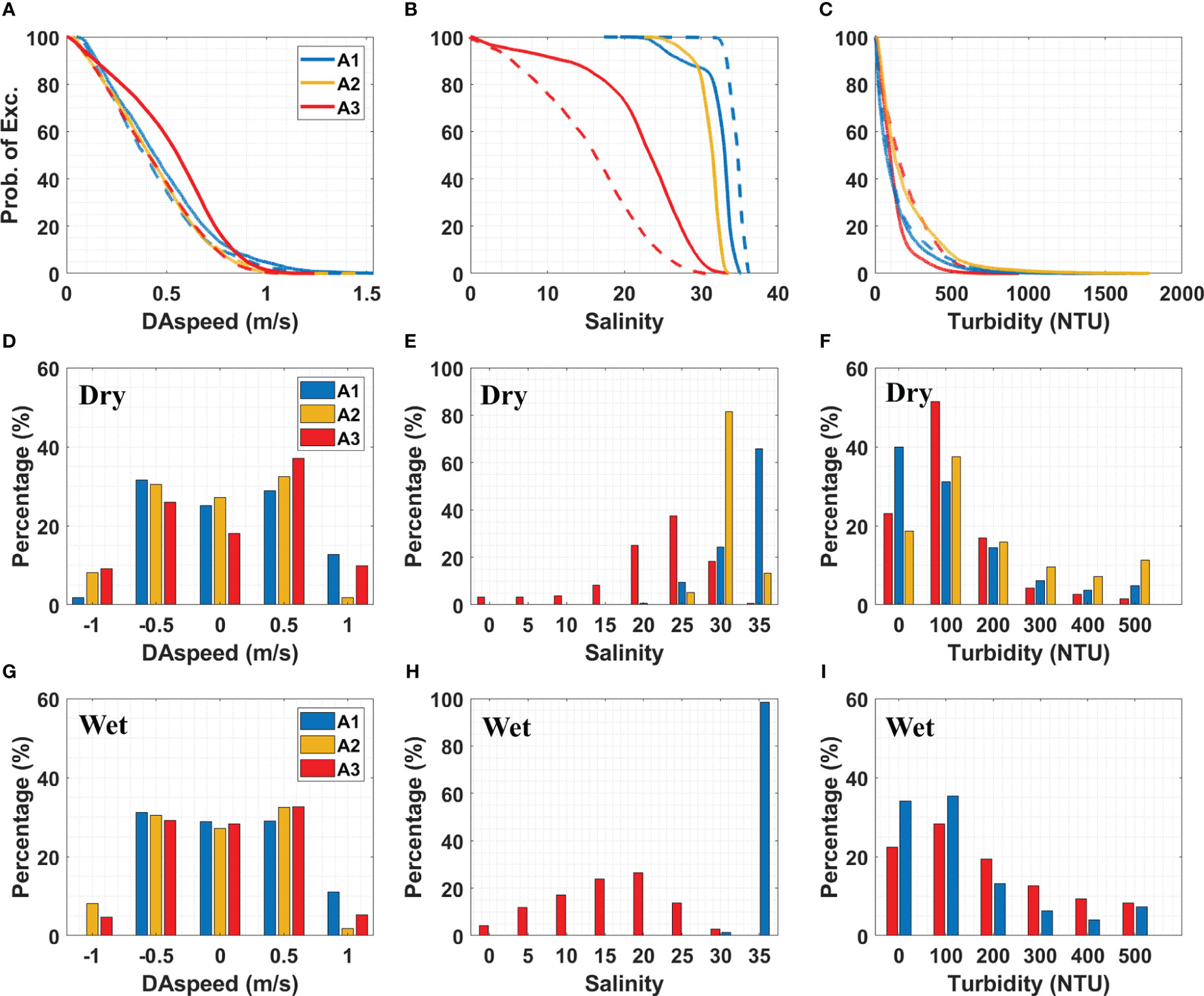
Figure 6 Probability (%) of depth-averaged velocity, bottom salinity and turbidity at A1 (blue), A2 (orange) and 1A3 (red). Exceedance plot (A–C) over dry season (solid) and wet season (dashed); Bar plot during dry season only (D–F); Bottom: Bar plot during wet season only (G–I); current speed: positive indicates ebb, negative indicates flood. 1A3 is a side looking ADCP and therefore values were the average of the 5 bins at the ADCP depth, which was oriented toward the opposing bank.
Bottom turbidity during the dry season shows a higher percentage of high values at Port Alma than at the other two stations (Figure 6F), though there is a lack of data for Port Alma during the wet season. A1 and A3 stations exhibit similar variation trends, with over 70% of the bottom turbidity during the dry season limited to 100 NTU, while high turbidity events are more common during the wet season (Figures 6C, F, I).
3.2 Modelling results
3.2.1 Numerical experiments on TMZ formation
Long-term in-situ turbidity data identified a TMZ between stn.35 and stn.40 (Figure 3), located in a deep hole upstream of Thompson Point. Two model scenarios were simulated and compared to investigate the effect of barotropic and baroclinic flows on TMZ formation during dry season (Jan-Mar. 2022). Scenario 1 had tides with low river flow in baroclinic mode, and scenario 2 had tides in barotropic mode only (Table 2). Figure 7 displays the vertical profile of three-month mean SSC, currents, and sediment fluxes from the Rockhampton Barrage (0 km) towards estuary mouth (64 km) in both scenarios. The SSC within the TMZ in scenario 1 (150-200 mg/L) was two to three times larger than in scenario 2 (50-100 mg/L), which showed a maximum SSC, consistent with the TMZ’s location observed from in-situ data (Figures 7A, E). The current profile in scenario 1 had a two-layer structure of surface seaward and bottom landward flow (Figure 7B), while scenario 2 showed vertically uniform seaward flow (Figure 7F). Sediment flux direction was consistent with the current profile, and the magnitude was much larger in scenario 1 (up to 25 g/s) than in scenario 2 (up to 5 g/s) due to the high SSC in scenario 1 (Figures 7C, G).
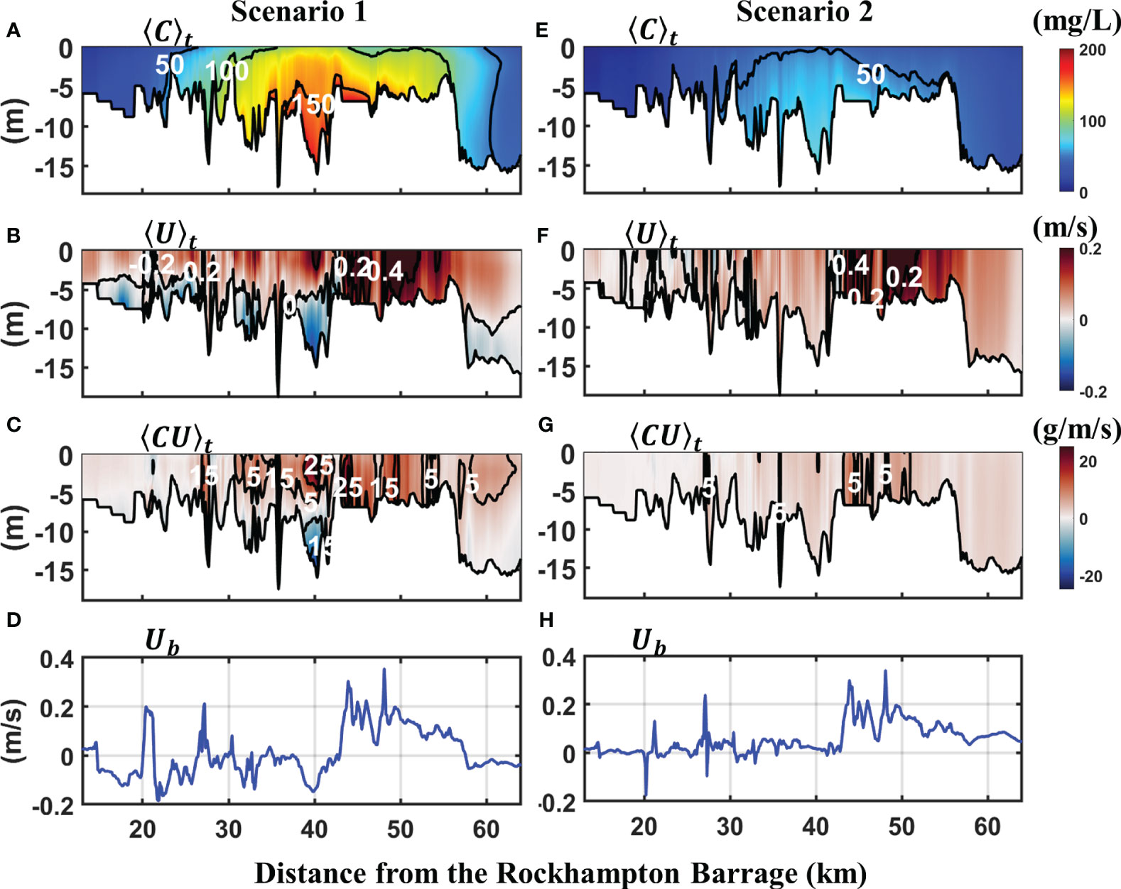
Figure 7 Simulated three-month mean (A, E) SSC (mg/L), (B, F) current (m/s), (C, G) sediment fluxes (g/m/s) and (D, H) bottom current along the thalweg line from the Rockhampton Barrage to estuary mouth in scenario 1 (left panel): tide plus river in baroclinic mode; scenario 2 (right panel): tide only in barotropic mode. Current/sediment flux: positive, down-estuary; negative, up-estuary.
In scenario 2, the existence of TMZ within the deep hole with tidal forcing only indicates its formation by barotropic flow under purely tide-topography interaction. It is not necessarily associated with the tide-river interaction or density gradient. The sharp transition of topography from approximately 17m deep to approximately 5m shallow near the Thompson Point causes sediment trapping within the deep hole, as observed in San Francisco Bay (Ganju and Schoellhamer, 2008). Increased water depth reduces bottom stress, leading to sediment deposition within the deep hole and creating a supply of easily erodible bottom sediment. Introducing baroclinic flow in scenario 1 increases bottom currents (Figure 7D), enhancing bottom stress for bed sediment erosion and local resuspension. Therefore, the enhanced SSC within the TMZ in scenario 1 is observed due to intensified bed erosion (Schoellhamer, 2000). As a result, the TMZ in scenario 1 under baroclinic flow is more significant than in scenario 2. The salinity profile from model shows average 26-28 within the TMZ (not shown here), so no evidence of TMZ formation driven by salt-freshwater interaction.
Overall, the topographic effect is the key mechanism for generating the TMZ in the deep hole upstream of Thompson Point. When the flow enters the deep hole, it slows down and changes direction, creating a convergence zone where sediment is deposited, leading to the formation of a sediment pileup with low flow condition. With time, this sediment pileup grows, resulting in the formation of a TMZ.
3.2.2 Effect of estuarine processes on sediment transport
In the scenario 1 with low flow condition, the deep hole within the TMZ shows consistent flood dominant flow, which is topographic effect induced inland residual current (|〈〈U〉t〉σ| < 0.1 m/s), while 〈〈C〉t〉σ fluctuates following spring-neap cycles (Figure 8A). Stronger tidal currents during spring tide contribute to sediment erosion and local sediment resuspension, resulting in a high concentration of sediment (〈〈C〉t〉σ > 200 mg/L).
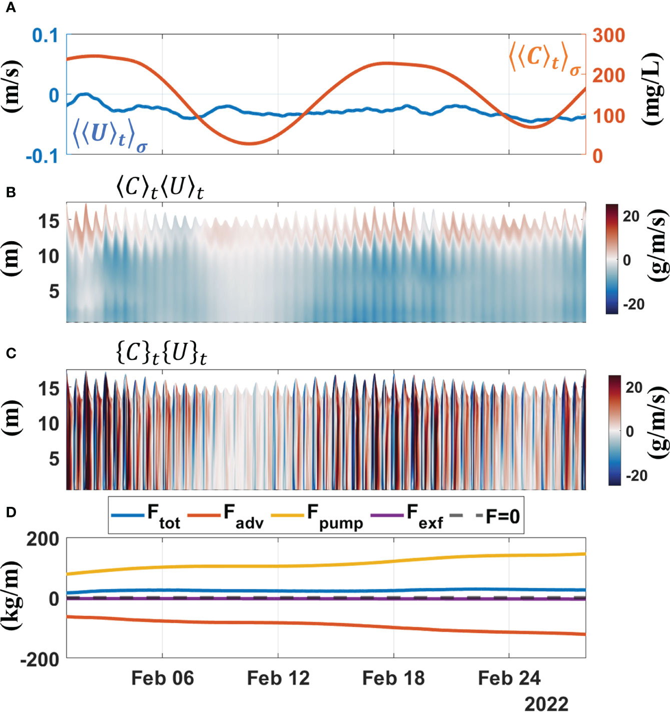
Figure 8 Sediment flux decomposition within TMZ in Scenario 1 (low flow), time window of 2022.02. (A) Depth-and tidally averaged currents along the estuary (m/s, blue) and SSC (mg/L, red); (B) mean-advection induced sediment flux (g/m/s); (C) tidal pumping induced sediment flux (g/m/s); (D) decomposed sediment flux (kg/m) accumulated since 2022.01, method used in Becherer et al. (2016).
The nontidal advective flux 〈C〉t〈U〉t shows two-layer vertical structure of surface seaward and bottom landward exchange flux (Figure 8B). 〈C〉t〈U〉t contains residual barotropic flux, caused by river runoff, barotropic ebb-flood asymmetries, and wind stress (not included in scenario 1), as well as a component purely driven by estuarine circulation (Becherer et al., 2016). Further decomposition was conducted following Becherer et al. (2016) to split the effects of residual barotropic flow and estuarine circulation.
The tidal pumping flux is the product of intertidal correlation between the tidal current and sediment concentration, which is driven by tidal fluctuations. shows an overall stronger magnitude than the advective flux, which is ebb-dominated.
To evaluate the key factors contributing to net sediment flux, sediment flux components were depth integrated. Sediment flux decomposition was conducted following Becherer et al. (2016), whereby Fexf (estuarine circulation component) was extracted from Fadv (nontidal advective component) to examine the impact of estuarine circulation, with remaining Fadv driven by barotropic flow. By integrating vertically, it becomes apparent that the net landward mean flux is mainly generated by mean advection Fadv, which is driven by flood-dominated residual currents. Fpump (tidal pumping component) indicates net down-estuary transport, as SSC peaks at ebb tides due to advective transport and turbulence generation (Figure 8C). Fexf becomes negligible (Figure 8D) as the system becomes well-mixed during low flow conditions. If tidal currents are the main engine for eroding sediment, one would expect a large sediment concentration during the flood tide due to the asymmetric flood-dominated current. During ebb, high SSC is advected from the river/TMZ, while the strong flood current brings low SSC. Thus, the sediment flux product indicates net down-estuary transport by tidal pumping. Overall, the tidal pumping component dominates the total net sediment flux in the deep hole within the TMZ, generating down-estuary sediment flux. Meanwhile, the flood-dominated residual currents, resulting from the topographic effect, generate up-estuary advective sediment flux, leading to sediment convergence within the TMZ.
Low flow condition (scenario 1) exhibited consistent sediment export along the estuary (Figure 9A), with the sediment transport decomposition revealing Fadv contributing to over 50% of sediment export (Figure 9B), except within the TMZ where it switched from sediment export to import. Fpump persistently drove sediment export along the estuary, with a dominant role within the TMZ, while Fexf had negligible contribution to Ftot. Furthermore, landward sediment flux by Fadv contributed to sediment convergence in the deep hole.
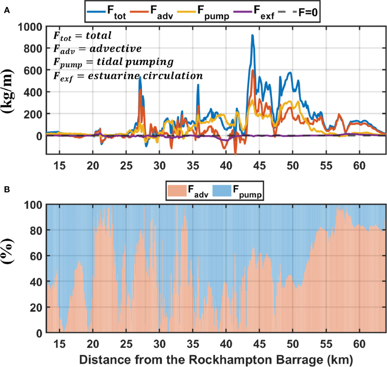
Figure 9 Along-estuary sediment flux in low flow condition (scenario 1). (A) sediment flux components (kg/m) accumulated over three months (2022.01-03), method used in Becherer et al. (2016); grey dashed line indicates the deep hole (DH) within TMZ; (B) percentage of sediment flux contribution by mean advection (Fadv) and tidal pumping (Fpump).
3.2.3 Changes to sediment trapping efficiency
The accumulated cross-channel sediment fluxes (XS1 – XS5, Figure 1) were used to evaluate the estuarine sediment trapping efficiency in the FE system during different river flow conditions (scenario 1&3, as shown in Table 2). XS2 represents the loads at the estuary mouth, while the SedNet model provides the catchment load. The estuarine trapping coefficient is calculated as follows:
where negative loads indicate import and positive loads indicate export. The additional sediment source in addition to the catchment loads received into the system is not included in the trapping coefficient.
During the 2011 event, the catchment’s sediment load reached 7.5 Mt, which is 4-5 times higher than the average annual input. Within three months after the event, the FE-KB system trapped around 2.4 Mt of sediment and exported 5.1 Mt (Table 4). The lower FE between XS1 and XS3 trapped 1.57 Mt of sediment, and an additional 0.53 Mt was delivered to the southern tidal creeks, with 0.3 Mt deposited within KB. Thus, the estuary trapped and redistributed approximately 28% of the catchment’s sediment load during the high flow event into the lower FE and southern tidal creeks.

Table 4 Accumulated sediment flux at each cross section and the estuarine sediment trapping coefficient.
During low flow conditions, sediment is brought in from offshore and from erosion in the upstream river catchment or channels and is deposited towards the lower FE and southern tidal creeks. The FE system functions as a sediment storage basin, with the capacity to trap 100% of the catchment loads and additional sediment source from offshore into the system. The efficiency of sediment trapping is negatively correlated with river discharge, as has been found in 15 other estuaries (Jay et al., 2007b), meaning that as river discharge decreases, the ability of the estuarine system to trap sediment increases.
3.2.4 Response of morphodynamics to river effect
The effect of river flow on the change of bed sediment thickness (erosion/deposition rate in mm/day, defined as ‘morphod’ in the supplement) is compared between scenario 3 (high river flow) and scenario 4 (no river flow) for the 2011 event (see Table 2). Morphod is calculated by dividing the accumulated change in bed sediment thickness by the event duration in both scenarios, as shown in Figure 10. In both scenarios, sediment erosion occurs consistently in the channel of the upper FE, with sediment deposition occurring near the bend (as also found in Ford (2006)), headlands and southern tidal creeks. During no river flow (Figure 10A), eroded sediments from the upper FE tend to accumulate near the Thompson Point (at the seaward border of the deep hole noted in Section 3.2.1) and the lower FE due to channel expansion. Bed erosion occurs at the Sea Hill and southern headland, where a deep channel is located with stronger ocean current intrusion. During high river flow (Figure 10B), both the upper FE and the accreted sandbars at the Thompson Point are eroded, with additional sediments from river flow. Sediments derived from the catchment and channel erosion will be redistributed and deposited within the lower FE, KB and the offshore area towards the north.
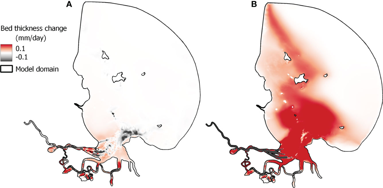
Figure 10 Mean sedimentation rate (mm/day) during the 2011 event: (A) Tide only (scenario 4); (B) high river flow (scenario 3); red indicates accretion; black indicates erosion.
Figure 11 shows bed sediment thickness change over 6 months (2010.10 – 2011.03) along the longitudinal thalweg line (Figure 1 black line) and cross-channel sections (XS1-XS5, Figure 1) in scenarios 3 (high river flow) and 4 (no river flow). The maximum erosion (up to 2m depth) occurs at the head of the upper FE due to strong river influence, gradually decreasing to 0.1m erosion depth at XS3 in scenario 3 (Figures 11C, F). Upper FE shows persistent erosion in both scenarios, but river flows significantly enhance the erosion rate. In contrast, lower FE and southern tidal creeks consistently deposit sediments, with<0.05m depth increase over 6 months (Figures 11B, D, E). As the channel expands from upper FE to lower FE, the current speed decreases, and sediment loads from the river tend to deposit. The prevailing offshore southwesterly current drives the sediment to deposit in the southern tidal creek. KB near the bay mouth (XS1) exhibits different trends, eroding under no river effect and depositing under high river flow effect (Figure 12A). When there is no strong river outflow, offshore currents bring sediments from the ocean into the FE-KB, causing channel erosion. However, when there is a high river flow, a large amount of sediment is flushed down from the river towards offshore, and sediment tends to deposit from the lower FE to outside the system.
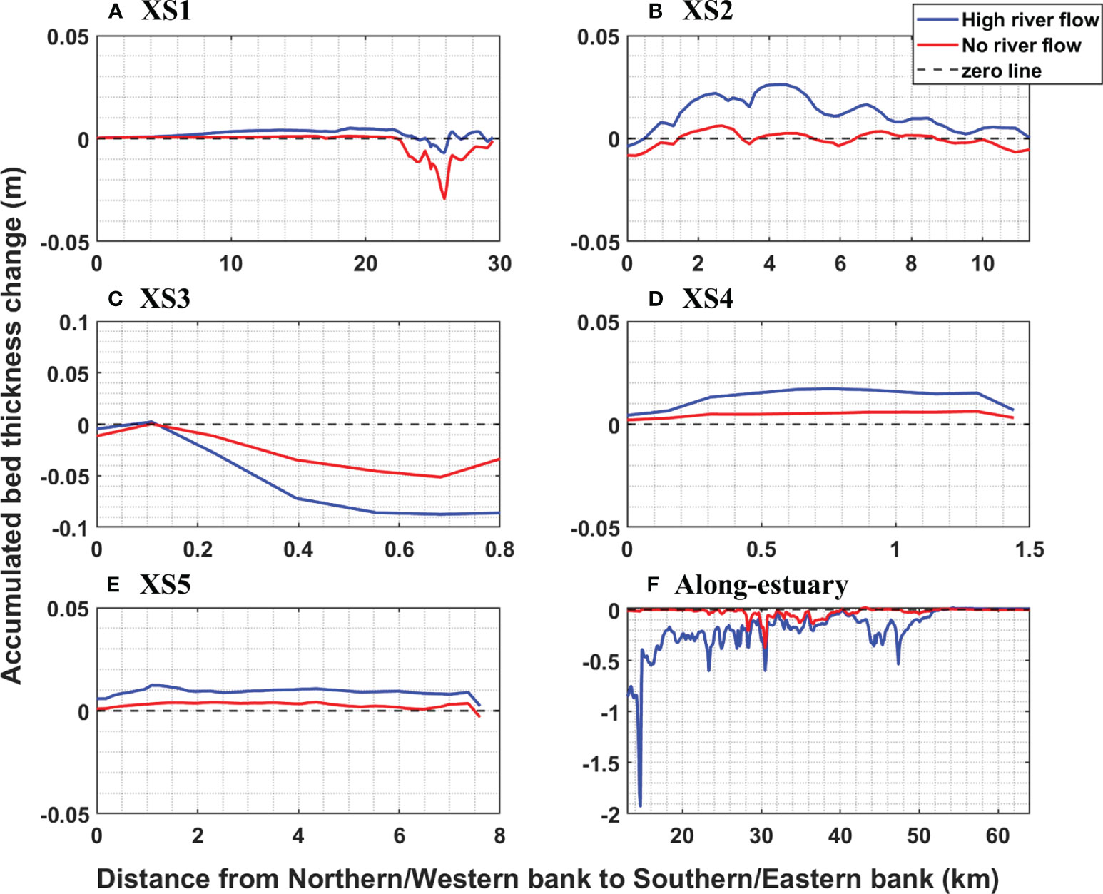
Figure 11 Accumulated variation on bed sediment thickness (m) during 2010.10 – 2011.03 in across-estuary sections (XS1 – XS5, A–E) and along-estuary section (F): red line, Tide only (scenario 4); blue line, high river flow (scenario 3).
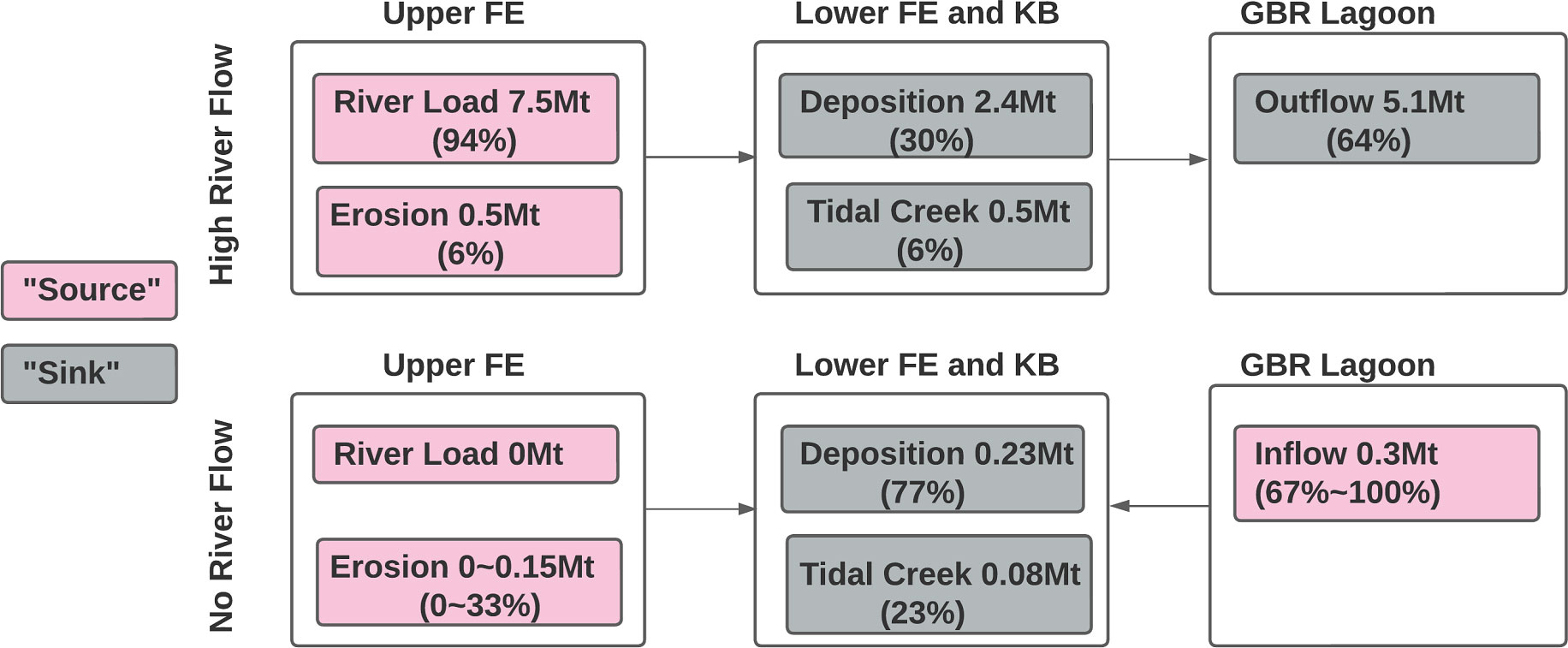
Figure 12 The sediment budget for the FE-KB during the period of 2010.10 – 2011.03 in high river flow (scenario 3) and no river flow (scenario 4).
4 Discussion
4.1 Implication on sediment budget calculations
Brooke et al. (2006) predicted sediment transport pathways and budgets for fine sediment (<63μm) based on sediment accumulation rates estimated from sediment cores in the FE-KB. The estimated catchment load for annual sediment (4.575 Mt y-1) used in sediment budget calculations by Brooke et al. (2006) is comparable to that of a wet year (2011) and two orders of magnitude greater than that of a dry year (2022). In Brooke et al. (2006), 55% of the annual average load was estimated to deposit within the estuary, with a large fraction deposited in mangroves (30%) and the lower FE (10%), including southern tidal creeks. The trapping coefficient over the past decades falls within the range reported in Table 3: 100% for a dry year and 28% for a wet year. Although our calculations indicate that the upper FE is consistently eroding during the model intervals, Brooke et al. (2006) estimated an accumulation of 8.6% within the same compartment. Asymmetric tidal currents were identified as the primary driver for net up-estuary transport (Webster and Ford, 2010), but this phenomenon was only observed within the TMZ and not within the upper FE in our study. Note that the model in this study does not include storage on the floodplain, mangroves and salt marshes, whereas the measured accumulation rates for the FE do include sedimentation in these areas and represent average accumulation over longer timescales. Besides catchment sources, offshore input can also be a crucial source of sediment for a river system, which was not reported in the study by Brooke et al. (2006). Our research has revealed that during low flow conditions, offshore influx can be transported to the system by currents and tides, resulting in a significant contribution to the sediment supply. Following a pulse of sediment export from the system into the offshore zone during a flood event, tidal, wind- and wave-driven currents tend to transport these river sediments back into the estuary where they are deposited in the lower FE and southern tidal creeks.
This study emphasizes the importance of considering the effect of seasonal variability in river flows on sediment accumulation rates when calculating the sediment budget for wet and dry seasons in the FE-KB. Similar modeling practices were conducted by Webster et al. (2006), who analyzed three single-year periods representing low (1993), medium (2003), and high (1999) river flow scenarios in the FE-KB. Both this study and Webster et al. (2006) revealed continuous channel erosion during low-medium flow conditions, however Webster et al. (2006) observed persistent export flux towards the GBR lagoon for all flow conditions. In this study, catchment loads were trapped within the system without export during low flow conditions. The updated sediment budget analysis in this study suggests that during dry seasons with low flow, sediment from catchment sources, channel erosion, and offshore sources tend to remain within the lower FE (64%), southern tidal creeks (23%), and KB (13%) (Figure 12). During wet seasons with high flow, sediment from catchment sources significantly outweighs channel erosion and offshore import. As a result, sediment accumulates in the lower FE (25%), southern tidal creeks (6%), and KB (5%). A considerable amount of sediment (64%) is also exported offshore during this season.
The drawback of calculating sediment budget estimated from sediment cores is its assumption of a long-term mean sediment delivery to the FE-KB system, without considering the variability in climate of sediment inputs. And it’s quite challenging to apply a mean estuarine trapping coefficient estimated from sediment cores to represent the trapping in the estuarine domain of GBR catchments, which is the current practice to determine trapping and erosion from catchment to reef. This study provides a framework for measuring and modeling sediment dynamics along the catchment-to-reef continuum, with the aim of more accurately estimating sediment budgets and estuarine trapping coefficients while taking into account estuarine processes and climate variability. The broader implication is that inputs to marine model from omitting estuarine processes in the catchments makes predicting, and most significantly, comparing the impact of catchment sediment-related water quality impairments tenuous. Livsey et al. (2022) stressed the importance of considering the complex interactions between catchment processes, riverine transport, estuarine dynamics, and reef ecosystem health when studying the catchment-to-reef continuum. They highlighted the differences in estuarine trapping coefficients across various GBR catchments and advocated for more comprehensive and integrated approaches to better understand and manage these ecosystems. By quantifying these interactions, effective strategies can be developed to protect and manage the GBR and other coastal ecosystems.
4.2 Limitation and future study
There are several limitations to this study that should be acknowledged. First, the study period was relatively short, covering only one wet year and one dry year. Future studies could extend the study period to capture interannual variability in sediment dynamics. Second, the study focused only on the effect of tidal forcing and river discharge on the morphological changes of the estuary and did not consider the impact of wind stress and wave-current interactions. Nevertheless, the development of a high-resolution model combined with high-resolution observations in this study advances our understanding of key drivers on sediment dynamics in the FE-KB, which have been previously observed and modelled at relatively coarse spatial and temporal scales.
Results from this study beget several recommendations for further research. First, the use of remote sensing data in combination with field measurements could improve model validation in the spatial domain, as remote sensing can provide snapshots of the entire model domain and even tidal time series in the case of geostationary satellites (Patricio-Valerio et al., 2022). However, in a highly turbid system like FE-KB, optical remote sensing may be limited to surface water and unable to resolve dynamic processes at depth, such as the TMZ observed in this study. Second, revision of long-term monitoring programs to include continuous, high-resolutions measurements at key FE locations, such as near Thompson Point downstream of the deep hole, could provide insights into the long-term trends and variability of sediment dynamics in the estuary. Third, the model is helpful on investigating the effects of future climate change on the sediment dynamics and morphology of the FE. Much of the coastal areas surrounding the FE is composed of low-relief salt flats and floodplains, and high-resolution modelling of sediment dynamics will be critical to predict and manage how this system responds to rising sea levels and more extreme weather in a changing climate. Finally, the model can be used and further developed for decision support, e.g. to inform future dredging and coastal development to promote actions that enhance sediment trapping efficiency within the FE rather than export to the GBR Lagoon.
5 Conclusions
This study used the measurement-to-modelling approach to analyze sediment dynamics in the Fitzroy Estuary – Keppel Bay in the Great Barrier Reef region. The one-year field campaign includes the collection of data on current speed, salinity and turbidity at three mooring stations and CTD profiles along-/cross- channels in the FE-KB. The in-situ measurements reveal the seasonal variation patterns on hydrodynamic and sediment dynamics, enabling us to better understand the dominant processes occurring in different regions of the system and to characterize the estuarine dynamics.
Both measurements and the model results confirm the existence of a TMZ in the deep hole near Thompson Point. Numerical experiments of barotropic and baroclinic forcings scenarios demonstrate that the key factor for TMZ formation is barotropic forcing under tide-topography interactions, while asymmetric tidal currents lead to sediment flux convergence. During low river flow, 100% of catchment loads and channel-eroded sediments in the upper FE will be stored in the lower FE and southern tidal creeks, with additional sediment sources from offshroe. However, with an increase in river flow, the estuarine trapping coefficient decreases to 20-30% of catchment loads, resulting in over 60% of the total sediment loads from both catchment and channel erosion being exported into the Great Barrier Reef.
The model results showed that river discharge plays a significant role in controlling sediment erosion and deposition patterns in the estuary. During high river flow, river flow increases sediment erosion and both the upper FE and the accreted sandbars in the TMZ are eroded and transported to the lower FE. During low river flow, sediment deposition is dominant and sediment accumulates within the TMZ and the lower FE. The study also found that the upper FE is more susceptible to sediment erosion within a range of 0.1m – 2m over a 6-months period due to its topographic restriction to the Thompson Point and the strong river influence. However the lower FE and southern tidal creek act as sediment storage basins for deposition, with less than 0.05m of deposition. The sediment dynamics in the Fitzroy Estuary were complex and varied along the estuary, highlighting the importance of considering spatial variability in estuarine sediment dynamics.
The study provides valuable insights into the formation on TMZ, seasonality of sediment dynamics and the role of river flow in shaping the estuary’s morphology. These findings can have implications for the management and conservation of other estuaries that are subject to similar environmental conditions.
Data availability statement
The datasets presented in this study can be found in online repositories. The names of the repository/repositories and accession number(s) can be found below: https://doi.org/10.25919/ka99-xy66.
Author contributions
ZX, AS, JC and DL contributed to conception and design of the study. ZX, JC, GC and AS conducted field data collection and data management. DS contributed knowledge on modelling and DL contributed knowledge on monitoring technics. ZX and JC performed data analysis. ZX wrote first draft of manuscript. AS, JC, DL and DS contributed to manuscript review. All authors contributed to the article and approved the submitted version.
Funding
The authors declare financial support was received for the research, authorship, and/or publication of this article. This research was supported by Commonwealth of Scientific and Industrial Research Organization (CSIRO), funded by eReefs project – a public-private collaboration between Australia’s leading operational and scientific research agencies, government, and corporate Australia. The funder was not involved in the study design, collection, analysis, interpretation of data, the writing of this article, or the decision to submit it for publication.
Acknowledgments
We benefited from insightful discussion and input from Dr. Zoe Bainbridge and Dr. Stephen Lewis from James Cook University and Professor Xiao Hua Wang from UNSW Canberra. Observation data at MMP station were collected as part of the Fitzroy Basin Marine Monitoring Program for Inshore Water Quality, which is funded by the partnership between the Australian Government’s Reef Trust and the Great Barrier Reef Foundation, and the Australian Institute of Marine Science. Department of Environment Science (DES) contributes to the GBR Dynamic SedNet model framework paddock and catchment modelling. We are grateful for DES sharing long-term turbidity data in the system (Based on or contains data provided by the State of Queensland (Department of Environment and Science) 2019). We are thankful for field assistance from John Robert, Gemma Kerrisk from CSIRO Environment and High-Performance Computing cluster help from Peter Campbell from CSIRO IM&T. The model simulations have been carried out on the CSIRO Petrichor HPC cluster.
Conflict of interest
The authors declare that the research was conducted in the absence of any commercial or financial relationships that could be construed as a potential conflict of interest.
Publisher’s note
All claims expressed in this article are solely those of the authors and do not necessarily represent those of their affiliated organizations, or those of the publisher, the editors and the reviewers. Any product that may be evaluated in this article, or claim that may be made by its manufacturer, is not guaranteed or endorsed by the publisher.
Supplementary material
The Supplementary Material for this article can be found online at: https://www.frontiersin.org/articles/10.3389/fmars.2023.1215161/full#supplementary-material
References
Bainbridge Z., Lewis S., Bartley R., Fabricius K., Collier C., Waterhouse J., et al. (2018). Fine sediment and particulate organic matter: A review and case study on ridge-to-reef transport, transformations, fates, and impacts on marine ecosystems. Mar. Pollut. Bull. 135, 1205–1220. doi: 10.1016/j.marpolbul.2018.08.002
Baird M. E., Mongin M., Skerratt J., Margvelashvili N., Tickell S., Steven A. D. L., et al. (2021). Impact of catchment-derived nutrients and sediments on marine water quality on the Great Barrier Reef: An application of the eReefs marine modelling system. Mar. Pollut. Bull. 167, 112297. doi: 10.1016/j.marpolbul.2021.112297
Beaman R. J. (2017). High-resolution depth model for the Great Barrier Reef - 30 m. (Geoscience Australia: Canberra). doi: 10.4225/25/5a207b36022d2
Becherer J., Flöser G., Umlauf L., Burchard H. (2016). Estuarine circulation versus tidal pumping: Sediment transport in a well-mixed tidal inlet. J. Geophysical Research: Oceans 121 (8), 6251–6270. doi: 10.1002/2016jc011640
Bostock H. C., Brooke B. P., Ryan D. A., Hancock G., Pietsch T., Packett R., et al. (2007). Holocene and modern sediment storage in the subtropical macrotidal Fitzroy River estuary, Southeast Queensland, Australia. Sedimentary Geology 201 (3-4), 321–340. doi: 10.1016/j.sedgeo.2007.07.001
Brodie J.E., Devlin M., Haynes D., Waterhouse J. (2011). Assessment of the eutrophication status of the Great Barrier Reef Lagoon (Australia). Biogeochemistry 106, 281–302. doi: 10.1007/s10533-010-9542-2
Brodie J., Kroon F., Schaffelke B., Wolanski E., Lewis S., Devlin M., et al. (2012). Terrestrial pollutant runoff to the Great Barrier Reef: an update of issues, priorities and management responses. Mar. Pollut. Bull. 65, 81–100. doi: 10.1016/j.marpolbul.2011.12.012
Brooke B., Bostock H., Smith J., Ryan D. (2006). “Geomorphology and sediments of the Fitzroy River coastal sedimentary system - Summary and overview,” in Cooperative Research Centre for Coastal Zone Estuary and Waterway Management, technical report, Vol. 47. (Cooperative Research Centre for Coastal Zone, Estuary and Waterway Management (Coastal CRC)). Available at: http://ozcoasts.org.au/wp-content/uploads/pdf/CRC/47_geomorph_sediment_overview_screen.pdf.
Carroll C., Waters D., Vardy S., Silburn D. M., Attard S., Thorburn P. J., et al. (2012). A Paddock to reef monitoring and modelling framework for the Great Barrier Reef: Paddock and catchment component. Mar. Pollut. Bull. 65 (4-9), 136–149. doi: 10.1016/j.marpolbul.2011.11.022
Chen C., Liu H., Beardsley R. C. (2003). An unstructured grid, finite-volume, three-dimensional, primitive equations ocean model: application to coastal ocean and estuaries. J. Atmos. Ocean Technol. 20 (1), 159–186. doi: 10.1175/1520-0426(2003)020<0159:AUGFVT>2.0.CO;2
Crosswell J. R., Bravo F., Pérez-Santos I., Carlin G., Cherukuru N., Schwanger C., et al. (2022). Geophysical controls on metabolic cycling in three Patagonian fjords. Prog. Oceanography 207. doi: 10.1016/j.pocean.2022.102866
Crosswell J. R., Carlin G., Steven A. (2019). Controls on carbon, nutrient, and sediment cycling in a large, semiarid estuarine system; princess charlotte bay, Australia. J. Geophysical Research: Biogeosciences 125 (1). doi: 10.1029/2019jg005049
Crosswell J. R., Carlin G., Xiao Z. (2023). Suspended sediment, hydrodynamic, and biogeochemical observations in Fitzroy Estuary - Keppel Bay Region, QLD 2022-2023; an eReefs sediment dynamics study Vol. v4 (CSIRO Australia: CSIRO. Data Collection). doi: 10.25919/ka99-xy66
Dougall C., Ellis R., Shaw M., Waters D., Carroll C. (2014). Modelling reductions of pollutant loads due to improved management practices in the Great Barrier Reef catchments – Burdekin NRM region, Technical Report 4. (Queensland Department of Natural Resources and Mines, Rockhampton, Queensland). Available at: https://wetlandinfo.des.qld.gov.au/resources/static/pdf/ecology/catchment-stories/lower-burdekin/dougall2014.pdf.
Douglas G., Ford P., Moss A., Noble B., Packett B., Palmer M., et al. (2005). “Carbon and nutrient cycling in a subtropical estuary (the Fitzroy), Central Queensland,” in Cooperative Research Centre for Coastal Zone Estuary and Waterway Management, technical report, Vol. 14. (Cooperative Research Centre for Coastal Zone, Estuary and Waterway Management (Coastal CRC)). Available at: https://www.researchgate.net/publication/228110700_Carbon_and_nutrient_cycling_in_a_subtropical_estuary_the_Fitzroy_Central_Queensland.
Egbert G. D., Erofeeva S. Y. (2002). Efficient inverse modeling of barotropic ocean tides. J. Atmospheric Oceanic Technol. 19 (2), 183–204. doi: 10.1175/1520-0426(2002)019<0183:EIMOBO>2.0.CO;2
Ellis R. J. (2018).Dynamic SedNet Component Model Reference Guide: Update 2017. Concepts and algorithms used in Source Catchments customisation plugin for Great Barrier Reef catchment modelling. (Bundaberg, Queensland: Queensland Department of Environment and Science).38, pp. Available at: https://www.publications.qld.gov.au/dataset/dynamic-sednet-reference-guide.
Ford P. W. (2006). Nutrient dynamics and sediment budgets in the Fitzroy estuary during a flood event : a report to the Fitzroy Basin Association Inc / P.W. Ford (CRC Coastal Zone Estuary and Waterway Management).
Furnas M. (2003). Catchments and Corals: Terrestrial Runoff to the Great Barrier Reef (Queensland: Australian Institute of Marine Science), 334. pp.
Ganju N. K., Schoellhamer D. H. (2008). “Chapter 24 Lateral variability of the estuarine turbidity maximum in a tidal strait,” in Proceedings in marine science, vol. 9 . Eds. Kusuda T., Yamanishi H., Spearman J., Gailani J. Z. (Elsevier), 339–355. doi: 10.1016/S1568-2692(08)80026-5
Ganti V., Chadwick A. J., Hassenruck-Gudipati H. J., Fuller B. M., Lamb M. P. (2016). Experimental river delta size set by multiple floods and backwater hydrodynamics. Sci. Adv. 2 (5), e1501768. doi: 10.1126/sciadv.1501768
Garzon-Garcia A., Wallace R. L., Huggins R., Turner R. D., Smith R. A., Orr D. N., et al. (2015). Total suspended solids, nutrient and pesticide loads (2013–2014) for rivers that discharge to the Great Barrier Reef – Great Barrier Reef Catchment Loads Monitoring Program. Department of Science, Information Technology and Innovation. Brisbane. Downloaded from https://pure.coventry.ac.uk/ws/portalfiles/portal/11981178/2013_2014_gbr_catchment_loads_technical_report.pdf.
Herzfeld M., Andrewartha J. R., Sakov P., Webster I. (2005). “Numerical hydrodynamic modelling of the Fitzroy Estuary,” in Cooperative Research Centre for Coastal Zone Estuary and Waterway Management, technical report, Vol. 38. (Cooperative Research Centre for Coastal Zone, Estuary and Waterway Management (Coastal CRC)). Available at: http://hdl.handle.net/102.100.100/176174?index=1.
Huggins R., Wallace R., Orr D. N., Smith R. A., Taylor O., King O. C., et al (2017). Total suspended solids, nutrient and pesticide loads (2015–2016) for rivers that discharge to the Great Barrier Reef . Great Barrier Reef Catchment Loads Monitoring Program. Queensland Department of Environment and Science. Available at: https://www.reefplan.qld.gov.au/__data/assets/pdf_file/0028/45991/2015-2016-gbr-catchment-loads-technical-report.pdf.
Jay D. A., Orton P. M., Chisholm T., Wilson D. J., Fain A. M. V. (2007). Particle trapping in stratified estuaries: Application to observations. Estuaries Coasts 30 (6), 1106–1125. doi: 10.1007/BF02841400
Jones A. M., Berkelmans R. (2014). Flood impacts in Keppel Bay, southern great barrier reef in the aftermath of cyclonic rainfall. PLoS One 9 (1), e84739. doi: 10.1371/journal.pone.0084739
Kroon F. J., Kuhnert P. M., Henderson B. L., Wilkinson S. N., Kinsey-Henderson A., Abbott B., et al. (2012). River loads of suspended solids, nitrogen, phosphorus and herbicides delivered to the Great Barrier Reef lagoon. Mar. Pollut. Bull. 65 (4-9), 167–181. doi: 10.1016/j.marpolbul.2011.10.018
Lewis S., Bartley, Packett R., Dougall C., Brodie J., Bartley R., et al. (2015). “Fitzroy Basin Association, issuing body,” in Fitzroy sediment story: a report for the Fitzroy Basin Association, report No.15/74. (Rockhampton, Qld: Fitzroy Basin Association). Available at: http://nla.gov.au/nla.obj-3033400947, Retrieved April 2, 2023.
Livsey D. N., Crosswell J. R., Turner R. D. R., Steven A. D. L., Grace P. R. (2022). Flocculation of riverine sediment draining to the Great Barrier Reef, implications for monitoring and modeling of sediment dispersal across continental shelves. J. Geophysical Research: Oceans 127, e2021JC017988. doi: 10.1029/2021JC017988
Margvelashvili N., Andrewartha J., Baird M., Herzfeld M., Jones E., Mongin M., et al. (2018). Simulated fate of catchment-derived sediment on the Great Barrier Reef shelf. Mar. Pollut. Bull. 135, 954–962. doi: 10.1016/j.marpolbul.2018.08.018
Margvelashvili N., Herzfeld M., Webster I. (2006). “Modelling of fine-sediment transport in the Fitzroy Estuary and Keppel Bay,” in Cooperative Research Centre for Coastal Zone Estuary and Waterway Management, technical report, Vol. 39. (Cooperative Research Centre for Coastal Zone, Estuary and Waterway Management (Coastal CRC)). Available at: http://ozcoasts.org.au/wp-content/uploads/pdf/CRC/39_fine_sediment_fitzroy_keppel.pdf.
Margvelashvili N., Robson B., Sakov P., Webster I., Parslow J., Herzfeld M., et al. (2003). “Numerical modelling of hydrodynamics, sediment transport and biogeochemistry in the Fitzroy Estuary,” in Cooperative Research Centre for Coastal Zone Estuary and Waterway Management, technical report, Vol. 9. (Cooperative Research Centre for Coastal Zone, Estuary and Waterway Management (Coastal CRC)). Available at: https://www.researchgate.net/publication/228110704_Numerical_modelling_of_hydrodynamics_sediment_transport_and_biogeochemistry_in_the_Fitzroy_Estuary.
McCloskey G., Baheerathan R., Dougall C., Ellis R., Bennett F. R., Waters D., et al. (2021). Modelled estimates of fine sediment and particulate nutrients delivered from the Great Barrier Reef catchments. Mar. Pollut. Bull. 165, 112163. doi: 10.1016/j.marpolbul.2021.112163
McCulloch M, Fallon S, Wyndham T, Hendy E, Lough J, Barnes D. (2003). Coral record of increased sediment flux to the inner Great Barrier Reef since European settlement. Nature 421 (6924), 727–30. doi: 10.1038/nature01361
McKergow L. A., Prosser I. P., Hughes A. O., Brodie J. (2005). Sources of sediment to the great barrier reef world heritage area. Mar. Pollut. Bull. 51 (1-4), 200–211. doi: 10.1016/j.marpolbul.2004.11.029
McSweeney J. M., Chant R. J., Sommerfield C. K. (2016). Lateral variability of sediment transport in the delaware estuary. J. Geophys. Res.: Oceans 121 (1), 725–744. doi: 10.1002/2015JC010974
Packett R. (2017). Rainfall contributes ~30% of the dissolved inorganic nitrogen exported from a southern Great Barrier Reef river basin. Mar. Pollut. Bull. (2017) 121, 16–31.
Patricio-Valerio L., Schroeder T., Devlin M. J., Qin Y., Smithers S. (2022). A machine learning algorithm for himawari-8 total suspended solids retrievals in the great barrier reef. Remote Sens. 14 (14). doi: 10.3390/rs14143503
Robson B., Webster I., Margvelashvili N., Herzfeld M. (2006). Scenario modelling: simulating the downstream effects of changes in catchment land use. (Cooperative Research Centre for Coastal Zone, Estuary and Waterway Management (Coastal CRC)). Vol. 41. Available at: http://hdl.handle.net/102.100.100/174677?index=1.
Ryan D., Brooke B., Bostock H., Collins L., Siwabessy P. J., Margvelashvili N., et al. (2006). Geomorphology and sediment transport in Keppel Bay, central Queensland, Australia. Cooperative Research Centre for Coastal Zone, Estuary and Waterway Management (Coastal CRC). Vol. 49. Available at: https://www.researchgate.net/publication/253326735_Geomorphology_and_sediment_transport_in_Keppel_Bay_central_Queensland_Australia.
Schoellhamer D. H. (2000). “Influence of salinity, bottom topography, and tides on locations of estuarine turbidity maxima in northern San Francisco Bay,” in Proceedings in Marine Science, vol. 3 . Eds. McAnally W. H., Mehta A. J. (Elsevier), 343–357. doi: 10.1016/S1568-2692(00)80130-8
Steven A. D. L., Baird M. E., Brinkman R., Car N. J., Cox S. J., Herzfeld M., et al. (2019). eReefs: An operational information system for managing the Great Barrier Reef. J. Operational Oceanography 12 (sup2), S12–S28. doi: 10.1080/1755876x.2019.1650589
Steven A. D. L., Baird M., Crosswell J., Carlin G., Kenna E., Rochester W., et al. (2020). “Continuous monitoring and model parameterisation of estuarine water quality entering the great barrier reef,” in CSIRO Final Report to Great Barrier Reef Foundation. (CSIRO technical report) 84, pp. Available at: https://www.researchgate.net/publication/344990040_Continuous_Monitoring_and_Model_Parameterisation_of_Estuarine_Water_Quality_entering_the_Great_Barrier_Reef.
Turner R., Huggins R., Wallace R., Smith R., Vardy S., Warne M. (2012). Sediment, nutrient and pesticide loads: Great Barrier Reef Loads Monitoring 2009-2010. (Brisbane: Department of Science, Information Technology, Innovation and the Arts). Available at: https://www.reefplan.qld.gov.au/__data/assets/pdf_file/0027/45981/2009-2010-gbr-catchment-loads-report.pdf..
Turner R., Huggins R., Wallace R., Smith R., Vardy S., Warne M St. J. (2013). Total suspended solids, nutrient and pesticide loads, (2010-2011) for rivers that discharge to the Great Barrier Reef Great Barrier Reef Catchment Loads Monitoring 2010-2011 Department of Science. (Brisbane: Department of Science, Information Technology, Innovation and the Arts). Available at: https://www.reefplan.qld.gov.au/__data/assets/pdf_file/0028/45982/2010-2011-gbr-catchment-loads-report.pdf.
Wallace R., Huggins R., King O., Gardiner R., Thomson B., Orr D. N., et al. (2016). Total suspended solids, nutrient and pesticide loads, (2014–2015) for rivers that discharge to the Great Barrier Reef – Great Barrier Reef Catchment Loads Monitoring Program. (Brisbane: Department of Science, Information Technology, Innovation and the Arts). Available at: https://www.reefplan.qld.gov.au/__data/assets/pdf_file/0035/45989/2014-2015-gbr-catchment-loads-technical-report.pdf.
Wallace R., Huggins R., Smith R. A., Turner R. D. R., Garzon-Garcia A., Warne M., et al. (2015). Total suspended solids, nutrient and pesticide loads, (2012–2013) for rivers that discharge to the Great Barrier Reef – Great Barrier Reef Catchment Loads Monitoring Program 2012–2013. (Brisbane: Department of Science, Information Technology, Innovation and the Arts). Available at: https://www.reefplan.qld.gov.au/__data/assets/pdf_file/0031/45985/2012-2013-gbr-catchment-loads-technical-report.pdf.
Wallace R., Huggins R., Smith R., Turner R., Vardy S., Warne M., et al. (2014). Total suspended solids, nutrient and pesticide loads, (2011–2012) for rivers that discharge to the Great Barrier Reef – Great Barrier Reef Catchment Loads Monitoring Program 2011–2012. (Brisbane: Department of Science, Information Technology, Innovation and the Arts). Available at: https://www.reefplan.qld.gov.au/__data/assets/pdf_file/0029/45983/2011-2012-gbr-catchment-loads-report.pdf.
Walsh J. P., Nittrouer C. A. (2009). Understanding fine-grained river-sediment dispersal on continental margins. Mar. Geology 263 (1), 34–45. doi: 10.1016/j.margeo.2009.03.016
Wang X. H. (2002). Tide-induced sediment resuspension and the bottom boundary layer in an idealized estuary with a muddy bed. J. Phys. Oceanogr. 32 (11), 3113–3131. doi: 10.1175/1520-0485(2002)032<3113:TISRAT>2.0.CO;2
Waterhouse J., Henry N., Mitchell C., Smith R., Thomson B., Carruthers C., et al. (2018). Paddock to reef integrated monitoring, modelling and reporting (paddock to reef) program design 2018-2022. State of Queensland: Tech. rep.). Available at: https://www.reefplan.qld.gov.au/__data/assets/pdf_file/0026/47249/paddock-to-reef-program-design.pdf.
Waters D. K., Carroll C., Ellis R., Hateley L., McCloskey G. L., Packett R., et al. (2014). Modelling reductions of pollutant loads due to improved management practices in the Great Barrier Reef catchments – Whole of GBR, Technical Report. (Brisbane: Queensland Department of Natural Resources and Mines). Available at: https://www.reefplan.qld.gov.au/__data/assets/pdf_file/0029/45983/2011-2012-gbr-catchment-loads-report.pdf.
Webster I., Atminskin I., Bostock H., Brooke B., Douglas G., Ford P., et al. (2006). The Fitzroy Contaminants Project - A study of the nutrient and fine-sediment dynamics of the Fitzroy Estuary and Keppel Bay. (Cooperative Research Centre for Coastal Zone, Estuary and Waterway Management (Coastal CRC)). Available at: http://hdl.handle.net/102.100.100/174523?index=1.
Webster I. T., Ford P. W. (2010). Delivery, deposition and redistribution of fine sediments within macrotidal Fitzroy Estuary/Keppel Bay: Southern Great Barrier Reef, Australia. Continental Shelf Res. 30 (7), 793–805. doi: 10.1016/j.csr.2010.01.017
Webster I., Ford P., Robson B., Margvelashvili N., Parslow J. S. (2003). Conceptual models of the hydrodynamics, fine sediment dynamics, biogeochemistry and primary production in the Fitzroy Estuary. (Cooperative Research Centre for Coastal Zone, Estuary and Waterway Management (Coastal CRC)). Available at: https://ozcoasts.org.au/wp-content/uploads/2016/03/8-fitzroy_conceptual_models.pdf.
Wenger A. S., Williamson D. H., da Silva E. T., Ceccarelli D. M., Browne N. K., Petus C., et al. (2016). Effects of reduced water quality on coral reefs in and out of no-take marine reserves. Conserv. Biol. 30 (1), 142–153. doi: 10.1111/cobi.12576
Keywords: sediment budget, numerical model, in situ observation, highly turbid estuary, catchment to reef
Citation: Xiao Z, Carlin G, Steven ADL, Livsey DN, Song D and Crosswell JR (2023) A measurement-to-modelling approach to understand catchment-to-reef processes: sediment transport in a highly turbid estuary. Front. Mar. Sci. 10:1215161. doi: 10.3389/fmars.2023.1215161
Received: 01 May 2023; Accepted: 27 September 2023;
Published: 18 October 2023.
Edited by:
João Miguel Dias, University of Aveiro, PortugalCopyright © 2023 Xiao, Carlin, Steven, Livsey, Song and Crosswell. This is an open-access article distributed under the terms of the Creative Commons Attribution License (CC BY). The use, distribution or reproduction in other forums is permitted, provided the original author(s) and the copyright owner(s) are credited and that the original publication in this journal is cited, in accordance with accepted academic practice. No use, distribution or reproduction is permitted which does not comply with these terms.
*Correspondence: Ziyu Xiao, YW1hbmRhLnhpYW9AY3Npcm8uYXU=
†ORCID: Daniel N. Livsey, orcid.org/0000-0002-2028-6128