A review of mechanically stimulated bioluminescence of marine plankton and its applications

Bioluminescence is ubiquitous in marine ecosystems and found in uni- and multicellular organisms. Bioluminescent displays can be used to deter predators, attract mates, and lure and hunt prey. Mechanically stimulated flash kinetics of zooplankton and dinoflagellates are life stage-dependent and species-specific, and could prove effective at identification and monitoring biodiversity in bioluminescent species. Here, we provide a comprehensive review of mechanically stimulated bioluminescence for the main dinoflagellate and zooplankton clades in marine environments and assemble known flash kinetics and spectral emission data. Instruments and methods used in measuring bioluminescence are also discussed. Applications, research gaps, perspectives, and biases in approaches to studying bioluminescence are identified. Moreover, emission kinetics of most zooplankton are very poorly known and constitute a critical gap. Lastly, available knowledge is interpreted in terms of potential future changes in global bioluminescence driven by climate change.

1 Introduction

Bioluminescence is a widespread mode of communication in marine environments. Lau and Oakley (2021) estimated that bioluminescence evolved at least 94 times across all taxa and is present in at least 760 genera (Herring, 1987; Haddock et al., 2010). Considering bioluminescent organisms are taxonomically widespread and present in most marine ecosystems (Lapota and Losee, 1984; Martini and Haddock, 2017), understanding its drivers, functions, and diversity is imperative and relevant to marine biologists, ecologists, and physical and biological oceanographers alike. Bioluminescence can be stimulated chemically by a change in water pH by adding specific chemicals, electrically by applying a voltage to the water volume, or mechanically by disturbing the flow (Hamman and Seliger, 1972; Herring, 1981). Mechanical stimulation is achieved when hydrodynamic external forces, e.g., waves, eddies, feeding currents of filtering organisms, etc., exert local stress on the cellular membrane, enabling an action potential and the bioluminescent chemical reaction to occur (Deane and Stokes, 2005). This review is focused solely on mechanically stimulated bioluminescence of marine planktonic organisms.

Mechanically stimulated bioluminescence (MSB) can often be seen on beaches with breaking waves, or in the wake of a moving ship or swimming nekton. As in all luminescent organisms, light emission is caused by a chemical reaction in specialized organelles or cells with the substrate luciferin catalyzed by the enzyme luciferase. Several different types of luciferin exist and vary between and within phyla (see Haddock et al. (2010) and Widder (2010a) for a taxonomic breakdown of chemical diversity). Euphausiids and dinoflagellates both use dinoflagellate luciferin. Cnidarians, ctenophores, some ostracods, copepods, decapod shrimps, chaetognaths, and larvaceans all use coelenerazine as their luciferin. Cypridina luciferin is found only in cypridinid ostracods and the midshipman fish Porichthys, their predator (Haddock et al., 2010). Every luciferin, when oxidized in a chemical reaction mediated by a corresponding luciferase, will emit at a wavelength spectrum that is unique to the luciferin and accessory proteins, thus resulting in varying spectral properties across bioluminescent organisms (Wilson and Hastings, 2012). Emissions may be further spectrally filtered by cellular contents and/or tissues.

Figure 1 shows a typical first flash response of the dinoflagellate Pyrocystis fusiformis, obtained through mechanical stimulation in the Underwater Bioluminescence Assessment Tool (UBAT; SeaBird Electronics, Bellevue, WA). For those organisms able to flash multiple times, the first flash is usually most intense. Since the kinetics associated with the first emission are often species-specific (Nealson et al., 1986; Johnsen et al., 2014), they have potential for differentiating between species in situ. Typical flash kinetic parameters for an individual organism are generally the peak intensity (PI) in photons/s, the rise time (RT) in ms, the decay time (DT) in ms, the flash duration (FD) in ms, and the first flash of mechanically stimulated light (FF-MSL) in photons/flash. The peak intensity is measured as the highest instantaneous intensity during the first flash. The rise time is measured as the time between the first emission above baseline to the peak intensity. Similarly, the decay time is measured from the peak intensity to its return to baseline. The flash duration is measured as the time at which emissions are above baseline for a single emission. It is also equal to the sum of RT and DT. FF-MSL is the total amount of photons emitted in a single flash, based on the time period established by the flash duration. FF-MSL and often other kinetic parameters are highly dependent on the applied shear level, physiological state of the organism, and the instrument used for measurement (Latz and Rohr, 2013). The e-folding time (EF, in ms) is the time needed for the decaying emission intensity to reach 1/e of the maximum intensity, starting from the emission peak timestamp. For bathyphotometer mechanically stimulated light (BP-MSL) and total mechanically stimulable light (TMSL), we follow the descriptions of Latz and Rohr (2013). BP-MSL is defined as the average bioluminescence intensity measured in a specific bathyphotometer (photons/s), but is more specifically expressed in photons/s/L when taking into account the bathyphotometer’s chamber volume and flow rate. This parameter or similar derived parameters have been used to characterize a water system based on MSL and to uncover associated seasonal and spatial variations in emission capacity (see Section 5 for ecological applications). Importantly, BP-MSL is instrument-specific since every bathyphotometer has different incident shear stresses affecting the MSL and its flash kinetics. Additionally, residence times for organisms in a photometer measurement cavity vary between sensors, so measurements can only be effectively compared when using the same instrument (more detail provided in Section 3). TMSL is typically determined in a controlled laboratory setting and can be described as the total amount of mechanically stimulated light (or luminescence) for a single individual or cell under maintained stimulation until light emission exhaustion, with units photons/cell or photons/ind. Bioluminescence potential (BP) is the absolute maximal amount of photons that can be produced by an organism, typically measured through acid treatment and is expressed in photons/cell or photons/ind. This is the terminology that will be used to discuss kinetics, as there are significant inconsistencies in the literature (see Section 6).

Figure 1

Figure 1 Typical first flash emission of the dinoflagellate Pyrocystis fusiformis obtained with the UBAT, with annotated flash kinetics. (A) Peak intensity (PI). (B) Rise time (RT). (C) Decay time (DT). (D) Flash duration (FD). (E) First flash of mechanically stimulated light (FF-MSL). See text for details.

Herein, we discuss current knowledge and gaps for MSB of dinoflagellates and the main zooplankton clades. We outline the various functions attributed to biologically emitted light and discuss what is known regarding the role of MSB. We provide an extensive and updated review of MSB flash kinetics of several species measured over the past few decades. Since several hundred bioluminescent species exist, we discuss every major planktonic group of interest for which flash kinetics were measured, or at least discussed. For a comprehensive inventory of bioluminescent species, we recommend the works of Esaias and Curl (1972); Herring (1983); Poupin et al. (1999), and Widder et al. (1983). We then describe multiple instruments used to study MSB in laboratory conditions and in situ. The scientific applications in ecology, diversity, oceanography, climate change, autonomous sensing, and other fields are explored. Finally, we identify gaps in the literature regarding bioluminescence research and provide an assessment of the biases that can occur when collecting data on bioluminescent organisms. This effort builds upon previous reviews and research by Haddock et al. (2010); Herring (1983); Latz et al. (1988); Marcinko et al. (2013b); Martini and Haddock (2017); Moline et al. (2013); Widder et al. (1983), and Widder (2010a), with a focus on zooplankton and dinoflagellate clades. Key objectives are to assess remaining gaps, to evaluate the potential for bioluminescence as a tool to study diversity, and to identify pathways forward for research and technology development.

2 Bioluminescence emissions in plankton

MSB in marine species is thought to enhance survivability by luring or finding prey and warding off predators (Haddock et al., 2010). MSB can either be intrinsic, semi-intrinsic or extrinsic (Mirza and Oba, 2021). Intrinsic bioluminescence occurs when an organism produces both the luciferin and the luciferase needed for the chemical reaction. Inversely, an organism that obtains these molecules through predation and diet will display extrinsic bioluminescence. An individual with semi-intrinsic bioluminescence will obtain one of the components through their diet, sometimes facultatively.

Bioluminescence is present in at least 14 phyla, most having marine species (Morin, 1983; Widder, 2002). In some groups such as cnidarians, nearly all described species produce light (Martini and Haddock, 2017). Since the ability to bioluminesce seems to have evolved several times (Haddock et al., 2010; Lau and Oakley, 2021), one can expect significant variability in ecological value and emission flash kinetics from one group to another and within species. In the following section, we discuss emission characteristics, functions, and ecology of bioluminescence for the main clades of zooplankton and dinoflagellates.

2.1 Dinoflagellata

Dinoflagellates are autotrophic, heterotrophic, or mixotrophic single-cell organisms that are abundant in coastal and open ocean environments in the photic zone. They are known for their bioluminescent displays along the shore, i.e., Noctiluca scintillans and Lingulodinium polyedra, and some species are responsible for toxic red tides, i.e., Karenia brevis, Pyrodinium bahamense, and L. polyedra (Fleming et al., 2011). Haddock et al. (2010) and Poupin et al. (1999) counted at least 18 genera of bioluminescent dinoflagellates in five orders (Gymnodiniales, Noctilucales, Peridiniales, Prorocentrales, and Pyrocystales). Marcinko et al. (2013b) reviewed a total of 68 species of confirmed bioluminescent dinoflagellates. Because of their ecological role and the possibility to keep clonal cultures in laboratory, the bioluminescence of dinoflagellates has been extensively studied since the 1950s (Haxo et al., 1955). Indeed, first flash kinetics of several species have been characterized (Widder and Case, 1981; Latz and Lee, 1995; Cussatlegras and Le Gal, 2005; Cussatlegras and Le Gal, 2007), and their response to shear stress has been measured in fully developed pipe flow and other characterized flow fields (Latz et al., 2004b; Maldonado and Latz, 2007; Watanabe et al., 2012).

Bioluminescence emissions originate from scintillons, organelles containing the luminescent chemistry that are activated by a pH change following deformation of the plasma membrane, i.e., mechanical stimulation (Figure 2). This deformation is usually caused by a flow gradient present in the water column, i.e., shear, originating from waves, currents, other organisms swimming close by, or the feeding current of a predator. Dinoflagellates have a species-specific shear stress threshold, below which they will not typically bioluminesce. Peak bioluminescence emissions and TMSL typically exhibit a graded response to shear stress levels, i.e., higher shear stress typically produces a higher bioluminescence intensity (Latz et al., 1994; Latz and Rohr, 1999; Maldonado and Latz, 2007). Latz et al. (2004b) found that the shear stress threshold for four species of dinoflagellates varied from 0.02 to 0.3 N/m² with fully developed pipe flow experiments. Species where shear-induced bioluminescence has been studied include L. polyedra (Anderson et al., 1988; Dassow et al., 2005), Pyrocystis noctiluca (Cussatlegras and Le Gal, 2004), Pyrocystis lunula, (Jarms et al., 2002; Cussatlegras and Le Gal, 2007; Watanabe et al., 2012), P. bahamense (Biggley et al., 1969), Ceratocorys horrida (Latz and Lee, 1995; Latz et al., 2004a), Gonyaulax spinifera (Vishal et al., 2021), and Tripos fusus (Latz et al., 2004b), although thresholds have rarely been established. Table 1 summarizes the shear stress thresholds of available species along with the method or instrument used to quantify it. Shear stress thresholds for bioluminescence also vary between coastal or open ocean species (Marcinko et al. (2013b); coastal species tend to have higher thresholds, presumably because they live in a high-energy environment, which prevents unnecessary energetic expenditure.

Figure 2

Figure 2 Mechanically stimulated bioluminescence in the dinoflagellate Pyrocystis fusiformis. Photo courtesy of Iyvone Khoo.

Table 1

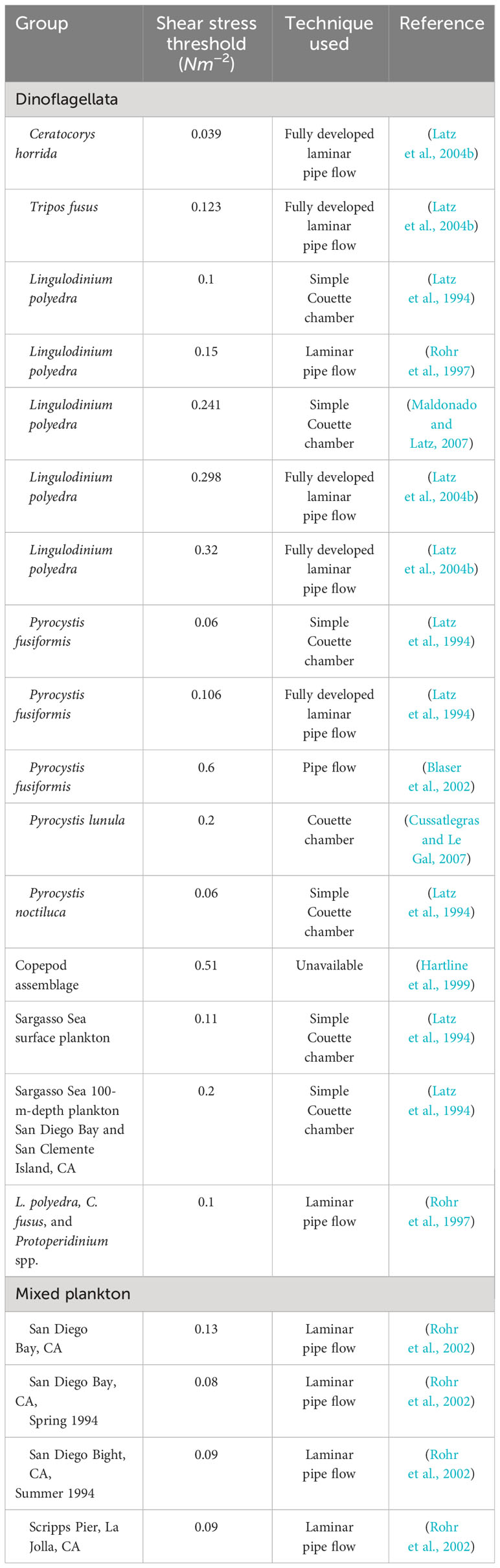
Table 1 Shear stress thresholds for dinoflagellates and zooplankton, along with the method used for quantifying the shear levels.

Flash kinetics of dinoflagellates vary by several orders of magnitude among different species. For example, FF-MSL was 2.50 × 10¹¹ photons/flash for N. scintillans using mechanical stimulation in an integrating light chamber (Buskey et al., 1992) and 3.35 × 10⁸ photons/flash for P. bahamense using mechanical stimulation through stirring and bubbling (Biggley et al., 1969). Indeed, TMSL varies based on organism size and the ability to produces several flashes repeatedly (Biggley et al., 1969). There is a positive correlation between TMSL of dinoflagellates and cell surface area; indeed, the approximate ratio of 10¹¹ photons mm⁻² is referred to as Seliger’s rule (Buskey et al., 1992). When mechanically stimulated, the rise time of dinoflagellates is usually less than 50 ms, shorter than most other bioluminescent phyla (Widder, 1991; Latz and Lee, 1995). Widder and Case (1981) observed that P. fusiformis produces two types of flashes when mechanically stimulated for prolonged periods, where the second flash is dimmer and longer in both duration and rise time. Changes in flash responses upon repeated stimulation appear to be a feature of Pyrocystis species (Tesson and Latz, 2015). Other dinoflagellate species likely can produce variable flash kinetics upon secondary stimulation. Mean emission wavelengths for dinoflagellate species vary from 471 to 480 nm (Widder et al., 1983; Latz and Lee, 1995; Poupin et al., 1999). Emitted wavelength maxima are highly conserved across different genera of dinoflagellates, which is not the case for other phyla (Section 2.9).

Three primary roles for MSB in dinoflagellates have been hypothesized to enhance survival. The first function is likely to startle predators with a bright and rapid flash when entrained in a feeding current. Dinoflagellate cultures displaying brighter bioluminescence emissions were less preyed upon by the copepod Acartia tonsa (White, 1979). Esaias and Curl (1972) measured reduced ingestion rates by copepods on dinoflagellate cultures with higher bioluminescence potential. The swimming patterns of copepods are also altered in the presence of bioluminescent flashes caused by dinoflagellates, appearing as a startle response that can be interpreted as a fleeing behavior from a predator that would be attracted by this light (Buskey et al., 1983). This second function is described as the burglar alarm hypothesis, in which a dinoflagellate flash will cause the copepod to jump away to possibly avoid any visual predator that could capture it. Dinoflagellate bioluminescence reduced their predation by the mysid Holmesimysis costata via secondary predation by fish on H. costata (Mesinger and Case, 1992). Cusick and Widder (2014) and Hanley and Widder (2017) provided nuance to this theory in comparing bright and dim dinoflagellates and their ability to deter predators by flashing. Their results suggest that flashes of dimmer species like Alexandrium spp. and L. polyedra will hinder predator grazing (via secondary predation), but only above a certain cell concentration. This was not the case for brighter species, e.g., P. fusiformis, where this effect can be attained at high and low cell concentrations. The third function for dinoflagellate MSB is thought to be aposematism. In these cases, the bright blue flashes would act as a colorful warning to predators of the toxic nature of that particular species (Hanley and Widder, 2017).

For a predator, ingesting a flashing dinoflagellate is also risky, since light emitted from the digestive gut of the predator can alert other predators. Considering entire populations of some dinoflagellates are clones of a single organism, ingestion by a predator is not always detrimental to the population (Abrahams and Townsend, 1993). Thus, the cost of losing a few individuals may in fact be tolerable to the clonal colony, making bioluminescence a viable strategy to enhance survival of the population.

Some species of dinoflagellates can significantly contribute to the bioluminescence of a given ecosystem. For example, up to 30% of the bioluminescence measured at stations in the Sargasso Sea was caused by P. noctiluca (Swift et al., 1985). This is due both to the bright flashes it creates and its abundance in the water column when conditions allow. Under bloom conditions, which may be highly persistent in locations such as the bioluminescent bays of Puerto Rico, the dinoflagellate P. bahamense can completely dominate bioluminescence (Sastre et al., 2013; Soler-Figueroa and Otero, 2016). N. scintillans is a major contributor to bioluminescence from tropical oceans to northern seas, and is often responsible for red tide events, causing fish and invertebrate mortality through rapid eutrophication creating hypoxic conditions (Zahir et al., 2023). Chen et al. (2023) measured decreasing bioluminescence intensity with increasing salinity and temperature, but intensity remained unchanged with varying levels of nutrients. See Marcinko et al. (2013b) for a more complete discussion on the applications and modeling of dinoflagellate bioluminescence emissions and their relative contributions to the water column’s bioluminescence.

2.2 Arthropoda

2.2.1 Copepoda

Copepods are one of the most abundant invertebrate clades in marine and freshwater systems, both in biomass and abundance (Le Borgne, 1982; Webber and Roff, 1995; Blaxter et al., 1998). They are an important link between primary production and higher trophic levels such as larval fish and macroinvertebrates. Although the most abundant species are not bioluminescent, several copepod species of ecological importance are bioluminescent (Herring, 1988) and can be important proxies for secondary production estimates and ecosystem health assessments.

The majority of bioluminescent copepods are in the Augaptilidae, Heterorhabdidae, Lucicutiidae, and Metridinidae families, though several species belonging to other families have been documented (Clarke et al., 1962; Herring, 1988; Takenaka et al., 2012). Copepods do not have light-producing organs sensu stricto, e.g., photophores. Instead, luciferin-luciferase-mediated light emissions are produced in glandular cells, for which the quantities and locations are highly variable among species (Herring, 1988). Light-emitting gland contents are usually excreted out of pores into the water column, although some species retain light emission in the glands. The latter is the case for the calanoid Oncaea conifera displaying peak emissions of 6.90×10⁸ photons/s/ind on average (mechanically stimulated through stirring in an integrating sphere) (Herring et al., 1993). M. lucens has been shown to synthesize all needed components for bioluminescence emissions, i.e., intrinsic bioluminescence, but it is believed that most copepods acquire at least one of the compounds (luciferin/luciferase) through predation (Mirza and Oba, 2021). Light-producing cells of copepods have been found in a small cluster on the head between the antennules, on the ventral side, on the exopods of swimming legs, and on the caudal rami (Clarke et al., 1962; Takenaka et al., 2017). Peak emission wavelengths for planktonic copepods range from 469 to 492 nm (Herring, 1983; Takenaka et al., 2012; Santhanam, 2022). Some species will not excrete clouds of bioluminescent secretions and light will be constrained to the glands.

The main function for bioluminescent displays by copepods is antipredatory. By secreting luminescent fluids into the water column or by quickly flashing, copepods presumably hope to distract, disorient, and cloud the vision of predators long enough for them to be able to produce a swimming burst and escape (Porter and Porter, 1979; Hartline et al., 1999). Indeed, the well-studied copepod Metridia lucens will only flash on its own, i.e., without mechanical or chemical stimulation, when in the presence of the predator, Meganyctiphanes norvegica presumably from visual and chemical recognition (David and Conover, 1961). M. lucens may also flash to alert other individuals of potential danger, essentially acting as an alert system (Buskey and Swift, 1985). Copepods are also thought to use MSB as a “burglar alarm” as previously mentioned for dinoflagellates, as the planktonic polycheate Tomopteris septentrionalis showed increased swimming speeds when M. lucens flashed, perhaps to reduce their own predation (Buskey and Swift, 1985). For freshwater copepods, however, no change in behavior can be observed when bioluminescent flashes are present (Buskey et al., 1987), showing potentially different ecological roles in different environs.

Consistent with the taxonomic and morphological diversity of copepods, the flash kinetics of bioluminescence emissions, when described, are highly variable. With flashes of 0.2 to 30 s in duration for M. lucens, copepods can produce some of the longest flashes of all crustacean zooplankton (Herring, 1988). Among the brightest is the centimeter-long calanoid Gaussia princeps living in temperate and tropical waters. This copepod can sustain PI emissions at 483 to 488 nm for up to 3 s, resulting in a very high TMSL (4.30×10¹¹ photons/ind measured through mechanical stimulation in an integrating sphere) (Barnes and Case, 1972; Widder et al., 1983; Latz et al., 1990). According to Bowlby and Case (1991), PI for this species averaged 3.5×10¹⁰ photons/s, and the FF-MSL was estimated at 1.8×10¹¹ photons/ind when measured in an integrating sphere. However, results showed that four types of flash responses can be obtained via electrical stimulation, i.e., one with relatively fast rise time, one with a long total duration, one with a slow rise time and long duration, and a compound emission with a fast or long flash followed by a slow flash.

Species with very broad distributions can display large variations in kinetics. Indeed, for Oncaea conifera stimulated in an integrating sphere, Herring et al. (1993) noted significantly longer RT and FD for the North American population (64.9 ms and 213 ms, respectively) compared to the Mediterranean population (26.2 ms and 88.5 ms, respectively), although no statistical differences were observed for PIs and FF-MSLs. Similar results were obtained by Latz et al. (1987a) when studying the copepod Pleuromamma xiphias. With PI of 3.32×10¹¹ photons/s (Latz et al., 1990), three different sets of flash kinetics and peak emissions were obtained when mechanically stimulating at three different shear levels, i.e., fast rise and decay, slow rise and decay, and a compound flash of a fast and a slow flash (Latz et al., 1987a; Latz et al., 1990). The fact that multiple flash signatures can be obtained for one species via mechanical stimulation may increase the difficulty to adequately identify and quantify zooplankton species in the water column based on their flash kinetics since it is more likely that one of these flash emissions closely match bioluminescent signatures of other organisms (Johnsen et al., 2014; Cronin et al., 2016). Moreover, the temporal aspect of the measurement, level of mechanical stimulation, and well-defined kinetics are all crucial to be repeatable and comparable data. Latz et al. (1990) noted collection and handling of the copepods decreased the available TMSL by 85%, so sufficient recovery time must be allowed (typically 24 h). Variation in PI for different life stages of Pleuromamma piseki and Pleuromamma gracilis was observed by Herring (1988), although interpretation is difficult since the organisms were chemically stimulated through a pH shift.

2.2.2 Amphipoda

Bioluminescence has been reported in at least 39 species of amphipods (Copilas-Ciocianu and Pop, 2020). Photophore emissions in the majority of marine amphipods species are thought to act as a predator repellent by startling an aggressor (Herring, 1981). Indeed, bioluminescent displays are usually triggered when an organism is either handled or disturbed, i.e., mechanically stimulated, though it is possible that bioluminescence serves as counter-illumination camouflage in Parapronoe crustulum. Individuals of the genus Scina will also adopt a rigid defensive posture while activating their photophores (Herring, 1981). In most species of Scinidae, the photophores are present in the antennae, at the tip of the fifth pereiopod and on the uropods. Both the location of the photophores and the behavior of the organism while flashing hint to an anti-predatory response since these appendages are at conspicuous extremities. The duration of a bioluminescent flash is quite variable and further complicated by the fact that amphipods will often flash several times sequentially when disturbed (Bowlby et al., 1991). For species from the genus Cyphocaris, length of flash sequences can reach 9 s and clouds of bioluminescent secretions can also be released (Bowlby et al., 1991). Cyphocaris faurei emits light at two peak wavelengths, 475 and 595 nm with the latter being rarely seen in zooplankters (Bowlby et al., 1991). Additionally, amphipods of the genus Scina emit light at 435 to 444 nm, which are some of shortest wavelengths measured for bioluminescent arthropods (Widder et al., 1983; Latz et al., 1988).

Not unlike other arthropod clades described here, peak intensities of bioluminescence flashes vary greatly in amphipods. Indeed, there is a factor of 100 in PI of Scina crassicornis at 1.70×10⁹ photons/s (mechanical stimulation through stirring) and Cyphocaris anonyx at 3.60×10¹¹ photons/s (mechanical stimulation through gentle manipulation), although relative stimulation intensities are unclear, as emission intensity for many organisms is positively correlated with intensity of mechanical stimulation (see Section 2.1) (Herring, 1981; Bowlby et al., 1991). More research is needed to describe emission kinetics of species of the genus Cyphocaris and Scina to have a better understanding of that clade’s bioluminescence, especially considering how well bioluminescence is represented in this clade.

2.2.3 Ostracoda

Ostracods, commonly referred to as seafleas, are crustacean zooplankters found in both marine and freshwater systems, although only marine species are bioluminescent. Ostracods have a reduced number of feeding and swimming appendages, and their bodies, generally up to 2 mm in length, are encased in two valves (Brusca et al., 2016). Most of the bioluminescent species are part of the families Cypridininae and Halocypridae (Herring, 1985). More than 100 species are known to bioluminesce, but the majority of them remain undescribed, both in their morphology and in their bioluminescent emissions (Cohen and Morin, 2003). They can be planktonic to great depths (Heger et al., 2007) or benthic burrowers, as is the case for the well-studied bioluminescent cypridinid Vargula hilgendorfii. Harvey (1917) provides a complete review of the chemical aspect of this species’ bioluminescence. This particular ostracod burrows in sandy beaches and emerges at night to feed, where waves provide mechanical stimulation inducing bioluminescence. While this organism is a burrower, its abundance—thus the overall MSL potentially produced by the population—is highly linked to the tidal cycle (Ratheesh Kumar et al., 2016). A light-reflecting organ that can redirect the bioluminescent flash of the organism has been described by Abe et al. (2000). This biological mirror is thought to help in intraspecific directional signaling to announce foraging behavior to others. Tsuji et al. (1970) also observed mechanically induced bioluminescence in Cypridina serrata.

Bioluminescent emissions of ostracods originate from the labral glands located near the mouth, although they are only present on the valves’ margins in the family Halocypridae (Angel, 1968; Herring, 1985). Bioluminescence in ostracods can be seen as milky clouds secreted out of their valves or as a series of precisely timed flashes, and is always extracellular for the family Cypridininae (Morin, 1986). Ostracod bioluminescence can serve as a predator deterrent similarly to copepods, i.e., burglar alarm, but the complexity of their bioluminescence emissions as mating signals is likely unmatched in crustaceans (Rivers and Morin, 2009). When looking for a mate, males will begin producing quick flashes while swimming in a straight line or in tight spirals (Ellis et al., 2023). As they advance, the flashes will become shorter and the space between flashes will be reduced (Rivers and Morin, 2008; Morin, 2019). Since this behavior is under strong sexual selection, the quantity, spacing, and length of the flashes is unique to each species (Morin, 1986; Gerrish and Morin, 2016). On average, the FF-MSL of a defense flash is 50 times higher than a courting signal (Rivers and Morin, 2012). Although flashes produced as mating signals are voluntary and not mechanically induced, their species-specific patterns could prove useful in identification when observed in situ.

Angel (1968) observed bioluminescence in 11 halocyprid species when applying gentle pressure on the valves, but more work is needed to determine if bioluminescent emissions for these species can be induced by shear flows. The MSL of 16 halocyprid species was measured through stirring in a tube by Batchelder and Swift (1988), who discovered a range of PI of 1.00×10⁹photons/s to 3.08×10¹¹photons/s per individual on average, suggesting that there is great variation in bioluminescence intensity among ostracods. Other flash kinetics, however, such as RT and FD, remain unknown to our knowledge. Peak wavelengths of bioluminescent flashes of V. hilgendorfii and V. tsujii were measured at 465 and 466 nm, respectively (Widder et al., 1983). With the recent progress on ostracod culturing in laboratory conditions (Goodheart et al., 2020), first flash kinetics induced by mechanical stimulation could be a tractable problem in the near future.

2.2.4 Euphausiacea

With very large biomass throughout global oceans, krill populations contribute significantly to the carbon pump and can feed entire ecosystems, from cephalopods to whales (Nicol, 2003; Cavan et al., 2019). In fact, aggregates of krill are so dense that acoustic instruments can track their vertical position in the water column throughout the day (Green et al., 1992). All 10 genera from the Euphausiidae family include species with light-producing photophores (Herring, 1985). All of these bioluminescent species produce light internally using 10 photophores located on the eyestalks and the ventral underside (Krönström et al., 2009) with no excreted luminescent mucus like ostracods or copepods. Herring (2007) noted a difference in the number and size of photophores between male and female Nematobrachion flexipes, though it is unclear if this translates into a difference in FF-MSL. The northern krill Meganyctiphanes norvegica emits 1.2×10¹⁰ photons/s at peak intensity from mechanical stimulation by UBAT with a 468-nm wavelength maxima (Johnsen et al., 2014). Peak emissions of studied species vary from 453 to 540 nm (Herring, 1983; Santhanam, 2022) (Table 2). While some species can bioluminesce for extended periods of time, i.e., up to 35 min (Herring, 1985), the flashes are on average 800 ms in duration for M. norvegica and 440 ms for Thysanoessa inermis (Cronin et al., 2016).

Table 2

Table 2 Mean emitted wavelength maxima and spectrum width at half maxima for bioluminescent zooplankton and dinoflagellate species.

Bioluminescence in krill might also serve to startle potential predators, since Green et al. (1992) observed individuals would not flash, unless mechanically disturbed. In addition, since these organisms undergo vertical migration (Tarling et al., 2010), they are more often than not living in light-deprived environments, where bioluminescence may be used for intraspecific signaling.

Activation of the photophores of M. norvegica can be achieved via injections of serotonin, electrical stimulation, reducing ambient light, and water displacement by oscillating a sphere in front of the organism (Fregin and Wiese, 2002). Since krill can sense flow and increase their bioluminescence emissions when sensing water movement, it would be relevant to study their shear stress threshold and range for flash activation and resultant emission kinetics. Fregin and Wiese (2002) noted water vibrations created by acoustic pressure waves between 5 and 40 Hz increased light production. Measurements of the diel BP-MSL of these populations may allow for vertical tracking, giving us insight into the spatiotemporal aspect of densely aggregated zooplankton. Given the flash intensity of a single organism and the large size of krill patches, Cram and Malan (1971) noted Euphausia dana bioluminescence could be used as a proxy for biomass using autonomous sensing approaches.

2.3 Annelida

Bioluminescence has been documented in several polychaete species, both benthic and planktonic (Verdes and Gruber, 2017). Bioluminescent species are part of eight families, i.e., Acrocirridae, Chaetopteridae, Cirratulidae, Flabelligeridae, Polynoidae, Syllidae, Terebellidae, and Tomopteridae. Since this review focuses on MSL, only Acrocirridae, Tomopteridae, and Flabelligeridae species will be discussed.

Perhaps the most well-known bioluminescent worms are the planktonic Tomopteris spp., which can produce yellow to blue-green light from MSL (Gouveneaux et al., 2017a). Indeed, while the peak emissions of T. planktonis are at 450 nm, T. nisseni and T. septentrionalis produce yellow bioluminescence that peaks respectively at 565 and 557 nm (Latz et al., 1988; Gouveneaux et al., 2017a). There is great diversity of the light emitted among a single genus. For this holoplanktonic and highly transparent genus, the emitted light is constrained to the parapodia (Dales, 1971; Gouveneaux et al., 2017b). To date, 12 species of bioluminescent Tomopteris spp. have been identified (Santhanam, 2022).

For the Acrocirridae, species of the deep-sea living genus Swima can autotomize branchial segments when disturbed that will emit green light (Osborn et al., 2011). These discarded segments are used to distract predators while the worm escapes (Osborn et al., 2009). It is thought that bioluminescence in pelagic polychaetes is mainly used as a predator deterrent, with the exception of Syllid and Tomopterid worms, which also use bioluminescence for mating and intraspecific signaling (Fischer and Fischer, 1995; Gouveneaux et al., 2018).

Francis et al. (2016) studied the bioluminescence of two planktonic Flabelligeridae species, Flota flabelligera and Poeobius meseres. Bioluminescence could be produced through mechanical stimulation for both species. For F. flabelligera, light was produced at the parapodia, similar to Tomopteris spp., with peak emission at 497 nm. For P. meseres, however, light was produced all across the body and peaked at 495 nm.

2.4 Cnidaria

Planktonic cnidarians are composed of scyphozoans, hydromedusae, and siphonophores. These gelatinous clades are widespread in every ocean and present throughout the water column. Martini and Haddock (2017) reported the vast majority of sampled scyphozoans and planktonic hydrozoans were bioluminescent, with most of the biomass in the first 1,000 m of the water column. Their high tolerance range for salinity, temperature, hypoxia, and water quality allow them to bloom at incredible speeds, quickly dominating the planktonic biomass (Condon et al., 2013). With climate change and ocean acidification, gelatinous blooms are getting larger and more frequent (Siddique et al., 2022). Like copepods, gelatinous plankton are an important part of the oceanic carbon pump (Lebrato et al., 2013; Lebrato et al., 2019). Owing to their biomass and the ubiquity of bioluminescence across the phylum, they are a strong contributor to the bioluminescence of a given marine environment.

In scyphozoans, bioluminescence has been observed and described in the classes Coronatae and Semaeostomeae. Species of Coronatae have bells that are a few centimeters in diameter, whereas the Semaeostomeae have the largest species of jellyfish with bells that can reach 2 m in diameter and tentacles several meters in length (Brusca et al., 2016). Santhanam (2022) reported 12 species of bioluminescent scyphozoans. Emission maxima range from 442 to 491 nm. Most of the species can produce light after mechanical stimulation, starting from the point of contact of high shear and propagating to the rest of the bell (Herring, 1990; Herring and Widder, 2004). In the red-pigmented Periphylla, MSB can be triggered in all life stages, from the eggs to the adults (Jarms et al., 2002). Bioluminescent displays in scyphozoans are thought to be for defense from visual predators.

Most hydromedusae are bioluminescent (Martini and Haddock, 2017). Apart from siphonophores, planktonic individuals are generally up to a few centimeters in bell diameter. Like scyphozoans, they can be mechanically stimulated and will tend to produce blue-green light (Haddock and Case, 1999). Once stimulated, the signal can propagate from the disturbance’s origin to the rest of the organism (Mackie, 1991). The bioluminescence of the hydrozoan Aequorea victoria has been extensively studied, since it is in this organism that the green fluorescent protein (GFP) was discovered. GFP has two excitation peaks at 395 and 475 nm, and an emission peak at 509 nm. It is used in laboratories worldwide for fluorescence microscopy and molecular biology. Since this discovery, several more photoproteins have been discovered and described (see Haddock et al. (2010) for a review of the chemical mechanisms of bioluminescence). Bioluminescence in A. victoria, and most probably other hydromedusae, is semi-intrinsic, as the luciferin component, coelenterazine, must be acquired through their diet (Haddock et al., 2001). The mean wavelength maxima of hydrozoan emissions range from 443 to 680 nm, the highest of all reviewed clades. Among the Hydrozoa is the colonial class Siphonophora. While the organisms themselves are quite small, the colonies they form can be several meters in length. These chain-like colonies are composed of highly specialized zooids with specific functions, e.g., gastrozoids for feeding, nectophores for propulsion, gonophores for reproduction, and bracts and pneumatophores for floatability. Haddock et al. (2010) noted that 91% of siphonophores are bioluminescent, with at least 175 described species. Martini and Haddock (2017) observed that 99% of siphonophores sampled off the California coast were bioluminescent with a relatively consistent abundance from the surface to 3,900 m deep.

While all siphonophore species of the genus Erenna bioluminesce, E. sirena produce red light, an uncommon region of the spectrum for marine luminescence (Pugh and Haddock, 2016). In early development, the luminescent lures are milky white in color and progressively shift toward red as the organism ages. In some species, the larva will not emit light in the first few days, and older nectophores and bracts will eventually stop luminescing (Freeman, 1987). This study is one of the few instances where bioluminescence was studied with ontogenic variation in mind [see Nikolaevich and Vladimirovna (2016) for a similar study on ctenophores]. This orange-red luminescence is produced by a tri-modal emission centered at 583, 620, and 680 nm (Haddock et al., 2005). It is thought that this red fluorescence is excited by the blue light emitted by ambient bioluminescence from prey. With 25 species tested, Haddock and Case (1999) reported a bi-modal mean of 450 and 486 nm for the emitted light of siphonophores. Bassot et al. (1978) and Pagès and Madin (2010) reported MSB for Hippopodius sp. and Hallistemma cupulifera.

Although we know the emission spectrum of several cnidarian species (Table 2, Figure 3C), only a dozen species have had their flash kinetics characterized, mainly through mechanical stimulation in an integrating sphere (Table 3) (Widder, 1991). Most of the described species have a flash duration of several seconds and rise times in the order of hundreds of milliseconds.

Figure 3

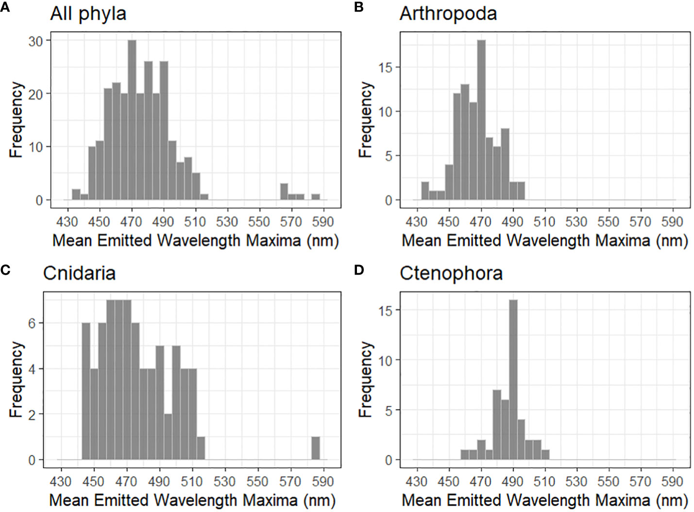
Figure 3 Distribution of mean emitted wavelength maxima for (A) all planktonic phyla with reported mechanically stimulated bioluminescence (n = 247), (B) Arthropoda (n = 87), (C) Cnidaria (n = 73), and (D) Ctenophora (n = 43). The highest intensity wavelength was used when a species showed multi-modal spectral maxima. All bins are 5 nm.

Table 3

Table 3 Flash kinetics of mechanically stimulated bioluminescent zooplankton and dinoflagellate species.

2.5 Ctenophora

The vast majority of planktonic ctenophores have the ability to bioluminesce (Haddock and Case, 1999; Martini and Haddock, 2017). The difficulty of identifying some species and mistaking a cydippid larva for an adult has sometimes attributed bioluminescent capabilities to non-bioluminescent ctenophores, i.e., the genus Pleurobrachia (Haddock and Case, 1995). Bioluminescence has been reported in five of the seven orders of ctenophores, i.e., Beroida, Cestida, Cydippida, Lobata, and Thalassocalycida (Herring, 1987; Haddock and Case, 1999; Brusca et al., 2016). For M. leidyi, emissions can occur as soon as they are released as gametes from the adults. Bioluminescence occurs along a line of cells within the eight divisions and meridional canals of the ctenophore. On the molecular level, the photons that excite the photosensitive opsins are halted when in the dark and allow for the calcium-regulated luciferin-luciferase reaction to take place (Anctil and Shimomura, 1984). Haddock and Case (1999) reported emission maxima peaking on average at 486 nm and ranging from 458 to 501 nm for the 41 sampled species, with no statistical difference between different orders. Their bioluminescence response can be provoked via mechanical, electrical, and chemical stimulation. Nikolaevich and Vladimirovna (2016) showed they are brightest when they are about to reproduce. Mnemiopsis leidyi and Ocyropsis maculata immaculata have bioluminescent abilities that are photoinhibited by light, making the energetically expensive action of bioluminescence only happen in dark environments when it can be seen (Haddock and Case, 1999). As with several other clades, bioluminescence is most likely emitted by ctenophores to startle potential predators.

Because of their high abundance in shallow and coastal waters, several studies have assessed the drivers of ctenophore bioluminescence. Results showed the bioluminescence capacities of these organisms to be highly varied based on abiotic factors and intrinsic characteristics of the individual. Light emitted by M. leidyi and Beroe ovata, for example, can vary based on their diet (Mashukova and Tokarev, 2013), their developmental stage and size (Tokarev et al., 2012), the metabolism of the individual, environmental parameters such as temperature (Nikolaevich and Vladimirovna, 2016), and whether or not they are in the process of regeneration (Mashukova and Tokarev, 2016). It is not known if those parameters affect the flash kinetics of other phyla in the same manner, warranting further research.

The flash kinetics of ctenophores are relatively well studied, and vary with the strength and duration of mechanical stimulation. Widder (1991) measured PI, FF-MSL, RT, and FD for several species; when mechanically stimulated in an integrating sphere, ctenophores can reach very high peak intensities, i.e., Beroe cuvata will peak at 3.40×10¹² photons/s/ind, and will flash for a few seconds, similarly to cnidarians (Table 3).

2.6 Chaetognatha

Chaetognaths, or arrow worms, are planktonic carnivores and are up to 15 cm in length (Pechenik, 2006). They use grasping spines near their mouth to capture prey such as copepods and fish larvae. Martini and Haddock (2017) found approximately 10% of the sampled chaetognath individuals are capable of bioluminescence. Bioluminescent species were found at depths varying from 500 to 3,500 m (Martini et al., 2019). Only two species, Caecosagitta macrocephala and Eukrohnia fowleri, are known to be bioluminescent (Haddock and Case, 1994; Thuesen et al., 2010). Both these species will release clouds of luminous material upon mechanical stimulation, most likely for defense and escape purposes. Like other deep-sea organisms, their gut lining is bright orange, which would hide the subsequent flashes of ingested copepods or other bioluminescent preys (Thuesen et al., 2010; Thuesen and Haddock, 2013). Little is known on their flash kinetics, other than C. macrocephala emissions peaking at 467 nm. The hexagonal shape of the chambers containing the luciferins and luciferases is unique among bioluminescent organisms (Thuesen et al., 2010).

2.7 Chordata

There are two classes of bioluminescent planktonic nonvertebrate chordates: the gelatinous house-building appendicularians (Larvacea) and the thaliaceans (salps, doliolids, and pyrosomes).

Larvaceans are tadpole-like organisms that secrete a mucus house around them several times every day. This house is used for filtering food particles pushed by the current created by the larval-like tail of the organism. The house is then ingested with the captured particles or discarded into the water column (Brusca et al., 2016). Owing to their rapid growth rates and the quick turnover of the house, recent studies have shown that the contribution of larvaceans to the carbon pump has been underestimated, further increasing the importance of gelatinous plankton in marine pelagic ecosystems (Jaspers et al., 2023). Unlike other groups of chordates, MSB is widespread in appendicularians. Both the individuals and the secreted houses can bioluminesce when mechanically stimulated (Widder et al., 1989). Galt (1978) observed houses can bioluminesce up to 4 h after being discarded, although captured particles like dinoflagellates can also bioluminesce, thus making accurate measurements of their bioluminescence quite variable and complex (Galt and Sykes, 1983). The mechanically stimulated bioluminescence of the Oikopleura genus has been measured and studied using a bathyphotometer pumping at 15 L/min, with peak emissions of 1.7×10¹¹ photons/s at 483 nm (Widder et al., 1983; Swift et al., 1985). An interesting observation by Galt and Sykes (1983) is that the kinetics of the organism itself and its house are very different from each other, i.e., the RT of the organism is about half of the house’s (see Galt et al. (1985) for a detailed list of larvacean flash kinetics). In these experiments, larvaceans and their houses were mechanically stimulated by injecting a volume of seawater into the sample vial, creating flow within. At least in Oikopleura rufescens, Megalocercus huxleyi, and two species of Vexillaria sp., light is produced in micrometer-sized granules located on the house rudiment and the secreted house (Galt et al., 1985). Both Martini and Haddock (2017) and Galt et al. (1985) agree appendicularians species, when present, are usually bioluminescent and occupy a significant proportion of the water column’s planktonic biomass. Alldredge (1972) measured densities of discarded houses of Oikopleura spp. at up to 623 houses/m³. Considering the enormous planktonic biomass these houses represent, coupled with their bioluminescence capabilities, these gelatinous structures could contribute a significant fraction of extrinsic MSB for upper trophic levels (Gorsky and Fenaux, 1998; Purcell et al., 2005). Most of the species of larvaceans with described flash kinetics are from the Oikopleura genus, although most appendicularians are known to be bioluminescent.

Salps are mainly colonial and can form chains of organisms several meters in length. Doliolids are small solitary organisms, i.e., less than 1 cm, but some species can be seen forming planktonic colonies (Brusca et al., 2016). Most of the described species of salps and doliolids are not bioluminescent. Little is known on the bioluminescence across these two groups, and even less on their flash kinetics and the function of their bioluminescence. However, one would expect development in this field with recent advances in deep sea in situ measurements and gelatinous plankton sampling methods (Robison et al., 2005).

Pyrosomes are cylindrical colonies made of millimeter-sized individuals found in every ocean, in the top layers of the water column (De Carvalho and Bonecker, 2008). Pyrosomes can be significant contributors to carbon export and can rapidly form blooms, changing water column diversity and bioluminescence profiles (Lilly et al., 2023). The bioluminescence of the Pyrosoma genus has been well documented. Their bioluminescence is interesting in the sense that flash duration is extremely long, i.e., up to 1 min. The response can also be provoked by mechanical, photic, and electrical stimulation. Bowlby et al. (1990) and Nicol (1958a) estimated the FF-MSL of Pyrosoma atlanticum to be up to 2.30×10¹³ photons/ind through mechanical stimulation in an integrating sphere, possibly due to the significant size of the colony. The spectral properties of this species are unique due to a bimodal spectrum with a main and secondary peak at 493 and 471 nm, respectively (Latz et al., 1988). The emission spectra of P. spinosum was measured at 485 nm (Swift et al., 1977). However, pyrosomes being colonial species, the number of individuals and the total area of the colony are highly variable, thus introducing variance in the BP-MSL of the species (Bowlby et al., 1990). In P. atlanticum, bioluminescence is caused by the microbial symbiont Photobacterium Pa-1 (Berger et al., 2021). Further studies are needed to assess the bioluminescence mechanisms of other pyrosomes. Bowlby et al. (1990) noted mechanical stimulation produced the strongest bioluminescence with a flash duration of 59 s on average. Their mean RT is also one the longest observed with 20 s before reaching maximum intensity. With such flash kinetics, pyrosomes have one of the longest MSL flashes ever described among marine plankton.

2.8 Radiolaria

Radiolarians are small protists, with both solitary and colonial species, that are exclusively marine, planktonic, and can have an internal siliceous skeleton (Brusca et al., 2016). They are mostly found in tropical, warmer waters. MSL has been confirmed in at least six taxa (Latz et al., 1987b). Bioluminescence in radiolarians most likely serves as a predator deterrent, similar to dinoflagellate species (Herring, 1979). Latz et al. (1987b) identified radiolarians as important contributors to surface bioluminescence in the Sargasso Sea. However, their small size and difficulties associated with collecting and preserving these species might contribute to underestimating their contribution to planktonic MSL. In colonial species like Acrosphaera murrayana, Siphonosphaera tenera, or Collosphaera spp., bioluminescence is emitted from multiple points within the colony. Radiolarians have long flash durations varying from 1 to 5 s (Latz et al., 1987b; Latz et al., 1991), which is much longer than most other planktonic bioluminescent species and other unicellular organisms, i.e., dinoflagellates (Table 3). Measured PIs are within the lowest order of magnitude observed for dinoflagellates, with 6.70×10⁸ photons/s for Thalassicolla nucleata (Latz et al., 1991).

2.9 Summarizing diversity of MSB emission spectra and flash kinetics

Published mean emitted wavelength maxima are compiled for each phyla with described planktonic bioluminescent emissions (Table 2, Figure 4). These maxima are 528.9 ± 41.0 nm for annelids, 467.0± 12.5 nm for arthropods, 467.0 nm for chaetognaths, 488.7 ± 9.80 nm for chordates, 470.4 ± 55.7 nm for cnidarians, 486.9 ± 10.1 nm for ctenophores, 476.6 ± 3.20 nm for dinoflagellates, and 450 ± 5.00 nm for radiolarians (Figure 4). Only one of the two bioluminescent species of chaetognath has its spectral properties described (Thuesen et al., 2010). Owing to several species—mainly from the genus Tomopteris—producing yellow bioluminescence, the phylum Annelida has the highest mean emitted wavelength maxima of all compiled phyla. The bandwidths at which emissions reach half of the maxima’s intensity (FWHM) are also listed for several species in Table 2. These FWHM are typically broadly ranging from 50 to 100 nm except for the dinoflagellates, where this bandwidth ranges from 35 to 38 nm for the four species with available data.

Figure 4

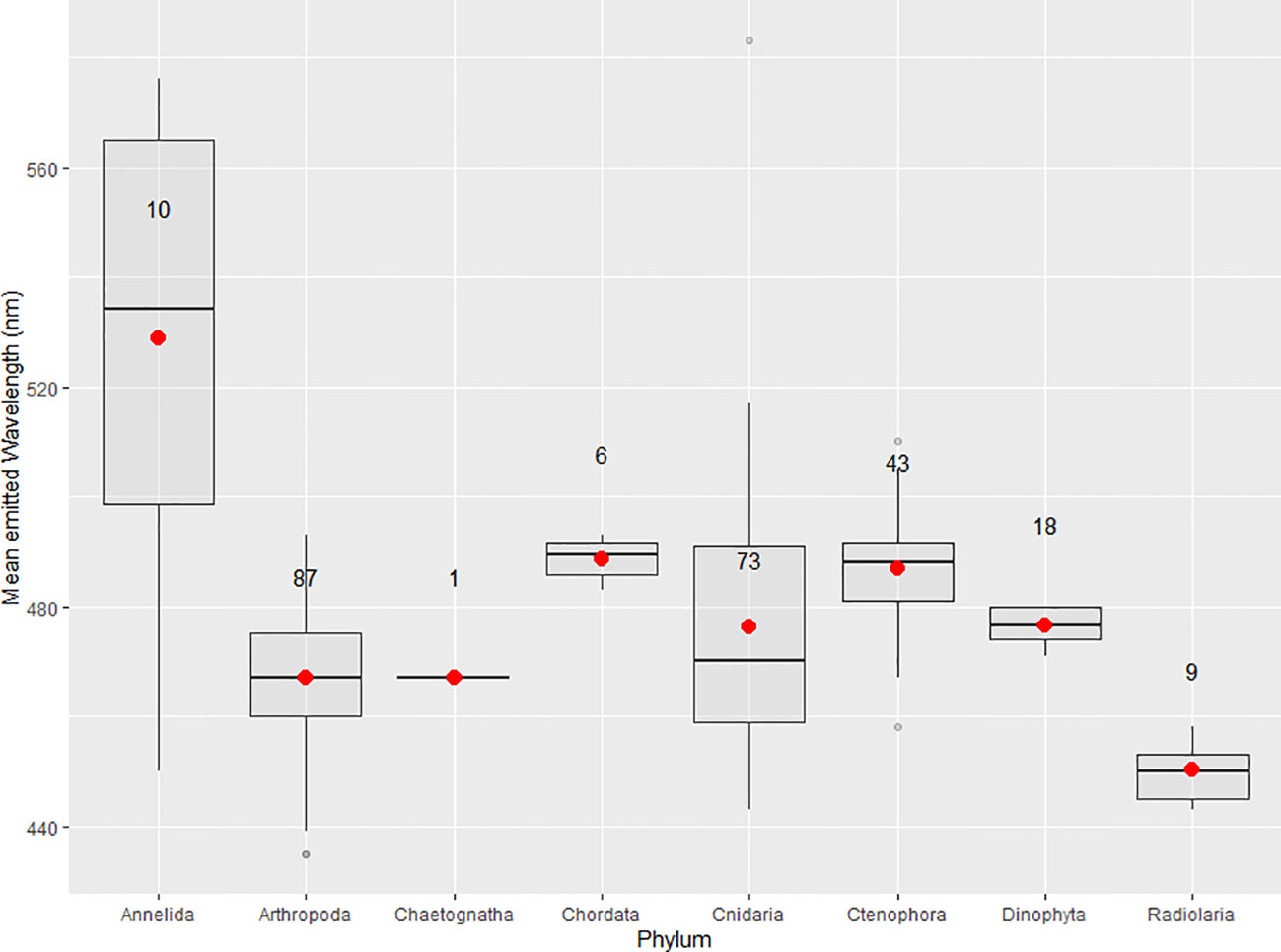
Figure 4 Boxplots of the mean emitted wavelength maxima for phyla with described bioluminescent planktonic species. Red dots indicate the mean of the distribution and sample size is displayed on every boxplot. Maximal wavelengths 2 standard deviations above or below the phyla's mean are displayed as outliers.

Haddock and Case (1999) have found for gelatinous plankton, i.e. ctenophores, cnidarians, and non-vertebrate chordates, wavelength maxima can be correlated to the depth at which the species are found, with deeper species having maxima that are increasingly blue-shifted (Reynolds and Lutz, 2001). This presumably is due to deeper waters having peak transmissions increasingly blue-shifted with increasing water clarity, likely an adaptation to optimize signaling. Matching peak emission with peak transmission through water has a lower energetic cost per emission than other wavelengths, assuming the photon flux is identical. This would also explain why most phyla have their mean emitted wavelength maxima for clear ocean water in the 450–500 nm range (Table 2), and why phyla with wider water column distributions such as cnidarians have broader wavelength ranges than organisms such as dinoflagellates. Bioluminescence spectra also vary based on habitat. Coastal species will tend to have emission maxima between 490 and 520 nm, whereas maxima of clear open ocean species are often between 450 and 490 nm, most likely due to higher turbidity and dissolved organic matter in coastal waters (Hastings, 1996). These ranges include benthic and sessile species, in addition to planktonic and nektonic organisms, presumably because all of these species are using bioluminescence to signal through the water column.

Out of all the phyla compiled, cnidarians show the largest range in mean emitted wavelength (Figure 3). This is because most species of cnidarians emit in the green-blue range, although Erenna sirena has distinctive red bioluminescent lures. Relatively high absorption by water in the red would suggest that these emissions have evolved to be impactful over relatively small distances. The distribution among cnidarians does not follow a normal distribution curve of mean emitted wavelength maxima (Figure 3). This might be because cnidarians are found in almost every marine system and throughout the water column. This allows for very different water clarity conditions, water composition, and prey–predator relations, which can all be evolutionary drivers for spectral bioluminescent emissions.

Figure 3A shows the distribution of mean emitted wavelength maxima for all species from Table 2; Figures 3B–D show the three phyla with most described species that have mechanically stimulated bioluminescence (Arthropoda, Cnidaria, and Ctenophora). The mean emitted wavelength maxima distribution for dinoflagellate species is not shown in Figure 3 since its low sample size did not allow for a representative histogram. Shapiro–Wilk tests were made for all wavelength data and for phyla in Figure 3. p-values for the Arthropoda and Ctenophora distributions were 0.246 and 0.193, respectively, thus accepting the hypothesis of normal distribution at a significance level of 5%. This was not the case for the phylum Cnidaria and for all wavelength data combined. A non-parametric one-way ANOVA was applied to identify any significant differences in wavelength maxima distributions. Following an ad hoc Dunn test, it was identified that Arthropoda’s distribution is statistically different from the phyla Annelida, Chordata, Cnidaria, and Ctenophora (p < 0.05). The differences in distributions for Ctenophora and Cnidaria, in addition to Annelida and Cnidaria, were also significant. All other comparisons of phyla were inconclusive.

Since arthropods, cnidarians, and ctenophores all use coelenterazine for bioluminescent emissions, it is interesting that their spectral properties are all statistically different (Haddock et al., 2010; Widder, 2010a). However, the small sample sizes for annelids, chordates, and dinoflagellates may not allow for accurate representation of the phyla and sufficient statistical outputs.

Considering the dominance of bioluminescent traits across zooplankton clades and the number of known bioluminescent species, only a handful have had their emissions measured quantitatively, and even less have had their flash kinetics described (Haddock et al., 2010). For example, Herring (1988) lists 58 species of confirmed bioluminescent copepods, with an additional 26 with unconfirmed bioluminescence (i.e., misidentified species, anecdotal observations, and observations from non-monospecific cultures), while only 12 species have partially described flash kinetics (Table 3). Similarly, Marcinko et al. (2013b) lists 68 species of dinoflagellates with confirmed bioluminescence, while the only metric that is widely available is total mechanically stimulated light for most measured species. The genera Gonyaulax and Protoperidinium have the best coverage for TMSL data, but other dinoflagellate clades have poor taxonomic coverage.

3 Measuring mechanically stimulated bioluminescence

A wide variety of methods have been used in controlled laboratory environments for applying shear in MSL measurements, including Couette flow, pipe flow, microfluidic constriction, microfluidic obstruction, Svet, orbital shaker, various stirring apparatuses, acoustic pressure, applying a vacuum, and using a needle probe. The Svet is a photometer system using water flow to stimulate bioluminescence within a cuvette, differing in sizes based on the organisms being tested (Tokarev et al., 2012; Mashukova et al., 2016; Nikolaevich and Vladimirovna, 2016). Light is collected via a photomultiplier tube (PMT) that sits 1 cm away from the cuvette (Mashukova et al., 2023). Samples are maintained in constant stimulation in view of this PMT until the bioluminescent response has ended. The magnitude and duration of shear stress applied is often not considered, however. Since emission intensity and other kinetic parameters are usually dependent on the magnitude of shear stress imposed by a given approach (Latz and Rohr, 2013), interpreting and comparing results can be difficult. Some aspects of emission such as flash duration and the rate of decay from peak emission, i.e., e-folding, are less dependent on the intensity of incident shear and, thus, are more comparable between techniques and organisms. Important exceptions in using quantifiable shear in experimental work are the simple Couette flow and pipe flow approaches (Rohr et al., 1999; Latz et al., 2004a; Jing et al., 2011), where repeatable, well-characterized fluid shear stress levels can be used to characterize MSB dynamics.

Measuring bioluminescence in situ is a challenging problem from both engineering and biological perspectives. Bioluminescence occurs throughout all ocean depths and organisms can be patchy and elusive with various sampling approaches. From micron-sized bacteria to colonial gelatinous plankton reaching meters in length, PIs of flashes span at least nine orders of magnitude (Widder, 2010a) and resolving full kinetics requires sensitive low-light detector(s). With kinetic parameters being dependent on incident shear levels, an understanding of the associated small-scale fluid dynamics for a given approach can be vital in interpretation. In fact, to fully describe and interpret MSL, one must also understand the effect abiotic and biotic factors can have on the bioluminescent manifestations of an organism, including recent history of exposure to light and other potential sources of shear (Valiadi and Iglesias-Rodriguez, 2013). Moreover, every measurement approach has advantages and disadvantages and assumptions in interpretation must practically be made. Furthermore, no one approach will work for all organisms.

Discussed below are three general approaches in measuring bioluminescence in situ: (1) the flow-through bathyphotometer, (2) imaging a mesh net, and (3) passive detection.

3.1 Flow-through bathyphotometers

Bathyphotomers use flow agitation within an enclosed chamber to mechanically stimulate bioluminescence (Herren et al., 2005; Latz and Rohr, 2013). The Seliger bathyphotometer from 1968 was the first system measuring bioluminescence to quantify the abundance of source organisms (Seliger and McElroy, 1968). This bathyphotometer was equipped with an impeller facing a PMT, ensuring water flow would be directed toward the PMT and emissions would be captured. In the next iteration of this bathyphotometer, mechanical stimulation of organisms was achieved through flow constriction into a 1.5-inch-diameter hole facing the PMT. It was used in the bioluminescent bays of Jamaica and Puerto Rico to measure the abundance of the dinoflagellate Pyrodinium bahamense (Seliger and McElroy, 1968; Seliger et al., 1969), contributing to an understanding of the mechanisms that contributed to their high abundance in the bays (Seliger et al., 1971).

The most commonly implemented approach for measuring MSL in situ has been the mixing chamber bathyphotometer, which is also the design employed for the only commercial off-the-shelf embodiment, the Underwater Bioluminescence Assessment Tool (UBAT; Seabird Scientific, www.seabird.com, Bellevue, WA). These sensors have relatively slow flow rates, typically ranging from 0.2 to 1 L/min, and a single, small mixing chamber, and thus can be compact and practical in deployment. Besides UBAT, examples of past iterations of this design include the MBBP models from Dr. Jim Case’s laboratory at UCSB (Herren et al., 2005) that served as predecessors of the UBAT, a bathyphotometer developed at URI in the 1980s (Swift et al., 1985), the Over-The-Side (OTiS) bathyphotometer (Bivens et al., 2001), NOSC (Latz and Rohr, 2013), and BIOLITE (Latz and Rohr, 2013). Organisms are mechanically stimulated before the flow enters the mixing chamber using means including an impeller pump, flow constriction, or flow obstruction. A sensitive detector such as a PMT is positioned in close proximity to the mixing chamber. Advantages of this approach include compact size and ease of deployment. The 60-Hz sampling rate of the UBAT is capable of resolving flash kinetics for individual organisms. This makes the identification of source organisms possible based on their flash properties (Johnsen et al., 2014; Cronin et al., 2016; Messié et al., 2019; Chen et al., 2023).

Both the URI bathyphotometer and the NOSC used a pump downstream, creating turbulence in the mixing chamber to mechanically stimulate organisms (Latz and Rohr, 2013). Measurements by the URI bathyphotometer, as well as those by the NOSC bathyphotometer, were coupled with abundance data obtained from net tows to calculate light budgets that determined the contribution of source organisms to the bioluminescence field (Swift et al., 1983; Lapota et al., 1989; Lapota et al., 1992a; Lapota et al., 1992b; Swift et al., 1995).

The only other commercialized bathyphotometer is the GlowTracka (Chelsea Technologies, UK), a small low power, low flow rate instrument that uses a photodiode as a light detector. Despite limited sensitivity, it is still suitable for coastal areas with high levels of dinoflagellate bioluminescence (Kim et al., 2006; Le Tortorec et al., 2014; Parvathi et al., 2021).

Drawbacks of mixing chamber bathyphotometers such as UBAT include (1) poorly defined levels of shear in most iterations, (2) low flow rates creating a likely severe underrepresentation bias for mobile zooplankton able to avoid entrainment, and (3) potential prestimulation in entrance tube configurations transporting the water to the agitator. There is also the inherent property of a mixing chamber being fully turbulent, resulting in ambiguity in (1) the number of secondary stimulations occurring within the chamber, and (2) the residence time of an organism in the chamber, ultimately defined by a probability distribution function. Consequently, measured MSL in photons/L from different mixing chamber bathyphotometers are not directly comparable but may be correlated (Latz and Rohr, 2013), especially considering there are idiosyncratic time dependencies that are not typically characterized.

In the 1990s, the HIgh flow rate Defined EXcitation (HIDEX) bathyphotometer and associated variants were developed (Widder, 1991; Bivens et al., 2001; Widder et al., 2003) to address some of the ambiguities related to mixing chamber bathyphotometers. Organisms were mechanically stimulated as they flowed through a circular grid with a square hole pattern with 1-cm spacing; this form of excitation has readily modeled hydrodynamic and shear stress properties (McKenna and McGillis, 2004; Lacassagne et al., 2020). First flash MSL kinetics were then resolved by an array of PMT detectors lining a 1.6-m tube, removing residence time ambiguity and potential secondary flashes as laminar pipe flow quickly develops after initial grid stimulation (Widder et al., 1993). An integrated measurement of total intensity was also measured via an array of optical fibers surrounding the tube, all coupled to a single PMT. Flow rates could be varied and were typically kept between 18 and 22 L/s in field measurements. This relatively rapid flow rate was essential when trying to entrain mobile zooplankton as small as copepods with the ability to instantaneously leap up to 1 m when threatened, although some behavior avoidance was still likely. Varying flow rate also had the advantage of varying maximal shear rates experienced via grid stimulation. The bathyphotometer tube was opaque and had a helical, rotating baffle upstream of the stimulation grid to minimize ambient light from entering the tube; the baffle shape was designed to minimize prestimulation of organisms. HIDEX instruments were deployed by the US Naval Oceanographic, the Naval Ocean Research and Development Activity (NORDA), the Naval Oceanographic and Atmospheric Laboratory (NOARL), and the Naval Research Laboratory (NRL) until the mid-2000s but were never commercialized for general use.

At a flow rate of 18 L/s, the residence time of an organism traversing the HIDEX bathyphotometer tube was approximately 1 s. All the emission kinetic parameters discussed in Section 2.8 could be resolved. For organisms with flashes longer than 1 s (see Table 3), all kinetic parameters were still generally resolvable except for flash duration, which may still be inferred in typical cases. Zooplankton with minimum length scales greater than 1 cm could not be resolved, and rapid flows impacting a grid can also disintegrate delicate organisms such as some gelatinous plankton, with associated emissions being more consistent with a “death glow” than typical MSL. Durations of death glows of gelatinous plankton are typically much longer than natural MSL, often lasting tens of seconds (Bowlby et al., 1990; Widder, 1991). Despite these drawbacks, to which we can add the HIDEX system was about the size of a small car and challenging to deploy, measurements of MSL with HIDEX may be considered the most precise ever made in situ.

Bathyphotometers have been profiled from a ship, towed by a ship, deployed as an expendable probe (Case et al., 1993; Fucile et al., 1999), configured in flow-through mode on a ship (Bivens et al., 2002; Latz and Rohr, 2013), autonomously moored (Berge et al., 2012), and mounted on AUVs (Thomas et al., 2003; Moline et al., 2009; Johnsen et al., 2014) mounted on a Slocum glider (Shulman et al., 2020). Any particular deployment approach may have advantages based on a specific research application.

3.2 In situ stimulation by a mesh grid

Another in situ MSB approach is imaging a mesh grid producing mechanical contact of fluid shear by moving through water, either by vertical profiling from a ship (Priede et al., 2006; Craig et al., 2009; Craig et al., 2010) or by horizontal transects from a moving submersible (Widder et al., 1989; Widder, 2002; Malkiel et al., 2006). Termed the Spatial PLankton Analysis Technique CAMera (SPLATCAM), a low-light camera (ISIT in this case) is focused on a mesh grid approximately 1 m away (Widder and Johnsen, 2000). Shear stress is produced as the grid moves through the water and flashes from dinoflagellates, copepods, euphausiids, and gelatinous organisms were differentiable. When capturing bioluminescent emissions with a single camera, there is a trade-off between imaging the organism, which requires illumination, and seeing the bioluminescence under low-light conditions. To counter this problem, Widder (1992) developed a dual camera system, where an infrared camera captured the organism and an ISIT camera captured the emission. Since the two cameras capture in different spectral regions, the organism and its emissions can be distinguished at the same time. This can be a valuable tool when studying small-scale interactions like predatory events involving dinoflagellates and fast swimming copepods, i.e., displays of the burglar alarm hypothesis.

3.3 Passive detection

With passive detection approaches, stimulation occurs naturally from biological activity and from physical instabilities such as breaking of surface and internal waves (Stokes et al., 2004), boundary layer currents, bubbles (Deane et al., 2016), swimming dolphins (Rohr et al., 1998), deep-sea infrastructures (Tamburini et al., 2013; Holzapfel et al., 2023), etc. Emissions are resolved with a sensitive detector or imaging system (Roithmayr, 1970; Nealson et al., 1984; Buskey and Swift, 1990). With this approach, the relative placement of a detector can significantly impact bioluminescence estimates. Nealson et al. (1984) measured 10 to 25 times more bioluminescence when a passive detector was positioned over the side of a boat looking down in the water column compared to another passive detector moored at 40 m looking up through the same water column. Presumably, there were more bioluminescent organisms and more shear in surface waters from higher biological activity and potentially from physical instabilities. However, attenuation of emitted light through the water column will have a significant but unknown impact on passive measurements, as the distances of individual emissions to the detector and the optical properties of the water are ostensibly unknowns. For example, passive emissions in the Nealson et al. study could have been similar throughout the water column but water clarity could have been poorer near 40 m than near the surface. While detection of naturally induced bioluminescence may thus be difficult to interpret, it can still be important for assessing impacts on ambient light fields, which is the property being directly measured (Craig et al., 2011). Tamburini et al. (2013) observed mechanically stimulated bioluminescence at the ANTARES neutrino telescope in the deep Mediterranean Sea using low-light cameras. Deep currents passing next to moored infrastructure would create shear stress and bioluminescence events. Temporal kinetic patterns in passive detection may also be valuable in assessing what organisms are present. While intensity of emissions would be difficult to interpret due to unknown attenuation as light propagates to the detector, aspects such as flash patterns, flash durations, rise times, e-folding times, and spectral quality of flashes are all aspects that may have potential diagnostic value if the emissions are sufficiently proximal to the detector. Spatial distributions through remote imaging instead of only using a single sensitive light detector could also be valuable in interpretation, as emissions from colonies, or exuded clouds, secreted extracellular structures, or autotomized limbs could be diagnostic of the specific emitting organism(s). Such imagery may be particularly useful for zooplankton that are too large for an MSL measurement with a particular bathyphotometer and/or for zooplankton able to avoid entrainment in the flow of such sensors. Patterns of emission in imagery may also be used to identify the natural source of shear, e.g., a swimming organism or breaking wave. For emissions imaged from above water (Roithmayr, 1970; Altinağaç et al., 2010), special considerations should be made for filtering of emissions as the light propagates through the water column, which can spectrally shift the peak in radiance (Moline et al., 2007).

4 Distributions of bioluminescent organisms

Zooplankton and dinoflagellates account for almost the totality of the bioluminescence observed at the oceanic’s surface waters (Swift et al., 1983). However, the relative importance of both groups to the water column’s MSL is highly variable. Indeed, Swift et al. (1983) reported the majority of bioluminescence in the Sargasso Sea can be attributed to zooplankton. Batchelder and Swift (1989) provide a comprehensive description of bioluminescent zooplankton of that region, while also providing relative contributions to MSL of the water column. However, the mesh size of their plankton net did not allow for representative sampling of dinoflagellate species. This study was one of the first efforts to develop a light budget for primary bioluminescent groups.

In many cases, zooplankton are not the main contributor to water column bioluminescence. Lapota et al. (1989) estimated the bioluminescence of zooplankton in the first 100 m of Vestfjord, Norway was approximately 4% of the total bioluminescence measured, although bioluminescent zooplankton biomass was also low during the sampling period. With these differences in mind, it is clear that a multitude of variables can affect the bioluminescence of a given system, e.g., timing, location, primary production, diversity, and community composition (Neilson et al., 1995; Craig et al., 2010; Haddock et al., 2010; Wimalasiri et al., 2020). For example, recent increases in temperature in Antarctic waters have changed the planktonic community from dominant krill swarms to salp colonies, reducing the bioluminescence of the water column by half (Melnik et al., 2021). The depth of maximum bioluminescence also varies throughout the day, following the diel vertical migration of zooplankton (Berge et al., 2012; Shulman et al., 2012), although some studies attribute the diel variation of bioluminescence mainly to the circadian photoinhibition of dinoflagellates and select zooplankton (Batchelder et al., 1992; Mashukova, 2009). Lapota et al. (1992a) observed a significant difference in the contribution to total bioluminescence of dinoflagellates and zooplankton, depending on if they were sampling under the sea–ice interface or in the marginal ice zone (MIZ). In the first 10 m of the MIZ, the dinoflagellates Protoperidinium spp. represented 90% of total bioluminescence, whereas in the open ocean, that same percentage was attributed to the copepod Metridia longa. Although Buskey (1992) did not observe significant differences in the epipelagic bioluminescence between the MIZ and open waters of the Greenland Sea, the relative contribution of copepods, larvaceans, ostracods, and krill varied considerably over time, and dinoflagellates accounted for a very small percentage. Approximately 60%–80% of species are bioluminescent in the open ocean, compared to 1%–2% in coastal environments (Morin, 1983). However, these very few bioluminescent coastal species often dominate the water column in biomass.

When measuring bioluminescence throughout the water column, peak MSL usually occurs in the mixed layer or near the thermocline (Wimalasiri et al., 2020). Indeed, this is typically a region of higher phytoplankton productivity, on which bioluminescent zooplankton can thrive. The pycnocline is also a relatively discrete region of the water column, often with high shear (Basterretxea et al., 2020). Considering most bioluminescent zooplankton can produce light when mechanically stimulated and that total emission is correlated with shear levels, the pycnocline typically is a region of high MSL (McManus et al., 2003; Polonsky et al., 2020). On a global oceanic scale, bioluminescence in Atlantic surface waters has been linked to coastal upwelling currents, with an easterly decreasing gradient (Piontkovski et al., 1997). Staples (1966) provides an extensive review of bioluminescence events and their seasonal variation in most major oceanic basins. Peaks and variations in bioluminescence have also been linked to internal waves in the tropical Atlantic (Kushnir et al., 1997). High bioluminescence has been measured in thin sound scattering layers in the Gulf of Maine, for which the euphausiid Meganypctiphanes norvegica and the ctenophore Euplokamis sp. were thought to be the main species responsible (Widder et al., 1992). Acoustic instruments able to map patchy zooplankton in the water column on fine scales suggest that previous estimates of zooplankton MSB may be significantly underestimated (Benoit-Bird et al., 2010b; Moline et al., 2010; Sullivan et al., 2010). Indeed, MSL is as much as 200 times greater in thin sound scattering layers than background bioluminescence outside them (Widder et al., 1992). This is further complicated by the vertical migration of these sound scattering layers, effectively moving bioluminescence hot spots through the water column with isolumes (Clarke and Backus, 1964; Clarke, 1971). Ancillary acoustic measurements can therefore provide vital fine-scale spatiotemporal information when trying to study zooplankton bioluminescence, considering the inherent patchiness and their diel vertical migrations sometimes spanning hundreds of meters (Boden, 1970).

Discriminating assemblages of bioluminescent organisms typically requires relatively laborious net tow collections followed by microscopic identification of individual organisms on a ship by a taxonomist. There are, however, submersible microscopic imaging systems that may now be employed to image organisms in situ and quantitatively assess their distributions through automated machine learning algorithms (Sosik and Olson, 2007; Guo et al., 2021; Le et al., 2022). Higher organism counts can usually be obtained using these approaches and the imaging system can be collocated with a bathyphotometer during deployments. Submersible imaging microscopes developed over the last 15 years include (1) holographic imagers such as the custom HOLOCAM and AUTOHOLO developed at Harbor Branch Oceanographic Institute (Florida Atlantic University) (Nayak et al., 2016; Nayak et al., 2019; Barua et al., 2023) and the LISST-HOLO commercialized by Sequoia Scientific (www.sequoiasci.com; Bellevue, WA), (2) designs based on conventional microscope and cytometer approaches like the FlowCytobot (IFCB) (Olson and Sosik, 2007; Orenstein et al., 2020), and (3) shadowgraph imagers such as those commercialized by Bellamare (www.bellamare-us.com; Miami, FL). Since these instruments could be used to image organisms in close proximity to the bathyphotometer, it may be possible to verify organism diversity in separate net and bottle sampling in situ.

5 Applications for studying and measuring bioluminescent emissions

Biological oceanographers can consider light emissions in the water column as a proxy for the abundance and diversity of bioluminescent organisms when studying marine systems. Bioluminescence can also serve as a proxy for biomass (Squire and Krumboltz, 1981), primary and secondary production, remote identification and monitoring (Johnsen et al., 2014), and long-term climate change impacts (Piontkovski and Serikova, 2022). The following section describes applications for measuring bioluminescence and flash kinetics in marine ecosystems.

The patchiness of zooplankton populations in the water column is a subject of interest in remote sensing and acoustics studies (Jaffe, 1999; Holliday et al., 2003; Taylor et al., 2005; Sullivan et al., 2010; Basedow et al., 2019). In systems where zooplankton bioluminescence is dominant, vertical profiles of the BP-MSL can offer insight into the distribution of the zooplankton in the water column (Gitelson and Levin, 1989). In addition to net tows at depth and acoustic profiling, bioluminescence profiles can be an additional tool in these studies trying to resolve zooplankton spatial composition. Cram and Malan (1971) proposed the bioluminescence of krill, a very important functional group to both fisheries and marine ecosystems, may be their best characteristic for remote sensing. In Widder et al. (1999), bioluminescence was used to precisely pinpoint thin layers half a meter thick of high biomass of the copepod Metridia lucens, instead of sampling zooplankton with conventional net methods every meter and potentially missing aggregations.

5.1 Bioluminescence as a tool for flow visualization

Bioluminescence can be used to study biological hydrodynamics, which are often very complex systems to model. Knowing the shear stress threshold to trigger a flash response can provide rapid insight into the state of the system, essentially using dinoflagellates as flow markers (Latz et al., 1995), and offers opportunities to model their flash response (Deane and Stokes, 2005). Bioluminescent flashes of dinoflagellates were studied by Rohr et al. (1998) to resolve the flow around a swimming dolphin. It was concluded that levels of shear stress greater than threshold were achieved over most of the dolphin’s body, except for the head, rostrum, and fins. Bioluminescence emissions were correlated with boundary layer thickness and identified regions where separation of the flow from the body occurred. A similar study was done a decade prior with harbor seals, essentially identifying three zones of high shear through bioluminescent emissions, i.e., whiskers, shoulders, and hind flippers (Williams and Kooyman, 1985). Hobson (1966) suggested this same species might use bioluminescence around swimming prey as a hunting strategy at night. This is of interest to biological oceanographers, functional morphologists, and fluid mechanics experts by providing an unusual approach to identifying high shear zones, quantifying drag around a moving object in water. Researchers studying ocean currents may benefit from dinoflagellate bioluminescence, as Rohr et al. (2002) suggested they be used to identify high-energy zones with prominent stratification.

5.2 Bioluminescence to locate fish populations

Fish schools swimming through the water column will also trigger bioluminescent displays. These emissions can be monitored from boats or aircraft to detect fish populations at night. Squire and Krumboltz (1981) describe such a technique using a low-light video system capturing the bioluminescence created by anchovies triggering planktonic bioluminescence. Other fish species of considerable economic value, i.e., mackerel, sardine, herring, and yellowfin tuna, have also been detected by fishing vessels at night using water column bioluminescence (Roithmayr, 1970). Experienced fishermen can evaluate school biomass based on the size of the bioluminescent cloud and identify fish species based on patterns of bioluminescence propagation (Altinağaç et al., 2010). On the other hand, it has been suggested that water column bioluminescence created by fishing nets may trigger either avoidance or attraction behavior by fish (Jamieson et al., 2006). Monitoring bioluminescence above the water surface could prove a useful technique and asset for fish school sighting and biomass estimation by fisheries and population monitoring programs.

5.3 Correlation of bioluminescence with ocean parameters

The same can be said for the planktonic biomass itself. Considering that a considerable fraction of zooplankton species have bioluminescent capabilities, one can use bioluminescence measurements to infer the primary and secondary production of the water column (Craig et al., 2010). Other variables also covary with water column bioluminescence. In the Mediterranean Sea, surface chlorophyll a correlated with MSL and could be used to predict bioluminescent zooplankton abundance in the mesopelagic zone (Craig et al., 2010). Lapota et al. (1989) observed that the same approach could be used to approximate dinoflagellate abundance in a Norwegian fjord. Ondercin et al. (1995) developed a model of North Atlantic water column bioluminescence based on bio-optical properties such as temperature, chlorophyll a, irradiance, mixed layer depth, and nitrate concentration. To understand the variability of bioluminescence in the context of ecology and hydrology, it is important to measure other abiotic parameters simultaneously, such as dissolved oxygen, turbidity, and temperature using instruments such as a CTD/rosette or multiparameter sondes simultaneously (Bivens et al., 2002).

5.4 Identifying luminescent organisms based on flash characteristics

One of the most promising applications for MSB is identifying the presence of specific species without needing to collect organisms (Cronin et al., 2016; Messié et al., 2019). Indeed, since many species have different first flash kinetics, it may often be possible to discriminate between different bioluminescent planktonic clades in situ using a bathyphotometer providing well-resolved levels of shear stress stimulation. This type of autonomous sampling can be of great help in detecting fragile organisms like gelatinous plankton, species living at great depths that would otherwise not be present in net tows, species with very low abundance that would most likely not be sampled over a discrete time period and organisms difficult to culture and maintain in laboratory conditions such as heterotrophic dinoflagellates, larvaceans, and salps. Not only could bathyphotometers detect the presence of specific species with flash kinetics, but the biomass could also be estimated if the integrated bioluminescence of an individual flash is known. Using relative bioluminescent intensities over two wavelengths and first flash kinetics, Nealson et al. (1986) were able to correctly identify 10 species of dinoflagellates, krill, copepods, and corals, with 100% accuracy for some species. More recently, a similar experiment took place in the Arctic where Johnsen et al. (2014) described the variation of bioluminescence over a diurnal cycle and partitioned the total bioluminescence over key clades using the spectral properties and kinetics of bioluminescent flashes. Certain clades can also be identified from images of the bioluminescent flashes. Kocak et al. (1999) developed a model capable of tracking and identifying organisms based on flash size and duration. Bioluminescent emissions observed with the SPLAT CAM have been used to calculate nearest-neighbor distances for dinoflagellate and copepod layers in the Gulf of Maine (Widder and Johnsen, 2000), and to identify thin layers and aggregations of copepods, euphausiids, dinoflagellates, and ctenophores (Widder et al., 1999). Once a species has had its first flash kinetics and spectral properties described, a bathyphotometer could supplement the time-intensive processes of zooplankton fixation and identification in future sampling efforts by providing presence/absence information on finer scales over a much larger area. Messié et al. (2019) used bioluminescence measurements to identify dominant species of dinoflagellates and zooplankton in Monterey Bay, California. Background bioluminescence was associated with dinoflagellates and peaks were assumed to be caused by zooplankton flashes. The simultaneous use of a fluorometer allowed distinction between auto and heterotrophic dinoflagellate species. Based on glider observations of bioluminescence, fluorescence, and optical backscattering, Shulman et al. (2020) demonstrated a shift from an autotrophic and mixotrophic bioluminescent community toward a more heterotrophic one in the Delaware Bay area, DE.

5.5 Bioluminescence assays for toxicology

Bioluminescence measurements using MSL can be useful as sensitive non-lethal proxies for toxic compounds, complementing expensive and time intensive bioassays (Lapota et al., 2007; Widder and Falls, 2013; Perin et al., 2022). Half of the known dinoflagellate clades with bioluminescent capabilities are toxic (Haddock et al., 2010). The proposed method could augment expensive and time-intensive bioassays. Not only could bioluminescence help assess the presence of dinoflagellate toxins in water, but it can also be used to detect blooms at their inception, which is not possible with most alternative methods (Haddock et al., 2010; Le Tortorec et al., 2014; Le Tortorec 2017). Dinoflagellates can bloom rapidly and create health hazards to humans and marine life in coastal environments. Constant sampling and cell counting to monitor populations can be labor intensive. An autonomous underwater bathyphotometer providing real-time in situ BP-MSL of an area prone to harmful algal blooms could detect increases in dinoflagellate populations without the need for constant sampling (Kim et al., 2006). Species like P. bahamense, L. polyedra, and A. monilatum are all bioluminescent and are often responsible for HABs events in coastal Florida or California. Bioluminescence monitoring could also be applied to other invasive species prone to rapid blooming, like the ctenophore M. leidyi in the Black and Caspian Sea (Kideys, 2002). This species is a threat to local fisheries as it decimates zooplankton and ichthyoplankton populations. Melnik et al. (2020) noted that an increase in M. leidyi biomass resulted in a decrease of dinoflagellate bioluminescence in the Black Sea. Since emissions of these two groups are distinct (Table 3), the relative contribution of both to water column bioluminescence may be a good indicator of the ecosystem’s state, and could be measured remotely without intensive field deployments (Widder, 2010b). This could include ballast water monitoring. With over 90% of planktonic cnidarians potentially having bioluminescent capabilities (Martini and Haddock, 2017), their bioluminescence could be monitored to detect gelatinous blooms in the early stages.

5.6 Climate change and bioluminescence

Climate change and ocean acidification are causing rapid changes and shifts in marine communities worldwide (Doney et al., 2012; Beaugrand et al., 2014; Johnsen et al., 2014). Since most marine phyla possess bioluminescent species, climate change is expected to have significant impacts on the MSL of marine systems as well. However, very few studies have looked at the effects of climate change on bioluminescence and oceanic distributions of responsible organisms.

Dinoflagellates of the genus Tripos have many bioluminescent species and have extended their habitable range into warmer waters in the last few decades (Hays et al., 2005). Heating of surface layers in the Gulf of Alaska and Northeast Pacific in 2013 deprived the water column of silica, resulting in a dramatic shift in phytoplankton assemblage from diatoms to dinoflagellates (Arteaga and Rousseaux, 2023). As diatoms are not bioluminescent, a shift to a dinoflagellate-dominated system is expected to significantly increase the bioluminescence of these waters. On the other hand, Hinder et al. (2012) have noted a long-term shift in relative abundance from dinoflagellate to diatoms in the North Sea and Northern Atlantic, which would be expected to result in an overall decrease in coastal bioluminescence.

A particularly important bioluminescent zooplankton group globally is gelatinous plankton, whose blooms are getting larger and more frequent (Siddique et al., 2022). Considering these groups have many bioluminescent species, a concomitant increase in the MSL in diverse oceanic waters may be expected. Brodeur et al. (1999) noted a significant increase in gelatinous plankton biomass in the Bering Sea, mostly from scyphozoan and hydrozoan jellyfish, that was attributed to warming waters. Gelatinous plankton are very tolerant to a wide range of nutrient levels and environmental parameters, and thus can bloom rapidly and cause community changes in surface waters in virtually all of the Earth’s oceans (Condon et al., 2013). Since the mean emitted wavelength maxima of cnidarian species can be statistically distinguished from most other phyla, the spectral properties of bioluminescent emissions could be used to monitor increases in gelatinous biomass and study the effects of climate change on community shifts.

There is now growing evidence that other bioluminescent zooplankton are both migrating in their distributions and shifting in importance in global oceanic ecosystems on time scales relevant for climate change; however, again, our assessment of associated impacts on MSL can only be implied. For example, copepods, main contributors to the ocean’s carbon pump (SampeiH et al., 2009; Pinti et al., 2023), have been found to be migrating hundreds of kilometers northward in the northern hemisphere every decade (Ratnarajah et al., 2023). On the other hand, Edwards et al. (2021) observed a decrease in krill biomass over decade-long observations in the North Atlantic. Euphausia superba, the bioluminescent krill serving as the keystone species of Antarctic food webs with an estimated global biomass of 215 million tons (Cavan et al., 2019), has been found migrating toward the South Pole. Zooplankton body size, which often correlates to bioluminescence intensity (Biggley et al., 1969; Herring, 2007; Tokarev et al., 2012), has been found to decrease with increasing water temperature (Ratnarajah et al., 2023). This will most likely impact the FF-MSL of large bioluminescent organisms, e.g., scyphozoans, siphonophores, ctenophores, and planktonic annelids. Piontkovski and Serikova (2022) noted a significant decrease in the integrated water column MSL of the tropical Atlantic Ocean over a 40-year period, for which zooplankton species are the main contributors, which correlated with increased water temperatures. Another study in Antarctic waters observed a community shift over 20 years, with salp colonies increasing in importance relative to krill with associated bioluminescence decreasing by 50%, which they hypothesized was caused by climate change, specifically warming waters (Melnik et al., 2021). Rigorously testing such hypotheses is difficult, as modeling of zooplankton community composition is a very complex problem requiring robust time series abundance data for all trophic levels on which to base the model (Ratnarajah et al., 2023). A further complication is rapid changes in environmental parameters driven by climate change create conditions that may not be reflected in previous data (Villarino et al., 2015). We note these studies that suggest monitoring zooplankton communities through species-specific flash kinetics in key locations could give valuable insight into species migration and community shifts.

Other effects of climate change have received scarce attention with respect to bioluminescence but likely have significant impacts on the global ocean bioluminescent potential. Global warming is particularly intense in polar regions, which, in turn, will promote the melting of the arctic ice coverage, resulting in increasing global sea level and decreasing seawater salinity [models predict an increase of the sea level between 3.0 and 3.3 mm/year based on current hydrocarbon emissions (Cazenave et al., 2014; Dieng et al., 2017)]. Changes in sea level will change coastal landscapes and are sure to modify their ecosystems and species interactions. Decreasing salinity will select for more generalist-type organisms that can withstand wide environmental ranges. Many such species are bioluminescent, e.g., gelatinous plankton. Additionally, hydrocarbon emissions are responsible for the acidification of our oceans. Models predict acidification of −0.2 pH for the coast of California by 2040 (Marshall et al., 2017). For dinoflagellates, the scintillons, or the cellular organelles responsible for harboring the bioluminescence reaction are activated through a local drop in pH in the cell (Fogel and Hastings, 1972). It is still unclear how environmental changes in the water column’s pH will affect bioluminescent emissions of organisms. With these important and rapid environmental changes in mind, climate change will undoubtedly drive changes in coastal and pelagic bioluminescence through community shifts and changes in the physiology of bioluminescent organisms. Research is needed to better understand how environmental shifts driven by climate change may affect organism bioluminescence kinetics and the role of bioluminescent species in marine systems.

6 Research perspectives, gaps, and biases

Measuring and interpreting bioluminescent emissions and their temporal variation in situ is not a trivial task. In Sections 3 and 5, we discussed the potential challenges and biases one can encounter when measuring the mechanically stimulated bioluminescence of organisms in the laboratory and in situ. Here, we elaborate on research and technology gaps, suggest approaches to standardize measurements, and consider possible broader roles for bioluminescence measurements and first flash characterization in studies of diversity, ecology, functional morphology, and small-scale fluid mechanics.

6.1 Organism emissions

Widder et al. (1999) described a key challenge at the time of publication as the absence of good taxonomic coverage of flash kinetics and spectral properties for most planktonic groups. Unfortunately, few species have had their bioluminescence described since then. As discussed in Section 2.9, it is clear that a minority of the known bioluminescent plankton have described flash kinetics and spectral properties. Studied species also rarely possess a full set of measured kinetics. For example, Widder et al. (1989) observed 30 species of mostly gelatinous plankton with bioluminescent capabilities in the Monterey Canyon. The spectral properties and flash kinetics of some of these species remain undescribed today. Most of the dinoflagellate species with described kinetics are part of the Gonyaulax and Protoperidinium genera (Table 3), while bioluminescence is present in several others, i.e., Alexandrium, Tripos, Pyrodinium, and Pyrocystis (Marcinko et al., 2013b). At least 100 species of ostracods are known, while in 2019, only 31 were described (Cohen and Morin, 2003), and fewer even had their flash kinetics characterized. Though several bioluminescent copepod species have been observed and documented, few have had their bioluminescence response and flash kinetics measured with quantifiable mechanical stimuli (Herring, 1983; Lapota and Losee, 1984; Herring et al., 1993; Widder et al., 1997). In fact, the clades Copepoda, Amphipoda, and Ostracoda, which are all well represented with bioluminescent planktonic species, are identified as among the groups with the most undiscovered species (Appeltans et al., 2012).

There is also a lack of data on intra-specific variations of bioluminescence across different taxa, particularly for zooplankton, and associated drivers for variance in flash kinetics, e.g., ontogeny, size, diet, sex, and life history. For example, larval stages of zooplankton, most importantly crustacean zooplankton, can occupy a large portion of the planktonic biomass; since these larvae often bioluminesce, they may significantly contribute to the MSL in oceanic waters. However, there is scarce data on their kinetics. In the Norwegian Sea, Lapota et al. (1988) found the nauplii stages of the copepod Metridia longa were responsible for 64% of the bioluminescence at 10 m, and 97% at 25 m. Not fully understanding the variation and change of bioluminescence emissions throughout the ontogenies of species that are main contributors to water column biomass can introduce significant bias into the interpretation of results and into planktonic biomass estimations. For example, the copepod Metridia lucens has had its TMSL measured for most of its larval stages and as an adult (Batchelder and Swift, 1989). Mean TMSL varies from 9×10⁹ photons/ind for copepodite stage 2 to 1.08×10¹¹ photons/ind for female adults. Thus, significant variation exists across a developmental gradient and can likely be found in other species of bioluminescent zooplankton that are not direct developers. For the invasive ctenophore Mnemiopsis leidyi, bioluminescence not only varies throughout its development, from 5.00×10⁸ photons/s for eggs to 5.00×10¹⁰ photons/s for adults (Tokarev et al., 2012), but also based on its diet and water column temperature (Mashukova and Tokarev, 2013; Nikolaevich and Vladimirovna, 2016).

Furthermore, very scarce research has been carried out to discern effects of environmental factors such as water temperature, food and nutrients availability, previous light exposure, previous shear exposure, and likely several other variables, on organism emissions. As an example, the FF-MSL of M. longa was not affected by starvation for up to 3 weeks (Buskey and Stearns, 1991). Since baseline flash kinetic response must first be determined for an organism, we are very far from any comprehensive understanding of abiotic factors on emissions.

The circadian timing of an organism and its light and stimulation histories have a strong impact on bioluminescence emissions (Marcinko et al., 2013a). Dinoflagellates are photoinhibited when subjected to light during their scotophase, i.e., nighttime. Sullivan and Swift (1994) measured a decrease in MSL of 90% when Tripos fusus received 1×10¹⁷ m⁻² s⁻¹ of blue light. Photoinhibition has also been measured with the heterotrophic dinofagellate Protoperidinium depressum (Li et al., 1996). Sullivan (2000) observed TMSL of P. noctiluca reached its maximum 2 h into the scotophase, as the scintillons fully migrated to the periphery of the cell. Lapota et al. (1992b) measured the bioluminescence of the dinoflagellates Tripos fusus and Protoperidinium curtipes in laboratory and found light intensities of flashes at night are orders of magnitude higher, even if dark-adapted. To counter this, samples should be grown or kept in reverse day:night light cycles for a few days before measurements are taken (Neilson et al., 1995; Latz and Rohr, 2013). To allow for representative values of flash kinetics, specifically PIs and FF-MSLs, one should avoid any prestimulation of the organism, as subsequent flashes are typically of lesser intensity. A few hours should pass in between measurements with the same organism, allowing for complete dark adaptation and regeneration of luciferin and luciferase. Considering this, one cannot be sure flashes measured in situ are necessarily at full capacity, while laboratory measurements with appropriately rested organisms may be consistently indicative of full capacity flash emissions.

The above leads to an important question, namely, what is the frequency of natural stimulation and emission for an entire assemblage of bioluminescent organisms present in a given environment? Do individuals rarely need to employ a flash to help thwart predation, or on average is this needed once a night, or several times a night? Answers to these questions are ultimately a convolution of a wide range of encounter probabilities both between prey and predators as well as other sources of stimulation such as swimming nekton or a breaking wave. Such naturally occurring emissions must be studied with passive approaches using low-light detectors, which may then potentially aid in interpretation of in situ MSL measurements.

Some groups of gelatinous plankton may also prove to have large inherent variance in their FF-MSL, simply because they form colonies of variable sizes. Siphonophores and salps, for example, are made of hundreds of smaller individuals of different functions, and the total length of the colony can span from centimeters to several meters for the same species, depending on age and potential fragmentation. Evidently, larger colonies will produce more bioluminescence, which can pose problems when describing the bioluminescence of species or creating photon budgets of the water column. Approaches to accurately quantify emission kinetics for such colonies are a significant challenge. In addition, there is evidence that, in some instances, different parts of the colony exhibit very different kinetics (Widder et al., 1989).

When emissions are measured for a species, often only the mean wavelength maxima and peak intensities are measured, which are insufficient to adequately differentiate species in situ due to the intra-specific variation of peak intensity values. This lack of emission data is partly a consequence of the difficulty in culturing some of these species in the laboratory and partly due to the considerable logistics needed to study them in the field. Culturing heterotrophic dinoflagellates or zooplankton requires maintaining several other prey cultures to sustain all the trophic levels needed, which can be very challenging. In the field, sampled species must be collected, maintained onboard the research vessel, dark-adapted, and rested for optimally 24 h, and assessed individually on the ship using a benchtop bathyphotometer capable of fully resolving emission kinetics (Latz and Rohr, 2013). Moreover, this is laborious and resource-intensive. Significant research efforts are clearly needed before we may hope to use flash kinetic signatures to study organism diversity from MSL measurements alone. Establishing a robust library of flash kinetics for zooplankton species would be a powerful addition for in situ identification efforts and biodiversity research. The previously mentioned work of Cronin et al. (2016) and Messié et al. (2019) demonstrate this. Additionally, Davis et al. (2005) used an empirical orthogonal function analysis to not only identify dinoflagellate species, but also isolate individual flashes from mixed data sets acquired with the HIDEX. However, using biologically emitted light as an identification proxy for ecosystem monitoring only becomes useful when the majority of the community has had its kinetics described. With at least 68 bioluminescent dinoflagellate species (Marcinko et al., 2013b) and only two species with complete sets of FFKs (Table 3), additional flash characterization is needed to adequately discriminate species off their bioluminescent emissions. Moreover, considering that between one- and two-thirds of marine species have yet to be described or even discovered (Appeltans et al., 2012), much work is needed to fully describe bioluminescent processes in the marine ecosystems.

6.2 Measurements and distributions

Each type of bathyphotometer is unique in how flow agitation stimulates bioluminescence because of different agitation approaches, residence times, flow rates, and maximal shear stress values, thus typically producing different BP-MSLs for the same population (Latz and Rohr, 2013) and complicating comparisons. There may be linear correlations in BP-MSLs from different devices but the relationships are organism-dependent, so a “transfer function” to convert measurements of any particular natural assemblage from one BP to another is not straightforward, even among BPs using the same approach, e.g., mixing chamber devices. A different flow rate and mode of stimulation will create different velocity gradient environments, i.e., potential for shear stresses, resulting in different observed flash kinetics in a manner specific to each species. Additionally, a higher residency time in a turbulent mixing chamber (dependent on chamber size and flow rate) may allow some species to flash several times, assuming supra-threshold levels of shear stress are maintained. As mentioned, residence times in a mixing chamber are defined by a probability distribution function, so when multiple flashes occur, consistent results and interpretation may only be possible when a statistically significant sample size is achieved for all individual organisms in an assemblage; even for long time series at specific depths, this will not be possible given common distributions of most zooplankton. As a simple example of difficulties in comparison, the HIDEX stimulated 94% of FF-MMSL for Lingulodinium polyedra with a ∼1-s residence time, whereas the UBAT only stimulated 17% while its residence time can be as long as 10 s (Latz and Rohr, 2013). Currently, measurements of MSL and peak intensities should always be referenced to the instrument used.

Considering the above, bathyphotometers with well-characterized, highly constrained shear stress levels are strongly preferred, where all organisms will experience similar maximal shear. For FF-MSL measurements, the sensor should have no secondary stimulation and a residence time long enough to resolve key kinetic parameters. Flow rates should be high enough to entrain small zooplankton. In fact, these were the design criteria leading to development of the HIDEX (Widder et al., 1993). However, even the grid stimulation of the HIDEX with 1-cm grid openings imposes an estimated range in potential maximal shears experienced by an organism of approximately 0.1 to 0.9 Pa at flow rates of 18 L/s depending on their position in the flow, with organisms centered in a grid opening experiencing the least shear (Tanweer et al., unpublished data). While next-generation HIDEX-like sensors are needed, development of new grid designs providing consistent, constrained shear levels for all organisms should be considered.

Since the most important factor introducing variability between different BPs is the shear stress applied, characterization of shear stresses for BPs would seem to create the potential to report MSL in terms of shear stress, e.g., with units of photons s⁻¹ L⁻¹ Pa⁻¹, to help standardize measurements. There are several issues with this, however, the most important being there is a finite range of shears where emissions will be shear-dependent. Each organism has a stimulation threshold below which no emission will occur. Bioluminescence intensity then increases with increasing flow rate and presumably shear stress, until a critical flow rate is achieved, above which there is no further increase in MSL (Widder et al., 1993; Latz and Rohr, 2013). At the very least, the shear stress characteristics of a particular BP should be reported with published MSL measurements to provide some hope the measurements may be repeated in the future. This is also not straightforward, unfortunately, as the shears associated with a sensor must typically be characterized with Computational Fluid Dynamics (CFD) modeling; because there are many input variables in CFD specific to a given configuration, independent validation is highly desirable with approaches such as Particle Imaging Velocimetry (PIV) or shear probes, but this is not always feasible within the flow apparatus of a BP.

There is a lack of long-term time series of bioluminescent measurements, both at the species and ecosystem levels. Without them, bioluminescence studies are a time–space snapshot of a multitude of covarying factors that impact an organism’s or the population’s MSL, including the effects of physical conditions such as winds and tides, seasonal variation, population growth, cyclical change in community assemblage, longer-term climatic variability in assemblages, diel vertical migration of plankton, blooms, impacts of grazing pressure, etc. To our knowledge, the last long-term data of mechanically stimulated bioluminescence was collected in the 1990s and part of the Marine Light Mixed Layers (MLML) and Biowatt projects (Dickey et al., 1986; Marra, 1995; Marcinko et al., 2013b). These studies provided information on long-scale variations of bioluminescence in the North Atlantic over several years caused by community successions, and seasonal changes in environmental variables and optical properties of the water column (Marra, 1995). In an earlier study from the Black Sea over a 12-month period, Bityukov et al. (1967) observed coastal bioluminescence intensity varied by a factor of 4 and was dominated by a population of the dinoflagellate Noctiluca scintillans. The specific drivers for the variation were unknown, however. More recently, a time series on passive MSL of over 10 years was made in the deep Mediterranean Sea (Tamburini et al., 2013; Reeb et al., 2023), where deep-water currents interacting with the infrastructure of the ANTARES neutrino observatory were established as main drivers for bioluminescence.

Not taking into account how the diel space–time variability of organism patchiness contributes to bioluminescent emissions can create an enormous bias in measurements and water column profiles. Indeed, not only does total intensity vary on a temporal scale, but the bioluminescent biomass also travels up and down the water column during diel vertical migration (DMVs) (Batchelder et al., 1992). Not accounting for this migration and sampling at a constant depth could result in misinterpretation of biomass agglomerations and underestimating bioluminescence. To avoid any biases caused by the patchiness of zooplankton, bioluminescence measurements should ideally be made in tandem with high-frequency acoustic mapping to resolve spatial heterogeneity in the water column. Remote acoustic mapping may also be valuable in describing avoidance of in situ instruments by zooplankton (Benoit-Bird et al., 2010a). Additionally, discrete zooplankton sampling must be done with profilers using nets, bottles, etc. to assess species assemblages and densities. Moreover, the study of water column bioluminescence is a complex problem requiring multifaceted and logistically challenging approaches involving several specialized sensor systems.

Haddock et al. (2010) suggest future works on bioluminescence should focus on developing remote and autonomous methods to monitoring bioluminescence in the water column. We build on this statement in proposing that future efforts resolve the intra- and inter-specific variations of bioluminescent emissions and expand our library of bioluminescent signatures to increase the potential and relevance of autonomous monitoring of bioluminescence. Documenting the flash kinetics and spectral properties of bioluminescent species will allow for in situ and remote identification of organisms, which is relevant for monitoring algal blooms, biomass shifts, and ecosystem structure. Developing instruments with high flow rates and defined shear stress levels will provide less variability in measurements and will limit avoidance of zooplankton, allowing for better comparison between studies.

Author contributions

FL: Conceptualization, Data curation, Formal analysis, Investigation, Supervision, Visualization, Writing – original draft, Writing – review & editing. MT: Conceptualization, Funding acquisition, Project administration, Resources, Supervision, Writing – original draft, Writing – review & editing. AB: Writing – original draft. CP: Data curation, Formal analysis, Writing – original draft. ML: Validation, Writing – review & editing.

Funding

The author(s) declare financial support was received for the research, authorship, and/or publication of this article. Funding was provided by a Florida Atlantic University postdoc fellowship grant, by the Indian River Lagoon graduate research fellowship grant from the Harbor Branch Oceanographic Institute foundation, and by the Office of Naval Research (contract N00014-20-C-2035).

Acknowledgments

The authors sincerely thank Dr. James Sullivan from HBOI for his review and comments prior to submission. We are also grateful for helpful and insightful reviews by Edith Widder, Alan Weidemann, and Igor Shulman, and strongly believe they significantly improved this work.

Conflict of interest

The authors declare that the research was conducted in the absence of any commercial or financial relationships that could be construed as a potential conflict of interest.

Publisher’s note

All claims expressed in this article are solely those of the authors and do not necessarily represent those of their affiliated organizations, or those of the publisher, the editors and the reviewers. Any product that may be evaluated in this article, or claim that may be made by its manufacturer, is not guaranteed or endorsed by the publisher.

References

Abe K., Ono T., Yamada K., Yamamura N., Ikuta K. (2000). Multifunctions of the upper lip and a ventral reflecting organ in a bioluminescent ostracod Vargula hilgendorfii (Müller 1890). Hydrobiologia 419, 73–82. doi: 10.1023/A:1003998327116

CrossRef Full Text | Google Scholar

Abrahams M. V., Townsend L. D. (1993). Bioluminescence in dinoflagellates: A test of the burgular alarm hypothesis. Ecology 74, 258–260. doi: 10.2307/1939521

CrossRef Full Text | Google Scholar

Alldredge A. L. (1972). Abandoned larvacean houses: a unique food source in the pelagic environment. Science 177, 885–887. doi: 10.1126/science.177.4052.885

PubMed Abstract | CrossRef Full Text | Google Scholar

Altinağaç U., Özekinci U., Ayaz A., Ozen O., Oeztekin A. (2010). Utilization of a bioluminescent pattern in the encircling gillnet fisheries. Rev. Fisheries Sci. 18, 151–156. doi: 10.1080/10641260903545295

CrossRef Full Text | Google Scholar

Anctil M., Shimomura O. (1984). Mechanism of photoinactivation and re-activation in the bioluminescence system of the ctenophore Mnemiopsis. Biochem. J. 221, 269–272. doi: 10.1042/bj2210269

PubMed Abstract | CrossRef Full Text | Google Scholar

Anderson D. M., Nosenchuck D. M., Reynolds G. T., Walton A. J. (1988). Mechanical stimulation of bioluminescence in the dinoflagellate Gonyaulax polyedra Stein. J. Exp. Mar. Biol. Ecol. 122, 277–288. doi: 10.1016/0022-0981(88)90128-1

CrossRef Full Text | Google Scholar

Angel M. (1968). Bioluminescence in planktonic halocyprid ostracods. J. Mar. Biol. Assoc. United Kingdom 48, 255–257. doi: 10.1017/S0025315400032562

CrossRef Full Text | Google Scholar

Appeltans W., Ahyong S. T., Anderson G., Angel M. V., Artois T., Bailly N., et al. (2012). The magnitude of global marine species diversity. Curr. Biol. 22, 2189–2202. doi: 10.1016/j.cub.2012.09.036

PubMed Abstract | CrossRef Full Text | Google Scholar

Arteaga L. A., Rousseaux C. S. (2023). Impact of Pacific Ocean heatwaves on phytoplankton community composition. Commun. Biol. 6, 263. doi: 10.1038/s42003-023-04645-0

PubMed Abstract | CrossRef Full Text | Google Scholar

Barnes A. T., Case J. F. (1972). Bioluminescence in the mesopelagic copepod, Gaussia princeps (T. Scott). J. Exp. Mar. Biol. Ecol. 8, 53–71. doi: 10.1016/0022-0981(72)90056-1

CrossRef Full Text | Google Scholar

Barua R., Sanborn D., Nyman L., McFarland M., Moore T., Hong J., et al. (2023). In situ digital holographic microscopy for rapid detection and monitoring of the harmful dinoflagellate, Karenia brevis. Harmful Algae 123, 102401. doi: 10.1016/j.hal.2023.102401

PubMed Abstract | CrossRef Full Text | Google Scholar

Basedow S. L., McKee D., Lefering I., Gislason A., Daase M., Trudnowska E., et al. (2019). Remote sensing of zooplankton swarms. Sci. Rep. 9, 686. doi: 10.1038/s41598-018-37129-x

PubMed Abstract | CrossRef Full Text | Google Scholar

Bassot J.-M., Bilbaut A., Mackie G. O., Passano L., De Ceccatty M. P. (1978). Bioluminescence and other responses spread by epithelial conduction in the siphonophore Hippopodius. Biol. Bull. 155, 473–498. doi: 10.2307/1540785

CrossRef Full Text | Google Scholar

Basterretxea G., Font-Munoz J. S., Tuval I. (2020). Phytoplankton orientation in a turbulent ocean: a microscale perspective. Front. Mar. Sci. 7, 185. doi: 10.3389/fmars.2020.00185

CrossRef Full Text | Google Scholar

Batchelder H. P., Swift E. (1988). Bioluminescent potential and variability in some Sargasso Sea planktonic halocyprid ostracods. J. crustacean Biol. 8, 520–523. doi: 10.2307/1548687

CrossRef Full Text | Google Scholar

Batchelder H. P., Swift E. (1989). Estimated near-surface mesoplanktonic bioluminescence in the western North Atlantic during July 1986. Limnology oceanogr. 34, 113–128. doi: 10.4319/lo.1989.34.1.0113

CrossRef Full Text | Google Scholar

Batchelder H. P., Swift E., Van Keuren J. R. (1992). Diel patterns of planktonic bioluminescence in the northern Sargasso Sea. Mar. Biol. 113, 329–339. doi: 10.1007/BF00347288

CrossRef Full Text | Google Scholar

Beaugrand G., Goberville E., Luczak C., Kirby R. R. (2014). Marine biological shifts and climate. Proc. R. Soc. B: Biol. Sci. 281, 20133350. doi: 10.1098/rspb.2013.3350

CrossRef Full Text | Google Scholar

Benoit-Bird K. J., Moline M. A., Schofield O. M., Robbins I. C., Waluk C. M. (2010a). Zooplankton avoidance of a profiled open-path fluorometer. J. plankton Res. 32, 1413–1419. doi: 10.1093/plankt/fbq053

CrossRef Full Text | Google Scholar

Benoit-Bird K. J., Moline M. A., Waluk C. M., Robbins I. C. (2010b). Integrated measurements of acoustical and optical thin layers i: Vertical scales of association. Continental Shelf Res. 30, 17–28. doi: 10.1016/j.csr.2009.08.001

CrossRef Full Text | Google Scholar

Berge J., Båtnes A. S., Johnsen G., Blackwell S., Moline M. A. (2012). Bioluminescence in the high Arctic during the polar night. Mar. Biol. 159, 231–237. doi: 10.1007/s00227-011-1798-0

PubMed Abstract | CrossRef Full Text | Google Scholar

Berger A., Blackwelder P., Frank T., Sutton T. T., Pruzinsky N. M., Slayden N., et al. (2021). Microscopic and genetic characterization of bacterial symbionts with bioluminescent potential in Pyrosoma atlanticum. Front. Mar. Sci. 8, 606818. doi: 10.3389/fmars.2021.606818

CrossRef Full Text | Google Scholar

Biggley W., Swift E., Buchanan R., Seliger H. (1969). Stimulable and spontaneous bioluminescence in the marine dinoflagellates, Pyrodinium bahamense, Gonyaulax polyedra, and Pyrocystis lunula. J. Gen. Physiol. 54, 96–122. doi: 10.1085/jgp.54.1.96

PubMed Abstract | CrossRef Full Text | Google Scholar

Bityukov E., Rybasov V., Shaida V. (1967). Annual variations of the bioluminescence field intensity in the neritic zone of the Black Sea. Okeanologiya 7, 1089–1099.

Google Scholar

Bivens J., Geiger M., Bird J. (2002). Interpreting bathyphotometer signals Vol. 3 (OCEANS’02 MTS/IEEE (New York, USA: IEEE), 1705–1710.

Google Scholar

Bivens J., Geiger M., Bird J., Lapota D. (2001). “Advances in bioluminescence instrumentation,” in MTS/IEEE Oceans 2001. An Ocean Odyssey. Conference Proceedings (IEEE Cat. No. 01CH37295), vol. 3. (New York, USA:IEEE), 1895–1898.

Google Scholar

Blaser S., Kurisu F., Satoh H., Mino T. (2002). Hydromechanical stimulation of bioluminescent plankton. Luminescence: J. Biol. Chem. luminescence 17, 370–380. doi: 10.1002/bio.696

CrossRef Full Text | Google Scholar

Blaxter J. H., Douglas B., Tyler P. A., Mauchline J. (1998). The biology of Calanoid Copepods (London, UK:Academic Press).

Google Scholar

Boden B. P. (1970). “Bioluminescence in sonic-scattering layers,” in Proceedings of an International Symposium on Biological Sound Scattering in the Ocean (Washington, DC: us Govt. Printing Office), 60–68.

Google Scholar

Bowlby M., Case J. (1991). Flash kinetics and spatial patterns of bioluminescence in the copepod Gaussia princeps. Mar. Biol. 110, 329–336. doi: 10.1007/BF01344351

CrossRef Full Text | Google Scholar

Bowlby M. R., Widder E. A., Case J. F. (1990). Patterns of stimulated bioluminescence in two pyrosomes (Tunicata: Pyrosomatidae). Biol. Bull. 179, 340–350. doi: 10.2307/1542326

PubMed Abstract | CrossRef Full Text | Google Scholar

Bowlby M., Widder E., Case J. (1991). Disparate forms of bioluminescence from the amphipods Cyphocaris faurei, Scina crassicornis and S. borealis. Mar. Biol. 108, 247–253. doi: 10.1007/BF01344339

CrossRef Full Text | Google Scholar

Brodeur R. D., Mills C. E., Overland J. E., Walters G. E., Schumacher J. D. (1999). Evidence for a substantial increase in gelatinous zooplankton in the Bering Sea, with possible links to climate change. Fisheries Oceanography 8, 296–306. doi: 10.1046/j.1365-2419.1999.00115.x

CrossRef Full Text | Google Scholar

Brusca R., Moore W., Shuster S. (2016). Invertebrates. 3rd edition (Sunderland: Sinauer Associates Inc., Publishers).

Google Scholar

Buskey E. (1992). Epipelagic planktonic bioluminescence in the marginal ice zone of the Greenland Sea. Mar. Biol. 113, 689–698. doi: 10.1007/BF00349712

CrossRef Full Text | Google Scholar

Buskey E. J., Mann C. G., Swift E. (1987). Photophobic responses of calanoid copepods: possible adaptive value. J. Plankton Res. 9, 857–870. doi: 10.1093/plankt/9.5.857

CrossRef Full Text | Google Scholar

Buskey E., Mills L., Swift E. (1983). The effects of dinoflagellate bioluminescence on the swimming behavior of a marine copepod. Limnology Oceanography 28, 575–579. doi: 10.4319/lo.1983.28.3.0575

CrossRef Full Text | Google Scholar

Buskey E. J., Stearns D. E. (1991). The effects of starvation on bioluminescence potential and egg release of the copepod Metridia longa. J. plankton Res. 13, 885–893. doi: 10.1093/plankt/13.4.885

CrossRef Full Text | Google Scholar

Buskey E. J., Strom S., Coulter C. (1992). Biolumiscence of heterotrophic dinoflagellates from Texas coastal waters. J. Exp. Mar. Biol. Ecol. 159, 37–49. doi: 10.1016/0022-0981(92)90256-A

CrossRef Full Text | Google Scholar

Buskey E. J., Swift E. (1985). Behavioral responses of oceanic zooplankton to simulated bioluminescence. Biol. Bull. 168, 263–275. doi: 10.2307/1541239

CrossRef Full Text | Google Scholar

Buskey E. J., Swift E. (1990). An encounter model to predict natural planktonic bioluminescence. Limnology oceanogr. 35, 1469–1485. doi: 10.4319/lo.1990.35.7.1469

CrossRef Full Text | Google Scholar

Case J., Widder E., Bernstein S., Ferrer K. (1993). Assessment of marine bioluminescence. Naval Res. Rev. 45, 31–31.

Google Scholar

Cavan E., Belcher A., Atkinson A., Hill S. L., Kawaguchi S., McCormack S., et al. (2019). The importance of antarctic krill in biogeochemical cycles. Nat. Commun. 10, 1–13. doi: 10.1038/s41467-019-12668-7

PubMed Abstract | CrossRef Full Text | Google Scholar

Cazenave A., Dieng H.-B., Meyssignac B., Von Schuckmann K., Decharme B., Berthier E. (2014). The rate of sea-level rise. Nat. Climate Change 4, 358–361. doi: 10.1038/nclimate2159

CrossRef Full Text | Google Scholar

Chen S., Gan S., Hu L., Bi R., Gao Y. (2023). Effects of typical marine environmental factors on the bioluminescence intensity of individual Noctiluca scintillans. Optics Express 31, 12114–12127. doi: 10.1364/OE.485445

PubMed Abstract | CrossRef Full Text | Google Scholar

Clarke G. L. (1971). “Light conditions in the sea in relation to the diurnal vertical migrations of animal,” in In Proceedings of the International Symposium on Biological Sound Scattering in the Ocean, Washington, DC: Maury Center Ocean: Science:US Naval Oceanographic Office. 41–50.

Google Scholar

Clarke G. L., Backus R. H. (1964). Interrelations between the vertical migration of deep scattering layers, bioluminescence, and changes in daylight in the sea. Bull. Institute Oceanography Monaco 64, 1–36.

Google Scholar

Clarke G., Conover R. J., David C. N., Nicol J. (1962). Comparative studies of luminescence in copepods and other pelagic marine animals. J. Mar. Biol. Assoc. United Kingdom 42, 541–564. doi: 10.1017/S0025315400054254

CrossRef Full Text | Google Scholar

Cohen A. C., Morin J. G. (2003). Sexual morphology, reproduction and the evolution of bioluminescence in Ostracoda. Paleontological Soc. Papers 9, 37–70. doi: 10.1017/S108933260000214X

CrossRef Full Text | Google Scholar

Condon R. H., Duarte C. M., Pitt K. A., Robinson K. L., Lucas C. H., Sutherland K. R., et al. (2013). Recurrent jellyfish blooms are a consequence of global oscillations. Proc. Natl. Acad. Sci. 110, 1000–1005. doi: 10.1073/pnas.1210920110

CrossRef Full Text | Google Scholar

Copilas-Ciocianu D., Pop F. M. (2020). An account of bacterial-induced luminescence in the Ponto-Caspian amphipod Pontogammarus maeoticus (Sowinskyi 1894), with an overview of amphipod bioluminescence. North-western J. zoology 16, 238–240.

Google Scholar

Craig J., Jamieson A. J., Bagley P. M., Priede I. G. (2011). Naturally occurring bioluminescence on the deep-sea floor. J. Mar. Syst. 88, 563–567. doi: 10.1016/j.jmarsys.2011.07.006

CrossRef Full Text | Google Scholar

Craig J., Jamieson A. J., Heger A., Priede I. G. (2009). Distribution of bioluminescent organisms in the Mediterranean Sea and predicted effects on a deep-sea neutrino telescope. Nucl. Instruments Methods Phys. Res. Section A: Accelerators Spectrometers Detectors Associated Equip. 602, 224–226. doi: 10.1016/j.nima.2008.12.043

CrossRef Full Text | Google Scholar

Craig J., Jamieson A. J., Hutson R., Zuur A. F., Priede I. G. (2010). Factors influencing the abundance of deep pelagic bioluminescent zooplankton in the Mediterranean Sea. Deep Sea Res. Part I: Oceanographic Res. Papers 57, 1474–1484. doi: 10.1016/j.dsr.2010.08.005

CrossRef Full Text | Google Scholar

Cram D., Malan O. (1971). On the possibility of surveying krill (Euphausia dana) in the Southern Ocean by remote sensing. South Afr. J. Antarctic Res. Vol 7, 14–19.

Google Scholar

Cronin H. A., Cohen J. H., Berge J., Johnsen G., Moline M. A. (2016). Bioluminescence as an ecological factor during high Arctic polar night. Sci. Rep. 6, 1–9. doi: 10.1038/srep36374

PubMed Abstract | CrossRef Full Text | Google Scholar

Cusick K. D., Widder E. A. (2014). Intensity differences in bioluminescent dinoflagellates impact foraging efficiency in a nocturnal predator. Bull. Mar. Sci. 90, 797–811. doi: 10.5343/bms.2013.1059

CrossRef Full Text | Google Scholar

Cussatlegras A.-S., Le Gal P. (2004). Bioluminescence of the dinoflagellate Pyrocystis noctiluca induced by laminar and turbulent Couette flow. J. Exp. Mar. Biol. Ecol. 310, 227–246. doi: 10.1016/j.jembe.2004.04.012

CrossRef Full Text | Google Scholar

Cussatlegras A., Le Gal P. (2005). Dinoflagellate bioluminescence in response to mechanical stimuli in water flows. Nonlinear Processes Geophysics 12, 337–343. doi: 10.5194/npg-12-337-2005

CrossRef Full Text | Google Scholar

Cussatlegras A.-S., Le Gal P. (2007). Variability in the bioluminescence response of the dinoflagellate Pyrocystis lunula. J. Exp. Mar. Biol. Ecol. 343, 74–81. doi: 10.1016/j.jembe.2006.11.009

CrossRef Full Text | Google Scholar

Dales R. P. (1971). Bioluminescence in pelagic polychaetes. J. Fisheries Board Canada 28, 1487–1489. doi: 10.1139/f71-228

CrossRef Full Text | Google Scholar

Dassow P., Bearon R. N., Latz M. I. (2005). Bioluminescent response of the dinoflagellate Lingulodinium polyedrum to developing flow: Tuning of sensitivity and the role of desensitization in controlling a defensive behavior of a planktonic cell. Limnology oceanogr. 50, 607–619. doi: 10.4319/lo.2005.50.2.0607

CrossRef Full Text | Google Scholar

David C. N., Conover R. J. (1961). Preliminary investigation on the physiology and ecology of luminescence in the copepod, Metridia lucens. Biol. Bull. 121, 92–107. doi: 10.2307/1539462

CrossRef Full Text | Google Scholar

Davis J. W., Thosteson E., Frey L., Widder E. (2005). “Examination of bioluminescent excitation responses using empirical orthogonal function analysis,” in Proceedings of OCEANS 2005 MTS/IEEE (New York, USA:IEEE). 861–865.

Google Scholar

Deane G., Stokes M. D. (2005). A quantitative model for flow-induced bioluminescence in dinoflagellates. J. Theor. Biol. 237, 147–169. doi: 10.1016/j.jtbi.2005.04.002

PubMed Abstract | CrossRef Full Text | Google Scholar

Deane G. B., Stokes M. D., Latz M. I. (2016). Bubble stimulation efficiency of dinoflagellate bioluminescence. Luminescence 31, 270–280. doi: 10.1002/bio.2957

PubMed Abstract | CrossRef Full Text | Google Scholar

De Carvalho P. F., Bonecker S. L. C. (2008). Tunicata, Thaliacea, Pyrosomatidae, Pyrosomella verticillata (Neumann 1909): first record from the Southwest Atlantic Ocean. Check List 4, 272–274. doi: 10.15560/4.3.272

CrossRef Full Text | Google Scholar

Deheyn D. D., Latz M. I. (2009). Internal and secreted bioluminescence of the marine polychaete Odontosyllis phosphorea (Syllidae). Invertebrate Biol. 128, 31–45. doi: 10.1111/j.1744-7410.2008.00149.x

CrossRef Full Text | Google Scholar

Dickey T., Hartwig E., Marra J. (1986). The biowatt bio-optical and physical moored program. Eos Trans. Am. Geophysical Union 67, 650–650. doi: 10.1029/EO067i035p00650

CrossRef Full Text | Google Scholar

Dieng H.-B., Cazenave A., Meyssignac B., Ablain M. (2017). New estimate of the current rate of sea level rise from a sea level budget approach. Geophysical Res. Lett. 44, 3744–3751. doi: 10.1002/2017GL073308

CrossRef Full Text | Google Scholar

Doney S. C., Ruckelshaus M., Emmett Duffy J., Barry J. P., Chan F., English C. A., et al. (2012). Climate change impacts on marine ecosystems. Annu. Rev. Mar. Sci. 4, 11–37. doi: 10.1146/annurev-marine-041911-111611

CrossRef Full Text | Google Scholar

Edwards M., Hélaouët P., Goberville E., Lindley A., Tarling G. A., Burrows M. T., et al. (2021). North Atlantic warming over six decades drives decreases in krill abundance with no associated range shift. Commun. Biol. 4, 644. doi: 10.1038/s42003-021-02159-1

PubMed Abstract | CrossRef Full Text | Google Scholar

Ellis E. A., Goodheart J. A., Hensley N. M., González V. L., Reda N. J., Rivers T. J., et al. (2023). Sexual signals persist over deep time: ancient co-option of bioluminescence for courtship displays in cypridinid ostracods. Systematic Biol. 72, 264–274. doi: 10.1093/sysbio/syac057

CrossRef Full Text | Google Scholar

Esaias W. E., Curl J. H.C. (1972). Effect of dinoflagellate bioluminescence on copepod ingestion rates. Limnology Oceanography 17, 901–906. doi: 10.4319/lo.1972.17.6.0901

CrossRef Full Text | Google Scholar

Fischer A., Fischer U. (1995). On the life-style and life-cycle of the luminescent polychaete Odontosyllis enopla (Annelida: Polychaeta). Invertebrate Biol. 114 (3), 236–247. doi: 10.2307/3226878

CrossRef Full Text | Google Scholar

Fleming L. E., Kirkpatrick B., Backer L. C., Walsh C. J., Nierenberg K., Clark J., et al. (2011). Review of florida red tide and human health effects. Harmful algae 10, 224–233. doi: 10.1016/j.hal.2010.08.006

PubMed Abstract | CrossRef Full Text | Google Scholar

Fogel M., Hastings J. W. (1972). Bioluminescence: mechanism and mode of control of scintillon activity. Proc. Natl. Acad. Sci. 69, 690–693. doi: 10.1073/pnas.69.3.690

CrossRef Full Text | Google Scholar

Francis W. R., Powers M. L., Haddock S. H. (2014). Characterization of an anthraquinone fluor from the bioluminescent, pelagic polychaete Tomopteris. Luminescence 29, 1135–1140. doi: 10.1002/bio.2671

PubMed Abstract | CrossRef Full Text | Google Scholar

Francis W. R., Powers M. L., Haddock, S H. (2016). Bioluminescence spectra from three deep-sea polychaete worms. Mar. Biol. 163, 1–7. doi: 10.1007/s00227-016-3028-2

CrossRef Full Text | Google Scholar

Frank T. M., Widder E. A., Latz M. I., Case J. F. (1984). Dietary maintenance of bioluminescence in a deep-sea mysid. J. Exp. Biol. 109, 385. doi: 10.1242/jeb.109.1.385

CrossRef Full Text | Google Scholar

Freeman G. (1987). Localization of bioluminescence in the siphonophore Nanomia cara. Mar. Biol. 93, 535–541. doi: 10.1007/BF00392791

CrossRef Full Text | Google Scholar

Fregin T., Wiese K. (2002). The photophores of Meganyctiphanes norvegica (M. Sars) (Euphausiacea): mode of operation. Helgoland Mar. Res. 56, 112–124. doi: 10.1007/s10152-002-0104-4

CrossRef Full Text | Google Scholar

Fucile P. D., Widder E., Brink K., MA, W. H. O. I (1999). A compact bathyphotometer. Woods Hole Oceanographic Institution MA. doi: 10.21236/ADA630300

CrossRef Full Text | Google Scholar

Galt C. P. (1978). Bioluminescence: dual mechanism in a planktonic tunicate produces brilliant surface display. Science 200, 70–72. doi: 10.1126/science.635574

PubMed Abstract | CrossRef Full Text | Google Scholar

Galt C. P., Grober M. S., Sykes P. F. (1985). Taxonomic correlates of bioluminescence among appendicularians (Urochordata: Larvacea). Biol. Bull. 168, 125–134. doi: 10.2307/1541178

CrossRef Full Text | Google Scholar

Galt C., Sykes P. (1983). Sites of bioluminescence in the appendicularians Oikopleura dioica and O. labradoriensis (Urochordata: Larvacea). Mar. Biol. 77, 155–159. doi: 10.1007/BF00396313

CrossRef Full Text | Google Scholar

Gerrish G. A., Morin J. G. (2016). Living in sympatry via differentiation in time, space and display characters of courtship behaviors of bioluminescent marine ostracods. Mar. Biol. 163, 1–14. doi: 10.1007/s00227-016-2960-5

CrossRef Full Text | Google Scholar

Gitelson I., Levin L. (1989). Bioluminescence in oceanology. J. Bioluminescence Chemiluminescence 4, 555–562. doi: 10.1002/bio.1170040173

CrossRef Full Text | Google Scholar

Goodheart J. A., Minsky G., Brynjegard-Bialik M. N., Drummond M. S., Munoz J. D., Fallon T. R., et al. (2020). Laboratory culture of the california sea firefly Vargula tsujii (Ostracoda: Cypridinidae): Developing a model system for the evolution of marine bioluminescence. Sci. Rep. 10, 1–15. doi: 10.1038/s41598-020-67209-w

PubMed Abstract | CrossRef Full Text | Google Scholar

Gorsky G., Fenaux R. (1998). The role of appendicularia in marine food webs. Biol. pelagic tunicates, 161–169. doi: 10.1093/oso/9780198540243.003.0010

CrossRef Full Text | Google Scholar

Gouveneaux A. (2016). Bioluminescence of Tomopteridae species (Annelida): multidisciplinary approach. Ottignies-Louvain-la-Neuve Belgium: Centre Natl. la Recherche Scientifique.

Google Scholar

Gouveneaux A., Flood P. R., Erichsen E. S., Olsson C., Lindström J., Mallefet J. (2017b). Morphology and fluorescence of the parapodial light glands in Tomopteris helgolandica and allies (Phyllodocida: Tomopteridae). Zoologischer Anzeiger 268, 112–125. doi: 10.1016/j.jcz.2016.08.002

CrossRef Full Text | Google Scholar

Gouveneaux A., Flood P., Mallefet J. (2017a). Unexpected diversity of bioluminescence in planktonic worms. Luminescence 32, 394–400. doi: 10.1002/bio.3192

PubMed Abstract | CrossRef Full Text | Google Scholar

Gouveneaux A., Gielen M.-C., Mallefet J. (2018). Behavioural responses of the yellow emitting annelid Tomopteris helgolandica to photic stimuli. Luminescence 33, 511–520. doi: 10.1002/bio.3440

PubMed Abstract | CrossRef Full Text | Google Scholar

Gouveneaux A., Mallefet J. (2013). Physiological control of bioluminescence in a deep-sea planktonic worm, Tomopteris helgolandica. J. Exp. Biol. 216, 4285–4289. doi: 10.1242/jeb.090852

PubMed Abstract | CrossRef Full Text | Google Scholar

Green C. H., Widder E. A., Youngbluth M. J., Tamse A., Johnson G. E. (1992). The migration behavior, fine structure, and bioluminescent activity of krill sound-scattering layers. Limnology Oceanography 37, 650–658. doi: 10.4319/lo.1992.37.3.0650

CrossRef Full Text | Google Scholar

Guo B., Nyman L., Nayak A. R., Milmore D., McFarland M., Twardowski M. S., et al. (2021). Automated plankton classification from holographic imagery with deep convolutional neural networks. Limnology Oceanography: Methods 19, 21–36. doi: 10.1002/lom3.10402

CrossRef Full Text | Google Scholar

Haddock S. H., Case J. F. (1994). A bioluminescent chaetognath. Nature 367, 225–226. doi: 10.1038/367225a0

CrossRef Full Text | Google Scholar

Haddock S. H., Case J. F. (1995). Not all ctenophores are bioluminescent: Pleurobrachia. Biol. Bull. 189, 356–362. doi: 10.2307/1542153

PubMed Abstract | CrossRef Full Text | Google Scholar

Haddock S. H., Case J. (1999). Bioluminescence spectra of shallow and deep-sea gelatinous zooplankton: ctenophores, medusae and siphonophores. Mar. Biol. 133, 571–582. doi: 10.1007/s002270050497

CrossRef Full Text | Google Scholar

Haddock S. H., Dunn C. W., Pugh P. R., Schnitzler C. E. (2005). Bioluminescent and red-fluorescent lures in a deep-sea siphonophore. Science 309, 263–263. doi: 10.1126/science.1110441

PubMed Abstract | CrossRef Full Text | Google Scholar

Haddock S. H., Moline M. A., Case J. F. (2010). Bioluminescence in the sea. Annu. Rev. Mar. Sci. 2, 443–493. doi: 10.1146/annurev-marine-120308-081028

CrossRef Full Text | Google Scholar

Haddock S. H., Rivers T. J., Robison B. H. (2001). Can coelenterates make coelenterazine? Dietary requirement for luciferin in cnidarian bioluminescence. Proc. Natl. Acad. Sci. 98, 11148–11151. doi: 10.1073/pnas.201329798

CrossRef Full Text | Google Scholar

Hamman J., Seliger H. (1972). The mechanical triggering of bioluminescence in marine dinoflagellates: chemical basis. J. Cell. Physiol. 80, 397–408. doi: 10.1002/jcp.1040800310

PubMed Abstract | CrossRef Full Text | Google Scholar

Hanley K. A., Widder E. A. (2017). Bioluminescence in dinoflagellates: Evidence that the adaptive value of bioluminescence in dinoflagellates is concentration dependent. Photochem. Photobiol. 93, 519–530. doi: 10.1111/php.12713

PubMed Abstract | CrossRef Full Text | Google Scholar

Hartline D., Buskey E., Lenz P. (1999). Rapid jumps and bioluminescence elicited by controlled hydrodynamic stimuli in a mesopelagic copepod, Pleuromamma xiphias. Biol. Bull. 197, 132–143. doi: 10.2307/1542610

PubMed Abstract | CrossRef Full Text | Google Scholar

Harvey E. N. (1917). Studies on bioluminescence: Iv. The chemistry of light production in a Japanese ostracod crustacean, Cypridina hilgendorfii, Müller. Am. J. Physiology-Legacy Content 42, 318–341. doi: 10.1152/ajplegacy.1917.42.2.318

CrossRef Full Text | Google Scholar

Hastings J. W. (1996). Chemistries and colors of bioluminescent reactions: a review. Gene 173, 5–11. doi: 10.1016/0378-1119(95)00676-1

PubMed Abstract | CrossRef Full Text | Google Scholar

Haxo F., Sweeney B., Johnson F. (1955). Bioluminescence in Gonyaulax polyedra. the luminescence of biological systems. Am. Assoc. Advance. Sci. Washington DC 415–420.

Google Scholar

Hays G. C., Richardson A. J., Robinson C. (2005). Climate change and marine plankton. Trends Ecol. Evol. 20, 337–344. doi: 10.1016/j.tree.2005.03.004

PubMed Abstract | CrossRef Full Text | Google Scholar

Heger A., King N., Wigham B., Jamieson A., Bagley P., Allan L., et al. (2007). Benthic bioluminescence in the bathyal North East Atlantic: luminescent responses of Vargula norvegica (Ostracoda: Myodocopida) to predation by the deep-water eel (Synaphobranchus kaupii). Mar. Biol. 151, 1471–1478. doi: 10.1007/s00227-006-0587-7

CrossRef Full Text | Google Scholar

Herren C. M., Haddock S. H., Johnson C., Orrico C. M., Moline M. A., Case J. F. (2005). A multi-platform bathyphotometer for fine-scale, coastal bioluminescence research. Limnology Oceanography: Methods 3, 247–262. doi: 10.4319/lom.2005.3.247

CrossRef Full Text | Google Scholar

Herring P. (1979). Some features of the bioluminescence of the radiolarian Thalassicolla sp. Mar. Biol. 53, 213–216. doi: 10.1007/BF00952428

CrossRef Full Text | Google Scholar

Herring P. J. (1981). Studies on bioluminescent marine amphipods. J. Mar. Biol. Assoc. United Kingdom 61, 161–176. doi: 10.1017/S0025315400045999

CrossRef Full Text | Google Scholar

Herring P. J. (1983). The spectral characteristics of luminous marine organisms. Proc. R. Soc. London. Ser. B. Biol. Sci. 220, 183–217. doi: 10.1098/rspb.1983.0095

CrossRef Full Text | Google Scholar

Herring P. J. (1985). Bioluminescence in the Crustacea. J. crustacean Biol. 5, 557–573. doi: 10.2307/1548235

CrossRef Full Text | Google Scholar

Herring P. J. (1987). Systematic distribution of bioluminescence in living organisms. J. bioluminescence chemiluminescence 1, 147–163. doi: 10.1002/bio.1170010303

CrossRef Full Text | Google Scholar

Herring P. J. (1988). Copepod luminescence. Hydrobiologia 167, 183–195. doi: 10.1007/BF00026304

CrossRef Full Text | Google Scholar

Herring P. (1990). Bioluminescent responses of the deep-sea scyphozoan Atolla wyvillei. Mar. Biol. 106, 413–417. doi: 10.1007/BF01344321

CrossRef Full Text | Google Scholar

Herring P. J. (2007). Sex with the lights on? a review of bioluminescent sexual dimorphism in the sea. J. Mar. Biol. Assoc. United Kingdom 87, 829–842. doi: 10.1017/S0025315407056433

CrossRef Full Text | Google Scholar

Herring P. J., Latz M., Bannister N., Widder E. (1993). Bioluminescence of the poecilostomatoid copepod Oncaea conifera. Mar. Ecol. Prog. Ser. 94 (3), 297–309. doi: 10.3354/meps094297

CrossRef Full Text | Google Scholar

Herring P., Widder E. (2004). Bioluminescence of deep-sea coronate medusae (Cnidaria: Scyphozoa). Mar. Biol. 146, 39–51. doi: 10.1007/s00227-004-1430-7

CrossRef Full Text | Google Scholar

Hinder S. L., Hays G. C., Edwards M., Roberts E. C., Walne A. W., Gravenor M. B. (2012). Changes in marine dinoflagellate and diatom abundance under climate change. Nat. Climate Change 2, 271–275. doi: 10.1038/nclimate1388

CrossRef Full Text | Google Scholar

Hobson E. S. (1966). Visual orientation and feeding in seals and sea lions. Nature 210, 326–327. doi: 10.1038/210326a0

CrossRef Full Text | Google Scholar

Holliday D. V., Donaghay P. L., Greenlaw C. F., McGehee D. E., McManus M. M., Sullivan J. M., et al. (2003). Advances in defining fine-and micro-scale pattern in marine plankton. Aquat. Living Resour. 16, 131–136. doi: 10.1016/S0990-7440(03)00023-8

CrossRef Full Text | Google Scholar

Holzapfel K., Veenstra B., Ruohan L., Hatch P., Spannfellner C. (2023). Pathfinders of the pacific ocean neutrino experiment. PoS ICRC2023. doi: 10.22323/1.444.1166

CrossRef Full Text | Google Scholar

Hunt M. E., Modi C. K., Aglyamova G. V., Ravikant D., Meyer E., Matz M. V. (2012). Multidomain gfp-like proteins from two species of marine hydrozoans. Photochemical Photobiological Sci. 11, 637–644. doi: 10.1039/c1pp05238a

CrossRef Full Text | Google Scholar

Jaffe J. S. (1999). Technology workshop for a census of marine life. Oceanography 12, 8–11. doi: 10.5670/oceanog.1999.02

CrossRef Full Text | Google Scholar

Jamieson A. J., Godø O. R., Bagley P. M., Partridge J. C., Priede I. G. (2006). Illumination of trawl gear by mechanically stimulated bioluminescence. Fisheries Res. 81, 276–282. doi: 10.1016/j.fishres.2006.06.021

CrossRef Full Text | Google Scholar

Jarms G., Tiemann H., Båmstedt U. (2002). Development and biology of Periphylla (Scyphozoa: Coronatae) in a Norwegian fjord. Mar. Biol. 141, 647–657. doi: 10.1007/s00227-002-0858-x

CrossRef Full Text | Google Scholar

Jaspers C., Hopcroft R. R., Kiørboe T., Lombard F., López-Urrutia Á., Everett J. D., et al. (2023). Gelatinous larvacean zooplankton can enhance trophic transfer and carbon sequestration. Trends Ecol. Evol. 38 (10), 980–993. doi: 10.1016/j.tree.2023.05.005

PubMed Abstract | CrossRef Full Text | Google Scholar

Jing C., Jiang-an W., Ronghua W. (2011). “Stimulated bioluminescence by fluid shear stress associated with pipe flow,” in Journal of Physics: Conference Series, vol. 277. (Bristol, UK:IOP Publishing), 012003.

Google Scholar

Johnsen G., Candeloro M., Berge J., Moline M. (2014). Glowing in the dark: discriminating patterns of bioluminescence from different taxa during the Arctic polar night. Polar Biol. 37, 707–713. doi: 10.1007/s00300-014-1471-4

CrossRef Full Text | Google Scholar

Kideys A. E. (2002). The comb jelly Mnemiopsis leidyi in the Black Sea. Invasive Aquat. Species Europe. Distribution Impacts Manage., 56–61. doi: 10.1007/978-94-015-9956-6_6

CrossRef Full Text | Google Scholar

Kim G., Lee Y.-W., Joung D.-J., Kim K.-R., Kim K. (2006). Real-time monitoring of nutrient concentrations and red-tide outbreaks in the Southern Sea of Korea. Geophysical Res. Lett. 33. doi: 10.1029/2005GL025431

CrossRef Full Text | Google Scholar

Kocak D. M., da Vitoria Lobo N., Widder E. A. (1999). Computer vision techniques for quantifying, tracking, and identifying bioluminescent plankton. IEEE J. Oceanic Eng. 24, 81–95. doi: 10.1109/48.740157

CrossRef Full Text | Google Scholar

Krönström J., Karlsson W., Johansson B. R., Holmgren S. (2009). Involvement of contractile elements in control of bioluminescence in northern krill, Meganyctiphanes norvegica (M. Sars). Cell Tissue Res. 336, 299–308. doi: 10.1007/s00441-009-0774-1

PubMed Abstract | CrossRef Full Text | Google Scholar

Kushnir V., Tokarev Y. N., Williams R., Piontkovski S., Evstigneev P. (1997). Spatial heterogeneity of the bioluminescence field of the tropical Atlantic Ocean and its relationship with internal waves. Mar. Ecol. Prog. Ser. 160, 1–11. doi: 10.3354/meps160001

CrossRef Full Text | Google Scholar

Lacassagne T., Lyon A., Simoëns S., Hajem M. E., Champagne J.-Y. (2020). Flow around an oscillating grid in water and shear-thinning polymer solution at low Reynolds number. Experiments Fluids 61, 1–24. doi: 10.1007/s00348-019-2840-0

CrossRef Full Text | Google Scholar

Lapota D., Bowman T. E., Losee J. R. (1988). Observations on bioluminescence in the nauplius of Metridia longa (Copepoda, Calanoida) in the Norwegian Sea. Crustaceana 54, 314–320. doi: 10.1163/156854088X00186

CrossRef Full Text | Google Scholar

Lapota D., Geiger M. L., Stiffey A. V., Rosenberger D. E., Young D. K. (1989). Correlations of planktonic bioluminescence with other oceanographic parameters from a Norwegian fjord. Mar. Ecol. Prog. Ser., 217–227. doi: 10.3354/meps055217

CrossRef Full Text | Google Scholar

Lapota D., Losee J. R. (1984). Observations of bioluminescence in marine plankton from the Sea of Cortez. J. Exp. Mar. Biol. Ecol. 77, 209–239. doi: 10.1016/0022-0981(84)90121-7

CrossRef Full Text | Google Scholar

Lapota D., Osorio A. R., Liao C., Bjorndal B. (2007). The use of bioluminescent dinoflagellates as an environmental risk assessment tool. Mar. pollut. Bull. 54, 1857–1867. doi: 10.1016/j.marpolbul.2007.08.008

PubMed Abstract | CrossRef Full Text | Google Scholar

Lapota D., Rosenberger D., Lieberman S. (1992a). Planktonic bioluminescence in the pack ice and the marginal ice zone of the Beaufort Sea. Mar. Biol. 112, 665–675. doi: 10.1007/BF00346185

CrossRef Full Text | Google Scholar

Lapota D., Young D. K., Bernstein S. A., Geiger M. L., Huddell H. D., Case J. F. (1992b). Diel bioluminescence in heterotrophic and photosynthetic marine dinoflagellates in an Arctic fjord. J. Mar. Biol. Assoc. United Kingdom 72, 733–744. doi: 10.1017/S002531540006001X

CrossRef Full Text | Google Scholar

Latz M. I., Bowlby M. R., Case J. F. (1990). Recovery and stimulation of copepod bioluminescence. J. Exp. Mar. Biol. Ecol. 136, 1–22. doi: 10.1016/0022-0981(90)90097-V

CrossRef Full Text | Google Scholar

Latz M., Bowlby M., Case J. (1991). Bioluminescence of the solitary spumellarian radiolarian, Thaiassicolla nucleate (Huxley). J. plankton Res. 13, 1187–1202. doi: 10.1093/plankt/13.6.1187

CrossRef Full Text | Google Scholar

Latz M. I., Case J. F., Gran R. L. (1994). Excitation of bioluminescence by laminar fluid shear associated with simple Couette flow. Limnology oceanogr. 39, 1424–1439. doi: 10.4319/lo.1994.39.6.1424

CrossRef Full Text | Google Scholar

Latz M. I., Frank T. M., Bowlby M. R., Widder E. A., Case J. F. (1987a). Variability in flash characteristics of a bioluminescent copepod. Biol. Bull. 173, 489–503. doi: 10.2307/1541695

PubMed Abstract | CrossRef Full Text | Google Scholar

Latz M. I., Frank T. M., Case J. F. (1988). Spectral composition of bioluminescence of epipelagic organisms from the Sargasso Sea. Mar. Biol. 98, 441–446. doi: 10.1007/BF00391120

CrossRef Full Text | Google Scholar

Latz M. I., Frank T. M., Case J. F., Swift E., Bidigare R. R. (1987b). Bioluminescence of colonial radiolaria in the western Sargasso Sea. J. Exp. Mar. Biol. Ecol. 109, 25–38. doi: 10.1016/0022-0981(87)90183-3

CrossRef Full Text | Google Scholar

Latz M. I., Juhl A. R., Ahmed A. M., Elghobashi S. E., Rohr J. (2004a). Hydrodynamic stimulation of dinoflagellate bioluminescence: a computational and experimental study. J. Exp. Biol. 207, 1941–1951. doi: 10.1242/jeb.00973

PubMed Abstract | CrossRef Full Text | Google Scholar

Latz M. I., Lee A. O. (1995). Spontaneous and stimulated bioluminescence of the dinoflagellate Ceratocorys horrida (peridiniales) 1. J. Phycology 31, 120–132. doi: 10.1111/j.0022-3646.1995.00120.x

CrossRef Full Text | Google Scholar

Latz M. I., Nauen J. C., Rohr J. (2004b). Bioluminescence response of four species of dinoflagellates to fully developed pipe flow. J. plankton Res. 26, 1529–1546. doi: 10.1093/plankt/fbh141

CrossRef Full Text | Google Scholar

Latz M. I., Rohr J. (1999). Luminescent response of the red tide dinoflagellate Lingulodinium polyedrum to laminar and turbulent flow. Limnology Oceanography 44, 1423–1435. doi: 10.4319/lo.1999.44.6.1423

CrossRef Full Text | Google Scholar

Latz M. I., Rohr J. (2013). Bathyphotometer bioluminescence potential measurements: A framework for characterizing flow agitators and predicting flow-stimulated bioluminescence intensity. Continental Shelf Res. 61, 71–84. doi: 10.1016/j.csr.2013.04.033

CrossRef Full Text | Google Scholar

Latz M., Rohr J., Case J. (1995). Description of a novel flow visualization technique using bioluminescent marine plankton. Flow Visualization 7, 28–33.

Google Scholar

Lau E. S., Oakley T. H. (2021). Multi-level convergence of complex traits and the evolution of bioluminescence. Biol. Rev. 96, 673–691. doi: 10.1111/brv.12672

CrossRef Full Text | Google Scholar

Le K. T., Yuan Z., Syed A., Ratelle D., Orenstein E. C., Carter M. L., et al. (2022). Benchmarking and automating the image recognition capability of an In situ plankton imaging system. Front. Mar. Sci. 9, 869088. doi: 10.3389/fmars.2022.869088

CrossRef Full Text | Google Scholar

Le Borgne R. (1982). Zooplankton production in the eastern tropical Atlantic Ocean: Net growth efficiency and P: B in terms of carbon, nitrogen, and phosphorus. Limnology Oceanography 27, 681–698. doi: 10.4319/lo.1982.27.4.0681

CrossRef Full Text | Google Scholar

Lebrato M., Mendes P., d. J., Steinberg D. K., Cartes J. E., Jones B. M., et al. (2013). Jelly biomass sinking speed reveals a fast carbon export mechanism. Limnology Oceanography 58, 1113–1122. doi: 10.4319/lo.2013.58.3.1113

CrossRef Full Text | Google Scholar

Lebrato M., Pahlow M., Frost J. R., Küter M., de Jesus Mendes P., Molinero J.-C., et al. (2019). Sinking of gelatinous zooplankton biomass increases deep carbon transfer efficiency globally. Global Biogeochemical Cycles 33, 1764–1783. doi: 10.1029/2019GB006265

CrossRef Full Text | Google Scholar

Le Tortorec A. (2017). Bioluminescence of toxic dinoflagellates in the baltic sea: from genes to models. Ph.D. thesis (Helsinki, Finland:University of Helsinki).

Google Scholar

Le Tortorec A. H., Hakanen P., Kremp A., Olsson J., Suikkanen S., Simis S. G. (2014). Stimulated bioluminescence as an early indicator of bloom development of the toxic dinoflagellate Alexandrium ostenfeldii. J. Plankton Res. 36, 412–423. doi: 10.1093/plankt/fbt116

CrossRef Full Text | Google Scholar

Li Y., Swift E., Buskey E. J. (1996). Photoinhibition of mechanically stimulable bioluminescence in the heterotrophic dinoflagellate PROTOPERIDINIUM DEPRESSUM (pyrrophyta) 1. J. phycology 32, 974–982. doi: 10.1111/j.0022-3646.1996.00974.x

CrossRef Full Text | Google Scholar

Lilly L. E., Suthers I. M., Everett J. D., Richardson A. J. (2023). A global review of pyrosomes: Shedding light on the ocean’s elusive gelatinous “fire-bodies”. Limnology Oceanography Lett. 8 (6), 812–829. doi: 10.1002/lol2.10350

CrossRef Full Text | Google Scholar

Mackie G. (1991). “Propagation of bioluminescence in Euphysa japonica hydromedusae, (Tubulariidae),” in Hydrobiologia, vol. 216. (New York, USA:Springer), 581–588.

Google Scholar

Maldonado E. M., Latz M. I. (2007). Shear-stress dependence of dinoflagellate bioluminescence. Biol. Bull. 212, 242–249. doi: 10.2307/25066606

PubMed Abstract | CrossRef Full Text | Google Scholar

Malkiel E., Abras J., Widder E., Katz J. (2006). On the spatial distribution and nearest neighbor distance between particles in the water column determined from in situ holographic measurements. J. plankton Res. 28, 149–170. doi: 10.1093/plankt/fbi107

CrossRef Full Text | Google Scholar

Marcinko C. L., Allen J. T., Poulton A. J., Painter S. C., Martin A. P. (2013a). Diurnal variations of dinoflagellate bioluminescence within the open-ocean north-east Atlantic. J. plankton Res. 35, 177–190. doi: 10.1093/plankt/fbs081

CrossRef Full Text | Google Scholar

Marcinko C. L., Painter S. C., Martin A. P., Allen J. T. (2013b). A review of the measurement and modelling of dinoflagellate bioluminescence. Prog. Oceanography 109, 117–129. doi: 10.1016/j.pocean.2012.10.008

CrossRef Full Text | Google Scholar

Marra J. (1995). Bioluminescence and optical variability in the ocean: An overview of the marine light-mixed layers program. J. Geophysical Research: Oceans 100, 6521–6525. doi: 10.1029/94JC03204

CrossRef Full Text | Google Scholar

Marshall K. N., Kaplan I. C., Hodgson E. E., Hermann A., Busch D. S., McElhany P., et al. (2017). Risks of ocean acidification in the California current food web and fisheries: ecosystem model projections. Global Change Biol. 23, 1525–1539. doi: 10.1111/gcb.13594

CrossRef Full Text | Google Scholar

Martini S., Haddock S. H. (2017). Quantification of bioluminescence from the surface to the deep sea demonstrates its predominance as an ecological trait. Sci. Rep. 7, 1–11. doi: 10.1038/srep45750

PubMed Abstract | CrossRef Full Text | Google Scholar

Martini S., Kuhnz L., Mallefet J., Haddock S. H. (2019). Distribution and quantification of bioluminescence as an ecological trait in the deep sea benthos. Sci. Rep. 9, 1–11. doi: 10.1038/s41598-019-50961-z

PubMed Abstract | CrossRef Full Text | Google Scholar

Mashukova O. (2009). Circadian rhythmic of light-emission of the black sea ctenophore-alien BEROE OVATA Mayer 1912 (ctenophora: Beroida). Ekologiya Morya 15–20.

Google Scholar

Mashukova O., Silakov M., Kolesnikova E., Temnykh A. (2023). Impact of hypoxia conditions on the Mnemiopsis leidyi A. Agassiz 1865 bioluminescence. Luminescence. 38 (6), 709–716. doi: 10.1002/bio.4498

PubMed Abstract | CrossRef Full Text | Google Scholar

Mashukova O., Tokarev Y. (2013). Variability of the bioluminescence characteristics of the Black Sea ctenophores-aliens in connection with different conditions of nutrition. Adv. Bioscience Biotechnol. 4, 968. doi: 10.4236/abb.2013.411128

CrossRef Full Text | Google Scholar

Mashukova O., Tokarev Y. N. (2016). Variability of Mnemiopsis leidyi A. Agassiz (Ctenophora: Lobata) bioluminescence in relation to regeneration. Mar. Biol. J. 1, 36–42. doi: 10.21072/mbj.2016.01.1.04

CrossRef Full Text | Google Scholar

Mashukova O., Tokarev Y., Kopytina N. (2016). “Luminescence of the Black Sea microscopic fungi cultures,” in Managing risks to coastal regions and communities in a changing world, vol. XXVI. (EMECS’11SEACOASTS), 677–686.

Google Scholar

McKenna S. P., McGillis W. R. (2004). Observations of flow repeatability and secondary circulation in an oscillating grid-stirred tank. Phys. Fluids 16, 3499–3502. doi: 10.1063/1.1779671

CrossRef Full Text | Google Scholar

McManus M., Alldredge A., Barnard A., Boss E., Case J., Cowles T., et al. (2003). Characteristics, distribution and persistence of thin layers over a 48 hour period. Mar. Ecol. Prog. Ser. 261, 1–19. doi: 10.3354/meps261001

CrossRef Full Text | Google Scholar

Melnik A., Melnik L., Mashukova O., Melnikov V. (2021). Field studies of bioluminescence in the Antarctic sector of the Atlantic Ocean in 2002 and 2020. Luminescence 36, 1910–1921. doi: 10.1002/bio.4125

PubMed Abstract | CrossRef Full Text | Google Scholar

Melnik A., Melnikov V., Melnik L., Mashukova O. (2020). Influence of invader ctenophores on bioluminescence variability off the coast of Western Crimea. Mar. Biol. J. 5, 67–75. doi: 10.21072/mbj.2020.05.2.06

CrossRef Full Text | Google Scholar

Mesinger A., Case J. (1992). Dinoflagellate luminescence increases susceptibility of zooplankton to teleost predation. Mar. Biol. 112, 207–210. doi: 10.1007/BF00702463

CrossRef Full Text | Google Scholar

Messié M., Shulman I., Martini S., Haddock S. H. (2019). Using fluorescence and bioluminescence sensors to characterize auto-and heterotrophic plankton communities. Prog. Oceanography 171, 76–92. doi: 10.1016/j.pocean.2018.12.010

CrossRef Full Text | Google Scholar

Mirza J., Oba Y. (2021). Semi-intrinsic luminescence in marine organisms. Bioluminescence: Technol. Biol. 81–104.

Google Scholar

Moline M. A., Benoit-Bird K. J., Robbins I. C., Schroth-Miller M., Waluk C. M., Zelenke B. (2010). Integrated measurements of acoustical and optical thin layers ii: Horizontal length scales. Continental Shelf Res. 30, 29–38. doi: 10.1016/j.csr.2009.08.004

CrossRef Full Text | Google Scholar

Moline M. A., Blackwell S. M., Case J. F., Haddock S. H., Herren C. M., Orrico C. M., et al. (2009). Bioluminescence to reveal structure and interaction of coastal planktonic communities. Deep Sea Res. Part II: Topical Stud. Oceanography 56, 232–245. doi: 10.1016/j.dsr2.2008.08.002

CrossRef Full Text | Google Scholar

Moline M. A., Oliver M. J., Mobley C. D., Sundman L., Bensky T., Bergmann T., et al. (2007). Bioluminescence in a complex coastal environment: 1. Temporal dynamics of nighttime water-leaving radiance. J. Geophysical Research: Oceans 112. doi: 10.1029/2007JC004138

CrossRef Full Text | Google Scholar

Moline M., Oliver M., Orrico C., Zaneveld R., Shulman I. (2013). “Bioluminescence in the sea,” in Subsea optics and imaging (Amsterdam, Netherlands:Elsevier), 134–170.

Google Scholar

Morin J. G. (1983). Coastal bioluminescence: patterns and functions. Bull. Mar. Sci. 33, 787–817.

Google Scholar

Morin J. G. (1986). Firefleas of the sea: luminescent signaling in marine ostracod crustaceans. Florida Entomologist 69 (1), 105–121. doi: 10.2307/3494749

CrossRef Full Text | Google Scholar

Morin J. G. (2019). Luminaries of the reef: The history of luminescent ostracods and their courtship displays in the caribbean. J. Crustacean Biol. 39, 227–243. doi: 10.1093/jcbiol/ruz009

CrossRef Full Text | Google Scholar

Nayak A. R., McFarland M. N., Twardowski M. S., Sullivan J. M., Moore T. S., Dalgleish F. R. (2019). “Using digital holography to characterize thin layers and harmful algal blooms in aquatic environments,” in Digital Holography and Three-Dimensional Imaging (Washington DC, USA:Optica Publishing Group), Th4A–Th44.

Google Scholar

Nayak A. R., Twardowski M., Sullivan J. M., McFarland M., Stockley N., Nardelli S. (2016). A field study of particle orientations in shear flows. Am. Geophysical Union 2016, ME34A–M0781.

Google Scholar

Nealson K., Arneson A., Bratkovich A. (1984). Preliminary results from studies of nocturnal bioluminescence with subsurface moored photometers. Mar. Biol. 83, 185–191. doi: 10.1007/BF00394727

CrossRef Full Text | Google Scholar

Nealson K., Arneson A., Huber M. (1986). Identification of marine organisms using kinetic and spectral properties of their bioluminescence. Mar. Biol. 91, 77–83. doi: 10.1007/BF00397573

CrossRef Full Text | Google Scholar

Neilson D. J., Latz M. I., Case J. F. (1995). Temporal variability in the vertical structure of bioluminescence in the North Atlantic Ocean. J. Geophysical Research: Oceans 100, 6591–6603. doi: 10.1029/94JC01448

CrossRef Full Text | Google Scholar

Nicol J. (1958a). Observations on luminescence in noctiluca. J. Mar. Biol. Assoc. United Kingdom 37, 535–549. doi: 10.1017/S0025315400005609

CrossRef Full Text | Google Scholar

Nicol J. (1958b). Observations on luminescence in pelagic animals. J. Mar. Biol. Assoc. United Kingdom 37, 705–752. doi: 10.1017/S0025315400005749

CrossRef Full Text | Google Scholar

Nicol S. (2003). Living krill, zooplankton and experimental investigations: a discourse on the role of krill and their experimental study in marine ecology. Mar. Fresh. Behav. Physiol. 36, 191–205. doi: 10.1080/10236240310001614420

CrossRef Full Text | Google Scholar

Nikolaevich T. Y., Vladimirovna M. O. (2016). “Bioluminescence of the black sea ctenophores-aliens as an index of their physiological state,” in Luminescence-An Outlook on the Phenomena and their Applications (London, UK:IntechOpen).

Google Scholar

Olson R. J., Sosik H. M. (2007). A submersible imaging-in-flow instrument to analyze nano-and microplankton: Imaging flowcytobot. Limnology Oceanography: Methods 5, 195–203. doi: 10.4319/lom.2007.5.195

CrossRef Full Text | Google Scholar

Ondercin D. G., Atkinson C. A., Kiefer D. A. (1995). The distribution of bioluminescence and chlorophyll during the late summer in the North Atlantic: Maps and a predictive model. J. Geophysical Research: Oceans 100, 6575–6590. doi: 10.1029/94JC01898

CrossRef Full Text | Google Scholar

Orenstein E. C., Ratelle D., Briseño-Avena C., Carter M. L., Franks P. J., Jaffe J. S., et al. (2020). The Scripps plankton camera system: A framework and platform for in situ microscopy. Limnology Oceanography: Methods 18, 681–695. doi: 10.1002/lom3.10394

CrossRef Full Text | Google Scholar

Osborn K. J., Haddock S. H., Pleijel F., Madin L. P., Rouse G. W. (2009). Deep-sea, swimming worms with luminescent “bombs”. Science 325, 964–964. doi: 10.1126/science.1172488

PubMed Abstract | CrossRef Full Text | Google Scholar

Osborn K. J., Haddock S. H., Rouse G. W. (2011). Swima (Annelida, Acrocirridae), holopelagic worms from the deep pacific. Zoological J. Linn. Soc. 163, 663–678. doi: 10.1111/j.1096-3642.2011.00727.x

CrossRef Full Text | Google Scholar

Pagès F., Madin L. P. (2010). Siphonophores eat fish larger than their stomachs. Deep Sea Res. Part II: Topical Stud. Oceanography 57, 2248–2250. doi: 10.1016/j.dsr2.2010.09.026

CrossRef Full Text | Google Scholar

Parvathi A., Vishal C., Madhu N., Anil P., Mohammed Iqbal P., Gopika P., et al. (2021). Bioluminescence of green Noctiluca scintillans from the coastal waters of Kochi (southwest coast of India) and in vivo experiments on bioluminescence in response to mechanical stimuli and its diurnal variations. Mar. Biol. Res. 17, 554–568. doi: 10.1080/17451000.2021.2012578

CrossRef Full Text | Google Scholar

Pechenik J. A. (2006). Biology the Invertebrates (New York, USA:McGraw–Hill Companies).

Google Scholar

Perin L. S., Moraes G. V., Galeazzo G. A., Oliveira A. G. (2022). Bioluminescent dinoflagellates as a bioassay for toxicity assessment. Int. J. Mol. Sci. 23, 13012. doi: 10.3390/ijms232113012

PubMed Abstract | CrossRef Full Text | Google Scholar

Pinti J., Jónasdóttir S. H., Record N. R., Visser A. W. (2023). The global contribution of seasonally migrating copepods to the biological carbon pump. Limnology Oceanography 68, 1147–1160. doi: 10.1002/lno.12335

CrossRef Full Text | Google Scholar

Piontkovski S. A., Serikova I. M. (2022). Fading bioluminescence of the tropical Atlantic Ocean. Luminescence 37, 514–519. doi: 10.1002/bio.4188

PubMed Abstract | CrossRef Full Text | Google Scholar

Piontkovski S., Tokarev Y. N., Bitukov E., Williams R., Kiefer D.Ý. (1997). The bioluminescent field of the Atlantic Ocean. Mar. Ecol. Prog. Ser. 156, 33–41. doi: 10.3354/meps156033

CrossRef Full Text | Google Scholar

Polonsky A., Mel’nikova E., Serebrennikov A. (2020). Features of the variability of the bioluminescence intensity of the plankton community in the nearshore zone of the Black Sea in the spring and autumn periods. Atmospheric Oceanic Optics 33, 146–153. doi: 10.1134/S1024856020020062

CrossRef Full Text | Google Scholar

Porter K. G., Porter J. W. (1979). Bioluminescence in marine plankton: a coevolved antipredation system. Am. Nat. 114, 458–461.

Google Scholar

Poupin J., Cussatlegras A.-S., Geistdoerfer P. (1999). “Plancton Marin Bioluminescent: inventaire documenté des espèces et bilan des formes les plus communes de la mer d’Iroise,” in Ph.D. thesis (Ecole Navale: Laboratoire d’Océanographie).

Google Scholar

Priede I., Bagley P., Way S., Herring P., Partridge J. (2006). Bioluminescence in the deep sea: Freefall lander observations in the atlantic ocean off cape verde. Deep Sea Res. Part I: Oceanographic Res. Papers 53, 1272–1283. doi: 10.1016/j.dsr.2006.05.004

CrossRef Full Text | Google Scholar

Pugh P., Haddock S. (2016). A description of two new species of the genus Erenna (Siphonophora: Physonectae: Erennidae), with notes on recently collected specimens of other Erenna species. Zootaxa 4189, 401–446. doi: 10.11646/zootaxa.4189.3.1

CrossRef Full Text | Google Scholar

Purcell J. E., Sturdevant M. V., Galt C. P. (2005). A review of appendicularians as prey of invertebrate and fish predators. Response Mar. Ecosyst. to Global changes: Ecol. impact appendicularians, 359–435.

Google Scholar

Ratheesh Kumar M., Greeshma V., Sibin Antony V. V., Faisal A., Mohan M., Ajayakumar Varma R., et al. (2016). Bioluminescent glows of Cypridina hilgendorfii in Kavaratti Lagoon, Lakshadweep Archipelago, India. Int. J. Fisheries Aquat. Stud. 4, 128–131.

Google Scholar

Ratnarajah L., Abu-Alhaija R., Atkinson A., Batten S., Bax N. J., Bernard K. S., et al. (2023). Monitoring and modelling marine zooplankton in a changing climate. Nat. Commun. 14, 564. doi: 10.1038/s41467-023-36241-5

PubMed Abstract | CrossRef Full Text | Google Scholar

Reeb N., Hutschenreuter S., Zehetner P., Ensslin T., Albert A., Alves S., et al. (2023). Studying bioluminescence flashes with the antares deep sea neutrino telescope. (New Jersey, USA:Wiley Online Library).

Google Scholar

Reynolds G., Lutz R. (2001). Sources of light in the deep ocean. Rev. Geophysics 39, 123–136. doi: 10.1029/1999RG000071

CrossRef Full Text | Google Scholar

Rivers T. J., Morin J. G. (2008). Complex sexual courtship displays by luminescent male marine ostracods. J. Exp. Biol. 211, 2252–2262. doi: 10.1242/jeb.011130

PubMed Abstract | CrossRef Full Text | Google Scholar

Rivers T. J., Morin J. G. (2009). Plasticity of male mating behaviour in a marine bioluminescent ostracod in both time and space. Anim. Behav. 78, 723–734. doi: 10.1016/j.anbehav.2009.06.020

CrossRef Full Text | Google Scholar

Rivers T. J., Morin J. G. (2012). The relative cost of using luminescence for sex and defense: light budgets in cypridinid ostracods. J. Exp. Biol. 215, 2860–2868. doi: 10.1242/jeb.072017

PubMed Abstract | CrossRef Full Text | Google Scholar

Robison B. H., Raskoff K. A., Sherlock R. E. (2005). Ecological substrate in midwater: Doliolula equus, a new mesopelagic tunicate. J. Mar. Biol. Assoc. United Kingdom 85, 655–663. doi: 10.1017/S0025315405011586

CrossRef Full Text | Google Scholar

Rohr J., Allen J., Losee J., Latz M. I. (1997). The use of bioluminescence as a flow diagnostic. Phys. Lett. A 228, 408–416. doi: 10.1016/S0375-9601(97)00034-0

CrossRef Full Text | Google Scholar

Rohr J., Hyman M., Fallon S., Latz M. I. (2002). Bioluminescence flow visualization in the ocean: an initial strategy based on laboratory experiments. Deep Sea Res. Part I: Oceanographic Res. Papers 49, 2009–2033. doi: 10.1016/S0967-0637(02)00116-4

CrossRef Full Text | Google Scholar

Rohr J., Latz M. I., Fallon S., Nauen J. C., Hendricks E. (1998). Experimental approaches towards interpreting dolphin-stimulated bioluminescence. J. Exp. Biol. 201, 1447–1460. doi: 10.1242/jeb.201.9.1447

PubMed Abstract | CrossRef Full Text | Google Scholar

Rohr J., Schoonmaker J., Losee J., Latz M. I., Hyman M. (1999). “Flow visualization in the ocean-implications of laboratory bioluminescence experiments,” in Oceans’ 99. MTS/IEEE. Riding the Crest into the 21st Century. Conference and Exhibition. Conference Proceedings (IEEE Cat. No. 99CH37008), vol. 1. (New York, USA:IEEE), 145–156.

Google Scholar

Roithmayr C. (1970). Airborne low-light sensor detects luminescing fish schools at night. Commer. fish. Rev. 32, 42–51.

Google Scholar

SampeiH M., Sasaki i., Hattori H., Forest A., Fortiera L. (2009). Significant contribution of passively sinking copepods to downward export flux in Arctic waters. Limnology Oceanography 54, 1894–1900. doi: 10.4319/lo.2009.54.6.1894

CrossRef Full Text | Google Scholar

Santhanam R. (2022). Bioluminescent Marine Plankton (Sharjah, United Arab Emirates:Bentham Science Publishers).

Google Scholar

Sastre M. P., Sánchez E., Flores M., Astacio S., Rodríguez J., Santiago M., et al. (2013). Population fluctuations of Pyrodinium bahamense and Ceratium furca (Dinophyceae) in Laguna Grande, Puerto Rico, and environmental variables associated during a three-year period. Rev. Biol. Trop. 61, 1799–1813. doi: 10.15517/rbt.v61i4.12853

PubMed Abstract | CrossRef Full Text | Google Scholar

Seliger H., Carpenter J., Loftus M., Biggley W., McElroy W. (1971). Bioluminescence and phytoplankton successions in Bahia Fosforescente, Puerto Rico 1. Limnology Oceanography 16, 608–622. doi: 10.4319/lo.1971.16.4.0608

CrossRef Full Text | Google Scholar

Seliger H., Fastie W., McElroy W. (1969). Towable photometer for rapid area mapping of concentrations of bioluminescent marine dinoflagellates 1. Limnology Oceanography 14, 806–813. doi: 10.4319/lo.1969.14.5.0806

CrossRef Full Text | Google Scholar

Seliger H., McElroy W. (1968). Studies at Oyster Bay in Jamaica, West Indies. i. Intensity patterns of bioluminescence in a natural environment. J. Mar. Res. 26.

Google Scholar

Shimomura O., Johnson F. H., Saiga Y. (1963). Partial purification and properties of the Odontosyllis luminescence system. J. Cell. Comp. Physiol. 61, 275–292. doi: 10.1002/jcp.1030610309

CrossRef Full Text | Google Scholar

Shulman I., Penta B., Anderson S., Moline M. A., Oliver M. J., Cohen J. H., et al. (2020). Dynamics of bioluminescence potential and physical, bio-optical properties on the shelf and shelf-slope of Delaware bay. J. Geophysical Research: Oceans 125, e2020JC016158. doi: 10.1029/2020JC016158

CrossRef Full Text | Google Scholar

Shulman I., Penta B., Moline M. A., Haddock S. H., Anderson S., Oliver M. J., et al. (2012). Can vertical migrations of dinoflagellates explain observed bioluminescence patterns during an upwelling event in Monterey Bay, California? J. Geophysical Research: Oceans 117. doi: 10.1029/2011JC007480

CrossRef Full Text | Google Scholar

Siddique A., Purushothaman J., Madhusoodhanan R., Raghunathan C. (2022). The rising swarms of jellyfish in Indian waters: the environmental drivers, ecological, and socio-economic impacts. J. Water Climate Change 13, 3747–3759. doi: 10.2166/wcc.2022.245

CrossRef Full Text | Google Scholar

Soler-Figueroa B. M., Otero E. (2016). Seasonal changes in bioluminescence and dinoflagellate composition in a tropical bioluminescent bay, Bahía Fosforescente, La Parguera, Puerto Rico. J. Exp. Mar. Biol. Ecol. 483, 120–129. doi: 10.1016/j.jembe.2016.07.008

CrossRef Full Text | Google Scholar

Sosik H. M., Olson R. J. (2007). Automated taxonomic classification of phytoplankton sampled with imaging-in-flow cytometry. Limnology Oceanography: Methods 5, 204–216. doi: 10.4319/lom.2007.5.204

CrossRef Full Text | Google Scholar

Squire J. L., Krumboltz H. (1981). Profiling pelagic fish schools using airborne optical lasers and other remote sensing techniques. Mar. Technol. Soc J. 15, 27–31.

Google Scholar

Staples R. F. (1966). The distribution and characteristics of surface bioluminescence in the oceans (Mississippi, USA:Naval Oceanographic Office).

Google Scholar

Stokes M. D., Deane G. B., Latz M. I., Rohr J. (2004). Bioluminescence imaging of wave-induced turbulence. J. Geophysical Research: Oceans 109. doi: 10.1029/2003JC001871

CrossRef Full Text | Google Scholar

Sullivan J. M. (2000). The effects of small-scale turbulence on the physiology of marine dinoflagellates (Rhodes Island, USA:University of Rhode Island).

Google Scholar

Sullivan J. M., Swift E. (1994). Photoinhibition of mechanically stimulable bioluminescence in the autotrophic dinoflagellate Ceratium Fusus (pyrrophyta) 1. J. phycology 30, 627–633. doi: 10.1111/j.0022-3646.1994.00627.x

CrossRef Full Text | Google Scholar

Sullivan J. M., Van Holliday D., McFarland M., McManus M. A., Cheriton O. M., Benoit-Bird K. J., et al. (2010). Layered organization in the coastal ocean: An introduction to planktonic thin layers and the LOCO project. Continental Shelf Res. 30, 1. doi: 10.1016/j.csr.2009.09.001

CrossRef Full Text | Google Scholar

Swift E., Biggley W. H., Napora T. A. (1977). The bioluminescence emission spectra of Pyrosoma atlanticum, P. spinosum (Tunicata), Euphausia tenera (Crustacea) and Gonostoma sp. (Pisces). J. Mar. Biol. Assoc. United Kingdom 57, 817–823. doi: 10.1017/S0025315400025170

CrossRef Full Text | Google Scholar

Swift E., Biggley W. H., Verity P. G., Brown D. T. (1983). Zooplankton are major sources of epipelagic bioluminescence in the southern sargasso sea. Bull. Mar. Sci. 33, 855–863.

Google Scholar

Swift E., Lessard E. J., Biggley W. H. (1985). Organisms associated with stimulated epipelagic bioluminescence in the Sargasso Sea and the Gulf Stream. J. plankton Res. 7, 831–848. doi: 10.1093/plankt/7.6.831

CrossRef Full Text | Google Scholar

Swift E., Sullivan J. M., Batchelder H. P., Van Keuren J., Vaillancourt R. D., Bidigare R. R. (1995). Bioluminescent organisms and bioluminescence measurements in the North Atlantic Ocean near latitude 59.5 N, longitude 21 W. J. Geophysical Research: Oceans 100, 6527–6547. doi: 10.1029/94JC01870

CrossRef Full Text | Google Scholar

Takenaka Y., Yamaguchi A., Shigeri Y. (2017). A light in the dark: ecology, evolution and molecular basis of copepod bioluminescence. J. plankton Res. 39, 369–378. doi: 10.1093/plankt/fbx016

CrossRef Full Text | Google Scholar

Takenaka Y., Yamaguchi A., Tsuruoka N., Torimura M., Gojobori T., Shigeri Y. (2012). Evolution of bioluminescence in marine planktonic copepods. Mol. Biol. Evol. 29, 1669–1681. doi: 10.1093/molbev/mss009

PubMed Abstract | CrossRef Full Text | Google Scholar

Tamburini C., Canals M., Durrieu de Madron X., Houpert L., Lefèvre D., Martini S., et al. (2013). Deep-sea bioluminescence blooms after dense water formation at the ocean surface. PloS One 8, e67523. doi: 10.1371/journal.pone.0067523

PubMed Abstract | CrossRef Full Text | Google Scholar

Tarling G. A., Ensor N. S., Fregin T., Goodall-Copestake W. P., Fretwell P. (2010). An introduction to the biology of northern krill (Meganyctiphanes norvegica Sars). Adv. Mar. Biol. 57, 1–40. doi: 10.1016/B978-0-12-381308-4.00001-7

PubMed Abstract | CrossRef Full Text | Google Scholar

Taylor L. H., Shellito S. M., Abello H. U., Jumars P. A. (2005). Tidally phased emergence events in a strongly tidal estuary. Estuaries 28, 500–509. doi: 10.1007/BF02696061

CrossRef Full Text | Google Scholar

Tesson B., Latz M. I. (2015). Mechanosensitivity of a rapid bioluminescence reporter system assessed by atomic force microscopy. Biophys. J. 108, 1341–1351. doi: 10.1016/j.bpj.2015.02.009

PubMed Abstract | CrossRef Full Text | Google Scholar

Thomas H., Sibenac M., Haddock S., Herren C., Moline M., Blackwell S., et al. (2003). “AUV surveys of bioluminescence and coastal processes in the Monterey Bay,” in Oceans 2003. Celebrating the Past. Teaming Toward the Future (IEEE Cat. No. 03CH37492), vol. 2. (IEEE), 731–736.

Google Scholar

Thuesen E. V., Goetz F. E., Haddock S. H. (2010). Bioluminescent organs of two deep-sea arrow worms, Eukrohnia fowleri and Caecosagitta macrocephala, with further observations on bioluminescence in chaetognaths. Biol. Bull. 219, 100–111. doi: 10.1086/BBLv219n2p100

PubMed Abstract | CrossRef Full Text | Google Scholar

Thuesen E. V., Haddock S. H. (2013). Archeterokrohnia docrickettsae (Chaetognatha: Phragmophora: Heterokrohniidae), a new species of deep-sea arrow worm from the gulf of california. Zootaxa 3717, 320–328. doi: 10.11646/zootaxa.3717.3.2

PubMed Abstract | CrossRef Full Text | Google Scholar

Tokarev Y., Mashukova O., Sibirtsova E. (2012). Bioluminescence characteristics changeability of ctenophore Beroe ovata Mayer, 1912 (Beroida) in ontogenesis. Turkish J. Fisheries Aquat. Sci. 12, 479–484. doi: 10.4194/1303-2712-v12_2_39

CrossRef Full Text | Google Scholar

Tsuji F. I., LYNCH III, R. V., Haneda Y. (1970). Studies on the bioluminescence of the marine ostracod crustacean Cypridina serrata. Biol. Bull. 139, 386–401. doi: 10.2307/1540092

PubMed Abstract | CrossRef Full Text | Google Scholar

Valiadi M., Iglesias-Rodriguez D. (2013). Understanding bioluminescence in dinoflagellates—how far have we come? Microorganisms 1, 3–25. doi: 10.3390/microorganisms1010003

PubMed Abstract | CrossRef Full Text | Google Scholar

Verdes A., Gruber D. F. (2017). Glowing worms: biological, chemical, and functional diversity of bioluminescent annelids. Integr. Comp. Biol. 57, 18–32. doi: 10.1093/icb/icx017

PubMed Abstract | CrossRef Full Text | Google Scholar

Villarino E., Chust G., Licandro P., Butenschön M., Ibaibarriaga L., Larrañaga A., et al. (2015). Modelling the future biogeography of North Atlantic zooplankton communities in response to climate change. Mar. Ecol. Prog. Ser. 531, 121–142. doi: 10.3354/meps11299

CrossRef Full Text | Google Scholar

Vishal C., Parvathi A., Anil P., Mohammed Iqbal P., Muraleedharan K., Abdul Azeez S., et al. (2021). In situ measurements of bioluminescence response of Gonyaulax spinifera to various mechanical stimuli. Aquat. Ecol. 55, 437–451. doi: 10.1007/s10452-021-09836-7

CrossRef Full Text | Google Scholar

Watanabe Y., Sakai J., Mitobe Y., Niida Y. (2012). Bioluminescence imaging for measuring fluid shear distributions. Coast. Eng. Proc., 31–31. doi: 10.9753/icce.v33.waves.31

CrossRef Full Text | Google Scholar

Webber M. K., Roff J. C. (1995). Annual biomass and production of the oceanic copepod community off Discovery Bay, Jamaica. Mar. Biol. 123, 481–495. doi: 10.1007/BF00349227

CrossRef Full Text | Google Scholar

White H. H. (1979). Effects of dinoflagellate bioluminescence on the ingestion rates of herbivorous zooplankton. J. Exp. Mar. Biol. Ecol. 36, 217–224. doi: 10.1016/0022-0981(79)90117-5

CrossRef Full Text | Google Scholar

Widder E. (1991). Midwater Bioluminescence Assessment in the West Alboran Gyre (Mediterranean Sea). Tech. rep (FORT PIERCE FL: HARBOR BRANCH OCEANOGRAPHIC INST INC).

Google Scholar

Widder E. A. (1992). Mixed light imaging system for recording bioluminescence behaviours. J. Mar. Biol. Assoc. United Kingdom 72, 131–138. doi: 10.1017/S0025315400048839

CrossRef Full Text | Google Scholar

Widder E. (2002). “Splat cam: Mapping plankton distributions with bioluminescent road-kill,” in OCEANS’02 MTS/IEEE, vol. 3. (New York, USA:IEEE), 1711–1715.

Google Scholar

Widder E. A. (2010a). Bioluminescence in the ocean: origins of biological, chemical, and ecological diversity. Science 328, 704–708. doi: 10.1126/science.1174269

PubMed Abstract | CrossRef Full Text | Google Scholar

Widder E. A. (2010b). Monitoring Bloom Dynamics of a Common Coastal Bioluminescent Ctenophore. Tech. rep (Florida, USA:OCEAN RESEARCH AND CONSERVATION ASSOCIATION FORT PIERCE FL).

Google Scholar

Widder E. A., Bernstein S., Bracher D., Case J., Reisenbichler K., Torres J., et al. (1989). Bioluminescence in the Monterey Submarine Canyon: image analysis of video recordings from a midwater submersible. Mar. Biol. 100, 541–551. doi: 10.1007/BF00394831

CrossRef Full Text | Google Scholar

Widder E. A., Case J. F. (1981). Two flash forms in the bioluminescent dinoflagellate, Pyrocystis fusiformis. J. Comp. Physiol. 143, 43–52. doi: 10.1007/BF00606067

CrossRef Full Text | Google Scholar

Widder E., Case J., Bernstein S., MacIntyre S., Lowenstine M., Bowlby M., et al. (1993). A new large volume bioluminescence bathyphotometer with defined turbulence excitation. Deep Sea Res. Part I: Oceanographic Res. Papers 40, 607–627. doi: 10.1016/0967-0637(93)90148-V

CrossRef Full Text | Google Scholar

Widder E. A., Falls B. (2013). Review of bioluminescence for engineers and scientists in biophotonics. IEEE J. Selected Topics Quantum Electron. 20, 232–241. doi: 10.1109/JSTQE.2013.2284434

CrossRef Full Text | Google Scholar

Widder E. A., Frey C. L., Borne L. J. (2003). “Hidex generation ii: a new and improved instrument for measuring marine bioluminescence,” in Oceans 2003. Celebrating the Past. Teaming Toward the Future (IEEE Cat. No. 03CH37492), vol. 4. (New York, USA:IEEE), 2214–2221.

Google Scholar

Widder E., Greene C., Youngbluth M. (1992). Bioluminescence of sound-scattering layers in the Gulf of Maine. J. plankton Res. 14, 1607–1624. doi: 10.1093/plankt/14.11.1607

CrossRef Full Text | Google Scholar

Widder E., Hastings J., Kricka L., Stanley P. (1997). “In situ video recordings of bioluminescence in the ostracod, Conchoecia elegans, and co-occuring bioluminescent zooplankton in the Gulf of Maine,” in Proceedings of the 9th International Symposium on Bioluminescence and Chemiluminescence (New York: John Wiley & Sons Ltd.), 159–164.

Google Scholar

Widder E. A., Johnsen S. (2000). 3d spatial point patterns of bioluminescent plankton: a map of the ‘minefield’. J. Plankton Res. 22, 409–420. doi: 10.1093/plankt/22.3.409

CrossRef Full Text | Google Scholar

Widder E., Johnsen S., Bernstein S., Case J., Neilson D. (1999). Thin layers of bioluminescent copepods found at density discontinuities in the water column. Mar. Biol. 134, 429–437. doi: 10.1007/s002270050559

CrossRef Full Text | Google Scholar

Widder E. A., Latz M. I., Case J. F. (1983). Marine bioluminescence spectra measured with an optical multichannel detection system. Biol. Bull. 165, 791–810. doi: 10.2307/1541479

PubMed Abstract | CrossRef Full Text | Google Scholar

Williams T., Kooyman G. (1985). Swimming performance and hydrodynamic characteristics of harbor seals Phoca vitulina. Physiol. Zoology 58, 576–589. doi: 10.1086/physzool.58.5.30158584

CrossRef Full Text | Google Scholar

Wilson T., Hastings J. W. (2012). Bioluminescence: living lights, lights for living (Harvard University Press).

Google Scholar

Wimalasiri H. B. U. G. M., Jinadasa S. U. P., Dissanayake D. C. T., Wijesekara H. W., Weidemann A. D. (2020). Observations and measurements of planktonic bioluminescence off the south coast and Puttalam Lagoon of Sri Lanka. Ocean Sci. J. 55, 321–340. doi: 10.1007/s12601-020-0021-y

CrossRef Full Text | Google Scholar

Zahir M., Balaji-Prasath B., Su Y. P., Feng S., Zou J., et al. (2023). The dynamics of red Noctiluca scintillans in the coastal aquaculture areas of southeast China. Environ. Geochemistry Health, 1–18. doi: 10.1007/s10653-023-01528-5

CrossRef Full Text | Google Scholar