 Yifan Guan
 Galen A. McKinley
 Amanda R. Fay
 Scott C. Doney
 Gretchen Keppel-Aleks
- 1Department of Climate and Space Sciences and Engineering, University of Michigan, Ann Arbor, MI, United States
- 2Department of Earth and Environmental Sciences, Columbia University, New York, NY, United States
- 3Lamont-Doherty Earth Observatory, Columbia University, Palisades, NY, United States
- 4Department of Environmental Sciences, University of Virginia, Charlottesville, VA, United States
Interannual variability (IAV) in the atmospheric CO2 growth rate is caused by variation in the balance between uptake by land and ocean and accumulation of anthropogenic emissions in the atmosphere. While variations in terrestrial fluxes are thought to drive most of the observed atmospheric CO2 IAV, the ability to characterize ocean impacts has been limited by the fact that most sites in the surface CO2 monitoring network are located on coasts or islands or within the continental interior. NASA’s Orbiting Carbon-Observatory 2 (OCO-2) mission has observed the atmospheric total column carbon dioxide mole fraction (XCO2) from space since September 2014. With a near-global coverage, this dataset provides a first opportunity to directly observe IAV in atmospheric CO2 over remote ocean regions. We assess the impact of ocean flux IAV on the OCO-2 record using atmospheric transport simulations with underlying gridded air-sea CO2 fluxes from observation-based products. We use three observation-based products to bracket the likely range of ocean air-sea flux contributions to XCO2 variability (over both land and ocean) within the GEOS-Chem atmospheric transport model. We find that the magnitude of XCO2 IAV generated by the whole ocean is between 0.08-0.12 ppm throughout the world. Depending on location and flux product, between 20-80% of the IAV in the simulations is caused by IAV in air-sea CO2 fluxes, with the remainder due to IAV in atmospheric winds, which modulate the atmospheric gradients that arise from climatological ocean fluxes. The Southern Hemisphere mid-latitudes and low-latitudes are the dominant ocean regions in generating the XCO2 IAV globally. The simulation results based on all three flux products show that even within the Northern Hemisphere atmosphere, Southern Hemisphere ocean fluxes are the dominant source of variability in XCO2. Nevertheless, the small magnitude of the air-sea flux impacts on XCO2 presents a substantial challenge for detection of ocean-driven IAV from OCO-2. Although the IAV amplitude arising from ocean fluxes and transport is 20 to 50% of the total observed XCO2 IAV amplitude of 0.4 to 1.6 ppm in the Southern Hemisphere and the tropics, ocean-driven IAV represents only 10% of the observed amplitude in the Northern Hemisphere. We find that for all three products, the simulated ocean-driven XCO2 IAV is weakly anti-correlated with OCO-2 observations, although these correlations are not statistically significant (p>0.05), suggesting that even over ocean basins, terrestrial IAV obscures the ocean signal.
1 Introduction
The ocean regulates the uptake, storage, and build up of carbon in the atmosphere on annual to millennial timescales, helping mitigate climate change by significantly modulating the long-term trend in the atmospheric CO2 growth rate. The ocean took up on average, 3.0 ± 0.4 PgC yr−1 or 29% of the total anthropogenic CO2 emissions for the decade beginning in 2011, and cumulatively has sequestered over 1/3 of fossil emissions since the industrial era (Le Quéré et al., 2018; Friedlingstein et al., 2022). Although terrestrial ecosystems play the major role in modulating interannual fluctuations in the atmospheric CO2 growth rate (Keppel-Aleks et al., 2014), when taking into account land-use change emissions to the atmosphere, which counteract the residual terrestrial sink, the ocean is the only long-term sink for anthropogenic carbon (Ballantyne et al., 2012; Crisp et al., 2022).
Interannual variability (IAV) in the atmospheric CO2 growth rate is superimposed on the long-term positive trend. The atmospheric CO2 surface network shows a decadal-average growth rate of 2.41 ± 0.26 ppm/y (mean ± 2 std dev) on an annual basis due to the impacts of internal climate variability during 2003–2016 (Buchwitz et al., 2018). This IAV has been shown to reflect, primarily, variations in the rate of terrestrial CO2 uptake due to climate stressors (Luo et al., 2022) and disturbance (Keppel-Aleks et al., 2014), but also embodies IAV in net ocean carbon exchange and fossil fuel emissions (Doney et al., 2009; Crisp et al., 2022). The global ocean carbon flux IAV is estimated at about 0.3 PgC/yr (equivalent to about 0.15 ppm CO2 mixed into the global atmosphere), with the tropical Pacific Ocean which is modulated by El Niño-Southern Oscillation (ENSO), accounting for a large fraction of the variability (Rödenbeck et al., 2014; Bennington et al., 2022). However, the influence of key regions of ocean flux IAV on spatial patterns of atmospheric CO2 IAV may be obscured unless local scale variations in atmospheric CO2 are analyzed.
The net flux of CO2 between the atmosphere and the ocean is a function of (1) wind-driven gas exchange kinetic rates and (2) the difference of the partial pressure of CO2 in the air and the ocean surface (ΔpCO2), with the ocean component being far more regionally heterogeneous (Wanninkhof and McGillis, 1999; Garbe et al., 2014). Local variations in oceanic pCO2 are related to physical or biogeochemical processes including sub-surface water upwelling, which can enrich the surface water in CO2, temperature-driven solubility variations, alkalinity (which is closely related to salinity and controls the speciation of dissolved inorganic carbon), and phytoplankton photosynthesis and respiration (Doney et al., 2009; Crisp et al., 2022). These variables are all affected by interannual climate variability (McKinley et al., 2020). Because the response of the global carbon cycle to climate fluctuations may provide insight into the long-term response to climate change, understanding the global and regional characteristics of ocean-driven atmosphere CO2 IAV can help to improve our understanding of the climate–carbon cycle processes and our ability to project the fate of the ocean CO2 sink in the future.
Although studies have suggested that ocean flux IAV may impart an observable impact on atmospheric CO2 IAV (Crisp et al., 2022), gaps remain in quantifying the influence from the ocean since most atmospheric CO2 observations are made on land and coasts, with fewer island and ship-based measurements in the remote open ocean. Early research deduced that the CO2 flux variation over the ocean, especially the equatorial Pacific Ocean, is one of the main causes of the atmospheric CO2 IAV (Francey et al., 1995). Later studies based on inverse models, seawater system measurements, and air-sea CO2 flux estimates (Feely et al., 2002; Rödenbeck et al., 2003) suggested air-sea CO2 flux is not the primary driver for interannual to seasonal variations in atmospheric CO2. Nevison et al. (2008) used an atmospheric transport model with an underlying mechanistic ocean flux model to show that the amplitude of atmospheric IAV owing to ocean fluxes was around 10% of the IAV amplitude at northern hemisphere surface stations, and up to 50% of the observed IAV in the Southern Hemisphere. In neither hemisphere however, was the IAV owing to ocean fluxes highly correlated with the observations (Nevison et al., 2008). Setting aside uncertainties within the atmosphere, there remain substantial uncertainties as to the magnitude of air-sea CO2 flux variability itself based on ocean biogeochemical models (Hauck et al., 2020; Fay and McKinley, 2021), observation-based flux products (McKinley et al., 2020; Bennington et al., 2022; Hauck et al., 2023) and atmospheric CO2 inverse models (Peylin et al., 2013).
Quantifying ocean-driven atmospheric CO2 IAV remains challenging since direct observations of pCO2 in surface waters and the corresponding difference with the atmosphere are sparse, and leading to large spatiotemporal gaps. CO2 fluxes can be estimated/calculated? from observation-based pCO2 products. There are many such products available, each of which estimate near global 1°x1°, monthly pCO2 fields from the sparse pCO2 measurements available, using various techniques including statistical interpolation, linear and non-linear regressions, and machine learning-based methodologies (Rödenbeck et al., 2015). For all products, the CO2 flux is then calculated from the interpolated pCO2 fields (Fay et al., 2021). Here, we focus on only three representative data-based flux products (Landschützer et al., 2014; Rödenbeck et al., 2014, 2016, Denvil-Sommer et al., 2019) which are described in more detail below. Robust estimates of mean and seasonality can be derived from observation-based products (Fay and McKinley, 2021; Gloege et al., 2021), while significant uncertainties in terms of higher and lower frequency variability remain (Rödenbeck et al., 2015; Hauck et al., 2020; Bennington et al., 2022).
New space-based observations of the column-integrated CO2 mole fraction, XCO2, from NASA’s Orbiting Carbon Observatory 2 (OCO-2) mission may provide a unique vantage to observe the atmospheric imprint of IAV in air-sea CO2 fluxes. OCO-2 is NASA’s first dedicated Earth remote sensing satellite to study atmospheric carbon dioxide from space (Eldering et al., 2017). It was designed to collect space-based measurements of atmospheric CO2 with high precision and near-global coverage (Crisp et al., 2012, 2017). Compared to surface in-situ CO2 observations, such as from the NOAA greenhouse gas network, which is mostly sited in coastal, island, and inland locations, OCO-2 can observe directly over the open ocean, which may improve the spatiotemporal attribution of ocean fluxes.
The research presented here leverages these two advances in carbon cycle data products to answer the following scientific questions: (1) What are the fingerprints of ocean carbon fluxes on IAV of atmospheric CO2, and from what regions are these imprints most prominent? (2) What differences emerge from different observation-based products, and how large are these differences compared to the IAV owing from atmospheric transport? (3) Is the IAV signal from ocean fluxes detectible in column CO2 observed from the state-of-the-art OCO-2 satellite? To answer these questions, we run atmospheric transport simulations with underlying air-sea fluxes from several observation-based products. We use the output from these simulations to quantify the imprint of regional and global sea-air CO2 fluxes on atmospheric CO2 IAV. As a final step, we use OCO-2 observations of XCO2 to contextualize the simulated ocean-driven XCO2 variations.
2 Data and methods
2.1 Datasets
2.1.1 Observation-based products fluxes
Gridded air-sea CO2 fluxes estimated from observation-based products for near-global surface ocean pCO2 have been developed from the same sparse in situ pCO2 data using a variety of interpolation/mapping methods (Rödenbeck et al., 2015; Fay et al., 2021). For each product, the sea–air CO2 flux is calculated through gas exchange parameterization, using calculated values of the gas transfer velocity and the solubility of CO2 in seawater for near-surface salinity and observed values of sea surface temperature and dry air mixing ratio of atmospheric CO2. We use the Global Carbon Budget (GCB; Friedlingstein et al., 2022) ocean fluxes from 2019 for three products that use different spatial interpolation methods and provide the best temporal and spatial coverage over the past 4 decades from 1982 to 2018, and then add a three year extension analysis based on the GCB 2022 products. We use the JENA product (Rödenbeck et al., 2014), which is obtained by fitting a simple data-driven diagnostic model of ocean mixed-layer biogeochemistry to surface-ocean CO2 partial pressure data from the SOCAT database. Second, we use the Self-Organizing Map Feed-Forward Neural Network (SOMFFN) product, which is based on a combination of self-organizing maps (Landschützer et al., 2013, 2014, 2016). Finally, we use the Copernicus Environment Monitoring Service product (CMEMS; LSCE-FFNN-v1), which is a two-step neural network model for the reconstruction of surface ocean pCO2 over the global ocean (Denvil-Sommer et al., 2019). In these networks of models, the information travels forward in the neural network, through the input nodes then through the hidden layers (single or multiple), and finally through the output nodes. JENA has a resolution of about 4° × 5° spatially at daily time scale, while SOMFFN and CMEMS are reported at 1° × 1° on a monthly basis. For consistency among the three products, we averaged the JENA ocean fluxes to monthly mean. Each product covers the global ocean but excludes some coastal areas and/or the Arctic. When comparing the three observation-based products, we only include the flux regions that are in common among the three products. For example, when comparing JENA global XCO2 with SOMFFN and CMEMS XCO2, we only sum tracers from the flux regions common to all three models. We omit the tracers from the Far North and Far South to ensure that differences do not arise due to spatial extent of the modeled fluxes.
We divide the ocean into 7 subregions (Figure 1) based on the oceanic biome regions proposed by Fay et al. (2014) (Supplementary Figure S1), defined by climatological criteria and analyze these flux products (Supplementary Figure S2) aggregated to the ocean subregions. Supplementary Figure S2 shows the annual trends of the global integrated fluxes based on the three ocean products. Oceanic biomes are classified from climatological sea surface temperature, spring/summer chlorophyll-a concentrations, ice fraction, and maximum mixed layer depth (Fay et al., 2014). The biome regions partition the surface ocean into regions of common biogeochemical function and are consistent with a variety of observational and modeling studies assessing air-sea CO2 fluxes and primary productivity.
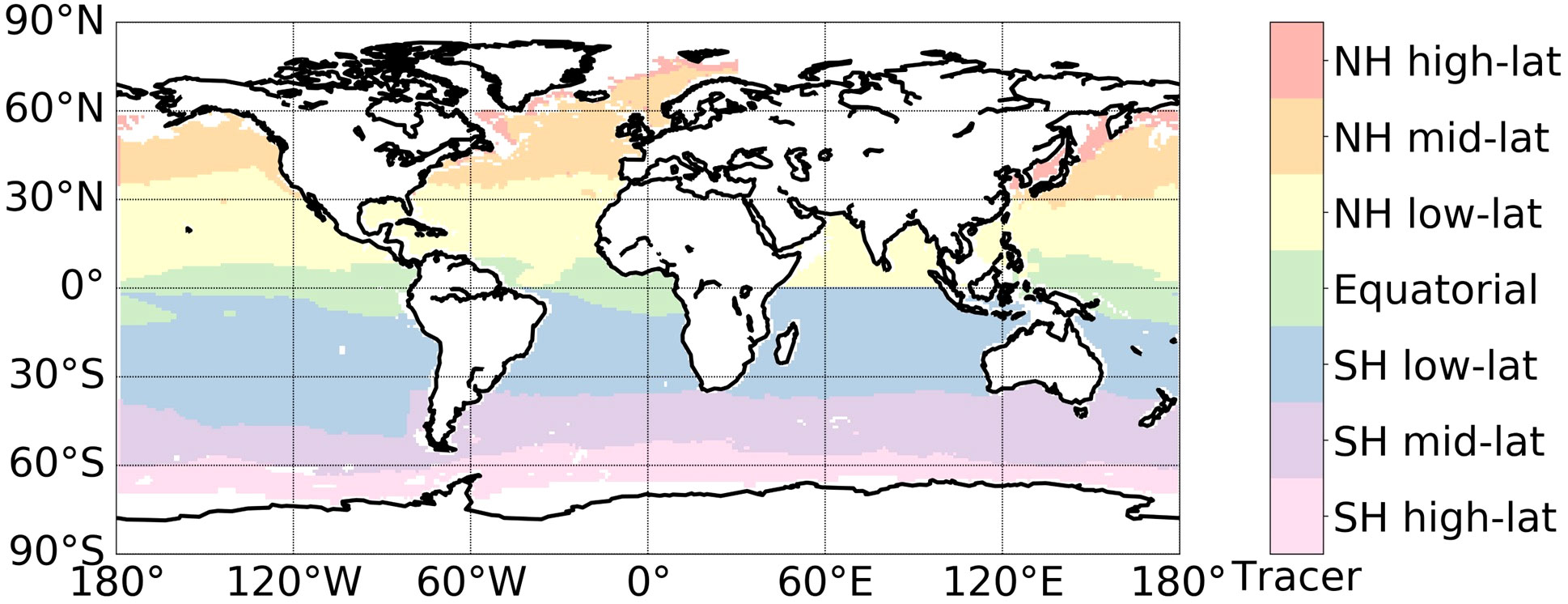
Figure 1 The tracers defined for the tagged simulations based on ocean biome regions in Fay et al., 2014.
2.1.2 OCO-2 observations
We analyze IAV in dry air, column-average mole fraction XCO2 inferred from OCO-2 satellite observations. The OCO-2 observatory was launched in July 2014 and has measured passive, reflected solar near-infrared CO2 and O2 absorption spectra using grating spectrometers since September 2014 (Eldering et al., 2017). XCO2 data are retrieved from the measured spectra using the Atmospheric CO2 Observations from Space (ACOS) optimal estimation algorithm, which is a full physics algorithm that solves for XCO2 and other physical parameters, including surface pressure, surface albedo, temperature, and water vapor profile in its state vector (O’Dell et al., 2018). The satellite is in a polar and sun-synchronous orbit that repeats every 16 days, with three different observing modes of OCO-2, namely nadir (land only, views the ground directly below the spacecraft with insufficient signal to noise over the ocean), glint (ocean and land, views the spot with directly reflected sunlight resulting in a higher ocean signal), and target (sites of specific interest, primarily for validation) (Crisp et al., 2012, 2017). We use the version 10 OCO-2 Level 2 bias-corrected XCO2 data product from 2014 September to 2022, (From Goddard Earth Sciences Data and Information Services Center Archive: https://disc.gsfc.nasa.gov/datasets/OCO2_L2_Lite_FP_10r/summary), which has been validated with collocated ground-based measurements from the Total Carbon Column Observing Network (TCCON). After filtering and bias correction, the OCO-2 XCO2 retrievals agree well with TCCON in nadir, glint, and target observation modes, and generally have absolute median differences less than 0.4 ppm and RMS differences less than 1.5 ppm (O’Dell et al., 2012; Wunch et al., 2017).
We characterize IAV from OCO-2 XCO2 in Guan et al. (2023). In that analysis, we determined optimal spatiotemporal scales for aggregating the observations to detect IAV variability in light of other sources of error. We evaluated IAV signals against the TCCON ground-truth network, confirming that the IAV inferred from OCO-2 is robust given the small magnitude of IAV compared to other sources of variance (Mitchell et al., 2023). Further, the OCO-2 IAV timeseries show similar zonal patterns of OCO-2 XCO2 IAV timeseries compared to GOSAT space-based observation and ground-based NOAA ESRL in situ data. The analysis by Guan et al. (2023) validates that the OCO-2 satellite provides new capabilities for discerning atmospheric XCO2 IAV.
2.2 Methods
2.2.1 GEOS-Chem simulations
We simulate atmospheric XCO2 generated by ocean carbon fluxes using GEOS-Chem (Bey et al., 2001), an offline global chemical transport model driven by meteorological input from the Goddard Earth Observing System (GEOS) of the NASA Global Modeling and Assimilation Office (GMAO) and developed by an extensive global community of researchers. It has been widely used for gas flux inversion and source attribution studies, including for CO2, CH4, and CO (e.g., Nassar et al., 2010; Fisher et al., 2017). We use the version 12.0.0 of GEOS-Chem, released in Aug 2018.
To simulate atmospheric CO2 fields from individual subregions, we modify the GEOS-Chem code base to tag the source regions and separately track different CO2 tracers originating from each region (Lin et al., 2020). This approach is possible since CO2 is a passive tracer that is not involved in atmospheric chemical reactions. In the simulation, each CO2 tracer corresponds to the influence of ocean CO2 fluxes from one tagged region, and the simulation using the JENA product has two more tracers than SOMFFN and CMEMS since the JENA product has slightly larger data coverage in both the far North and the far South.
The meteorological inputs for GEOS-Chem come from the Modern-Era Retrospective analysis for Research and Applications, 80 Version 2 (MERRA2) reanalysis. We run simulations for 1982-2021 at 2° latitude by 2.5° longitude resolution with 47 vertical levels up to 0.01 hPa on a hybrid eta (sigma-pressure) grid. The ocean flux products were rescaled to 2° latitude by 2.5° longitude resolution using the GEOS-Chem rescaling module. Convective transport in GEOS-Chem is simulated with a single-plume scheme (Wu et al., 2007) while boundary layer mixing in GEOS-Chem uses the non-local parameterization (Lin and McElroy, 2010) which draws on the mixing depths, temperature, latent and sensible heat fluxes, and specific humidity. Although some bias in the vertical distribution of CO2 has been shown in GEOS-Chem for northern high latitudes (Schuh et al., 2019), similar tagged transport runs have been shown to generally capture seasonal cycles in surface CO2 as well as gradients between surface and mid-tropospheric CO2 across a range of latitudes (Lin et al., 2020). The model is initialized with a globally-uniform atmospheric CO2 mole fraction equal to 350 ppm and allowed to spin-up for 3-years using cyclostationary ocean fluxes. Time-varying ocean fluxes are then applied beginning in 1982. We calculate XCO2 in the GEOS-Chem runs by integrating the dry air mole fraction for the 47 model layers accounting for pressure differences with height. Because we are interested in isolating the impact of ocean-atmosphere CO2 exchange, we do not simulate the imprint of either fossil or terrestrial biospheric CO2 exchange on XCO2.
In a sensitivity study, we isolate the impact of atmospheric transport IAV, rather than air-sea flux IAV, on the resulting IAV in XCO2. For this analysis, we simulate XCO2 from the seasonal climatology of air-sea CO2 fluxes averaged over the 40-year period of the GEOS-Chem simulation, maintaining time-varying atmospheric transport from the MERRA2 reanalysis. Together with the baseline experiment using time-varying air-sea fluxes and time-varying transport, we can distinguish the effect of dynamical-driven variation, flux-driven variation, and the combination of both.
2.2.2 Timeseries analysis
We characterize spatiotemporal patterns of OCO-2 detected XCO2 by first aggregating OCO-2 observations to monthly averages on a 5° by 5° grid equatorward of 45° and to a 5° by 10° grid poleward of 45° from 2014.08 (August) to 2021, which overlaps with the simulation time period. Our analysis shows that averaging XCO2 observations at these scales minimizes the effect of retrieval error and mitigates influences caused by missing measurements due to cloud cover in the tropics and weak winter sunlight in polar regions (Guan et al., 2023). We similarly aggregate GEOS-Chem model output at this scale when compared to OCO-2. We use a consistent process to calculate IAV from the OCO-2 XCO2 (Equation 1), and GEOS-Chem XCO2 (Equation 2), but we note that we must account for an additional term in the multi-decadal GEOS-Chem simulations since curvature in the long-term atmospheric growth trend must be taken into account. The methodology is based on approaches used in Keppel-Aleks et al. (2014) and NOAA curve fitting methodology (Thoning et al., 1989).
In these equations, (x,y) denotes a specific gridcell, t denotes a specific time, and m denotes a monthly average. We first fit a third-order polynomial to the Raw timeseries to calculate the trend at each location. For the GEOS-Chem simulation, since polynomial fitting does not fully capture the long-term trend over multiple decades, we apply a Fast Fourier Transform 10-year low-pass filter to remove decadal-scale variability. We calculate a mean seasonal cycle by taking the average value of all January, February, etc. data after removing the long-term trends. Finally, we remove the mean seasonal cycle from the detrended timeseries at each gridcell to obtain the IAV anomaly timeseries. We calculate the IAV amplitude as the standard deviation of the IAV anomaly timeseries. An identical method is used to calculate IAV from the gridded fluxes.
3 Results
Figure 2 shows the global distribution of air-sea CO2 flux IAV amplitude (calculated as the standard deviation of IAV anomalies) over 40 years from 1982 to 2021 in the observation-based products. The three observation-based products show broadly similar magnitudes and spatial patterns in air-sea flux IAV in the Northern Hemisphere and Southern Hemisphere low to mid latitudes (Supplementary Figure S3). The flux IAV amplitude is highest over the northern midlatitude ocean, Eastern Pacific, and Southern Ocean, with the largest inter-product differences in the northern hemisphere. In the Southern Hemisphere, the zonally integrated air-sea flux IAV is largest at 60°, around 0.6-0.7 mol m-2 y-1. The flux IAV decreases by almost a factor of three in the subtropical regions in both hemispheres to around 0.2 mol m-2 s-1. The large zonal IAV and the small zonal standard deviation around a latitude circle in the Southern Ocean, especially for SOMFFN and CMEMS (shading in Figures 2D, F), is due to the fact that in the Northern Hemisphere, though there is larger flux IAV amplitude (solid blue line in Figures 2D–F), there is also more variability from gridcell to gridcell (shaded blue area in Figures 2D–F). Thus, the gridcell-level variability partially cancels when integrated around a latitude band, leading to a smaller northern ocean impact on atmospheric XCO2. Consequently, the Southern Hemisphere has a bigger imprint of atmospheric XCO2 IAV, as we will show below.
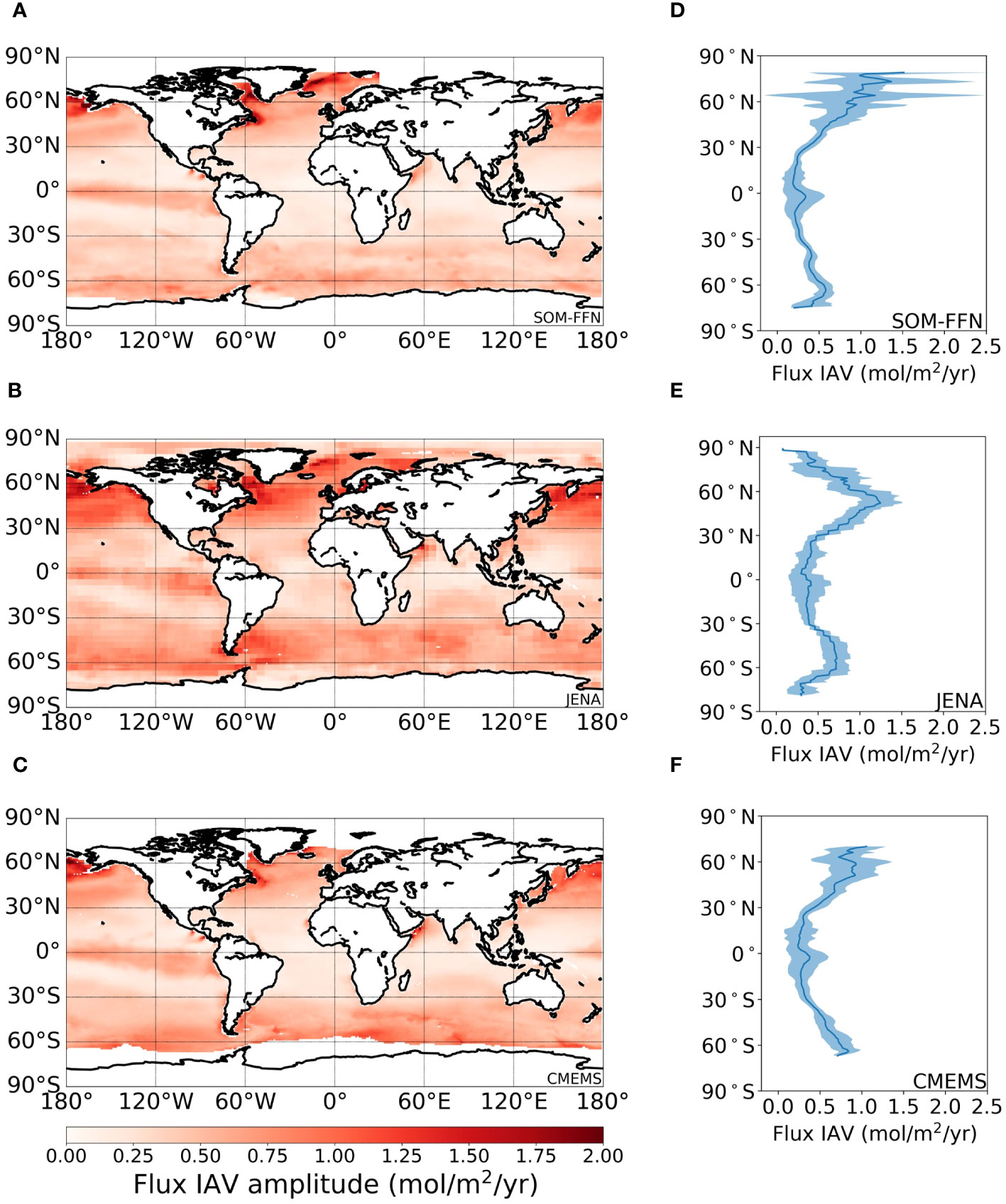
Figure 2 Map of ocean flux IAV amplitude (A–C) and latitudinal profile of zonal mean flux IAV amplitude (D–F). More intense colors signify more IAV while lighter colors indicate lower IAV regions. The IAV amplitude is calculated from the standard deviation of the IAV timeseries. The zonal mean IAV is obtained by averaging the IAV timeseries for all longitudes within the specified latitude band, while the shading shows the standard deviation of the IAV timeseries among all longitudes, indicating the coherence of flux IAV around a latitude circle. (A, D) show results for SOMFFN; (B, E) show results for JENA and (C, F) show results for CMEMS (E, F) product.
The XCO2 timeseries simulated from global air-sea fluxes (i.e., the sum of all tagged regions) shows IAV that ranges from +/-0.2 ppm for JENA (Figure 3) with smaller variations from +/-0.1 ppm for SOM-FFN and CMEMS. The IAV from the products is small compared with the OCO-2 XCO2 IAV (Guan et al., 2023). Both spatially averaged timeseries (Figure 3) and maps of IAV (Supplementary Figure S4) are notably different across the three observation-based flux products when propagated through an atmospheric transport model. The simulated XCO2 from JENA is different compared to that derived from the other two observation-based flux products, due to differences especially in the Southern Hemisphere fluxes. We note, however, that XCO2 simulated from any one flux product is generally coherent across latitude bands. The corresponding globally averaged XCO2 IAV amplitude is about 0.11 ppm for JENA, but less than 0.07 ppm for SOMFFN and CMEMS (Figures 4A–C). Each data product shows the ocean-driven XCO2 IAV amplitude largest over the tropical Pacific and the Southern Ocean. When the IAV amplitude is calculated for the period from September 2014 to 2021, the overlapping period between OCO-2 observations and observation-based products, the amplitude is similar for SOMFFN and JENA (around 0.12 ppm globally averaged), and similar for CMEMS (around 0.08 ppm). The difference in simulated IAV for a given observation-based product calculated across two different time periods suggests that the ocean may leave a larger imprint on XCO2 IAV in recent years compared to historical averages.
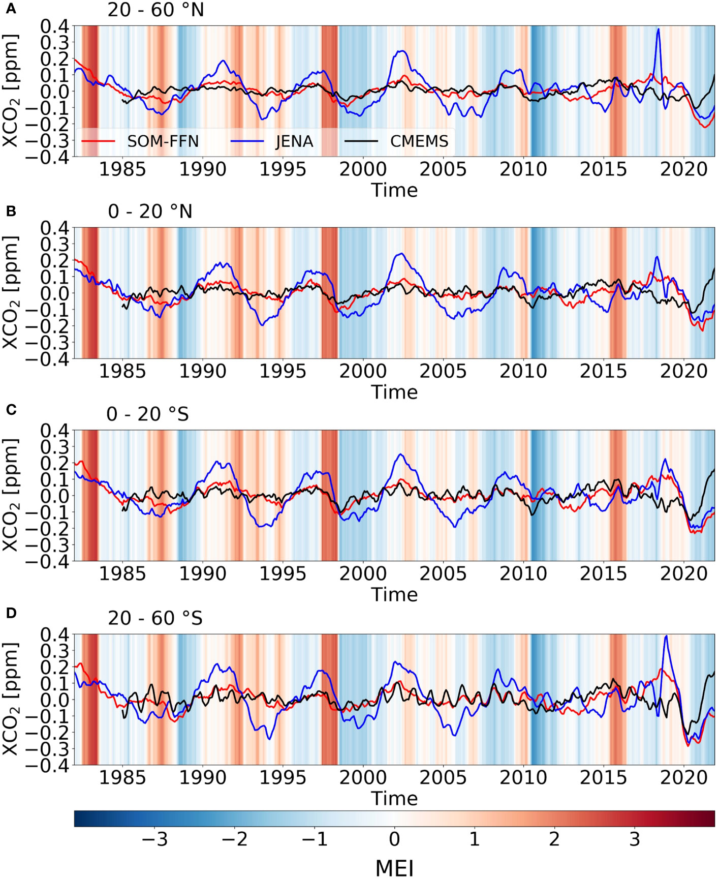
Figure 3 Ocean XCO2 IAV timeseries averaged for zonal bands from three different observation-based products. (A) 20 – 60°N, (B) 0 – 20°N, (C) 0 – 20°S, (D) 20 – 60°S. The background shading indicates the Multivariate ENSO Index (MEI), which is positive during El Niño phases.
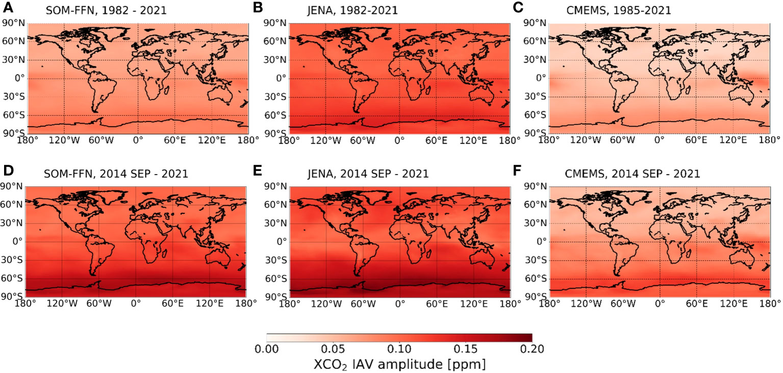
Figure 4 Ocean XCO2 IAV amplitude based on simulation from 1982 to 2021 (top row) and during the period of overlap with OCO-2 (September 2014 through the end of 2021) (bottom row) using (A, D) SOMFFN (B, E) JENA and (C, F) CMEMS ocean observation-based products as input surface CO2 fluxes to GEOS-Chem atmospheric transport runs.
The Southern Hemisphere oceanic regions are the dominant contributors to XCO2 IAV across the three models. We calculated the XCO2 IAV amplitude arising separately from each regional tracer, then determined the region that contributes the largest and second largest IAV amplitude to each global atmospheric gridcell (left-hand column of Figure 5 and Supplementary Figures S5–7). Across all three models, the Southern Hemisphere low- and mid-latitude regions are the primary contributors to IAV over 70-95% of the global area (Table 1), including large swaths of the Northern Hemisphere for SOMFFN and CMEMS. In fact, the SOMFFN simulation shows that Northern Hemisphere ocean regions are not a dominant contributor to XCO2 IAV even locally. In contrast, the XCO2 IAV from the simulation with JENA and CMEMS fluxes show a modest contribution from the Northern Hemisphere, with the mid latitude region emerging as the dominant contributor to about 15% of the global area. The dominant region in each gridcell accounts for up to 60% of the atmospheric XCO2 IAV amplitude for CMEMS (Figure 5F), and roughly 35-50% of the IAV amplitude for SOMFFN and JENA (Figures 5B, D), suggesting more equable contributions from different regions. The second most-dominant contributors to atmospheric CO2 IAV are similarly the Southern Hemisphere, or tropics or Northern Hemisphere mid-latitude across all three ocean-flux-GEOS-Chem simulations (Table 2).
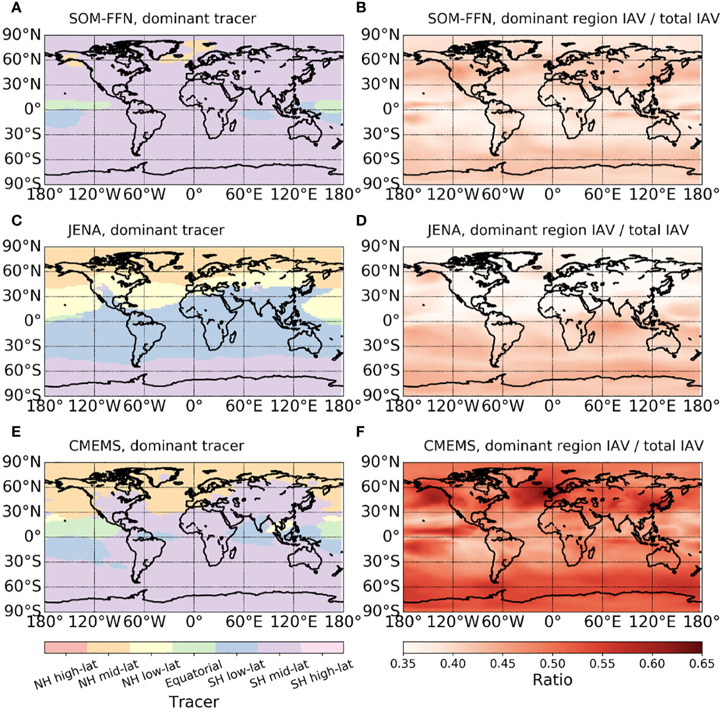
Figure 5 The most influential ocean subregions at different locations based on simulations from 1982 to 2021 with time-varying (A) SOMFFN, (C) JENA, and (E) CMEMS fluxes. The dominant tracer is identified by calculating the XCO2 IAV amplitude for each gridcell caused by a single tracer and then ranking them. The fraction of the overall IAV amplitude accounted for by the dominant tracer is shown in the right-hand column for (B) SOMFFN, (D) JENA, and (F) CMEMS.
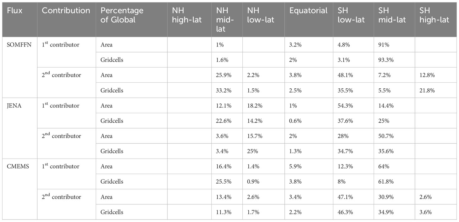
Table 1 The percentage of global area or global gridcells for which each ocean flux region is the dominant driver of IAV in simulations with time-varying ocean fluxes and time-varying atmospheric transport.
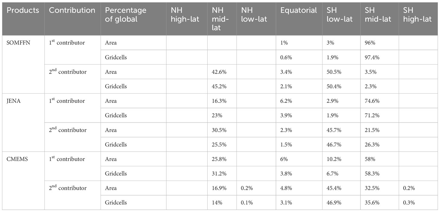
Table 2 Same as Table 1, except for simulations with cyclostationary ocean fluxes and time-varying atmospheric transport.
Not all IAV in XCO2 arises from IAV in local surface fluxes; IAV in patterns of atmospheric transport is also an important contributor to XCO2 IAV. We calculate the relative contributions of ocean flux variability and IAV in atmospheric transport from GEOS-Chem simulations with climatological monthly-mean cyclostationary ocean CO2 fluxes as surface boundary conditions. IAV in these simulations arises only from IAV in atmospheric transport acting on the spatial gradients in XCO2 set up by the climatological annual cycle of ocean air-sea CO2 exchange. All three products show nearly identical spatial patterns in the XCO2 amplitude arising from cyclostationary air-sea CO2 fluxes (Figures 6A–C), suggesting that seasonal flux patterns result in similar atmospheric gradients (Landschtzer et al., 2023) across the three models. The western Pacific warm pool is a hotspot for dynamics-driven variability, likely due to ENSO-driven changes in atmospheric transport, and this region has an IAV amplitude of 0.07-0.08 ppm across all three simulations. Given the large variability in the magnitude of IAV among SOMFFN, JENA, and CMEMS (Figure 4), the ratio of dynamics-driven variations to total IAV diverged among the ocean-flux-GEOS-Chem simulations (Figures 6D–F). For SOMFFN and CMEMS, which showed smaller IAV when driven with interannually varying fluxes, transport contributes about 50% of IAV in the Southern Hemisphere subtropics and subpolar regions, and 50-80% of IAV in the tropics and high latitudes of both hemispheres. For JENA, which had high IAV in the full simulations (Figure 4B), transport contributes less than 20% of total IAV except in the tropical Pacific, where it contributes 50%.
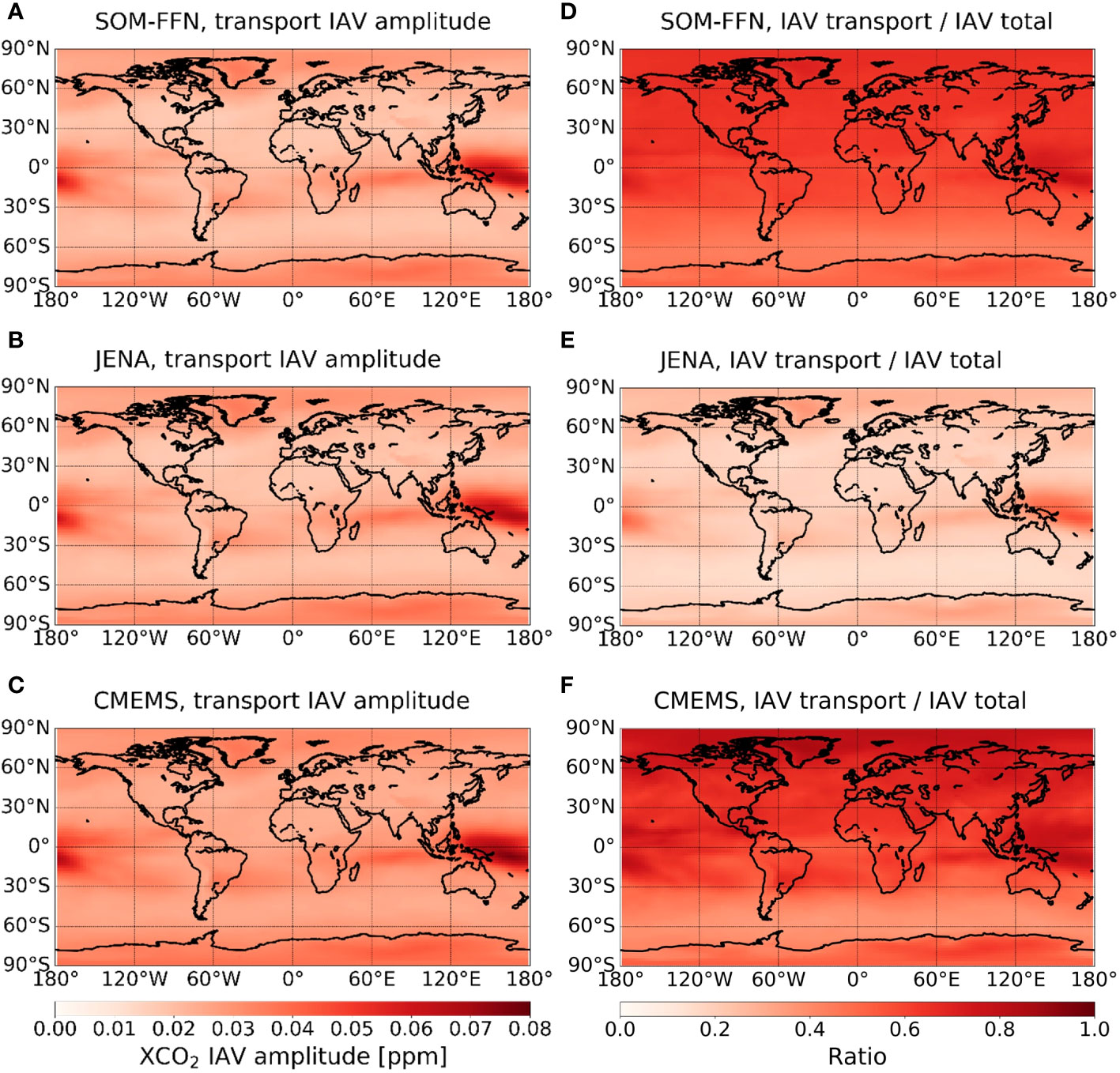
Figure 6 The ocean XCO2 IAV amplitude from transport-only simulations based on (A) SOMFFN, (B) JENA, and (C) CMEMS. The ratio of total IAV generated by transport alone for (D) SOMFFN, (E) JENA, and (F) CMEMS.
In the atmospheric transport simulations with cyclostationary fluxes, the Southern Hemisphere mid-latitude region is the dominant contributor to IAV for about 60% to 96% of the global area. Consistent across the three observation-based products, the second dominant contributor is the Southern Hemisphere low-latitude region. These results suggest that IAV in transport interacts most strongly with atmospheric gradients set up by Southern Hemisphere fluxes. JENA and CMEMS show that the Northern Hemisphere mid latitude regions are also important contributors when run with cyclostationary fluxes, and are the dominant contributor to roughly 15% to 25% of the global area. Figure 7 shows that in the cyclostationary simulations, the influence of Northern and Southern Hemisphere regions are more localized to the originating hemisphere. Taken together with the results from the time-varying fluxes, these results suggest that IAV in the Southern Hemisphere fluxes is synergistic with IAV from atmospheric transport, whereas, in the Northern hemisphere, IAV in the fluxes counteracts the IAV due to transport alone.
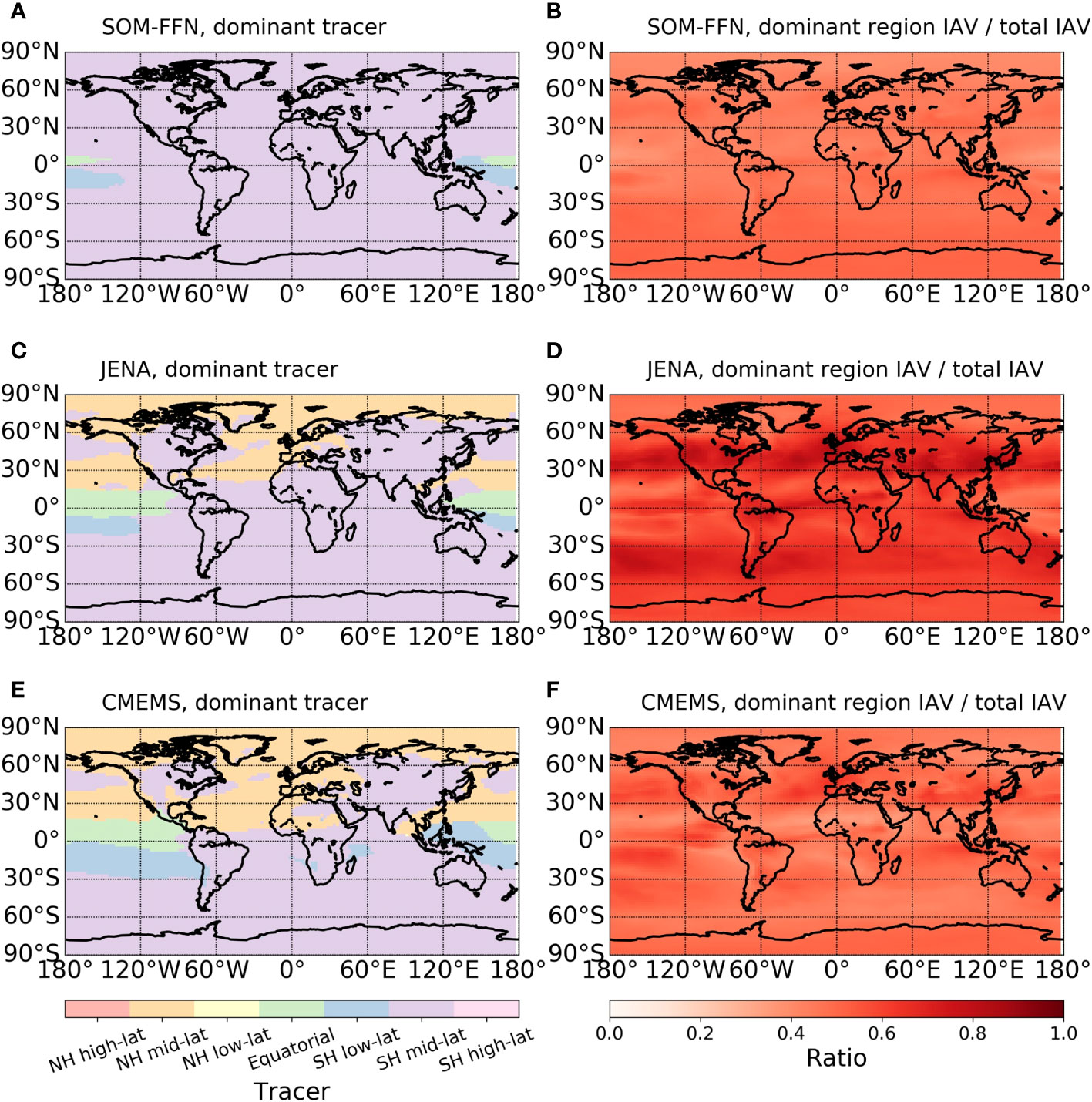
Figure 7 The most influential ocean subregions at different locations based on simulations with cyclostationary (A) SOMFFN, (C) JENA, and (E) CMEMS ocean fluxes. The dominant tracer is identified by calculating the XCO2 IAV amplitude for each gridcell caused by each region and then ranking them. The fraction of the overall IAV amplitude accounted for by the dominant region is shown in the right-hand column for (B) SOMFFN, (D) JENA, and (F) CMEMS.
The ocean-driven XCO2 IAV simulated by the three observation-based products is largely unrelated to observed patterns of IAV as observed by OCO-2, which includes other sources of IAV. The OCO-2 IAV amplitude, which is of order 1 ppm for the 2014-2021 period, was an order of magnitude larger than that simulated from any of the three-ocean observation-based products which is of order 0.1ppm (Figures 4, 8). A possible explanation could be that the OCO-2 observations contain the imprint not only of ocean fluxes but also land and fossil emissions. The OCO-2 XCO2 IAV amplitude, calculated as the standard deviation of the IAV timeseries, suggests that XCO2 interannual variability over ocean basins is smaller than that over continents (around 0.4 ppm vs 1.2 ppm; Figure 8), although this may be due to larger error variance due to complex topography and land surface albedo variations (Guan et al., 2023; Mitchell et al., 2023). We calculate the correlation coefficient, slope, and fractional ratio between simulated XCO2 IAV and OCO-2 XCO2 IAV (Figure 9, Supplementary Figure S8) at the gridscale to explore where the imprint of the ocean might be detectible. Over most of the planet, the observed XCO2 IAV is only weakly correlated with the XCO2 IAV simulated from ocean fluxes, with many regions showing a slight negative correlation. These correlations are generally not statistically significant, with p>0.05. Simulations from the three different flux products show different meridional patterns of correlation, with JENA simulations showing slight positive correlations within the tropics and CMEMS showing slight positive correlations in the Southern Hemisphere, although we note these relationships are not statistically significant. Across all regions, the slope between the observed and simulated XCO2 IAV is less than 0.2 units? (Figures 9D–F), consistent with the magnitude of the observed IAV being dominated by terrestrial signals. The maps of correlations and slopes suggest that detecting ocean IAV directly from space-based measurements is challenging given other sources of variability. Disentangling these multiple impacts to differentiate between plausible ocean flux products, such as the three analyzed here, will require a combination of observations and modeling.
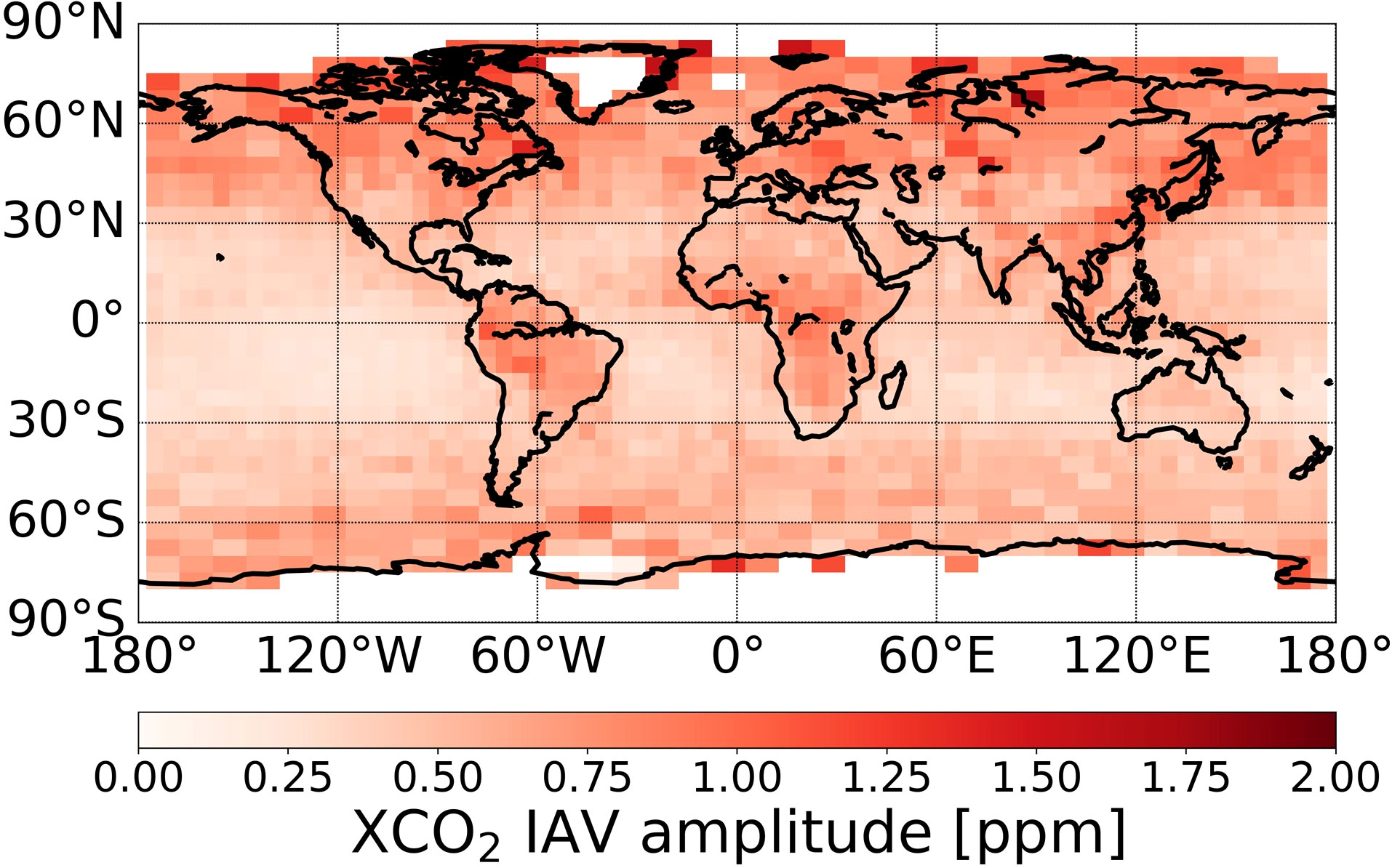
Figure 8 Observed OCO-2 XCO2 IAV amplitude, determined as the standard deviation of the IAV timeseries. Data equatorward of 45° are averaged at 5° by 5° resolution, and data poleward of 45° are averaged at 5° by 10° resolution based on Guan et al. (2023).
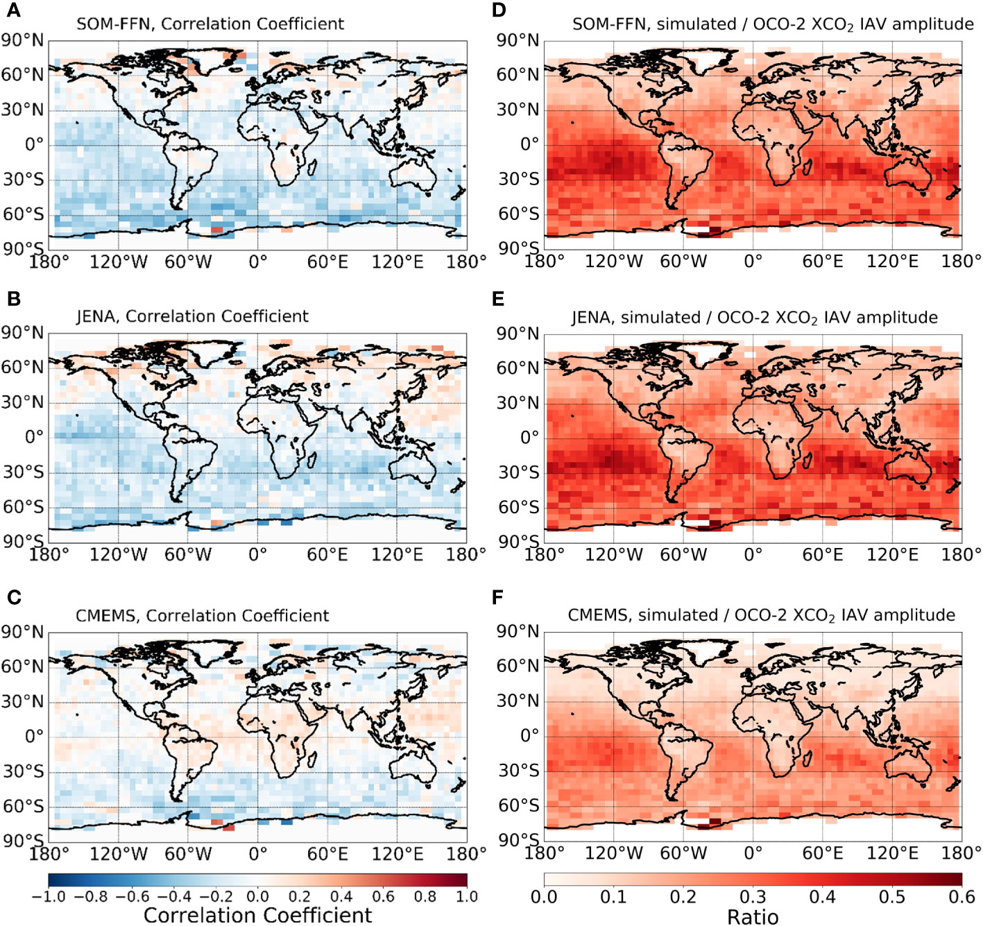
Figure 9 (A–C) The correlation coefficient between simulated ocean XCO2 IAV and OCO-2 IAV for (A) SOMFFN, (B) JENA, and (C) CMEMS data products. (D-F) The ratio of IAV amplitude between simulated oceanic XCO2 IAV and OCO-2 XCO2 IAV, for (D) SOMFFN, (E) JENA, (F) CMEMS.
Previous analysis of OCO-2 observations over the tropical Pacific suggested that space-based observations can detect an ocean-driven decrease in XCO2, potentially as large as 0.5 ppm, during the initial phases of the strong 2015 El Niño (Chatterjee et al., 2017). Our simulations show that atmospheric XCO2 decreases over the Nino 3.4 region during the strong 1997-1998 El Niño (by about 0.3 ppm), but show a weaker decrease (about 0.1ppm) during 2015-2016 El Niño. The decrease in the atmospheric XCO2 IAV timeseries corresponds to the reduced ocean outgassing over the Niño 3.4 region (up to 1.5 mol/m2/y) (Figure 10), which is roughly similar between the two El Niño periods and leads to similar decreases in the tropical XCO2 tracer (Supplementary Figure S9). During the strong 1997-98 El Niño, however, a temporary reduction in Northern Hemisphere CO2 outgassing also reduced XCO2 over the Niño.4 region, amplifying the apparent response (Supplementary Figure S9). As expected, XCO2 anomalies during the two El Niño events are mainly driven by changes in the air-sea CO2 flux rather than changes in the atmospheric circulation (Supplementary Figure S10). However, these flux-driven anomalies are small (less than +/- 0.03 ppm). Our simulations suggest that even during strong El Niño events, detecting the direct atmospheric imprint of changes in ocean outgassing within the tropics will be challenging given the small direct signal predicted from all three observational flux products, compounding variability from other ocean and terrestrial regions, and retrieval uncertainties in XCO2.
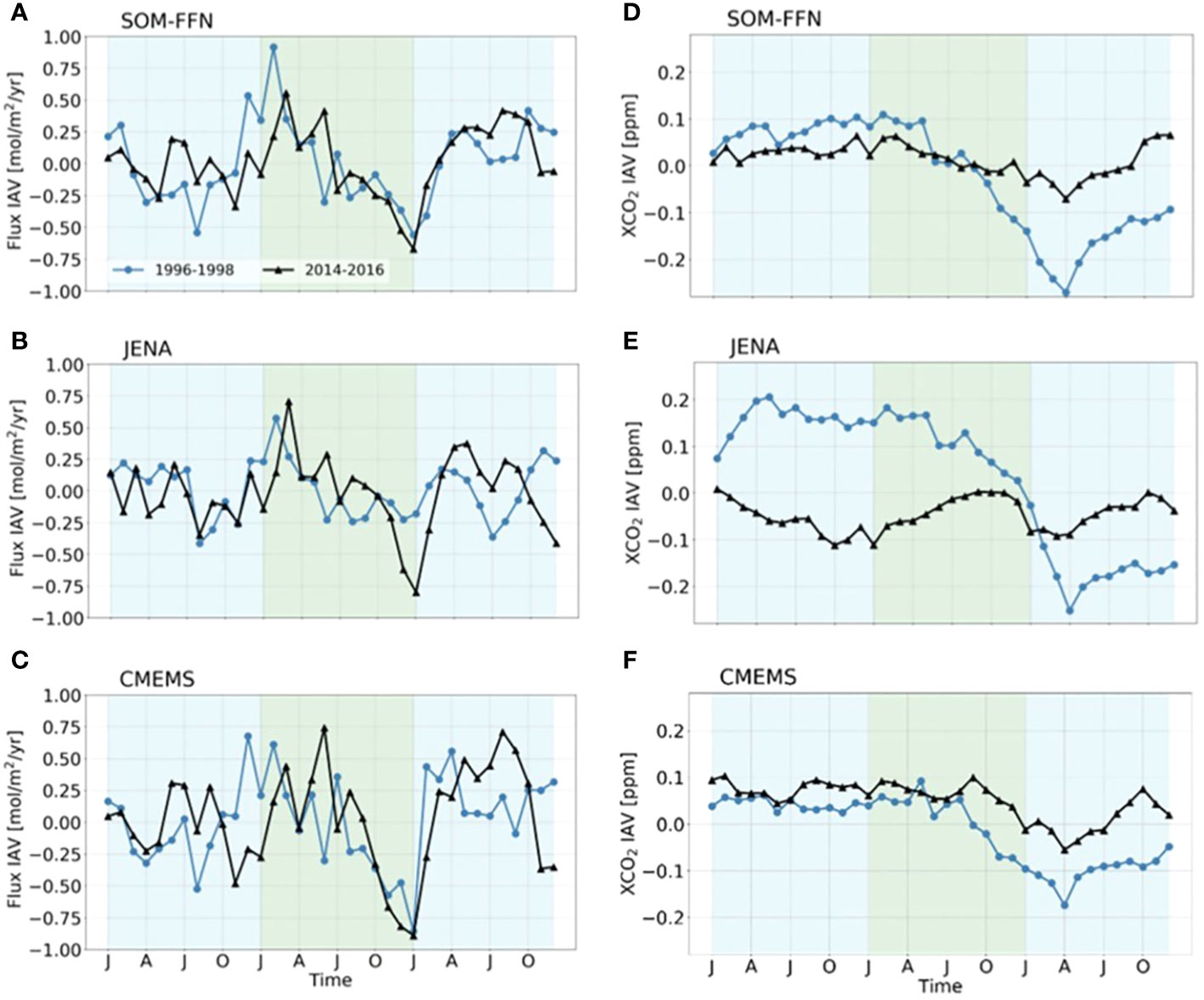
Figure 10 Ocean IAV timeseries averaged over the Niño 3.4 region for three years centered on two strong El Niño events: 1997-1998 in blue; 2015-2016 in black. Year 1 and Year 3 are shaded blue, and Year 2 is shaded with green. Left Column shows the Ocean Flux IAV whereas the right column shows the simulated ocean XCO2 IAV. (A, D) SOMFFN, (B, E) JENA, (C, F) CMEMS.
4 Discussion
We simulate ocean-driven IAV in atmospheric CO2 based on three estimates of air-sea CO2 fluxes from interpolated observation-based products. Although these observation-based products all use the same ocean pCO2 data to estimate gridded fluxes and show largely similar spatial patterns of flux IAV, they result in very different estimates of atmospheric XCO2 IAV over the 40 year period from 1982-2021 (Figures 3, 4A–C). The inter-model spread was much reduced when looking at the four years from 2014-2021 overlapping with OCO-2 observations (Figures 4D–F). Our results largely corroborate the results from Nevison et al. (2008), who showed a small imprint for the ocean on atmospheric CO2 IAV. Our results show that even in the remote Southern Ocean, which shows large IAV in the fluxes, the atmospheric IAV signature imparted by the ocean is small.
Further, our simulations show that up to 80 percent of the IAV of the IAV in atmospheric XCO2 results from IAV in atmospheric transport acting on atmospheric gradients derived from cyclostationary ocean fluxes (Figure 6), not from IAV in the ocean fluxes themselves. The three observation-based products showed a very similar pattern of transport-induced IAV, with the dominant spatial contributors (SH low-lat and SH mid-lat) showing high consistency among the three data products (Table 1). This is somewhat expected, since the MERRA/GEOS-Chem atmospheric transport patterns were common among all three simulations, but also requires that the three observation-based products provide similar mean spatial seasonal patterns in oceanic CO2 fluxes (Supplementary Figure S11).
Our study shows that atmospheric XCO2 IAV is affected most strongly by air-sea CO2 fluxes in the Southern Hemisphere (Figure 7), although the observation-based products show tradeoffs between the Southern Hemisphere low- and mid-latitude regions in terms of which region dominates. In the simulations with time-varying air-sea fluxes, the Southern Hemisphere, and to a lesser extent the tropics, dominate ocean-driven XCO2 IAV even in the Northern Hemisphere. This pattern generally holds in the simulations with cyclostationary fluxes, although the Northern Hemisphere regions have a relatively larger contribution.
Given the small signature of ocean fluxes on atmospheric XCO2 IAV, attributing ocean-induced IAV based on space-based observations will be challenging. Mitchell et al. (2023) provide a detailed assessment of time and space scales of variation in OCO-2 XCO2 over North American land and coastal ocean using a geostatistical approach. They identify synoptic scale variations as contributing up to 2 ppm2 variance, mesoscale transport, and correlated error as contributing up to 1 ppm2 variance, and random noise as up to 1 ppm. Given that our simulations suggest the imprint of ocean IAV is less than 0.1 ppm, these results suggest that directly observing ocean IAV is not possible with the current technology for space-based remote sensing of atmospheric CO2. Rather, XCO2 observations will require precision better than 0.1 ppm, or 0.025% on a ~400 ppm background to detect and attribute ocean-driven variation.
Furthermore, because transport is an important contributor to the patterns of atmospheric CO2 IAV, using methods such as atmospheric inversions to back out ocean fluxes in an optimal estimation framework requires fidelity in atmospheric transport modeling (Schuh et al., 2019). Here, patterns of atmospheric transport-induced IAV from cyclostationary air-sea CO2 fluxes (Figure 6) are similar because all flux products were transported through the same GEOS-Chem transport model. The choice of a different transport model would likely result in different spatial patterns, albeit with a similarly small magnitude compared to the IAV amplitude of the observations.
During the four years from 2014-2021 overlapping with OCO-2 observations, all three observation-based flux products show a multi-year decrease in the net ocean flux. There is low correspondence between the simulated XCO2 IAV driven by ocean fluxes with total IAV detected from OCO-2. We hypothesize that multi-decadal variability in air-sea CO2 fluxes may be more detectable in atmospheric XCO2 than the year-to-year variability presented here, but testing this hypothesis requires ongoing space-based observations of XCO2.
Our results temper the optimistic results from Chatterjee et al. (2017), who showed that a large ocean flux signal could be discerned from space-based XCO2 data. Our study shows that the Southern Hemisphere oceans were the largest ocean-driven XCO2 IAV in our simulations (Figure 4), and that tropical Pacific that was most sensitive to IAV in atmospheric transport (Figure 6).
Nevertheless, all three ocean products we analyze suggest a smaller XCO2 IAV than what was observed for the 2015-16 El Niño. These results suggest that flux anomalies associated with changing modes in ocean oscillations in other basins may impart smaller variations in the atmosphere that are difficult to detect using OCO-2 or a similar satellite.
5 Conclusions
We evaluate the imprint that air-sea CO2 fluxes from the whole ocean and different oceanic subregions leave on the atmospheric XCO2 interannual variation. We simulate ocean-driven XCO2 using the GEOS-Chem atmospheric transport model and air-sea CO2 fluxes estimated from observation-based surface pCO2 products and compare against the observed total XCO2 IAV based on OCO-2 column-mean CO2 observation from late 2014 to 2022. The ocean-driven IAV amplitude (standard deviation) in atmospheric XCO2 caused by air-sea CO2 exchange and IAV in atmospheric transport is generally between 0.08 and 0.12 ppm. While this magnitude is up to 40% of the total IAV in OCO-2 XCO2 over the tropical and subtropical ocean basins, it is well below random noise in individual OCO-2 soundings and systematic errors in the satellite observations themselves. These results indicate that direct observation of air-sea CO2 flux variations from total column XCO2 would be very challenging with current space-based sensors.
Data availability statement
The raw data supporting the conclusions of this article will be made available by the authors, without undue reservation.
Author contributions
YG: Conceptualization, Data curation, Formal analysis, Investigation, Methodology, Software, Visualization, Writing – original draft, Writing – review & editing. GM: Conceptualization, Funding acquisition, Methodology, Project administration, Resources, Supervision, Validation, Writing – review & editing. AF: Conceptualization, Data curation, Methodology, Resources, Software, Writing – review & editing. SD: Conceptualization, Funding acquisition, Methodology, Project administration, Resources, Supervision, Writing – review & editing, Validation. GK: Conceptualization, Funding acquisition, Methodology, Project administration, Resources, Supervision, Validation, Writing – original draft, Writing – review & editing.
Funding
The author(s) declare financial support was received for the research, authorship, and/or publication of this article. We acknowledge NASA support through the OCO Science team and the Interdisciplinary Science Program and NASA awards 80NSSC18K0900, 80NSSC21K1070, and NNX17AK19G to the University of Michigan; awards 80NSSC18K0897 and 80NSSC21K1071 to the University of Virginia, and award 80NSSC22K0150 to Columbia University.
Acknowledgments
The authors thank the participants of the NASA OCO-2 mission for providing the OCO-2 data product (From GES DISC Archive: https://disc.gsfc.nasa.gov/datasets/OCO2_L2_Lite_FP_10r/summary) used in this study.
Conflict of interest
The authors declare that the research was conducted in the absence of any commercial or financial relationships that could be construed as a potential conflict of interest.
Publisher’s note
All claims expressed in this article are solely those of the authors and do not necessarily represent those of their affiliated organizations, or those of the publisher, the editors and the reviewers. Any product that may be evaluated in this article, or claim that may be made by its manufacturer, is not guaranteed or endorsed by the publisher.
Supplementary material
The Supplementary Material for this article can be found online at: https://www.frontiersin.org/articles/10.3389/fmars.2024.1272415/full#supplementary-material
References
Ballantyne A. P., Alden C. B., Miller J. B., Tans P. P., White J. W. C. (2012). Increase in observed net carbon dioxide uptake by land and oceans during the past 50 years. Nature 488, 70–72. doi: 10.1038/nature11299
Bennington V., Gloege L., McKinley G. A. (2022). Variability in the global ocean carbon sink from 1959 to 2020 by correcting models with observations. Geophysical Res. Lett. 49, e2022GL098632. doi: 10.1029/2022GL098632
Bey I., Daniel J., Yantosca R. M., Logan J. A., Field B. D., Fiore A. M., et al. (2001). Global modeling of tropospheric chemistry with assimilated meteorology: Model description and evaluation. J. Geophys. Res. Atmos. 106, 23073–23095. doi: 10.1029/2001JD000807
Buchwitz M., Reuter M., Schneising O., Noël S., Gier B., Bovensmann H., et al. (2018). Computation and analysis of atmospheric carbon dioxide annual mean growth rates from satellite observations during 2003–2016. Atmospheric Chem. Phys. 18, 17355–17370. doi: 10.5194/acp-18-17355-2018
Chatterjee A., Gierach M. M., Sutton A. J., Feely R. A., Crisp D., Eldering A., et al. (2017). Influence of El Niño on atmospheric CO2 over the tropical Pacific Ocean: Findings from NASA’s OCO-2 mission. Science 358, eaam5776. doi: 10.1126/science.aam5776
Crisp D., Dolman H., Tanhua T., McKinley G. A., Hauck J., Bastos A., et al. (2022). How well do we understand the land-ocean-atmosphere carbon cycle? Rev. Geophysics 60, e2021RG000736. doi: 10.1029/2021RG000736
Crisp D., Fisher B. M., O’Dell C., Frankenberg C., Basilio R., Bösch H., et al. (2012). The ACOS CO2 retrieval algorithm – Part II: Global XCO2 data characterization. Atmos. Meas. Tech. 5, 687–707. doi: 10.5194/amt-5-687-2012
Crisp D., Pollock H. R., Rosenberg R., Chapsky L., Lee R. A. M., Oyafuso F. A., et al. (2017). The on-orbit performance of the Orbiting Carbon Observatory-2 (OCO-2) instrument and its radiometrically calibrated products. Atmos. Meas. Tech. 10, 59–81. doi: 10.5194/amt-10-59-2017
Denvil-Sommer A., Gehlen M., Vrac M., Mejia C. (2019). LSCE-FFNN-v1: a two-step neural network model for the reconstruction of surface ocean pCO2 over the global ocean. Geoscientific Model. Dev. 12, 2091–2105. doi: 10.5194/gmd-12-2091-2019
Doney S. C., Fabry V. J., Feely R. A., Kleypas J. A. (2009). Ocean acidification: the other CO2 problem. Ann. Rev. Mar. Sci. 1, 169–192. doi: 10.1146/annurev.marine.010908.163834
Eldering A., O’Dell C. W., Wennberg P. O., Crisp D., Gunson M. R., Viatte C., et al. (2017). The Orbiting Carbon Observatory-2: first 18 months of science data products. Atmos. Meas. Tech. 10, 549–563. doi: 10.5194/amt-10-549-2017
Fay A. R., Gregor L., Landschützer P., McKinley G. A., Gruber N., Gehlen M., et al. (2021). SeaFlux: harmonization of air–sea CO2 fluxes from surface pCO2 data products using a standardized approach. Earth Syst. Sci. Data 13, 4693–4710. doi: 10.5194/essd-13-4693-2021
Fay A. R., McKinley G. A. (2021). Observed regional fluxes to constrain modeled estimates of the ocean carbon sink. Geophysical Res. Lett. 48, e2021GL095325. doi: 10.1029/2021GL095325
Fay A. R., McKinley G. A., Lovenduski N. S. (2014). Southern Ocean carbon trends: Sensitivity to methods. Geophysical Res. Lett. 41, 6833–6840. doi: 10.1002/2014GL061324
Feely R. A., Sabine C. L., Lee K., Millero F. J., Lamb M. F., Greeley D., et al. (2002). In situ calcium carbonate dissolution in the Pacific Ocean. Global Biogeochem. Cycles 16, 91-1-91–12. doi: 10.1029/2002GB001866
Fisher J. A., Murray L. T., Jones D. B. A., Deutscher N. M. (2017). Improved method for linear carbon monoxide simulation and source attribution in atmospheric chemistry models illustrated using GEOS-Chem v9. Geoscientific Model. Dev. 10, 4129–4144. doi: 10.5194/gmd-10-4129-2017
Francey R. J., Tans P. P., Allison C. E., Enting I. G., White J. W. C., Trolier M. (1995). Changes in oceanic and terrestrial carbon uptake since 1982. Nature 373, 326–330. doi: 10.1038/373326a0
Friedlingstein P., Jones M. W., O’Sullivan M., Andrew R. M., Bakker D. C. E., Hauck J., et al. (2022). Global carbon budget 2021. Earth Syst. Sci. Data 14, 1917–2005. doi: 10.5194/essd-14-1917-2022
Garbe C. S., Rutgersson A., Boutin J., de Leeuw G., Delille B., Fairall C. W., et al. (2014). “Transfer across the air-sea interface,” in Ocean-Atmosphere Interactions of Gases and Particles Springer Earth System Sciences. Eds. Liss P. S., Johnson M. T. (Springer, Berlin, Heidelberg), 55–112. doi: 10.1007/978-3-642-25643-1_2
Gloege L., McKinley G. A., Landschützer P., Fay A. R., Frölicher T. L., Fyfe J. C., et al. (2021). Quantifying errors in observationally based estimates of ocean carbon sink variability. Global Biogeochem. Cycles 35, e2020GB006788. doi: 10.1029/2020GB006788
Guan Y., Keppel-Aleks G., Doney S. C., Petri C., Pollard D., Wunch D., et al. (2023). Characteristics of interannual variability in space-based XCO2 global observations. Atmospheric Chem. Phys. 23, 5355–5372. doi: 10.5194/acp-23-5355-2023
Hauck J., Nissen C., Landschützer P., Rödenbeck C., Bushinsky S., Olsen A. (2023). Sparse observations induce large biases in estimates of the global ocean CO2 sink: an ocean model subsampling experiment. Philos. Trans. R. Soc. A: Mathematical Phys. Eng. Sci. 381, 20220063. doi: 10.1098/rsta.2022.0063
Hauck J., Zeising M., Le Quéré C., Gruber N., Bakker D. C. E., Bopp L., et al. (2020). Consistency and challenges in the ocean carbon sink estimate for the global carbon budget. Front. Mar. Sci. 7. doi: 10.3389/fmars.2020.571720
Keppel-Aleks G., Wolf A. S., Mu M., Doney S. C., Morton D. C., Kasibhatla P. S., et al. (2014). Separating the influence of temperature, drought, and fire on interannual variability in atmospheric CO2. Global Biogeochem. Cycles 28, 1295–1310. doi: 10.1002/2014GB004890
Landschtzer P., Tanhua T., Behncke J., Keppler L. (2023). Sailing through the southern seas of airsea CO2 flux uncertainty. Philos. Trans. R. Soc. A 381(2249). doi: 10.1098/rsta.2022.0064
Landschützer P., Gruber N., Bakker D. C. E. (2016). Decadal variations and trends of the global ocean carbon sink. Global Biogeochem. Cycles 30, 1396–1417. doi: 10.1002/2015GB005359
Landschützer P., Gruber N., Bakker D. C. E., Schuster U. (2014). Recent variability of the global ocean carbon sink. Global Biogeochem. Cycles 28, 927–949. doi: 10.1002/2014GB004853
Landschützer P., Gruber N., Bakker D. C. E., Schuster U., Nakaoka S., Payne M. R., et al. (2013). A neural network-based estimate of the seasonal to inter-annual variability of the Atlantic Ocean carbon sink. Biogeosciences 10, 7793–7815. doi: 10.5194/bg-10-7793-2013
Le Quéré C., Andrew R. M., Friedlingstein P., Sitch S., Hauck J., Pongratz J., et al. (2018). Global carbon budget 2018. Earth Syst. Sci. Data 10, 2141–2194. doi: 10.5194/essd-10-2141-2018
Lin J.-T., McElroy M. B. (2010). Impacts of boundary layer mixing on pollutant vertical profiles in the lower troposphere: Implications to satellite remote sensing. Atmospheric Environ. 44, 1726–1739. doi: 10.1016/j.atmosenv.2010.02.009
Lin X., Rogers B. M., Sweeney C., Chevallier F., Arshinov M., Dlugokencky E., et al. (2020). Siberian and temperate ecosystems shape Northern Hemisphere atmospheric CO2 seasonal amplification. Proc. Natl. Acad. Sci. 117, 21079–21087. doi: 10.1073/pnas.1914135117
Luo Y., Huang Y., Sierra C. A., Xia J., Ahlström A., Chen Y., et al. (2022). Matrix approach to land carbon cycle modeling. J. Adv. Modeling Earth Syst. 14, e2022MS003008. doi: 10.1029/2022MS003008
McKinley G. A., Fay A. R., Eddebbar Y. A., Gloege L., Lovenduski N. S. (2020). External forcing explains recent decadal variability of the ocean carbon sink. AGU Adv. 1, e2019AV000149. doi: 10.1029/2019AV000149
Mitchell K. A., Doney S. C., Keppel-Aleks G. (2023). Characterizing average seasonal, synoptic, and finer variability in orbiting carbon observatory-2 XCO2 across North America and adjacent ocean basins. J. Geophys. Res. Atmos. 128, e2022JD036696. doi: 10.1029/2022JD036696
Nassar R., Jones D. B. A., Suntharalingam P., Chen J. M., Andres R. J., Wecht K. J., et al. (2010). Modeling global atmospheric CO2 with improved emission inventories and CO2 production from the oxidation of other carbon species. Geoscientific Model. Dev. 3, 689–716. doi: 10.5194/gmd-3-689-2010
Nevison C. D., Mahowald N. M., Doney S. C., Lima I. D., Cassar N. (2008). Impact of variable air-sea O2 and CO2 fluxes on atmospheric potential oxygen (APO) and land-ocean carbon sink partitioning. Biogeosciences 5, 875–889. doi: 10.5194/bg-5-875-2008
O’Dell C. W., Connor B., Bösch H., O’Brien D., Frankenberg C., Castano R., et al. (2012). The ACOS CO2 retrieval algorithm – Part 1: Description and validation against synthetic observations. Atmos. Meas. Tech. 5, 99–121. doi: 10.5194/amt-5-99-2012
O’Dell C. W., Eldering A., Wennberg P. O., Crisp D., Gunson M. R., Fisher B., et al. (2018). Improved retrievals of carbon dioxide from Orbiting Carbon Observatory-2 with the version 8 ACOS algorithm. Atmos. Meas. Tech. 11, 6539–6576. doi: 10.5194/amt-11-6539-2018
Peylin P., Law R. M., Gurney K. R., Chevallier F., Jacobson A. R., Maki T., et al. (2013). Global atmospheric carbon budget: results from an ensemble of atmospheric CO2 inversions. Biogeosciences 10, 6699–6720. doi: 10.5194/bg-10-6699-2013
Rödenbeck C., Bakker D. C. E., Gruber N., Iida Y., Jacobson A. R., Jones S., et al. (2015). Data-based estimates of the ocean carbon sink variability – first results of the Surface Ocean pCO2 Mapping intercomparison (SOCOM). Biogeosciences 12, 7251–7278. doi: 10.5194/bg-12-7251-2015
Rödenbeck C., Bakker D. C. E., Metzl N., Olsen A., Sabine C., Cassar N., et al. (2014). Interannual sea–air CO2 flux variability from an observation-driven ocean mixed-layer scheme. Biogeosciences 11, 4599–4613. doi: 10.5194/bg-11-4599-2014
Rödenbeck C., Houweling S., Gloor M., Heimann M. (2003). CO2 flux history 1982–2001 inferred from atmospheric data using a global inversion of atmospheric transport. Atmospheric Chem. Phys. 3, 1919–1964. doi: 10.5194/acp-3-1919-2003
Schuh A. E., Jacobson A. R., Basu S., Weir B., Baker D., Bowman K., et al. (2019). Quantifying the impact of atmospheric transport uncertainty on CO2 surface flux estimates. Global Biogeochem. Cycles 33, 484–500. doi: 10.1029/2018GB006086
Thoning K. W., Tans P. P., Komhyr W. D. (1989). Atmospheric carbon dioxide at Mauna Loa Observatory: 2. Analysis of the NOAA GMCC data 1974–1985. J. Geophys. Res. Atmos. 94, 8549–8565. doi: 10.1029/JD094iD06p08549
Wanninkhof R., McGillis W. R. (1999). A cubic relationship between air-sea CO2 exchange and wind speed. Geophysical Res. Lett. 26, 1889–1892. doi: 10.1029/1999GL900363
Wu S., Mickley L. J., Jacob D. J., Logan J. A., Yantosca R. M., Rind D. (2007). Why are there large differences between models in global budgets of tropospheric ozone? J. Geophys. Res. Atmos. 112(D05302). doi: 10.1029/2006JD007801
Keywords: carbon cycle, OCO-2, interannual variability, CO2, ocean-atmosphere interaction
Citation: Guan Y, McKinley GA, Fay AR, Doney SC and Keppel-Aleks G (2024) Ocean-driven interannual variability in atmospheric CO2 quantified using OCO-2 observations and atmospheric transport simulations. Front. Mar. Sci. 11:1272415. doi: 10.3389/fmars.2024.1272415
Received: 04 August 2023; Accepted: 08 February 2024;
Published: 06 March 2024.
Edited by:
Takafumi Hirata, Hokkaido University, JapanReviewed by:
Jayanarayanan Kuttippurath, Indian Institute of Technology Kharagpur, IndiaNicolas Mayot, University of East Anglia, United Kingdom
Copyright © 2024 Guan, McKinley, Fay, Doney and Keppel-Aleks. This is an open-access article distributed under the terms of the Creative Commons Attribution License (CC BY). The use, distribution or reproduction in other forums is permitted, provided the original author(s) and the copyright owner(s) are credited and that the original publication in this journal is cited, in accordance with accepted academic practice. No use, distribution or reproduction is permitted which does not comply with these terms.
*Correspondence: Gretchen Keppel-Aleks, Z2tlcHBlbGFAdW1pY2guZWR1