Identifying limit reference points for robust harvest control rules in fisheries management

Risk and uncertainty are intrinsic characteristics of natural resources that must be taken into account in their management. Harvest control rules (HCR) used to be the central management tool to control stock fisheries in an uncertain context. A typical HCR determines fishing mortality as a linear relationship of the biomass binding only when the biomass is above a critical risk value. Choosing the linear relationship and the risk value is a complex task when there is uncertainty because it requires a high level of data and an in-deep knowledge of the stock. This paper fully characterizes robust HCRs that explicitly include scientific uncertainty using the robust control theory approach. Our theoretical findings show that under uncertainty: i) Constant HCRs are not robust; ii) Robust HCRs show a steeper linear relationship between fishing mortality and biomass and a higher value of biomass to be consider at risk than non-robust HCRs. From the implementation viewpoint, we assume a three-sigma rule and show that robustness is achieved by selecting a fishing mortality such that its deviation from the fishing mortality target is twice the deviation of the biomass from the biomass target, and the critical value of the biomass (the point below which fishing should cease, or become as close to zero as possible) is half of the biomass associated with the maximum sustainable yield when this is the target.

1 Introduction

Preservation of natural resources requires management to consider the risks and uncertainty inherent to this type of goods (Gollier et al., 2004; Williams, 2011). Changes in environmental conditions, unpredictable changes in resource demand, technological advancements, or even geopolitical events are potential sources of uncertainty that may impact the successful and sustainable use of the resource leading it to risk situations for overuse, degradation, or depletion of resources.

Fisheries are one of the natural resources subject to uncertainty and risk factors that are threatened from a sustainability perspective (Francis and Shotton, 1997; FAO, 2022). The abundance and distribution of fish stocks can be influenced by unpredictable and variable factors such as changes in ocean conditions, overfishing, natural disasters, and socio-economic and political risks associated with the fishing industry, such as market fluctuations and trade disputes, and changes in fishing regulations. These uncertainties and risks can impact the sustainability and viability of fish stocks and the fishing industry, making effective management and decision-making challenging (Garcia, 2000). Most fisheries management agencies take these uncertainties and risks into account under the precautionary principle framework despite its limitation from the economic efficiency point of view (Gollier and Treich, 2003). This principle recognizes the potential negative consequences associated with high uncertainty and advocates among others for the use of predefined decision rules and conservative management actions (FAO, 1995; Mildenberger et al., 2022).

From the management perspective, the use of the Maximum Sustainable Yield (MSY) as the benchmark for assessing the state of fisheries has become the primary tool for fisheries management since it was accepted as a goal by the United Nations Convention on the Law of the Sea [UNCLOS Article 61, UN (1982)]. The World Summit on Sustainable Development (WSSD, 2002) urged states to maintain or restore depleted fish stocks until they can produce the MSY. This demand was recognized by, among others, the European Union, which established the operational objective of rebuilding or maintaining stocks above the biomass levels that could produce the MSY in its Common Fisheries Policy (CFP) (Article 2, EU (2013)).

The original basis for limit reference points was actually yield maximization rather than conservation (think about the sloped control rule as a less extreme version of the bang-bang control rule).

However, reference points such as the biomass needed to produce the MSY are targets and do not explicitly recognize threats to the stock. In this sense, although the original basis for these reference points was yield maximization, they are now more closely associated with conservation. Hence, stock size “limit reference points” are usually defined and interpreted as the stock biomass below which recruitment becomes substantially reduced (Beddington et al., 2007). In actual practice, these limit reference points are extensively used by fisheries managers to set simple harvest control rules (HCRs) that link the state of the biomass to control variables such as fishing mortality, effort, and catches. The use of limit reference points for biomass in harvest control rules implicitly recognizes that there are stock sizes below which recruitment may be impaired (Punt et al., 2014). Fisheries management typically consists of comparing the effectiveness of alternative HCRs for a variety of assumptions about the dynamics of fish and fisheries [e.g., Mildenberger et al. (2022) and Rosa et al. (2022)].

The main objective of this paper is to provide theoretical support for setting HCRs that account for scientific uncertainty. In fisheries management, scientific uncertainty relates to uncertainties associated with natural states and processes (process uncertainty), the measurement thereof (observation uncertainty), the structure of the estimation model (model uncertainty), the retrospective biases reflected in longitudinal extension of data (structural uncertainty) and the application of management strategies and policies (implementation uncertainty) (Francis and Shotton, 1997; Punt and Donovan, 2007; Mildenberger et al., 2022; Bi et al., 2023). This aim frames within the FAO guidelines advocating fisheries scientists and managers should test current and alternative control rules and associated reference points to determine robustness to predominant sources of uncertainty and responsiveness to the desired characteristics of performance. Failure to effectively account for uncertainty can lead to overshooting management targets, failing to rebuild depleted stocks, and missing opportunities to take advantage of sustainable fishing opportunities (Schwaab, 2015).

In this context, we design model-based HCRs that explicitly include scientific uncertainty under the robust control theory framework. In particular, we assume that managers understand that the perceived dynamics are an approximation of the real model which is not fully known. Following the ideas of Fellner (1965) and Hansen and Sargent (2011), we characterize robust HCR by distorting the perceived dynamics up to a pre-specified worst case level of error between the truth and perceived reality. Figure 1 summarizes this idea that will be explained in detail in Section 2.3. Under this framework, a robust precautionary HCR is characterized by solving an extremization problem: Managers maximize the fishery’s performance, assuming that a hypothetical malevolent nature chooses the level of scientific uncertainty –the distortion of the real model– to minimize fishery performance. For simplicity, the analysis is carried out assuming a simple age-structure with a BevertonHolt population frame (Beverton and Holt, 1957), similar to Hannesson (1975), where the recruitment is the only source of uncertainty which is assumed to be autocorrelated.

Figure 1

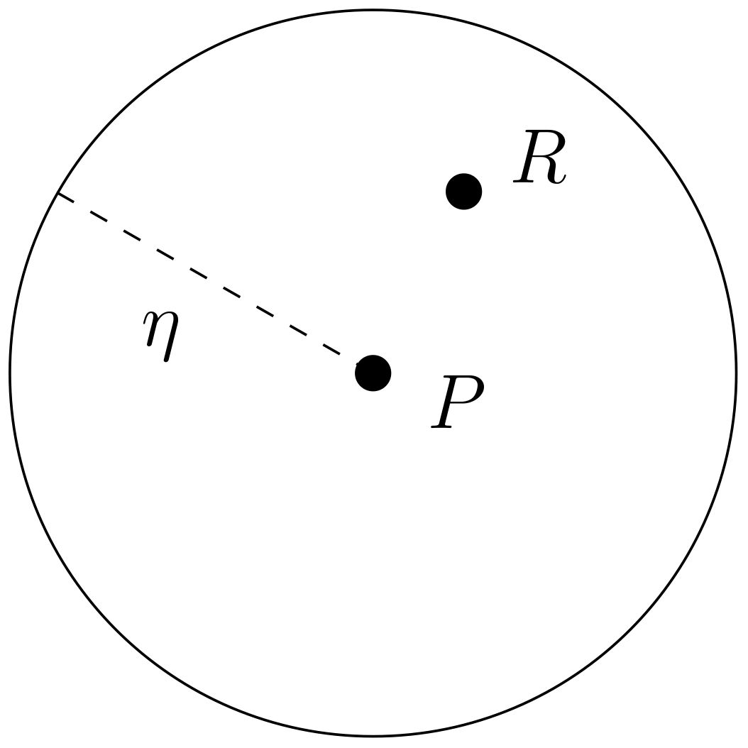
Figure 1. Adapted from Hansen and Sargent (2011) (Figure 1.7.1). Set of nearby models, representing the “real world”, for which the decision rule will work well using the perceived model. R and P stand for real and perceived, respectively and η is the maximum distance between the two models representing the maximum scientific uncertainty accepted by managers.

The analysis reveals that when managers are concerned about scientific uncertainty, they know that a fraction of the volatility observed in the data is generated by the observer’s ignorance. For the sake of simplicity, the source of uncertainty in our framework is considered to affect recruitment, which is characterized as a persistence model affected by shocks. In this context, managers infer that the real model –which is generating the perceived recruitment shocks– is more persistent than the perceived model. As a result, robust HCRs have to be designed assuming a more persistent fishery dynamics process than the one perceived in the data. In particular, our analysis shows that a robust HCR always has a higher limit reference point for the precautionary biomass. Thus, for the range of biomass between the precautionary and the target values, the linear relationship established by the standard HCR becomes steeper in the robust context than in the non-robust setting.

Finally, we show that HCRs that use half of the biomass level associated with MSY (0.5B_MSY) as the limit reference point for the precautionary biomass are consistent with our theoretical results. In this sense, our results can be said to be aligned with practices such as those implemented by the Australian and New Zealand fisheries authorities (Rayns, 2007; New Zealand Ministry of Fisheries, 2008) or with the proposal by Froese et al. (2011) for European fisheries management.

The rest of the paper is organized as follows: Section 2 describes the assumptions under the model and the characterization of robust HCRs. Section 3 shows the theoretical findings of the analysis and derives a rule of thumb for fixing critical values for the biomass. Section 4 concludes by discussing the results.

2 Methods

2.1 Harvesting control rules and limit reference points

Determining optimal fishing mortality may not be sufficiently helpful from an operational viewpoint. Different management approaches, including what is politically feasible, lead to fisheries management being implemented through different tools (e.g., total allowable catch (TAC) limits, limits on the amount of fishing effort, restrictions on the gear, seasonal closures), sometimes in a combined way and with different degrees of success (Da-Rocha and Gutiérrez, 2012; Selig et al., 2017).

A well-managed fishery requires the design of explicit harvest strategies that indicate how much catch should be attempted to be harvested under what circumstances (Hilborn and Walters, 1992, Chapter 15). In practice, simple rules, known as harvest control rules (HCRs), are used by many fisheries managers to set a target level of fishing mortality. However, any specific design of HCR depends on the quantity and quality of data available for the fishery (Smith et al., 2009; Punt, 2010). For those stocks with the highest quality information available, a model-based HCR design may be appropriate. In these cases, as Eikeset et al. (2013) point out, an HCR can be understood as an algorithm that relates state variables that show the biological information of the fishery (e.g., biomass, spawning biomass, etc.) to the control variables of the fishery that reflect the management information (e.g., fishing mortality, effort, catches, etc.). In those cases with poor or limited data, “empirical” HCR can be proposed (Punt, 2010). For instance, when targets and limits are based on historical standardized catch rate, a cpue-based HCR is more appropriate (Little et al., 2011; Jardim et al., 2015). This type of HCR has proved to be particularly effective in mixed and multi-specific fisheries (Canales et al., 2024).

HCRs take different forms in different settings in real practice (Kvamsdal et al., 2016; Free et al., 2023). For the purpose of this study, we focus on standard model-based HCRs that advise on fishing mortality that targets MSY (F_MSY) by considering precautionary biomass thresholds B_lim and B_trigger. The threshold B_lim represents the point below which it is believed that the reproductive capacity of the stock may be at risk, so the HCR prohibits fishing when biomass drops below it (i.e., fishing mortality is set to zero). In this sense B_lim can be understood as a precautionary threshold that can be imposed even if there is not complete information on the reproductive capacity of the stock below that threshold. The threshold B_trigger represents the lower bound compatible with a given biomass target and the HCR consists of setting a constant fishing mortality consistent with that biomass level whenever the biomass is above that threshold. When the biomass is in the range (B_lim, B_trigger), the HCR establishes a linear relationship between fishing mortality and biomass. Figure 2 shows this type of HCR, which is referred to as “protective” by Mackinson et al. (2018) regarding the North Sea multi-annual plan (European Commission, 2016). Note that when targets are given by fisheries policy makers, a characterization of HCR consists in selecting appropriate B_lim according to some criteria.

Figure 2

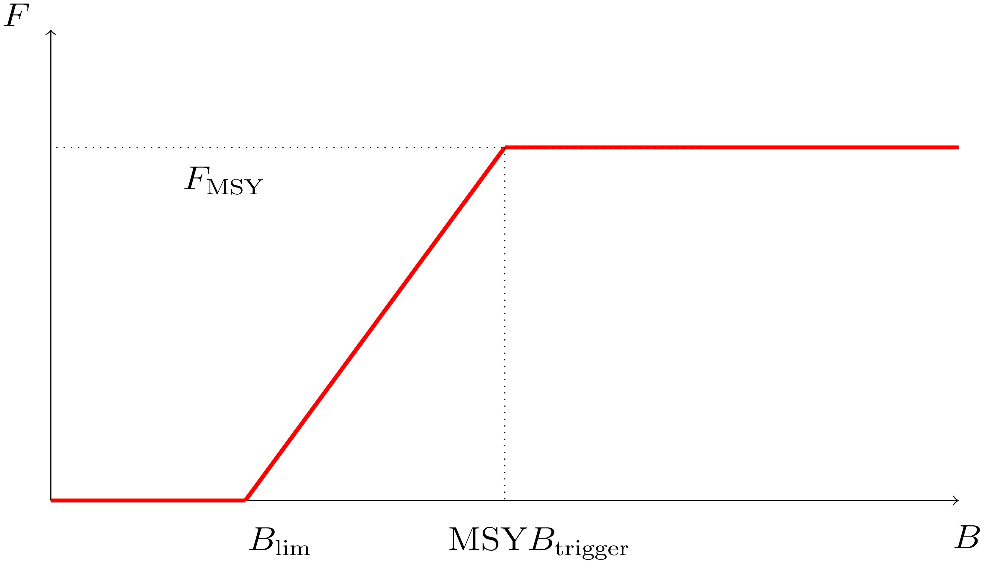
Figure 2. A “protective” HCR based on biomass thresholds B_lim and B_trigger with MSY as the target (Mackinson et al., 2018, Figure 4B).

In actual practice, the concept of precautionary biomass is more complex. For instance, the Harvest Strategy Standard for New Zealand Fisheries establishes two types of limit reference points associated with different management actions called”soft limits” and “hard limits” (Mace et al., 2013). The soft limit is a biomass level below which a stock must be subjected to a formal, time-constrained rebuilding plan to rebuild it back to the B_MSY (usually 1/2 B_MSY or 20% of the biomass in the absence of fishing -B₀ o B_F=0 -, whichever is higher). The hard limit is a biomass level below which all fishing activity on the stock in question should cease (usually 1/4 B_MSY or 10% B₀, whichever is higher). There are variations on this theme. For the US National 1 Standard Guidelines, for example, a minimum stock size threshold (MSST, usually equivalent to about 1/2 B_MSY) is specified below which a similar type of formal, time-constrained rebuilding plan is required to rebuild the stock back to B_MSY. However, the guidelines do not specify a biomass limit below which all fishing for a stock must cease, although some US jurisdictions or individual US fisheries do so (US National Marine Fisheries Service, 2016). The Australian Harvest Strategy Policy (DAW, 2018) sets B_lim at 0.2B₀ which, based on their other definitions, would be consistent with 1/2 B_MSY. When this point is reached, all directed fisheries for the stock in question should be closed, but bycatch fisheries may remain open within limits.

In any case, the design of any HCR also requires a relatively high level of data and knowledge of the dynamics of the stocks concerned. In the type of HCR referred to here, it is necessary to know the values of the target reference points (e.g., those associated with MSY) and the biomass thresholds, B_trigger and B_lim. To estimate these values accurately, complete knowledge of the biological, economic, and ecologic models behind the stock population dynamics is needed. It is not always possible to apply the HCR because of the lack of information. For example, in 2005, it was only possible to use this type of HCR on 22 of the 80 species managed by the Pacific Fishery Management Council (Punt and Donovan, 2007).

An additional problem is that in most cases, the design of HCRs does not explicitly include a way to deal with uncertainty (Punt and Donovan, 2007; Deroba and Bence, 2008). In the case of European fisheries stocks, when the data and knowledge requirements are not fulfilled, ICES sometimes advises a lower fishing mortality than F_MSY even when the stock is in good conditions; for instance, F_0.1, instead of F_MSY, which is the mortality rate where the yield per recruit slope is 10% of the maximum yield per recruit slope.

2.2 The population model

We build up the population model as in Da-Rocha and Mato-Amboage (2016), where a stochastic version of the fishery of Hannesson (1975) is considered with two age classes: juveniles and adults. Let N_t,1, and N_t,2 be the populations of juveniles and adults in period t, respectively. Each year, t, a stochastic exogenous number of juvenile fish are born, N_t,1 = exp(z_t), where z_t is a random variable that determines the recruitment of the fishery. This is the only source of uncertainty affecting the model and it is perceived by the managers as following an AR(1) process:

$\begin{array}{ll}{z}_{t+1}=\rho z_t+{\widetilde{ϵ}}_{t+1},& (1)\end{array}$

where ${\widetilde{ϵ}}_{t+1}$ is a Gaussian i.i.d. process with zero mean and variance ${\sigma }_{ϵ}^2$, and $\left|\rho \right|\in [0,1)$ is the autocorrelation coefficient.

Managers see this perceived model as an approximation to the real model, representing the “real world”. Following Hansen and Sargent (2011), this scientific uncertainty is represented with a set of alternative models of the form

$\begin{array}{ll}{z}_{t+1}=\rho z_t+{ϵ}_{t+1}+{\omega }_{t+1},& (2)\end{array}$

where ${ϵ}_{t+1}$ is another Gaussian i.i.d. process with zero mean and variance ${\sigma }_{ϵ}^2$, and ${\omega }_{t+1}$ is a vector of perturbations in the mean of ${\widetilde{ϵ}}_{t+1}$, that can feed back into the history of the state, $z$. Note that since process represented in Equation 2 is the model that generates the data, it is as though the errors ${\widetilde{ϵ}}_{t+1}$in the perceived model (1) were conditionally distributed as $\mathcal{N}({\omega }_{t+1},{\sigma }_{ϵ}^2)$ rather than as $\mathcal{N}(0,{\sigma }_{ϵ}^2)$. Moreover, it is also important to highlight that perturbations ${\omega }_{t+1}$ affect the real persistence of recruitment. Since ${\omega }_{t+1}$ feeds back into the history of the state, $z$, parameter $\rho$ does not represent persistence in the real model (2). We show bellow what this real persistence is when managers select optimal HCRs.

The dynamics of the adult age group is then given by $N_{t+1,2}=N_{t,1}{e}^{-F_t-m},$, where $F_t$ represents the fishing mortality applied in period t and m is the natural mortality rate, which for the sake of simplicity is assumed to be constant over time. Finally, for this proof-of concept article we assume, as Da-Rocha and Mato-Amboage (2016), that the spawning stock biomass of the fishery is defined as $B_t=\text{ln }{N}_{t,2}$. This relation implies that the spawning stock biomass is an increasing function of the number of adults in the population and that only a non-constant fraction of adults are spawners¹.

This population representation enables policymakers’ constraints to be modeled as a linear-quadratic problem, which is essential to apply the robust control theory (Hansen and Sargent, 2011).

2.3 Robust precautionary HCRs

Uncertainty is modeled following the multiplier preference approach based on the robust control theory proposed by Hansen and Sargent (Hansen and Sargent, 2001, 2011). Under this framework, optimal (robust) policies are selected among all possible distributions consistent with what is known and observed, by adding a penalty term that is inversely related to the distance of any given distribution from the best guess.

We start by assuming that fishery managers want to design a robust precautionary HCR that linearly relates fishing mortality and biomass so that exogenous targets $(B_{tar},F_{tar})$ are achieved while avoiding the risk of the stock falling below level B which would result in the fishery being considered as no longer sustainable from the biological viewpoint. Note that we are assuming that $B_{tar}$ and $F_{tar}$ are exogenously given by the managers². A typical ICES HCR considers $B_{tar}=\text{ MSY }{B}_{trigger}$ and $F_{tar}=F_{\text{MSY}}$ (Mackinson et al., 2018).

The objective function of managers is characterized in terms of distances of fishing mortality and biomass from their respective target points as in Da-Rocha and Mato-Amboage (2016). They aim to stabilize the resource around the desired points. This idea is formalized with a loss function that represents the net present weighted sum of the squared distance of fishing mortality, $F_t$, and biomass, $B_t$, from their respective targets

$\begin{array}{ll}{E}_0\sum _{t=0}^{\infty }{\beta }^{t+1}[{(F_t-F_{tar})}^2+\text{λ}{(B_t-B_{tar})}^2],& (3)\end{array}$

where 0 < β < 1 represents the subjective discount rate, E₀ is the mathematical expectation conditioned on the information available at the time of decision-making and λ is a parameter that represents the weight of biomass deviation relative to fishing mortality deviation. There are three noteworthy remarks regarding the managers’ loss function (3): First, F is, by definition, a variation rate (mortality rate), and its deviation from its target is also a rate. In addition, the deviation of the B from its target must also be seen also as a variation rate since both variables are defined in logarithms. Hence, the two sums of the loss functions are ratios with no measurement units. Second, it penalizes both deviations above or below the desired values (hence the square of the distance). Third, it considers the dynamic nature of the resource, enabling long-run deviations to be offset by more minor deviations in the short run. How much present deviations can offset future deviation depends on the discount factor, β: Larger discount factors mean small discount rates, that is managers care as much about future changes as if they occurred in the current year³.

An HCR can be understood as the result of minimizing the loss function (3), taking into account the population model. This interpretation means that an HCR is characterized by the parameter λ. Note that with λ = 0 the rule is independent of the biomass, and the instrument is constant over different biomass levels. With λ approaching infinity, the rule is (equivalently) linear in the biomass level, and a bang-bang or most rapid approach path solution emerges. A positive, finite lambda dictates a trade-off between fishing mortality and biomass and may be associated with a positive $B_{\text{lim}}$. Figure 3 illustrates these cases, which shows are somewhat reminiscent of classical thinking as embodied by (Hilborn and Walters, 1992, Chapter 15).

Figure 3

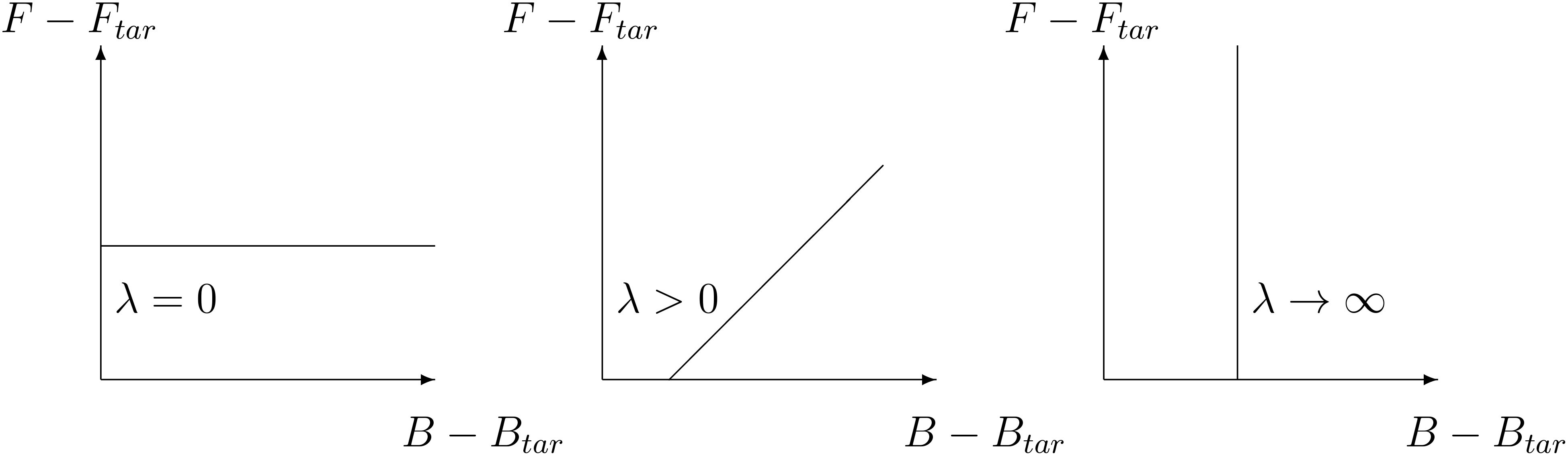
Figure 3. λ = 0 is associated with a constant effort HCR; λ > 0 is associated with a biomass-based HCR; λ → ∞ is associated with a constant or fixed escapement rule.

An HCR that follows the precautionary principle is sought here, so the rule needs to ensure at most a v% probability of the biomass falling below the limit point, B; that is, the HCR has to satisfy the requirement that

$\begin{array}{ll}Pr(B\le \underset{\_}{\text{B}})\le v,& (4)\end{array}$

where v is given by the managers. Equation 4 specifies a precautionary HCR which guarantees that the stock is above the limit point $\underset{\_}{\text{B}}$ with at least a 1 − v% probability (e.g., v = 0.05 for ICES advice).

In addition, managers know that the perceived model (1) is an approximation of the real model (2), so they are aware of the dynamic misspecification of the model (the scientific uncertainty). Therefore a scientific uncertainty level η is considered, i.e.

$\begin{array}{ll}{E}_0\sum _{t=0}^{\infty }{\beta }^{t+1}{\omega }_{t+1}^2\le \eta .& (5)\end{array}$

The left-hand side of Equation 5, $E_0{\sum }_{t=0}^{\infty }{\beta }^{t+1}{\omega }_{t+1}^2$, is an intertemporal measure of the size of model misspecification called conditional relative entropy. This constraint is used to measure the statistical discrepancy between the perceived model (1) and the real model (2), which differ only in the ω term [see Hansen and Sargent (2011)]. Therefore, Equation 5 expresses the idea that managers know that the real model can be any nearby model around the perceived model (see Figure 1). The parameter η measures the set of models surrounding the perceived model for which managers think the decision rule will work well. More significant scientific uncertainty implies a more extensive set of alternative models that may represent the “real world” to be compared with the perceived model. So in this context, η can be understood as a measure of scientific uncertainty accepted by managers. Formally, the conditional relative entropy is constrained to be lower than or equal to an exogenous scientific uncertainty level η which the managers provide.

(Hansen and Sargent 2011, chapter 9) propose using Bayesian detection error probability to estimate η when guiding the choice of the set of models against which the perceived model is compared. This approach assumes that the models on and inside the ball In Figure 1 are difficult to distinguish statistically from the real model with the amount of data at hand. In essence, it takes a neutral stance on whether the true data-generating process is represented by the perceived model or by the worst-case model (at the boundary of the ball). The method involves calculating the likelihood ratio tests to choose between these two models under both hypotheses, bases on in-sample fit, for a sample of a given size. Then a probability of a detection error is calculated on the basis of a large number of simulations by giving equal probability to the two models of being the true model.⁴ When the model assumes no robustness (maximum η), the detection error probability es 50%. Hansen and Sargent (2011) suggest choosing η such that the range for the detection error range is between 10% and 20%. Sample size also plays an important role. The larger the available sample is, the lower η is chosen because the uncertainty is less of a concern.

Considering all these specifications, in looking for a robust precautionary HCR, the managers’ problem consists of minimizing the loss function expressed in Equation 3, taking into account the population model and the precautionary and misspecification side constraints Equations 4, 5, respectively).

Technically, the robust precautionary HCR is characterized in two steps. First, for a given HCR (a given λ) and an admitted uncertainty level η, managers seek to maximize their intertemporal target gap while a hypothetical malevolent nature minimizes that same target by selecting the worst perturbation process, given the population dynamics. Formally, the following extremization problem is solved:

$\begin{array}{ll}\begin{array}{l}\underset{{\left\{F_t,B_{t+1}\right\}}_{t=0}^{\infty }}{\max }\underset{{\left\{{\omega }_{t+1}\right\}}_{t=0}^{\infty }}{\min }{E}_0\sum _{t=0}^{\infty }{\beta }^t\left\{-{(F_t-F_{tar})}^2-\text{λ}{(B_t-B_{tar})}^2+\beta \theta {\omega }_{t+1}^2\right\},\\ \begin{array}{cc}& s.t.\{\begin{array}{l}{B}_{t+1}=z_t-F_t-m,\hfill \\ z_{t+1}=\rho z_t+{ϵ}_{t+1}+{\omega }_{t+1}.\hfill \end{array}\end{array}\end{array}& (6)\end{array}$

where the multiplier θ represents the penalty for deviating from the real model in the function to be optimized. Note that since the problem seeks to minimize of the perturbation ω, a very low θ allows the nature to wreak havoc, while θ → ∞ corresponds to a zero penalty for the deviation.

Second, given the target paths solutions from the extremization problem (Equation 6), the HCR, λ, and the multiplier θ associated with the scientific uncertainty level, η, that satisfy the precautionary and misspecification constraints (Equations 4, 5, retrospectively) are found. To this respect, it should be noted that since the function to optimize is monotonous and concave in η, there is a negative bijective function from η to the multiplier θ (Giordani and Söderlind, 2004).

Appendix A.1 proves that for a given scientific uncertainty level η and a precautionary probability of biomass falling below the limit point, v, the robust precautionary HCR is given by

$\begin{array}{ll}\text{λ}=\frac{1}{\beta }\left[\frac{{\sigma }_{ϵ}{\text{erf}}^{-1}(2v-1)\sqrt{2}}{(\underset{\_}{\text{B}}-B_{tar}){(1-{\widehat{\rho }}^2)}^{1/2}}-1\right],& (7)\end{array}$

where erf is the Gaussian error function and $\widehat{\rho }$ is given by

$\begin{array}{ll}\eta =\frac{\beta }{1-\beta }\frac{{(\widehat{\rho }-\rho )}^2{\sigma }_{ϵ}^2}{(1-{\widehat{\rho }}^2)}.& (8)\end{array}$

Parameter $\widehat{\rho }$ can be interpreted as the actual persistence of the real model. This parameter is unknown to managers but is endogenously determined by Equation 8 for a given scientific uncertainty. Two facts that emerge from Equation 8 are worth noting: On the one hand, if managers are not concerned about scientific uncertainty ($\eta \to 0$), then $\widehat{\rho }=\rho$. However, when managers are highly concerned about scientific uncertainty ($\eta \to \infty$), $\widehat{\rho }>\rho$ meaning that the (inferred) real model is more persistent than the perceived one. On the other hand, even for uncorrelated perceived processes ($\rho =0$), a robust HCR would have to consider the existence of some persistence, i.e. ${\widehat{\rho }}^2=\frac{\eta }{\left(\frac{\beta }{1-\beta }\right){\sigma }_{ϵ}^2+\eta }>0$.

Finally, the complete characterization of the robust HCRs given by Equations 7, 8 shows unambiguously that the more significant the scientific uncertainty (η) is, the larger ${\widehat{\rho }}^2$ and λ are.

3 Results

3.1 Theoretical findings

Two theoretical conclusions can be highlighted from the characterization of robust precautionary HCRs (Equations 7, 8). First, an HCR of keeping fishing mortality constant at the target level cannot be a precautionary robust rule.

Proposition 1. A constant effort rule, $F_t=F_{tar}$ is not a robust precautionary HCR. Therefore, a robust limit reference point for biomass is greater than zero.

Proof: See Appendix A.2

Under scientific uncertainty, it can be inferred that the real process is correlated, even when the stochastic process obtained from the perceived model is not. Robustness implies the use of biomass-based HCRs, λ > 0 (see a numerical example in Da-Rocha and Mato-Amboage (2016)).

The logic behind the result that a constant effort HCR is not robust under scientific uncertainty can be illustrated with the following reasoning. Suppose that a naive manager considers both that the perceived model (1) is the one that generates the data (but it is not) and the process is perceived as uncorrelated, $\rho =0$. Under this assumption, a constant effort HCR, ${\text{λ}}^{NR}=0$, is expected to generate a variance ${\tilde{\sigma }}_{ϵ}=\frac{(\underset{\_}{\text{B}}-B_{tar})}{{\text{erf}}^{-1}(2v-1)\sqrt{2}}$ (from Equation 7 when $\text{λ}=0$ and $\rho =0$). This result means that the expected biomass volatility -based on naive expectations- is ${\sigma }_B^2={\tilde{\sigma }}_{ϵ}^2$. However, data is generated not by the perceived model (1) but by the real model (2), which includes the perturbation $w_{t+1}$. Therefore, the volatility of the biomass is actually given by ${\sigma }_B^2=\frac{{\sigma }_{ϵ}^2}{1-{\widehat{\rho }}^2}$.⁵

Managers concerned with robustness seek reliable HCR for all close real models (2) in the set shown in Figure 1. This is equivalent to designing an HCR that takes into account that $\widehat{\rho }>\rho =0$. This robust HCR is given by Equation 7 and for an uncorrelated process is ${\text{λ}}^R=\frac{1}{\beta }\left[\frac{1}{{(1-{\widehat{\rho }}^2)}^{1/2}}-1\right]>0$. It generates a risk measure of

$\begin{array}{ll}Pr(B\le \underset{\_}{\text{B}})=\frac{1}{2}[1+\text{erf}((1+{\text{λ}}^R\beta ){(1-{\widehat{\rho }}^2)}^{1/2}\text{er}{\text{f}}^{-1}(2v-1))].& (9)\end{array}$

Figure 4 shows how naive HCR performance deteriorates more quickly than robust HCR rules as scientific uncertainty (the correlation generated by the perturbation process, $\widehat{\rho }$) increases. When the naive constant effort rule, ${\text{λ}}^{NR}=0$, is applied the precautionary constraint is violated, i.e.

Figure 4

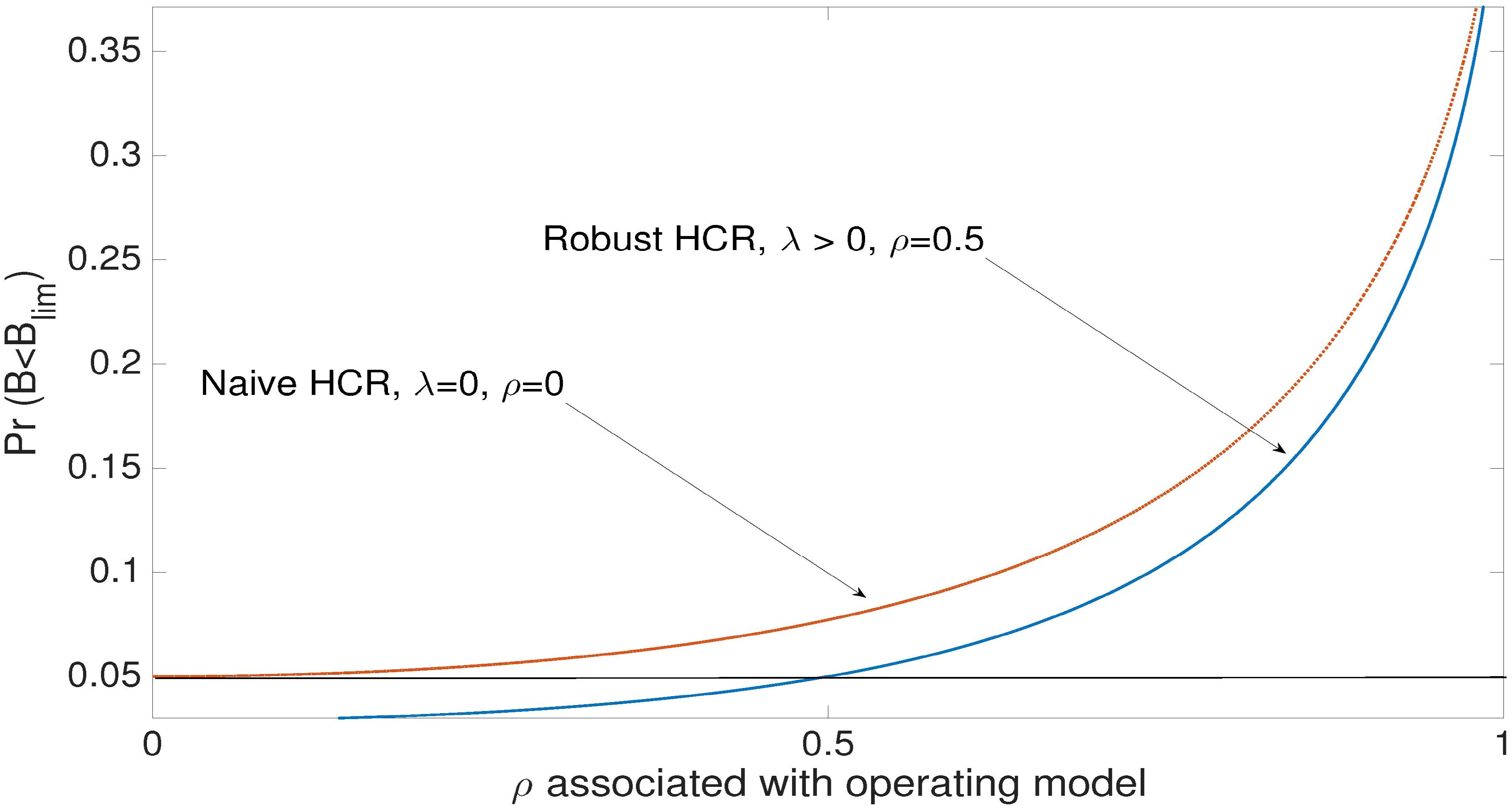
Figure 4. Risk of biomass dropping below $\underset{\_}{\text{B}}$ for a naive HCR, λ = 0 (Equation 10) and a robust HCR, λ > 0 (Equation 9). The robust HCR was designed by assuming $\widehat{\rho }$ to be 0.5. Notice that when the correlation generated by the real model is 0.5 the probability of the biomass dropping below $\underset{\_}{\text{B}}$ is exactly v = 0.05.

$\begin{array}{ll}Pr(B\le \underset{\_}{\text{B}})=\frac{1}{2}[1+\text{erf}({(1-{\widehat{\rho }}^2)}^{1/2}{\text{erf}}^{-1}(2v-1))]>v.& (10)\end{array}$

In general, HCR reduces precautionary levels when the perceived model is correct. However, the performance becomes more precautionary as scientific uncertainty increases.

Second, how much faster fishing mortality is reduced when a stock is assessed to be below the target biomass depends on the level of scientific uncertainty. Our results show that for the same uncertainty concern and precautionary criteria (given by $\eta$ and $v$), a robust HCR selects a higher biomass limit reference point ($B_{\text{lim}}$) than non-robust HCR. Figure 5 illustrates this result showing that $B_{\text{lim}}^R>B_{\text{lim}}^{NR}$. Given this, the linear relationship between fishing mortality and biomass in the range $(B_{\text{lim}},B_{\text{tar}})$ becomes steeper with $\text{λ}(\rho )>\text{λ}(\widehat{\rho })$. Proposition 2 establishes these results formally.

Figure 5

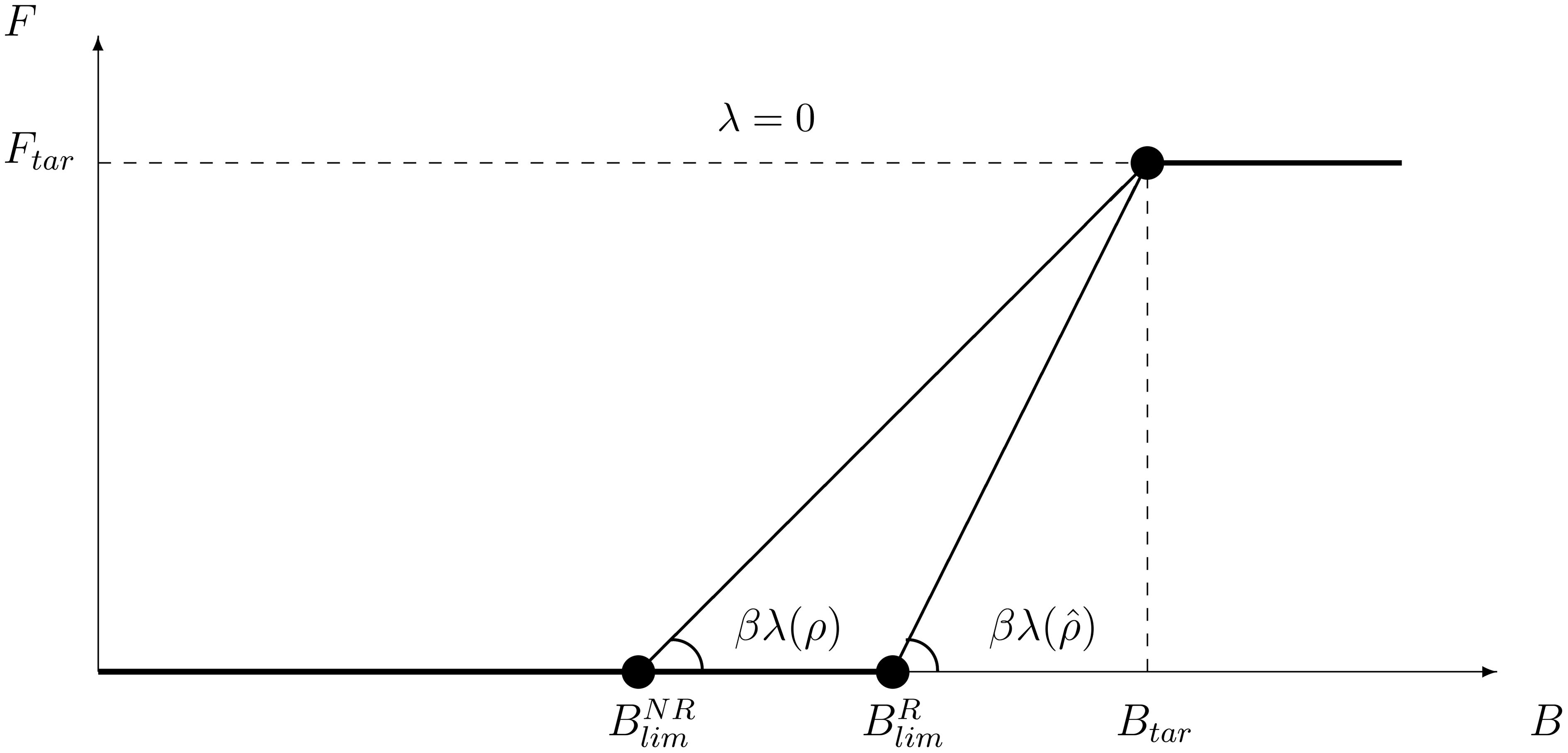
Figure 5. Robust HCR versus non-robust HCR. Robust design of HCR leads to a higher limit reference point for the biomass. $B_{\text{lim}}^{NR}$ and $B_{\text{lim}}^R$ stand for non-robust and robust biomass limit reference points, respectively.

Proposition 2. Greater scientific uncertainty levels imply: i) a steeper relationship between biomass and robust fishing mortality in the robust HCR, and ii) a higher limit reference point for biomass, which is given by $B_{lim}=B_{tar}-F_{tar}/\beta \text{λ}(\widehat{\rho })$.

Proof: See Appendix A.3.

3.2 A robust rule of thumb for HCR

According to our modeling, characterizing the robust precautionary HCR for a particular stock would require time series data to compute ${\sigma }_{ϵ}$, $\rho$, and $\underset{\_}{\text{B}}$. However, if the idea is only to explore the impact of scientific uncertainty –for the given levels of v– there is no need to compute these statistics.

To see this more clearly, assume that the stock has been assessed as above $B_{\text{trigger}}$, and the ICES MSY (constant effort) advice rule has been applied. In that case, (see Appendix A.4), the robust precautionary HCR has to satisfy the requirement that

$$\beta \text{λ}={\left(\frac{1-{\rho }^2}{1-{\widehat{\rho }}^2}\right)}^{1/2}-1=\frac{\widehat{\sigma }-\sigma }{\sigma },$$

where $\sigma$ and $\widehat{\sigma }$ represent the standard deviation of the recruitment process in the perceived model (1) and in the real model (2), respectively. This result means that robustness is proportional to the difference between the standard deviation of the perceived and the real models.

Following the three-sigma rule, $\widehat{\sigma }=3\sigma$, which guarantees that 99.7% of random events lie around the mean of its normal distribution (see Pukelsheim (1994)), the robust HCR is to set βλ as 2. This result implies that whenever the biomass is above the limit reference point for the biomass, $B_{\text{lim}}$, the robust HCR sets fishing mortality such that its deviation from the target is twice the deviation of the biomass from its target. Moreover, the robust HCR also endogenously determines the biomass reference point as half of the biomass target, i.e., $B_{\text{lim}}=0.5B_{\text{MSY}}$.

In short, the limit reference point used by Australian and New Zealand fisheries authorities (New Zealand Ministry of Fisheries, 2008; Sainsbury, 2008) and proposed by Froese et al. (2011) for European fisheries management is the endogenous robust limit point associated with a robust HCR where fishing mortality deviation is twice the biomass deviation when a stock is assessed using a three-sigma rule.

4 Discussion and conclusions

Marine resource management procedures that take account for uncertainty include specification of the data to be collected and how these data will be used to provide management advice that incorporates feedback mechanism in the form of decision rules to HCRs (Punt and Donovan, 2007). This paper shows that scientific uncertainty can be treated analytically using the robust control theory proposed by Hansen and Sargent (Hansen and Sargent, 2001, 2011). In particular, robust model-based HCRs are theoretically characterized in closed form using this approach. This result is a novelty with respect to other papers that also study robust control in natural resource management (Vardas and Xepapadeas, 2010; Athanassoglou and Xepapadeas, 2012; Xepapadeas and Roseta-Palma, 2013).

This theoretical characterization of robust HCRs allows establishing two novel points to be made from a fisheries management perspective. First, it can be stated theoretically that constant HCRs are not robust under scientific uncertainty. This result provides theoretical support for approaches suggesting that, in the presence of uncertainty, biomass-based threshold HCRs, which indicate that fishing mortality should decrease with biomass, are more appropriate than constant fishing mortality HCRs (Deroba and Bence, 2008; Punt, 2010). Second, robust HCRs set higher biomass precautionary reference points than those of non-robust HCRs. Moreover, these precautionary levels are defined in terms of target reference points [as in Froese et al. (2011)]. These results are aligned with the idea that sources of uncertainty can be reduced by defining intervals around the limit reference points (Rindorf et al., 2016; Da-Rocha et al., 2017; Rindorf et al., 2017a, b) or by choosing appropriate methods for estimating them (van Deurs et al., 2021; Bi et al., 2023).

This research also show that these theoretical findings can be easily implemented by designing HCRs that use 0.5B_MSY as the limit reference point for biomass. In this sense, our results can be said to be aligned with real practices. The Australian Harvest Strategy Policy (DAW, 2018) identifies 20% of the biomass in absence of fishing (0.2B₀) as the standard limit reference point because it is considered a suitable proxy that avoids recruitment overfishing for productive stocks (Sainsbury, 2008). For less productive stocks, more conservative limit reference points are proposed (e.g. 0.3B₀). Additionally, the Australian Harvest Strategy considers that if B_MSY can be reliably estimated and it is above 0.4B₀ then 0.5B_MSY is an appropriate alternative as a limit reference point (Rayns, 2007). New Zealand uses 0.5B_MSY as a limit below which a formal rebuilding plan is required (New Zealand Ministry of Fisheries, 2008). Froese et al. (2011) propose using this limit reference point to design HCR to manage European fisheries. More recently, Froese et al. (2018) use this reference to asses European stocks and found 51% of them to be outside safe biological limits.

In this regard, it is worth mentioning that it has been common practice in the International Council for the Exploration of the Sea (ICES) in the last few years to set management reference points based on a deterministic equilibrium relationship between yield, fishing mortality, and biomass (ICES, 2017). In particular, for stocks for which there is no appropriate population information, the deterministic version of the surplus production Schaefer model (Schaefer, 1954) is used and in most cases 1/3B_MSY set as a proxy for $B_{\lim }$ This deterministic approach is no appropriate because, in general terms, deterministic reference points overestimate fishing mortality and the biomass required to support MSY. For example, the US, Australia and New Zealand all have the default assumption that $B_{\text{MSY}}=0.4B_0$, which is way higher than the deterministic B_MSY in most cases. In any case, notice that this selection is not incompatible with our results. We find that with uncertainty, the level of precautionary biomass (below which fishing is banned) should be higher than in deterministic cases. In this context, it is worth studying whether it is advisable to increase $B_{\text{lim}}$ from 1/3B_MSY to 0.5B_MSY.

On the other hand, ICES has recently started using the SPiCT model for their MSY advice. SPiCT is a surplus production model that takes uncertainty in catches and biomass indexes into account (Pedersen and Berg, 2017). This framework enables precautionary limits to fishing mortality $(F_{p-05})$ to be set such that the probability of the predicted biomass being below an agreed lower limit $(B_{\text{lim}})$ is 5% or less (Rindorf et al., 2016). From this perspective, our characterization of the precautionary biomass associated with the robust HCR ($B_{\text{lim}}^R$ in Figure 5) is a concept similar to the predicted biomass implied for the precautionary fishing mortality $(F_{p-05})$ in Rindorf et al. (2016). The novelty of our result is it supports this idea for stocks whose population can be described in a very simple way from age cohorts.

From the point of view of the stock modeling, it should be emphasized that in this study it has been set up in the simplest way possible. In particular, it has been assumed that the stock is divided into two age groups (juveniles and adults) without considering the existence of a plus group and the spawning stock biomass follows a logarithmic relationship with the adult population. Furthermore, the only source of uncertainty considered is recruitment, which is assumed to be autocorrected to order 1. All these simplifications may seem far removed from the reality observed in the population dynamics of most fish stocks. However, this simplified modeling is useful (and necessary) to obtain analytical solutions that help interpret the results in simple scenarios. Application of the model to specific populations would require adaptation to account for their intrinsic biological characteristics.

The simplification of the biological model to a form with only one source of uncertainty suggests that this study is a kind of proof of concept for a single source of uncertainty. However, one of the attractions of the methodology used in this study is that the class of disturbances used to capture uncertainty may be more general than the simplicity of the model analyzed apparently shows. With Hansen and Sargent (2011) approach, the uncertainty considered may include unknown parameter values and misspecfication of higher moments of the error distribution as long as the decision maker’s objective function is quadratic and his approximating model is linear with Gaussian errors (see chapters 1.13, 3 and 7). Even more structured kinds of uncertainty can be accommodated by slightly reinterpreting the decision maker’s objective function (see chapter 19). In this sense, this approach can be extended to all the sources of uncertainty classified by Francis and Shotton (1997), i.e., observation, model structure, process error, and implementation errors. Therefore, our findings can be applied in case studies that use the simulation modeling approach to assess different management strategies (MSE) under various sources of uncertainty. Even in those fisheries with poor data, the proposed methodology can be used to design robust HCR that link abundance indices such as CPUE or survey data with catch limits.

This study focuses on HCRs that aim to maintain stock biomass at levels consistent with MSY, relying on a limited number of biological reference points ($F_{tar}$, $B_{tar}$ and $B_{lim}$), where ed as a biomass limit reference point that indicates the closed/open status of the stock to the fishing activity. This simplification can be seen as a limitation because it does not take into account that fisheries management may have multiple objectives (maximizing catch, minimizing risk to the resource, and maximizing industrial stability) that may conflict with each other. To mitigate these possible conflicts in the presence of uncertainty, several types of measures have been recommended; among others, the definition of optimal HCRs based on a larger number of biological reference points (Yagi and Yamakawa, 2020), the evaluation of the theoretical and applied impact of spatio-temporal measures (Da-Rocha et al., 2012; DAW, 2018), the valuation of fishery resources with non-constant discount factors (Da-Rocha et al., 2016). The robustness of such solutions could also be evaluated in the context of robust control theory, extending the applicability to actual practice.

Data availability statement

The original contributions presented in the study are included in the article/supplementary material. Further inquiries can be directed to the corresponding author.

Author contributions

J-MD-R: Writing – review & editing, Writing – original draft, Visualization, Validation, Supervision, Software, Resources, Project administration, Methodology, Investigation, Funding acquisition, Formal analysis, Data curation, Conceptualization. JG-C: Writing – review & editing, Writing – original draft, Visualization, Validation, Supervision, Software, Resources, Project administration, Methodology, Investigation, Funding acquisition, Formal analysis, Data curation, Conceptualization. M-JG: Writing – review & editing, Writing – original draft, Visualization, Validation, Supervision, Software, Resources, Project administration, Methodology, Investigation, Funding acquisition, Formal analysis, Data curation, Conceptualization.

Funding

The author(s) declare financial support was received for the research, authorship, and/or publication of this article. J-MD-R and JG-C gratefully acknowledge financial support from Xunta de Galicia (ED431B 2022/03). M-JG also acknowledges financial support from the Basque Government (BiRTE IT-1461-22) and the University of the Basque Country (PES20/44).

Acknowledgments

The authors thank Andre Punt, Pamela Mace and Gorka Merino who have considerably improved the article.

Conflict of interest

The authors declare that the research was conducted in the absence of any commercial or financial relationships that could be construed as a potential conflict of interest.

Publisher’s note

All claims expressed in this article are solely those of the authors and do not necessarily represent those of their affiliated organizations, or those of the publisher, the editors and the reviewers. Any product that may be evaluated in this article, or claim that may be made by its manufacturer, is not guaranteed or endorsed by the publisher.

Footnotes

1. ^ The application of this model to a specific stock would require empirical testing of the relationship between spawning stock biomass and the adult population and even taking into account other variables that accurately measure reproductive potential (Kell et al., 2016).
2. ^ In real fisheries, however, these variables are selected endogenously according to management criteria that typically allow for long-term sustainable and efficient exploitation of the stocks (Yagi and Yamakawa, 2020).
3. ^ Discount is frequently introduced into fishery economics using the discount rate, r, instead of a discount factor, β; the former is usually applied in continuous time frameworks, whereas the latter is more commonly used in discrete set ups. The inverse relationship between the two is given by $\beta ={(1+r)}^{-1}$, which is compressed between 0 and 1 (Da Rocha et al., 2010). There is even some literature in which discounting the future is included as a time-varying factor (Da-Rocha et al., 2016).
4. ^ Technically, the detection error probabilities can be calculated using program detection2.m in Matlab.
5. ^ When ${\widetilde{ϵ}}_{t+1}$ is perturbed, biomass evolves following $\text{Δ}{B}_{t+1}=\widehat{\rho }\text{Δ}{B}_t+\frac{1}{1+\beta \text{λ}}{ϵ}_t$. See Equation 17 in Appendix A.1.2 for further details.

References

Athanassoglou S., Xepapadeas A. (2012). Pollution control with uncertain stock dynamics: When and how to be precautious. J. Environ. Econ. Manage. 63, 304–320. doi: 10.1016/j.jeem.2011.11.001

Crossref Full Text | Google Scholar

Beddington J. R., Agnew D. J., Clark C. W. (2007). Current problems in the management of marine fisheries. Science 316, 1713–1716. doi: 10.1126/science.1137362

PubMed Abstract | Crossref Full Text | Google Scholar

Beverton R., Holt S. (1957). On the Dynamics of Exploited Fish Populations (London: Republished by Chapman and Hall), 19. doi: 10.1007/978-94-011-2106-4

Crossref Full Text | Google Scholar

Bi R., Collier C., Mann R., Mills K., Saba V., Wiedenmann J., et al. (2023). How consistent is the advice from stock assessments? Empirical estimates of inter-assessment bias and uncertainty for marine fish and invertebrate stocks. Fish Fish. 24, 126–141. doi: 10.1111/faf.12714

Crossref Full Text | Google Scholar

Canales C. M., Olea G., Jurado V., Espíondola M. (2024). Management Strategies Evaluation (MSE) in a mixed and multi-specific fishery based on indicator species: An example of small pelagic fish in Ecuador. Mar. Policy 162, 106044. doi: 10.1016/j.marpol.2024.106044

Crossref Full Text | Google Scholar

Da Rocha J. M., Cerviño S., Gutiérrez M. J. (2010). An endogenous bioeconomic optimization algorithm to evaluate recovery plans: an application to southern hake. ICES J. Mar. Sci. 67, 1957–1962. doi: 10.1093/icesjms/fsq116

Crossref Full Text | Google Scholar

Da-Rocha J., García-Cutrín J., Gutiérrez M., Jardim E. (2017). Endogenous fishing mortalities: A state-space bioeconomic model. ICES J. Mar. Sci. 74, 2437–2447. doi: 10.1093/icesjms/fsx067

Crossref Full Text | Google Scholar

Da-Rocha J., García-Cutrín J., Gutiérrez M., Touza J. (2016). Reconciling yield stability with international fisheries agencies precautionary preferences: The role of non constant discount factors in age structured models. Fish. Res. 173, 282–293. doi: 10.1016/j.fishres.2015.08.024

Crossref Full Text | Google Scholar

Da-Rocha J., Gutiérrez M. (2012). Endogenous fishery management in a stochastic model: why do fishery agencies use TACs along with fishing periods? Environ. Res. Econ. 53, 25–59. doi: 10.1007/s10640-012-9546-6

Crossref Full Text | Google Scholar

Da-Rocha J., Gutiérrez M., Antelo L. (2012). Pulse vs. optimal stationary fishing: The northern stock of hake. Fish. Res. 121-122, 51–62. doi: 10.1016/j.fishres.2012.01.009

Crossref Full Text | Google Scholar

Da-Rocha J., Mato-Amboage R. (2016). On the benefits of including age-structure in harvest control rules. Environ. Res. Econ. 64, 619–641. doi: 10.1007/s10640-015-9891-3

Crossref Full Text | Google Scholar

DAW (2018). Guidelines for the Implementation of the Commonwealth Fisheries Harvest Strategy Policy (Australian Government Department of Agriculture and Water Resources Canberra, Australia). Available online at: https://www.frdc.com.au/project/2016-234.

Google Scholar

Deroba J. J., Bence J. R. (2008). A review of harvest policies: Understanding relative performance of control rules. Fish. Res. 94, 210–223. doi: 10.1016/j.fishres.2008.01.003

Crossref Full Text | Google Scholar

Eikeset A. M., Richter A., Dankel D., Dunlop E., Heino M., Dieckmann U., et al. (2013). A bio-economic analysis of harvest control rules for the Northest Arctic cod fishery. Mar. Policiy 39, 172–181. doi: 10.1016/j.marpol.2012.10.020

Crossref Full Text | Google Scholar

EU (2013). Regulation (EU) no 1380/2013 of the European Parliament and of the Council of 11 December 2013 on the Common Fisheries Policy, amending Council Regulations (EC) no 1954/2003 and (EC) no 1224/2009 and repealing Council Regulations (EC) no 2371/2002 and (EC) no 639/2004 and Council Decision 2004/585/ec. Off. J. Eur. Union. Available online at: https://www.eumonitor.eu/9353000/1/j9vvik7m1c3gyxp/vjs5ga5lg5zx.

Google Scholar

European Commission (2016). COM/2016/0493 final–2016/0238 (COD) Proposal for a Regulation of the European Parliament and of the Council on establishing a multi-annual plan for demersal stocks in the North Sea and the fisheries exploiting those stocks and repealing Council Regulation (EC) 676/2007 and Council Regulation (EC) 1342/2008 EUR-Lex-52016PC0493. Available online at: https://eur-lex.europa.eu/.

Google Scholar

FAO (1995). Precautionary approach to fisheries. part 1: guidelines on the precautionary approach to capture fisheries and species introductions. Available online at: https://www.fao.org/in-action/globefish/publications/details-publication/en/c/338508/. (accessed on August 29, 2024).

Google Scholar

FAO (2022). The State of World Fisheries and Aquaculture 2022. Towards Blue Transformation (Rome: FAO). doi: 10.4060/cc0461en

Crossref Full Text | Google Scholar

Fellner W. (1965). Probability and Profit: A Study of Economic Behavior Along Bayesian Lines. Ed. Richard D. (Homewood, IL: Irwin, Inc.).

Google Scholar

Francis R., Shotton R. (1997). Risk” in fisheries management. Can. J. Fish. Aquat. Sci. 54, 1699–1715. doi: 10.1139/f97-100

Crossref Full Text | Google Scholar

Free C. M., Mangin T., Wiedenmann J., Smith C., McVeigh H., Gaines S. D. (2023). Harvest control rules used in us federal fisheries management and implications for climate resilience. Fish Fish. 24, 248–262. doi: 10.1111/faf.12724

Crossref Full Text | Google Scholar

Froese R., Branch T., Proelß A., Quaas M., Sainsbury K., Zimmermann C. (2011). Generic harvest control rules for European fisheries. Fish Fish. 12, 340–351. doi: 10.1111/j.1467-2979.2010.00387.x

Crossref Full Text | Google Scholar

Froese R., Winker H., Coro G., Demirel N., Tsikliras A. C., Dimarchopoulou D., et al. (2018). Status and rebuilding of european fisheries. Mar. Policy 93, 159–170. doi: 10.1016/j.marpol.2018.04.018

Crossref Full Text | Google Scholar

Garcia S. M. (2000). “The precautionary approach to fisheries: Progress review and main issues, (1995–2000),” in Current fisheries issues and the food and agriculture organization of the United Nations. Eds. Nordquist M. N., Moore J. N. (Center for Oceans Law), 479–560.

Google Scholar

Giordani P., Söderlind P. (2004). Solution of macromodels with Hansen–Sargent robust policies: some extensions. J. Econ. Dynam. Control 28, 2367–2397. doi: 10.1016/j.jedc.2003.11.001

Crossref Full Text | Google Scholar

Gollier C., Treich N. (2003). Decision-making under scientific uncertainty: The economics of the precautionary principle. J. Risk Uncertain. 27, 77–103. doi: 10.1023/A:1025576823096

Crossref Full Text | Google Scholar

Gollier C., Weikard H., Wesseler J. (2004). Introduction: Risk and uncertainty in environmental and resource economics. J. Risk Uncertain. 29, 5–6. doi: 10.1023/B:RISK.0000031515.28779.12

Crossref Full Text | Google Scholar

Hannesson R. (1975). Fishery dynamics: a north Atlantic cod fishery. Can. J. Econ. 8, 171–173. doi: 10.2307/134113

Crossref Full Text | Google Scholar

Hansen L. P., Sargent T. J. (2001). Robust control and model uncertainty. Am. Econ. Rev. 91, 60–66. doi: 10.1257/aer.91.2.60

Crossref Full Text | Google Scholar

Hansen L. P., Sargent T. J. (2011). Robustness (Princeton, NJ: Princeton University Press).

Google Scholar

Hilborn R., Walters C. (1992). Quantitative Fisheries Stock Assessment: Choice, Dynamics and Uncertainty (Chapman & Hall., London: Springer. Originally published by Routledge). doi: 10.1007/978-1-4615-3598-0

Crossref Full Text | Google Scholar

ICES (2017). ICES fisheries management reference points for category 1 and 2 stocks (ICES Advice). ICES Technical Guidelines. doi: 10.17895/ices.pub.3036

Crossref Full Text | Google Scholar

Jardim E., Azevedo M., Brites N. M. (2015). Harvest control rules for data limited stocks using length-based reference points and survey biomass indices. Fish. Res. 171, 12–19. doi: 10.1016/j.fishres.2014.11.013

Crossref Full Text | Google Scholar

Kell L. T., Nash R. D. M., Dickey-Collas M., Mosqueira I., Szuwalski C. (2016). Is spawning stock biomass a robust proxy for reproductive potential? Fish Fish. 17, 596–616. doi: 10.1111/faf.12131

Crossref Full Text | Google Scholar

Kvamsdal S., Eide A., Ekerhovd N. A., Enberg K., Gudmundsdottir A., Hoel A., et al. (2016). Harvest control rules in modern fisheries management. Elemen. Sci. Anthropocene 4, 00014. doi: 10.12952/journal.elementa.000114

Crossref Full Text | Google Scholar

Little L. R., Wayte S. E., Tuck G. N., Smith A. D. M., Klaer N., Haddon M., et al. (2011). Development and evaluation of a cpue-based harvest control rule for the southern and eastern scalefish and shark fishery of Australia. ICES J. Mar. Sci. 68, 1699–1705. doi: 10.1093/icesjms/fsr019

Crossref Full Text | Google Scholar

Mace P. M., Sullivan K. J., Cryer M. (2013). The evolution of New Zealand’s fisheries science and management systems under ITQs. ICES J. Mar. Sci. 71, 204–215. doi: 10.1093/icesjms/fst159

Crossref Full Text | Google Scholar

Mackinson S., Platts M., Garcia C., Lynam C. (2018). Evaluating the fishery and ecological consequences of the proposed North Sea multi-annual plan. PloS One 13, e0190015. doi: 10.1371/journal.pone.0190015

PubMed Abstract | Crossref Full Text | Google Scholar

Mildenberger T. K., Berg C. W., Kokkalis A., Hordyk A. R., Wetzel C., Jacobsen N. S., et al. (2022). Implementing the precautionary approach into fisheries management: Biomass reference points and uncertainty buffers. Fish Fish. 23, 73–92. doi: 10.1111/faf.12599

Crossref Full Text | Google Scholar

New Zealand Ministry of Fisheries (2008). Harvest Strategy Standard for New Zealand Fisheries. Available online at: https://fs.fish.govt.nz/Doc/16543/harveststrategyfinal.pdf.ashx (Accessed 7 November 2020).

Google Scholar

Pedersen M. W., Berg C. W. (2017). A stochastic surplus production model in continuous time. Fish Fish. 18, 226–243. doi: 10.1111/faf.12174

Crossref Full Text | Google Scholar

Pukelsheim F. (1994). The three sigma rule. Am. Statist. 48, 88–91. doi: 10.1080/00031305.1994.10476030

Crossref Full Text | Google Scholar

Punt A. E. (2010). “Harvest Control Rules and Fisheries Management,” in Handbook of Marine Fisheries Conservation and Management. Eds. Grafton R., Hilborn R., Squires D., Tait M., Williams M. (Oxford University Press), 582–594.

Google Scholar

Punt A., Donovan G. (2007). Developing management procedures that are robust to uncertainty: lessons from the International Whaling Commission. ICES J. Mar. Sci. 64, 603–612. doi: 10.1093/icesjms/fsm035

Crossref Full Text | Google Scholar

Punt A. E., Smith A. D. M., Smith D. C., Tuck G. N., Klaer N. L. (2014). Selecting relative abundance proxies for BMSY and BMEY. ICES J. Mar. Sci. 71, 469–483. doi: 10.1093/icesjms/fst162

Crossref Full Text | Google Scholar

Rayns N. (2007). The Australian government’s harvest strategy policy. ICES J. Mar. Sci. 64, 596–598. doi: 10.1093/icesjms/fsm032

Crossref Full Text | Google Scholar

Rindorf A., Cardinale M., Shephard S., De Oliveira J., Hjorleifsson E., Kempf A., et al. (2016). Fishing for MSY: using “pretty good yield ranges without impairing recruitment. ICES J. Mar. Sci. 74, 525–534. doi: 10.1093/icesjms/fsw111

Crossref Full Text | Google Scholar

Rindorf A., Dichmont C. M., Levin P. S., Mace P., Pascoe S., Prellezo R., et al. (2017a). Food for thought: Pretty good multispecies yield. ICES J. Mar. Sci. 74, 475–486. doi: 10.1093/icesjms/fsw071

Crossref Full Text | Google Scholar

Rindorf A., Dichmont C. M., Thorson J., Charles A., Clausen L. W., Degnbol P., et al. (2017b). Inclusion of ecological, economic, social, and institutional considerations when setting targets and limits for multispecies fisheries. ICES J. Mar. Sci. 74, 453–463. doi: 10.1093/icesjms/fsw226

Crossref Full Text | Google Scholar

Rosa R., Costa T., Mota R. (2022). Incorporating economics into fishery policies: Developing integrated ecological-economics harvest control rules. Ecol. Econ. 196, 107418. doi: 10.1016/j.ecolecon.2022.107418

Crossref Full Text | Google Scholar

Sainsbury K. (2008). Best practice reference points for Australian fisheries Report R2001/0999 to the Australian Fisheries Management Authority and the Department of the Environment and Heritage, Canberra. Available online at: https://catalogue.nla.gov.au/catalog/4352935. (accessed on August 29, 2024).

Google Scholar

Schaefer M. B. (1954). Some aspects of the dynamics of populations important to the management of the commercial marine fisheries. Bull. Inter-American Trop. Tuna Commission 1, 27–56. doi: 10.1016/S0092-8240(05)80049-7

Crossref Full Text | Google Scholar

Schwaab E. C. (2015). Addressing Uncertainty in Fisheries Science and Management National Aquarium. Available online at: http://www.fao.org/3/a-bf336e.pdf. (accessed on August 29, 2024).

Google Scholar

Selig E., Kleisner K., Ahoobim O., Arocha F., Cruz-Trinidad A., Fujita R., et al. (2017). A typology of fisheries management tools: using experience to catalyse greater success. Fish Fish. 18, 543–570. doi: 10.1111/faf.12192

Crossref Full Text | Google Scholar

Smith D., Punt A., Dowling N., Smith A., Tuck G., Knuckey I. (2009). Reconciling approaches to the assessment and management of data-poor species and fisheries with Australia’s harvest strategy policy. Mar. Coast. Fish. 1, 244–254. doi: 10.1577/C08-041.1

Crossref Full Text | Google Scholar

UN (1982). UNCLOS. United Nations Convention on the Law of the Sea (General Assembly). Available at: https://www.refworld.org/docid/3dd8fd1b4.html.

Google Scholar

US National Marine Fisheries Service (2016). Magnuson-Stevens Act Provisions; National Standard Guidelines. Available online at: https://www.federalregister.gov/documents/2016/10/18/2016-24500/magnuson-stevens-act-provisions-national-standard-guidelines. (accessed on August 29, 2024).

Google Scholar

van Deurs M., Brooks M. E., Lindegren M., Henriksen O., Rindorf A. (2021). Biomass limit reference points are sensitive to estimation method, time-series length and stock development. Fish Fish 22, 18–30. doi: 10.1111/faf.12503

Crossref Full Text | Google Scholar

Vardas G., Xepapadeas A. (2010). Model uncertainty, ambiguity and the precautionary principle: Implications for biodiversity management. Environ. Res. Econ. 45, 379–404. doi: 10.1007/s10640-009-9319-z

Crossref Full Text | Google Scholar

Williams B. K. (2011). Adaptive management of natural resources—framework and issues. J. Environ. Manage. 92, 1346–1353. doi: 10.1016/j.jenvman.2010.10.041

PubMed Abstract | Crossref Full Text | Google Scholar

WSSD (2002). World Summit on Sustainable Development (WSSD), Johannesburg, South Africa. Available online at: https://www.un.org/en/conferences/environment/johannesburg2002. (accessed on August 29, 2024).

Google Scholar

Xepapadeas A., Roseta-Palma C. (2013). Instabilities and robust control in natural resource management. Portuguese Econ. J. 12, 161–180. doi: 10.1007/s10258-013-0092-0

Crossref Full Text | Google Scholar

Yagi T., Yamakawa T. (2020). Optimal shape of the harvest control rule for different fishery management objectives. ICES J. Mar. Sci. 77, 3083–3094. doi: 10.1093/icesjms/fsaa210

Crossref Full Text | Google Scholar

Appendix

A.1 Finding the robust HCR

A.1.1 Solving the extremization problem

The extremization problem (6) can be simplified with a change of variables, $\text{Δ}{F}_t=F_t-F_{tar}$ and $\text{Δ}{B}_t=B_t-B_{tar}$, and expressed as the following non-stochastic problem:

$$\begin{array}{l}\underset{{\left\{\text{Δ}{F}_t,\text{Δ}{B}_{t+1}\right\}}_{t=0}^{\infty }}{\max }\underset{{\left\{{\omega }_{t+1}\right\}}_{t=0}^{\infty }}{\min }\sum _{t=0}^{\infty }{\beta }^t\left\{-\text{Δ}{F}_t^2-\lambda \Delta B_t^2+\beta \theta {\omega }_{t+1}^2\right\},\\ s.t.\{\begin{array}{l}\text{Δ}{B}_{t+1}=z_t-\text{Δ}{F}_t,\hfill \\ z_{t+1}=\rho z_t+{\omega }_{t+1},\hfill \end{array}\end{array}$$

where ${ϵ}_{t+1}$ is set to zero in the second constraint by the modified certainty equivalent principle that applies to robust control problems (Hansen and Sargent, 2011, chapter 2.4.1).

Let us write the optimization function explicitly for periods t, t + 1 and t + 2,

$$\begin{array}{l}ℒ=\dots +{\beta }^t\left\{-\text{Δ}{F}_t^2-\lambda \Delta B_t^2+\beta \theta {\omega }_{t+1}^2\right\}\\ +{\beta }^{t+1}\left\{-\text{Δ}{F}_{t+1}^2-\lambda \Delta B_{t+1}^2+\beta \theta {\omega }_{t+2}^2\right\}\\ +{\beta }^{t+2}\left\{-\text{Δ}{F}_{t+2}^2-\lambda \Delta B_{t+2}^2+\beta \theta {\omega }_{t+3}^2\right\}+\dots .,\end{array}$$

Taking into account the restrictions of the optimization problem in $B_{t+1}$ and $B_{t+2}$, the above expression can be express as,

$$\begin{array}{l}ℒ=\dots +{\beta }^t\left\{-\text{Δ}{F}_t^2-\lambda \Delta B_t^2+\beta \theta {\omega }_{t+1}^2\right\}\\ +{\beta }^{t+1}\left\{-\text{Δ}{F}_{t+1}^2-\text{λ}{(z_t-\text{Δ}{F}_t)}^2+\beta \theta {\omega }_{t+2}^2\right\}\\ +{\beta }^{t+2}\left\{-\text{Δ}{F}_{t+2}^2-\text{λ}(\rho z_t+{\omega }_{t+1}-\text{Δ}{F}_{t+1}{)}^2+\beta \theta {\omega }_{t+3}^2\right\}+\dots .\end{array}$$

Therefore, the original optimization problem can be converted into an unconstrained optimization problem. Any solution for $\text{Δ}{F}_t$ and ${\omega }_{t+1}$ must be the solution to the following two-period problem for $\text{Δ}{F}_t$ and ${\omega }_{t+1}$:

$$\underset{\text{Δ}{F}_t}{\max }\underset{{\omega }_{t+1}}{\min } ℒ=-\text{Δ}{F}_t^2+\beta \theta {\omega }_{t+1}^2-\beta \text{λ}{(z_t-\text{Δ}{F}_t)}^2-{\beta }^2\text{λ}{(\rho z_t+{\omega }_{t+1}-\text{Δ}{F}_{t+1})}^2.$$

The first order conditions (f.o.c.) for this optimization problem are:

$$\begin{array}{l}\frac{\partial ℒ}{\partial \text{Δ}{F}_t}=0\Rightarrow -\text{Δ}{F}_t+\beta \text{λ}(z_t-\text{Δ}{F}_t)=0,\\ \frac{\partial ℒ}{\partial {\omega }_{t+1}}=0\Rightarrow \theta {\omega }_{t+1}-\beta \text{λ}(\rho z_t+{\omega }_{t+1}-\text{Δ}{F}_{t+1})=0.\end{array}$$

Solving these f.o.c.’s for $\text{Δ}{F}_t$ and ${\omega }_{t+1}$, and considering the first constraint of the nonstochastic problem, the following emerges:

$\begin{array}{ll}\text{Δ}{F}_t=\frac{\beta \text{λ}}{1+\beta \text{λ}}{z}_t,& (11)\end{array}$

$\begin{array}{ll}\text{Δ}{B}_{t+1}=\frac{1}{1+\beta \text{λ}}{z}_t,& (12)\end{array}$

$\begin{array}{ll}{\omega }_{t+1}=\frac{\rho \beta \text{λ}}{\theta (1+\beta \text{λ})-\beta \text{λ}}{z}_t.& (13)\end{array}$

It is worth highlighting that the multiplier emerges from Equations 11, 12; so $\text{λ}=\frac{1}{\beta }\frac{\text{Δ}{F}_t}{\text{Δ}{B}_{t+1}}$ represents the HCR. Note also that in the f.o.c. (Equation 13) also appears the uncertainty penalty parameter $\theta$ and the perceived persistence coefficient for the recruitment, $\rho$, which relate the malevolent perturbation to the recruitment. Thus, any robust HCR must take this relationship into account. The next appendix shows this.

A.1.2 Characterizing robust precautionary HCR

Given the solution of the extremization problem we solve for θ and λ using constrains Equations 4, 5. We start by substituting the f.o.c. (Equation 13) into the real model (2) which can be expressed as

$\begin{array}{ll}{z}_t=\rho z_{t-1}+{\omega }_t+{ϵ}_t=\widehat{\rho }{z}_{t-1}+{ϵ}_t,& (14)\end{array}$

where

$\begin{array}{ll}\widehat{\rho }(\theta ,\text{λ})=\rho \left[\frac{\theta (1+\beta \text{λ})}{\theta (1+\beta \text{λ})-\beta \text{λ}}\right].& (15)\end{array}$

Substituting Equation 14 into the f.o.c. Equation 12, the biomass deviation can be expressed as

$$\text{Δ}{B}_{t+1}=\widehat{\rho }\text{Δ}{B}_t+\frac{{ϵ}_t}{1+\beta \text{λ}}.$$

Solving for the total biomass previous period gives

$$B_{t+1}=(1-\widehat{\rho })B_{tar}+\widehat{\rho }{B}_t+\frac{{ϵ}_t}{1+\beta \text{λ}}.$$

Since ${ϵ}_t$ is a Gaussian process, $B_{t+1}$ also follows a Gaussian distribution whose mean and variance are given respectively by,

$\begin{array}{ll}{\mu }_B=B_{tar},& (16)\end{array}$

$\begin{array}{ll}{\sigma }_B^2=\frac{{\sigma }_{ϵ}^2}{{(1+\beta \text{λ})}^2(1-{\widehat{\rho }}^2)}.& (17)\end{array}$

Therefore the precautionary restriction (Equation 4) can be expressed as

$$Pr(B\le \underset{\_}{\text{B}})=\frac{1}{2}\left[1+\text{erf}\left(\frac{\underset{\_}{\text{B}}-{\mu }_B}{\sqrt{2}{\sigma }_B(\theta ,\text{λ})}\right)\right]=v,$$

where erf is the Gaussian error function. Substituting ${\mu }_B$ and ${\sigma }_B^2$ from Equations 16, 17, the above expression can be rewritten as:

$\begin{array}{ll}(1+\beta \text{λ}){(1-{\widehat{\rho }}^2)}^{1/2}=\frac{{\sigma }_{ϵ}\text{er}{\text{f}}^{-1}(2v-1)\sqrt{2}}{(\underset{\_}{\text{B}}-B_{tar})}.& (18)\end{array}$

For a given, $\widehat{\rho }$, managers can prevent biomass from dropping below $\underset{\_}{\text{B}}$ with a probability v, if the harvest control rule λ satisfies Equation 18. In fact the solution for λ that appears in the text as Equation 7 is derived directly from Equation 18.

To compute $\widehat{\rho }$, the first step is to express the vector of perturbations ${\omega }_{t+1}$ as an AR(1) process

$\begin{array}{ll}{\omega }_{t+1}=\frac{\rho \beta \text{λ}}{\theta (1+\beta \text{λ})-\beta \text{λ}}{z}_t=\widehat{\rho }{\omega }_t+\frac{\rho \beta \text{λ}}{\theta (1+\beta \text{λ})-\beta \text{λ}}{ϵ}_t,& (19)\end{array}$

which is obtained from expressions Equations 13, 14.

Taking into account that the process for the perturbation ${\omega }_{t+1}$ is given by Equation 19 and that the term $E_0{\omega }_{t+1}^2$ is the variance of this process, then the misspecification restriction (Equation 5) can be written as

$\begin{array}{ll}\eta =E_0\sum _{t=0}^{\infty }{\beta }^{t+1}{\omega }_{t+1}^2=\frac{\beta }{1-\beta }\frac{{(\rho \beta \text{λ})}^2{\sigma }_{ϵ}^2}{(1-{\widehat{\rho }}^2){[\theta (1+\beta \text{λ})-\beta \text{λ}]}^2}.& (20)\end{array}$

Manipulating Equation 15 gives $\frac{\beta \text{λ}}{\theta (1+\beta \text{λ})}=\frac{\widehat{\rho }-\rho }{\widehat{\rho }}$. Therefore, expression Equation 20 can be rewritten as

$$\eta =E_0\sum _{t=0}^{\infty }{\beta }^{t+1}{\omega }_{t+1}^2=\frac{\beta }{1-\beta }\frac{{(\widehat{\rho }-\rho )}^2{\sigma }_{ϵ}^2}{(1-{\widehat{\rho }}^2)},$$

which is the expression Equation 8 in the text that determines $\widehat{\rho }$

A.2 Proof of Proposition 1

For any accuracy level, $\eta$, Equation 20 implies $\widehat{\rho }>\rho =0$. Thus, a robust HCR, given by Equation 7, has $\text{λ}>0$ and makes it impossible for $F_t=F_{tar}$ to be a solution to the robust precautionary rule. $\blacksquare$

A.3 Proof of Proposition 2

It can be checked straightforwardly in Equation 1 that when $\eta =0$, ${\widehat{\rho }}^2={\rho }^2$ and when $\eta \to \infty ,$ ${\widehat{\rho }}^2=1$. Taking this into account $\text{λ}$ increases with scientific uncertainty (and goes to infinity, $\text{λ}\to \infty$, when $\eta \to \infty$). Finally, it is clear that $\underset{\_}{\text{B}}=B_{tar}-F_{tar}/\widehat{\rho }\beta \text{λ}$ increases when $\text{λ}$ and $\widehat{\rho }$ increases. $\blacksquare$

A.4 A rule of thumb

If there is misspecification and nature chooses ${\omega }_{t+1}\ne 0,$ then $\widehat{\rho }>\rho$ and the variance of the biomass is given by Equation 17. The risk of biomass dropping below $\underset{\_}{\text{B}}$ is then given by

$\begin{array}{ll}Pr(B\le \underset{\_}{\text{B}})=\frac{1}{2}\left[1+\text{erf}\left(\frac{B-{\mu }_B}{\sqrt{2}{\sigma }_B(\theta ,\text{λ})}\right)\right]=\frac{1}{2}\left[1+\text{erf}\left(\frac{(\underset{\_}{\text{B}}-B_{tar})(1+\beta \text{λ}){(1-{\widehat{\rho }}^2)}^{1/2}}{\sqrt{2}{\sigma }_{ϵ}}\right)\right]& (21)\end{array}$

However, if managers are not concerned about misspecification ($\theta \to \infty$ or equivalently $\eta =0$), the autocorrelation coefficient of recruitment is $\widehat{\rho }=\rho$. In this context, selecting $\text{λ}=0$ implies, according to Equation 7, a standard deviation for the residuals of ${\tilde{\sigma }}_{ϵ}=\frac{(\underset{\_}{\text{B}}-B_{tar}){(1-{\rho }^2)}^{1/2}}{\sqrt{2}\text{er}{\text{f}}^{-1}(2v-1)}$. Inserting this expression into Equation 21

$\begin{array}{ll}Pr(B\le \underset{\_}{\text{B}})=\frac{1}{2}\left[1+(2v-1)(1+\beta \text{λ}){\left(\frac{1-{\widehat{\rho }}^2}{1-{\rho }^2}\right)}^{1/2}\right].& (22)\end{array}$

If the HCR is selected to guarantee that the risk of biomass dropping below $\underset{\_}{\text{B}}$ is v then λ has to be selected such that Equation 22 is equal to v. This implies that the following expression must hold:

$$1+\beta \text{λ}={\left(\frac{1-{\rho }^2}{1-{\widehat{\rho }}^2}\right)}^{1/2}.$$

This condition can be expressed as

$$\beta \text{λ}={\left(\frac{1-{\rho }^2}{1-{\widehat{\rho }}^2}\right)}^{1/2}-1=\frac{\widehat{\sigma }-\sigma }{\sigma },$$

where $\sigma$ and $\widehat{\sigma }$ represent the standard deviation of the recruitment process in the perceived model (1) and in the real model (2), respectively. The above condition becomes $\beta \text{λ}=2$ with the three-sigma rule. Moreover, this condition endogenously determines ${\text{B}}_{\text{lim}}=0.5{\text{B}}_{\text{MSY}}$ whenever $F_{tar}$ and $B_{tar}$. are normalized to 1.