Lag-WALS approach incorporating ENSO-related quantities for altimetric interannual SLA forecasts in the South China Sea

A novel approach using lag weighted-average least squares (Lag-WALS) is proposed to forecast the interannual sea level anomaly (SLA) in the South China Sea (SCS) using lagged equatorial Pacific El Niño–Southern Oscillation (ENSO)-related quantities. Through empirical orthogonal function (EOF) and wavelet coherence method, we first investigated the relationships between sea surface temperature (SST) and SLA (both steric sea level (SSL) and non-steric sea level (NSSL)) in the equatorial Pacific, and then explored their cross-correlations with the interannual SCS SLA. A robust alignment was found between the first spatiotemporal mode of EOF (i.e. EOF1 and first principal component (PC1)) from SLA/SSL and SST across the equatorial Pacific, both of which exhibited a typical ENSO horseshoe spatial pattern in EOF1. Good consistency between the SCS SLA and the SST/SLA/SSL PC1 was revealed, with the SCS SLA lagging behind the SST, SLA, and SSL by several months at most grid locations. In contrast, the NSSL exhibited large disparities with the SST PC1 or the interannual SCS SLA. The lag-WALS model performed better at the SCS boundaries than in the central region, with an average STD/MAE/Bias (RMSE/MAE/Bias) for internal (external) accuracies of 1.01/0.80/–0.002 cm (1.39/1.13/–0.08 cm), respectively. The altimetric-observed SLA seasonal patterns agreed with the Lag-WALS model-forecasted SLA. A similar situation applies to regionally-averaged SLA time series. These results underscore the ability of the Lag-WALS model to accurately forecast the SCS SLA at the interannual scale, which is crucial for early warning of abnormal sea level changes in the SCS.

1 Introduction

Global climate change is inextricably linked to sea level variability (Han et al., 2016; Suursaar and Kall, 2018; Hamlington et al., 2020), which impacts socioeconomics and human well-being (Su et al., 2024). The Working Group I report of the IPCC Sixth Assessment indicates that sea level rise accelerated from 2006 to 2018. The irreversible upward global mean sea level trend is anticipated to rise by 0.15–0.23 m by 2050 (Zhang et al., 2022). The resulting changes in coastal conditions put coastal residents’ lives and property at risk, as well as resulting in soil salinization, reduced agricultural production, and worsening ecological conditions (Cheng et al., 2015; Griggs and Reguero, 2021). China, a major maritime country, has over 70% of its large and medium-sized cities along the coast, supporting 42% of its population and over 60% of its gross domestic product (Fang et al., 2017; Li C. et al., 2023). The South China Sea (SCS), the largest marginal sea in China, hosts numerous coastal cities and dense populations, making it a typically vulnerable region susceptible to rising sea levels (Hallegatte et al., 2013; Li et al., 2018). Therefore, predicting and monitoring sea level variations in the SCS are paramount scientifically and practically for reducing disaster risk in coastal cities.

After correcting for inverted barometric, ionospheric, tropospheric, and tidal effects, the sea level anomaly (SLA) is the difference between the instantaneous and mean sea levels observed by altimetric satellites (Xi et al., 2019a; Sorkhabi et al., 2021). Since the 1990s, satellite altimetry has been employed to obtain SLAs with accuracies of less than 2 cm for monitoring global sea level changes (Chen et al., 2017; Cazenave et al., 2018) and, hence, forecasting them (Kurniawan et al., 2014). In general, there are two kinds of approaches for SLA prediction: single and hybrid. The single approach involves one processing technique for SLA prediction, such as autoregressive integrated moving average (ARIMA) (Zheng et al., 2022), artificial neural networks (ANNs) (Makarynskyy et al., 2004; Imani et al., 2014a), evolutionary support vector regressions and gene expression programming (Imani et al., 2014b), and the copula approach (Yavuzdoğan and Tanır Kayıkçı, 2021).

The hybrid approach involves two or more processing techniques for improving SLA prediction. For example, Niedzielski and Kosek (2009) proposed a polynomial harmonic hybrid model for forecasting the global mean SLA, whereas Srivastava et al. (2016) combined exponential smoothing state‒space models and ARIMA to predict sea level rise in the Arabian Sea. Fu et al. (2019) integrated empirical mode decomposition, singular spectrum analysis, and least squares analysis into SLA prediction. Sun et al. (2020) proposed a seasonal ARIMA and long- and short-term memory (LSTM) combination model to predict sea level changes in the China Sea. Similarly, Zhao et al. (2021) employed singular spectrum analysis and an LSTM combination model to predict sea level trends in the Yellow Sea. Altunkaynak and Kartal (2021) investigated the prediction performance of the discrete wavelet transform combined with a support vector machine, k-nearest neighbor, and decision tree to predict sea level in the Bosphorus Strait. Song et al. (2021, 2022) employed signal decomposition and machine learning methods to predict daily and minute sea levels, respectively. Notably, many of these models rely solely on the SLA or its decomposed signals to establish the model. However, no auxiliary (or a-priori) influencing quantities are considered or eventually incorporated into the model.

Located in the East Asian monsoon region, the SCS SLA is significantly affected by tropical ocean‒atmosphere interactions under El Niño‒Southern Oscillation (ENSO) variability (Rong et al., 2007; Soumya et al., 2015; Cheng et al., 2016; Xiong et al., 2023). In particular, the variability in the interannual SLA in the SCS was shown to be driven and modulated by ENSO (Soumya et al., 2015), with a negative correlation between the two (Han and Huang, 2009; Peng et al., 2013). Notably, the impact of ENSO on SLA is manifested primarily through atmospheric circulation changes and the intrusion of the Kuroshio current (Rong et al., 2007, 2009; Xi et al., 2019b; Xiong et al., 2023; Yang et al., 2024), resulting in a lagged response of the SCS SLA to ENSO. For example, Rong et al. (2007) and Soumya et al. (2015) reported maximum cross-correlations of 0.78 and 0.75 between the interannual SLA and Southern Oscillation Index (SOI) (i.e., an ENSO index), with the SOI leading the SLA by 4 and 2 months, respectively. Similarly, Peng et al. (2013) determined a maximum cross-correlation of 0.89 between the altimetry interannual SLA and the Niño 4 index, with the Niño 4 index leading the SLA by 6 months. Cheng et al. (2016) reported a significant correlation between interannual SLA and the Niño 3.4 index, with the Niño 3.4 index leading SLA the by 6 months during El Niño decaying summers. Xiong et al. (2023) reported that prolonged El Niño (La Niña) events result in a significant increase (decline) in the SLA in the SCS, with a lagged response of SLA changes to ENSO. In general, interannual variations in SLA in the SCS are closely linked to ENSO, with SLA displaying a lagged response. Thus, utilizing ENSO-related quantities and their time lag with the SCS SLA to predict the interannual SLA in the SCS might offer a novel approach to early warning of abnormal sea level changes in the SCS.

This study introduces a novel weighted average least squares model incorporating auxiliary information that considers time lag, called Lag-WALS, to predict the interannual SLA in the SCS. First, using the empirical orthogonal function (EOF), the spatiotemporal pattern of ENSO-related oceanic quantities is obtained for the lagged properties against the interannual SCS SLA to determine the focus regressors of the Lag-WALS model. Autoregressions of the interannual SCS SLAs are added to serve as auxiliary regressors for the Lag-WALS model construction. Finally, the model’s performance is evaluated both internally and externally by comparing it with the altimetric-observed SLA, offering an alternative for early monitoring of sea level changes in the SCS.

The manuscript is structured as follows: Section 2 provides an overview of the datasets used in the study. Section 3 presents the study’s flowchart and details the data analysis methodology employed. Section 4 analyzes equatorial Pacific oceanic quantities, their associations with the SCS SLA, and the autocorrelation of time-varying interannual SCS SLA to determine modeling parameters. Section 5 outlines the model construction and evaluates its accuracy. Finally, Section 6 summarizes the key outcomes.

2 Study area and data description

2.1 Study area

The SCS is a semi-enclosed maritime area in the western Pacific marginal sea that runs from northeast to southwest. This region has abundant natural resources, making it one of the three largest marginal seas in Asia. Resembling an irregular rhombus in shape, a stepped deepening trend emanates from the peripheral coasts toward the center, with the maximum depth reaching 5559 m and an average depth of approximately 1212 m (Zhu et al., 2019; Chen et al., 2021). The northern boundaries of the SCS begin at the line linking Nanao Island in Guangdong Province and E-luanbi on Taiwan Island. They extend southward to Sumatra Island and Kalimantan Island. Its western boundary is defined by the Indochina Peninsula and the Malay Peninsula, whereas its eastern boundary extends to the Philippine archipelago. The northeast SCS is connected to the East China Sea through the Taiwan Strait, its eastern part connects with the Pacific Ocean through the Bashi Strait and the Bahrain Strait, and its southern portion is adjacent to the Indian Ocean through the Malacca Strait (Jenner and Thuy, 2016; Sun, 2016). All inland areas adjacent to the SCS are economically developed regions in China. Coastal cities are significantly affected by any abnormal changes in sea level. Therefore, the SCS was selected as the study area. The location and topographic characteristics of the SCS are illustrated in Figure 1.

Figure 1

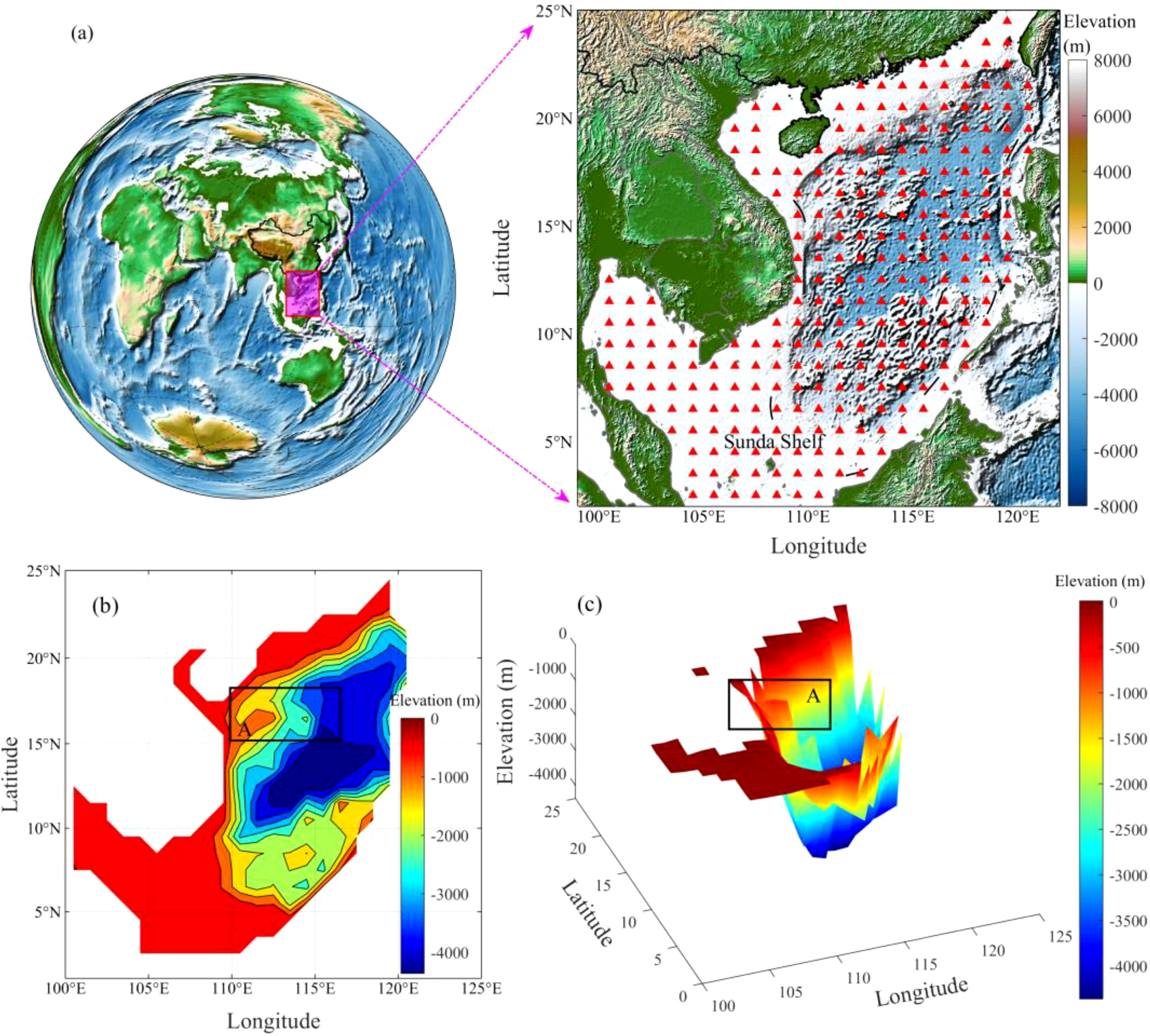
Figure 1. Geographical location of the SCS and gridded points of altimetry SLAs distributed over the SCS (A) and the topography of the SCS (B, C) in this study.

2.2 Data description

From the Archiving, Validation, and Interpretation of Satellite Oceanographic (AVISO) data center, we obtained monthly SLA data gridded at 0.25°for 1993–2022, which were compiled from various satellite altimetric observations (e.g., T/P, Jason-1/2, ERS-1/2, and Envisat). To comprehensively analyze each component of SLA, monthly and 1°-gridded data products of the steric sea level (SSL) at 0–300 m depths from 1993 to 2022 were also employed. The SSL data products were calculated by integrating temperature and salinity data by Cheng et al. (2017). The datasets are publicly accessible at http://www.ocean.iap.ac.cn. Another component of SLA is the non-steric sea level (NSSL), which is calculated by subtracting the inverted barometer correction from gravity recovery and climate experiment (GRACE)-derived ocean bottom pressure data (Willis et al., 2008). For the calculation of ocean bottom pressure, the GRACE Level-2 Release 06 (RL06) Stokes’ coefficients from the Center for Space Research (CSR), the GeoForschungsZentrum Potsdam (GFZ), and the Jet Propulsion Laboratory (JPL) from 2003 to 2015 were employed. After the low-degree coefficients were corrected via satellite laser ranging data [cf. Swenson et al. (2008)] for detailed procedures), the ocean bottom pressure was destriped and Gaussian spatially-smoothed at 500 km to minimize uncertainties (Swenson and Wahr, 2006). The three datasets were then averaged to minimize noise further and resampled into 1°×1° gridded solutions for calculating the NSSL.

The sea surface temperature (SST) dataset provided by the Met Office Hadley Centre, known as HadISST, which has a 1°×1° spatial resolution from 1993 to 2022, was also utilized. These datasets underwent reconstruction via a two-stage reduced-space optimal interpolation procedure, followed by the superposition of quality-improved gridded observations onto the reconstructions to restore local detail (see Rayner et al. (2003) for details). The data can be accessed at https://www.metoffice.gov.uk/hadobs/hadisst/.

In this study, the satellite-altimetric SLA was resampled to 1°×1° to unify the spatial resolution with other datasets, with grid points within the SCS shown in Figure 1.

3 Methods

To elaborate on the framework of our study, a flowchart depicting the experimental steps is summarized in Figure 2. The steps consisted of three main parts: (1) data analysis; (2) model establishment; and (3) accuracy evaluation. As part of the data analysis, the empirical orthogonal function (EOF) was employed to decompose the ENSO-related oceanic quantities (i.e., NSSL, SSL, SLA, and SST) in the equatorial Pacific (Section 3.1). Wavelet coherence (WCO) was utilized to highlight the relationship of the first EOF temporal model (PC1) time series between NSSL/SSL/SLA and SST (Section 3.2). Cross-correlation revealed the lagged relationship between NSSL/SSL/SLA/SST PC1 and the SCS interannual SLA (Section 3.3). On the basis of the above results, the PC1 time series of SSL/SLA/SST and interannual the SCS SLA at the adjacent 1–3 months were identified as focus and auxiliary regressors for training the model in this study. Additionally, the Lindeman, Merenda and Gold (LMG) method for relative importance analysis was used to calculate the weights of SSL/SLA/SST to the SCS interannual SLA for the weighted average time lag ($\text{Δ}t$). Finally, the Lag-WALS model parameters were estimated through the weighted-average least squares (WALS) procedure, thereby predicting the interannual SLA in the SCS. Details of the WALS and Lag-WALS model calculation steps are provided in Section 3.4 and Section 5.1, respectively. Due to limitations in the GRACE-derived NSSL data time span, the period for the data analysis part was uniformly set to 2003–2015. For model establishment, the data period was unified during 1993–2022 because the interannual variation of the GRACE-derived NSSL was negligible.

Figure 2

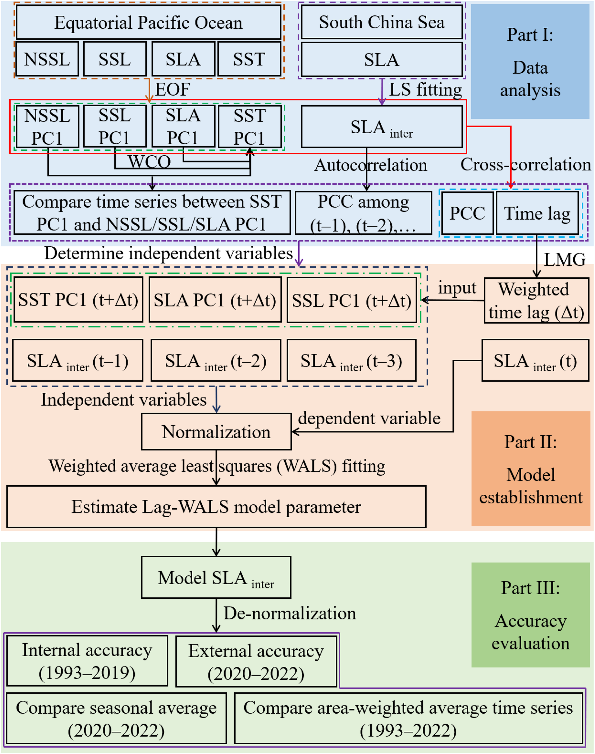
Figure 2. Flowchart for SLA forecast via the Lag-WALS approach.

3.1 Empirical orthogonal function

EOF, or principal component analysis (PCA), is a common method for extracting dominant spatiotemporal modes in gridded meteorological and climate datasets (Zou et al., 2021). To prevent the reordering of EOF modes caused by trends and seasonal variability, the trend and seasonal signals for each equatorial Pacific variable (SST, SLA, SSL, and NSSL) were removed beforehand via least squares (LS) fitting. As a result, the PC1 time series for SST, SLA, SSL, and NSSL in the equatorial Pacific were obtained, reflecting their ENSO representative characteristics (Ashok et al., 2007). The process of EOF decomposition involves two steps (Hannachi et al., 2007):

First, the spatiotemporal gridded data are represented in matrix form as follows:

$\begin{array}{ll}W=\left[\begin{array}{cc}\begin{array}{ccc}{w}_{11}& w_{12}& \dots \\ w_{21}& w_{22}& \dots \\ ⋮& ⋮& \ddots \end{array}& \begin{array}{c}{w}_{1n}\\ w_{2n}\\ ⋮\end{array}\\ \begin{array}{ccc}{w}_{m1}& w_{m1}& \dots \end{array}& w_{mn}\end{array}\right]& (1)\end{array}$

Where $w_{mn}$ represents the observed values of the SST, SLA, SSL, and NSSL at the corresponding position m and time n. Then, the anomaly field, $W_x$, can be defined as:

$\begin{array}{ll}{W}_x=W-{\left(P^T\left(\frac{1}{N}P{W}^T\right)\right)}^T& (2)\end{array}$

where P is the identity matrix composed of N ones in the diagonals.

The covariance matrix D is then calculated as:

$\begin{array}{ll}D=W_x\cdot W_{x }^T& (3)\end{array}$

Finally, the spatial modes and time coefficients are obtained from the eigenvalues and eigenvectors of covariance matrix D.

3.2 Wavelet coherence

WCO is the covariance strength of two time series in the time‒frequency domain calculated by wavelet coefficients. It provides a clear and intuitive representation of the linear or nonlinear correlation between two time series over time and frequency (Grinsted et al., 2004). In this study, we applied WCO to explore the relationship between SLA/SSL/NSSL PC1 (x) and SST PC1 (y). The wavelet coherence between two time series x and y is represented as:

$\begin{array}{ll}{R}_n^2(s)=\frac{{\left|S(s^{-1}{W}_n^{xy}(s))\right|}^2}{S\left(s^{-1}{\left|W_n^x(s)\right|}^2\right)\cdot S\left(s^{-1}{\left|W_n^y(s)\right|}^2\right)}& (4)\end{array}$

where s is the scale; S is the smoothing operator; $W_n^x(s)$ and $W_n^y(s)$ are the continuous wavelet transforms of time series x and y, respectively. $W_n^{xy}(s)$ is a cross-spectrum of the x and y time series. A more detailed description can be found in Grinsted et al. (2004).

3.3 Cross-correlation

To reveal the lagged effect and strength between the SCS SLA and equatorial Pacific oceanic variables (i.e., SST, SLA, SSL, and NSSL), the cross-correlation coefficient (Yang et al., 2024), $R(\tau )$, between the SCS SLA (X) and equatorial Pacific oceanic variables (Y) is formulated as:

$\begin{array}{ll}R(\tau )=\frac{{\delta }_{12}(\tau )}{\sqrt{{\delta }_{11}{\delta }_{22}}}& (5)\end{array}$

where ${\delta }_{12}$ is the cross-covariance of X and Y; ${\delta }_{11}$ and ${\delta }_{22}$ are the variances of X and Y; and $\tau$ is the time lag between X and Y, ranging from –12 to 12 months in our study.

3.4 Weighted-average least squares

WALS is a relatively novel model averaging method that is designed to address the model uncertainty resulting from model selection introduced in 2010 (Magnus and De Luca, 2016). Compared with the Akaike information criterion (AIC), the Bayesian information criterion (BIC), the combined criterion (ABIC) (Fok and Liu, 2019; Liu et al., 2019) or frequency theory alternatives, employing semiorthogonal transformations of regression equations (Magnus et al., 2010; Rahman et al., 2020) substantially reduces the computational burden. The estimation process of WALS includes the following steps (detailed in Magnus et al. (2010) and Magnus and De Luca (2016)):

1. Set up a linear regression model with the target data, y ($n\times 1$), expressed as:

$\begin{array}{ll}y=X_1{\beta }_1+X_2{\beta }_2+ϵ& (6)\end{array}$

where $X_1$ is the $n\times p$ focus regressor matrix, $X_2$ is the $n\times q$ auxiliary regressor, $ϵ\sim \text{N}(0, {\sigma }^2{I}_n)$ is the $n\times 1$ random error vector, ${\sigma }^2$ represents the error variance, $I_n$ is an $n\times n$ identity matrix, and ${\beta }_1$($p\times 1$) and ${\beta }_2$($q\times 1$) are unknown parameter vectors to be estimated in the following steps.

2. Calculate a projection matrix M as follows:

$\begin{array}{ll}M=I_n-X_1{({X^{\prime }}_1{X}_1)}^{-1}{X^{\prime }}_1& (7)\end{array}$

where M is a symmetric matrix. Thus, we can define $M{X}_2$ whose columns are orthogonal to the columns of $X_1$. The columns of $M{X}_2$ can be orthogonalized through $(M{X}_2{)}^{\prime }(M{X}_2)={X^{\prime }}_{2}M{X}_2$, followed by diagonalizing ${X^{\prime }}_{2}M{X}_2$ through

$\begin{array}{ll}{P}^{\prime }{X^{\prime }}_{2}M{X}_{2}P=\text{Λ}& (8)\end{array}$

where P is an orthogonal $q\times q$ matrix, and $\text{Λ}$ is a diagonal matrix whose diagonal elements are the corresponding eigenvalues. Through P and $\text{Λ}$, we can define a new orthogonalized auxiliary regressor $X_2^{*}$ and a new regression parameter vector ${\beta }_2^{*}$ as in Equation 9.

$\begin{array}{ll}\begin{array}{l}{X}_2^{*}=X_{2}P{\text{Λ}}^{-1/2}\\ {\beta }_2^{*}={\text{Λ}}^{1/2}{P}^{\prime }{\beta }_2\end{array}& (9)\end{array}$

where $X_2^{*}{\beta }_2^{*}=X_2{\beta }_2$ and $X_2^{*}\prime M{X}_2^{*}=I_q$. Thus, Equation 6 can also be expressed as $y=X_1{\beta }_1+X_2^{*}{\beta }_2^{*}+ϵ$, in which ${\beta }_1$ and ${\beta }_2^{*}$ are to be estimated.

3. Select the k-th model selection for the auxiliary variables such that $m_k$ is expressed as

$\begin{array}{ll}{m}_k=\left\{X_1{\beta }_1+X_2^{*}k{\beta }_2^{*}k+ϵ\right\}& (10)\end{array}$

where $X_{2k}^{*}=X_2^{*}{V}_k$ and $k=1,\cdots 2^q$. $V_k=diag(v_{k1},\cdots ,v_{kj})$ is an $q\times q$ diagonal matrix with diagonal elements $v_{kj}\in \left\{0,1\right\}, j=1,\cdots ,q$. Then, the least squares estimators of ${\beta }_1$ and ${\beta }_2^{*}$ under model $m_k$ are given by Equation 11.

$\begin{array}{ll}\begin{array}{l}{\widehat{\beta }}_{1k}={(X_1^{\prime }{X}_1)}^{-1}{X}_1^{\prime }y-Q^{*}{V}_k{\widehat{\beta }}_2^{*}\\ {\widehat{\beta }}_{2k}^{*}=V_k{X}_2^{*}\prime My\end{array}& (11)\end{array}$

where $Q^{*}={(X_1^{\prime }{X}_1)}^{-1}{X}_1^{\prime }{X}_2^{*}$. Because $ϵ\sim \text{N}(0, {\sigma }^2{I}_n)$, the joint distribution of ${\widehat{\beta }}_{1k}$ and ${\widehat{\beta }}_{2k}^{*}$ is expressed as follows:

$\begin{array}{ll}\left(\begin{array}{c}{\widehat{\beta }}_{1k}\\ {\widehat{\beta }}_{2k}^{*}\end{array}\right)\sim N\left(\left(\begin{array}{c}{\beta }_1+Q^{*}(I_q-V_k){\widehat{\beta }}_{2k}^{*}\\ V_k{\widehat{\beta }}_{2k}^{*}\end{array}\right),{\sigma }^2\left(\begin{array}{cc}{(X_1^{\prime }{X}_1)}^{-1}+Q^{*}{V}_k{Q}^{*\text{'}}& -Q^{*}{V}_k\\ -V_k{Q}^{*\text{'}}& V_k\end{array}\right)\right)& (12)\end{array}$

4. Define the WALS estimator of ${\beta }_{1k}$ as

$\begin{array}{ll}{b}_1={\displaystyle \sum _{k=1}^K{\lambda }_k{\widehat{\beta }}_{1k}}& (13)\end{array}$

where the weight function ${\lambda }_k\ge 0$ is assumed to be satisfied with the following conditions:

$\begin{array}{ll}{\displaystyle \sum _k{\lambda }_k=1{\lambda }_k}={\lambda }_k\left({\widehat{\beta }}_2^{*},s^2\right)& (14)\end{array}$

where $s^2$ is the estimator of ${\sigma }^2$ in the unrestricted model (all auxiliary variables are used). ${\widehat{\beta }}_2^{*}=X_{\mathrm{2 }\text{'}}^{*}My$. Under this assumption, the WALS estimator of ${\beta }_{1k}$ can then be written as

$\begin{array}{ll}\begin{array}{l}{b}_1={({X^{\prime }}_1{X}_1)}^{-1}{X^{\prime }}_{1}y-Q^{*}V{\widehat{\beta }}_2^{*}\\ V={\displaystyle \sum _k{\lambda }_k{V}_k}\end{array}& (15)\end{array}$

5. Let $\widehat{\eta }={\widehat{\beta }}_2^{*}/\sigma$, which implicitly implies that ${\widehat{\eta }}_j\sim N({\eta }_j,1), j=1,\cdots ,q$. The Laplace estimator ${\overline{\eta }}_j$ is subsequently calculated via Equation 16 to determine how ${\eta }_j$ must be estimated.

$\begin{array}{ll}{\overline{\eta }}_j=E({\eta }_j|{\widehat{\eta }}_j)=\frac{1+h({\widehat{\eta }}_j)}{2}({\widehat{\eta }}_j-c)+\frac{1-h({\widehat{\eta }}_j)}{2}({\widehat{\eta }}_j+c)& (16)\end{array}$

where $h({\widehat{\eta }}_j)=\frac{e^{-c{\widehat{\eta }}_j}\varphi ({\widehat{\eta }}_j-c)-e^{c{\widehat{\eta }}_j}\varphi (-{\widehat{\eta }}_j-c)}{e^{-c{\widehat{\eta }}_j}\varphi ({\widehat{\eta }}_j-c)+e^{c{\widehat{\eta }}_j}\varphi (-{\widehat{\eta }}_j-c)}$ and $\varphi$ denote the cumulative distribution functions of the standard normal distribution. $c=\log 2$ (Seya et al., 2014). Define $\overline{N}={({\overline{\eta }}_1,\cdots ,{\overline{\eta }}_q)}^{\prime }$.

6. According to the above processing, the WALS estimators of ${\beta }_2$ and ${\beta }_1$ are presented as follows:

$\begin{array}{ll}{\beta }_2=\sigma P{\text{Λ}}^{-1/2}\overline{N}{\beta }_1={({X^{\prime }}_1{X}_1)}^{-1}{X^{\prime }}_1(y-X_2{\beta }_2)& (17)\end{array}$

In this study, the focus and auxiliary variables are chosen to be the lagged equatorial Pacific ENSO-related quantities and the SCS interannual SLA in three adjacent months, forming a Lag-WALS model for the parameter estimation (c.f., Section 5.1).

4 Analysis of equatorial Pacific ENSO-related quantities and their associations with SCS SLA

4.1 Comparing time series between SST and SLA/SSL/NSSL in the equatorial Pacific

Following previous studies, we performed an EOF analysis of SST in the equatorial Pacific, revealing that the first EOF mode represents the conventional ENSO phenomenon (Ashok et al., 2007; Li et al., 2019). The same procedure is applied to the SLA, SSL, and NSSL (Figures 3A–E). The first spatial model (EOF1) of SLA and SSL exhibits strong similarities with SST, and a typical ENSO horseshoe spatial pattern in SST can be revealed in EOF1 of SLA and SSL (Figures 3A–C). Furthermore, the changes in the first EOF temporal mode (i.e., PC1) also confirm the consistent variability of SLA/SSL with SST, with a high correlation coefficient of 0.93 (Figure 3E). In contrast to SLA and SSL, NSSL PC1 displays large disparities, yielding a low correlation coefficient of 0.39 with SST in addition to the spatial pattern manifested from NSSL EOF1 (Figures 3D, E). This suggests weak or even no ENSO-related signals in NSSL.

Figure 3

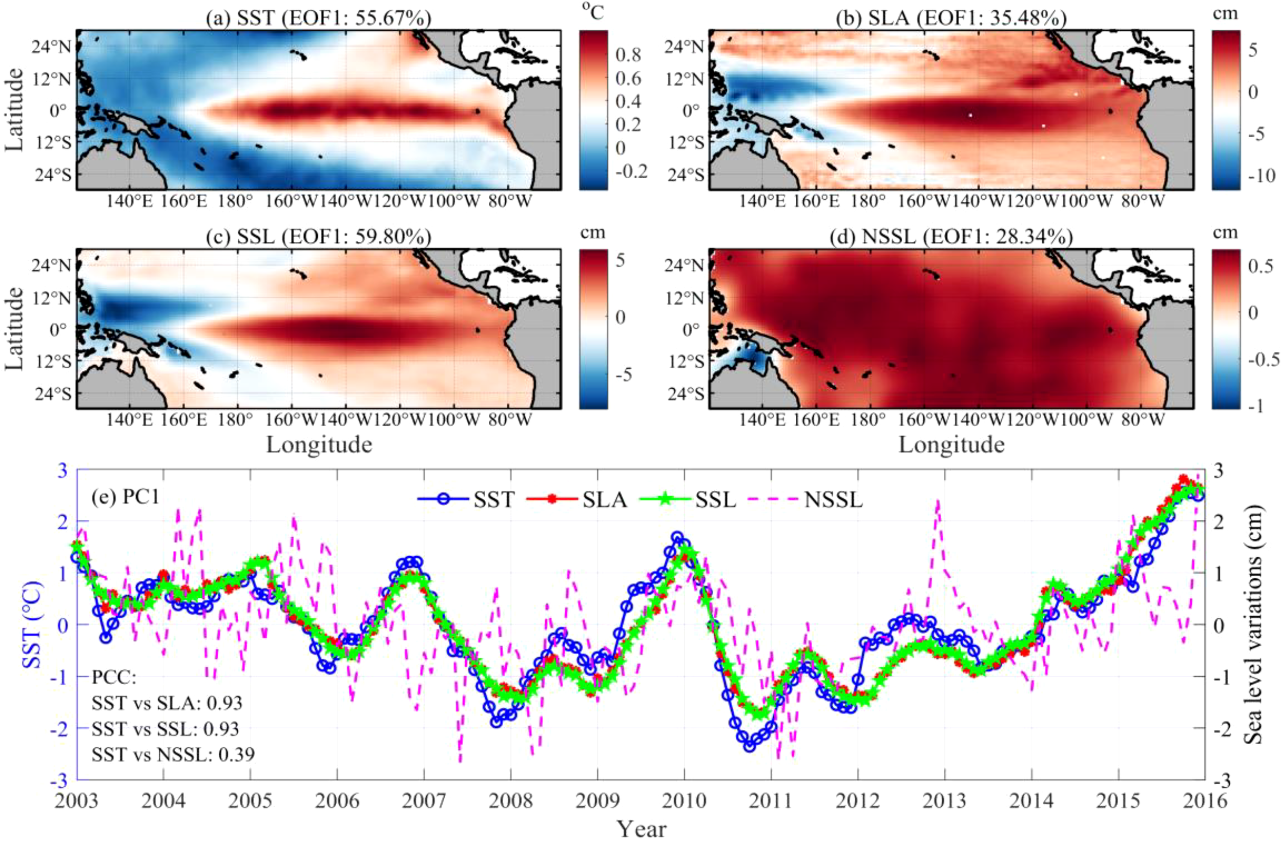
Figure 3. Spatiotemporal pattern of the first mode of SST, SLA, SSL, and NSSL in the equatorial Pacific based on the EOF method. (A–D) are the first modes of the spatial distributions of SST, SLA, SSL, and NSSL (i.e., EOF1), respectively. (E) Is the first mode of the time series of the time coefficients of SST, SLA, SSL, and NSSL (i.e., PC1).

To confirm the above speculation, WCO spectra between the PC1 time series of SST and SLA (SSL or NSSL) were computed (Figures 4A–C). Strong (weak) coherences between SST and SLA/SSL (NSSL) are exhibited in the WCO spectra with statistical significance higher than 95% at timescales between 1 and 4 years. This can be explained by the consistent phase (i.e., direction) between the SST and SLA/SSL vectors, which has common interannual variability (Figures 4A, B). The NSSL and SST, however, differ by approximately –90° in phase, implying that both are orthogonal to (i.e., independent of) each other (Figure 4C). This confirms that weak or even no ENSO-related signals are present in NSSL.

Figure 4

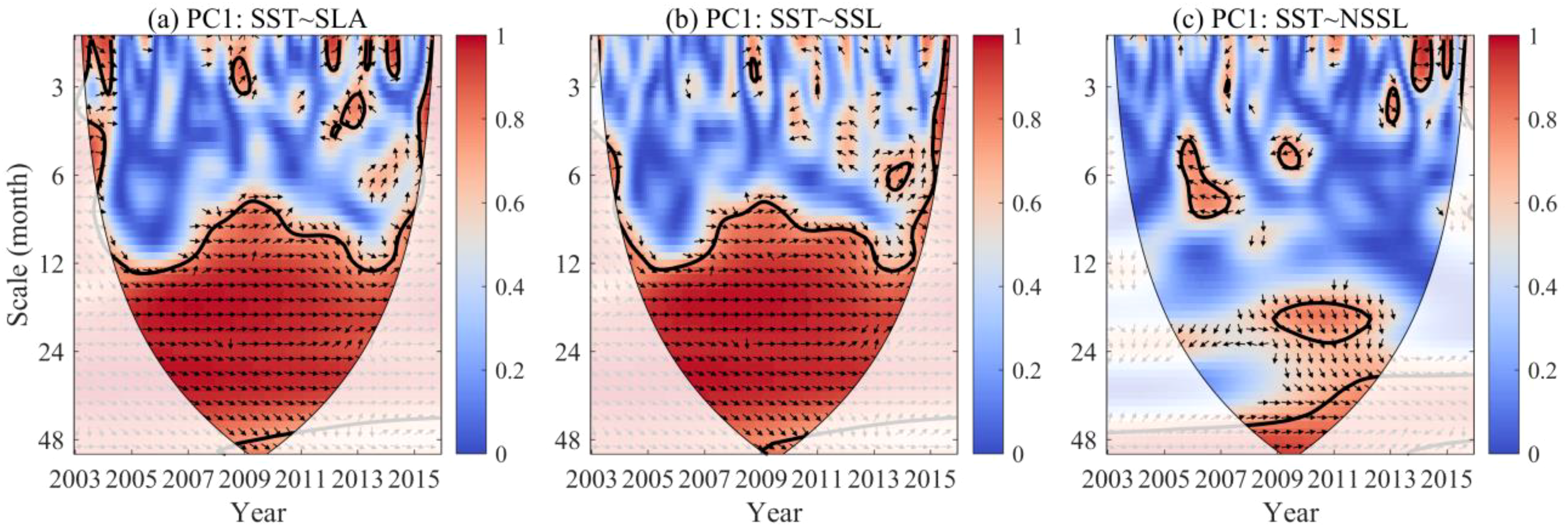
Figure 4. WCO analysis between SST PC1 and SLA PC1 (A), SSL PC1 (B), and NSSL PC1 (C). The arrow in an up direction (i.e., π/2) means that the SST leads the SLA/SSL/NSSL time series by 3 months.

4.2 Analysis of the cross-correlation between the SST/SLA/SSL/NSSL PC1 and SCS SLA

The mechanism of the influence of ENSO on the SCS SLA is believed to involve atmospheric circulation and the intrusion of the Kuroshio Current (Rong et al., 2007, 2009; Xi et al., 2019b; Xiong et al., 2023; Yang et al., 2024). Given the above coherence between the PC1 time series of the equatorial Pacific SLA/SSL/NSSL and SST, we further tested the consistency via cross-correlation analysis between the equatorial Pacific SLA/SSL/NSSL/SST and the interannual SLA in the SCS. We found that the spatial pattern of the maximum cross-correlation between the SCS SLA and SLA/SSL PC1 (NSSL PC1) was similar (different) to (from) that between SST PC1 (Figure 5). This finding indicates that the time series of the equatorial Pacific SLA and SSL PC1 can affect the interannual SCS SLA, as can the SST PC1. The resulting spatial distribution of the maximum cross-correlation between the SST/SLA/SSL PC1 and the SCS SLA indicates a significant impact of ENSO on the southeastern coastal boundaries of the SCS, which is consistent with the findings of Soumya et al. (2015). This characteristic may be attributed to the geographical setting in which the eastern boundary of the SCS is adjacent to the western Pacific, where ENSO-related coastal Kelvin waves can propagate to the southeastern SCS through the Mindoro Strait, inducing negative (positive) SLA variations during El Niño (La Niña) events (Liu et al., 2011). A relatively weak correlation was found between the SST/SLA/SSL PC1 and the SCS SLA in the interior SCS, which may be related to the wind-stress curl anomalies associated with ENSO and local wind patterns that can dampen the SLA variability in the central SCS (Cheng et al., 2016). During the mature phase of El Niño in winter, an anomalous anticyclone dominates the SCS (Wu et al., 2003), leading to downwelling in the central basin where the SLA is expected to increase. The opposite situation occurs during La Niña events (Wang et al., 2018). Additionally, the topography of the SCS, characterized by an abyssal plain with a mean depth of 4300m, may also influence the spatial distribution of this correlation (Wang et al., 2018).

Figure 5

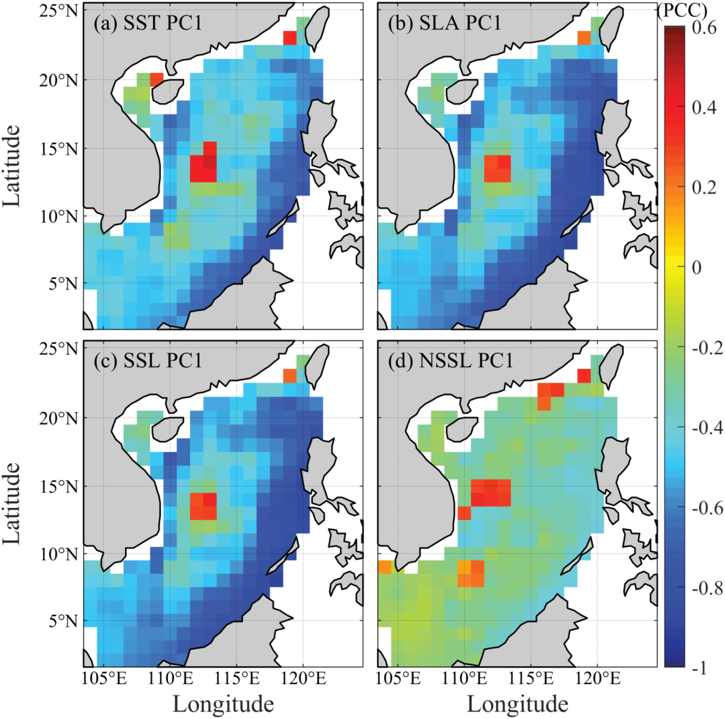
Figure 5. Spatial distributions of the maximum cross-correlations between SCS SLA interannual variations and SST PC1 (A), SLA PC1 (B), SSL PC1 (C), and NSSL PC1 (D).

Figure 6 also shows the spatial patterns of the time lag corresponding to the maximum cross-correlation. Again, we find that the time lag pattern between SLA/SSL PC1 (NSSL PC1) and the SCS SLA is consistent (inconsistent) with that of SST PC1. This further demonstrates that the PC1 time series of the SLA and SSL almost synchronized with the SST response before affecting the SCS SLA. This is consistent with the wavelet coherence analysis results illustrated in Figure 4. This suggests that the SLA and SSL could be indices equivalent to SST in revealing the time lag between ENSO-related signals and the interannual SCS SLA.

Figure 6

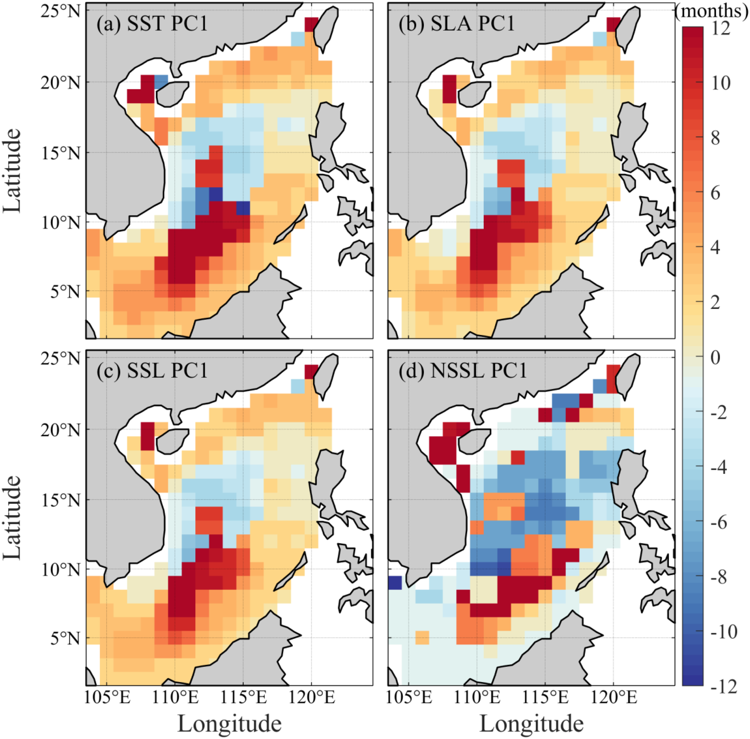
Figure 6. Spatial distributions of lags times between SCS SLA interannual variations and SST PC1 (A), SLA PC1 (B), SSL PC1 (C), and NSSL PC1 (D). The positive (negative) value represents the SCS SLA lag (lead).

In summary, a significant correlation between the SCS SLA and SST/SLA/SSL PC1 is found, with most grid points showing the maximum cross-correlation when the SCS SLA lags the SST, SLA, and SSL by several months. It is anticipated that interannual sea level variations in the SCS can be predicted in advance on the basis of ENSO-related SST/SLA/SSL variations. Therefore, the SST, SLA, and SSL PC1 time series were used to establish the SCS interannual SLA prediction model in Section 5.1.

4.3 Analysis of the temporal autocorrelation of the interannual SCS SLA

The interannual SCS SLA also affects itself by the previous months (Fu et al., 2019; Zhao et al., 2021). In other words, an autoregressive time lag pattern exists for the interannual SLA in the SCS. To illustrate this, the cosine (latitude) weighting scheme was employed to calculate the spatially averaged interannual SCS SLA time series followed by calculating its time autocorrelation. Figure 7 depicts the correlation matrix of the average interannual SCS SLA in the adjacent months. We found that the interannual SCS SLA yields high time autocorrelation coefficients for the adjacent three months (i.e., > 0.8), indicating a moderately strong relationship between the current interannual SLA and the previous three months. The shorter the time interval, the greater the autocorrelation. This implies the potential use of the interannual SLA from the previous month for forecasting the future interannual SLA. Therefore, the interannual SLA for the past three months was used as an auxiliary variable to constrain the forecasted interannual SCS SLA in the Lag-WALS model.

Figure 7

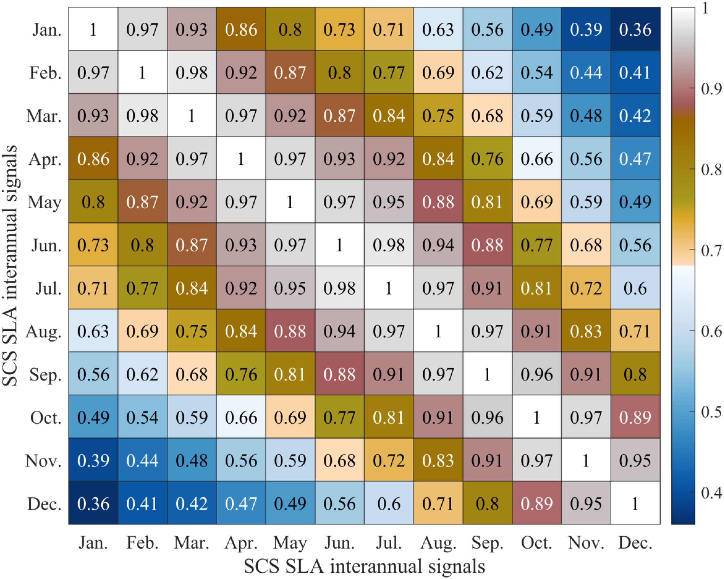
Figure 7. Correlation matrix with a heatmap of the SCS SLA interannual signals among adjacent months.

5 Establishing the Lag-WALS model and evaluating its accuracy

5.1 Lag-WALS model

In this study, we incorporated the autoregressive property of the SCS SLA and the time lag between each equatorial Pacific ENSO-related SST/SLA/SSL PC1 and SCS SLA into a Lag-WALS model based on the WALS method to forecast the interannual SCS SLA. The specific steps of establishing the Lag-WALS model are as follows:

1. Deseasonalize the SLA time series per grid to calculate the interannual SLA (SLA_inter) in the SCS via least-squares.

2. Determine the weighted-average time lag ($\text{Δ}t$) by first calculating the relative weight between each equatorial Pacific SST/SLA/SSL PC1 and the SCS SLA via the LMG relative importance algorithm (find Grömping (2007) for details), followed by simple weighted averaging.

3. Establish the Lag-WALS model through ENSO-related quantities in the equatorial Pacific (i.e., SST, SLA, SSL PC1; as focus regressors) and SCS SLA_inter at the adjacent 1–3 months (i.e., auxiliary regressors). Data from 1993–2019 (2020–2022) were selected as training (testing) data for model establishment and normalized before establishing the model to eliminate the influence of data magnitude and unit differences. The Lag-WALS model framework is as follows:

$\begin{array}{ll}\begin{array}{r}SL{A}_{\mathrm{int}er}(t)=(\begin{array}{ccc}SS{T}_{PC1}(t+\text{Δ}t)& SL{A}_{PC1}(t+\text{Δ}t)& SS{L}_{PC1}(t+\text{Δ}t))\end{array}\left(\begin{array}{c}{\beta }_{1,1}\\ {\beta }_{1,2}\\ {\beta }_{1,3}\end{array}\right)+\\ (\begin{array}{ccc}SL{A}_{\mathrm{int}er}(t-1)& SL{A}_{\mathrm{int}er}(t-2)& SL{A}_{\mathrm{int}er}(t-3)\end{array})\left(\begin{array}{c}{\beta }_{2,1}\\ {\beta }_{2,2}\\ {\beta }_{2,3}\end{array}\right)+ϵ\end{array}& (18)\end{array}$

where ${\beta }_{1,1}, {\beta }_{1,2}, {\beta }_{1,3}$ and ${\beta }_{2,1}, {\beta }_{2,2}, {\beta }_{2,3}$ are the coefficients of the Lag-WALS model; SST_PC1, SLA_PC1, and SSL_PC1 are the PC1 time series of the SST, SLA, and SSL in the equatorial Pacific; $SL{A}_{inter}$ is the interannual SLA in the SCS; t is the t-th epoch; $\text{Δ}t$ is the weighted average time lag; and $ϵ$ is a random vector of unobservable disturbances.

Then, the forecast $SL{A}_{inter}$ in the epoch, t, can be obtained via the Lag-WALS model coefficient, $\beta$, solved via Equation 18. Note that the $SL{A}_{inter}$ prediction values must be denormalized to restore their data magnitude.

5.2 Internal and external accuracy of the Lag-WALS model

To evaluate the performance of the Lag-WALS model, both internal and external accuracies are assessed in terms of the standard deviation (STD), root-mean-square error (RMSE), mean absolute error (MAE), and Bias (Fok et al., 2011; He et al., 2018; Ma et al., 2022). The STD, MAE, and Bias for the internal accuracy of the Lag-WALS model from 1993 to 2019 in the SCS are relatively small (Figure 8). The resulting performance of the SCS boundaries is more accurate (i.e., a lower STD and MAE) than that of the central region. Their spatial patterns are largely similar to the maximum cross-correlation spatial pattern, as displayed in Figure 5. Figure 9 shows the RMSE, MAE, and Bias for the model’s external accuracy from 2020 to 2022. Similar conclusions are drawn, except for the outliers at particular locations. This finding indicates that the impact of ENSO might be a potential reason for the higher accuracy in coastal areas, as the maximum cross-correlation between the interannual SLA and ENSO is greater in coastal areas than in the central SCS (Figure 5). This finding is consistent with the previous literature discussed in Section 4.2.

Figure 8

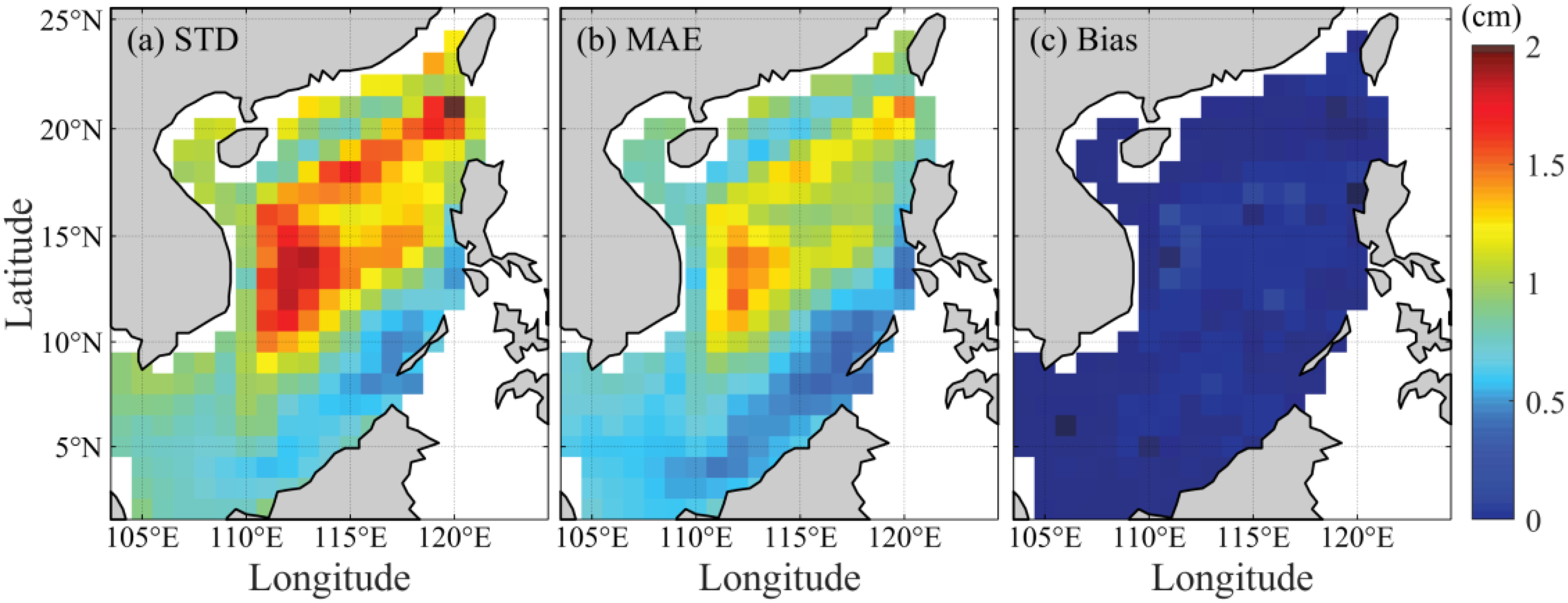
Figure 8. (A) STD, (B) MAE, and (C) Bias for the internal accuracy of the Lag-WALS model from 1993 to 2019.

Figure 9

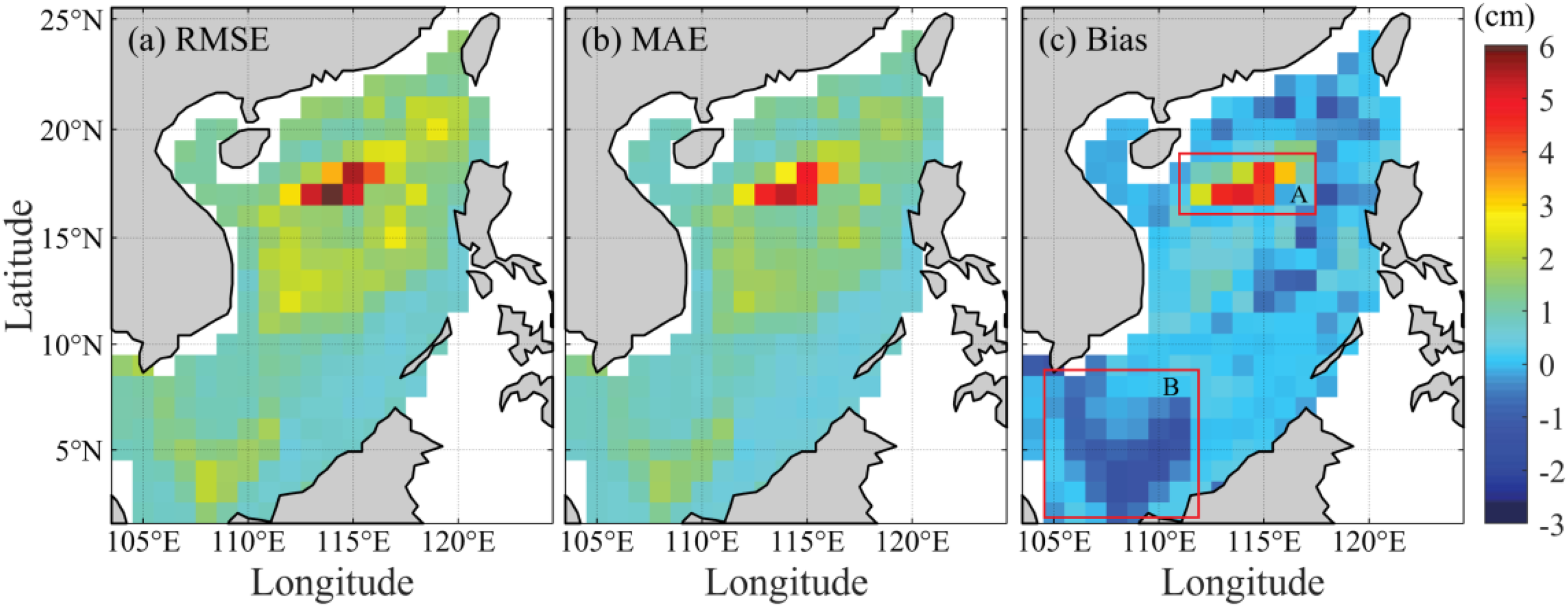
Figure 9. (A) RMSE, (B) MAE, and (C) Bias for the external accuracy of the Lag-WALS model from 2020 to 2022.

Another reason for the higher accuracy in coastal areas is that SSL significantly alters the SLA over deep water (Dangendorf et al., 2021), whereas NSSL substantially impacts the coastal SLA within the SCS (Cheng and Qi, 2010). Note that SSL and NSSL are two major SLA components. In this study, SSL data products, which were calculated on the basis of the integration of temperature and salinity data by Cheng et al. (2017), were downloaded at http://www.ocean.iap.ac.cn. The temperature and salinity data used to calculate the SSL are mostly reanalysis data. Different results are present among different SSL data products owing to different datasets and processing strategies (Camargo et al., 2020), thus resulting in unreliable SSL estimates over deep water. Coastal regions are shallower than SSL-dominated regions, such that fewer vertical depth structures are present. This makes the impact of NSSL dominate the coastal SLA.

Two notable regions with apparent error features are found. One is the abnormally high positive values in Box A of Figure 9, which is attributable to significant bottom topography changes within the region (c.f., Figure 1). This observation is consistent with that of Xu et al. (2012), who highlighted that significant changes in the mean dynamic topography have significant impacts on the SLA in the central SCS. Additionally, tidally induced energy dissipation amplified over the rough slope topography with complex seamounts and canyons in the northern SCS (Chang et al., 2006) significantly contributes to extreme sea level variability in the SCS (Menéndez and Woodworth, 2010; Zhang and Sheng, 2015). The spatial distribution of sea level maxima in the SCS is also influenced by tropical cyclones (Feng and Tsimplis, 2014; Zhang and Sheng, 2015).

Box B should be attributed to our interannual SLA prediction model, which merely considers ENSO-related oceanic signals. In essence, ENSO contributes 30% to the SLA, whereas the Indian Ocean Dipole (IOD) contributes 40% to the SLA in the southwestern SCS (Soumya et al., 2015; Li J. et al., 2023). Additionally, decadal processes, such as the Pacific Decadal Oscillation (PDO) and North Pacific Gyre Oscillation (NPGO), can indirectly modulate the interannual SLA in the SCS via subsurface temperature and salinity (Zhou et al., 2012; Deng et al., 2013; Wang et al., 2021; Li J. et al., 2023). In the southeastern SCS and the northern Gulf of Thailand, the PDO accounts for ~30% of the interannual SLA (Soumya et al., 2015). Specifically, the SCS, located between the western Pacific and the Indian Oceans, is significantly affected by interannual and decadal sea level fluctuations linked to ENSO and the PDO in the Pacific Ocean, as well as the IOD in the Indian Ocean (Mohan and Vethamony, 2018). The PDO is the predominant source of interdecadal climate variability in the Northwest Pacific, defined via monthly SST anomalies in the Pacific poleward of 20°N (Mantua et al., 1997). The decadal variability in the SLA is governed primarily by the PDO, particularly in the northwestern region of the SCS (Cheng et al., 2016; Mohan and Vethamony, 2018). In contrast, the IOD and ENSO are more influential in explaining the interannual sea level variability in the eastern Indian Ocean and SCS. While the IOD predominantly drives interannual SLA variations in the eastern Indian Ocean, the ENSO is the primary influence on the SCS (Mohan and Vethamony, 2018). Nonetheless, the interannual SLA variability in certain areas of the SCS is also affected by the IOD and PDO. Therefore, the interannual SLA prediction accuracy in the SCS should be substantially improved when the combined effects of ENSO, the IOD, and the PDO are incorporated into Equation 18, albeit with potential overfitting. This represents the major limitation of this study. Another possibility is that the correction of glacial isostatic adjustment to satellite altimetry has been ignored potentially affecting the long-term trend, although its impact is relatively small (Huang et al., 2013), at approximately –0.3 mm/yr over the SCS (Feng et al., 2012).

Overall, the prediction accuracy (RMSE) of the Lag-WALS model in the SCS ranges from 0.49 to 5.93 cm, with average STD/MAE/Bias (RMSE/MAE/Bias) values of the model’s internal (external) accuracy in the SCS of 1.01/0.80/–0.002 cm (1.39/1.13/–0.08 cm), respectively (Table 1). Table 2 displays the prediction accuracy of all existing SLA prediction methods. The results obtained by the Lag-WALS method are comparable to those of the other methods. In particular, our resulting accuracy closely agrees with the best result of the hybrid prediction model proposed by Fu et al. (2019) over the SCS (i.e., RMSE: 1.32 cm; MAE: 1.03 cm). This finding indicates that our proposed model yields good reliability for interannual SLA estimates, whereas the calculation steps are simpler and computationally more efficient than those of Fu et al. (2019). Note that Fu et al. (2019) is a millimeter more accurate than our prediction, which is attributed to the greater number of involved steps and time-consuming data processing procedures.

Table 1

Table 1. Statistical results of the internal and external accuracies of the Lag-WALS model.

Table 2

Table 2. Accuracy (RMSE) statistics of existing SLA prediction methods.

To assess the performance of our proposed model seasonally, the forecasted interannual SLAs were compared with the altimetric observations from 2020 to 2022 across four seasons: spring (March to May), summer (June to August), autumn (September to November), and winter (December to February). The spatial patterns of the altimetric-observed mean interannual SCS SLA and the model-forecasted SLA for different seasons are shown in Figures 10A, B. Both patterns basically agree for each individual season. Notably, the model’s estimates in the central region of the SCS during summer exhibit a more diverse spatial pattern than those in the other three seasons. The residuals, which are the difference between the observed and model values (Figure 10C), are relatively small regardless of season. The regions with significant outliers are largely consistent with the findings shown in Figure 9, as the potential reasons discussed above. Overall, the statistics of the residuals for the four seasons are –0.14, 0.17, –0.06, and –0.28 cm, respectively (Table 3).

Figure 10

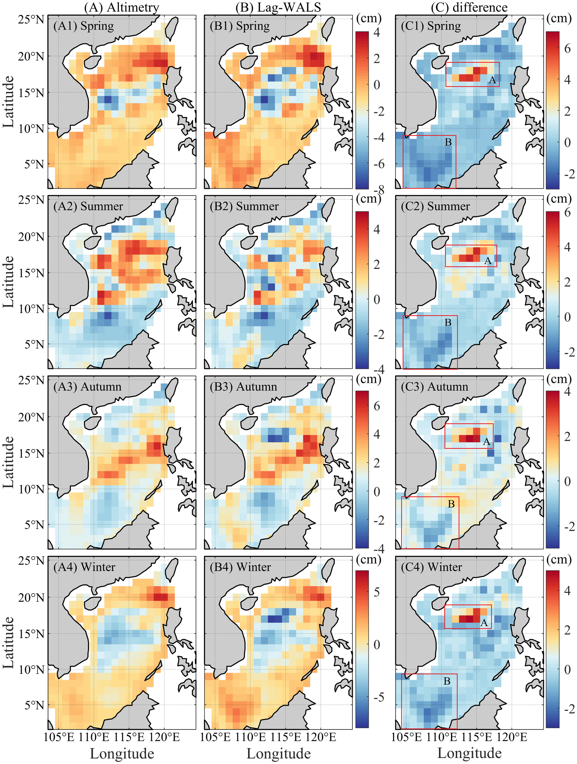
Figure 10. Mean interannual SCS SLA images derived from the altimetry (A) and Lag-WALS (B) models in different seasons and their differences (C) from 2020 to 2022. The numbers 1-4 represent spring, summer, autumn, and winter, respectively.

Table 3

Table 3. Mean values of the interannual SCS SLAs derived from altimetric observations and the Lag-WALS model and their differences across the four seasons.

In addition to the comparison with the observed values in different seasons, changes in regionally averaged time series were also analyzed. Figure 11 shows the changes in the regionally averaged time series of the observed and model values, along with their differences from 1993 to 2022. The comparison reveals a strong consistency between the observed and modeled time series changes, with differences mostly within ±1 cm. The RMSE and MAE of the training (testing) set for the difference between the observed and model values are 0.36 cm and 0.28 cm (0.49 cm and 0.39 cm), indicating that the relevant parameters obtained from the training set have good performance in the testing set (i.e., 2020–2022) and that the model did not exhibit overfitting issues in this study. Furthermore, we set the significance level at 0.05 during model training stage. This study focuses only on the interannual variation in the SLA, eliminating the influence of other signals, followed by normalizing the data during the model construction stage to avoid the impact of differences in data magnitude. These strategies effectively prevented the occurrence of overfitting issues in this study. The Lag-WALS model generally yields good reliability and higher accuracy in predicting the SCS SLA at the interannual scale.

Figure 11

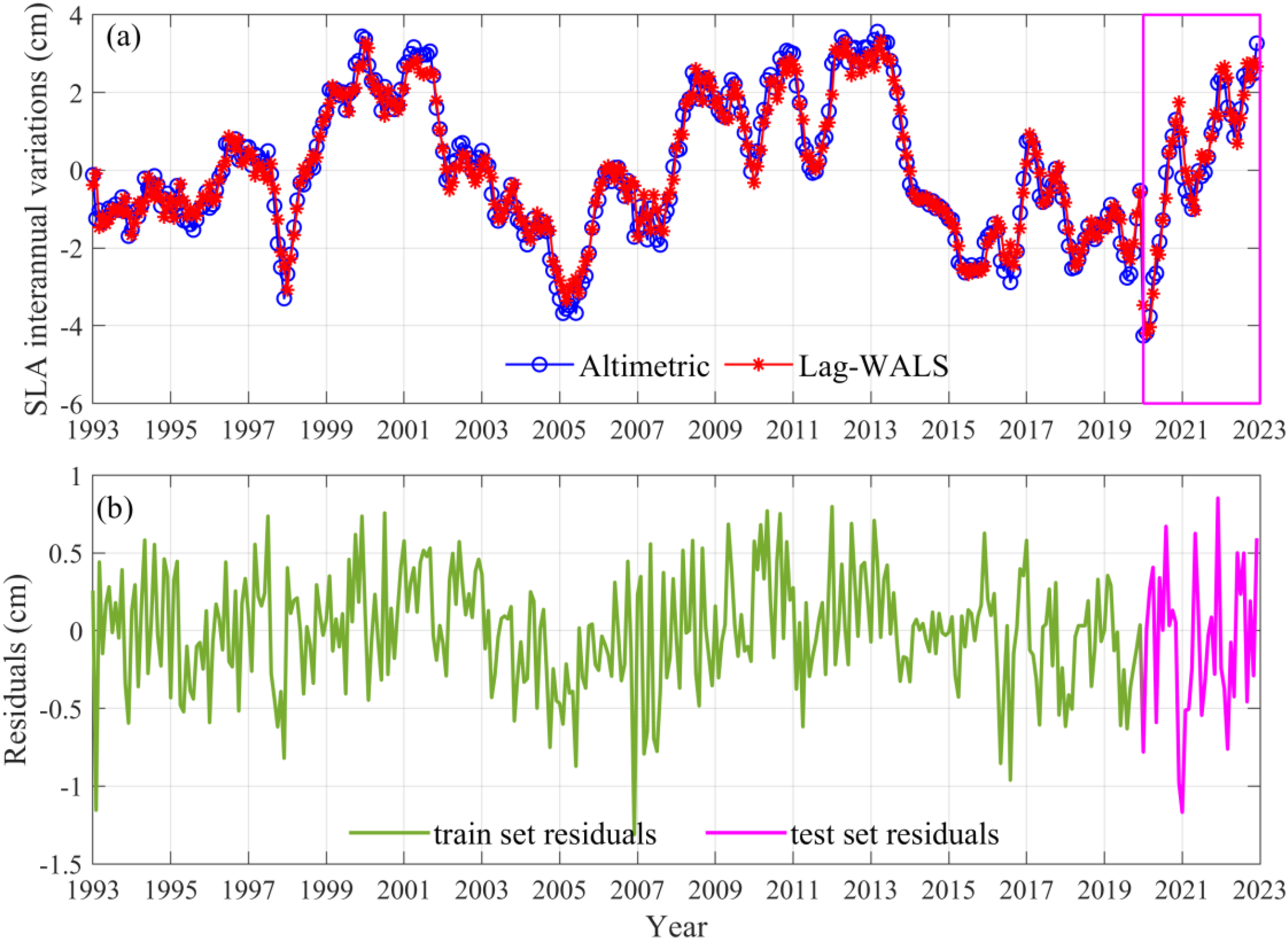
Figure 11. Regionally averaged time series of altimetric-observed and Lag-WALS model-predicted SLAs (A) and their differences (B) from 1993 to 2022. The pink matrix box represents the test set data (i.e., 2020–2022).

6 Conclusions

A novel Lag-WALS approach for forecasting interannual SLA variations in the SCS on the basis of lagged equatorial Pacific ENSO-related quantities was proposed in this study. We examined the relationships between the SST and SLA, along with its two primary components (SSL and NSSL) in the equatorial Pacific, and then investigated their cross-correlations with the interannual SCS SLA to identify regressors for the Lag-WALS model. Additionally, the interannual SCS SLAs for the adjacent three months served as auxiliary regressors to constrain the Lag-WALS model-predicted results.

Our analysis revealed a robust alignment between the first spatiotemporal mode of EOF (EOF1 and PC1) from SLA/SSL and SST across the equatorial Pacific, revealing a typical ENSO horseshoe spatial pattern in EOF1. In contrast, the NSSL showed significant disparities, indicating weak or even no ENSO-related signals. This finding was also confirmed via wavelet coherence analysis. The similar (different) spatial pattern of the maximum cross-correlation between the SCS SLA and SLA/SSL PC1 (NSSL PC1) to (from) that between SST PC1 further supported this inference. Furthermore, a high-time autocorrelation coefficient demonstrated that the interannual SCS SLA was also influenced by its previous months, suggesting the potential use of the interannual SLA in the previous months for forecasting the interannual SLA.

After the Lag-WALS model was established, its construction and prediction performances were internally and externally assessed. The model demonstrated greater accuracy at the SCS boundaries than in the central region, with average STD/MAE/Bias (RMSE/MAE/Bias) values of the model’s internal (external) accuracy in the SCS of 1.01/0.80/–0.002 cm (1.39/1.13/–0.08 cm). Both the altimetric and Lag-WALS model patterns basically for each individual season. The consistency of the regionally averaged time series changes between the observed and model values was also noted, with differences mostly within ±1 cm. The RMSE and MAE of the training (testing) set for the difference in the regional mean time series between the observed and model values were 0.36 cm and 0.28 cm (0.49 cm and 0.39 cm), respectively. These results underscore the ability of the Lag-WALS model to accurately forecast the SCS SLA at the interannual scale, which is vital for early detection of abnormal sea level changes.

The limitation of this study is that the model takes into account only the ENSO-related quantities and the previous month’s interannual SLA while ignoring potential influencing factors of the interannual SCS SLA, such as the IOD and PDO. Thus, incorporating multiple influencing factors should further improve the model’s performance. Furthermore, the solution method used in the Lag-WALS model is the least squares method, and employing a total least squares solution may further improve the model’s theoretical accuracy.

Data availability statement

Publicly available datasets were analyzed in this study. This data can be found here: https://www.aviso.altimetry.fr/; https://www.metoffice.gov.uk/hadobs/hadisst/; http://www.ocean.iap.ac.cn; http://icgem.gfz-potsdam.de.

Author contributions

PY: Conceptualization, Data curation, Formal analysis, Investigation, Methodology, Software, Validation, Visualization, Writing – original draft, Writing – review & editing. HF: Conceptualization, Data curation, Formal analysis, Funding acquisition, Investigation, Methodology, Project administration, Resources, Supervision, Writing – review & editing.

Funding

The author(s) declare financial support was received for the research, authorship, and/or publication of this article. This study is financed by the National Natural Science Foundation of China (Grant Nos. 41974003 & 41674007) and the Natural Science Foundation of Hubei Province, China (Grant No. 2022CFB064).

Acknowledgments

Thanks also to AVISO, GRACE, Met Office Hadley Centre, and the Ocean and Climate team of Institute of Atmospheric Physics for supplying the datasets, respectively. The monthly AVISO SLA datasets from https://www.aviso.altimetry.fr/, and SSL can be accessed at http://www.ocean.iap.ac.cn. The GARCE data calculated by Level-2 Release 06 (RL06) Stokes’ coefficients available at http://icgem.gfz-potsdam.de. The SST provided by Met Office Hadley Centre at https://www.metoffice.gov.uk/hadobs/hadisst/.

Conflict of interest

The authors declare that the research was conducted in the absence of any commercial or financial relationships that could be construed as a potential conflict of interest.

Publisher’s note

All claims expressed in this article are solely those of the authors and do not necessarily represent those of their affiliated organizations, or those of the publisher, the editors and the reviewers. Any product that may be evaluated in this article, or claim that may be made by its manufacturer, is not guaranteed or endorsed by the publisher.

References

Altunkaynak A., Kartal E. (2021). Transfer sea level learning in the Bosphorus Strait by wavelet based machine learning methods. Ocean Eng. 233, 109116. doi: 10.1016/j.oceaneng.2021.109116

Crossref Full Text | Google Scholar

Ashok K., Behera S. K., Rao S. A., Weng H., Yamagata T. (2007). El Niño Modoki and its possible teleconnection. J. Geophys. Res.-Oceans. 112, C11007. doi: 10.1029/2006JC003798

Crossref Full Text | Google Scholar

Camargo C. M. L., Riva R. E. M., Hermans T. H. J., Slangen A. B. A. (2020). Exploring sources of uncertainty in steric sea-level change estimates. J. Geophys. Res.-Oceans 125, e2020JC016551. doi: 10.1029/2020JC016551

Crossref Full Text | Google Scholar

Cazenave A., Palanisamy H., Ablain M. (2018). Contemporary sea level changes from satellite altimetry: What have we learned? What are the new challenges? Adv. Space Res. 62, 1639–1653. doi: 10.1016/j.asr.2018.07.017

Crossref Full Text | Google Scholar

Chang M. H., Lien R. C., Tang T. Y., D'Asaro E. A., Yang Y. J. (2006). Energy flux of nonlinear internal waves in northern South China Sea. Geophys. Res. Lett. 33, L03607. doi: 10.1029/2005GL025196

Crossref Full Text | Google Scholar

Chen P., Jamet C., Zhang Z., He Y., Mao Z., Pan D., et al. (2021). Vertical distribution of subsurface phytoplankton layer in South China Sea using airborne lidar. Remote Sens. Environ. 263, 112567. doi: 10.1016/j.rse.2021.112567

Crossref Full Text | Google Scholar

Chen X., Zhang X., Church J. A., Watson C. S., King M. A., Monselesan D., et al. (2017). The increasing rate of global mean sea-level rise during 1993–2014. Nat. Clim. Change 7, 492–495. doi: 10.1038/nclimate3325

Crossref Full Text | Google Scholar

Cheng L., Trenberth K. E., Fasullo J., Boyer T., Abraham J., Zhu J. (2017). Improved estimates of ocean heat content from 1960 to 2015. Sci. Adv. 3, e1601545. doi: 10.1126/sciadv.1601545

PubMed Abstract | Crossref Full Text | Google Scholar

Cheng X., Qi Y. (2010). On steric and mass-induced contributions to the annual sea-level variations in the South China Sea. Glob. Planet. Change 72, 227–233. doi: 10.1016/j.gloplacha.2010.05.002

Crossref Full Text | Google Scholar

Cheng X., Xie S. P., Du Y., Wang J., Chen X., Wang J. (2016). Interannual-to-decadal variability and trends of sea level in the South China Sea. Clim. Dyn. 46, 3113–3126. doi: 10.1007/s00382-015-2756-1

Crossref Full Text | Google Scholar

Cheng Y., Plag H. P., Hamlington B. D., Xu Q., He Y. (2015). Regional sea level variability in the bohai sea, yellow sea, and east China sea. Cont. Shelf Res. 111, 95–107. doi: 10.1016/j.csr.2015.11.005

Crossref Full Text | Google Scholar

Dangendorf S., Frederikse T., Chafik L., klinck J. M., Ezer T., Hamlington B. D. (2021). Data-driven reconstruction reveals large-scale ocean circulation control on coastal sea level. Nat. Clim. Change 11, 514–520. doi: 10.1038/s41558-021-01046-1

Crossref Full Text | Google Scholar

Deng W., Wei G., Xie L., Ke T., Wang Z., Zeng T., et al. (2013). Variations in the Pacific Decadal Oscillation since 1853 in a coral record from the northern South China Sea. J. Geophys. Res.-Oceans. 118, 2358–2366. doi: 10.1002/jgrc.20180

Crossref Full Text | Google Scholar

Fang J., Liu W., Yang S., Brown S., Nicholls R. J., Hinkel J., et al. (2017). Spatial-temporal changes of coastal and marine disasters risks and impacts in Mainland China. Ocean Coast. Manage. 139, 125–140. doi: 10.1016/j.ocecoaman.2017.02.003

Crossref Full Text | Google Scholar

Feng W., Zhong M., Xu H. Z. (2012). Sea level variations in the South China Sea inferred from satellite gravity, altimetry, and oceanographic data. Sci. China-Earth Sci. 55, 1696–1701. doi: 10.1007/s11430-012-4394-3

Crossref Full Text | Google Scholar

Feng X., Tsimplis M. N. (2014). Sea level extremes at the coasts of China. J. Geophys. Res.-Oceans. 119, 1593–1608. doi: 10.1002/2013JC009607

Crossref Full Text | Google Scholar

Fok H. S., Liu Y. (2019). An improved GPS-inferred seasonal terrestrial water storage using terrain-corrected vertical crustal displacements constrained by GRACE. Remote Sens. 11, 1433. doi: 10.3390/rs11121433

Crossref Full Text | Google Scholar

Fok H. S., Shum C. K., Yi Y., Araki H., Ping J., Williams J. G., et al. (2011). Accuracy assessment of lunar topography models. Earth Planets Space. 63, 15–23. doi: 10.5047/eps.2010.08.005

Crossref Full Text | Google Scholar

Fu Y., Zhou X., Sun W., Tang Q. (2019). Hybrid model combining empirical mode decomposition, singular spectrum analysis, and least squares for satellite-derived sea-level anomaly prediction. Int. J. Remote Sens. 40, 7817–7829. doi: 10.1080/01431161.2019.1606959

Crossref Full Text | Google Scholar

Griggs G., Reguero B. G. (2021). Coastal adaptation to climate change and sea-level rise. Water. 13, 2151. doi: 10.3390/w13162151

Crossref Full Text | Google Scholar

Grinsted A., Moore J. C., Jevrejeva S. (2004). Application of the cross wavelet transform and wavelet coherence to geophysical time series. Nonlinear Process Geophys 11, 561–566. doi: 10.5194/npg-11-561-2004

Crossref Full Text | Google Scholar

Grömping U. (2007). Relative importance for linear regression in R: the package relaimpo. J. Stat. Software 17, 1–27. doi: 10.18637/jss.v017.i01

Crossref Full Text | Google Scholar

Hallegatte S., Green C., Nicholls R. J., Corfee-Morlot J. (2013). Future flood losses in major coastal cities. Nat. Clim. Change 3, 802–806. doi: 10.1038/nclimate1979

Crossref Full Text | Google Scholar

Hamlington B. D., Gardner A. S., Ivins E., Lenaerts J. T., Reager J. T., Trossman D. S., et al. (2020). Understanding of contemporary regional sea-level change and the implications for the future. Rev. Geophys. 58, e2019RG000672. doi: 10.1029/2019RG000672

PubMed Abstract | Crossref Full Text | Google Scholar

Han G., Chen N., Kuo C. Y., Shum C. K., Ma Z. (2016). Interannual and decadal sea surface height variability over the northwest Atlantic slope. IEEE J. Sel. Top. Appl. Earth Observ. Remote Sens. 9, 5071–5078. doi: 10.1109/JSTARS.2016.2584778

Crossref Full Text | Google Scholar

Han G., Huang W. (2009). Low-frequency sea-level variability in the South China Sea and its relationship to ENSO. Theor. Appl. Climatol. 97, 41–52. doi: 10.1007/s00704-008-0070-0

Crossref Full Text | Google Scholar

Hannachi A., Jolliffe I. T., Stephenson D. B. (2007). Empirical orthogonal functions and related techniques in atmospheric science: A review. Int. J. Climatol. 27, 1119–1152. doi: 10.1002/joc.1499

Crossref Full Text | Google Scholar

He Q., Fok H. S., Chen Q., Chun K. P. (2018). Water level reconstruction and prediction based on space-borne sensors: A case study in the Mekong and Yangtze river basins. Sensors. 18, 3076. doi: 10.3390/s18093076

PubMed Abstract | Crossref Full Text | Google Scholar

Huang Z., Guo J. Y., Shum C. K., Wan J., Duan J., Fok H. S., et al. (2013). On the accuracy of glacial isostatic adjustment models for geodetic observations to estimate arctic ocean sea-level change. Terr. Atmos. Ocean. Sci. 24, 471–490. doi: 10.3319/TAO.2012.08.28.01(TibXS)

Crossref Full Text | Google Scholar

Imani M., You R. J., Chung-Yen K. (2013). Accurate Forecasting of the satellite-derived seasonal Caspian sea level anomaly using polynomial interpolation and holt-winters exponential smoothing. Terr. Atmos. Ocean. Sci. 24, 521. doi: 10.3319/TAO.2012.10.12.01(TibXS)

Crossref Full Text | Google Scholar

Imani M., You R. J., Kuo C. Y. (2014a). Caspian Sea level prediction using satellite altimetry by artificial neural networks. Int. J. Environ. Sci. Technol. 11, 1035–1042. doi: 10.1007/s13762-013-0287-z

Crossref Full Text | Google Scholar

Imani M., You R. J., Kuo C. Y. (2014b). Forecasting Caspian Sea level changes using satellite altimetry data (June 1992–December 2013) based on evolutionary support vector regression algorithms and gene expression programming. Glob. Planet. Change. 121, 53–63. doi: 10.1016/j.gloplacha.2014.07.002

Crossref Full Text | Google Scholar

Imani M., You R. J., Kuo C. Y. (2014c). Analysis and prediction of Caspian Sea level pattern anomalies observed by satellite altimetry using autoregressive integrated moving average models. Arab. J. Geosci. 7, 3339–3348. doi: 10.1007/s12517-013-1048-5

Crossref Full Text | Google Scholar

Jenner C. J., Thuy T. T. (2016). The South China Sea. Cambridge, UK: Cambridge University Press.

Google Scholar

Kurniawan A., Ooi S. K., Babovic V. (2014). Improved sea level anomaly prediction through combination of data relationship analysis and genetic programming in Singapore Regional Waters. Comput. Geosci. 72, 94–104. doi: 10.1016/j.cageo.2014.07.007

Crossref Full Text | Google Scholar

Li C., Cai R., Yan X. (2023). Assessment of the future changes in the socio-economic vulnerability of China’s coastal areas. Sustainability. 15, 5794. doi: 10.3390/su15075794

Crossref Full Text | Google Scholar

Li J., Tan W., Sun W., Yang L., Lin L., Fu Q. (2023). Seasonal–interannual–decadal variations of sea level in the South China Sea and connections with the tropical–subtropical Pacific. Int. J. Climatol. 43, 5196–5207. doi: 10.1002/joc.8140

Crossref Full Text | Google Scholar

Li L., Switzer A. D., Wang Y., Chan C. H., Qiu Q., Weiss R. (2018). A modest 0.5-m rise in sea level will double the tsunami hazard in Macau. Sci. Adv. 4, eaat1180. doi: 10.1126/sciadv.aat1180

PubMed Abstract | Crossref Full Text | Google Scholar

Li Y., Chen Q., Liu X., Xing N., Cheng Z., Cai H., et al. (2019). The first two leading modes of the tropical Pacific and their linkage without global warming. Earth Planet. Phys. 3, 157–165. doi: 10.26464/epp2019019

Crossref Full Text | Google Scholar

Liu Q., Feng M., Wang D. (2011). ENSO-induced interannual variability in the southeastern South China Sea. J. Oceanogr. 67, 127–133. doi: 10.1007/s10872-011-0002-y

Crossref Full Text | Google Scholar

Liu Y., Fok H. S., Tenzer R., Chen Q., Chen X. (2019). Akaike’s bayesian information criterion for the joint inversion of terrestrial water storage using GPS vertical displacements, GRACE and GLDAS in southwest China. Entropy. 21, 664. doi: 10.3390/e21070664

PubMed Abstract | Crossref Full Text | Google Scholar

Ma Y., Wu Y., Shao Z., Cao T., Liang B. (2022). Impacts of sea level rise and typhoon intensity on storm surges and waves around the coastal area of Qingdao. Ocean Eng. 249, 110953. doi: 10.1016/j.oceaneng.2022.110953

Crossref Full Text | Google Scholar

Magnus J. R., De Luca G. (2016). Weighted-average least squares (WALS): a survey. J. Econ. Surv. 30, 117–148. doi: 10.1111/joes.12094

Crossref Full Text | Google Scholar

Magnus J. R., Powell O., Prüfer P. (2010). A comparison of two model averaging techniques with an application to growth empirics. J. Econom. 154, 139–153. doi: 10.1016/j.jeconom.2009.07.004

Crossref Full Text | Google Scholar

Makarynskyy O., Makarynska D., Kuhn M., Featherstone W. E. (2004). Predicting sea level variations with artificial neural networks at Hillarys Boat Harbour, Western Australia. Estuar. Coast. Shelf Sci. 61, 351–360. doi: 10.1016/j.ecss.2004.06.004

Crossref Full Text | Google Scholar

Mantua N. J., Hare S. R., Zhang Y., Wallace J. M., Francis R. C. (1997). A Pacific interdecadal climate oscillation with impacts on salmon production. Bull. Amer. Meteorol. Soc 78, 1069–1080. doi: 10.1175/1520-0477(1997)078<1069:APICOW>2.0.CO;2

Crossref Full Text | Google Scholar

Menéndez M., Woodworth P. L. (2010). Changes in extreme high water levels based on a quasi-global tide-gauge data set. J. Geophys. Res.-Oceans 115, C10011. doi: 10.1029/2009JC005997

Crossref Full Text | Google Scholar

Mohan S., Vethamony P. (2018). Interannual and long-term sea level variability in the eastern Indian Ocean and South China Sea. Clim. Dyn. 50, 3195–3217. doi: 10.1007/s00382-017-3800-0

Crossref Full Text | Google Scholar

Niedzielski T., Kosek W. (2009). Forecasting sea level anomalies from TOPEX/Poseidon and Jason-1 satellite altimetry. J. Geodesy. 83, 469–476. doi: 10.1007/s00190-008-0254-5

Crossref Full Text | Google Scholar

Peng D., Palanisamy H., Cazenave A., Meyssignac B. (2013). Interannual sea level variations in the South China Sea over 1950–2009. Mar. Geod. 36, 164–182. doi: 10.1080/01490419.2013.771595

Crossref Full Text | Google Scholar

Rahman K. U., Shang S., Shahid M., Wen Y., Khan A. J. (2020). Development of a novel weighted average least squares-based ensemble multi-satellite precipitation dataset and its comprehensive evaluation over Pakistan. Atmos. Res. 246, 105133. doi: 10.1016/j.atmosres.2020.105133

Crossref Full Text | Google Scholar

Rayner N. A. A., Parker D. E., Horton E. B., Folland C. K., Alexander L. V., Rowell D. P., et al. (2003). Global analyses of sea surface temperature, sea ice, and night marine air temperature since the late nineteenth century. J. Geophys. Res.-Atmos. 108, 4407. doi: 10.1029/2002JD002670

Crossref Full Text | Google Scholar

Rong Z., Liu Y., Zong H., Cheng Y. (2007). Interannual sea level variability in the South China Sea and its response to ENSO. Glob. Planet. Change. 55, 257–272. doi: 10.1016/j.gloplacha.2006.08.001

Crossref Full Text | Google Scholar

Rong Z., Liu Y., Zong H., Xiu P. (2009). Long term sea level change and water mass balance in the South China Sea. J. OCEAN Univ. 8, 327–334. doi: 10.1007/s11802-009-0327-y

Crossref Full Text | Google Scholar

Seya H., Tsutsumi M., Yamagata Y. (2014). Weighted-average least squares applied to spatial econometric models: A monte carlo investigation. Geogr. Anal. 46, 126–147. doi: 10.1111/gean.12032

Crossref Full Text | Google Scholar

Shao Q., Li W., Hou G., Han G., Wu X. (2020). Mid-term simultaneous spatiotemporal prediction of sea surface height anomaly and sea surface temperature using satellite data in the South China Sea. IEEE Geosci. Remote Sens. Lett. 19, 1–5. doi: 10.1109/LGRS.2020.3042179

Crossref Full Text | Google Scholar

Song C., Chen X., Ding X., Zhang L. (2021). Sea level simulation with signal decomposition and machine learning. Ocean Eng. 241, 110109. doi: 10.1016/j.oceaneng.2021.110109

Crossref Full Text | Google Scholar

Song C., Chen X., Xia W., Ding X., Xu C. (2022). Application of a novel signal decomposition prediction model in minute sea level prediction. Ocean Eng. 260, 111961. doi: 10.1016/j.oceaneng.2022.111961

Crossref Full Text | Google Scholar

Sorkhabi O. M., Asgari J., Amiri-Simkooei A. (2021). Monitoring of Caspian Sea-level changes using deep learning-based 3D reconstruction of GRACE signal. Measurement 174, 109004. doi: 10.1016/j.measurement.2021.109004

Crossref Full Text | Google Scholar

Soumya M., Vethamony P., Tkalich P. (2015). Inter-annual sea level variability in the southern South China Sea. Glob. Planet. Change. 133, 17–26. doi: 10.1016/j.gloplacha.2015.07.003

Crossref Full Text | Google Scholar

Srivastava P. K., Islam T., Singh S. K., Petropoulos G. P., Gupta M., Dai Q. (2016). Forecasting Arabian Sea level rise using exponential smoothing state space models and ARIMA from TOPEX and Jason satellite radar altimeter data. Meteorol. Appl. 23, 633–639. doi: 10.1002/met.1585

Crossref Full Text | Google Scholar

Su J., Murawski J., Nielsen J. W., Madsen K. S. (2024). Coinciding storm surge and wave setup: A regional assessment of sea level rise impact. Ocean Eng. 305, 117885. doi: 10.1016/j.oceaneng.2024.117885

Crossref Full Text | Google Scholar

Sun W. (2016). Initiation and evolution of the South China Sea: an overview. Acta GEOCHIM. 35, 215–225. doi: 10.1007/s11631-016-0110-x

Crossref Full Text | Google Scholar

Sun Q., Wan J., Liu S. (2020). Estimation of sea level variability in the China Sea and its vicinity using the SARIMA and LSTM models. IEEE J. Sel. Top. Appl. Earth Observ. Remote Sens. 13, 3317–3326. doi: 10.1109/JSTARS.2020.2997817

Crossref Full Text | Google Scholar

Sun Q., Wan J., Liu S., Jiang J., Muhammad Y. (2023). A new decomposition model of sea level variability for the sea level anomaly time series prediction. J. Oceanol. Limnol. 41, 1629–1642. doi: 10.1007/s00343-022-1418-5

Crossref Full Text | Google Scholar

Suursaar Ü., Kall T. (2018). Decomposition of relative sea level variations at tide gauges using results from four Estonian precise levelings and uplift models. IEEE J. Sel. Top. Appl. Earth Observ. Remote Sens. 11, 1966–1974. doi: 10.1109/JSTARS.2018.2805833

Crossref Full Text | Google Scholar

Swenson S., Chambers D., Wahr J. (2008). Estimating geocenter variations from a combination of GRACE and ocean model output. J. Geophys. Res.-Solid Earth. 113, B08410. doi: 10.1029/2007JB005338

Crossref Full Text | Google Scholar

Swenson S., Wahr J. (2006). Post-processing removal of correlated errors in GRACE data. Geophys. Res. Lett. 33, L08402. doi: 10.1029/2005GL025285

Crossref Full Text | Google Scholar

Wang H., Liu K., Wang A., Feng J., Fan W., Liu Q., et al. (2018). Regional characteristics of the effects of the El Niño-Southern Oscillation on the sea level in the China Sea. Ocean Dyn. 68, 485–495. doi: 10.1007/s10236-018-1144-x

Crossref Full Text | Google Scholar

Wang J., Li J., Yin J., Tan W., Liu Y. (2021). Sea level seasonal, interannual and decadal variability in the tropical Pacific Ocean. Remote Sens. 13, 3809. doi: 10.3390/rs13193809

Crossref Full Text | Google Scholar

Willis J. K., Chambers D. P., Nerem R. S. (2008). Assessing the globally averaged sea level budget on seasonal to interannual timescales. J. Geophys. Res.-Oceans. 113, C06015. doi: 10.1029/2007JC004517

Crossref Full Text | Google Scholar

Wu R., Hu Z. Z., Kirtman B. P. (2003). Evolution of ENSO-related rainfall anomalies in East Asia. J. Clim. 16, 3742–3758. doi: 10.1175/1520-0442(2003)016<3742:EOERAI>2.0.CO;2

Crossref Full Text | Google Scholar

Xi H., Zhang Z., Lu Y., Li Y. (2019a). Mass sea level variation in the South China Sea from GRACE, altimetry and model and the connection with ENSO. Adv. Space Res. 64, 117–128. doi: 10.1016/j.asr.2019.03.027

Crossref Full Text | Google Scholar

Xi H., Zhang Z., Lu Y., Li Y. (2019b). Long-term and interannual variation of the steric sea level in the South China Sea and the connection with ENSO. J. Coast. Res. 35, 489–498. doi: 10.2112/JCOASTRES-D-18-00080.1

Crossref Full Text | Google Scholar

Xiong L., Jiao Y., Wang F., Zhou S. (2023). Spatial–temporal variations in regional sea level change in the south China sea over the altimeter era. J. Mar. Sci. Eng. 11, 2360. doi: 10.3390/jmse11122360

Crossref Full Text | Google Scholar

Xu D., Zhu J., Qi Y., Li X., Yan Y. (2012). The impact of mean dynamic topography on a sea-level anomaly assimilation in the South China Sea based on an eddy-resolving model. Acta Oceanol. Sin. 31, 11–25. doi: 10.1007/s13131-012-0232-x

Crossref Full Text | Google Scholar

Yang P., Fok H. S., Ma Z. (2024). Reassessing the contributions of terrestrial waters to sea level variations in the South China Sea and its response to alternating ENSO events. Sci. China-Earth Sci. 67, 2253–2267. doi: 10.1007/s11430-024-1344-8

Crossref Full Text | Google Scholar

Yavuzdoğan A., Tanır Kayıkçı E. (2021). A copula approach for sea level anomaly prediction: a case study for the Black Sea. Surv. Rev. 53, 436–446. doi: 10.1080/00396265.2020.1816314

Crossref Full Text | Google Scholar

Zhang H., Sheng J. (2015). Examination of extreme sea levels due to storm surges and tides over the northwest Pacific Ocean. Cont. Shelf Res. 93, 81–97. doi: 10.1016/j.csr.2014.12.001

Crossref Full Text | Google Scholar

Zhang T., Yu Y., Xiao C., Hua L., Zhan Y. (2022). Interpretation of IPCC AR6 report: monitoring and projections of global and regional sea level change. Adv. Clim. Change Res. 18, 12–18. doi: 10.12006/j.issn.1673-1719.2021.231

Crossref Full Text | Google Scholar

Zhao J., Cai R., Sun W. (2021). Regional sea level changes prediction integrated with singular spectrum analysis and long-short-term memory network. Adv. Space Res. 68, 4534–4543. doi: 10.1016/j.asr.2021.08.017

Crossref Full Text | Google Scholar

Zheng N., Chai H., Ma Y., Chen L., Chen P. (2022). Hourly sea level height forecast based on GNSS-IR by using ARIMA model. Int. J. Remote Sens. 43, 3387–3411. doi: 10.1080/01431161.2022.2091965

Crossref Full Text | Google Scholar

Zhou J., Li P., Yu H. (2012). Characteristics and mechanisms of sea surface height in the South China Sea. Glob. Planet. Change. 88, 20–31. doi: 10.1016/j.gloplacha.2012.03.001

Crossref Full Text | Google Scholar

Zhu Y., Sun J., Wang Y., Li S., Xu T., Wei Z., et al. (2019). Overview of the multi-layer circulation in the South China Sea. Prog. Oceanogr. 175, 171–182. doi: 10.1016/j.pocean.2019.04.001

Crossref Full Text | Google Scholar

Zou F., Tenzer R., Fok H. S., Meng G., Zhao Q. (2021). The sea-level changes in Hong Kong from tide-gauge records and remote sensing observations over the last seven decades. IEEE J. Sel. Top. Appl. Earth Observ. Remote Sens. 14, 6777–6791. doi: 10.1109/JSTARS.2021.3087263

Crossref Full Text | Google Scholar