Abstract
A novel significant wave height prediction method for monsoon regions is proposed, utilizing the VMD-CNN-BiLSTM model to enhance prediction accuracy under complex meteorological conditions. Traditional numerical models exhibit limitations in managing extreme marine conditions and fail to fully integrate wind field information. Meanwhile, existing machine learning models demonstrate insufficient generalization and robustness for long-term predictions. To address these shortcomings, the predictive approach combines Variational Mode Decomposition (VMD) with a hybrid deep learning model (CNN-BiLSTM). VMD is employed to decompose the original wave height sequence and extract key features, while CNN captures the spatial features of wind field and wave height data. BiLSTM, in turn, models the temporal dependencies. Experimental results reveal that the VMD-CNN-BiLSTM model provides substantial advantages in prediction performance across all seasons, including the entire year. Compared to traditional models, the proposed method demonstrates significantly reduced Mean Absolute Error (MAE) and Root Mean Square Error (RMSE), alongside an improved coefficient of determination (R²). These findings confirm the effectiveness and reliability of the method under complex meteorological conditions such as monsoons and typhoons.
1 Introduction
Wave height prediction is a crucial issue in coastal and marine engineering. The larger the wave height, the worse the sea conditions, significantly impacting the safe operation of platform structures (Abed-Elmdoust and Kerachian, 2012). Therefore, forecasting wave height in advance allows for timely assessment of platform safety levels and risk mitigation. However, due to the highly nonlinear and non-stationary statistical characteristics of waves, analyzing and predicting wave height is challenging.
Numerous efforts have been made in existing research on wave height prediction. Numerical wave models are widely applied in global sea state forecasting (Simmons et al., 2004). The principle of numerical wave models is to obtain information such as wave height and period by solving the wave spectrum equation of oceanic physical processes. Bottcher et al. (2012) compared the wave heights observed by buoys with the model predictions, concluding that numerical prediction is a reliable method for wave height forecasting. Advanced third-generation models, such as the Wave Model (WAM) (Mentaschi et al., 2015), WAVEWATCH-III (WW3) (Rogers et al., 2003), and Simulation Waves Nearshore (SWAN) (Swain et al., 2019), are currently among the most sophisticated numerical models. The WAM and WW3 models have a similar structure, but WW3 uses more complex dissipation source terms and wind input terms than WAM. Liu et al. (2019) compared the performance of WAM and WW3 using data from the South Indian Ocean, concluding that both methods can predict significant wave height well. The SWAN model was developed to address complex wave conditions in coastal areas. Liang et al. (2019) validated the performance of SWAN through buoy measurements in the northwest Pacific, northeast Pacific, and northwest Atlantic. The experimental results showed that, under accurate boundary conditions, the SWAN model could simulate coastal waves effectively. However, the fixed energy spectrum equations with fixed expressions used by these models may not fully represent the complex and variable ocean environment. Specifically, the accuracy of numerical wave predictions under extreme and highly variable ocean conditions still needs improvement.
Machine learning is a data-driven approach that has recently been successfully applied to wave height prediction (Yu and Wang, 2021). Based on long-term, accurate wave height measurements obtained from buoys, satellites, and scatterometers, machine learning methods predict future wave heights by learning the inherent variability in the data (Fan et al., 2019). Deo et al. (2001) explored a three-layer feedforward network to obtain significant wave height outputs. Berbic et al. (2017) used artificial neural networks (ANN) and support vector machines (SVM) to predict significant wave heights over 0.5–5.5 hours, demonstrating that ANN and SVM outperform numerical models in this range. Shen Lixiang et al. (2023) proposed an Attention-LSTM model based on attention mechanisms and multivariable inputs for short-term wave height prediction in the Longkou sea area of Shandong. Pradnya and Londhe (2016) used neural wavelet technology to predict extreme wave heights, showing that multi-level decomposition of wave data helps improve prediction accuracy. Recurrent neural networks (RNN) (Mikolov et al., 2021) and their variant long short-term memory networks (LSTM) (Gers et al., 2002) have unique advantages in solving prediction problems. Zhang et al. (2021) proposed the N-LSTM model, combining numerical forecasts with measured data, using LSTM and Gaussian approximation modules to improve the accuracy of numerical forecasts. Pushpam and Enigo V.S., 2020) applied RNN-LSTM to predict significant wave heights, showing good performance within 24 hours. Kaloop et al. (2020) integrated wavelet, particle swarm optimization (PSO), and extreme learning machine (ELM) methods into the wavelet PSO-ELM model for estimating coastal and deep-sea wave heights, with evaluation results showing high prediction accuracy. Hao et al. (2023) systematically analyzed the effects of input length, forecast length, and model complexity on wave height prediction using RNN/LSTM/GRU and other recurrent neural networks. Minghao et al. (2024) introduced Rayleigh parameters in wave height prediction, showing improvements in mid- to long-term prediction capabilities for BPNN and LSTM. Yifan et al. (2024) introduced Spearman correlation analysis into RNN/LSTM/GRU models and proposed the LSTM-Attention model. These studies achieved promising results using various neural network models for wave height prediction. However, they have not fully incorporated wind field information. As the key driver of wave formation and evolution, wind field data is crucial for wave height prediction. Ignoring wind field information may limit the model’s ability to capture the complex relationships between wind and waves (Ahmed et al., 2024). Yin et al. (2023) proposed an adaptive tidal level prediction mechanism based on EMD and the Lipschitz quotients method, combining harmonic analysis with a variable structure neural network to automatically determine model parameters, thereby improving the accuracy and adaptability of tidal level prediction. Additionally, machine learning models often experience a decline in prediction accuracy over long-term forecasts, particularly when dealing with complex nonlinear time series wave data, limiting the model’s generalization capability and robustness.
This study addresses the limitations in existing models, particularly their inability to fully incorporate wind field information for long-term wave height prediction, and proposes a hybrid model based on VMD-CNN-BiLSTM for a typical wind-wave region—the southeastern sea of China—aimed at improving wave height prediction accuracy by comprehensively considering wind field and significant wave height information. First, the model uses Variational Mode Decomposition (VMD) to decompose the wave height data, breaking down the complex non-stationary wave height sequence into multiple relatively stationary mode functions, facilitating subsequent feature extraction. Then, the decomposed wave height modes and wind field data are input into a Convolutional Neural Network (CNN) for feature extraction, where CNN extracts local spatial features of the wind field and wave height modes. Finally, the extracted features are fed into a Bidirectional Long Short-Term Memory (Bi-LSTM) network to capture the dependencies in the wave height time series, thereby better understanding the intrinsic relationship between wind and waves. Through this approach, the proposed model demonstrates greater robustness and generalization ability in long-term wave height prediction, providing a more reliable solution for significant wave height forecasting.
2 WW3-SWAN numerical simulation
2.1 Model settings
The WW3 model (Tolman, 2009) was developed based on the third-generation wave model WAM, with its governing equations modeled by solving the action balance equation over the wave number-direction spectrum. The model uses the global digital elevation model (DEM) dataset released by the General Bathymetric Chart of the Oceans (GEBCO), with a resolution of 15″×15″, and wind field data at a height of 10 meters from the ERA5 reanalysis data by the European Centre for Medium-Range Weather Forecasts (ECMWF), with a resolution of 0.25°×0.25°, from January 1, 2017, 00:00 to December 31, 2021, 23:00. The extent of the wind field should be greater than or equal to the extent of the WW3 and SWAN numerical simulations. No additional data is input into the boundary conditions of the WW3 model. The wave spectrum grid of the WW3 model is set to 32×24, with a frequency range from 0.0373 Hz to 0.7159 Hz, divided into 32 bands, and wave direction divided into 24 directions. The calculation area of the model covers the longitude range of 110°E to 130°E and the latitude range of 10°N to 30°N, with a spatial resolution of 0.25°×0.25°. The layout of the model region is shown in Figure 1.
Figure 1
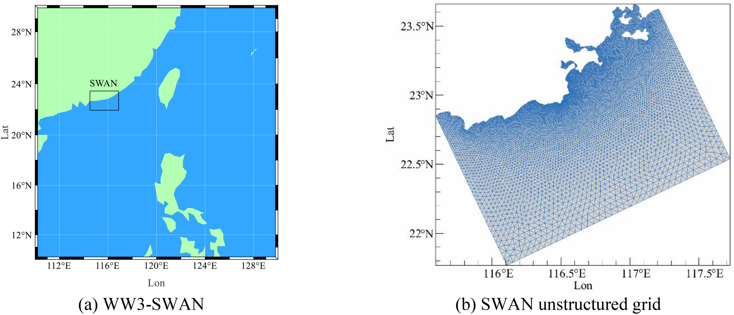
Calculation area of the WW3-SWAN model. (A) WW3-SWAN, (B) SWAN unstructured grid.
The SWAN model was modified and improved by Booij et al. (1996) from Delft University of Technology based on the third-generation wave model WAM. The model discretizes the governing equations using an implicit method, taking into account wave-wave interactions and the breaking effects caused by depth changes during wave propagation, making it effective in simulating the evolution of nearshore waves. The computational range of the SWAN model is from 115.59°E to 117.71°E in longitude and from 21.78°N to 23.66°N in latitude, using an unstructured grid, as shown in Figure 1B. Bathymetric data comes from the GEBCO dataset, wind field data uses ERA5 reanalysis data, and the wave spectrum data at open boundary points is obtained from the wave spectrum output of the WW3 model. The simulation time range is from 00:00:00 on January 1, 2017, to 23:00:00 on December 31, 2021, with an output time interval of one hour.
To verify the accuracy of the WW3-SWAN numerical model, a MARK III Wave Rider instrument was deployed in the waters off the Stone Tablet Mountain Cape, at the coordinate position (22°55.7046′N, 116°31.4034′E), as shown in Figure 2. The Wave Rider instrument has a wave height measurement range of ±20m. The measured data were processed by the instrument’s built-in software, which then statistically generated hourly wave height observation data. The observation period was from 00:00 on April 1, 2021, to 23:00 on November 18, 2021.
Figure 2
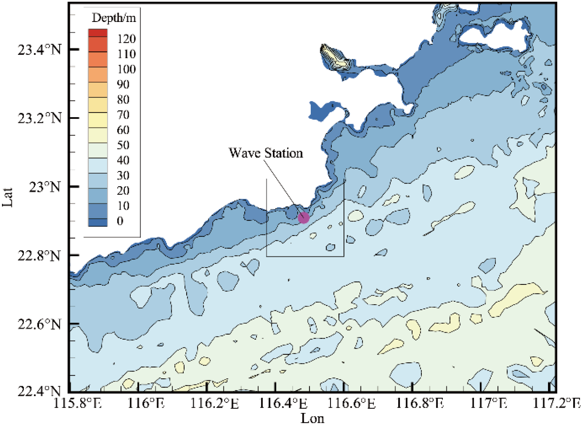
MARK III Wave instrument monitoring position.
2.2 Data validation
Figure 3 shows a comparison between the significant wave heights from the numerical model and the measured values. The significant wave height values from the WW3-SWAN numerical simulation are consistent with the observed values in terms of the overall trend. However, due to the ERA5 reanalysis data underestimating the intensity of typhoons in the Northwest Pacific (Li and Hu, 2021), the numerical simulation slightly underestimates the peak values of the significant wave heights.
Figure 3
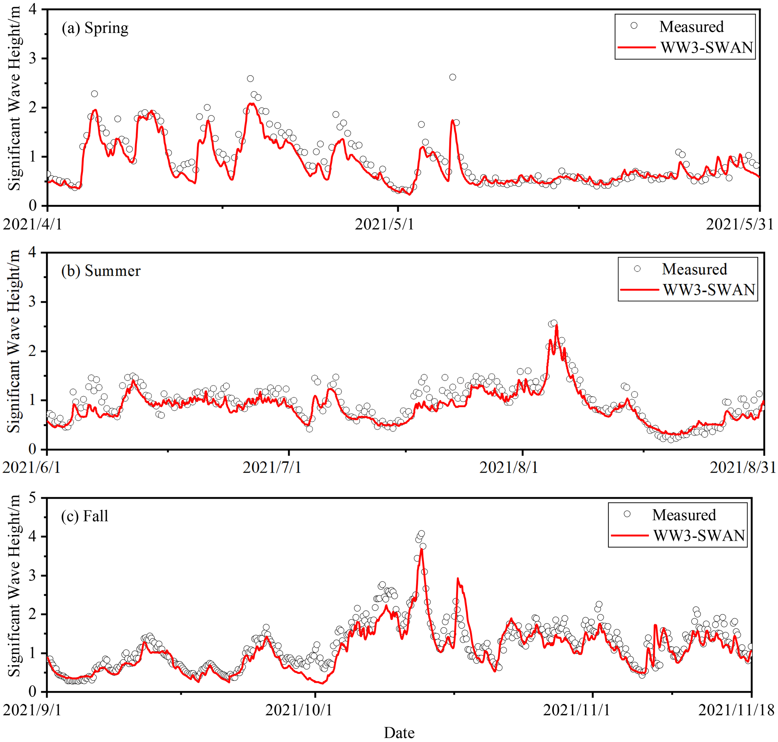
Comparison of WW3-SWAN SWH with the measured value. (A) Spring, (B) Summer, (C) Fall.
Figure 4 shows the situation of some typhoons in the Western Pacific in 2021, with longitude on the horizontal axis, latitude on the vertical axis, and wind speed represented by the color scale. As shown in Figure 4A, during the spring season, Typhoon Surigae formed on April 10, 2021, with wind speeds rapidly increasing from 28 m/s to 60 m/s, and was upgraded to a super typhoon on April 17-18, 2021. The typhoon’s center was located approximately 1,280 km southeast of Manila, Philippines, in the Northwest Pacific Ocean (10.3°N, 131.9°E), with maximum winds near the center reaching 15 on the Beaufort scale (50 m/s). It transitioned into an extratropical cyclone on April 25. At 12:00 on April 18, 2021, the South China Sea was affected by the typhoon, with wind speeds around 10 m/s in the area of the wave monitoring site, leading to higher waves. Therefore, during the typhoon period, the average significant wave height measured in Figure 3A was 1.4m, slightly higher than the numerical simulation value. In May, with no typhoon influence, the average significant wave height at the wave monitoring site was 0.66m, with relatively calm sea conditions, and the numerical simulation values were closer to the measured values at this time.
Figure 4
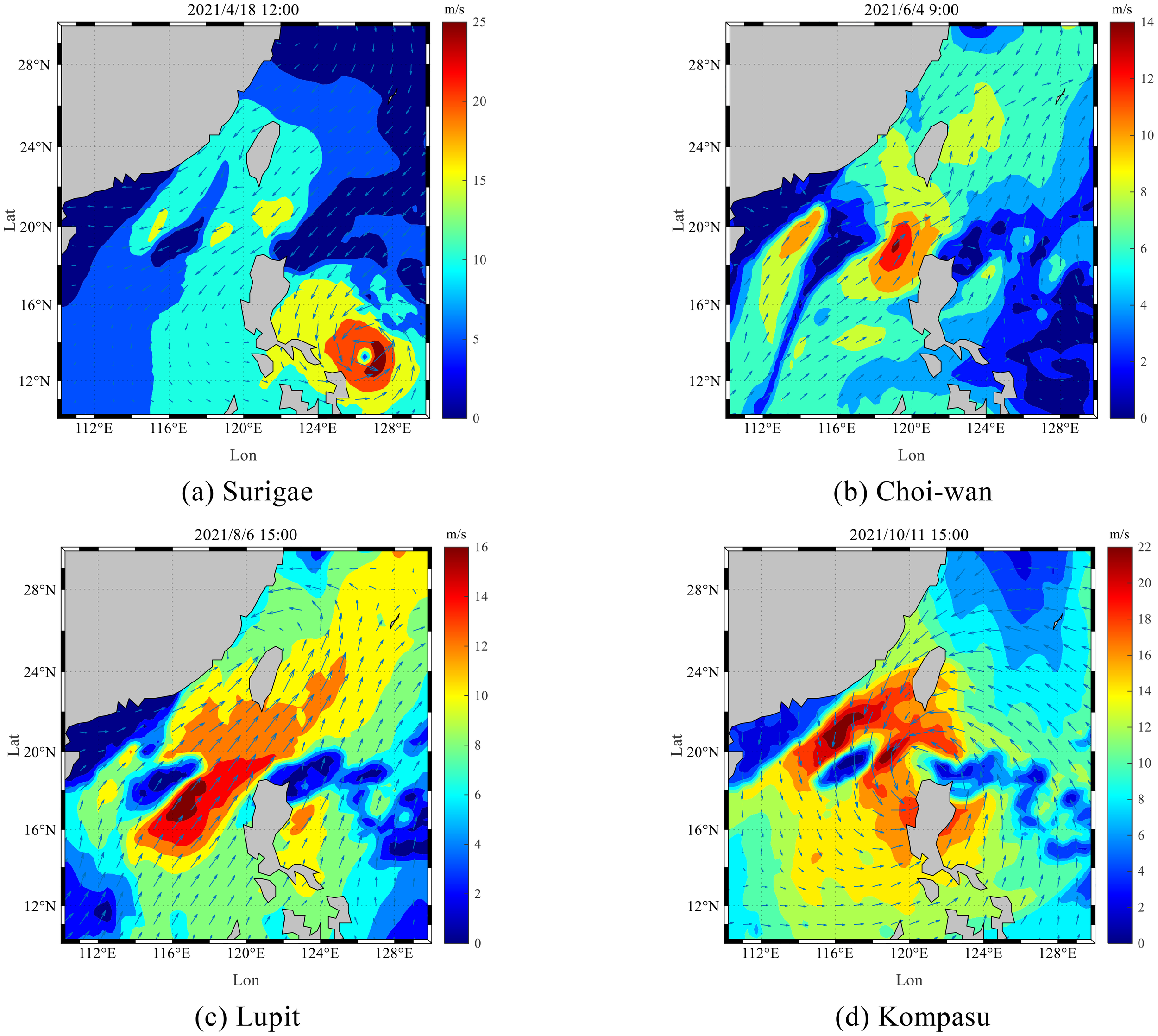
Typhoons in the Western Pacific during 2021. (A) Surigae, (B) Choi-wan, (C) Lupit, (D) Kompasu.
As shown in Figure 4B, during the summer season, Typhoon Choi-Wan entered the South China Sea on June 3, 2021, with maximum sustained winds near the center reaching 65 km/h. At 9:00 on June 4, 2021, wind speeds at the wave monitoring site reached 6-10 m/s, with a peak significant wave height of around 1.5 m. As shown in Figure 4C, Typhoon Lupit formed in Zhanjiang, Guangdong, on August 2, 2021, and gradually approached the coasts of Fujian and Guangdong. By 15:00 on August 6, 2021, wind speeds from Typhoon Lupit along the Fujian-Guangdong coast reached around 10 m/s, causing the wave height at the monitoring site to reach a maximum of approximately 2.5 m. Therefore, during the typhoon periods shown in Figure 4B, the observed values of significant wave height were consistently higher than the values simulated by the numerical model.
As shown in Figure 4D, during the autumn season, Typhoon Kompasu formed in the Philippine Sea on October 8, 2021, and steadily moved westward after entering the South China Sea, with its center approaching the coastal areas of the South China Sea. Therefore, as seen in Figure 3C, the measured wave heights increased significantly during mid-October 2021, while the simulated wave heights were slightly lower.
To further validate the accuracy of the numerical simulation results in this study against the measured data, Mean Absolute Error (MAE), Root Mean Square Error (RMSE), and the coefficient of determination (R²) were used to quantitatively evaluate the accuracy of the numerical results. The calculation formulas are shown in Equations 1–3.
In the formulas, xi represents the numerical simulation values, yi represents the measured values, n is the total number of samples, and and are the mean values of the numerical simulation and measured values, respectively.
To evaluate the WW3-SWAN numerical simulation model, Table 1 uses MAE, RMSE, and R² for a quantitative assessment of model performance. Statistical analysis shows that the WW3-SWAN model performs well across different seasons. The MAE ranges from 0.1413 m to 0.2130 m, indicating that the average deviation between the simulated and observed values is quite small. RMSE, which is more sensitive to larger errors, is slightly higher, ranging from 0.1828 m to 0.2844 m. This is mainly due to the impact of extreme weather conditions like typhoons, which cause deviations in significant wave height at peak values. The R² values are notably high, between 0.7801 and 0.8493, indicating a strong linear relationship between the simulated and observed significant wave heights. The model performs best in the spring, with the highest R² value of 0.8493. In summer and autumn, frequent typhoons lead to reduced accuracy in the numerical simulation. Overall, the WW3-SWAN model reliably reflects the significant wave height in the study area, capturing the magnitude and temporal variation, and can serve as input data for the VMD-CNN-BiLSTM model.
Table 1
| Season | MAE/m | RMSE/m | R2 |
|---|---|---|---|
| Spring (April and May) | 0.1540 | 0.2067 | 0.8493 |
| Summer (June, July and August) | 0.1413 | 0.1828 | 0.7910 |
| Fall (September, October and November) | 0.2130 | 0.2844 | 0.7801 |
Numerical simulation error.
3 Forecasting models
3.1 VMD model
VMD (Variational Mode Decomposition) is an adaptive, fully non-recursive signal processing technique that combines Wiener filtering, Hilbert transform, and the Alternating Direction Method of Multipliers (ADMM). As a non-stationary time series, significant wave height is well-suited for decomposition using VMD. The VMD decomposition process effectively transforms into an optimization process. The two main components of VMD are constructing the variational problem and solving it. Variational modes refer to the modes obtained by solving the variational problem. VMD iteratively searches for the optimal solution of the variational modes, adaptively updating the optimal center frequency and bandwidth for each Intrinsic Mode Function (IMF). VMD redefines the intrinsic mode function, as shown in Equation 4. Compared to other decomposition methods like Empirical Mode Decomposition (EMD) or Wavelet Transform, VMD was chosen for its superior ability to reduce mode mixing and provide more stable component separation under complex wave conditions.
Where k represents the mode number, Ak(t) is the amplitude of the k-th mode, φk(t) is the phase of the k-th mode, and uk(t) is the k-th mode function.
At this point, the variational problem constructed by VMD is shown in Equation 5:
Where uk represents the corresponding mode function, and represents the center frequency of the corresponding mode.
By introducing Lagrange multipliers, the constrained optimization problem above is transformed into an unconstrained problem, as shown in Equation 6:
Where α represents the variance regularization parameter, and λ represents the Lagrange multiplier.
To solve this problem, the Alternating Direction Method of Multipliers (ADMM) is used. The specific solving steps are as follows:
-
Initialize , , and the iteration number n.
-
Increase the variable n to 1 and enter the loop.
-
Update the variables according to Equation 7 until the number of iterations exceeds k, then stop updating:
-
Update the Lagrange multipliers λ
-
If the condition of Equation 9 is met, the loop ends; if not, return to step 2.
By constructing and solving the variational problem, VMD can effectively decompose non-stationary data. However, the number of modes after VMD decomposition needs to be manually selected. Multiple tests are required to find the most appropriate number of modes.
3.2 CNN model
CNN are an effective deep learning model widely used for feature extraction in image processing and spatio-temporal data. Through mechanisms like local receptive fields and weight sharing, CNNs can effectively capture local spatial features in the data. In this forecasting model, CNN is used to extract the spatial features of wind fields and wave heights, which will serve as inputs for subsequent time series modeling. CNN architecture is constructed by stacking three main types of layers: convolutional layers, pooling layers, and fully connected (FC) layers. Each convolutional layer contains a set of learnable filters, which aim to automatically extract local features from the input matrix. These filters perform convolution operations based on two important concepts: weight sharing and local connections, which help reduce computational complexity and enhance model performance. The pooling layer follows the convolutional layer, performing down-sampling. A notable feature of the pooling layer is its ability to reduce the dimensionality of feature maps, thus preventing overfitting. Typically, FC layers are used in the final layers of CNN architecture, and their role is to learn nonlinear combinations of features extracted by convolutional layers, generating the final output. Since wave height and wind field data usually exhibit significant spatio-temporal dependencies, CNN can effectively extract local features and patterns from this data through its receptive fields. Therefore, CNN is selected to extract features from wind fields and wave heights in this study.
Figure 5 illustrates the specific process of wind field and wave height data processed through a one-dimensional Convolutional Neural Network (1D-CNN). The input data, representing a sample at a certain time from the dataset, is preprocessed and fed into the convolutional layer of the CNN in sequence form. In the convolutional layer, multiple filters (also known as convolutional kernels) slide over the input sequence, extracting local temporal features through local connectivity and weight sharing. After the convolution operation, the data moves to the pooling layer for downsampling. By selecting the maximum value (max pooling) or the average value (average pooling) within a window, the dimensionality of the feature map is reduced. This not only decreases the computational complexity of the model but also effectively prevents overfitting. After processing by the pooling layer, the dimensionality of the feature map is significantly reduced, preserving key features while lowering computation costs. Finally, these processed feature maps are flattened into a one-dimensional vector, which serves as input for subsequent fully connected layers or other models (such as LSTM or BiLSTM) for the final prediction task.
Figure 5
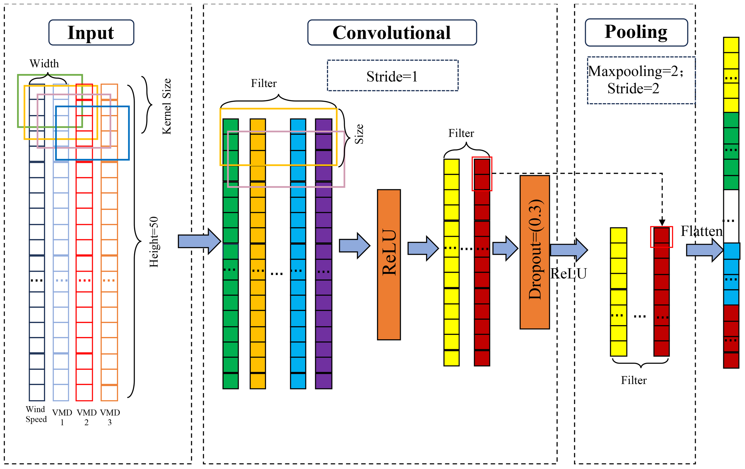
Flow chart of the one-dimensional CNN model.
3.3 BiLSTM model
Additionally, since the current wave height is not only related to the current wind field conditions but also influenced by historical wind field and wave height changes, traditional neural networks struggle to capture this long-term dependency. LSTM, with its special architecture, can effectively retain and utilize information from long-term time series, allowing it to capture complex temporal patterns in the data. Moreover, LSTM can solve the vanishing gradient problem found in conventional Recurrent Neural Networks (RNN), making it more stable and accurate in predicting long sequences. Therefore, in wave height forecasting tasks, LSTM becomes a natural choice to better model the temporal dependency and dynamic changes in the data.
A typical LSTM unit contains three types of gates: the input gate it, forget gate ft, and output gate ot, as shown in Figure 6. In each gate, the state of the memory cell is controlled through element-wise multiplication and the Sigmoid function. The inputs to the LSTM model are the input data at the current state xt and the output of the hidden state from the previous layer ht-1.
Figure 6
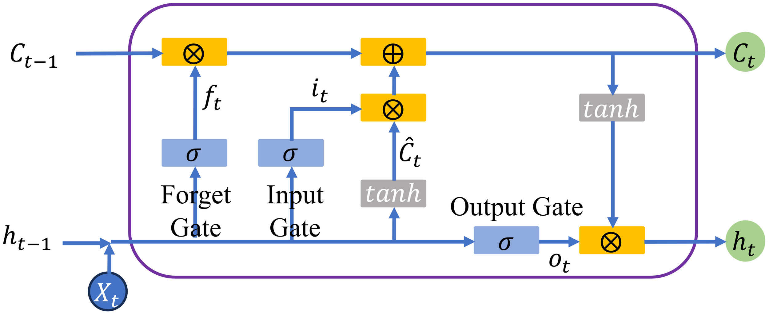
LSTM structure diagram.
The input data first passes through the forget gate, which determines which information should be discarded or retained. The equation for the forget gate is as follows:
Here, σ represents the Sigmoid activation function, and Wf and bf represent the weights and biases of the forget gate, respectively. The current input xt and the previous hidden state ht-1 are fed into the Sigmoid function. By transforming values between 0 and 1, the forget gate determines which information needs to be updated, where 0 represents unimportant information and 1 represents important information.
Next, the data passes through the input gate, with the calculation formula as follows:
Then, the current input xt and the hidden state ht-1 are fed into the hyperbolic tangent function (tanh). At this point, the cell state is calculated and updated to the new cell state. The formula is as follows:
Here, tanh is the hyperbolic tangent activation function, and ⊙ denotes the element-wise multiplication operation, with Ct being the new cell state.
Finally, the output gate selects the next hidden state. The new cell state Ct and the new hidden state ht are passed to the next time step. The formula for the output gate is as follows:
A unidirectional LSTM can only process information flow in one direction, whereas a bidirectional LSTM (BiLSTM) enhances the model’s ability to understand wave height and wind field temporal evolution by analyzing both forward and backward information in parallel. BiLSTM consists of two LSTM layers operating in opposite directions, as illustrated in Figure 7. The horizontal dashed line represents the time axis flow of the time series data, while the vertical slanted lines depict the information transmission paths between network layers.
Figure 7
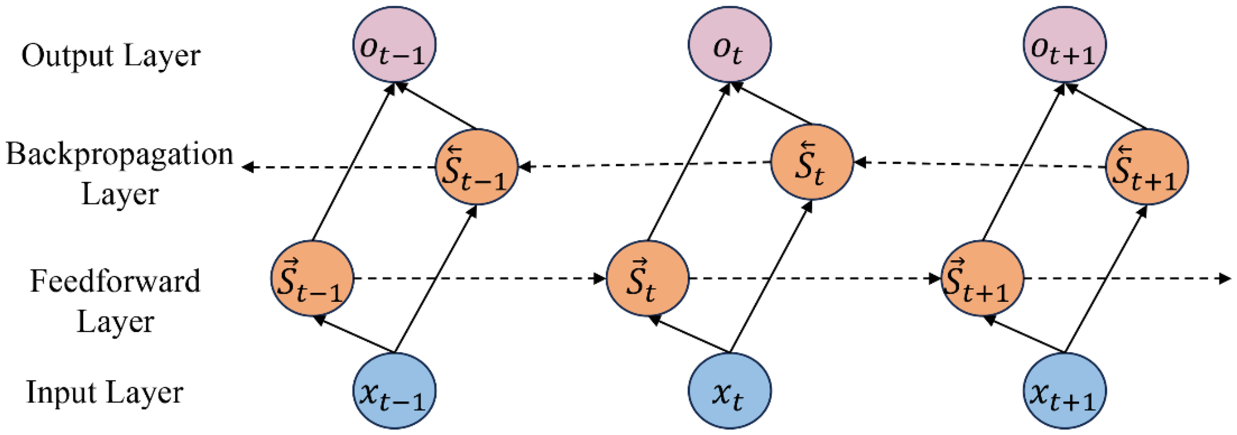
Bi-LSTM structure diagram.
3.4 VMD-CNN-BiLSTM model
The VMD-CNN-BiLSTM model is shown in Figure 8. VMD decomposes the wave height data into several Intrinsic Mode Functions (IMFs), breaking down the non-stationary wave height time series into relatively stationary subcomponents. The CNN network extracts local features from wind speed and IMFs, while the BiLSTM network models the wave time series data to accurately predict future wave heights. The detailed process is as follows:
-
Data collection and preprocessing: Gather datasets that include wind field and wave height data, and perform preprocessing steps like data cleaning and normalization to ensure the data is suitable for model training.
-
Dataset splitting: Divide the dataset into training and testing sets to ensure that the training set has enough data for model learning, while the testing set is used to evaluate the model’s performance.
-
VMD decomposition: Apply VMD to decompose the wave height data. The original wave height data is decomposed into several IMFs, each representing different frequency components of the data. This decomposition helps CNN better extract multi-scale features from the wave data.
-
Feature extraction via CNN: Apply a multi-layer Convolutional Neural Network (CNN) to process the input data, extracting spatial features from the wind field and IMFs. The CNN layers help identify patterns and relationships between spatial data points that affect wave heights.
-
Temporal feature extraction via Bi-LSTM: Pass the spatial features extracted by CNN into a bidirectional Long Short-Term Memory network (Bi-LSTM), which extracts the temporal features from the data. The Bi-LSTM layer captures time dependencies, allowing the model to account for how event sequences and timings affect wave height variations.
-
Feature merging and fully connected layers: Merge the features extracted by CNN and Bi-LSTM and pass the merged features through fully connected layers for learning.
-
Output layer: After the last fully connected layer, a single neuron output layer is used to produce the final wave height prediction.
Figure 8
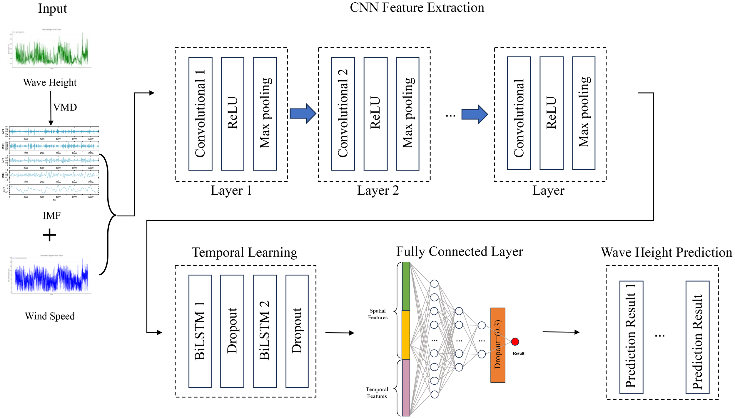
CNN-BiLSTM Flowchart.
4 Wave height prediction
The southeastern seas of China are influenced by the monsoon climate, with prevailing northerly winds in winter and predominantly southerly winds in summer. Waves, influenced by these wind fields, exhibit a seasonal distribution characterized by lower effective wave heights in spring and summer, and higher effective wave heights in autumn and winter (Qiu et al., 2019). As shown in Figure 9, during spring and summer, the effective wave heights in the southeastern sea area range mainly from 0.2 to 1.2 meters. In autumn, the effective wave heights significantly increase, with the mean value ranging from 0.6 to 1.6 meters. In winter, the mean wave height increases further, with the maximum average reaching approximately 2.3 meters. Therefore, when using the VMD-CNN-BiLSTM model to predict effective wave heights, it is necessary to predict the wave heights for each season separately.
Figure 9
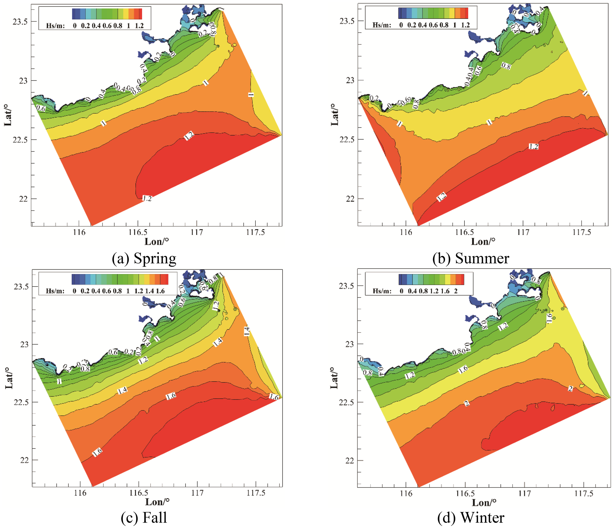
Seasonal distribution of significant wave heights over five years. (A) Spring, (B) Summer, (C) Fall, (D) Winter.
4.1 VMD decomposition
Before being input into the prediction model, the wave height dataset was normalized to a range between 0 and 1, which accelerates the model’s convergence and improves prediction accuracy.
Due to the influence of the monsoon climate and typhoons in this sea area, the effective wave height sequence fluctuates greatly, requiring data processing. This paper uses Variational Mode Decomposition (VMD) to decompose the original sequences of wind fields and effective wave heights into several relatively smooth components. Taking the spring period from 2017 to 2021 as an example, with a data time interval of 1 hour, the VMD decomposition results are shown in Figure 10.
Figure 10
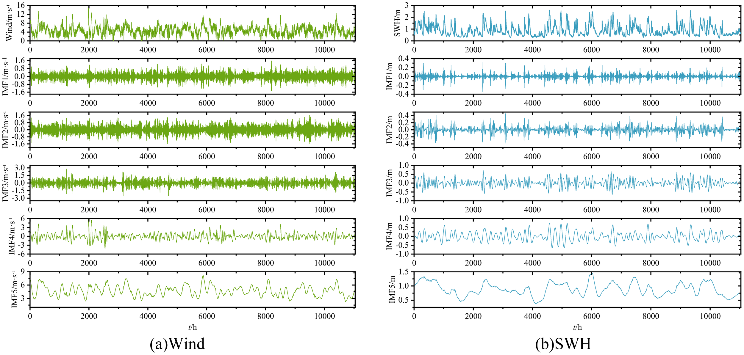
VMD decomposition of significant wave height sequence. (A) Wind, (B) SWH.
From the decomposition, we can observe that the wind field (Figure 10A) and the effective wave height (Figure 10B) sequences are decomposed into five components (IMF1 to IMF5), transitioning from high-frequency to low-frequency components.
To compare the impact of VMD decomposition of wind fields and effective wave heights on wave height prediction, two cases were designed: Case 1 includes seven vectors, namely the wind field, IMF1 to IMF5 of the effective wave height, and the original effective wave height; Case 2 includes 12 vectors, specifically IMF1 to IMF5 of the wind field, the wind field, IMF1 to IMF5 of the effective wave height, and the original effective wave height.
According to the data in Table 2, the prediction results of Case 1 and Case 2 show significant differences across different seasons. In all seasons, the errors in Case 1 are generally smaller than those in Case 2, indicating that decomposing only the effective wave height better captures its intrinsic features, while introducing the IMF components of the wind field increases the model’s complexity, leading to greater errors. Notably, the computation time for Case 1 is significantly shorter than for Case 2, especially in winter, where the CPU time for Case 2 is more than 10 times that of Case 1. This further suggests that introducing the IMF components of the wind field not only increases the model’s computational complexity but also significantly prolongs the computation time. Therefore, in the subsequent predictions, to simplify the computation and improve model efficiency, only the effective wave height data, which has a more significant impact on the predictions, will be decomposed.
Table 2
| Season | Evaluation | Case 1 | Case 2 |
|---|---|---|---|
| Spring | MAE/m | 0.0147 | 0.0214 |
| RMSE/m | 0.0202 | 0.0285 | |
| R2 | 0.9981 | 0.9962 | |
| CPU time/s | 308 | 3544 | |
| Summer | MAE/m | 0.0112 | 0.0197 |
| RMSE/m | 0.0147 | 0.0258 | |
| R2 | 0.9980 | 0.9938 | |
| CPU time/s | 332 | 3345 | |
| Fall | MAE/m | 0.0228 | 0.0340 |
| RMSE/m | 0.0306 | 0.0491 | |
| R2 | 0.9971 | 0.9925 | |
| CPU time/s | 311 | 3597 | |
| Winter | MAE/m | 0.0197 | 0.0273 |
| RMSE/m | 0.0268 | 0.0363 | |
| R2 | 0.9977 | 0.9958 | |
| CPU time/s | 254 | 5098 |
VMD decomposition signal impact.
4.2 Univariate prediction
This experiment used data from spring, summer, autumn, and winter between 2017 and 2021 as model driving data, with data from 2017 to 2020 used as the training set and data from 2021 as the test set. In the univariate model, only significant wave height is used as the input parameter for the BiLSTM, CNN-BiLSTM, and VMD-CNN-BiLSTM models.
Figure 11 compares the univariate predictions of BiLSTM, CNN-BiLSTM, and VMD-CNN-BiLSTM models with the WW3-SWAN simulation values. As shown in Figure 11, the bidirectional LSTM (BiLSTM) is capable of considering both past and future information and performs well in predicting the overall trend, especially in periods with smaller fluctuations. However, in regions of sharp changes in wave peaks and troughs (as indicated by the black boxes in Figure 11), BiLSTM shows significant errors compared to the WW3-SWAN values. This may be due to BiLSTM’s tendency to over-smooth the predictions during periods of sharp fluctuations. In contrast, the CNN-BiLSTM model is more effective at capturing the short-term fluctuations of wave peaks, particularly in areas of peak changes, outperforming BiLSTM. However, CNN-BiLSTM is less effective at capturing troughs, possibly due to limitations in its ability to extract local features. By decomposing the significant wave height data using VMD, the model can effectively extract important frequency components, and combined with CNN’s ability to extract local features, it significantly improves prediction accuracy in areas of sharp changes in wave peaks and troughs. Overall, the VMD-CNN-BiLSTM model performs best in capturing changes in wave peaks and troughs.
Figure 11
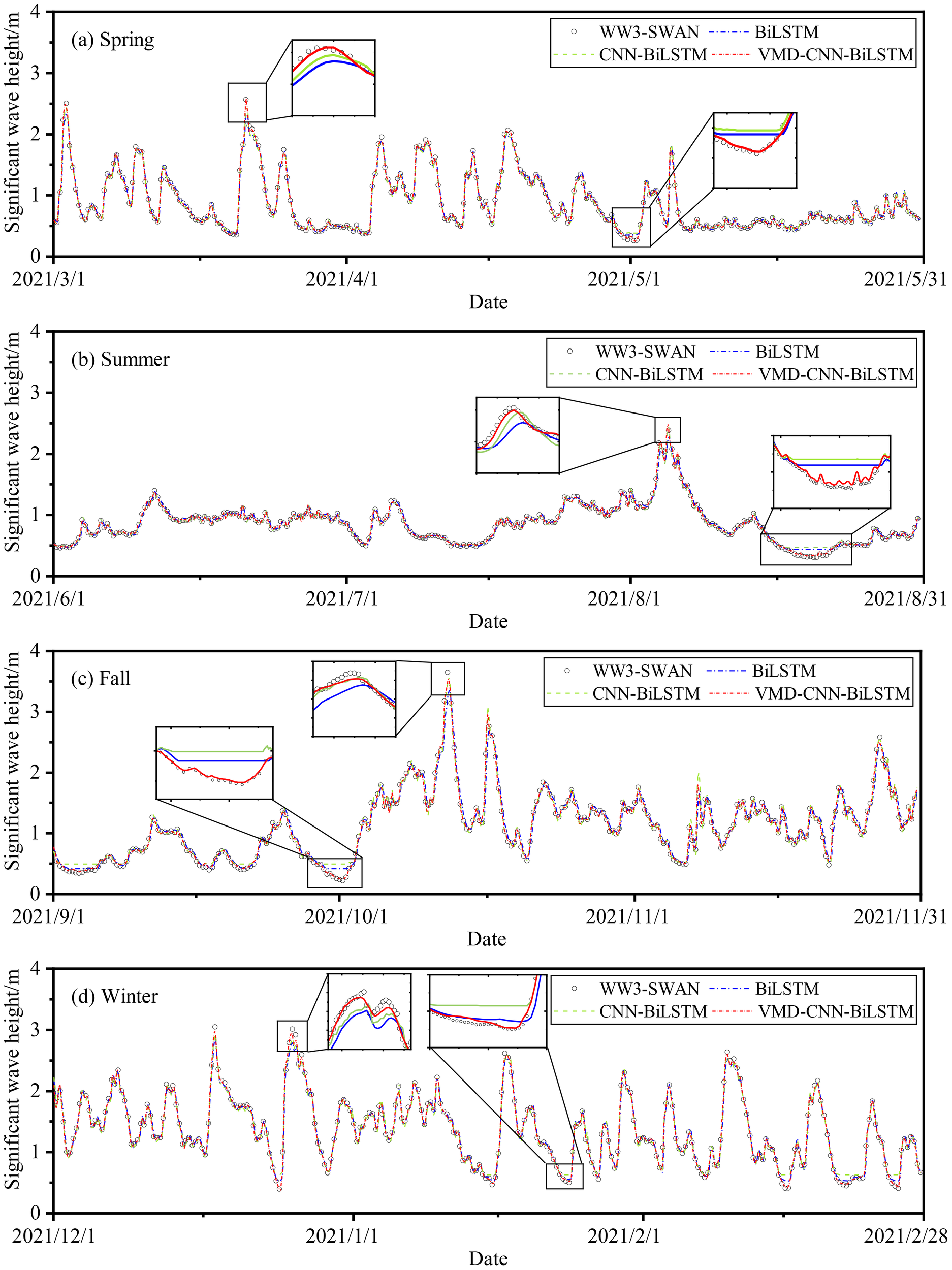
The WW3-SWAN simulated and predicted values of SWH of univariate. (A) Spring, (B) Summer, (C) Fall, (D) Winter.
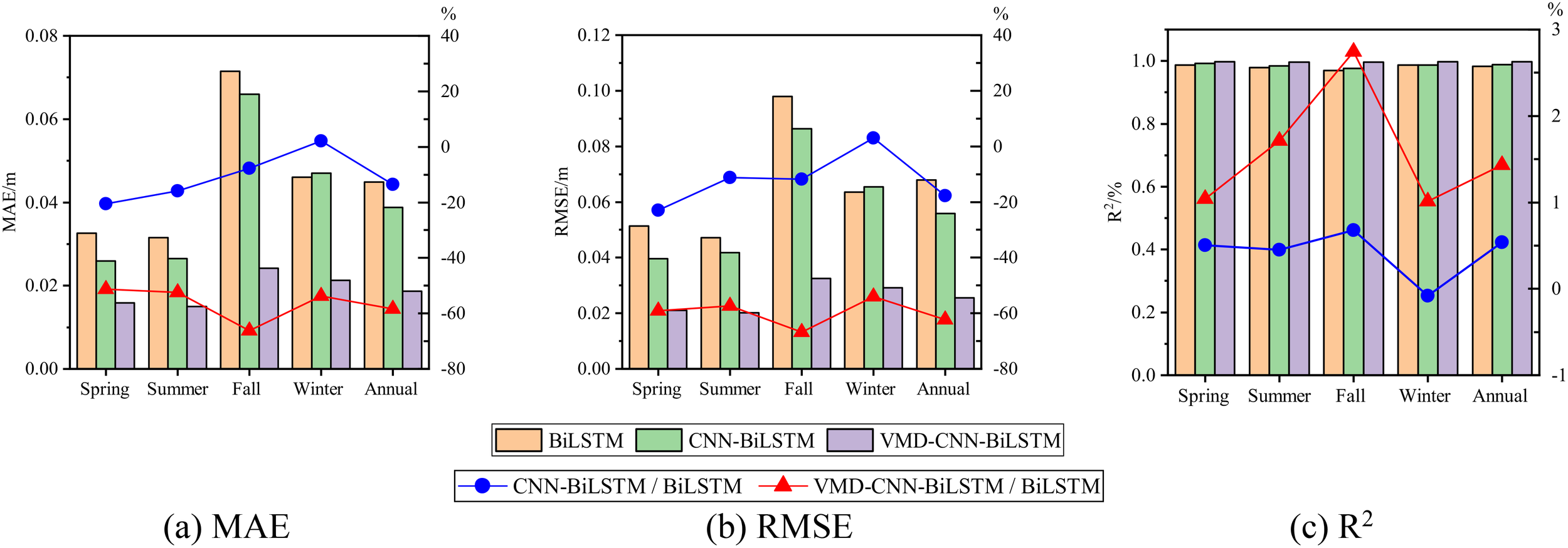
Figure 12 and Table 3 compare the error metrics of the three models (BiLSTM, CNN-BiLSTM, and VMD-CNN-BiLSTM) in univariate significant wave height prediction, including mean absolute error (MAE), root mean square error (RMSE), and coefficient of determination (R²). The left y-axis of Figure 11 represents the specific values of MAE, RMSE, and R² for each model, while the right y-axis shows the relative values of each model compared to BiLSTM. Negative values of MAE and RMSE indicate that the model performs better than BiLSTM, while positive values indicate poorer performance; for R², larger positive values indicate better prediction accuracy. The results show that the VMD-CNN-BiLSTM model’s error is significantly lower than the other two models, especially in regions of sharp changes in wave peaks and troughs. Across all seasons, the VMD-CNN-BiLSTM model demonstrates the best prediction performance, particularly in the autumn and winter seasons, where complex wave height changes caused by typhoons and strong monsoons are present. For example, in the spring season, the MAE of the VMD-CNN-BiLSTM is 0.0159 meters, a 51.23% reduction compared to BiLSTM; across the entire year, the RMSE of the VMD-CNN-BiLSTM is 0.0256 meters, a 62.30% reduction compared to BiLSTM. Furthermore, the R² of the VMD-CNN-BiLSTM is the highest across all seasons and in annual statistics, reaching 0.9979 in the spring, a 1.04% improvement compared to BiLSTM. This indicates that the VMD-CNN-BiLSTM model has a stronger correlation between the predicted results and the actual observations, reflecting the actual wave height changes more accurately. Therefore, the MAE and RMSE of the VMD-CNN-BiLSTM model are significantly lower than those of other models across different seasons, indicating superior performance in capturing wave peaks and troughs. The higher R² value further demonstrates the model’s advantage in trend prediction, particularly in handling complex fluctuations.
Figure 12
The WW3-SWAN simulated and predicted values of SWH of multivariate. (A) Spring, (B) Summer, (C) Fall, (D) Winter.
Table 3
| Season | Error | BiLSTM | CNN-BiLSTM | VMD-CNN-BiLSTM |
|---|---|---|---|---|
| Spring | MAE/m | 0.0326 | 0.0259 (-20.55) | 0.0159 (-51.23) |
| RMSE/m | 0.0514 | 0.0396 (-22.96) | 0.0210 (-59.14) | |
| R2/% | 0.9876 | 0.9926 (0.51) | 0.9979 (1.04) | |
| Summer | MAE/m | 0.0315 | 0.0265 (-15.87) | 0.0150 (-52.38) |
| RMSE/m | 0.0471 | 0.0418 (-11.25) | 0.0201 (-57.32) | |
| R2/% | 0.9794 | 0.9838 (0.45) | 0.9962 (1.72) | |
| Fall | MAE/m | 0.0715 | 0.0660 (-7.69) | 0.0242 (-66.15) |
| RMSE/m | 0.0979 | 0.0863 (-11.85) | 0.0325 (-66.80) | |
| R2/% | 0.9701 | 0.9767 (0.68) | 0.9967 (2.74) | |
| Winter | MAE/m | 0.0460 | 0.0470 (2.17) | 0.0213 (-53.70) |
| RMSE/m | 0.0635 | 0.0654 (2.99) | 0.0292 (-54.02) | |
| R2/% | 0.9873 | 0.9865 (-0.08) | 0.9973 (1.01) | |
| Annual | MAE/m | 0.0449 | 0.0388 (-13.58) | 0.0187 (-58.35) |
| RMSE/m | 0.0679 | 0.0558 (-17.82) | 0.0256 (-62.30) | |
| R2/% | 0.9836 | 0.9889 (0.54) | 0.9977 (1.43) |
Statistics of univariate SWH prediction error.
The values in parentheses represent the percentage improvement of each model’s performance indicators compared to BiLSTM.
4.3 Multivariate forecasting
Due to the influence of the monsoon climate in the region, this study conducted a multivariate prediction research to further improve prediction accuracy. In the experiment, both wind speed and significant wave height were used as parameters for the prediction model, considering the impact of the wind field. Similarly, data from spring, summer, autumn, and winter between 2017 and 2021 were used as model driving data, with data from 2017 to 2020 as the training set and data from 2021 as the test set.
Figure 13 presents the comparison curves of multivariate predictions from BiLSTM, CNN-BiLSTM, and VMD-CNN-BiLSTM models with WW3-SWAN simulation values. The figure shows that the monsoon climate significantly affects the wind field and wave height variations in the Southeast China Sea, especially in summer and autumn, where the frequent occurrence of typhoons exacerbates the complexity of wave height changes. Therefore, considering multivariate factors such as the wind field is crucial for improving the accuracy of wave height predictions. Spring is a transitional period from the winter to summer wind directions, with complex wind field changes, especially during the impact of typhoon “Shuriki,” where wind speed and wave height fluctuations significantly increase. Figure 13A shows that, compared to univariate predictions, multivariate predictions more accurately capture the overall trend of spring wave heights. Notably, the VMD-CNN-BiLSTM model, by effectively integrating instantaneous changes in the wind field, can accurately predict wave peak and trough changes, with its prediction curve highly aligning with WW3-SWAN simulation values, demonstrating high prediction accuracy. In summer, the prevailing southeast monsoon leads to a relatively stable wind field. Figure 13B indicates that, compared to univariate predictions, the VMD-CNN-BiLSTM model performs particularly well when considering wind field factors, with its prediction curve closely matching the WW3-SWAN simulation values, especially during August 17 to August 20, when VMD-CNN-BiLSTM accurately captures the characteristics of wave troughs. Autumn is a transitional period from summer to winter winds, with frequent typhoons and significant wave height changes. Figure 13C shows that the VMD-CNN-BiLSTM model better utilizes the intense changes in wind field data to accurately capture extreme wave peak values. The model performs excellently under extreme weather conditions such as typhoons, with its prediction curve closest to the WW3-SWAN simulation values. In winter, the Northeast monsoon prevails in the Southeast China Sea, with strong winds and long durations, resulting in higher overall wave height levels and frequent fluctuations. Figure 13D shows that in winter, the VMD-CNN-BiLSTM model effectively captures the overall trend and local fluctuations of wave heights, with its prediction curve highly consistent with the WW3-SWAN simulation values, demonstrating the best prediction performance.
Figure 13
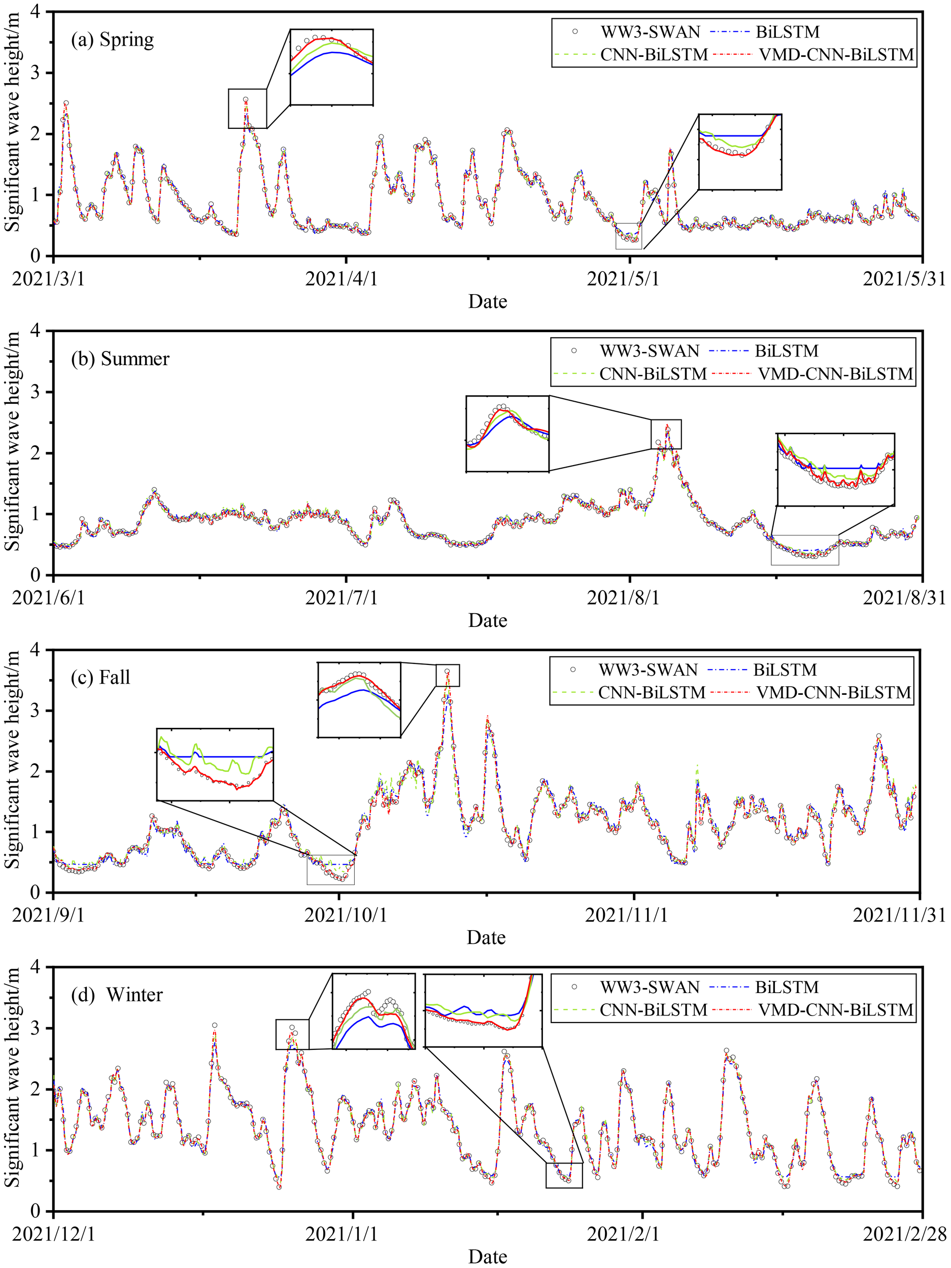
The WW3-SWAN simulated and predicted values of SWH of multivariate.
Figure 14 and Table 4 show the error performance of multivariate significant wave height prediction models (BiLSTM, CNN-BiLSTM, and VMD-CNN-BiLSTM) in different seasons and annual statistics, including mean absolute error (MAE), root mean square error (RMSE), and coefficient of determination (R²), as well as the ratios of each model relative to BiLSTM. The influence of the Southeast China Sea monsoon climate and typhoons was considered to evaluate each model’s performance under complex meteorological conditions. The data in Figure 14 and Table 3 indicate that, within the same season, the VMD-CNN-BiLSTM model has significantly lower errors than the other two models. Particularly, after considering multivariate factors such as the wind field, the prediction performance of VMD-CNN-BiLSTM has significantly improved. Seasonal differences in prediction performance indicate that VMD-CNN-BiLSTM performs exceptionally well in autumn and winter, accurately capturing the drastic wave height changes brought by typhoons and strong monsoons. VMD-CNN-BiLSTM shows optimal performance in MAE and RMSE across all seasons, indicating that this model significantly outperforms BiLSTM and CNN-BiLSTM in multivariate prediction accuracy. For example, in spring, the MAE of VMD-CNN-BiLSTM is 0.0147 meters, a 51.48% reduction compared to BiLSTM; in annual statistics, the RMSE of VMD-CNN-BiLSTM is 0.0244 meters, a 61.81% reduction compared to BiLSTM. Additionally, the R² value of VMD-CNN-BiLSTM is the highest across all seasons and annual statistics, reaching 0.9981 in spring, a 0.79% improvement compared to BiLSTM, indicating stronger correlation and consistency in multivariate predictions. The inclusion of wind speed significantly improved the predictive performance of the VMD-CNN-BiLSTM model, particularly under complex meteorological conditions in autumn and winter, resulting in lower MAE and RMSE, as well as higher R². This indicates that the model is more effective at capturing the complex relationship between wind fields and wave heights, thereby enhancing the accuracy and stability of wave height predictions.
Figure 14
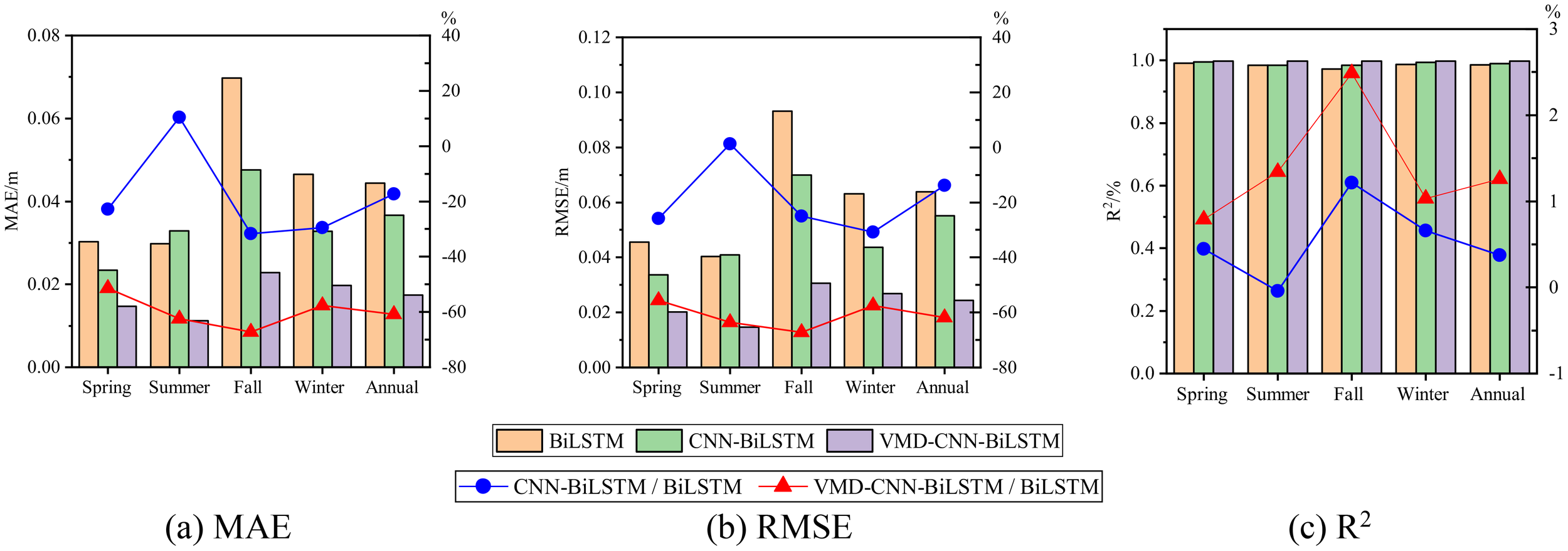
Multivariate significant wave height prediction error, (A) MAE, (B) RMSE, (C) R2.
Table 4
| Season | Evaluation | BiLSTM | CNN-BiLSTM | VMD-CNN-BiLSTM |
|---|---|---|---|---|
| Spring | MAE/m | 0.0303 | 0.0234 (-22.77) | 0.0147 (-51.48) |
| RMSE/m | 0.0455 | 0.0337 (-25.93) | 0.0202 (-55.60) | |
| R2/% | 0.9903 | 0.9947 (0.44) | 0.9981 (0.79) | |
| Summer | MAE/m | 0.0298 | 0.0329 (10.40) | 0.0112 (-62.42) |
| RMSE/m | 0.0404 | 0.0409 (1.24) | 0.0147 (-63.61) | |
| R2/% | 0.9848 | 0.9844 (-0.04) | 0.9980 (1.34) | |
| Fall | MAE/m | 0.0697 | 0.0476 (-31.71) | 0.0228 (-67.29) |
| RMSE/m | 0.0932 | 0.0699 (-25.00) | 0.0306 (-67.17) | |
| R2/% | 0.9729 | 0.9847 (1.21) | 0.9971 (2.49) | |
| Winter | MAE/m | 0.0465 | 0.0328 (-29.46) | 0.0197 (-57.63) |
| RMSE/m | 0.0631 | 0.0437 (-30.74) | 0.0268 (-57.53) | |
| R2/% | 0.9875 | 0.9940 (0.66) | 0.9977 (1.03) | |
| Annual | MAE/m | 0.0444 | 0.0367 (-17.34) | 0.0174 (-60.81) |
| RMSE/m | 0.0639 | 0.0551 (-13.77) | 0.0244 (-61.81) | |
| R2/% | 0.9855 | 0.9892 (0.38) | 0.9979 (1.26) |
Statistics of multivariate SWH prediction error.
The values in parentheses represent the percentage improvement of each model’s performance indicators compared to BiLSTM.
5 Conclusion
This study employs Variational Mode Decomposition (VMD) to extract significant features of significant wave height as intrinsic mode functions, combines Convolutional Neural Networks (CNN) to capture complex internal mappings of wind and waves, and integrates with Bidirectional Long Short-Term Memory (BiLSTM) networks to establish the VMD-CNN-BiLSTM model. The research focuses on the Southeast China Sea, with datasets provided by ECMWF and WW3-SWAN simulations. The case study and prediction results lead to the following conclusions:
-
Compared to models like BiLSTM and CNN-BiLSTM, the VMD-CNN-BiLSTM model is able to more accurately capture the peaks and smooth trends of wave height, resulting in higher prediction accuracy.
-
After incorporating wind field data, the MAE and RMSE of each prediction model decrease. Specifically, the VMD-CNN-BiLSTM model’s MAE and RMSE are reduced to 0.0174 meters and 0.0244 meters respectively for annual statistics, with the coefficient of determination (R²) increasing to 0.9979, outperforming other prediction models.
-
The VMD-CNN-BiLSTM model exhibits optimal prediction performance across all four seasons, particularly in winter under the influence of strong northeast monsoons and during summer and autumn when typhoons and extreme weather events occur. Its prediction performance significantly surpasses that of BiLSTM and CNN-BiLSTM models, demonstrating the model’s excellent adaptability to complex sea conditions.
Statements
Data availability statement
The original contributions presented in the study are included in the article/supplementary material. Further inquiries can be directed to the corresponding author.
Author contributions
WS: Data curation, Methodology, Visualization, Writing – original draft. ZY: Conceptualization, Methodology, Writing – review & editing. YZ: Formal analysis, Validation, Writing – review & editing. XW: Project administration, Supervision, Writing – review & editing.
Funding
The author(s) declare that no financial support was received for the research, authorship, and/or publication of this article.
Acknowledgments
We are very grateful to ECMWF for providing the wind field data, GEBCO for providing the bathymetry data, and CCCC-Fourth Harbor Engineering Institute Co., Ltd. for providing the wave buoy data.
Conflict of interest
Authors WS and YZ were employed by company CCCC Fourth Harbor Engineering Institute Co., Ltd. Authors ZY and XW were employed by companies CCCC Fourth Harbor Engineering Institute Co., Ltd. and CCCC.
Generative AI statement
The author(s) declare that no Generative AI was used in the creation of this manuscript.
Publisher’s note
All claims expressed in this article are solely those of the authors and do not necessarily represent those of their affiliated organizations, or those of the publisher, the editors and the reviewers. Any product that may be evaluated in this article, or claim that may be made by its manufacturer, is not guaranteed or endorsed by the publisher.
References
1
Abed-Elmdoust A. Kerachian R. (2012). Wave height prediction using the rough set theory. Ocean Eng.54, 244–250. doi: 10.1016/j.oceaneng.2012.07.020
2
Ahmed A. A. M. Jui S. J. J. Al-Musaylh M. S. Raj N. Saha R. Deo R. C. et al . (2024). Hybrid deep learning model for wave height prediction in Australia’s wave energy region. Appl. Soft Comput.150, 111003. doi: 10.1016/j.asoc.2023.111003
3
Berbíc J. Ocvirk E. Carevíc D. Loňcar G. (2017). Application of neural networks and support vector machine for significant wave height prediction. Oceanologia59.3, 331–349. doi: 10.1016/j.oceano.2017.03.007
4
Booij N. Holthuijsen L. Ris R. (1996). The “Swan” Wave model for shallow water. Coast. Eng.1996, 668–676. doi: 10.1061/9780784402429.0
5
Bottcher A. B. Whiteley B. J. James A. I. Hiscock J. G. (2012). Watershed assessment model (WAM): model use, calibration, and validation. Trans. ASABE55.4, 1367–1383. doi: 10.13031/2013.42248
6
Deo M. C. Jha A. Chaphekar A. S. Ravikant K. (2001). Neural networks for wave forecasting. Ocean Eng.28.7, 889–898. doi: 10.1016/S0029-8018(00)00027-5
7
Fan C. Wang X. Zhang X. Gao D. (2019). A newly developed ocean significant wave height retrieval method from Envisat AS-AR wave mode imagery. Acta Oceanologica Sin.38, 120–127. doi: 10.1007/s13131-019-1480-2
8
Gers F. A. Schraudolph N. N. Schmidhuber J. (2002). Learning precise timing with LSTM recurrent networks. J. Mach. Learn. Res.3, 115–143.
9
Hao P. Li S. Gao Y. (2023). Significant wave height prediction based on deep learning in the South China Sea. Front. Mar. Sci.9, 1113788. doi: 10.3389/fmars.2022.1113788
10
Kaloop M. R. Kumar D. Zarzoura F. Roy B. Hu J. W. (2020). A wavelet—Particle swarm optimization—Extreme learning machine hybrid modeling for significant wave height prediction. Ocean Eng.213, 107777. doi: 10.1016/j.oceaneng.2020.107777
11
Li J. Hu Y. (2021). Assessment of typhoons in ERA-Interim and ERA-5 reanalysis datasets. Hydro-Science Eng. (2021), 62–69. doi: 10.12170/20200222001
12
Liang B. Gao H. Shao Z. (2019). Characteristics of global waves based on the third-generation wave model SWAN. Mar. Structures64, 35–53. doi: 10.1016/j.marstruc.2018.10.011
13
Liu Q. Rogers W. E. Babanin A. V. Young I. R. Romero L. Zieger S. et al . (2019). Observation-based source terms in the third-generation wave model WAVEWATCH III: Updates and verification. J. Phys. Oceanogr.49, 489–517. doi: 10.1175/JPO-D-18-0137.1
14
Lixiang S. Yunyue C. Zonghui M. Songgui C. (2023). Research on wave height prediction in Longkou sea area based on Attention-LSTM network. J. Waterway Harbor44, 196–201. doi: 10.3969/j.issn.1005-8443.2023.02.006
15
Mentaschi L. Besio G. Cassola F. Mazzino A. (2015). Performance evaluation of wavewatch III in the Mediterranean sea. Ocean Model.90, 82–94. doi: 10.1016/j.ocemod.2015.04.003
16
Mikolov T. Kombrink S. Burget L. Cernocky J. Khudanpur S. (2021). “Extensions of recurrent neural network language model,” in 2011 IEEE international conference on acoustics, speech and signal processing (ICASSP). 5528–5531 (Piscataway, NJ, USA: IEEE).
17
Minghao H. Lingling X. Mingming L. Peng L. (2024). The application of the Rayleigh parameter in machine learning prediction of wave height. Oceanologia Limnologia Sin.55, 318–331. doi: 10.11693/hyhz20230900180
18
Pradnya D. Londhe S. (2016). Prediction of extreme wave heights using neuro wavelet technique. Applied Ocean Research.58, 241–252. doi: 10.1016/j.apor.2016.04.011
19
Pushpam P. M. M. Enigo V.S. F. (2020). “Forecasting significant wave height using RNN-LSTM models,” in Proceedings of the 2020 4th International Conference on Intelligent Computing and Control Systems (ICICCS). 1141–1146 (New York: IEEE).
20
Rogers W. E. Hwang P. A. Wang D. ,. W. (2003). Investigation of wave growth and decay in the SWAN model: three regional-scale applications. Oceanography33, 366–389. doi: 10.1175/1520-0485(2003)033<0366:IOWGAD>2.0.CO;2
21
Simmons H. L. Jayne S. R. Laurent L. C. S. Weaver A. J. (2004). Tidally driven mixing in a numerical model of the ocean general circulation. Ocean Model.6.3-4, 245–263. doi: 10.1016/S1463-5003(03)00011-8
22
Swain J. Umesh P. A. Balchand A. N. (2019). WAM and WAVEWATCH-III intercomparison studies in the North Indian Ocean using Oceansat-2 Scatterometer winds. J. Ocean Climate9, 1–24. doi: 10.1177/2516019219866569
23
Tolman H. L. (2009). User manual and system documentation of WAVEWATCH III TM version 3.14. Tech. Note MMAB Contrib.276.
24
Yifan Q. Feng L. Jie Z. (2024). Research on deep learning models for predicting significant wave height. Mar. Sci. Bull.43, 382–390. doi: 10.11840/j.issn.1001-6392.2024.03.009
25
Yin J. Wang H. Wang N. Wang X. (2023). An adaptive real-time modular tidal level prediction mechanism based on EMD and Lipschitz quotients method. Ocean Eng.289, 116297. doi: 10.1016/j.oceaneng.2023.116297
26
Yu T. Wang J. (2021). A spatiotemporal convolutional gated recurrent unit network for mean wave period field forecasting. J. Mar. Sci. Eng.9.4, 383. doi: 10.3390/jmse9040383
27
Zhang X. Li Y. Gao S. (2021). Ocean wave height series prediction with numerical long short-term memory. J. Mar. Sci. Eng.9.5, 514. doi: 10.3390/jmse9050514
Summary
Keywords
wave height, prediction, CNN-BiLSTM, VMD, monsoon
Citation
Shen W, Ying Z, Zhao Y and Wang X (2024) Significant wave height prediction in monsoon regions based on the VMD-CNN-BiLSTM model. Front. Mar. Sci. 11:1503552. doi: 10.3389/fmars.2024.1503552
Received
29 September 2024
Accepted
31 October 2024
Published
25 November 2024
Volume
11 - 2024
Edited by
Jianchuan Yin, Guangdong Ocean University, China
Reviewed by
Zeguo Zhang, Guangdong Ocean University, China
Lianbo Li, Dalian Maritime University, China
Updates
Copyright
© 2024 Shen, Ying, Zhao and Wang.
This is an open-access article distributed under the terms of the Creative Commons Attribution License (CC BY). The use, distribution or reproduction in other forums is permitted, provided the original author(s) and the copyright owner(s) are credited and that the original publication in this journal is cited, in accordance with accepted academic practice. No use, distribution or reproduction is permitted which does not comply with these terms.
*Correspondence: Xuegang Wang, 510simon@163.com
Disclaimer
All claims expressed in this article are solely those of the authors and do not necessarily represent those of their affiliated organizations, or those of the publisher, the editors and the reviewers. Any product that may be evaluated in this article or claim that may be made by its manufacturer is not guaranteed or endorsed by the publisher.