RAPID: real-time automated plankton identification dashboard using Edge AI at sea

We describe RAPID: a Real-time Automated Plankton Identification Dashboard, deployed on the Plankton Imager, a high-speed line-scan camera that is connected to a ship water supply and captures images of particles in a flow-through system. This end-to-end pipeline for zooplankton data uses Edge AI equipped with a classification (ResNet) model that separates the images into three broad classes: Copepods, Non-Copepods zooplankton and Detritus. The results are transmitted and visualised on a terrestrial system in near real time. Over a 7-days survey, the Plankton Imager successfully imaged and saved 128 million particles of the mesozooplankton size range, 17 million of which were successfully processed in real-time via Edge AI. Data loss occurred along the real-time pipeline, mostly due to the processing limitation of the Edge AI system. Nevertheless, we found similar variability in the counts of the three classes in the output of the dashboard (after data loss) with that of the post-survey processing of the entire dataset. This concept offers a rapid and cost-effective method for the monitoring of trends and events at fine temporal and spatial scales, thus making the most of the continuous data collection in real time and allowing for adaptive sampling to be deployed. Given the rapid pace of improvement in AI tools, it is anticipated that it will soon be possible to deploy expanded classifiers on more performant computer processors. The use of imaging and AI tools is still in its infancy, with industrial and scientific applications of the concept presented therein being open-ended. Early results suggest that technological advances in this field have the potential to revolutionise how we monitor our seas.

1 Introduction

Plankton are fundamental in many processes of aquatic ecosystems. Photosynthesizing plankton (phytoplankton) play a key role in carbon flux, being responsible for more than 45% of Earth’s photosynthetic net primary production (Field et al., 1998). Through absorbing carbon dioxide from the atmosphere, they provide organic carbon to the water column and thus sustain all aquatic life. Animal plankton (zooplankton) are located at the interface of the so-called “lower” and “upper” trophic levels, often controlling the primary producers by grazing, and providing food for many important larval and adult fish and ultimately seabirds (Lauria et al., 2013; Pitois et al., 2012). From absorption of atmospheric carbon to sinking of organic particulate matter, plankton are key to the functioning of ocean carbon storage via the biological pump. Plankton are sensitive to environmental changes due to their short life cycles, and as such, changes in their abundance, biomass, community, and size structure are important indicators of overall ecosystem status (Edwards and Richardson, 2004; Gorokhova et al., 2016; Serranito et al., 2016). Decades of laboratory and field investigations have shown major impacts of changing oceans on phytoplankton and zooplankton physiology, community composition, and distribution, and their resulting influence on both biogeochemistry and productivity of the oceans (Pitois and Yebra, 2022; Ratnarajah et al., 2023). It is therefore critical to further our understanding of how plankton community structures and abundances are changing, as it informs about their likely response, and associated effects on ecosystem dynamics, to climate change.

To date, more is known about the ecology of phytoplankton as their habitat is close to the surface ocean and their fluorescent pigmentation allows assessment of their dynamics on a global scale from satellites (Dierssen and Randolph, 2013). While indirect methods using satellite data have also been employed to map zooplankton populations in general [e.g., Strömberg et al. (2009)], zooplankton cannot typically be monitored from satellites as their distribution covers the full ocean depth and can hence not be picked up from space. Furthermore, zooplankton vary in size from a few micrometres (i.e. micro-zooplankton) up to metres for larger jellyfishes and from robust crustaceans to extremely fragile gelatinous species. They also exhibit extremely diverse behaviours, daily and seasonal vertical migration, and different feeding, reproductive, survival and escape strategies. The resulting difficulty in collecting zooplankton data means that our knowledge of their biomass, size composition and rates of production globally remains fragmented, often restricted to the few dedicated monitoring sites and surveys (Mitra et al., 2014; Giering et al., 2022).

Traditionally, zooplankton are sampled using nets of varying designs (Wiebe and Benfield, 2003). Following collection, the sample needs to be preserved in chemical solution before being transferred to the laboratory where an expert taxonomist uses a light microscope to identify and enumerate the species in the sample. Both sample collection and analysis are labour intensive, time-consuming, and thus costly processes (Benfield et al., 2007). Recently, a suite of cost-effective tools has been developed to improve marine monitoring networks (Borja et al., 2024; Danovaro et al., 2016). In particular, imaging instruments have received a high level of interest for the identification and quantification of zooplankton organisms, in part due to their ability to provide rapid and unbiased data that can be stored digitally. Thus, they offer the opportunity to help overcome many of the limitations that characterise traditional methods of collecting and analysing zooplankton samples.

The first image analysis computerised systems that were considered a potential alternative to the manual zooplankton sample processing started to appear in the 1980s (Jeffries et al., 1984; Rolke and Lenz, 1984). Shortly after, the Video Plankton Recorder (VPR: Davis et al., 1992) was developed. The VPR was the first in situ optical system aiming to collect zooplankton images continuously and automatically, with sufficient quality high enough to allow for crude taxonomic classification in near real time. The continuous nature of the instrument resulted in high numbers of images collected over short periods of time, which necessitated an automated approach to plankton recognition (Tang et al., 1998). Whilst technology provided an increased data collection rate, image quality, timely image processing and image classification remained a challenge. Subsequent advances in image acquisition hardware, computer power and development of machine learning algorithms allowed for the development of ever more performant systems. Today’s imaging systems (Lombard et al., 2019) include bench instruments such as the ZooSCAN (Gorsky et al., 2010; Grosjean et al., 2004) (see also www.hydroptic.com) or Flowcam (Le Bourg et al., 2015) (see also www.fluidimaging.com), instruments deployed in situ to collect underwater images, such as the Underwater Vision Profiler (UVP: Picheral et al., 2022, Picheral et al., 2010), and in-flow systems, such as the Plankton Imager (Pitois et al., 2018).

One holy grail of pelagic studies is the ability to monitor plankton along environmental variables in real-time rather than near real-time, just as oceanographers use sensors for real-time measurements of physical parameters such as temperature and conductivity. Such instant insights are needed to quickly respond according to observed changes, for example to adjust data collection strategies during a survey or respond to harmful events [e.g. Harmful Algae Blooms events: Kim et al. (2021); Kraft et al. (2022), jellyfish blooms: Mcilwaine and Casado (2021)]). Whilst the number of studies working to achieve adaptive sampling from real-time plankton imaging and analysis has increased in the last few years, procuring the necessary computing power to do this at sea remains challenging. Furthermore, imaging instruments have the ability to collect large quantities of data, allowing for sampling at fine spatial and temporal scales, and over large areas, but thereby creating a “big data” problem. There are too many images for a human to examine and classify, too many to transmit from a ship to a terrestrial data centre and the number of files can be challenging even to store on local digital storage systems. Bottlenecks are created soon as images are collected faster than they can be processed.

Deep-learning techniques (LeCun et al., 2015) can enhance classification accuracy while significantly reducing reliance on human annotation (Masoudi et al., 2024) and have the capability to achieve real-time high-accuracy plankton classification for long-term in situ monitoring by making computations more efficient, specifically on high-performance GPU hardware that has recently become more accessible. This was exemplified by Guo et al. (2021), who integrated deep learning methods with digital inline holography, to create a rapid and accurate plankton classification of commonly seen organisms; and Kraft et al. (2022), who created a data pipeline that allows near-real-time automated classification of individual phytoplankton images collected from flowcytometry. and using a Convolutional Neural Network (CNN) algorithm. Schmid et al. (2023) further deployed a deep learning algorithm on an edge server which made real-time plankton classification and visualisation at sea possible. Edge AI allows the computation necessary for image processing to occur on a computer close to the point of collection rather than centrally in a cloud computing facility or data centre. Therefore, only information extracted from the collected and processed images need to be transferred to the cloud, thus reducing the data transfer rate required to keep up with the collection rate.

Here, we describe RAPID: a Real-time Automated Plankton Identification Dashboard. It is an end-to-end flow for zooplankton data, using Edge AI for automated classification of images and transmission of results to a terrestrial system in near real time. The system was deployed with the Plankton Imager (Pi-10), an automated images system that is connected to a ship’s seawater supply and collects high frequency plankton images as the vessel is underway. We aim to demonstrate the value of rapid zooplankton assessments and visualisation in real time, by comparing its results to those obtained from a post survey processing, i.e., without the advantage of near real-time.

2 Materials and equipment

The Pi-10 is the latest iteration of the Plankton Imager (PI), following an upgrade of the 10 µm pixel camera. The PI, a high-speed colour line scan-based imaging instrument available from Plankton Analytics Ltd (https://www.planktonanalytics.com), has previously been described as part of several ecological studies (Pitois et al., 2021; Pitois et al., 2018; Scott et al., 2021; Scott et al., 2023).

The instrument is a sealed unit (to protect it from dust and humidity) that can be easily connected to any platform with a power and water supply. If the water intake design on the platform cannot provide water at a sufficient flowrate, a pump can be added along the water pipeline. Once the set-up has been established (i.e. power and water connections), the system can easily be plugged in and out as needed. When deployed on the Research Vessel Cefas Endeavour, the Pi-10 is connected to the ship’s water supply, with water continuously pumped through the system from a depth of 4 m as the ship is underway and can take images of all particles within a size range of 10 µm to 3.5 cm passing through a cell at a 34 l min⁻¹ flow rate. Colour images are captured using an EPIX E8 frame store and RGB composite images are constructed by joining consecutive lines together, thresholding and extracting a region of interest (ROI), or vignette, that is saved to a hard drive as a TIF file (Figure 1). Each TIF image is time-stamped and named in the convention of date + imageID.tif. For easier viewing and processing, raw images are converted from 12 to 8-bit resolution through a process of scaling. The Pi-10 can work continuously throughout a survey, thus imaging a huge number of particles passing through the flow-cell. Due to operational requirements (continuous image processing while maintaining manageable file-size), only those particles within the mesozooplankton range 180 µm – 3.5 cm were processed and saved.

Figure 1

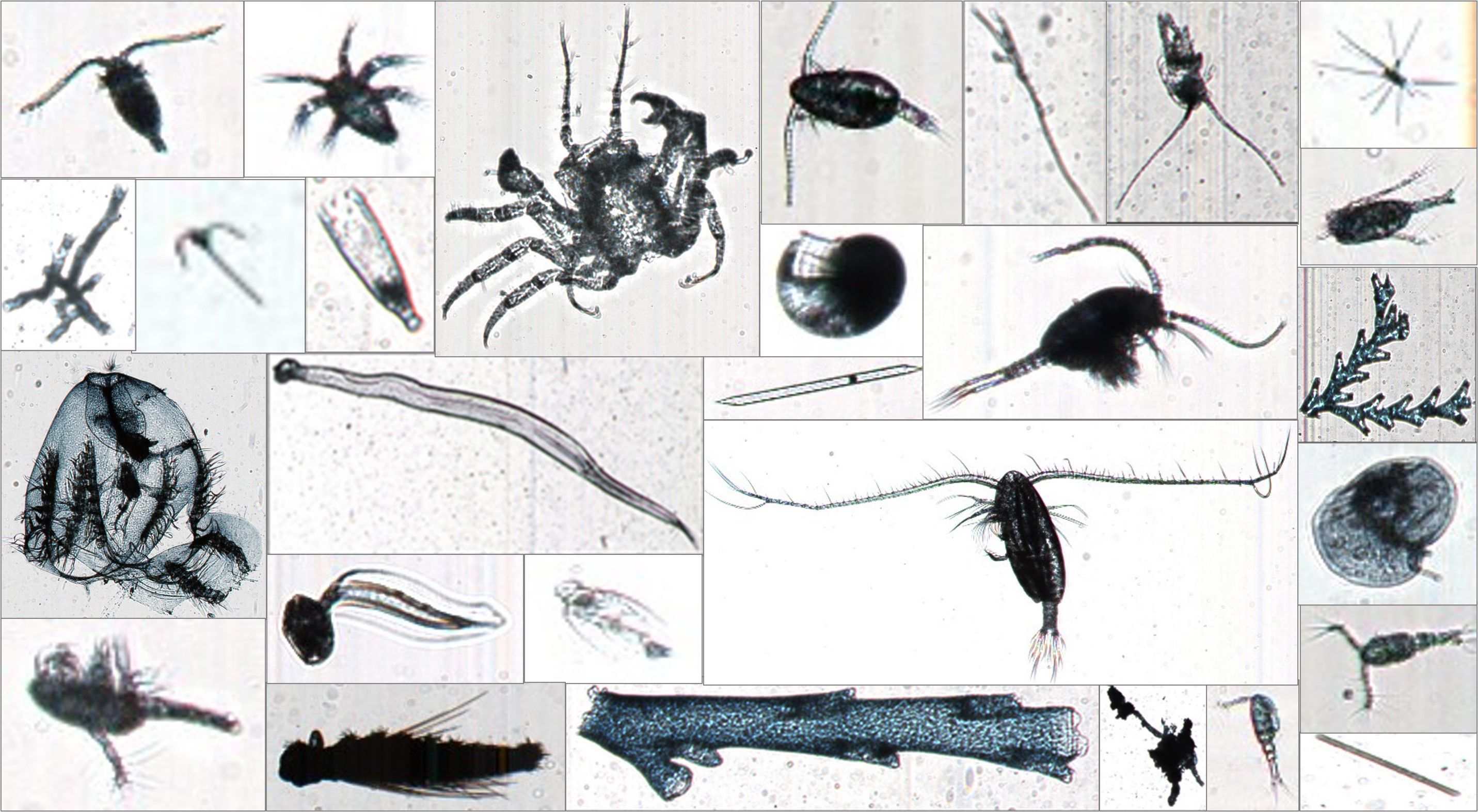
Figure 1. Example of images (not to scale) collected by the Pi-10.

2.1 System design

RAPID consists of a Plankton Imager Pi-10 instrument connected to two computers. The first computer (the “Edge AI”) is an NVIDIA Jetson AGX Orin, used for image processing and classification. Every 1 minute, the NVIDIA Jetson sends summary data (counts of Copepods, Non-Copepods and Detritus) to a terrestrial digital dashboard hosted in the cloud, via the ship’s broadband satellite communication systems. The second computer is a laptop (the “storage system”) used to store images on a solid-state drive (SSD). We use SSDs from Microsoft (Microsoft Azure Databox Disk, https://learn.microsoft.com/en-us/azure/databox/data-box-disk-overview) because they can be shipped to Microsoft post survey, who then transfer their data to cloud storage for subsequent processing in a machine learning environment. The processed data can then be stored on local servers. A high-level design schematic is shown in Figure 2.

Figure 2

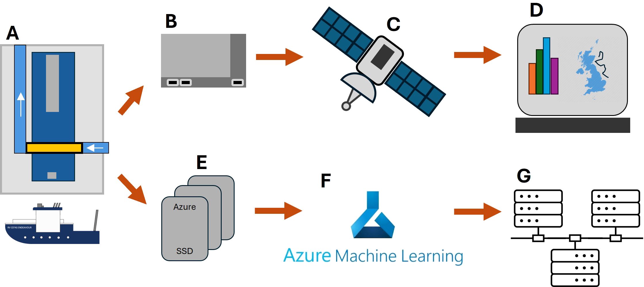
Figure 2. RAPID Plankton hardware schematic. The Pi-10, connected to the water supply aboard the RV Cefas Endeavour (A) collects images of plankton passing through a flow cell. The image stream is broadcast to an NVIDIA Jetson (B) where images are classified in real time. Summary statistics are sent via satellite (C) to a digital dashboard (D) where they can be viewed in real time. Data from the Pi-10 are also written to an Azure™ data pack (E) before being uploaded to blob storage where Azure ML is performed (F). Classified images and data are stored on local servers (G).

2.2 The classifier

In 2021, The Alan Turing Institute (London, UK) hosted a Data Study Group to look at the problem of automated plankton classification (Data Study Group, 2022). A dataset of labelled images (n = 56,991) collected with the plankton imager PI, consisting of Copepods (n = 10,275), Non-Copepods (i.e. other zooplankton, n = 6,716), and Detritus (n = 40,000) was assembled by plankton taxonomists. Copepods were selected as a group due to their prevalence within zooplankton communities, their importance as food for higher trophic levels, in particular juvenile stages of commercial fish species, and their distinctive shape. The dataset was split into training images (n = 51,309) and test images (n = 5,682). A ResNet 50 model (He et al., 2016) was implemented in Python language using TorchVision library with default number of weights for the three classes. The model was trained for 25 epochs on a 40,000:11,309 training-validation split. Training took approximately eight hours on an NVIDIA GeForce GTX 1050 Ti graphics processing unit. Accuracy results of 94-99% were obtained across all label levels when comparing the proposed ResNet architecture with baseline models (74-92% accuracy).

Deployment of this ResNet 50 model on new data collected by the PI looked promising, but accuracy and reliability diminished when the camera system was upgraded for the latest iteration of the plankton imager instrument Pi-10. This necessitated a new classifier which was developed in 2023 following the creation of a dataset of labelled images collected with the Pi-10 (n = 145377), consisting of Copepods (n = 6948), Non-Copepods (n = 1807), and Detritus (n = 136622). A ResNet 18 model was trained using transfer learning (Huh et al., 2016) and weighted cross-entropy (Ho and Wookey, 2019). Eight different versions of the ResNet model were validated on the test set. Each class’s performance was determined from calculating the parameters Precision, Recall and F1 score. Precision is the proportion of true positive predictions relative to all predicted positives. For example, precision quantifies how many of the images classified as Copepods were actually Copepods. Recall is the proportion of actual positives correctly identified. For instance, recall measures the ability of the model to correctly classify all Copepod samples as Copepods. F1 Score is the harmonic mean of precision and recall, which balances these metrics and is particularly useful for imbalanced datasets. F1 is sensitive to both false positives and false negatives, making it a comprehensive measure of model performance.

After determining the above performance parameters, we used macro-averaging to calculate the arithmetic mean for all the classes to help select the best performing model. The macro-average assigns the same weight to each class, regardless of the number of instances, which makes this a good metric in imbalanced datasets.

2.3 Edge AI

The classifier described above is run in inference mode on an NVIDIA Jetson AGX Orin running at 50W. Custom software was developed in Python to i) handle the receipt of images via User Datagram Protocol (UDP), ii) classify the images, and iii) send summary statistics to the terrestrial digital dashboard, pushing data to an Azure Service Bus queue. The queue is shared by the Python application and the dashboard working on a publish-subscribe basis with the Python application sending data as serialised JSON and the dashboard receiving that data. The queue stores the information durably, thus allowing for the dashboard to receive and process information messages in the same order in which they were sent by the Jetson custom software, but at different times and rates. Development and refining of the Edge AI software is a continuing process, with all versions recorded and shareable via GitHub on request.

2.4 Digital dashboard

Once dequeued from the Microsoft Azure Service Bus Queue, summary statistics are entered into a SQL database and then broadcast to a web application [Home page - Cefas RV Dashboard (cefastest.co.uk)] that displays summary graphs on counts and sizes of Copepods, Non-Copepods and Detritus (Figure 3). The dashboard is interactive, and the user can select to view additional graphs focusing on one class only rather than as a stacked bar chart. If the ‘streaming’ option is enabled, users can watch the map and the charts on the dashboard update in real time. The dashboard is an Asp.Net Core application written in the C# and JavaScript programming languages. The charts use the Chart.js library and the mapping functionality uses Leaflet. The real-time update capability is achieved using SignalR, a Microsoft library with a front-end and a back-end component that wraps the WebSocket functionality provided by modern web browsers.

Figure 3

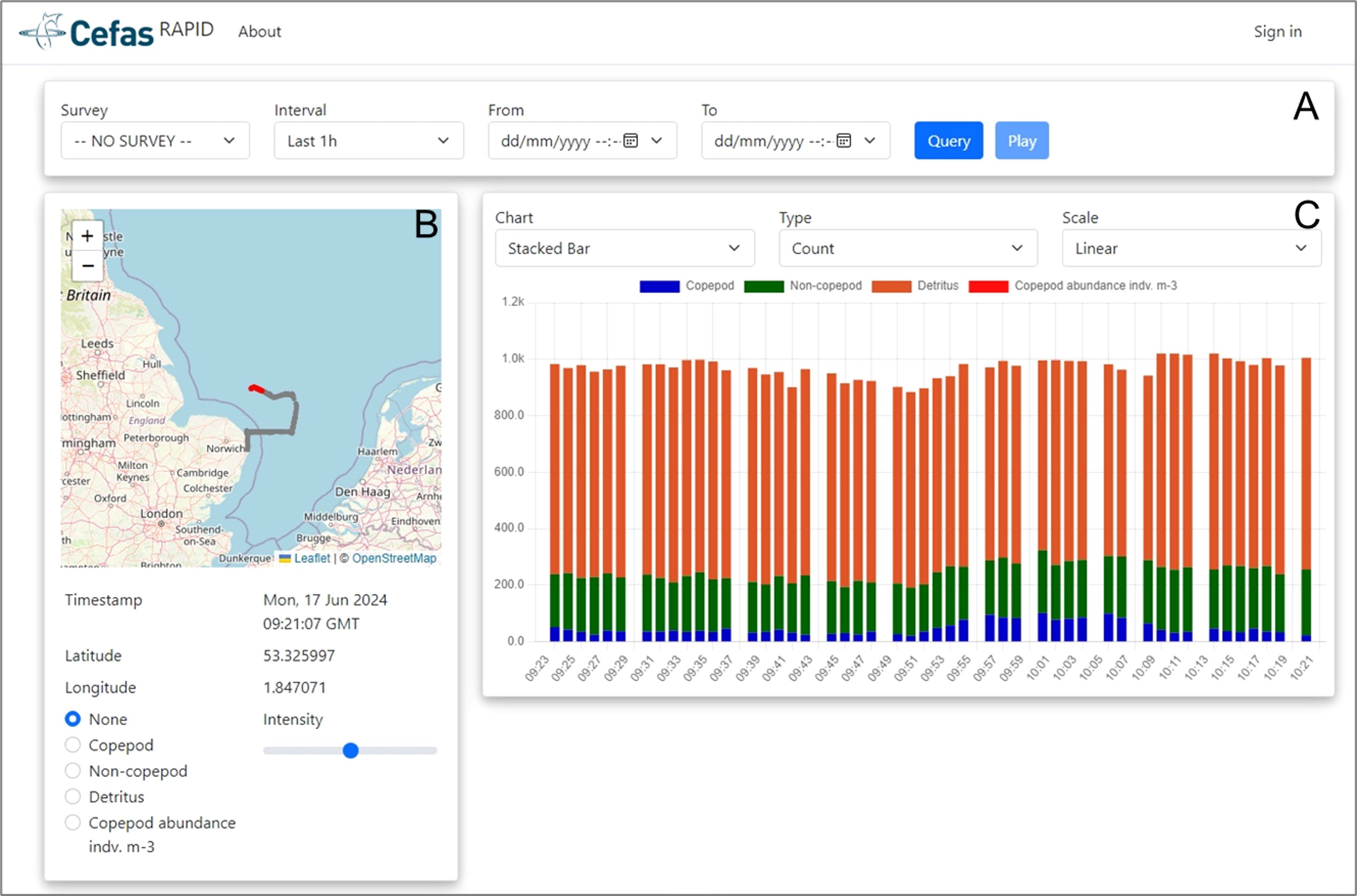
Figure 3. Screenshot of RAPID digital dashboard. (A) Menu barre for the user to select the data they wish to visualise, including time interval to group data points. (B) Current location of the RV Cefas Endeavour and recent survey tracks. The user can select the option to view counts of Copepods, Non-Copepods or Detritus on tracks. (C) The user can select what to visualise (i.e. counts or size of Copepods, Non-Copepods and Detritus) using a bar chart, line or scatter plot and onto a linear or logarithmic scale.

2.5 Storage system

While the Edge AI system shares small packets of summary statistics over the ship’s satellite data connection, raw unclassified plankton images and associated GPS information are prohibitively large to share in this way. These were instead saved locally to an azure ‘data box’ encrypted SSD, which was periodically removed and swapped out. The upload of the saved data to a data centre is handled by Microsoft and destined for an Azure blob store. This approach allowed for expandable encrypted storage with multiple backups. The blob storage can be operated on via desktop-hosted software or using scalable cloud-based computing. Both the quantity of data stored and the rate at which it can be accessed is scalable via the data storage subscription.

When handling images, the Pi-10 can be subject to internal bottlenecks from RAM, ethernet, or hard drive write speeds. In situations of high particle density in the sampled water, the Pi-10 hard drive cannot process the high number of images captured by the camera. Thus, the data collection rate becomes faster than the processing rate. When this situation arises, the instrument computer is not capable of saving all images, while simultaneously recording the number of particles that passed through the system. Images successfully captured and written to disk are called “hits”, while images captured by the camera that could not be saved to disk are called “misses”, both of which are recorded. This is akin to subsampling, with more sub-sampling required in areas or times of high particle density (Scott, personal communications).

2.6 Evaluation of real-time data pipeline and visualization

The system outlined above was deployed on the Cefas RV Endeavour, from 17^th to 23^rd May 2024. The ship progressed through the survey area, travelling from station to station where it stopped for primary sampling activities (Figure 4). The Pi-10 ran continuously during this 7-day and 5 hours period.

Figure 4

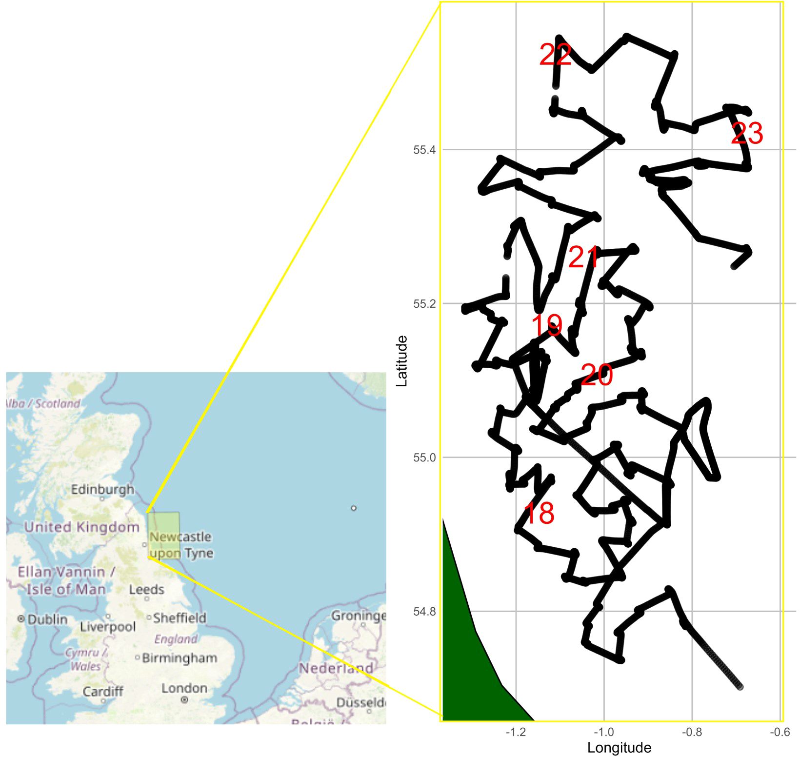
Figure 4. Survey area and vessel tracks between 17th and 23rd May 2024. Red numbers indicate the date in May 2024 at the start of a new day.

We explored the performance of the Edge AI in relation to that of the Pi-10 system, by recording (1) the number and rate of particles captured, and images saved onto disk from the instrument (i.e. “hits” and “misses”), (2) the number of images processed via the Jetson, and (3) the number of images received by the dashboard. The results were compared to identify whether there was any data loss along the pipeline, and whether any data loss would likely affect inferences drawn from the data accessible from the dashboard. All data captured by the Pi-10 were saved onto disk and sent to Microsoft for uploading onto Azure cloud storage. This dataset was processed post-survey using the same classifier as that deployed on the Edge AI Jetson, by batch classifying on a standard NC24ads computer running an A100 processor (24 cores, 220 GB RAM, 64 GB disk). Outputs from both post-survey processing and dashboard visualisation were aggregated in matching ten-minute time bins, for exploration and comparison of abundances and distribution for the 3 groups: Copepods, Non-Copepods and Detritus. This was to evaluate the performance of the Edge AI processing and real-time visualisation. A chi-squared test was performed to test whether the “observed” data used by the Edge AI corresponded with the “expected” data from post-processing, or if the two datasets were independent. This nonparametric test was chosen because our data was bi-modal, likely due to whether bubbles were present in the intake or not.

3 Results

3.1 Classifier’s performance

The classification (ResNet) model was optimised by incorporating pre-trained weights and applied grid search to adjust critical hyperparameters, such as the number of epochs and learning rate. Out of the eight versions of the ResNet model tested, the best-performing model, Model 8, consistently outperformed the other models, demonstrating superior performance across the three metrics for precision, recall, and F1 score (Figures 5A–C). This model utilises transfer learning with a ResNet-18 architecture, specifically trained on an imbalanced dataset. To mitigate class imbalance, a weighted cross-entropy loss function was applied, enhancing its ability to accurately classify underrepresented classes. The selected model achieved a macro-average F1-score of 89%. This high accuracy indicates that the model effectively differentiates between various plankton classes, such as Copepods, Non-Copepods, and Detritus, with high precision. The confusion matrix (CM) shows above 90% True Positives (TP) for all classes except the Non-Copepods class, which shows 89.57% (Figure 5D).

Figure 5

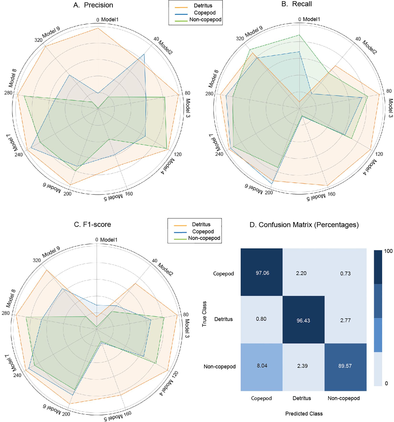
Figure 5. Radar charts illustrating the performance comparison of classification models across (A) Precision, (B) Recall, and (C) F1-Score Metrics; and (D) confusion matrix for model 8, selected as best overall performer. Each row of the confusion matrix represents an actual class example, and each column represents the state of a predicted class. The numbers on the diagonal indicate the correct predictions for each class, while the off-diagonal numbers show misclassifications between the classes.

3.2 Pi-10 instrument performance

The instrument worked continuously throughout the 7-day survey (173 hours), capturing a total of 2,997,309,347 (just under three billion) particles (Table 1). Of these, over 128 million were saved to disk and shipped to cloud storage post survey (i.e. 4.28% of the total). Particles successfully imaged and saved are called “hits”, while the remaining images could not be saved and are called “misses”. Misses are, however, still accounted for. The number of particles captured by the camera ranged from 96 to 2 x 10⁷ min^-1, including 96 to 6 x 10⁴ hits min^-1 (Figure 6). This translates to an average particle detection rate of 300,663 min^-1 and an average hit rate of 12,875 min^-1.

Table 1

Table 1. Summary of transmission performance across the real-time data pipeline from capture of particles by Pi-10 camera to visualisation of zooplankton metrics on dashboard.

Figure 6

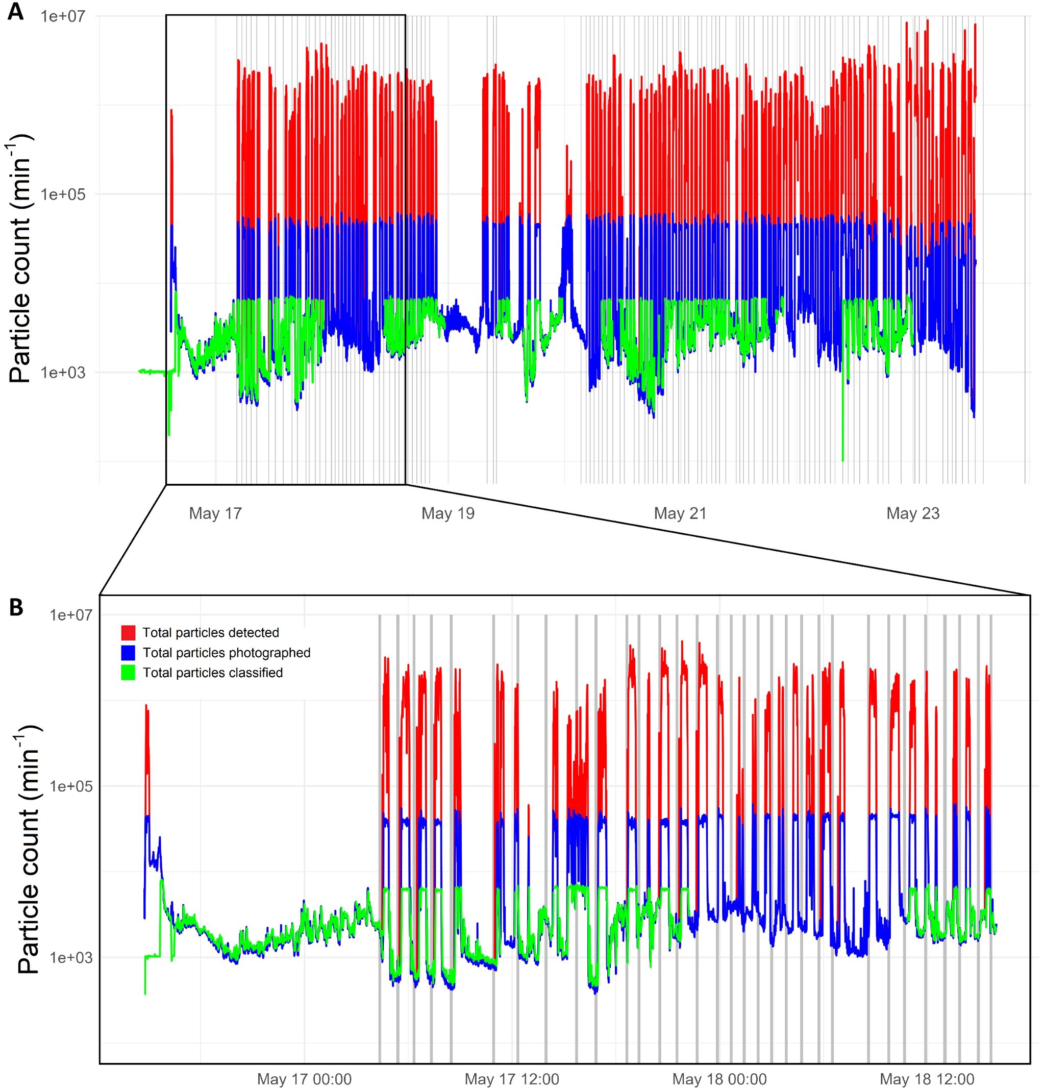
Figure 6. Number of particles detected by the camera (red line), imaged and saved to disk (blue line), and processed by the Jetson (green line), per minute over the duration of the survey (A) and a shorted extracted period between 2024-05-16 14:45:00 - 2024-05-18 16:00:00 UTC (B). The grey bands indicate when the ship was at a station, so stationary or moving very slowly. A lack of green line indicates that the jetson did not process images as it was interrupted due to the OS freezing and crashing the software.

Much higher particle and associated image capture rates occurred outside of stations (i.e. when the ship sails from one station to the next, Figure 6B). When the ship was at station, therefore stationary or moving slowly, we notice two things: firstly the numbers of particles captured, imaged and processed by the Jetson were much lower than when the ship was leaving the station to steam to the next one; secondly, the number of particles captured always shot up when the ship started travelling, to levels that are beyond the capacity of the instrument. This capacity sits around 6 x 10⁴ particles min^-1 passing through the system, beyond which particles stop being imaged (i.e. misses) (Figure 7). Essentially, there were two clear populations for the data falling at station versus in between stations, with respective mean numbers of imaged particles being 206,272 and 299,452 min^-1. A Wilcoxon rank-sum test yielded a p-value of 2 x 10^-14, indicating that this difference was almost certainly not due to chance. This supports our hypothesis that the difference was caused by movement of the ship, which anecdotally is known to cause bubbles in the Pi-10 water supply line. These bubbles were clearly visible on the resulting images.

Figure 7

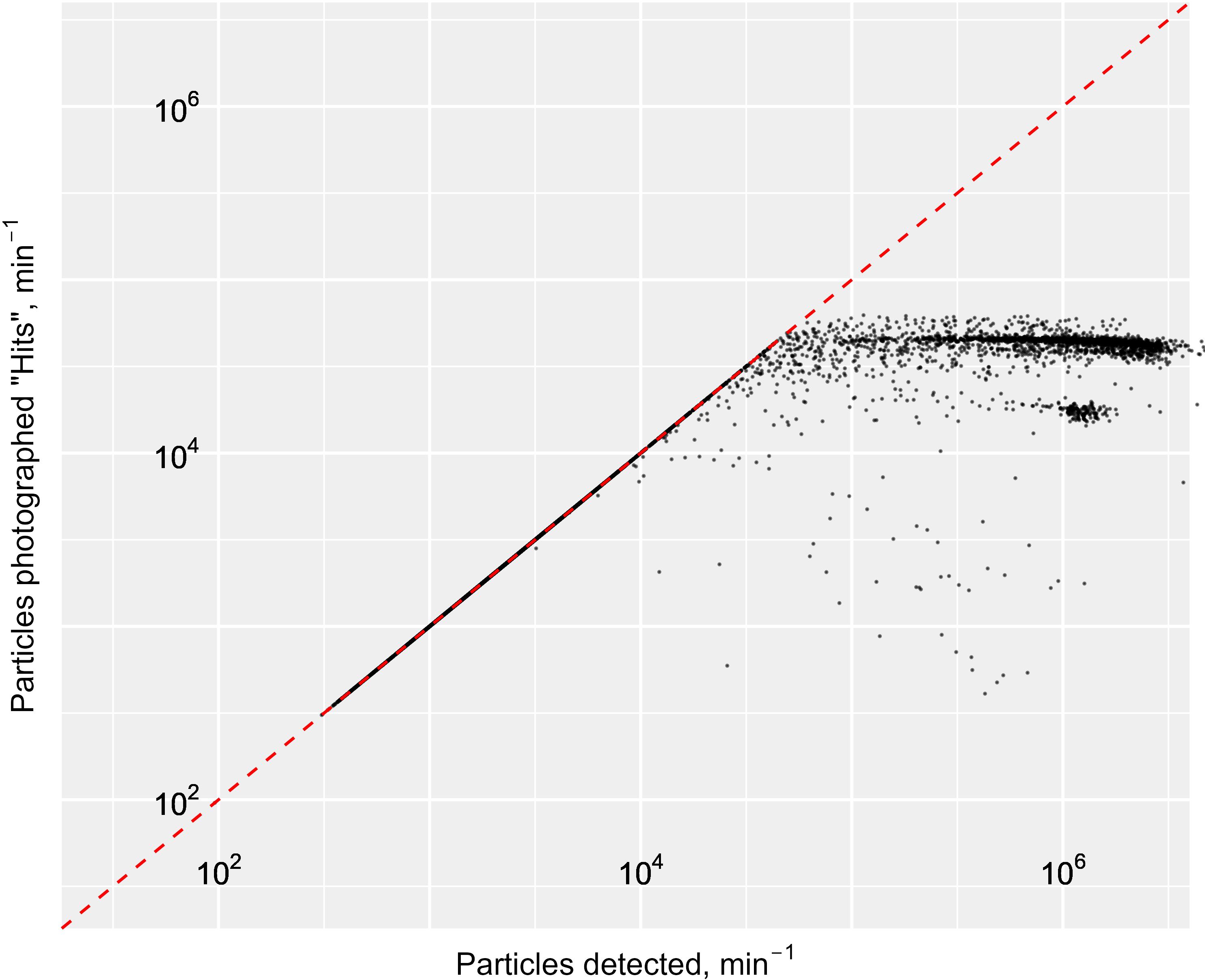
Figure 7. Log-log scatter plot of number of images successfully captured and saved (i.e. hits) vs total number of particles captured by the Pi-10 camera per minute. The dashed red line indicates the maximum capacity of the camera system with all particles detected successfully imaged and saved. As the number of particles detected increases beyond approximately 6 x 10⁴ min^-1, these stop being saved (i.e. they are misses) and points on the plot start to deviate from the red line, indicating that images are captured beyond the capacity of the camera system.

3.3 Edge AI performance

Over the 173-hour survey, 73 hours were identified as ‘downtime’. These were due to OS failure. After several hours of continuous operation, OS freezes occurred at irregular times during the survey. This was a known issue. The Python Edge AI software is in early development, running on open-source Linux OS libraries, which are themselves also subject to improvements and regular changes. For this reason, long periods can be seen in Figure 6 where no green line is present indicating the system was not running.

In the 100 operational hours the Jetson classified, measured, summarised and transmitted summary statistics for between 100 and 8,000 images min^-1, resulting in a total of 17.1 million images over the duration of the survey (i.e. 13.3% of the images transferred from the Pi-10) and an average processing rate of 2,833 images min^-1. Similarly to the Pi-10, the Jetson capacity was exceeded only when the system was flooded with bubbles (Figure 6), therefore at the start of travel in between stations. At these times, the imaged particles could not all be processed by the Jetson, demonstrating that the Jetson maximum processing capability was below that of the Pi-10. That capacity sits around 8,000 images processed min^-1 (Figure 8), beyond which images were not processed and lost from the real-time pipeline, as the Jetson software does not keep track of the number of images it receives.

Figure 8

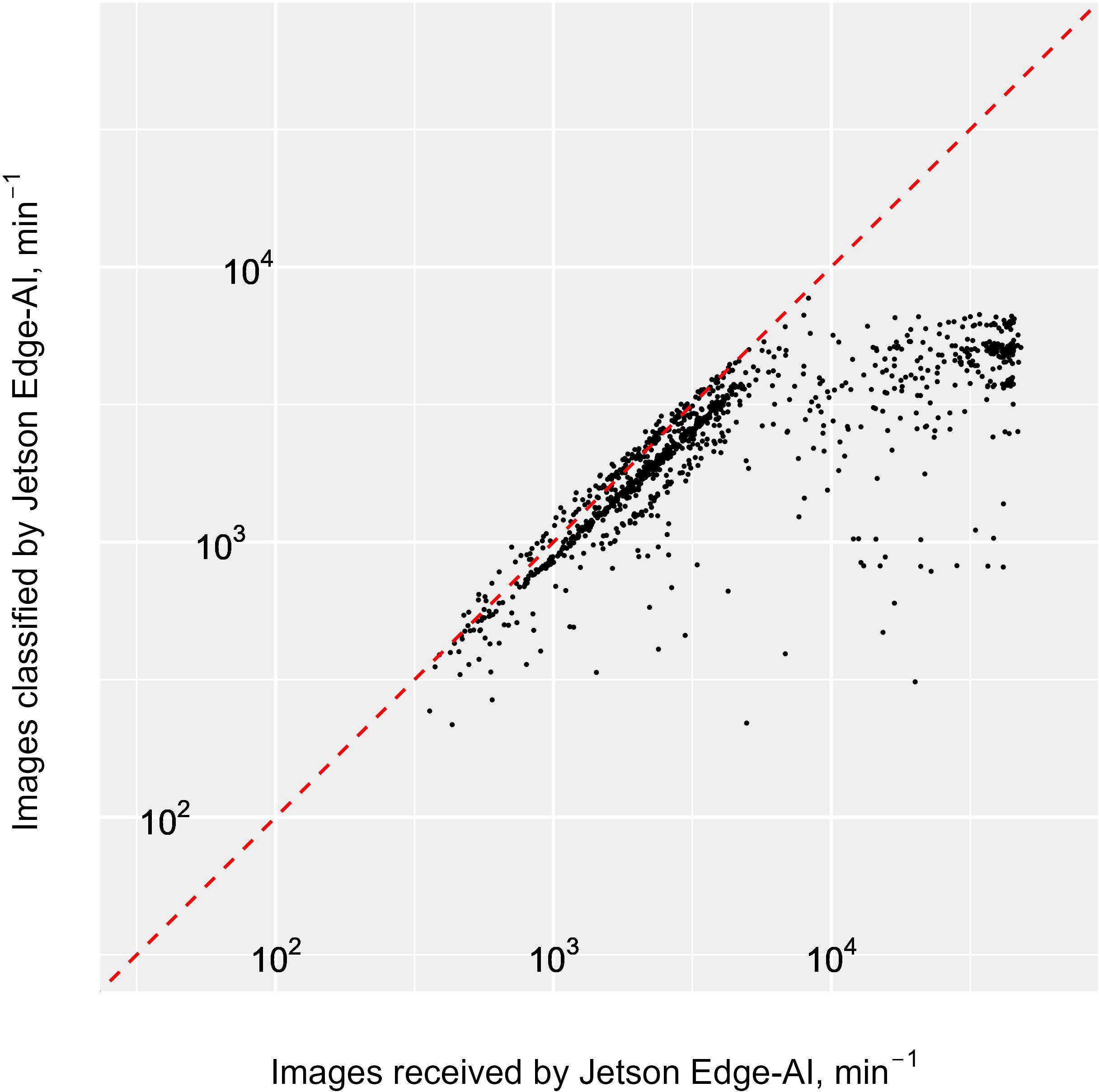
Figure 8. Log-log Scatter plot of number of images classified by the Jetson in real time vs. number of images successfully captured and saved, and sent to the Jetson by the camera (hits). Both the Pi-10 and the Jetson were set to a 60 second reporting interval, but clocks for these intervals were not synchronised across systems. Consequently, we binned data reported by the Jetson and the Pi-10 into 5-minute periods for comparison. Some degree of dyssynchrony remained and the dots on the graphs can appear marginally above the dashed red line. This line indicates that the number of images classified by the jetson is equal to the number of images received (i.e. the maximum capacity of the jetson). As the number of particles detected increases beyond approximately 8,000 min^-1, these stop being processed by the jetson and points on the plot start to deviate from the red line, indicating the maximum capacity of the jetson has been exceeded.

3.4 Transmission performance

Over the 7 days and 5 hours duration, 73 hours were identified as ‘downtime’ when the dashboard did not receive any data for over 2 minutes. This is equal to a downtime of 42% and is a reflection of all data losses due to the Jetson OS freezes and transmission losses resulting from internet connection failure. In the absence of an internet connection, the Jetson’s publishing service failed to initiate a connection to the subscribing port. This exception was not handled and consequently, the real-time system lost this data. As the system is not designed to retain failed and unsent JSON summaries, this resulted in some information loss between the Jetson to the dashboard. There were many occasions when the total number of particles transmitted to the dashboard was lower than the number of particles classified by the Jetson within a 5-minute time slot (Figure 9). This transmission loss was not dependent on the Jetson processing capacity as the size of the summary statistic packet is unrelated to the processed count but was rather a reflection of internet availability.

Figure 9

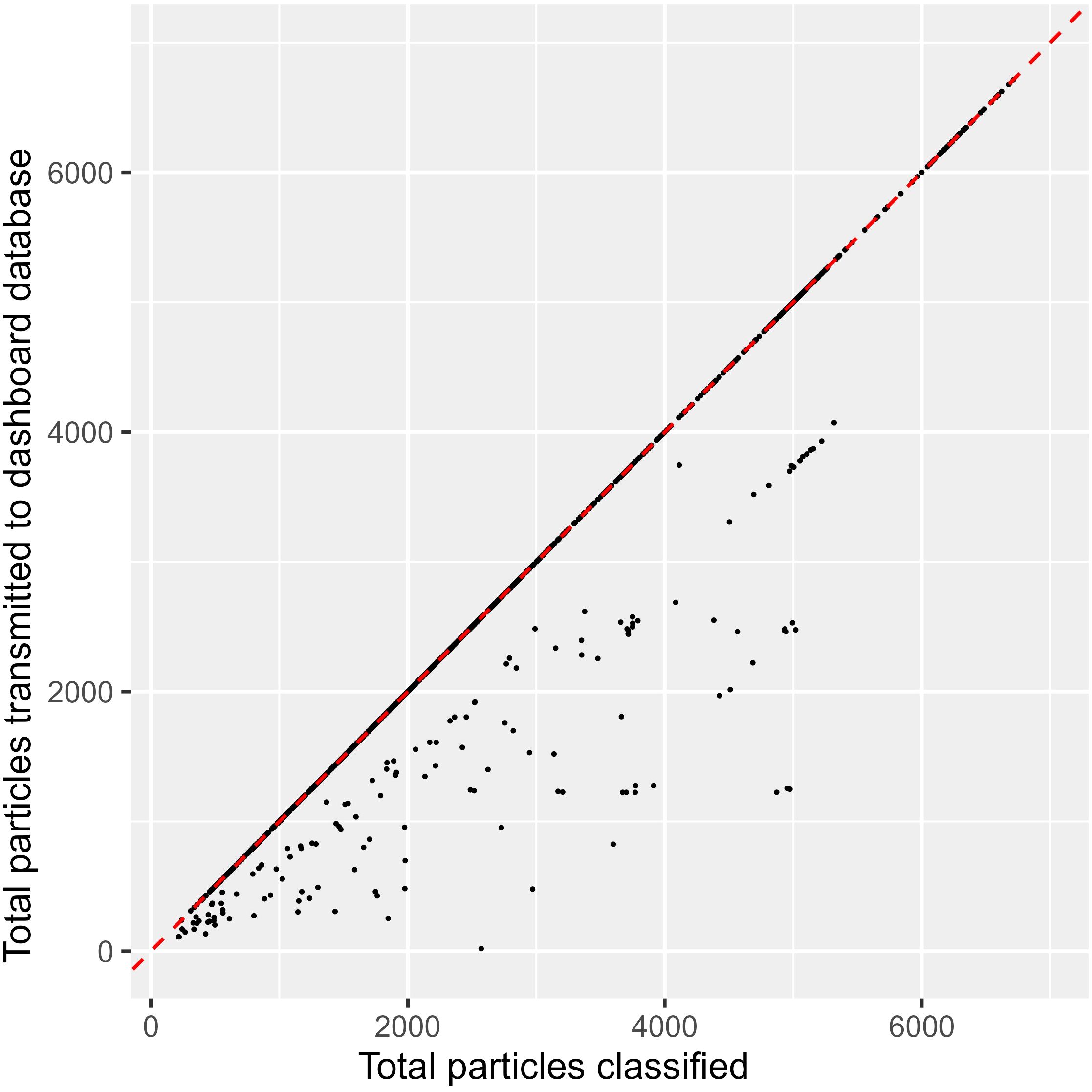
Figure 9. Scatter plot number of particles sent by the jetson to the dashboard vs number of particles classified within 5-minute bins. The red dashed line indicates that all particles classified in real-time are successfully sent to the dashboard. ‘Transmission losses’ fall on the right side of this line, where summary statistic totals within these 5-minute bins do not equal the total number of particles known to have been classified on the Jetson.

Overall, the Pi-10 captured almost 3 billion particles and successfully imaged over 128 million of them (4.28%). These images were both saved to disk for post survey processing and sent to the Jetson for real time processing using Edge AI. 17.1 million (13.25%) of the images received by the Jetson were successfully classified and the resulting information sent to the dashboard. Out of these information records, 14.8 million records (87%) were successfully received and visualised on the dashboard (Table 1). The overall output was 0.5% of particles captured by the Pi-10 were successfully imaged, processed and the resulting information sent for visualisation in real time. This suggests that the instrument capacity to image and save captured particles was the biggest limiting factor, followed by the jetson capacity to process the received images as well as its recurrent OS freezes, and finally internet availability to allow for the dashboard to receive the sent information.

3.5 Digital dashboard

Throughout the survey, the dashboard displayed a maximum value of around 8,000 particles captured min^-1 (Figure 10A), which was set by the processing capacity of the Jetson and only reached at times of likely bubbles injection through the system when the ship started travelling. There were occurrences when the dashboard didn’t display any results due to Jetson OS freezes and/or internet connection failure, as described above. Overall, the majority of particles were classified as Detritus (average 48.3%, varying from 11% to 98%), followed by Copepods (average 33.3%, varying from 0% to 70%) and Non-Copepods (18.4%, varying from 0% to 88%) (Figure 10B). The distribution of imaged particles differed when the ship was at station and started travelling to the next station (Figure 11), with Copepods being the majority class at station and Detritus the majority class outside of station, thus suggesting that bubbles were likely classified as Detritus.

Figure 10

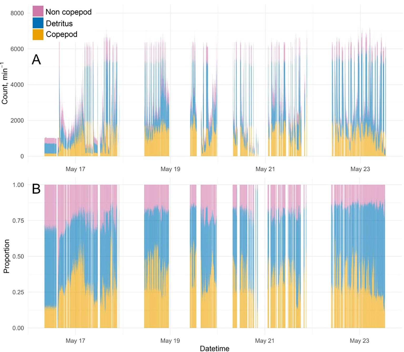
Figure 10. Summary statistics transmitted by the Jetson, received, saved to Azure SQL database and visible on the plankton dashboard [Home page - Cefas RV Dashboard (cefastest.co.uk)] (A) actual counts of Copepods, Non-Copepods and Detritus; (B) relatives counts.

Figure 11

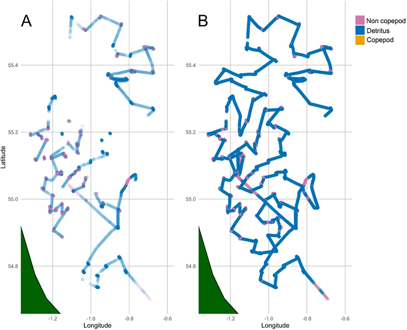
Figure 11. Dominant class along survey tracks from real-time processing via Edge AI (A) and post-processed data via cloud computing (B).

3.6 Post survey processing

Following processing of the entire saved dataset, we extracted 575 10-minute bins matching the output of the dashboard between 2024-05-16 15:00:00 - 2024-05-22 23:50:00 for comparison. These bins contained 14.5 million and 66.9 million images classified in real time and post-survey, respectively. This large difference is a result of the inability of the Jetson to process all the images saved by the Pi-10 for transfer to the real-time pipeline.

At station, the Jetson processed all images sent by the Pi-10. As a result, the output from Edge AI matched that of the dataset processed post-survey through Azure machine learning compute jobs, showing both similar dominant taxa (Figure 11) and counts (Figure 12). Outside of station, when large spikes of bubbles flooded the system (Figure 6), the resulting number of images exceeded the computing ability of the Edge AI system, and consequently, the counts from the Edge AI and post-processed results began to diverge (Figure 13). A Chi-square test confirms this with a significant difference between the counts from the two platforms (Azure and Edge AI) across the counts for Copepods, Non-Copepods, and Detritus. With a Chi-squared value of 10,659 and a p-value smaller than 2.2 x 10^-16, the result is highly significant. This means the distribution of counts for these categories differs substantially between the two platforms. Cloud computing and Edge AI are not counting the categories similarly, so a null hypothesis of no difference must be rejected. The adjusted residuals from the Chi-squared indicate where these differences lie. Post-survey processing counted significantly more Detritus (adjusted residual = 99.57) than Edge-AI processing (adjusted residual = -99.57). Additionally, post-survey processing returned significantly lower counts of Copepods and Non-Copepods (adjusted residuals = -73.13, -26.81 respectively) than Edge-AI processing (adjusted residuals = 73.13, 26.81 respectively). These significant (>1.96) residuals indicate that the discrepancies between the two platforms were not random but systematic, suggesting that post-survey processing identified more particles as Detritus in favour of the other classes. This is what we would expect as post-survey processing is able to characterise bubbles which are recorded to disk, but were overwhelming the Edge-AI system.

Figure 12

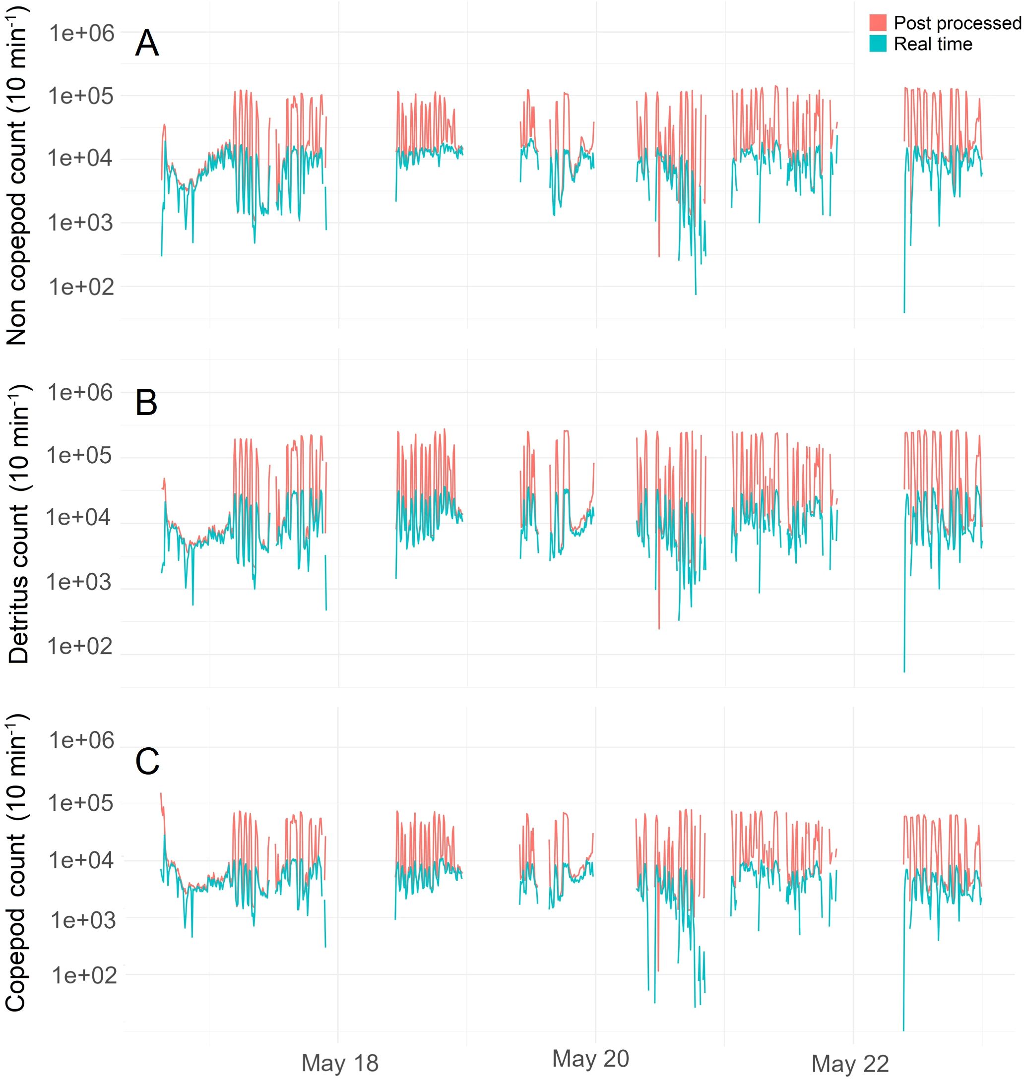
Figure 12. Summary statistics resulting from processing of images with Edge AI (green line) and cloud computing post survey (red line): counts of Non-Copepods (A), Detritus (B) and Copepods (C).

Figure 13

Figure 13. Violin and box plots for counts of Copepods, Detritus and Non-Copepods, computed on Edge AI and also via Azure cloud computing post-survey. The two subplots show the distribution of counts when the ship is on station, and travelling between stations. Violin plots indicate data density using Gaussian kernel smoothing and unbiased cross-validation to select the bandwidth of the kernel.

We note also that not only the Detritus class but also the Copepods and Non-Copepods classes show ‘spikes’ when all captured images are post-processed. Since the ResNet was not trained with a class for bubbles, when presented with a bubble it is forced to select one of the three categories. This suggests that while bubbles are most likely classified as Detritus, they are also sometimes classified in the other two classes, thereby polluting the results in all classes, but mostly those of the Detritus class.

4 Discussion

We have demonstrated a system capable of collecting and processing plankton images from a flow-through system in real time, with visualisation on a dashboard within a few minutes of processing. The overall system underwent some substantial data loss along the pipeline with 0.5% of particles captured by the Pi-10 successfully imaged, processed and sent for visualisation in real time, compared to 4.3% of particles imaged and saved to disk for post survey processing. Our results identified three areas where data loss occurred: image collection with the Pi-10, image processing and classification using Edge AI, and data transfer and visualisation.

4.1 Plankton imager

The first limitation resides within the Pi-10 capacity, with a maximum rate of saved images recorded here around 6 x 10⁴ min^-1. Over a period of 7 days, over 3 billion particles were counted, but only 128 million could be imaged and saved, or 4.3% of all particles passing through the system. There is no bias towards the type or size of particles imaged and saved by the Pi-10, as the instrument simply stops imaging as soon as it reaches its processing capacity and starts again when memory has been freed (Scott, personal communications). This is akin to subsampling. We note however that the Pi-10 worked beyond its capacity only when the ship started its travel from one station to the next. We attributed this to bubbles flooding the system, as a result of increased turbulence in the water when the ship’s propellers started rotating with increasing speed, and until the ship reached constant speed.

A potential solution is the inclusion of a “bubble recognition algorithm” to run at the imaging stage. While the number of unwanted images (i.e. bubbles) saved would decrease, it is unclear whether this would result in an increased rate of desirable images saved, due to the additional processing needed. In other words, the number of particles passing through the system would be the same and the processing time saved on not saving images of bubbles would likely be then spent on identifying them instead. Furthermore, bubbles can obscure particles; therefore, it would be preferable to physically remove them before they pass through the camera flow cell. Our suspicion is that the bubbles are caused by the propeller blades as they start rotating at increasing speed when the ship starts moving at speed, and by the dynamic positioning system of the ship causing aeration of the water in the intake. This issue could for example be resolved by changing the position of the intake to a place on the ship’s hull where the water has not yet become turbulent and mixed with air. This would, however, require amending the design of the ship. Therefore, this solution is highly impractical at best, and may produce new issues resulting from the extension of the water journey through the pipes from the intake to the instrument.

4.2 Classification on Edge AI

We have built a reliable classifier that can process images fast enough for real time output to be meaningful, and that can therefore be used routinely. However, our classifier only has three broad classes (Copepods, Non-Copepods, Detritus), so the ability to process images fast and with a level of high confidence has been achieved at the cost of taxonomic resolution.

Expanding the classifier to cover more taxonomic groups is possible, and recently, the research community has been able to access enormous plankton imagery thanks to the advent of high-resolution in situ automatic acquisition technologies (e.g. Sosik and Olson, 2007; Robinson et al., 2021). Nevertheless, acquiring unbiased annotations is time- and resource consuming, and in situ datasets are often severely imbalanced (Johnson and Khoshgoftaar, 2019), with many images available for the most common species and few images available for multiple rarer species. This problem can in part be solved by using ImageNet [ImageNet (image-net.org)], a popular image database for pre-training and transfer learning. Additionally, adjusting the loss function to effectively reduce the impact of the majority class during training, and the use of macro-averaging ensures that each class contributes equally to the overall performance assessment, making it a robust metric for evaluating the classifier’s generalisation capabilities across all classes. However, the feasibility of deploying an expanded classifier for routine real-time applications depends on various factors, notably, hardware processing capacities, computational efficiency and deployment infrastructure.

Our results show that the biggest limitation is the processing capacity of the Edge AI system (or Jetson), which was 13.3% that of the Pi-10, or around 8,000 images min^-1. An expanded classifier would require more capacity, and either a more powerful processor, operating multiple Jetsons in parallel, or accepting a lower rate of images processing and data transfer for visualisation. The requirements for high taxonomic resolutions will be dependent on the specific purpose of collecting the data and those needs should be balanced against the need to obtain reliable data fast.

In this study, the capacity of the Jetson was also exceeded only at the time of bubbles flooding the system. Results suggest that bubbles were most likely placed in the class of Detritus, but also polluting the Copepods and Non-Copepod classes, because bubbles images were not actual part of a training set. While removing bubbles from the data as soon as they are detected by the Pi-10 seems either impractical or an inefficient way of using computer resources, our results suggest that the troublesome bubbles also distorted our results. Therefore, identifying bubbles at the classification stage would be useful to separate them from the Detritus and other categories, even if this extra processing may slow down the data flow and result in some additional data loss. Since bubbles are distinctly opaque, smooth and symmetrical, multiple options exist for computational bubble detection. The first and simplest solution may be to require a minimum score before a class is accepted.

4.3 Data transfer and connectivity

A major challenge of transferring data from offshore locations is having reliable internet. While we had some transmission losses resulting from internet connectivity failure, this was relatively small (13%) compared to the interruptions in data transfer from the Jetson. The success rate of 87% is reflective of the ability to report back “within the minute” given the current internet infrastructure installed on the ship. When the internet becomes unavailable, the Jetson is unable to retain unsent summary data packets which then disappear from the pipeline. Internet connectivity is beyond our control but there are mitigations that can be put into place, such as defining an outgoing reporting data queue so that summary statistics persist beyond the 5-minute reporting period. This solution has been successfully implemented in a subsequent survey, meaning unsuccessful transmissions are now backfilled after the connection is reestablished. This of course means that, when internet connectivity is lost, visualisation is not done in real time anymore, but that is only a temporary feature and certainly better than no visualisation at all.

The Jetson Operating System crashes posed a greater issue. Those interruptions were related to the Jetson computer becoming unresponsive rather than connectivity. Following this first deployment and the results presented in this manuscript, two relevant changes have been implemented: Firstly, a limit has been imposed on the maximum length of the image queue held in memory on the Jetson computer. Thus, the Jetson now operates similarly to the Pi-10, pausing saving images when the particle capture rate exceeds its capacity. Secondly, the edge AI command line tool includes an optional command line argument for –subsampling_rate. This parameter can be carefully adjusted to match the maximum throughput of the imager to prevent the system from overwriting the ring buffer (images in memory). Following those implementations, the Jetson has stopped freezing. This is an improvement, however developing a dynamic subsampling rate would be preferable. A dynamic subsampling rate that is sensitive to the ring buffer state could theoretically throttle throughput based on how full the buffer is, ensuring the system benefits from both fair 1-in-n subsampling while making the fullest use of the available computing power for inference.

4.4 Future improvements to mitigate for bubble inference and data loss

Our system transmits images for both retention and real-time classification, with the real-time classifier capable of processing a fraction (i.e. 13.2%) of the number of photographs that can be taken. Following this first study, we have successfully implemented some software changes, as described above, to address issues with the Jetson OS freezes and loss of internet connectivity.

We note however that data loss only occurred at the time of bubbles flooding the system, sending both the plankton imager and Edge AI over their processing capacity. Bubbles are inevitable within a water flow and affected this system at two stages: 1) when their numbers created bottlenecks within the data pipeline; and 2) they polluted all classes, thereby distorting the final counts within the processed classes. Consequently, our real time visualisation produced satisfactory results, similar to those produced post-survey on the entire dataset, only when the ship was at station, or sailing at regular speed; That is, when there is no surge of bubbles and when the number of images received remains within its capacity of 8,000 images min^-1.

While the processing power on the Edge AI system can be scaled up to match that of the Pi-10, the plankton imager was itself overwhelmed by bubbles when the ship started sailing, resulting in its inability to image over 95% of passing particles over the duration of the survey. In previous deployments on the plankton imager (Pitois et al., 2018, Pitois et al., 2021; Scott et al., 2021), data collection occurred at stations only, and thus, bubbles didn’t create any issues. Scott et al. (2023) were the first to use the instrument to record data continuously, but bubbles, whilst present at time, were not particularly noticeable within the data. The reasons for this discrepancy are unclear but likely related to the vessel speed which can vary depending on survey requirements. It is therefore our first encounter with the issue of troublesome bubbles creating problematic incursions.

As the Pi-10 records hits and misses, it is possible to apply a scaling factor later at the processing stage. But, unlike the Pi-10, the Jetson did not record the number of images it didn’t process, and therefore the data visible on the dashboard could not be scaled up to take into account any subsampling. This flaw has since been addressed by implementing the software changes described above. As the Jetson can now record the number of hits and misses within each data packet it sends to the dashboard, the total amount of subsampling can be calculated and the published information scaled up accordingly. While images themselves can vary in sizes and require more or less time to be processed, all resulting summary statistics are sent to the service bus queue in the form of information messages, all of the same size. These are subsequently dequeued and received by the dashboard in a sequence of the same order in which they were sent, but at different times. There is unlikely to be a bias created during this sequential process within images that cannot be processed by the Jetson at times of over-capacity. We can therefore consider this step also akin to subsampling, occurring when the Jetson operates beyond its processing capacity, and making the application of a scaling factor based on hits and misses is appropriate.

In theory, the processing power installed on the Pi-10 can also be scaled up to cater for bubble surges, and matched by that of the Edge AI, but this is conditional on substantial financial investments. Inevitably, such costs will decrease in the future. In the short term, to address data loss from Jetson and internet connectivity failures, we have already implemented changes and improvements as described above. Potential solutions to deal with bubble surges were discussed earlier and we suggest that training our classifier to include a bubble class is the way forward, to prevent bubbles polluting all other classes. These important steps can transform the dashboard from a qualitative real-time visualisation tool to one that works mostly uninterrupted and produces reliable quantitative results that can be used for real-time applications.

4.5 Limitations and strengths

Even if we implement the above suggested improvements, including a class specific for bubbles embedded within the existing algorithm, bubbles will still remain a problem for overlapping particles when present in high densities. A physical solution will need to be found at some point in the future, so as to remove them from appearing in the water flow altogether. While it is currently impossible to quantify the amount of misclassification induced by bubbles and their overlapping particles, due to the sheer quantity of images, separating bubbles from the rest of the data will be easy to implement, and should allow for real or near real-time visualisation of crude plankton groups abundances and biomass continuously throughout a survey. For more detailed classification and analysis post-survey, we recommend dismissing bins of data collected when the capacity of the Pi-10 was exceeded as these most likely relate to bubbles flooding the system. Such bins are easily identified from the number of returned misses, as on Figure 6. While this would leave gaps within the continuous data, the resolution obtained should still be satisfactory for the great majority of monitoring needs.

Even with noted improvements, our method does not currently provide the ability of monitoring species biodiversity and associated changes in real time, but it is always possible to deploy an expanded classifier at a later date on the full dataset uploaded onto cloud storage, while making the most of the real-time information provided: densities for broad taxonomic Copepods and Non-Copepods groups, their size distribution and biomass. There are three immediate applications for which our method is appropriate:

Firstly, the monitoring of trends and events at fine scales [e.g. plankton patchiness, Robinson et al. (2021)], thus making the most of the continuous data collection (Scott et al., 2023); Secondly, helping select sampling parameters and intensity at location depending on changes noted, the dashboard being the first point where changes are noted as they are happening. This is the concept of adaptive sampling, where data collection can be adapted to target parts of the ecosystem at certain time and space according to changes noted in real-time. For example, a surge in the abundance of Copepods and/or their size distribution could indicate changes in the conditions of prey for commercial fish (Pitois et al., 2021) and for which further data collection (fish and others) might be required to understand what is happening. Thirdly, to inform the selection of data to be further processed via cloud computing post survey. This last point is connected to the previous one: when changes are happening, it may be decided to fully process the images to understand any potential cause and process behind those changes. For example, running an expanded classifier on the cloud computing platform on a selected relevant subset of the entire dataset. Equally, if no change is noted at all, there may be little interest or need for further processing post-survey in the short term at least.

A key advantage of the use of our Edge AI system is its relatively low cost and ease of use: the Jetson is compact, requires low financial investment and is easy to deploy. There is also no financial cost associated with image processing, as is the case when operating in a cloud computing environment. In this particular study, processing our entire datasets of 128 million images using Azure cloud computing took 5 days on a $4/hr compute instance, equivalent to a total of ~$500. While this appears relatively small, and good value for money, it would likely not be regarded as sustainable as a continuous use or use as default for all surveys. That being said, it is important to archive all images collected. As technologies improve and become more affordable, it will be possible to process or reprocess those datasets using the latest data analytics tools.

5 Conclusion

We have demonstrated a system capable of collecting and processing plankton images from a flow-through system in real time, with online visualisation within a few minutes of processing.

Expanding the resolution of the classifier in real-time to include more detailed taxonomic groups could improve its value for biodiversity studies. This would require addressing issues such as the availability of high-quality labelled data, imbalanced class distributions, and the increased computational demands of a more complex model. Additionally, incorporating methods to handle uncertainties in predictions and adding a dedicated class for bubbles could help mitigate noise and further enhance accuracy in real-time applications. While applications of the systems are currently limited to non-biodiversity studies, gradual improvement of classifier models seems both unavoidable and inevitable given the rapid pace of improvement in AI tools. It is anticipated that more performant computer processors will be soon available that can cater for an expanded classifier to be deployed as part of our Edge AI pipeline. The Plankton Imager has been used for several years and its value for application to ecological studies has already been evidenced (Pitois et al., 2018, Pitois et al., 2021; Scott et al., 2021, Scott et al., 2023). The use of imaging and AI tools is still in its infancy, but early results suggest that technological advances in this field have the potential to revolutionise how we monitor our seas (Giering et al., 2022). Further industrial and scientific applications of this instrument are open-ended. It is only by continuing to collect and better classify image data from this new instrument that we will uncover the insights it offers, especially at the near-metre resolution.

Data availability statement

The raw data supporting the conclusions of this article will be made available by the authors upon request, without undue reservation.

Ethics statement

The manuscript presents research on animals that do not require ethical approval for their study.

Author contributions

SP: Conceptualization, Funding acquisition, Investigation, Methodology, Project administration, Resources, Supervision, Writing – original draft, Writing – review & editing. RB: Conceptualization, Funding acquisition, Investigation, Software, Writing – review & editing. HC: Data curation, Investigation, Writing – review & editing. NE: Formal analysis, Investigation, Methodology, Software, Writing – original draft, Writing – review & editing. SG: Conceptualization, Writing – review & editing. MM: Software, Writing – review & editing. EP: Software, Visualization, Writing – original draft. JR: Data curation, Formal analysis, Investigation, Methodology, Validation, Visualization, Writing – original draft, Writing – review & editing. JS: Data curation, Investigation, Visualization, Writing – review & editing.

Funding

The author(s) declare that financial support was received for the research, authorship, and/or publication of this article. Scientific cruises were funded as part of the monitoring programme at the Centre for Environment Fisheries and Aquaculture Science, part of the Department for Environment, Food and Rural Affairs. The work was supported by the Alan Turing Institute AI for Environment and Sustainability Programme, and the Cefas Seedcorn programme (DP4000).

Acknowledgments

We would like to thank the hosts, researchers and participants of the 2021 Alan Turing Institute Data Study Group for their initial work on plankton classification using deep learning. Our thanks also go to the officers, crew and scientists onboard RV Cefas Endeavour for their assistance in collecting scientific data.

Conflict of interest

The authors declare that the research was conducted in the absence of any commercial or financial relationships that could be construed as a potential conflict of interest.

Generative AI statement

The author(s) declare that no Generative AI was used in the creation of this manuscript.

Publisher’s note

All claims expressed in this article are solely those of the authors and do not necessarily represent those of their affiliated organizations, or those of the publisher, the editors and the reviewers. Any product that may be evaluated in this article, or claim that may be made by its manufacturer, is not guaranteed or endorsed by the publisher.

References

Benfield M. C., Grosjean P., Culverhouse P., Irigoien X., Sieracki M. E., Lopez-Urrutia A., et al. (2007). RAPID: research on automated plankton identification. Oceanography 20, 172–187. doi: 10.5670/oceanog.2007.63

Crossref Full Text | Google Scholar

Borja A., Berg T., Gundersen H., Gjørwad Hagen A., Hancke K., Korpinen S., et al. (2024). Innovative and practical tools for monitoring and assessing biodiversity status and impacts of multiple human pressures in marine systems. Environ. Monit. Assess. 196, 694. doi: 10.1007/s10661-024-12861-2

PubMed Abstract | Crossref Full Text | Google Scholar

Danovaro R., Carugati L., Berzano M., Cahill A. E., Carvalho S., Chenuil A., et al. (2016). Implementing and innovating marine monitoring approaches for assessing marine environmental status. Front. Mar. Sci. 3. doi: 10.3389/fmars.2016.00213

Crossref Full Text | Google Scholar

Data Study Group (2022). Data Study Group Final Report: Centre for Environment, Fisheries and Aquaculture Science, Plankton image classification (Alan Turing Institute). doi: 10.5281/zenodo.6799166

Crossref Full Text | Google Scholar

Davis C. S., Gallager S. M., Berman M. S., Haury L. R., Strickler J. R. (1992). The video plankton recorder (VPR): design and initial results. Arch. Hydrobiol. Beih 36, 67–81.

Google Scholar

Dierssen H. M., Randolph K. (2013). “Remote sensing of ocean color,” in Earth system Monitoring: Selected Entries from the Encyclopedia of Sustainability Science and Technology. Ed. Orcutt J. (New Yok, NY: Springer), 439–472. doi: 10.1007/978-1-4614-5684-1_18

Crossref Full Text | Google Scholar

Edwards M., Richardson A. J. (2004). Impact of climate change on marine pelagic phenology and trophic mismatch. Nature 430, 881–884. doi: 10.1038/nature02808

PubMed Abstract | Crossref Full Text | Google Scholar

Field C. B., Behrenfeld M. J., Randerson J. T., Falkowski P. (1998). Primary production of the biosphere: integrating terrestrial and oceanic components. science 281, 237–240. doi: 10.1126/science.281.5374.237

PubMed Abstract | Crossref Full Text | Google Scholar

Giering S. L., Culverhouse P. F., Johns D. G., McQuatters-Gollop A., Pitois S. G. (2022). Are plankton nets a thing of the past? An assessment of in situ imaging of zooplankton for large-scale ecosystem assessment and policy decision-making. Front. Mar. Sci. 9. doi: 10.3389/fmars.2022.986206

Crossref Full Text | Google Scholar

Gorokhova E., Lehtiniemi M., Postel L., Rubene G., Amid C., Lesutiene J., et al. (2016). Indicator properties of Baltic zooplankton for classification of environmental status within marine strategy framework directive. PLoS One 11, e0158326. doi: 10.1371/journal.pone.0158326

PubMed Abstract | Crossref Full Text | Google Scholar

Gorsky G., Ohman M. D., Picheral M., Gasparini S., Stemmann L., Romagnan J. B., et al. (2010). Digital zooplankton image analysis using the ZooScan integrated system. J. Plankton Res. 32, 285–303. doi: 10.1093/plankt/fbp124

Crossref Full Text | Google Scholar

Grosjean P., Picheral M., Warembourg C., Gorsky G. (2004). Enumeration, measurement, and identification of net zooplankton samples using the ZOOSCAN digital imaging system. ICES J. Mar. Sci. 61, 518–525. doi: 10.1016/j.icesjms.2004.03.012

Crossref Full Text | Google Scholar

Guo B., Nyman L., Nayak A. R., Milmore D., McFarland M., Twardowski M. S., et al. (2021). Automated plankton classification from holographic imagery with deep convolutional neural networks. Limnol. Oceanogr.-Meth. 19, 21–36. doi: 10.1002/lom3.10402

Crossref Full Text | Google Scholar

He K., Zhang X., Ren S., Sun J. (2016). “Deep residual learning for image recognition,” in Proceedings of the IEEE conference on computer vision and pattern recognition (CVPR). Las Vegas, NV, USA 770–778. doi: 10.1109/CVPR.2016.90

Crossref Full Text | Google Scholar

Ho Y., Wookey S. (2019). The real-world-weight cross-entropy loss function: Modeling the costs of mislabeling. IEEE Access 8, 4806–4813. doi: 10.1109/ACCESS.2019.2962617

Crossref Full Text | Google Scholar

Huh M., Agrawal P., Efros A. A. (2016). What makes ImageNet good for transfer learning? arXiv preprint arXiv:1608.08614. doi: 10.48550/arXiv.1608.08614

Crossref Full Text | Google Scholar

Jeffries H. P., Berman M. S., Poularikas A. D., Katsinis C., Melas I., Sherman K., et al. (1984). Automated sizing, counting and identification of zooplankton by pattern recognition. Mar. Biol. 78, 329–334. doi: 10.1007/BF00393019

Crossref Full Text | Google Scholar

Johnson J. M., Khoshgoftaar T. M. (2019). Survey on deep learning with class imbalance. J. big Data 6, 1–54. doi: 10.1186/s40537-019-0192-5

Crossref Full Text | Google Scholar

Kim J. H., Shin J. K., Lee H., Lee D. H., Kang J. H., Cho K. H., et al. (2021). Improving the performance of machine learning models for early warning of harmful algal blooms using an adaptive synthetic sampling method. Water Res. 207, 117821. doi: 10.1016/j.watres.2021.117821

PubMed Abstract | Crossref Full Text | Google Scholar

Kraft K., Velhonoja O., Eerola T., Suikkanen S., Tamminen T., Haraguchi L., et al. (2022). Towards operational phytoplankton recognition with automated high-throughput imaging, near-real-time data processing, and convolutional neural networks. Front. Mar. Sci. 9. doi: 10.3389/fmars.2022.867695

Crossref Full Text | Google Scholar

Lauria V., Attrill M. J., Brown A., Edwards M., Votier S. C. (2013). Regional variation in the impact of climate change: evidence that bottom-up regulation from plankton to seabirds is weak in parts of the Northeast Atlantic. Mar. Ecol. Prog. Ser. 488, 11–22. doi: 10.3354/meps10401

Crossref Full Text | Google Scholar

Le Bourg B., Cornet-Barthaux V., Pagano M., Blanchot J. (2015). FlowCAM as a tool for studying small (80–1000 mm) metazooplankton communities. J. Plankton Res. 37, 666–670. doi: 10.1093/plankt/fbv025

Crossref Full Text | Google Scholar

LeCun Y., Bengio Y., Hinton G. (2015). Deep learning. Nature 521, 436–444. doi: 10.1038/nature14539

PubMed Abstract | Crossref Full Text | Google Scholar

Lombard F., Boss E., Waite A. M., Uitz J., Stemmann L., Sosik H. M., et al. (2019). Globally consistent quantitative observations of planktonic ecosystems. Front. Mar. Sci. 6. doi: 10.3389/fmars.2019.00196

Crossref Full Text | Google Scholar

Masoudi M., Giering S. L., Eftekhari N., Massot-Campos M., Irisson J. O., Thornton B. (2024). Optimizing plankton image classification with metadata-enhanced representation learning. IEEE J. Sel. Top. Appl. Earth Obs. Remote Sens. 17, 17117–17133. doi: 10.1109/JSTARS.2024.3424498

Crossref Full Text | Google Scholar

Mcilwaine B., Casado M. R. (2021). JellyNet: The convolutional neural network jellyfish bloom detector. Int. J. Appl. Earth Obs. Geoinf. 97, 102279. doi: 10.1016/j.jag.2020.102279

Crossref Full Text | Google Scholar

Mitra A., Castellani C., Gentleman W. C., Jónasdóttir S. H., Flynn K. J., Bode A., et al. (2014). Bridging the gap between marine biogeochemical and fisheries sciences; configuring the zooplankton link. Progr. Oceanogr. 129, .176–.199. doi: 10.1016/j.pocean.2014.04.025

Crossref Full Text | Google Scholar

Picheral M., Catalano C., Brousseau D., Claustre H., Coppola L., Leymarie E., et al. (2022). The Underwater Vision Profiler 6: an imaging sensor of particle size spectra and plankton, for autonomous and cabled platforms. Limnol. Oceanogr.-Meth. 20, 115–129. doi: 10.1002/lom3.10475

PubMed Abstract | Crossref Full Text | Google Scholar

Picheral M., Guidi L., Stemmann L., Karl D. M., Iddaoud G., Gorsky G. (2010). The Underwater Vision Profiler 5: An advanced instrument for high spatial resolution studies of particle size spectra and zooplankton. Limnol. Oceanogr.-Meth. 8, 462–473. doi: 10.4319/lom.2010.8.462

Crossref Full Text | Google Scholar

Pitois S. G., Graves C. A., Close H., Lynam C., Scott J., Tilbury J., et al. (2021). A first approach to build and test the Copepod Mean Size and Total Abundance (CMSTA) ecological indicator using in-situ size measurements from the Plankton Imager (PI). Ecol. Indic, 123. doi: 10.1016/j.ecolind.2020.107307

Crossref Full Text | Google Scholar

Pitois S. G., Lynam C. P., Jansen T., Halliday N., Edwards M. (2012). Bottom-up effects of climate on fish populations: data from the Continuous Plankton Recorder. Mar. Ecol. Progr. Ser. 456, 169–186. doi: 10.3354/meps09710

Crossref Full Text | Google Scholar

Pitois S. G., Tilbury J., Close H., Barnett S., Culverhouse P. F. (2018). Comparison of a cost-effective integrated plankton sampling and imaging instrument with traditional systems for mesozooplankton sampling in the celtic sea. Front. Mar. Sci. 5. doi: 10.3389/fmars.2018.00005

Crossref Full Text | Google Scholar

Pitois S., Yebra L. (2022). Contribution of marine zooplankton time series to the United Nations Decade of Ocean Science for Sustainable Development. ICES J. Mar. Sci. 79, 722–726. doi: 10.1093/icesjms/fsac048

Crossref Full Text | Google Scholar

Ratnarajah L., Abu-Alhaija R., Atkinson A., Batten S., Bax N. J., Bernard K. S., et al. (2023). Monitoring and modelling marine zooplankton in a changing climate. Nat. Commun. 14, 564. doi: 10.1038/s41467-023-36241-5

PubMed Abstract | Crossref Full Text | Google Scholar

Robinson K. L., Sponaugle S., Luo J. Y., Gleiber M. R., Cowen R. K. (2021). Big or small, patchy all: Resolution of marine plankton patch structure at micro-to submesoscales for 36 taxa. Sci. Adv. 7, eabk2904. doi: 10.1126/sciadv.abk2904

PubMed Abstract | Crossref Full Text | Google Scholar

Rolke M., Lenz L. (1984). Size structure analysis of zooplankton samples by means of an automated image analyzing system. J. Plankton Res. 6, 637–645. doi: 10.1093/plankt/6.4.637

Crossref Full Text | Google Scholar

Schmid M. S., Daprano D., Damle M. M., Sullivan C. M., Sponaugle S., Cousin C., et al. (2023). Edge computing at sea: high-throughput classification of in-situ plankton imagery for adaptive sampling. Front. Mar. Sci. 10. doi: 10.3389/fmars.2023.1187771

Crossref Full Text | Google Scholar

Scott J., Pitois S., Close H., Almeida N., Culverhouse P., Tilbury J., et al. (2021). In situ automated imaging, using the Plankton Imager, captures temporal variations in mesozooplankton using the Celtic Sea as a case study. J. Plankton Res. 43, 300–313. doi: 10.1093/plankt/fbab018

Crossref Full Text | Google Scholar

Scott J., Pitois S., Creach V., Malin G., Culverhouse P., Tilbury J. (2023). Resolution changes relationships: Optimizing sampling design using small scale zooplankton data. Progr. Oceanogr 210, 102946. doi: 10.1016/j.pocean.2022.102946

Crossref Full Text | Google Scholar

Serranito B., Aubert A., Stemmann L., Rossi N., Jamet J.-L. (2016). Proposition of indicators of anthropogenic pressure in the Bay of Toulon (Mediterranean Sea) based on zooplankton time-series. Cont. Shelf Res. 121, 3–12. doi: 10.1016/j.csr.2016.01.016

Crossref Full Text | Google Scholar

Sosik H. M., Olson R. J. (2007). Automated taxonomic classification of phytoplankton sampled with imaging-in-flow cytometry. Limnol. Oceanogr.-Meth. 5, 204–216. doi: 10.4319/lom.2007.5.204

Crossref Full Text | Google Scholar

Strömberg K. H. P., Smyth T. J., Allen I. J., Pitois S., O'Brien T. D. (2009). Estimation of global zooplankton biomass from satellite ocean colour. J. Mar. Syst. 78, 18–27. doi: 10.1016/j.jmarsys.2009.02.004

Crossref Full Text | Google Scholar

Tang X., Stewart W. K., Huang H., Gallager S. M., Davis C. S., Vincent L., et al. (1998). Automatic plankton image recognition. Artif. Intell. Rev. 12, 177–199. doi: 10.1023/A:1006517211724

Crossref Full Text | Google Scholar

Wiebe P. H., Benfield M. C. (2003). From the Hensen net toward four-dimensional biological oceanography. Prog. Oceanogr. 56, 7–136. doi: 10.1016/S0079-6611(02)00140-4

Crossref Full Text | Google Scholar