Turbulence and mixing variability in a microtidal estuary subject to mixed semidiurnal tidal cycles

Reynolds stresses and Turbulent Kinetic Energy (TKE) are instrumental in quantifying the turbulent dynamics that govern mixing and momentum transport in estuaries, factors crucial for understanding and managing estuarine circulation, water quality, and sediment transport. Employing Acoustic Doppler Current profilers, this study investigated hydrodynamics and turbulence in the Brisbane River, Australia. Measurements were conducted at two locations, covering the mouth and middle reach of the estuary. Of particular interest were flow reversals during flood flows, adding complexity to the turbulent dynamics. Reynolds stresses at site I were primarily generated by bed shear, while site II showed more complex stresses due to density differences and lateral circulations. At the river mouth, the mixed semidiurnal tidal regime led to a highly variable turbulent regime, with subsequent flood and ebb events exhibiting markedly different characteristics.

1 Introduction

Estuaries are an important part of the global transport infrastructure. Artificial adjustments and the construction of navigational channels within estuaries can be found world-wide (Waltham and Connolly, 2011). These manipulations often cause the need for dredging. Intensive dredging operations require financial resources and may impact the water quality due to increased turbidity as a result of the dredging and dumping processes (Wilber and Clarke, 2001). The effort needed to provide the required navigational depth is strongly linked to the morphological regime of the river which is formed by the interaction of tides, waves, and riverine discharge (Boyd et al., 1992). The analysis of processes that govern the morphological regime proves difficult, especially in estuaries, as the interaction of tidal forcing and riverine discharge is complex. In this interaction turbulence plays a crucial role and has been found to influence the estuarine turbidity maximum (Burchard and Baumert, 1998; Hughes and Hubble, 1998), processes in the boundary layer (Chant et al., 2007; Liu and Wu, 2015), flocculation of sediment (Manning and Schoellhamer, 2013), the estuarine circulation (Scully et al., 2009) and baroclinic effects driven by the presence of a salt wedge (Pritchard, 1954). In these examples turbulence is either a driving or a resulting force. The variety of processes emphasizes the importance of analyzing and understanding turbulent characteristics as the underlying process.

Turbulence in estuaries has been a research focus for many years due to the highly variable surrounding parameters, making each location uniquely specific. Peters (1997) conducted seminal work in Liverpool Bay, emphasizing the pronounced differences in dissipation and mixing patterns during different tidal regimes and revealing substantial variations in the interactions between periodic components of stratification and turbulent mixing in regions of large horizontal density gradient. This was corroborated by Stacey et al. (1999) in northern San Francisco Bay, highlighting the role of overlying stratification in confining energetic turbulence and underscoring the discrepancies between observed data and model predictions. Furthermore, Rippeth et al. (2001) elucidated the effects of the progression from neap tides to spring tides on stratification and turbulent dissipation rates in the Hudson River, illustrating the dynamic interactions between turbulent mixing, stratification, and currents. Jay and Smith (1990) provided valuable insights into the circulation of river estuaries, focusing on the Columbia River Estuary, concluding that salt is carried into the estuary near mid-depth by tidal mechanisms and is transported out of the estuary closer to the surface by the strong mean flow.

Collignon and Stacey (2013) analyzed turbulence dynamics at the shoal-channel interface in South San Francisco Bay, emphasizing the significant role of lateral circulation in influencing turbulence dynamics, especially during the late ebb period in partially stratified estuaries. Huguenard et al. (2015) investigated the linkage between lateral circulation and near-surface vertical mixing in the James River, providing substantial evidence that near-surface vertical mixing can occur from mechanisms uncoupled from bottom friction. Lastly, Ross et al. (2019) explored the intratidal and fortnightly variability of turbulence at the mouth of a macrotidal estuary, the Gironde, presenting the first evidence of midwater column mixing from lateral circulation driven by Coriolis in a well-mixed system. Simpson et al. (1993) also contributed to the understanding of the interaction between the mean water column stability and tidal shear in the Rhine ROFI system in the North Sea, confirming the role of cross-shore tidal straining in introducing a cross-shore velocity component which enhances the vertical shear in the tidal flow.

Wave-current interactions also play a critical role in shaping turbulence and sediment dynamics in estuarine systems. Bolaños et al. (2014) used advanced 3D wave-current-turbulence models to reveal how combined flows drive turbulence in hypertidal estuaries, demonstrating the complexity of these interactions. Similarly, Olabarrieta et al. (2011) employed numerical models to investigate the effects of wave-boundary layers on turbulence, highlighting their importance in driving mixing processes. Laboratory experiments, such as those examining wave turbulence under isotropic forcing (Taebel et al., 2024), offer valuable insights by isolating specific dynamics in controlled environments. These experiments enhance understanding of cascading energy and dissipation mechanisms in wave turbulence. The combination of numerical modeling, laboratory studies, and field measurements plays a crucial role in validating results, particularly in providing detailed insights into turbulence dynamics under natural conditions, ensuring robust theoretical and practical advancements in the field.

In this study, hydrodynamic measurements and turbulence estimations were carried out in the Brisbane River, Queensland, Australia (Figure 1), utilizing Acoustic Doppler Current Profilers (ADCP). The research focused on characterizing turbulence in the middle and lower reaches of the river, with the aim of contributing to a more comprehensive understanding of estuarine processes. The significance of the study is underscored by frequent dredging activities and mud depositions in Moreton Bay, as mentioned in Beecroft et al. (2019) and Lockington et al. (2017). Additionally, the study documents variations in turbulent behavior between different tidal cycles as well as the spring-neap tidal cycle specific to the Brisbane estuary.

Figure 1

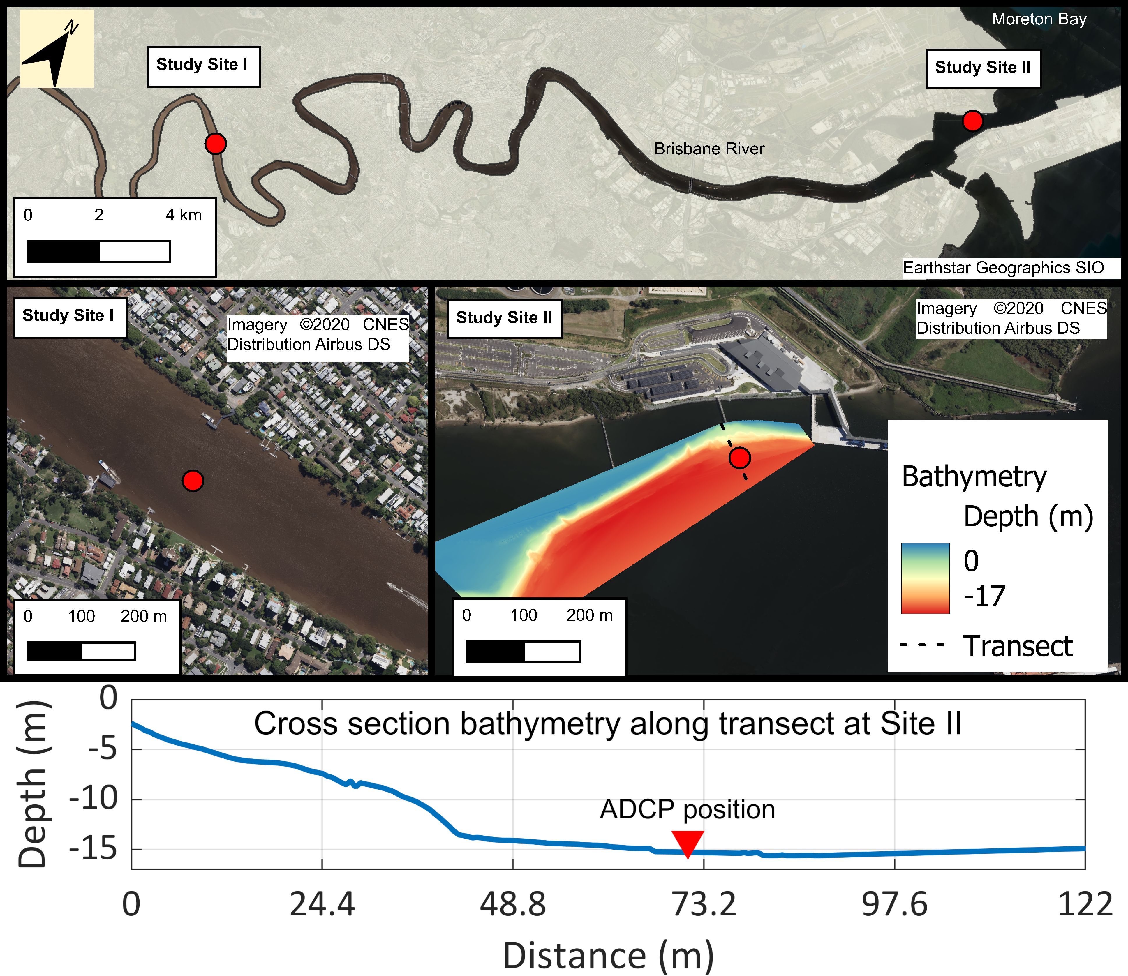
Figure 1. Top panel: Map showing the Brisbane River with Study Sites I and II. Site I: Brisbane River channel near Indooroopilly, Site II: Swing basin inside Brisbane River mouth. Red dots mark the approximate locations of the ADCP moorings. Generated with satellite images from Bing Maps Aerial. Bottom panel: Lateral profile plot of the river bathymetry with the ADCP position marked with a red triangle.

The novel aspect of this work lies in its detailed focus on turbulence dynamics at the mouth of a subtropical estuary fronted by a bay, a setting that has rarely been explored in depth. Flow reversals, observed at slack tide, are shown to have a significant influence on the turbulence regime, driving mixing processes and sediment transport. Unlike previous studies, such as Trevethan et al. (2008), which identified flow reversals in a small creek connected to Moreton Bay, this research examines these phenomena at the estuary mouth, considering their effects across the entire water column and distinguishing their impact during spring and neap tidal cycles. Furthermore, this study delves into how these flow reversals contribute to the development of the turbulence regime over time, a dimension not addressed in prior work. By extending the analysis beyond point measurements and short-term observations, this research provides a comprehensive understanding of the dynamic interplay between flow reversals, tidal cycles, and turbulence in a highly complex estuarine environment. Additionally, the study site near the mouth in a strongly converging part of the estuary, offers unique insights into the dynamics at play in such systems.

Notably, according to the classification scheme presented by Geyer and MacCready (2014), the Brisbane River falls within a category of estuaries experiencing oscillations between strain-induced periodic stratification (SIPS) and well-mixed conditions, a category that remains under-researched in existing scientific literature. The present findings offer a solid basis for understanding turbulence dynamics, particularly the influence of flow reversals and complex estuarine geometry and can be used to characterize turbulence in other heavily modified subtropical estuaries.

2 Materials and methods

A variety of instruments assessing the hydro- and morphodynamic of the study area were deployed during the field campaigns. The ADCPs as the core instruments demand further explanation which is provided in this section. Later on, the study sites are introduced, an overview of the instrumentation is given and the main concepts for the data analysis are presented.

Two methods are typically used to calculate turbulence parameters from the velocity measurements of an ADCP – the variance method and the structure-function (Wiles et al., 2006; Rusello and Cowen, 2011). The variance method is mainly used to calculate Reynolds stresses from the variance of velocity fluctuations in opposing beams, while the structure-function is utilized to assess the dissipation of TKE. The resulting parameterization of turbulence allows insights into the temporal and spatial occurrence and into the strength of mixing processes. Especially the mixing processes are difficult to predict and require field measurements or numerical modeling. For instance, Ralston et al. (2010) demonstrated how much the conditions in a partially stratified estuary can vary and that additional modeling is needed to properly quantify the processes. For the analysis, we utilized the variance technique on the measured ADCP data to calculate Reynolds stresses and TKE following Lohrmann et al. (1990) and Dewey and Stringer (2007).

The use of a 5-beam ADCP enables the estimation of most components of the Reynolds stress tensor, with the exception of the lateral component $-\overline{u\text{'}v\text{'}}$. Often in coastal flows, the lateral component is considered negligible based on the assumption that horizontal length scales significantly exceed vertical length scales (Burchard, 2002; Burchard and Hofmeister, 2008). Consequently, the lateral contribution to the tensor is typically deemed inconsequential. The tensor itself can be represented as follows:

$$\frac{\mathit{\text{τ}}}{\rho }=\{\begin{array}{ccc}-\overline{\mathit{\text{u}}{\text{'}}^{\mathbf{2}}}& -\overline{\mathit{\text{u}}\text{'}\mathit{\text{v}}\text{'}}& -\overline{\mathit{\text{u}}\text{'}\mathit{\text{w}}\text{'}}\\ -\overline{\mathit{\text{u}}\text{'}\mathit{\text{v}}\text{'}}& -\overline{\mathit{\text{v}}{\text{'}}^{\mathbf{2}}}& -\overline{\mathit{\text{v}}\text{'}\mathit{\text{w}}\text{'}}\\ -\overline{\mathit{\text{u}}\text{'}\mathit{\text{w}}\text{'}}& -\overline{\mathit{\text{v}}\text{'}\mathit{\text{w}}\text{'}}& -\overline{\mathit{\text{w}}{\text{'}}^{\mathbf{2}}}\end{array}\}$$

2.1 Study sites

The Brisbane River is situated in South East Queensland, Australia, and meanders over 344 km before emptying into Moreton Bay. Near the mouth of the river, the Port of Brisbane is located and includes several cargo and passenger terminals. Currents in the river at long pocket (35 km upstream of the mouth) reach 0.6 m s^-1 during the flood and ebb tide near the surface. The maximum tidal range lies at 2.7 m during spring tides and 0.7 m during neap tides. Occasionally, substantial rainfall in the catchment area leads to floods and the river carrying large amounts of sediment. The hydrological conditions of the Brisbane River are shaped by seasonal rainfall, flood events, and human interventions. Floods, typically occurring during the summer months due to cyclonic activity and monsoons, can happen year-round. During the study period of October and November, the catchment typically receives moderate rainfall as the wet season begins, with rainfall in the range of 70-100 mm in November. Water extraction for Brisbane City at the Mt Crosby Weir reduces freshwater inflows at the tidal limit to about 1 m³ s^-1, which is significantly smaller compared to the magnitude of tidal flows (Nielsen, 2019).

The maximum depth of the river along its course is 15 meters, a condition largely attributable to extensive dredging activities conducted over the past century. This ongoing dredging and deepening of the estuary have extended the reach of tidal influence to a distance of 80 km from the sea, as documented by Davie and Stock (1990). The mass of dredged material from within the port and navigational channels between November 2016 and February 2017 amounted to 175,000 tons. Dredged material from within the port’s facilities consists mostly of fine silts and clays (D₅₀ = 5 µm). Two study sites were identified, one 35 km upstream of the mouth (site I) and a second site located in the swing basin near the mouth of the river (site II). The sites were selected to investigate the variance in Reynolds stress profiles between the more channelized flow in the middle reach and the complex conditions near the mouth of the estuary. For study site II, the selection was also influenced by the permissions granted by the port authorities, thereby limiting our choice to this specific location. The substrate at site II was investigated for its particle size distribution (PSD) by collecting sediment cores and analyzing them with a Malvern Panalyticial Mastersizer 2000. The PSD is an important characteristic of estuarine study sites. Different bed compositions have different roughness coefficients, affect shear stress, and drag at the bed-fluid interface. Shear stress and drag in turn influence the generation and dissipation of turbulence near the bed.

At site I, an upwards-looking ADCP (Nortek Signature 1000) was installed on the bed close to the middle of the channel, which is 180 m wide. At site II, two upwards-looking ADCPs (RDI Workhorse, Nortek Signature 1000) were installed in the shipping berth of the tanker terminal Port North Common User, situated directly at the mouth of the Brisbane River (Figure 1). The ADCPs were positioned on the channel bed, near the channel bank, as illustrated in the bottom panel of Figure 1. Due to man-made manipulations, the form of the inlet is unique. Fisherman Island, a reclaimed area, forms the eastern part of the river mouth and hosts large parts of the port’s facilities. Between Fisherman Island and the mainland, there is a second inlet to the river with a depth of 1-2 m. Furthermore, after an initial narrow section, the inlet widens again. Depth-averaged flow velocities in the location of the ADCP were limited to 0.4 m s^-1 at maximum.

2.2 Instrumentation

Table 1 lists the locations and settings of the acoustic instruments used during the deployment periods at sites I and II (Figure 2). This setup was aimed at providing data with a high temporal and spatial resolution while minimizing instrument noise. To obtain reliable data, the expected noise level should be substantially lower than the range in which the turbulent fluctuations are assumed to be found. Due to constraints in the availability of the instrument, the measurements at site II took place before the instruments were installed at site I. The tidal range in the mouth of the river during the deployment period between the 08/30/2017 and the 09/28/2017 was found to be 0.55 m at the minimum and 2.23 m at maximum. The bed at site I was comprised of a harder substrate, i.e., sand and pebbles, which allowed the ADCP to be positioned at a tilt of 2.5° pitch and 0.2° roll. This deployment yielded six hours of usable data. At site II, a Nortek Signature (1000 kHz) and an RDI Sentinel Workhorse (600 kHz) were installed. This setup was aimed at providing a comparison between the different generations of devices, reliable measurement of the mean current and high-frequency data for the estimation of turbulence parameters. The usable data from the deployment of the Nortek Signature covered nine days. To guarantee low amounts of tilt which are necessary in order to increase the precision of the measurements, the position and leveling of the ADCP were verified by divers. Additionally, the equation presented by Dewey and Stringer (2007) was implemented in our data processing to remove any remaining influence of tilt on the Reynolds stresses. This further enhanced the robustness of our analyses. Detailed information on this procedure can be found in the data analysis section.

Table 1

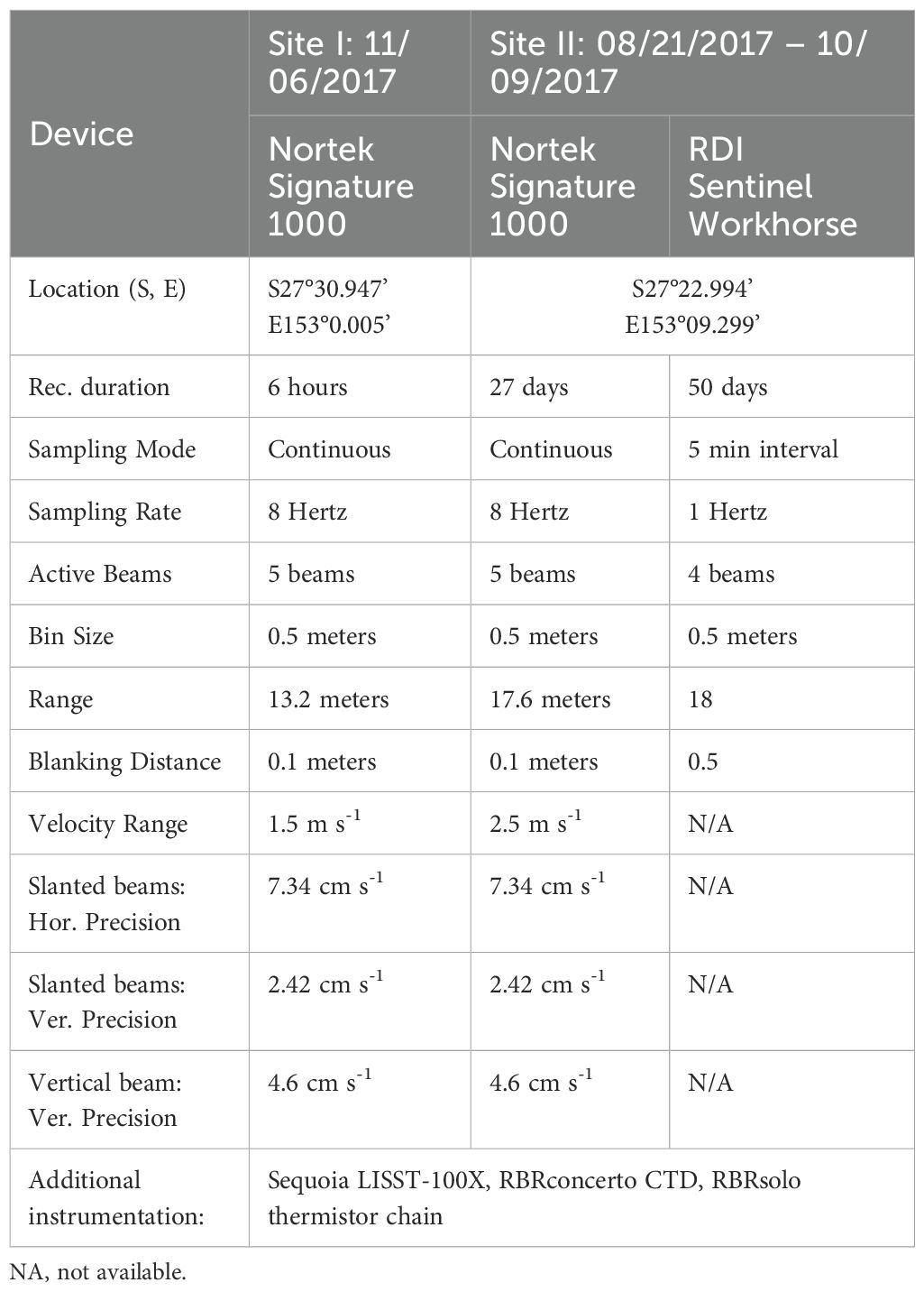
Table 1. Overview of applied instruments at sites I and II.

Figure 2

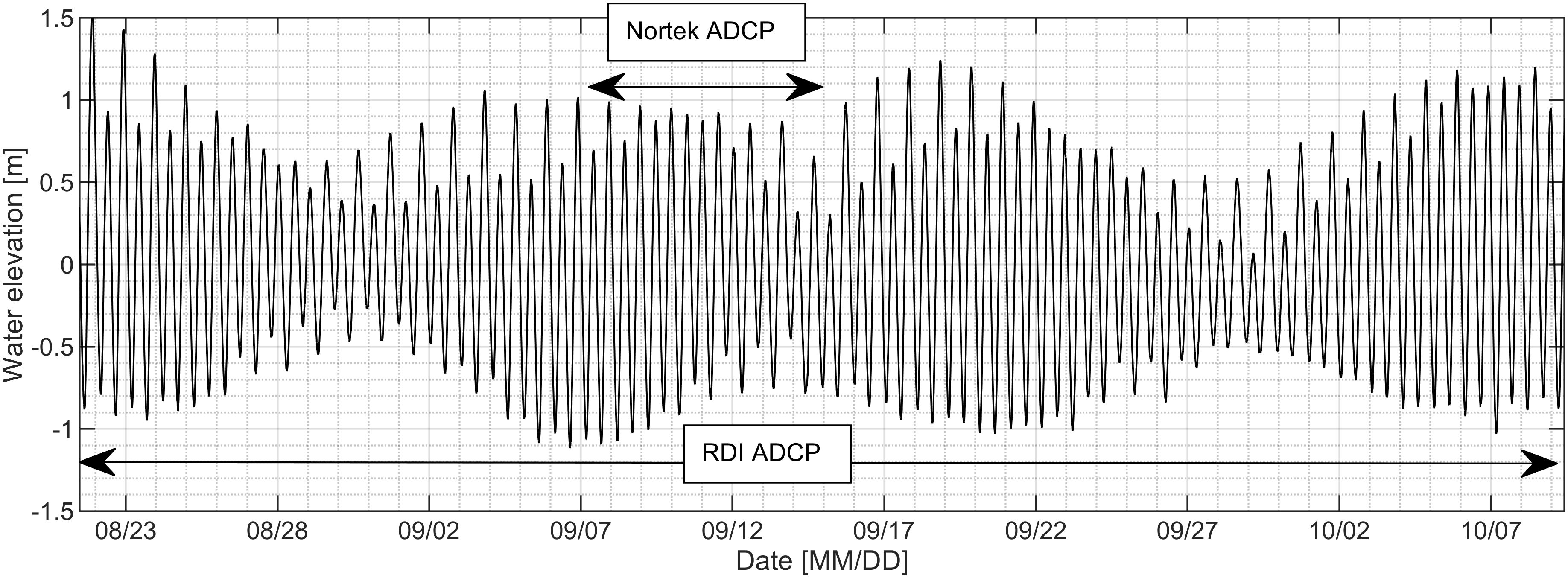
Figure 2. Time series of the water surface elevation from the pressure gauges of the RDI ADCP at site II. Double arrows indicate the deployment lengths of the two ADCPs.

Conductivity, Temperature and Depth (CTD) profile measurements were conducted to assess the possibility of stratification due to the inflowing saltwater during flood tide. On the 09/07/2017 and the 09/14/2017, five down-casts were recorded during a period of six hours on each date. During the deployments on the 09/07/2017 and 09/14/2017, a Laser In-Situ Scattering and Transmissometry instrument (LISST-100X) was installed near the bed for six hours for point measurements of the total volume concentration (TVC) and PSD. Additionally, we installed a chain of nine temperature loggers in close proximity to the ADCPs, which recorded data over the entire study period. The chain was constructed as such that the entire water column was covered, giving insight into the layering inside the column.

2.3 Data analysis

2.3.1 Density calculations

The CTDs measured the salinity using the Practical Salinity Scale. Utilizing the TEOS-10 equation (McDougall and Barker, 2011), density gradients were calculated. To evaluate the contribution of the sediment concentration, it was included in the calculation as follows:

$\begin{array}{ll}\begin{array}{c}\rho ={\rho }_w+\left(1-\frac{{\rho }_w}{{\rho }_s}\right)C\end{array}& (1)\end{array}$

where ${\rho }_w$: seawater density; ${\rho }_s:$ sediment density; C: sediment concentration.

2.3.2 Reynolds stresses

We employed the variance method to estimate the Reynolds stresses and total TKE budget from the velocity measurements. Instead of relying on direct correlations of velocity components, this approach leverages the statistical properties of the flow, allowing it to account for and mitigate the challenges posed by the inhomogeneous nature of flow components (Dewey and Stringer, 2007). Even in shallow waters, e.g., water depth of 15 meters, the topmost measured bins in opposing beams will be several meters apart. When a turbulence field passes through the sensing volume of the ADCP, it is likely that the turbulent motions in different beams stem from different turbulent structures. Thus, the variance method operates on the statistical properties of the raw velocity measurements, that are oriented in the direction of each beam. Even with non-homogenous turbulent flow between diverging beams, the statistical properties remain consistent across the flow field. This method has been effectively employed in multiple studies for the study of turbulence (Milne et al., 2013; Bakhoday-Paskyabi et al., 2018; Imamura et al., 2018; Greenwood et al., 2019; Sentchev et al., 2021; Zippel et al., 2021).

The following equations describe the process for the estimation of Reynolds stresses. Note that a prime ($x\text{'}$) denotes the fluctuating part and an overbar ($\overline{x}$) the time-averaged component which is established over a period in which the flow stays quasi-stationary. In tidal flows, this period has been identified to be in the range of 8 – 12 minutes (Soulsby, 1980).

The variance method used for this work was formulated by Dewey and Stringer (2007) for a 5-beam ADCP as follows. $\overline{u^{\prime }{w}^{\prime }}$ was calculated from the averaged velocity fluctuations of the opposing beam 1 and beam 2. $\overline{v^{\prime }{w}^{\prime }}$ was calculated from the averaged velocity fluctuations of the opposing beam 3 and beam 4:

$\begin{array}{ll}\begin{array}{c}-\overline{u^{\prime }{w}^{\prime }}=\frac{\overline{b_2^{\prime 2}}-\overline{b_1^{\prime 2}}}{2\sin 2\theta }\end{array}& (2)\end{array}$

where $\overline{u^{\prime }{w}^{\prime }}$: streamwise Reynolds stress; b_i: radial velocity in beam I; θ: elevation angle.

$\begin{array}{ll}\begin{array}{c}-\overline{v^{\prime }{w}^{\prime }}=\frac{\overline{b_2^{\prime 2}}-\overline{b_1^{\prime 2}}}{2\sin 2\theta }\end{array}& (3)\end{array}$

where: spanwise Reynolds stress; b_i: radial velocity in beam I; θ: elevation angle. $\overline{v^{\prime }{w}^{\prime }}$ in case of instrument tilt, was calculated from the averaged velocity fluctuations of the opposing beam 1 and beam 2. $\overline{u^{\prime }{w}^{\prime }}$ in case of instrument tilt, was calculated from the averaged velocity fluctuations of the opposing beam 3 and beam 4:

$\begin{array}{ll}\overline{u^{\prime }{w}^{\prime }}=\frac{-1}{4{\sin }^6\theta {\cos }^2\theta }\left\{\begin{array}{l}{\sin }^5\theta \cos \theta (\overline{b_2^{\prime 2}}-\overline{b_1^{\prime 2}})+2{\sin }^4\theta {\cos }^2\theta {\phi }_3(\overline{b_2^{\prime 2}}+\overline{b_1^{\prime 2}})\\ -4{\sin }^4\theta {\cos }^2\theta {\phi }_3\overline{b_5^{\prime 2}}-4{\sin }^6\theta {\cos }^2\theta {\phi }_2\overline{u^{\prime }{v}^{\prime })}\end{array}\right\}& (4)\end{array}$

where $\overline{u^{\prime }{w}^{\prime }}$: streamwise Reynolds stress; b_i: radial velocity in beam I; θ: elevation angle; φ_1,2,3: heading, pitch, roll.

$\begin{array}{ll}\overline{v^{\prime }{w}^{\prime }}=\frac{-1}{4{\sin }^6\theta {\cos }^2\theta }\left\{\begin{array}{l}{\sin }^5\theta \cos \theta (\overline{b_4^{\prime 2}}-\overline{b_3^{\prime 2}})+2{\sin }^4\theta {\cos }^2\theta {\phi }_3(\overline{b_4^{\prime 2}}+\overline{b_3^{\prime 2}})\\ -4{\sin }^4\theta {\cos }^2\theta {\phi }_3\overline{b_5^{\prime 2}}-4{\sin }^6\theta {\cos }^2\theta {\phi }_3\overline{u^{\prime }{v}^{\prime })}\end{array}\right\}& (5)\end{array}$

where $\overline{v^{\prime }{w}^{\prime }}$: spanwise Reynolds stress; b_i: radial velocity in beam I; θ: elevation angle; φ_1,2,3: heading, pitch, roll.

The total kinetic energy budget including a correction for possible tilt of the device is calculated as follows:

$\begin{array}{ll}\begin{array}{c}\frac{q^2}{2}=\frac{1}{4si{n}^2\theta }\{\overline{((b_1^{\prime 2})}+\overline{b_2^{\prime 2}}+\overline{b_3^{\prime 2}}+\overline{b_4^{\prime 2}})-2(2{\cos }^2\theta )\overline{b_5^{\prime 2}}-(cot\theta -1){\phi }_3\left(\overline{b_2^{\prime 2}}-\overline{b_1^{\prime 2}}\right) \end{array}& (6)\end{array}$

where q: total kinetic energy; b_i: radial velocity in beam I; θ: elevation angle; φ_1,2,3: heading, pitch, roll.

Further processing was done in MATLAB to ensure the quality of the data. For this purpose, the amplitude and correlation computed by the instruments were used. The amplitude is a parameter computed by the ADCP that represents the strength of the reflected signal, while the correlation is a measure of how similar the reflected signal is to the signal that was emitted. The amplitude decreases with distance from the instruments and therefore a lower threshold was used to remove measurements where the amplitude falls below the noise level of the instrument. The correlation also declines with distance from the instrument and represents a quality measure of the velocity measurements. A quality control filter with standard criteria recommended by RDI (Amplitude > 30 dB, Correlation > 50%) and Nortek (Correlation > 50%) was used to clean the data and remove faulty or inaccurate measurements. RDI provides clear and explicit criteria in their principle of operation for both amplitude and correlation, while Nortek only specifies a correlation threshold of 50%, with no fixed amplitude criteria in their articles on quality control. Instead, Nortek recommends that the signal should be at least 3 dB higher than the noise floor, which was applied during post-processing using Nortek’s Signature Viewer. To correct for possible erroneous measurements due to outliers caused by air entrainment or objects in the water column, such as fish, that interfere with the propagation of the acoustic signal, we applied a kernel-density-based despiking method to the velocity measurements in each bin collected by the ADCP (Islam and Zhu, 2013). The despiking method systematically identified and removed outliers attributed to such sources while preserving the integrity of valid data. Following the authors recommendations and code (Islam, 2024), we used suggested bandwidth values of hx = 0.01 and hy = 0.01 for the kernel density estimation. Identified spikes were replaced by linearly interpolated values to reconstruct the time series. The percentage of pings removed during the despiking process was minimal: beam 1, 0.13 percent; beam 2, 0.05 percent; beam 3, 0.09 percent; beam 4, 0.07 percent; and beam 5, 0.12 percent. These low removal rates indicate a high-quality dataset, consistent with our initial visual inspection. We attribute this robustness to the relatively shallow water depth, large bin size, and the high turbidity of the water, which reduces the likelihood of signal contamination or spurious data. This approach further reinforces the validity of our turbulence measurements and subsequent analyses.

Data influenced by sidelobe interference was removed as well by identifying spikes in the amplitude data and limiting the range of the ADCP to exclude these data points. The calculation of Reynolds stresses started with the Reynolds decomposition into the mean and fluctuating part (averaging period = 10 min). The primary directions of flood and ebb currents were ascertained through flow direction data obtained from the ADCPs. The major axes characterizing the flow were also established. Subsequently, the flow velocities were decomposed into their longitudinal (u) and lateral (v) components. Vertical (w) velocities were captured using the data from the fifth beam, oriented vertically. After applying the variance method and determining the main flow direction, the stresses were rotated into the stream- and spanwise flow direction. Finally, the parameters were averaged over 10 and 60 minutes to display ensemble-averaged features during the tidal cycle. Averaging also reduces errors that arise from the random noise inherent to acoustic measurements.

2.3.3 Turbidity to suspended Solids calibration

From several field measurements conducted in the swing basin by the Port of Brisbane (Richardson et al., 2017), where study site II was located, the relation of turbidity measured in the Nephelometric Turbidity Unit (NTU) to Total Suspended Solids (TSS) was calculated and used in this study. As this relation is only valid for the specific relation found at site II, the conversion was not attempted for the CTD measurements from site I.

$\begin{array}{ll}\begin{array}{c}y=2.8413x+18.036\end{array}& (7)\end{array}$

where y: total suspended solids; x: turbidity (NTU).

2.3.4 Turbulence and mixing quantities

The gradient Richardson number (Ri_g) highlights the balance between stratifying forces and the potential for shear-driven mixing in a flow. A value of Ri_g< 0.25 indicates conditions favorable for shear driven mixing, while Ri_g > 0.25 points to the dominance of stratifying influences. It is given as:

$\begin{array}{ll}R{i}_g= -\frac{g}{{\rho }_0}\frac{\frac{\delta \rho }{\delta z}}{{(\frac{\delta u}{\delta z})}^2} & (8)\end{array}$

and can be rewritten as $R{i}_g=\frac{N²}{S²}$. In estuarine settings, the buoyancy frequency (N²) is pivotal for understanding the stability of the water column and is calculated using the equation.

$\begin{array}{ll}{N}^2= -\left(\frac{g}{\rho }\right)\left(\frac{d\rho }{dz}\right)& (9)\end{array}$

The buoyancy flux B informs us about the amount of turbulent kinetic energy (TKE) which acts to mix buoyancy and is given by

$\begin{array}{ll}B=\frac{g}{{\rho }_0}\overline{{\rho }^{\prime }{w}^{\prime }}& (10)\end{array}$

We calculate density using the thermistor chain data, as it closely correlates with density derived from salinity and temperature (see Supplementary Figure 1) and offers an extended time series compared to CTD profiles. Shear velocity u* is a useful parameter for estimating bed shear stress, contributing to sediment transport and resuspension; its equation is

$\begin{array}{ll}{u}^{*}=C_D{U}_{max}& (11)\end{array}$

The Potential energy anomaly (PEA), defined by Simpson in 1981, is crucial for understanding the energy changes in stratified water columns, and its equation is:

$\begin{array}{ll}\phi ={\displaystyle {\int }_{-H}^0(\rho -{\rho }_0)gzdz} & (12)\end{array}$

It provides a measure of how much energy would be needed to return a stratified water column to its fully mixed state. The Simpson or horizontal Richardson number Si serves as a measure to gauge the balance between buoyant and inertial forces in the estuary, and its equation is:

$\begin{array}{ll}Si=\frac{b_x{H}^2}{C_D{U}_T^2}& (13)\end{array}$

It serves as a parameter with which estuaries can be classified on a range from fully mixed to stratified. The vorticity ω_x is a measure of lateral circulation in estuaries, and it aids in understanding secondary flows; its equation is

$\begin{array}{ll}{\omega }_x=\delta w/\delta y-\delta v/\delta z& (14)\end{array}$

Lastly, eddy diffusivity quantifies vertical mixing in the water column and is calculated as:

$\begin{array}{ll}{K}_z=\frac{ϵ}{N^2}& (15)\end{array}$

, where ϵ is the TKE dissipation rate and N² is the buoyancy frequency as described above. The dissipation rate ϵ is estimated using a dimensional analysis approach, assuming a balance between turbulent energy production and dissipation (Taylor, 1935):

$\begin{array}{ll}ϵ=C_{ϵ}\frac{q_0^3}{l}& (16)\end{array}$

here Cϵ is an empirical constant (0.19), q is the computed TKE, and l is the mixing length scale, set to 15 m in this study, set to the mean of the computed length scales at study site II.

Where ${\rho }_0$: reference density; $\rho$: density; g: gravitational acceleration; u: longitudinal velocity; v: lateral velocity; w: vertical velocity; s: salinity concentration; H: water depth; C_d: drag coefficient; U_max: maximal flow velocity; b_x: horizontal buoyancy gradient; U_t: tidal flow velocity (depth averaged maximum velocity).

2.3.5 Integral time and length scales

The description of turbulence often refers to the time and length scale of its features to characterize the turbulent motions. To assess these scales, an autocorrelation function is used. The integral time scales can be found by calculating the correlation of turbulent motions with themselves (Equation 17), identifying the point where the function becomes uncorrelated and integrating the calculated autocorrelation coefficient function (Kundu et al., 2016).

$\begin{array}{ll}\begin{array}{c}{T}_i={\displaystyle {\int }_{\tau =0}^{\tau (R_{ii}(\tau )=0)}{R}_{ii}(\tau )d\tau }\end{array}& (17)\end{array}$

where R_ii: autocorrelation function; τ: time lag.

By assuming Taylor’s hypothesis of frozen turbulence that eddies are rigid when passing through the sensing volume of the ADCP, the length of these eddies can be estimated by Equation 18.

$\begin{array}{ll}\begin{array}{c}{L}_i=u_{i}T\end{array}& (18)\end{array}$

where L: length; u_i: current velocity; T: time.

The estimated length and time scales are the scales found at the upper end of the energy cascade, i.e., from the large eddies carrying the most energy in turbulent flows. Regarding practical applications in coastal/hydraulic engineering, these scales are inferred to be the most important ones as they carry substantial amounts of energy and momentum.

3 Results

3.1 Classification

To facilitate comparison with results from other estuaries, the Brisbane River has been classified based on its dominant tidal constituents and stratification stability. The computation with u_tide (Codiga, 2011) allowed us to identify the most dominant tidal constituents in the area. These are the most dominant constitutes sorted in descending order by their contribution to the tidal fluctuations: M2 (79.82%), S2(9.30%), K1(5.04%), O1(2.52%). They indicated that the tides were mainly driven by the lunar semidiurnal component with smaller contributions from the solar semidiurnal and lunar diurnal component. Tidal variations therefore appeared twice daily, though with differing magnitude. We also found that the alterations in water level resulting from the M2 and S2 tides exhibit delays compared to the occurrence of slack tide, which marks the reversal of the flow. Specifically, a 14.57-degree phase lag corresponded to a time delay of roughly 0.503 hours for the S2 tide, while a 1.95-degree phase lag corresponded to a time lag of approx. 0.067 hours for the M2 tide.

Overtides, including M4 and M6, were also detected. The overtide M4, a harmonic of M2, accounts for 0.05 percent of the total energy, while M6, a higher harmonic of M2 as well, contributes 0.03 percent. These overtides, though small in energy contribution compared to the primary constituents, indicate the influence of nonlinear effects, likely due to shallow water dynamics. These overtides suggest that while the tides are primarily driven by the dominant constituents, nonlinear processes play a subtle yet significant role in the system’s dynamics.

Using the daily tidal form factor (Marées, 1938), the tidal regime was classified as mixed semidiurnal.

$\begin{array}{ll}\begin{array}{c}F= \frac{K_1+O_1}{M_2+S_2}=0.32\end{array}& (19)\end{array}$

In order to characterize the stability if the stratified water columns in the Brisbane River, we have computed the Simpson number. The Simpson number during ebb amounts to 0.02, while it rises to 0.82 during the flood. Several authors have analysed the implications of the Simpson number quantitively. Stacey and Ralston (2005) identified Si ~ 0.2 as the transition threshold during ebb. Values higher than 0.2 indicate permanent stratification while lower values suggest that the entire water column can potentially experience full mixing during ebb tide. According to a quantitative analysis by Becherer et al. (2015), a critical value for Si during flood is 0.84. Lower values indicate that the water column experiences strain-induced periodic stratification (SIPS), while higher values indicate a persistent stratification. Following these guidelines, the Brisbane River was characterized as potentially fully mixed during the ebb flow, while during the flood flow the estuary was experiencing SIPS.

Classifying the river with classification approaches by Hansen and Rattray (1966) and Geyer and MacCready (2014) was not possible due to the dataset being limited to point and profile measurements instead of moving boat measurements, though the variation between SIPS and well mixed would classify it close to the Willapa Bay (Olabarrieta et al., 2011). The observed impact of TKE on the upper water column in the ebb shoal region bears similarities to the hydrodynamic conditions noted in the Brisbane River. In both cases, the injection of TKE contributed to enhanced mixing in the upper layers of the water column. The particle size distribution from bed cores indicated that the substrate of the top 30 - 40 cm of the riverbed largely consists of fine particles, e.g., silt, clay, and colloids.

The framework by Toffolon et al. (2006) allowed us to include the converging nature of the estuary in the classification of our study area, providing a comprehensive understanding of how convergence, friction, and nonlinear effects influence tidal dynamics. The Brisbane River estuary demonstrates characteristics of a strongly convergent system. The dimensionless tidal amplitude is calculated as 0.169, reflecting moderately strong relative tidal influence. The estuary’s convergence length - derived from its width, which decreases from 930 meters upstream to 500 meters at the mouth over 1.6 kilometers - is approximately 2.07 kilometers. This results in a high convergence ratio of 42.98, emphasizing the estuary’s strong geometric narrowing. Coupled with a friction-to-inertia ratio of 0.588, the system is primarily governed by convergence dynamics rather than frictional dissipation.

In the classification framework, the Brisbane River falls into the category of strongly convergent and weakly dissipative estuaries. The dominance of convergence over friction suggests a dynamic system where tidal amplification is likely influenced more by geometry than by energy losses due to friction. These findings are consistent with estuarine behavior commonly observed in systems with significant narrowing and moderate tidal forcing.

3.2 Observations

This chapter focuses on presenting the key findings from the two study sites, with an emphasis on the parameters measured and calculated to investigate their hydrodynamic and turbulence dynamics. While Study Site I exhibited relatively uniform and channelized flow conditions, the situation at Study Site II was more complex. To better understand the dynamics at Study Site II, additional parameters were calculated, including turbulent TKE, eddy diffusivity, N², and buoyancy flux. These calculations were complemented by more extensive measurements, such as data collected using a temperature chain to analyze thermal stratification.

The chapter is divided into focused sections that systematically address general conditions, turbidity and salinity, turbulence dynamics, and the temporal and spatial scales of turbulent structures. Observations at Study Site I are presented first in each section, followed by the more intricate patterns observed at Study Site II. This comparative approach highlights both the similarities and the key differences between the two sites, forming a foundation for the synthesis and broader implications discussed in subsequent chapters.

3.2.1 General conditions

3.2.1.1 Study Site I

The tidal range in the investigated period at study site I was 2 meters, while the flow velocity ranged from 0.26 to 0.72 m s^-1. The ebb stream velocity ranged from 0.1 to 0.7 m s^-1. The flow was uniformly directed upstream during the flood period and uniformly downstream during the ebb period (Figure 3). The flow conditions during the measured flood flow at site I were defined by its channelized structure.

Figure 3

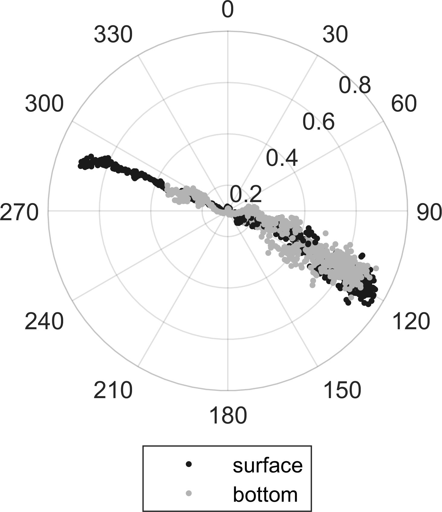
Figure 3. Polar plots of the flow direction at site I (06.11.17 and 15.11.17).

3.2.1.2 Study Site II

The hydrodynamic conditions near the swing basin at site II were more complex and significantly different from observations at site I. Two main flow directions were evident, 10° to 20°for the ebb flow and 190° to 200°from due north for the flood flow. Typically, the flood flow exhibited two flood peaks, reaching 0.45 m s^-1 (Figure 4). Furthermore, lateral velocities exhibited substantial influences, these velocities reached up to 0.1 m s^-1 and displayed distinct patterns where flows in opposing directions were clearly observable in the cross-sectional view. During every second low water the reversal of the flood flow was evident, which persisted for approx. 20 min (Figure 4).

Figure 4

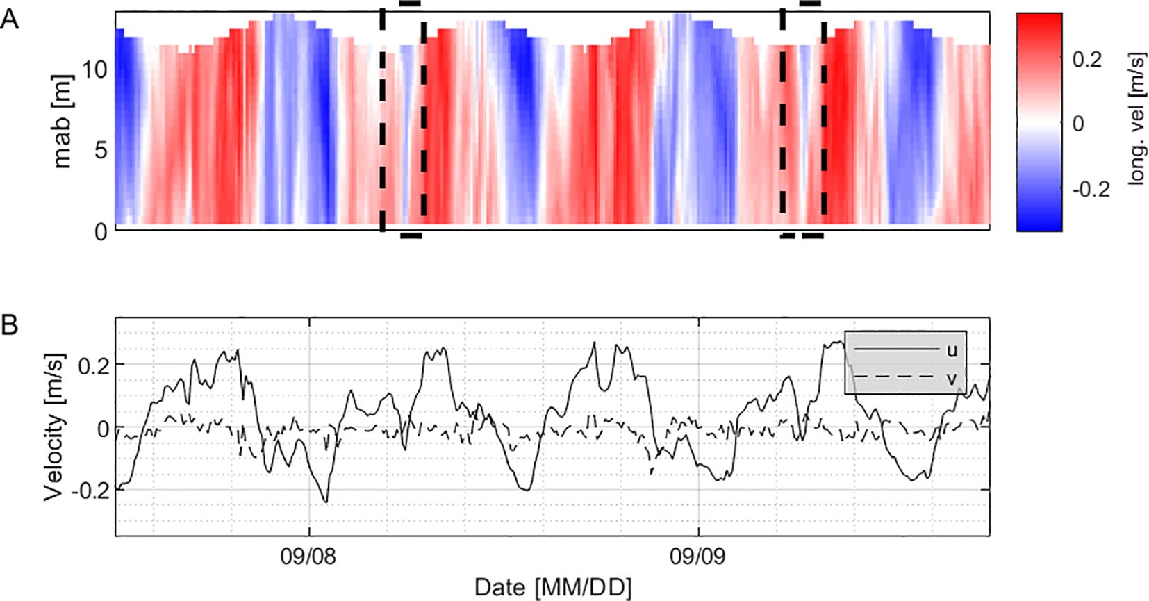
Figure 4. (A) Depth-time evolution of longitudinal velocity, flow reversals marked by the dashed rectangles. (B) Timeseries of u (streamwise) and v (spanwise) depth-averaged velocity at study site II for a 24-hour period starting on the 09/07/2017.

A continuous time series from the Nortek Signature from study site II from the 08/09/2017 to the 09/16/2017 is displayed in Figures 5A–C. The displayed period starts in the middle of a spring-neap cycle and finishes at the end of the cycle. Figure 5A depicts the water speeds during the flood and ebb cycle. The flood and ebb flow reversed their direction well before the water level started rising and falling respectively. During low tide residual velocities which were opposed to the main flow direction were evident. Figure 5B reveals patterns in the lateral velocity measurements. During low tide when the flood started to flow, a circulation pattern was visible. Water near the bottom moved towards the bank, while water near the surface moved in the opposite direction. During the ebb tide the pattern reversed, though the periods over which this was evident were less clearly defined and shorter.

Figure 5

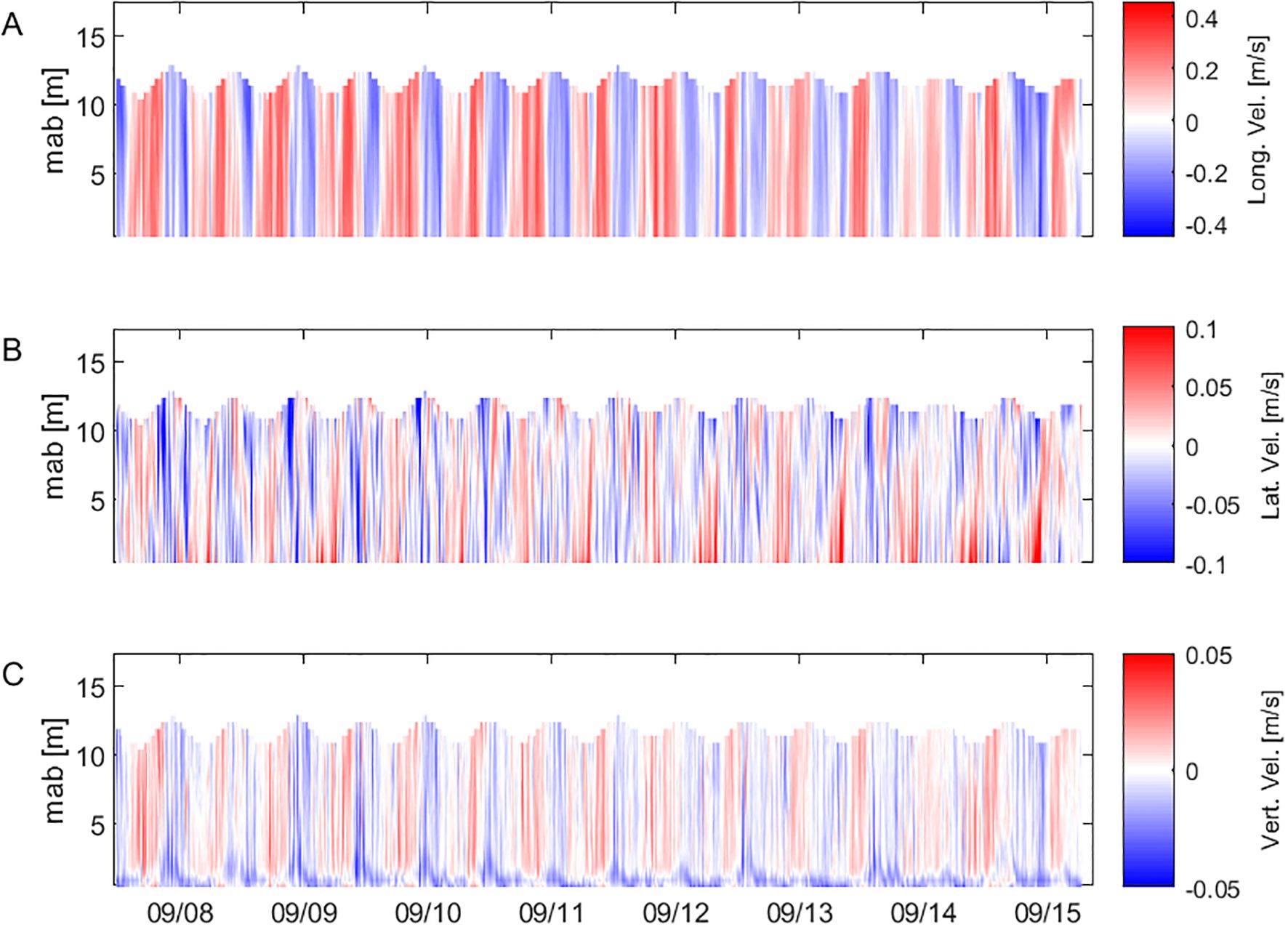
Figure 5. Depth-time evolution of (A) velocity magnitude (negative = ebb) and PEA, (B) lateral velocity, (C) vertical velocity.

The vertical velocities as depicted in Figure 5C show that the flood was accompanied by upwards moving velocities, while ebb was accompanied by downward moving velocities. The general vertical movement of the water was probably due to the Brisbane bar being approx. 2 km upstream of the study site forcing the flood flow into upwelling and ebb flow into downwelling. During high and low tide, there were periods of alternating velocities evident. The flow in close proximity to the riverbed exhibited significant disparities compared to the flow throughout the remainder of the water column. Near the bed at a distance of 0.4 m to 1.9 m from the bed, a layer of downward directed currents was evident that persisted through the ebb and flood tide. During the ebb tide, this layer grew in thickness and occupied the entire water column. Though the measured velocities were small and might in part have been smaller than the measurement uncertainty of the ADCP, we believe them to be accurate. Both ADCPs exhibited similar velocity structures, although some variability was observed. The vertical velocities as measured by the second ADCP (RDI) are displayed in Supplementary Figure 2. These small discrepancies between the two devices could be attributed to differences in measurement uncertainty as well as variations in their internal processing algorithms.

Additionally, the estimation of the N² (Figure 6B) demonstrated a layer with high oscillating frequencies near the bed in the same region. The buoyancy frequencies were estimated solely from the temperature chain measurements and therefore they were independent of any contamination by the measurement errors in the ADCP data.

Figure 6

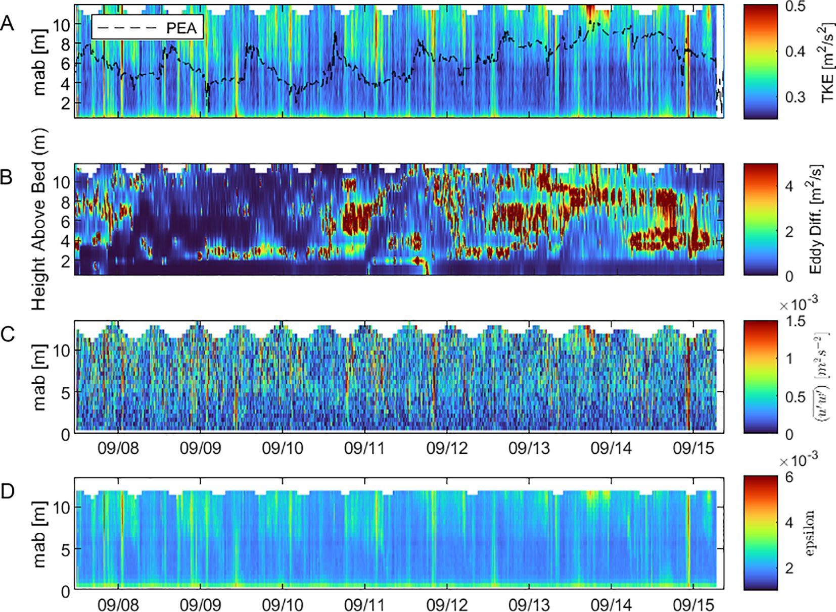
Figure 6. Depth-Time evolution of (A) total TKE budget and PEA, (B) Eddy Diffusivity, (C) Reynolds stresses ($\overline{u\text{'}w\text{'}}$), (D) dissipation rate.

3.2.2 Turbidity and salinity

3.2.2.1 Study Site I

Turbidity and salinity profiles taken on the 11/06/2017 during a flood tide revealed that the water column was well mixed and that the salinity increased with the flood flow to 17 PSU (Figure 7). The profiles indicated that the turbidity rose to 26 NTU during flood tide and then notably dropped to 22 NTU upon reaching slack tide at high water, when the flow began to reverse direction. The measurements taken during high tide indicated a significant decrease in turbidity levels at mid-depth, while the turbidity near both the surface and the bed remained consistent with previous measurements.

Figure 7

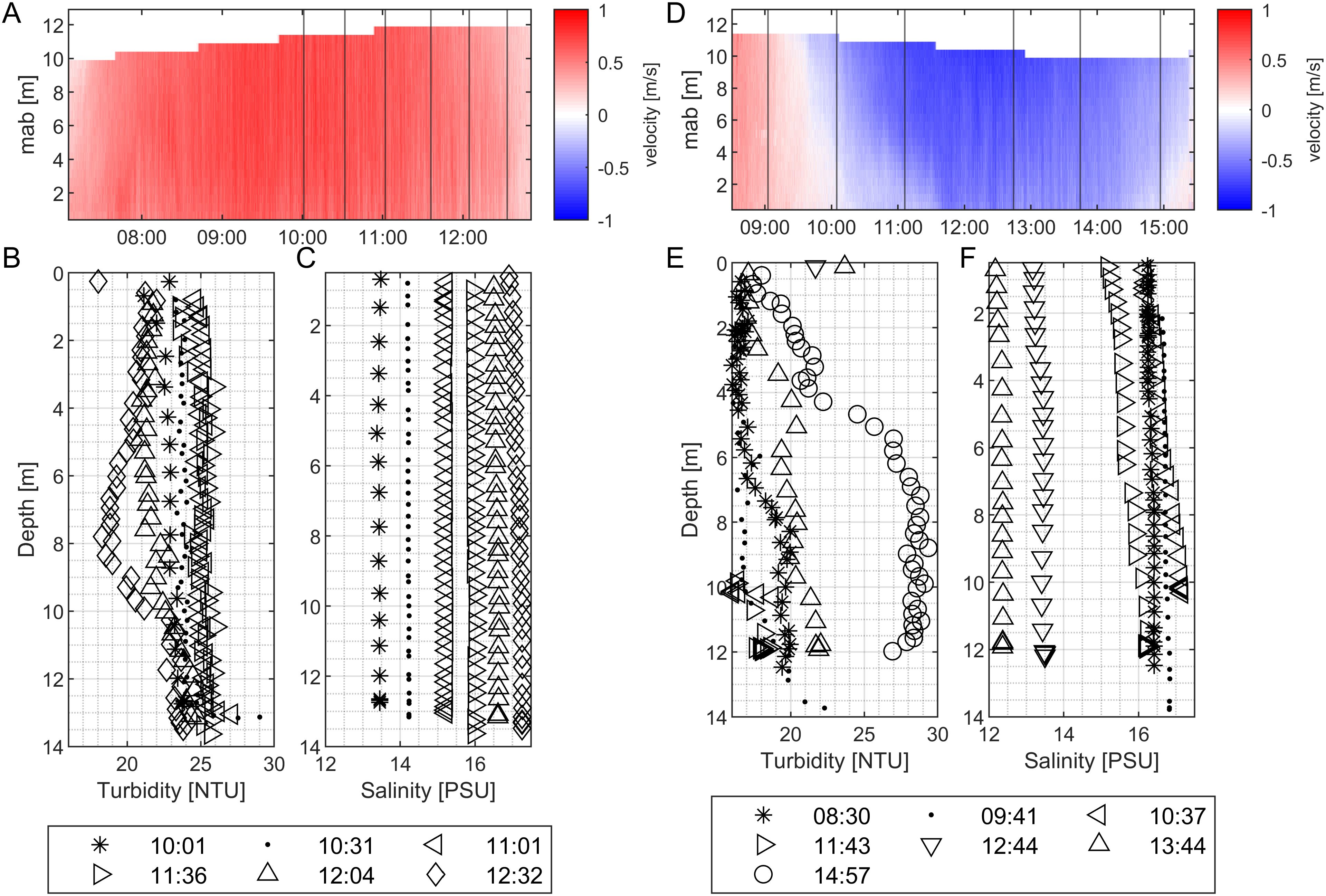
Figure 7. Data from the CTD from the 11/06/2017 of (A) black line indicating the water elevation with black stars marking the CTD profiling times corresponding to the times in the lower plots, (B) turbidity and (C) salinity. Data from CTD from the 11/15/2017 of (D) black line indicating the water elevation with black stars marking the CTD profiling times corresponding to the times in the lower plots, (E) turbidity and (F) salinity.

CTD Profiles from an ebb tide on the 11/15/2017 demonstrated that the water column was well mixed although there was a salinity gradient evident with increasing salinity towards the bed (Figure 7). During ebb tide, the salinity steadily decreased from approx. 17 to 11.5 PSU. The turbidity remained constant during large parts of the ebb tide and only started to increase during the last 2 hours approaching low tide when an increase in turbidity was evident over the entire water column and most pronounced near the bed.

3.2.2.2 Study Site II

The salinity profiles from study site II show less saline water near the water surface at high tide. During the following measurements at ST+2h, the water column stratified with a distinct interface forming at a depth of 6 meters. The gradient in salinity was still evident at ST+3h but less prominent. On the 09/14/2017 the data shows three clear peaks in TVC (µL L^-1), shortly before low tide, during low tide, and shortly after low tide (Figure 8). The measurements of the vertical turbidity gradient displayed several peaks in turbidity with up to 50 mg l^-1 shortly after low tide in the upper half of the water column. The salinity during low tide seemed well mixed, while the water column was stratified at ST+1h and in the following measurements due to the inflowing flood tide.

Figure 8

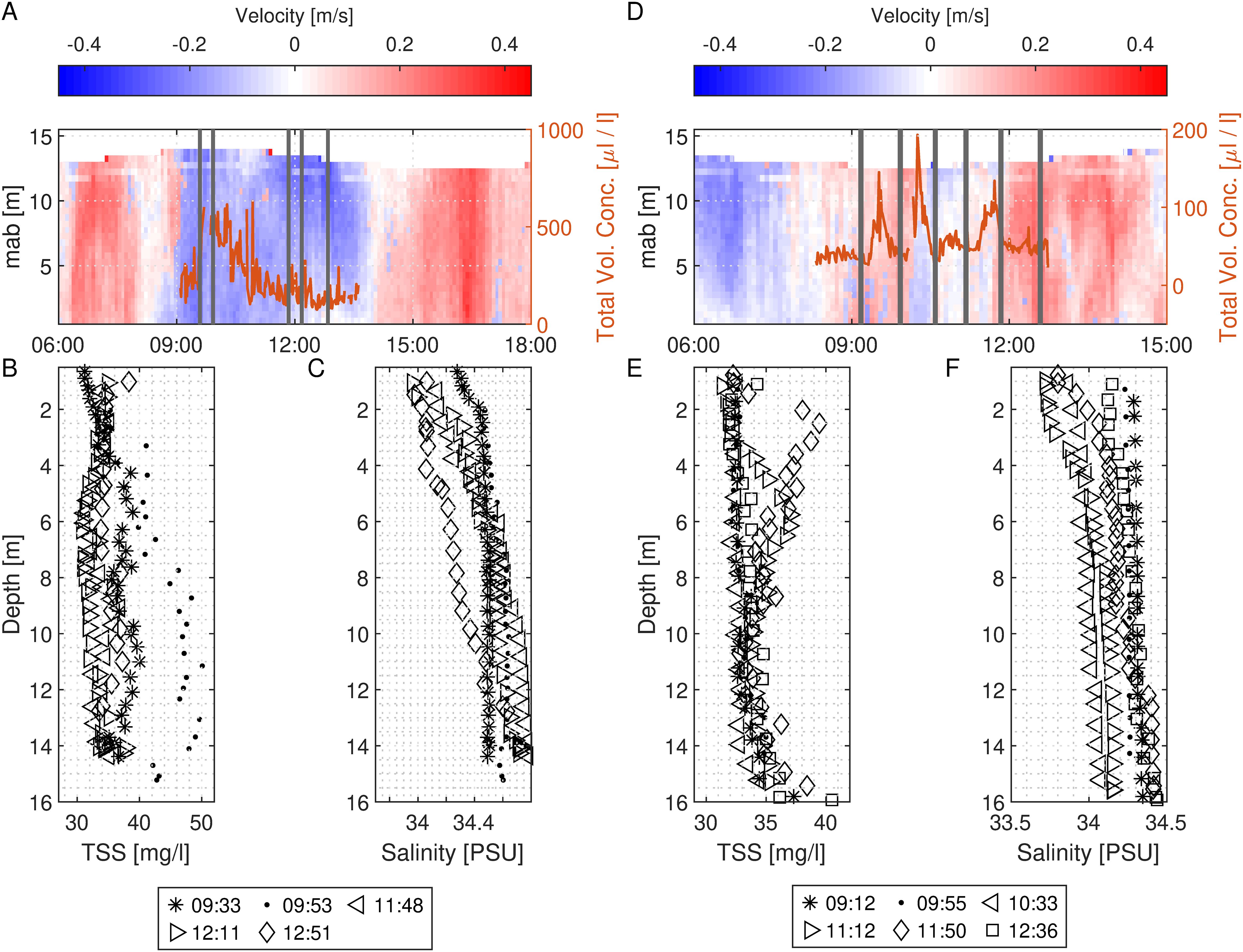
Figure 8. Data from CTD and LISST from the 09/07/2017 of (A) Depth time evolution of flow velocity: black horizontal lines indicating the CTD profiling times corresponding to the times in the lower plots, the brown line indicating the total volume concentration from the LISST, (B) density and (C) salinity. Data from CTD and LISST from the 09/14/2017 of (D) suspended sediment, (E) density and (F) salinity.

Point measurements of the TVC at study site II with a LISST-100X were conducted during high tide and the following ebb tide on the 09/07/2017 and during low tide and the following flood tide on the 09/14/2017 (Figure 8). The data collected on 09/07/2017 indicated that both turbidity and TVC reached peak levels during high tide as ebb flow commenced, with elevated turbidity observed near the seabed. Subsequently, both TVC and turbidity diminished during the following ebb tide and appeared to be uniformly distributed throughout the water column.

3.2.3 Reynolds stress profiles

3.2.3.1 Study Site I

The Reynolds stress profiles at study site I over the water column and the corresponding flow velocities during the averaging periods are depicted in Figures 9A and B. Turbulence was generated near the bed and decreased with distance to the bed, approaching values near zero at the water surface. The magnitude of stresses correlated with the mean velocity profiles (Figure 9B). Stress grew from the bottom upwards during slack tide (ST), ST+1h and ST+2h, while the measurements taken at ST+3h and ST+4h displayed the maximum stress profiles. At ST+5h the stresses fell back to levels found during the increasing flood flow. All profiles except the ST and ST+1h displayed a rapid decrease in stresses near the bed, in accordance with common boundary layer theory where velocity gradients and therefore stresses reduce to zero.

Figure 9

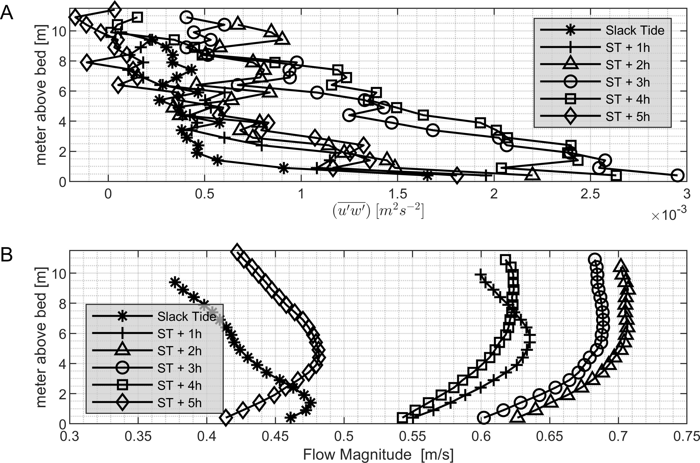
Figure 9. (A) Reynolds stresses during the flood tide on the 11/15/017 in averaging intervals of 60 minutes, (B) Corresponding 60-minute averages of the flow magnitude in m s^-1.

3.2.3.2 Study Site II

The estimated streamwise Reynolds stresses from the deployment near the mouth of the river covered a period of nine days. The entire time series was phase-averaged over every 1st and 2nd tide to form stress profiles that can be compared. The averaged Reynolds stress profiles for successive first and second tides exhibited distinct characteristics, as illustrated in Figure 10. In the first tide, represented by blue curves in Figures 10A and B, with corresponding flow velocities in Figure 10C, the Reynolds stresses were considerably lower in the upper water column during both flood and ebb phases. However, during the high-water stage, there was a pronounced increase in ($\overline{v^{\prime }{w}^{\prime }}$) stresses near the seabed. In contrast, the second tide, depicted by red curves in Figures 10A, B, D, demonstrates substantial ($\overline{v^{\prime }{w}^{\prime }}$) stresses near the water surface during the flood and ebb stages, while these stresses diminished to nearly zero at high water. The ($\overline{u^{\prime }{w}^{\prime }}$) stress profiles were less consistent, making it challenging to identify clear patterns. Nevertheless, ($\overline{u^{\prime }{w}^{\prime }}$) stresses tended to be higher during the flood and ebb phases of every first tide, as indicated by the blue profiles.

Figure 10

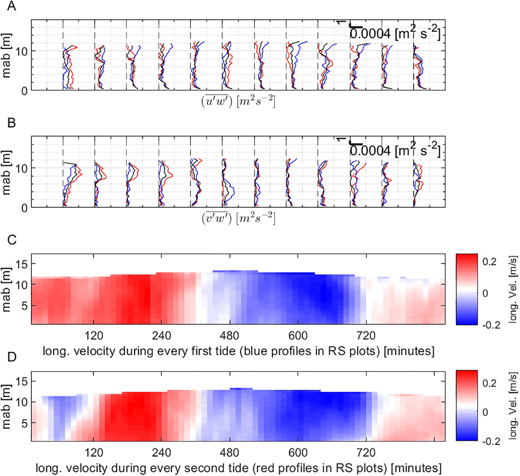
Figure 10. (A) Profiles of Reynolds stresses, phase-averaged over the 10 recorded tidal cycles at site II. Blue: during every first tide, (B) red: during every second, black: average of all tides. (C) corresponding phase-averaged horizontal velocity during every first tide, (D) during every second tide.

3.2.4 PSD

3.2.4.1 Study Site I

Figure 11A depicts the power density spectrum of the turbulent fluctuations formed with Welch Overlapped Segment Averaging (WOSA). We used streamwise horizontal velocity fluctuations for the calculation. The different lines in the figure represent the PSD in each bin from the ADCP. The spectrum was calculated over 60-minute parts divided into 50-second segments with an overlap of 50% and a von-Hann data taper. The data for the spectrum in the figure was taken from a 60-minute period during peak flood flow at site I. The frequency range in which the spectra displayed the expected slope was found between 0.1 Hz< f< 0.9 Hz. At higher frequencies, noise superimposes any turbulent features and therefore also masked the energy cascade towards dissipation at the smallest scales. The spectral noise level was evident at S(f) = 10^-4m²s^-2Hz^-. During the peak flood velocity, the f^-5/3-slope was quite clear in the isotropic span between the production and the dissipation range. This confirmation aligns our data with established turbulence theory, specifically Kolmogorov’s predictions, underscoring the robustness of our measurement techniques and assuring readers of the reliability of our data.

Figure 11

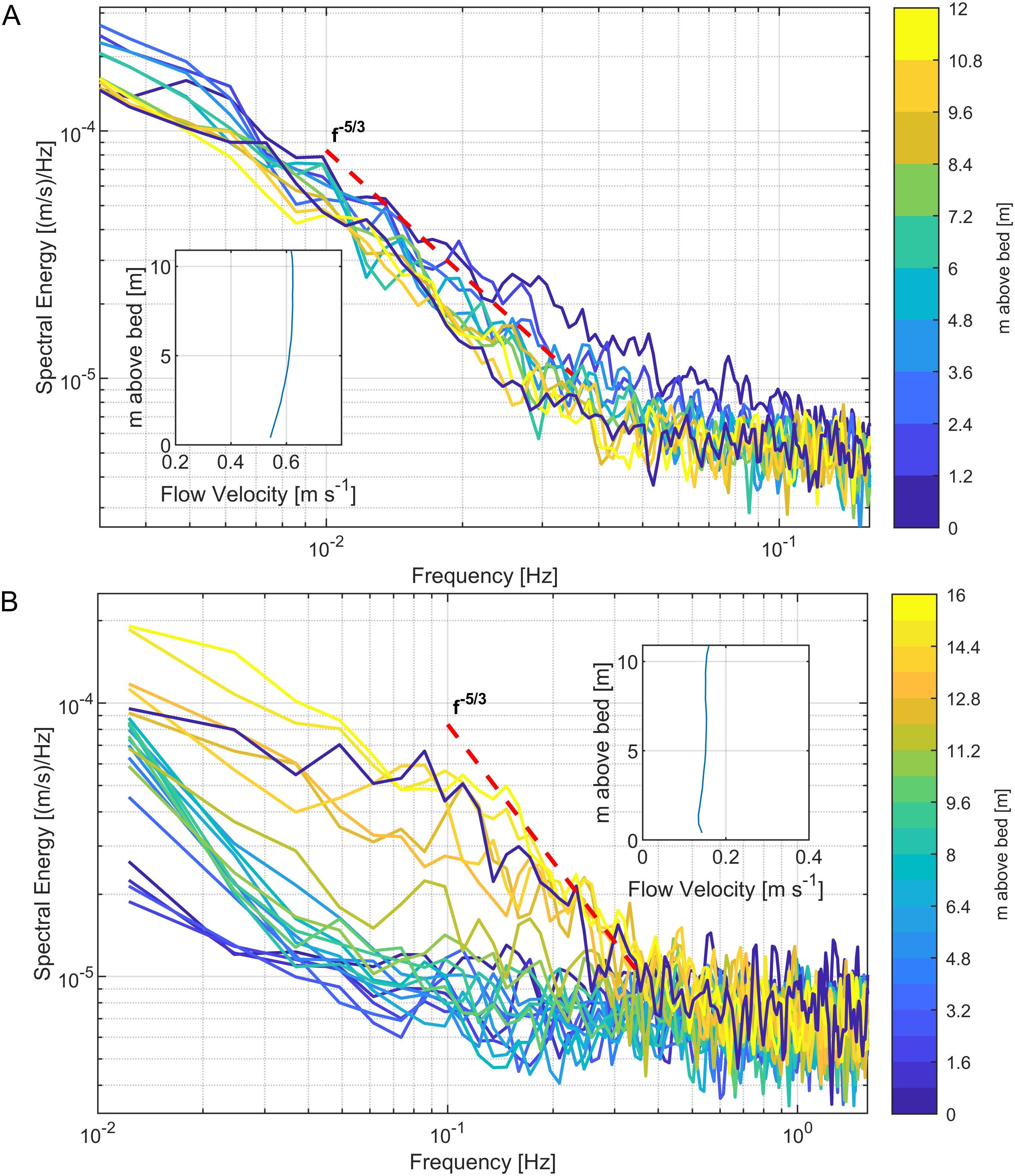
Figure 11. (A) Velocity power density spectrum from the deployment of the Nortek Signature during the maximum flood on the 11/15/2017 at study site I. The -5/3 slope as predicted by Kolmogorov (1941) is depicted as a red dashed line. (B) Velocity power density spectrum from the deployment of the Nortek Signature during the maximum flood on the 09/08/2017 at study site II.

The PSD plot also highlights the frequency range of turbulent motions studied here, spanning from 0.1 Hz to 0.5 Hz (periods of 10 to 2 seconds). This range falls within the inertial subrange of the Kolmogorov energy cascade and reflects low-frequency fluctuations typical of estuarine turbulence. These findings align with prior research. Suara et al. (2019) reported similar frequency ranges in tide-dominated estuaries, while Simpson et al. (2005) documented frequencies of 0.01–0.1 Hz in stratified estuaries. Stacey et al. (1999) observed buoyancy-induced turbulence below 0.1 Hz in partially stratified estuaries, and Orton et al. (2010) described tidal and atmospheric influences generating turbulence in the 0.1–0.3 Hz range near estuarine surfaces. This positioning within the inertial subrange highlights the study’s focus on intermediate-to-smaller turbulent motions, as opposed to the very smallest scales governed by viscosity or the largest scales driven by external forcing like tides or winds.

3.2.4.2 Study Site II

At Study Site II (Figure 11B), the PSD was far less uniform compared to Site I. The expected -5/3 slope of the inertial subrange was observed only in a few bins near the surface and the bed. In contrast, the majority of bins displayed no discernible slope. This lack of a consistent slope indicates variability in energy transfer across scales, likely driven by localized turbulence dynamics and disruptions caused by lateral and vertical flow interactions. These results underscore the more complex and less predictable nature of turbulence at Site II.

3.2.5 TKE, Eddy diffusivity; RS; ϵ

3.2.5.1 Study Site I

At study site II, high TKE was observed near the seabed during full running flows of both tidal cycles. Notably, during the first cycle, TKE extended into the upper and middle water columns (Figure 6A). This decoupling of TKE dynamics between the middle and lower water column suggests differing turbulence mechanisms between these regions, as highlighted by a line plot of TKE near the seabed and at mid-water column (Supplementary Figure 3). During spring tides, TKE spanned the entire water column, while during neap tides, it remained largely confined to the surface layer. This spatial and temporal pattern was mirrored in the depiction of Reynolds stresses (Figure 10A), further emphasizing the influence of tidal forcing on turbulence dynamics.

Panel B of Figure 6 shows the variation of eddy diffusivity (K) over time and height in the water column. Near the seabed (0.5 to 2 meters above the bed), eddy diffusivity was almost non-existent for most of the measurement period, except for a brief increase on 11/09. In the first half of the measurement period, K remained generally low throughout the water column, indicating minimal turbulence and mixing. However, during the ebb tide on 10/09, K began to increase and spread upward through the water column. In the second half of the period, eddy diffusivity increased significantly, becoming more dispersed across the entire water column, reflecting heightened turbulence and mixing variability driven by tidal processes.

The normalized PEA, plotted as a dashed black line in Figure 6A, quantifies the energy required to mix a stratified water column. PEA fluctuated in response to the semidiurnal tidal cycle, increasing during uniform ebb flow and decreasing during subsequent flood and ebb flows. This pattern was modulated by the spring-neap cycle, with PEA reaching higher baseline levels during neap tides. Notably, elevated TKE phases corresponded to reductions in PEA, signaling effective vertical mixing of the water column.

Figure 12A shows temperature variations across the water column, revealing thermoclines where warmer riverine water overlays cooler oceanic water. During spring tides, the lower tidal range allowed warmer water to extend further into the study area. Conversely, during neap tides, the entire water column became warmer. These temperature shifts influenced buoyancy dynamics, as reflected in N² in Figure 12B. During spring tides with elevated TKE, N² was positive throughout the water column, indicating stable stratification. However, during spring tides with smaller tidal ranges, N² varied more dynamically: positive at the bottom during flood and ebb tides, but negative at the surface during flood and throughout the water column during ebb. This shifting stratification suggests interactions between tidal flows, salinity, and temperature gradients. Notably, the evolution of N² aligned closely with PEA, where periods of negative N² corresponded to PEA buildup, and positive N² indicated enhanced vertical mixing.

Figure 12

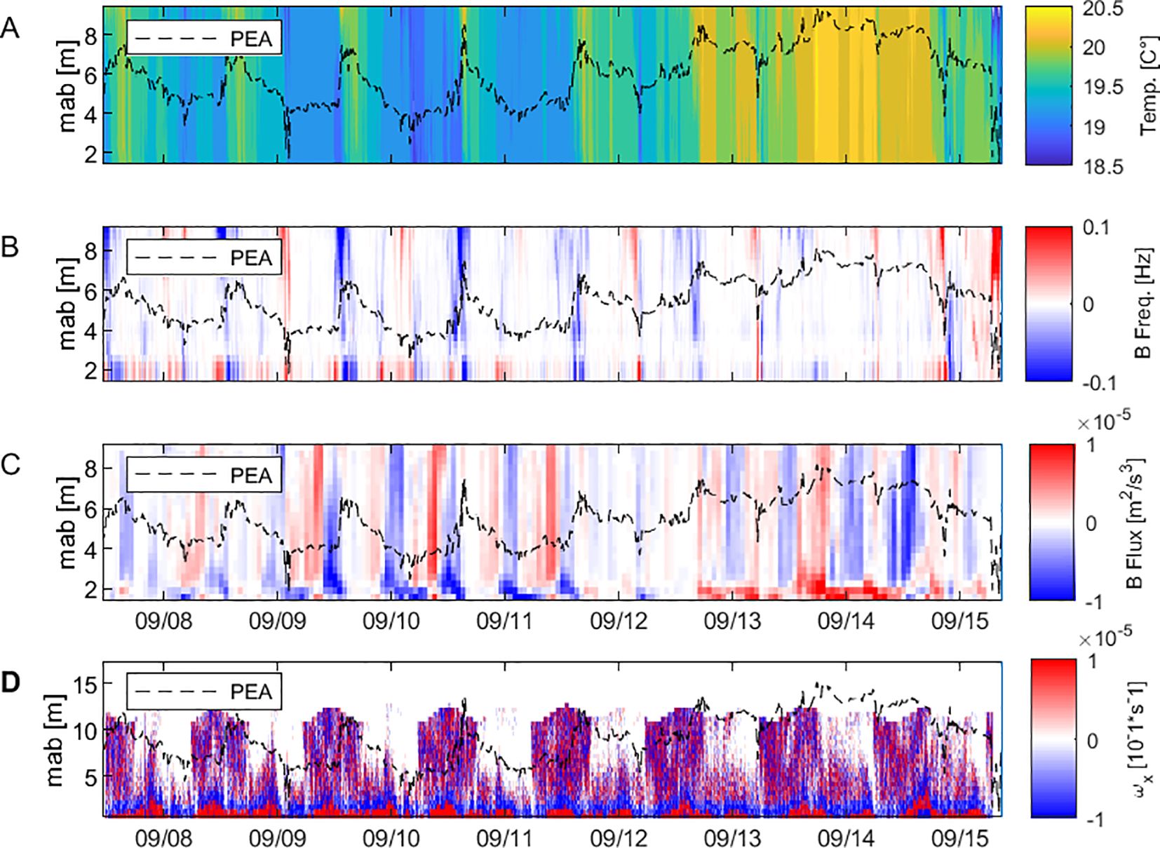
Figure 12. Depth-Time evolution of (A) Temperature, (B) N², (C) Buoyancy flux, (D) stream wise Vorticity.

Buoyancy flux (Figure 12C) varied significantly with the tidal cycle. During spring tide flood flows, positive buoyancy flux dominated the middle and upper water column, alternating with negative fluxes during high tide. Early ebb flow transitioned to negative flux, followed by neutral conditions. During neap tides, buoyancy flux patterns reversed: low tides showed alternating fluxes, while floods were marked by negative fluxes and ebbs by positive fluxes. Negative buoyancy flux during the first cycle’s ebb tide and near the surface during early ebb suggests downward buoyancy transfer, reinforcing stratification. In the second cycle, positive flux during flood tide may reflect buoyancy-driven upward motion. Variability in buoyancy flux during slack and ebb tides, coupled with strong negative flux at the bottom, highlights the complex interplay between tidal forcing, buoyancy, and stratification in modulating turbulence and mixing.

Streamwise vorticity (Figure 12D) exhibited a pronounced structure near the seabed, persisting through low water to high water phases, diminishing before re-developing in subsequent cycles. However, a blind spot near the seabed (due to the ADCP blanking distance) prevents observations within the bottom 0.5 meters. This structure likely persists across cycles, despite periods of apparent absence. Vorticity in the middle and upper water column displayed a regular pattern, intensifying during the first tidal cycle and weakening during the second.

Incorporating temperature variations (Figure 12A) clarifies the drivers of turbulent and buoyancy dynamics. For example, during the first flood tide, a drop in temperature (20 to 19.6 degrees Celsius) at slack tide corresponded with stable stratification, reflected by positive N² at the bottom. As the water warmed during the ebb tide, TKE developed in the upper and middle water column, promoting vertical mixing. This relationship recurred across cycles: cooler water during flood enhanced stratification and suppressed turbulence, while warmer water during ebb facilitated mixing, altering buoyancy flux patterns. For instance, the significant warming on 09/12/2017 coincided with a near-complete reduction in buoyancy flux.

Overall, the temperature variations across the tidal cycles provide a crucial context for interpreting the changes in TKE, N², and buoyancy flux. The thermal dynamics intertwined with tidal processes played a significant role in shaping the estuarine environment, influencing stratification, turbulence, and vertical mixing in a complex and cyclic manner.

3.2.6 Length and time scales

3.2.6.1 Study site I

Figure 13 shows the vertical variation in the mean values of the integral time and length scales across the water column at study site I. In panel A, the integral time scales exhibit fluctuating patterns with height. From 2 to 8 meters above the bed, mean values are approximately 5 seconds, indicating consistent turbulence within this region. Closer to the bed, between 0 and 2 meters, there is a slight rise to around 10 seconds, likely influenced by localized flow structures generated by bed friction.

Figure 13

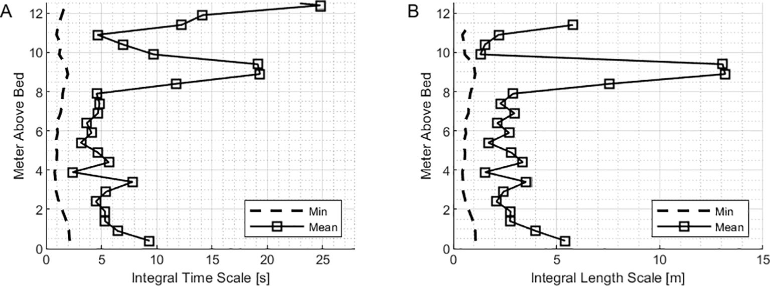
Figure 13. (A) Integral time and (B) length scales from study site I.

Above 8 meters, a notable increase in time scales is observed, rising to approximately 20 seconds between 8 and 10 meters. Interestingly, the time scale then decreases sharply to around 5 seconds at 11 meters, suggesting localized turbulence or transitional flow dynamics. Near the surface, beyond 11 meters, the time scales increase again, reaching approximately 25 seconds, reflecting the influence of surface-driven processes and larger-scale coherent flow structures.

In panel B, the integral length scales show a nuanced variation across the water column, similar to the trends observed for time scales. Near the bed, from 0 to 2 meters above the bed, mean values of length scales are relatively low, around 2–3 meters, reflecting small-scale turbulence dominated by bed friction. Between 2 and 8 meters above the bed, the length scales remain fairly consistent, averaging around 4 meters, indicating a relatively uniform but still turbulent flow regime in this mid-section of the water column. From 8 to 10 meters above the bed, there is a noticeable increase in the length scales, reaching approximately 8 meters, suggesting the emergence of larger, more coherent flow structures as the influence of bed turbulence decreases. However, at 11 meters, the length scales decrease back to around 5 meters, indicating a localized disruption or transitional flow dynamics, potentially due to interactions between turbulence and stratification. Near the surface, beyond 11 meters, the integral length scales increase again, peaking at approximately 10–12 meters. This reflects the dominance of surface-driven processes, such as wind shear and larger hydrodynamic structures, resulting in increased spatial coherence of velocity fluctuations. These trends highlight the transition from small-scale, turbulence-dominated flow near the bed to larger, more coherent structures near the surface, with an intermediate zone of fluctuating flow characteristics in the upper water column.

3.2.6.2 Study site II

At study site II the integral time scales exhibit a steady vertical structure across the water column (Figure 14), with significantly higher values compared to the middle reach of the river. Near the bed (0–2 meters above), the mean time scales start at approximately 50 seconds, indicating less intense turbulence compared to the middle reach. Between 2 and 8 meters, the time scales rise consistently, reaching approximately 250 seconds at 8 meters. Beyond 8 meters, the time scales increase further to around 300 seconds at 12 meters above the bed, reflecting the dominance of large, coherent flow structures near the surface, likely driven by tidal or wind-induced flows at the estuary mouth.

Figure 14

Figure 14. (A) Integral time and (B) length scales from study site II.

In panel B, the integral length scales also demonstrate a vertical increase, starting from approximately 5–10 meters near the bed (0–2 meters above). Between 2 and 8 meters, length scales increase steadily, reaching approximately 30 meters at 8 meters above the bed. In the upper water column, beyond 8 meters, length scales further rise, peaking at around 45 meters near the surface.

4 Discussion

At Study Sites I and II, the observed turbulence and mixing dynamics exhibit both alignment with established theories and deviations that highlight the complexities of estuarine processes. While some parameters, such as TKE and Reynolds stress, follow classical turbulence models, other relationships—such as those involving eddy diffusivity and buoyancy flux—reveal nuanced behaviors influenced by local stratification, lateral circulations, and thermal gradients.

At Site I, TKE is consistently generated near the seabed, closely correlating with shear velocity throughout the tidal cycle. This highlights bed friction as the dominant driver of turbulence, with limited contributions from lateral or stratification-driven mechanisms. During spring tides, TKE spans the entire water column, reflecting enhanced mixing, whereas during neap tides, turbulence remains confined near the bed. These trends align well with observations by Milne et al. (2017), which showed that spring tides amplify TKE distribution throughout the column, whereas neap tides restrict turbulence to the bottom layers.

RS profiles at Site I exhibit classical boundary-layer turbulence patterns, with peak values near the bed and rapid decreases with height. Maximum Reynolds stresses values occur during late tidal phases, such as ST+3h and ST+4h, before decreasing during slack tide. This predictable behavior aligns with studies by Stacey et al. (1999) and Greene et al. (2015), which documented similar reductions in Reynolds stresses with height due to reduced shear away from the bed.

In contrast, Site II exhibits more complex turbulence dynamics that diverge from classical theories. During spring tides, TKE extends vertically throughout the water column, reflecting strong mixing. However, during neap tides, turbulence is largely confined to the surface layers. TKE in the mid-column often decouples from near-bed turbulence during alternate tidal cycles, suggesting influences from lateral circulations and stratification. These observations align partially with findings by Collignon and Stacey (2013), which attributed near-surface TKE peaks during ebb tides to lateral density and velocity gradients. However, at Site II, TKE is present during both flood and ebb tides, with circulatory patterns playing a critical role. Horizontal flow reversals between flood and ebb phases generate significant shear and vorticity near the bed, driving localized TKE generation.

RS profiles at Site II are strongly phase-dependent. During spring tides, Reynolds stresses extend across the entire water column, while during neap tides, it diminishes rapidly with height due to stronger stratification. Near-bed Reynolds stresses peak dominate during ebb tides, but lateral circulatory patterns significantly influence Reynolds stresses in the upper column during flood phases. These findings align with Becherer et al. (2015), who observed Reynolds stresses variability driven by stratification and lateral flows in the German Wadden Sea.

Flow reversals at Site II, marked by high vorticity, low TKE, and gradient Richardson numbers exceeding 0.25, indicate highly stratified and stable conditions. These reversals, common in estuaries, intensify velocity gradients near the bed and stratified interfaces, generating vorticity. However, low TKE suggests that rotational energy does not cascade into turbulence, as strong stratification stabilizes the water column and suppresses turbulence, particularly in the mid- and upper layers.

The absence of TKE in the upper water column coincides with pronounced lateral velocity circulations extending throughout the full depth of the water column. This suggests that buoyancy flux and lateral advection, rather than shear-driven mechanisms, emerge as significant factors at Site II. Vorticity analysis supports this observation, showing regions of high TKE near the bed driven by shear, but decoupling in the mid-column and near-surface layers due to buoyancy flux and lateral dynamics.

4.1 Eddy diffusivity

Eddy diffusivity at Site II reveals distinct temporal and spatial variability, deviating from classical turbulence models. In the first half of the measurement period, eddy diffusivity is generally low throughout the water column, except for brief increases near the mid-column. However, during the ebb on 10/09, it begins to increase, spreading upward through the water column. In the second half of the record, eddy diffusivity increases over the entire water column, reflecting enhanced turbulence. Despite elevated TKE near the bed during certain periods, eddy diffusivity remains low, likely due to stable stratification indicated by positive N². This decoupling of eddy diffusivity from TKE contrasts with Osborn’s (1980) model, which assumes efficient conversion of TKE into mixing.

4.2 PEA, N² and flux

The normalized PEA and N² provide additional insights into stratification and mixing. Elevated TKE during spring tides corresponds to reductions in PEA, signaling effective mixing. Positive N² during these periods reflects stable stratification, which is overcome by high turbulence. During neap tides, N² varies dynamically, alternating between stability and instability, aligning with tidal phases.

Buoyancy flux complements these patterns, with positive values during spring tides indicating upward mixing and reduced stratification. Negative flux during neap tides, particularly near the bed during ebb phases, reinforces stratification, limiting vertical mixing. These findings align with MacCready and Geyer (2010), but the persistence of negative buoyancy flux near the seabed during ebb tides at Site II highlights unique site-specific dynamics, possibly driven by density gradients.

4.3 Integral time and lengths scales

Integral time and length scales also vary significantly between the two sites. At Site I, time scales near the bed range from 10 to 25 seconds, increasing steadily toward the surface, where larger-scale coherent structures dominate. Similarly, length scales near the bed range from 2–3 meters and increase to approximately 12 meters near the surface. These trends reflect a transition from small-scale, shear-driven turbulence at the bottom to surface-driven, larger-scale flows, consistent with findings by Milne et al. (2013) in tidal channels.

Site II, however, exhibits much larger time and length scales, particularly near the estuary mouth. Time scales near the surface exceed 300 seconds, while length scales reach up to 45 meters. Near the bed at Site II, time and length scales are shorter, reflecting the influence of bed shear, but these values increase significantly with height, influenced by lateral and stratification-driven processes.

4.4 Gradient Richardson number

Ri_g was calculated using ADCP and CTD data for two specific events. The first was on 09/07/2017 during high tide (Figures 15A–C), followed by a less turbulent ebb tide. The second occurred on 09/14/2017 during low water, succeeded by a less turbulent flood tide (Figures 15D–F).

Figure 15

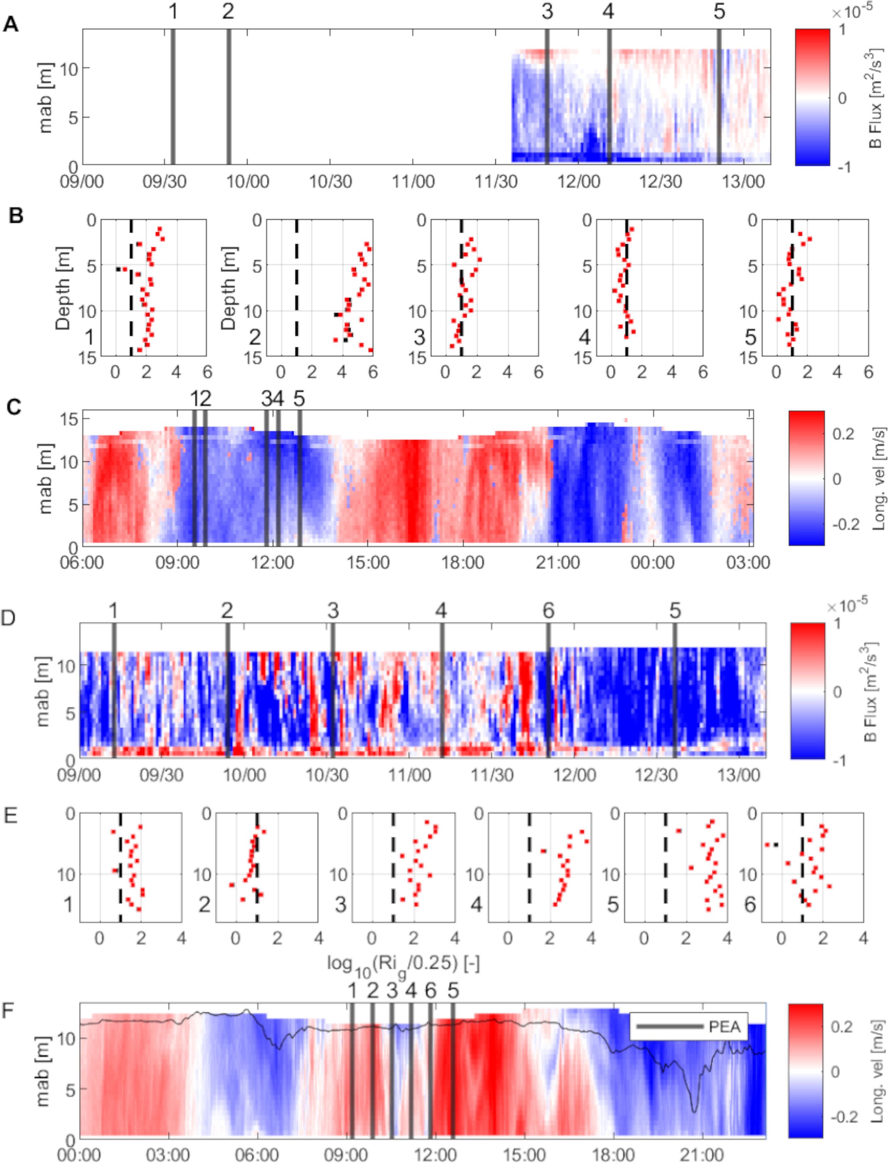
Figure 15. (A) Buoyancy Flux: Vertical lines mark the instances at which Conductivity-Temperature-Depth profiles were used for calculating the Gradient Richardson Number. (B) Gradient Richardson Number during high tide on 09/07/2017: A black vertical line delineates the threshold between conditions primarily influenced by mixing (Gradient Richardson Number< 1) and those influenced by stratification (Gradient Richardson Number > 1). Red dots represent profiles where density is calculated as a function of only salinity and temperature, while black dots indicate that sediment concentration was also included in the density calculation. (C) Longitudinal Velocity: Displayed concurrently with the other parameters for comparative purposes. (D) Buoyancy Flux: Included for further comparison. (E) Gradient Richardson Number during low tide on 09/14/2017, (F) Longitudinal Velocity: Provided for 09/14/2017, corresponding with panel (E).

For the high tide on 09/07/2017, Ri_g indicated a stratified water column. During the subsequent ebb tide, Ri_g fluctuated around the critical value of 0.25, signifying a balance between shear-driven mixing and stratification. The buoyancy flux (Figure 12A) became progressively more positive, indicating a mixing-dominated regime.

On 09/14/2017, during low water, Ri_g primarily remained above the critical 0.25 level, suggesting stratification (Figure 15E). The buoyancy flux was mostly negative, reinforcing this interpretation. A later profile exhibited a strong negative Ri_g, indicating an unstable, mixing-prone environment. The next three profiles were fully positive, denoting a stratification-dominant setting. The final profile during the flood tide returned to oscillating around the 0.25 threshold. The flow reversal period appeared to strongly stratify the water column. The buoyancy flux initially varied between positive and negative values in the first five profiles but turned predominantly negative in the last one, aligning with an unstable condition as indicated by Ri_g.

The use of Ri_g as a diagnostic tool for mixing and stratification is well established in estuarine studies. Peters and Bokhorst (2000) analyzed Ri_g in a partially mixed estuary using ADCP and CTD data, finding that stratification dominated when Ri_g exceeded 0.25. Their observations of increased shear during ebb tides align with findings at Site I, where ebb tide shear-driven mixing was evident.

Collignon and Stacey (2013) observed that Ri_g at the shoal–channel interface in San Francisco Bay dropped below 0.25 during late ebb tides, correlating with intensified turbulence. These dynamics were attributed to lateral density gradients, a mechanism also evident at Site II, where lateral flows influenced Rig and turbulence generation. However, Site II showed more persistent stratification during flood tides, a difference potentially due to estuarine morphology and tidal asymmetry.

Simpson et al. (2005) demonstrated the impact of tidal straining on Ri_g in a partially stratified estuary. They found that flood tides typically produced stratification (high Ri_g), while ebb tides favored mixing (low Ri_g). These patterns are consistent with those at Site I, where flood tides resulted in stratification and ebb tides induced shear-driven mixing. However, at Site II, localized turbulence during flood tides deviates from this pattern, suggesting site-specific influences such as geometry and lateral flows.

4.5 Measurement errors and lower limits of turbulence measurable

The measurements of the vertical velocities from the Nortek Signature were crucial for the calculation of turbulence parameters and the hypotheses made on sediment transport. Additionally, in order to validate that the vertical velocities measured by the Nortek Signature were not simply erroneous, data from the RDI ADCP was used for validation. However, the resolution, instrument noise, and missing vertical beam of the RDI ADCP were limiting factors compared to the Nortek Signature. Nonetheless, both datasets show agreement when the magnitude of vertical velocities and therefore the signal was strongest (see Supplementary Figure 2). Furthermore, the moving average filter (10-minute window) used on the vertical velocities reduced random errors. The limit for the smallest Reynolds stresses can be assessed with an approach by Williams and Simpson (2004):

$\begin{array}{ll}{\sigma }_R^2\begin{array}{c}=\frac{\gamma {\left({\sigma }_n^2-\langle b_i^2\rangle \right)}^2}{Msi{n}^{2}2\theta }\end{array}& (20)\end{array}$

where γ: factor for covariance between individual velocity values; M: number of measurements included for the estimate; σ_n²: variance due to noise level from instrument; b_i^²: variance due to velocity fluctuations.

Assuming that during low flow, the velocity approaches zero, γ = 1 (variance due to noise alone, therefore no correlation), the instrument noise level being 4.6 cm s^-1, and N = 480, using Equation 16 we calculated a minimum of noise and therefore a minimum value for measurable stress of 1.29 × 10-4 m² s^-2. The scale of Reynolds stresses measured was an order of magnitude larger than the calculated minimal value, suggesting that the measurement and estimation principles are robust.

5 Conclusion

We examined the disparities between consecutive tidal cycles in a setting influenced by a mixed semidiurnal tide. Tidal cycles with lower turbulence were generally characterized by a dynamic equilibrium between shear-induced mixing and stratification, as quantified by Ri_g. These cycles exhibited pronounced streamwise vorticity throughout the water column. Conversely, in cycles with heightened turbulence, this vorticity diminished while TKE in the upper water column increased. This was accompanied by prominent lateral circulations.

In summary, our research enhances the existing body of knowledge on turbulence dynamics within estuarine systems. By comparing Sites I and II, we observed significant variability in turbulence drivers. At Site I, bed friction was the dominant driver, aligning well with classical theories, while Site II exhibited more complex dynamics influenced by lateral circulations, stratification, and phase-dependent interactions. The relationship between TKE and eddy diffusivity deviated from classical models in stratified conditions, underscoring the need to incorporate lateral and buoyancy-driven dynamics into existing frameworks.

Data availability statement

The raw data supporting the conclusions of this article will be made available by the authors, without undue reservation.

Author contributions

JT: Writing – original draft, Writing – review & editing. RC: Writing – review & editing. JV: Writing – review & editing. AG: Writing – review & editing. TS: Writing – review & editing.

Funding

The author(s) declare that no financial support was received for the research, authorship, and/or publication of this article.

Acknowledgments

We would like to thank the members of the Aquatic Systems research group of the University of Queensland for the fruitful technical discussions and hands-on support in the field. This research was made possible through the logistical support of the Port of Brisbane.

Conflict of interest

The authors declare that the research was conducted in the absence of any commercial or financial relationships that could be construed as a potential conflict of interest.

The author(s) declared that they were an editorial board member of Frontiers, at the time of submission. This had no impact on the peer review process and the final decision.

Publisher’s note

All claims expressed in this article are solely those of the authors and do not necessarily represent those of their affiliated organizations, or those of the publisher, the editors and the reviewers. Any product that may be evaluated in this article, or claim that may be made by its manufacturer, is not guaranteed or endorsed by the publisher.

Supplementary material

The Supplementary Material for this article can be found online at: https://www.frontiersin.org/articles/10.3389/fmars.2025.1447316/full#supplementary-material

Supplementary Figure 1 | Relation between temperature and density (computed from Salinity and Temperature) from the CTD profiles.

Supplementary Figure 2 | Vertical velocities from the RDI ADCP. Positive =upwards, negative = downwards.

Supplementary Figure 3 | TKE in bin 1 (near the bed) and bin 15 (middle of the water column).

References

Bakhoday-Paskyabi M., Fer I., Reuder J. (2018). Current and turbulence measurements at the FINO1 offshore wind energy site: analysis using 5-beam ADCPs. Ocean Dynamics 68, 109–130. doi: 10.1007/s10236-017-1109-5

Crossref Full Text | Google Scholar

Becherer J., Stacey M. T., Umlauf L., Burchard H. (2015). Lateral circulation generates flood tide stratification and estuarine exchange flow in a curved tidal inlet. J. Phys. Oceanography 45, 638–656. doi: 10.1175/JPO-D-14-0001.1

Crossref Full Text | Google Scholar

Beecroft R., Grinham A., Albert S., Perez L., Cossu R. (2019). Suspended sediment transport in context of dredge placement operations in moreton bay, Australia. J. Waterway Port Coastal Ocean Eng. 145, 05019001. doi: 10.1061/(ASCE)WW.1943-5460.0000503

Crossref Full Text | Google Scholar

Bolaños R., Brown J. M., Souza A. J. (2014). Wave–current interactions in a tide dominated estuary. Continental Shelf Res. 87, 109–123. doi: 10.1016/j.csr.2014.05.009

Crossref Full Text | Google Scholar

Boyd R., Dalrymple R., Zaitlin B. A. (1992). Classification of clastic coastal depositional environments. Sedimentary Geology 80, 139–150. doi: 10.1016/0037-0738(92)90037-R

Crossref Full Text | Google Scholar

Burchard H. (2002). Applied Turbulence Modelling in Marine Waters (Berlin, Heidelberg: Springer-Verlag). doi: 10.1007/3-540-45419-5

Crossref Full Text | Google Scholar

Burchard H., Baumert H. (1998). The formation of estuarine turbidity maxima due to density effects in the salt wedge. A hydrodynamic process study. J. Phys. Oceanogr. 28, 309–321. doi: 10.1175/1520-0485(1998)028<0309:TFOETM>2.0.CO;2

Crossref Full Text | Google Scholar

Burchard H., Hofmeister R. (2008). A dynamic equation for the potential energy anomaly for analysing mixing and stratification in estuaries and coastal seas. Estuarine Coast. Shelf Sci. 77, 679–687. doi: 10.1016/j.ecss.2007.10.025

Crossref Full Text | Google Scholar

Chant R. J., Geyer W. R., Houghton R., Hunter E., Lerczak J. (2007). Estuarine boundary layer mixing processes: insights from dye experiments. J. Phys. Oceanogr. 37, 1859–1877. doi: 10.1175/JPO3088.1

Crossref Full Text | Google Scholar

Codiga D. L. (2011). Unified Tidal Analysis and Prediction Using the UTide Matlab Functions (Narragansett, RI, USA: Graduate School of Oceanography, University of Rhode Island). doi: 10.13140/RG.2.1.3761.2008

Crossref Full Text | Google Scholar

Collignon A. G., Stacey M. T. (2013). Turbulence dynamics at the shoal–channel interface in a partially stratified estuary. J. Phys. Oceanography 43, 970–989. doi: 10.1175/JPO-D-12-0115.1

Crossref Full Text | Google Scholar

Davie P., Stock E., Low Choy D. C. (1990). The Brisbane River: A Source-book for the Future. Australian Littoral Society, Brisbane, Australia.

Google Scholar

Dewey R., Stringer S. (2007). Reynolds stresses and turbulent kinetic energy estimates from various ADCP beam configurations: theory. doi: 10.13140/RG.2.1.1042.8002. Unpublished.

Crossref Full Text | Google Scholar

Geyer W. R., MacCready P. (2014). The estuarine circulation. Annu. Rev. Fluid Mechanics 46, 175–197. doi: 10.1146/annurev-fluid-010313-141302

Crossref Full Text | Google Scholar

Greene A. D., Hendricks P. J., Gregg M. C. (2015). Using an ADCP to estimate turbulent kinetic energy dissipation rate in sheltered coastal waters. J. Atmos. Oceanic Technol. 32, 318–333. doi: 10.1175/JTECH-D-13-00207.1

Crossref Full Text | Google Scholar

Greenwood C., Vogler A., Venugopal V. (2019). On the variation of turbulence in a high-velocity tidal channel. Energies 12, 672. doi: 10.3390/en12040672

Crossref Full Text | Google Scholar

Hansen D. V., Rattray M. (1966). NEW DIMENSIONS IN ESTUARY CLASSIFICATION1. Limnology Oceanography 11, 319–326. doi: 10.4319/lo.1966.11.3.0319

Crossref Full Text | Google Scholar

Hughes H., Hubble (1998). Dynamics of the turbidity maximum zone in a micro-tidal estuary: Hawkesbury River, Australia. Sedimentology 45, 397–410. doi: 10.1046/j.1365-3091.1998.0159f.x

Crossref Full Text | Google Scholar

Huguenard K. D., Valle-Levinson A., Li M., Chant R. J., Souza A. J. (2015). Linkage between lateral circulation and near-surface vertical mixing in a coastal plain estuary. J. Geophysical Research-Oceans 120, 4048–4067. doi: 10.1002/2014JC010679

Crossref Full Text | Google Scholar

Imamura J., Takagi K., Nagaya S. (2018). Engineering analysis of turbulent flow measurements near Kuchinoshima Island. J. Mar. Sci. Technol. 33, 1. doi: 10.1007/s00773-018-0573-z

Crossref Full Text | Google Scholar

Islam R. (2024). Despiking Acoustic Doppler Velocimeter (ADV) Data. Available online at: https://de.mathworks.com/matlabcentral/fileexchange/39767-despiking-acoustic-doppler-velocimeter-adv-data (Accessed December 18, 2024).

Google Scholar

Islam M. R., Zhu D. Z. (2013). Kernel density–based algorithm for despiking ADV data. J. Hydraulic Eng. 139, 785–793. doi: 10.1061/(ASCE)HY.1943-7900.0000734

Crossref Full Text | Google Scholar

Jay D. A., Smith J. D. (1990). Circulation, density distribution and neap-spring transitions in the Columbia River Estuary. Prog. Oceanography 25, 81–112. doi: 10.1016/0079-6611(90)90004-L

Crossref Full Text | Google Scholar

Kundu P. K., Cohen I. M., Dowling D. R., Tryggvason G. (2016). Fluid mechanics, Sixth Edition. Amsterdam Boston Heidelberg London: Elsevier, Academic Press.

Google Scholar

Liu H., Wu J. (2015). Estimation of bed shear stresses in the pearl river estuary. China Ocean Eng. 29, 133–142. doi: 10.1007/s13344-015-0010-6

Crossref Full Text | Google Scholar

Lockington J. R., Albert S., Fisher P. L., Gibbes B. R., Maxwell P. S., Grinham A. R. (2017). Dramatic increase in mud distribution across a large sub-tropical embayment, Moreton Bay, Australia. Mar. pollut. Bull. 116, 491–497. doi: 10.1016/j.marpolbul.2016.12.029

PubMed Abstract | Crossref Full Text | Google Scholar

Lohrmann A., Hackett B., Roed L. P. (1990). High resolution measurements of turbulence, velocity and stress using a pulse-to-pulse coherent sonar. J. Atmos. Ocean. Technol. 7, 19–37. doi: 10.1175/1520-0426(1990)007<0019:hrmotv>2.0.co;2

Crossref Full Text | Google Scholar

MacCready P., Geyer W. R. (2010). Advances in estuarine physics. Ann. Rev. Mar. Sci. 2, 35–58. doi: 10.1146/annurev-marine-120308-081015

PubMed Abstract | Crossref Full Text | Google Scholar

Manning A. J., Schoellhamer D. H. (2013). Factors controlling floc settling velocity along a longitudinal estuarine transect. Mar. Geology 345, 266–280. doi: 10.1016/j.margeo.2013.06.018

Crossref Full Text | Google Scholar

Milne I. A., Sharma R. N., Flay R. G. J. (2017). The structure of turbulence in a rapid tidal flow. Proc. Math Phys. Eng. Sci. 473, 20170295. doi: 10.1098/rspa.2017.0295

PubMed Abstract | Crossref Full Text | Google Scholar

Marées C. A. (1938). Service Hydrographique de la Marine.

Google Scholar

McDougall T. J., Barker P. M. (2011). Getting started with TEOS-10 and the Gibbs Seawater (GSW) Oceanographic Toolbox, 28pp., SCOR/IAPSO WG127, ISBN 978-0-646-55621-5.

Google Scholar

Milne I. A., Sharma R. N., Flay R. G. J., Bickerton S. (2013). Characteristics of the turbulence in the flow at a tidal stream power site. Philos. Trans. A Math Phys. Eng. Sci. 371, 20120196. doi: 10.1098/rsta.2012.0196

PubMed Abstract | Crossref Full Text | Google Scholar

Nielsen J. E. C. (2019). Reducing the Turbidity of the Brisbane River Estuary, Australia. The University of Queensland. doi: 10.14264/uql.2019.686

Crossref Full Text | Google Scholar

Olabarrieta M., Warner J. C., Kumar N. (2011). Wave-current interaction in willapa bay. J. Geophys. Res. 116. doi: 10.1029/2011JC007387

Crossref Full Text | Google Scholar

Orton P. M., Zappa C. J., McGillis W. R. (2010). Tidal and atmospheric influences on near-surface turbulence in an estuary. J. Geophysical Research: Oceans 115. doi: 10.1029/2010JC006312

Crossref Full Text | Google Scholar

Osborn T. R. (1980). Estimates of the Local Rate of Vertical Diffusion from Dissipation Measurements. Available online at: https://journals.ametsoc.org/view/journals/phoc/10/1/1520-0485_1980_010_0083_eotlro_2_0_co_2.xml (Accessed December 19, 2024).

Google Scholar

Peters H. (1997). Observations of stratified turbulent mixing in an estuary: neap-to-spring variations during high river flow. Estuarine Coast. Shelf Sci. 45, 69–88. doi: 10.1006/ecss.1996.0180

Crossref Full Text | Google Scholar

Peters H., Bokhorst R. (2000). Microstructure Observations of Turbulent Mixing in a Partially Mixed Estuary. Part I: Dissipation Rate. Available online at: https://journals.ametsoc.org/view/journals/phoc/30/6/1520-0485_2000_030_1232_mootmi_2.0.co_2.xml (Accessed December 19, 2024).

Google Scholar

Pritchard D. W. (1954). A study of the salt balance in a coastal plain estuary. J. Mar. Res. 13, 133–144.

Google Scholar

Ralston D. K., Geyer W. R., Lerczak J. A., Scully M. (2010). Turbulent mixing in a strongly forced salt wedge estuary. J. Geophysical Research: Oceans 115. doi: 10.1029/2009JC006061

Crossref Full Text | Google Scholar

Richardson D., Devlin T., Ettema S. (2017). Port of Brisbane Monitoring Program – Assessment of Sediment from 2017 Maintenance Dredging Activities. Available online at: https://www.portbris.com.au/getmedia/79cbd29a-3eeb-4c19-922a-e9f72a6bdb39/2017-10-12-R-B20259-028-02-Dredge-Turbidity-FINAL_1.pdf (Accessed June 10, 2024).

Google Scholar

Rippeth T. P., Fisher N. R., Simpson J. H. (2001). The cycle of turbulent dissipation in the presence of tidal straining. J. Phys. Oceanography 31, 2458–2471. doi: 10.1175/1520-0485(2001)031<2458:TCOTDI>2.0.CO;2

Crossref Full Text | Google Scholar

Ross L., Huguenard K., Sottolichio A. (2019). Intratidal and fortnightly variability of vertical mixing in a macrotidal estuary: the gironde. J. Geophysical Research-Oceans 124, 2641–2659. doi: 10.1029/2018JC014456

Crossref Full Text | Google Scholar

Rusello P. J., Cowen E. A. (2011). “Turbulent dissipation estimates from pulse coherent doppler instruments,” in IEEE/OES 10th current, waves and turbulence measurements (CWTM). Eds. Monterey C. A., Rizoli White J. (IEEE, Piscataway, NJ), 167–172. doi: 10.1109/CWTM.2011.5759546

Crossref Full Text | Google Scholar

Scully M. E., Geyer W. R., Lerczak J. A. (2009). The influence of lateral advection on the residual estuarine circulation: A numerical modeling study of the hudson river estuary. J. Phys. Oceanogr. 39, 107–124. doi: 10.1175/2008JPO3952.1

Crossref Full Text | Google Scholar

Sentchev A., Thiébaut M., Guillou S. (2021). “Turbulence characterization at tidal-stream energy site in Alderney Race,” in Developments in renewable energies offshore: Proceedings of the 4th International Conference on Renewable Energies Offshore (RENEW 2020). Ed. Soares C. G. (CRCPress/Balkema, Boca Raton), 616–623.

Google Scholar

Simpson J., Bos W., Schirmer F., Souza A., Rippeth T., Jones S., et al. (1993). Periodic stratification in the rhine ROFI in the north-sea. Oceanologica Acta 16, 23–32.

Google Scholar

Simpson J. H., Williams E., Brasseur L. H., Brubaker J. M. (2005). The impact of tidal straining on the cycle of turbulence in a partially stratified estuary. Continental Shelf Res. 25, 51–64. doi: 10.1016/j.csr.2004.08.003

Crossref Full Text | Google Scholar

Soulsby R. L. (1980). Selecting record length and digitization rate for near-bed turbulence measurements. J. Phys. Oceanogr. 10, 208–219. doi: 10.1175/1520-0485(1980)010<0208:SRLADR>2.0.CO;2

Crossref Full Text | Google Scholar

Stacey M. T., Monismith S. G., Burau J. R. (1999). Observations of turbulence in a partially stratified estuary. J. Phys. Oceanogr. 29, 1950–1970. doi: 10.1175/1520-0485(1999)029<1950:OOTIAP>2.0.CO;2

Crossref Full Text | Google Scholar

Stacey M. T., Ralston D. K. (2005). The scaling and structure of the estuarine bottom boundary layer. J. Phys. Oceanography 35, 55–71. doi: 10.1175/JPO-2672.1

Crossref Full Text | Google Scholar

Suara K. A., Brown R., Chanson H. (2019). Characteristics of flow fluctuations in a tide-dominated estuary: Application of triple decomposition technique. Estuarine Coast. Shelf Sci. 218, 119–130. doi: 10.1016/j.ecss.2018.12.006

Crossref Full Text | Google Scholar

Taebel Z., McAllister M. L., Scotti A., Onorato M., van den Bremer T. S. (2024). Laboratory study of wave turbulence under isotropic forcing. Phys. Rev. Fluids 9, 94803. doi: 10.1103/PhysRevFluids.9.094803

Crossref Full Text | Google Scholar

Taylor G. I. (1935). Statistical theory of turbulence. Proc. R. Soc. London. Ser. A Math. Phys. Sci. 151, 421–444.

Google Scholar

Toffolon M., Vignoli G., Tubino M. (2006). Relevant parameters and finite amplitude effects in estuarine hydrodynamics. J. Geophysical Research: Oceans 111. doi: 10.1029/2005JC003104

Crossref Full Text | Google Scholar

Trevethan M., Chanson H., Brown R. (2008). Turbulent measurements in a small subtropical estuary with semidiurnal tides. J. Hydraul. Eng. 134, 1665–1670. doi: 10.1061/(ASCE)0733-9429(2008)134:11(1665

Crossref Full Text | Google Scholar

Waltham N. J., Connolly R. M. (2011). Global extent and distribution of artificial, residential waterways in estuaries. Estuarine Coast. Shelf Sci. 94, 192–197. doi: 10.1016/j.ecss.2011.06.003

Crossref Full Text | Google Scholar

Wilber D. H., Clarke D. G. (2001). Biological effects of suspended sediments: A review of suspended sediment impacts on fish and shellfish with relation to dredging activities in estuaries. North Am. J. Fisheries Manage. 21, 855–875. doi: 10.1577/1548-8675(2001)021<0855:BEOSSA>2.0.CO;2

Crossref Full Text | Google Scholar

Wiles P. J., Rippeth T. P., Simpson J. H., Hendricks P. J. (2006). A novel technique for measuring the rate of turbulent dissipation in the marine environment. Geophys. Res. Lett. 33, 422. doi: 10.1029/2006GL027050

Crossref Full Text | Google Scholar

Williams E., Simpson J. H. (2004). Uncertainties in estimates of reynolds stress and TKE production rate using the ADCP variance method. J. Atmos. Oceanic Technol. 21, 347–357. doi: 10.1175/1520-0426(2004)021<0347:UIEORS>2.0.CO;2

Crossref Full Text | Google Scholar

Zippel S. F., Farrar J. T., Zappa C. J., Miller U., St. Laurent L., Ijichi T., et al. (2021). Moored turbulence measurements using pulse-coherent doppler sonar. J. Atmos. Oceanic Technol. 1621–1639. doi: 10.1175/JTECH-D-21-0005.1

Crossref Full Text | Google Scholar