Fine-scale hydrodynamics around St. John, U.S. Virgin Islands. Part I: spatial and temporal heterogeneity in the coastal environment

Physical conditions in coastal ecosystems can vary dramatically in space and time, influencing marine habitats and species distribution. However, such physical variability is often overlooked in ecological research, particularly in coral reef research and conservation. This study aims to quantify fine-scale variability in the physical conditions of a coastal environment to provide critical context for coastal ecosystem conservation and coral reef restoration. By developing and analyzing a 50 m-resolution hydrodynamic model, we characterize the physical oceanographic environment around the tropical island of St. John, U.S. Virgin Islands. Model simulations reveal that tides, winds, and the Amazon and Orinoco River plumes, interacting with the complex coastline and seafloor topography, create significant spatial and temporal variability in the coastal environment. Differences in tidal characteristics between the north and south shores generate strong oscillatory tidal flows in the channels surrounding St. John. The mean flow around the island is predominantly westward, driven by prevailing easterly winds. Water temperature and salinity exhibit variability over relatively small length scales, with characteristic alongshore length scales of 3–10 km, depending on the season. Hydrodynamic conditions also vary across multiple time scales. Strong tidal flows interacting with headland geometry produce transient eddies with strong convergent/divergent flows and variability on the scale of hours. Synoptic-scale flow variations are driven by weather events, while seasonal variations are strongly influenced by the Amazon and Orinoco River plumes. During summer and fall, these river plumes freshen the waters on the south shore of St. John, creating significant salinity differences between the north and south shores. These fine-scale physical variabilities can exert a strong influence on the coastal ecosystem and should be considered in the management of coastal resources. By providing a detailed understanding of the physical environment, this study supports efforts to conserve and restore coastal ecosystems, particularly coral reefs, in the face of dynamic and complex oceanographic conditions.

1 Introduction

Tropical island ecosystems are hubs of ocean biodiversity. Coral reefs, along with their integrated mangrove and seagrass communities, support an estimated 25% of all marine life and provide billions of dollars in ecosystem services, including shoreline protection and food resources (Knowlton et al., 2010; Guannel et al., 2016; Reguero et al., 2021). However, these ecosystems are increasingly threatened by climate change and other changes of the ocean physical environment. Such changes can drive various forms of ecological stress, including coral bleaching and seagrass bed eutrophication (e.g., Harborne et al., 2017; El-Hacen et al., 2019). Despite their importance, the fine-scale environmental variability of tropical coastal habitats remains poorly understood.

Coastal dynamics in the Caribbean region are influenced by multiple factors, particularly tides and winds. Tides in the northeastern Caribbean Sea are predominantly diurnal (Kjerfve, 1981), whereas the Atlantic side of Lesser Antilles experiences mostly semidiurnal tides (Pringle et al., 2019). At the boundary between the Atlantic Ocean and the Caribbean Sea, strong tidal currents, exceeding 2 m s^-1, occur in the channels of the island chain, including those between Puerto Rico and the Virgin Islands (Gonzalez-Lopez, 2015). The region is also subject to prevailing easterly winds (Figure 1B), which drive a dominant westward flow on the shelf (Centurioni and Niiler, 2003; Gonzalez-Lopez, 2015). Episodic hurricanes significantly alter local ocean circulation (Joyce et al., 2019). Additionally, plumes from the Amazon and Orinoco Rivers reach the eastern Caribbean Sea, contributing to seasonal variations in surface salinity (Froelich et al., 1978). When these plumes extend northwestward across the basin, they can affect regional flows in the Caribbean Sea (Chérubin and Richardson, 2007).

Figure 1

Figure 1. Maps of (A) the model domain and shelf bathymetry and (C) the St. John study region, and (B) wind rose of 2016–2022 ERA5 hourly wind, with 5° directional beam. Thick black lines in (A, C) mark coastlines. In (A), the blue color shows shelf bathymetry between 3 and 50 m; Gray dashed and solid lines are 100 and 300 m isobath contours, respectively; The red diamond marks the location of NOAA Buoy 41052; The blue rectangle marks the interior edge of the model boundary relaxation zone; The red rectangle marks area of (C). In (C), thin gray contours denote the 16 m isobath contour; red dashed line denote a smoothed 16 m isobath contour used in Figure 8; blue numbers 1–5 denote five selected coral reef sites. Orange lines denote the across-shelf transects of temperature and salinity shown in Figure 9; the magenta rectangle marks the Ram Head headland region with prominent eddies as shown in Figure 13.

Located at the border between the northeast Caribbean Sea and the Atlantic Ocean (Figure 1A), the island of St. John, U.S. Virgin Islands (US-VI), offers a compelling setting to explore the interplay of physical influences on coastal tropical habitats. The island is encircled by a shallow shelf—10 to 40 km wide and less than 50 m deep—that transitions abruptly to depths exceeding 1000 m over a narrow continental slope. St. John is separated from St. Thomas to the west by a 3 km wide channel and from the British Virgin Islands to the east and northeast by a 1 km wide channel, both approximately 30 m deep. Its shoreline is highly complex, featuring more than a dozen coastal bays of various shapes and sizes (Figure 1C). The shelf water surrounding St. John originate from multiple sources, including Caribbean surface water, subtropical underwater, and Sargasso Sea Water (Seijo-Ellis et al., 2019). Moreover, Seijo-Ellis et al. (2023) demonstrated that low-salinity near-surface waters in the Virgin Islands coastal region can originate from the Amazon and Orinoco Rivers. Consequently, the hydrodynamic environment around St. John is inherently complex, likely exhibiting fine‐scale temporal and spatial variability that has yet to be systematically quantified.

Much of the seafloor surrounding St. John is covered by coral reefs, seagrass meadows, and mangrove forests. About two-thirds of the island is designated as a U.S. National Park, offering broad protection for local flora and fauna while limiting some human impacts. However, despite this protection, the St. John coastal ecosystem is undergoing significant changes driven by both natural processes and large-scale anthropogenic influences.

One of the most pressing concerns is the rapid degradation of coral reefs (e.g., Rogers and Miller, 2006; Edmunds, 2013; Becket et al., 2020; Levitan et al., 2023; Godard et al., 2024). Coral diseases, such as Stony Coral Tissue Loss Disease in the U.S. Virgin Islands, have decimated local reefs, including those around St. John (Brandt et al., 2021; Cetina-Heredia and Allende-Arandía, 2023). However, disease spread has at times been patchy, with areas like Coral Bay temporarily serving as refuges (Brandt et al., 2021). Given these ongoing changes, it is crucial to quantify the variability of the physical environment to better understand and protect this fragile coastal ecosystem.

Physical conditions influence coastal ecosystems by affecting coral growth, species metabolism, nutrient delivery, larval dispersal, and contaminant transport (Lugo-Fernández et al., 2004; Sponaugle et al., 2005). A comprehensive understanding of the hydrodynamic environment—particularly its fine‐scale spatial and temporal variations—is crucial for unraveling the complex biological and chemical processes within these sensitive coastal ecosystems (Monismith, 2007). Quantifying hydrodynamic variability, including the flushing time of water in coastal bays, can also help inform conservation and restoration efforts. Identifying sites less impacted by storm forcing and climate warming, as well as regions of larvae aggregation and improved water quality, can help enhance coral reef resilience in the region (Viehman et al., 2023).

This 2-part study aims to provide a description of the fine-scale variability of the physical environment in the coastal region around St. John for researchers studying and policy makers managing the coastal ecosystem. The findings will offer essential context for interpreting biological and biogeochemical data collected in the region and guide future coastal resource conservation efforts (Kaplan et al., 2015; Brandt et al., 2021; Becker et al., 2024). Due to sparsity of observational data in the region, these can only be achieved through high-resolution numerical modeling. In this Part I paper, we use a high-resolution 3-dimensional (3D) numerical ocean model to assess the impacts of major forcings on coastal conditions around the island. The Part II paper (Jia et al., 2025) examines the exchange processes between the bays around St. John and the broader coastal region. Surface waves are not included in this model and will be included in future work. This paper is structured as follows: Section 2 describes the model configuration, observational data, and analysis methods. Section 3 presents the modeled hydrodynamic variability, including tides, currents, temperature, and salinity. Section 4 discusses the implications and caveats of the findings, and Section 5 provides a summary of the results.

2 Methods

2.1 Hydrodynamic model

The hydrostatic Regional Ocean Modeling System (ROMS; version revision 1219; Shchepetkin and McWilliams, 2005; Haidvogel et al., 2008) is used to simulate fine-scale hydrodynamics in the St. John area. ROMS is a free-surface, terrain-following, primitive-equations ocean model and has been used to simulate nearshore environments, including coral reef atolls with complex bathymetry (e.g., Rogers et al., 2017). The ROMS-based St. John model is configured with the following characteristics.

1) Model domain and grid resolution. The domain extends longitudinally from 65.25°W to 64°W and latitudinally from 17.9°N to 18.9°N (Figure 1A), encompassing St. John, St. Thomas, the British Virgin Islands, and the adjacent shelf. The model has open boundaries on all four sides. Around St. John, the horizontal grid resolution is 50 m, significantly finer than the 250–500 m resolution recommended for coral reef studies (Saint-Amand et al., 2023). The model includes 25 terrain-following vertical layers.

2) Bathymetry. A high-resolution model bathymetry for the shallow shelf was constructed by merging a 1-arcsecond US-VI Coastal Digital Elevation Model (NOAA National Geophysical Data Center, 2010), a 3-arcsecond Puerto Rico U.S. Coastal Relief Model (NOAA National Geophysical Data Center, 2005), and the NOAA ETOP01 1-arcminute global relief model (Amante and Eakins, 2009). The minimum depth is 5 m. Because the deep ocean part of the model is relaxed to the unsteady 3D fields provided by a global ocean model, the maximum depth of the St. John model is limited to 300 m to ensure high resolution in the upper water column. Rogers et al. (2017) demonstrated that this treatment does not affect solutions in shallow coastal regions, which are the primary focus of this study. However, due to the depth limitation, the model is not suitable for studying the influence of deep ocean processes, such as internal tides, on the shelf.

3) Model parameterization. The model uses a general length scale vertical turbulence closure k-kl scheme to parameterize vertical mixing (Warner et al., 2005), a 3^rd-order HSIMT-TVD scheme (Wu and Zhu, 2010) for horizontal and vertical advections of temperature and salinity, and a logarithmic parameterization with coral reef bottom roughness from Lentz et al. (2018) to account for bottom friction. All parameters here use the default values provided by ROMS.

4) Tidal boundary condition. The Chapman (1985) and Flather (1976) boundary conditions are applied to all 4 open boundaries of the 3D model to simulate sea level evolution and 2-dimensional momentum, including tidal contributions. Because of the 300-m depth limit, tidal propagation in the model differs from the real ocean, making it unsuitable to directly apply solutions of global tidal models at the open boundaries. To address this issue and accurately represent tides along the St. John coast, we take a multi-step approach. Firstly, we develop a larger-domain 2-dimensional (2D) barotropic tidal model. This 2D model, also based on ROMS, spans a wider region from 15°N to 22°N and 59.5°W to 68°W, with a uniform 1-km resolution. The bathymetry within the central region of the model matches that of the 3D St. John model, with a maximum depth of 300 m. Outside of that, the bathymetry is extracted from the TPXO global barotropic tide model (Egbert and Erofeeva, 2002). This step ensures that tidal forcing, specified at the open boundaries of the 2D tidal model far from St. John, can adapt to the modified bathymetry of the 3D model while propagating toward the interior. The 2D model incorporates elevations of nine tidal constituents from TPXO—K₁, O₁, P₁, Q₁, M₂, K₂, S₂, N₂, and MF—at its four open boundaries. Tidal currents are excluded from the boundary forcing in order to accurately capture a M₂ tidal node located south of the US-VI, which is a key feature in the regional tidal distribution but difficult to capture in models (Pringle et al., 2019). Our sensitivity simulations showed that including tidal currents at the boundaries of the 2D model would displace the M₂ tidal node eastward and degrade tidal field around St. John. Note that the 2D model still ensures water level and momentum in the model interior being dynamically coupled and volume being conserved at all times. Secondly, we perform a tidal harmonic analysis (Pawlowicz et al., 2002) and extract water level and current characteristics for the same constituents from the 2D model output along the 3D St. John model boundaries. Thirdly, a 180-day preliminary simulation of the 3D model forced by tidal elevation and currents from the 2D model is conducted, followed by harmonic analysis and comparison with observed tidal constituents at Lameshur Bay, St. John. Lastly, a spatially uniform adjustment based on the comparison is applied to the phase of each tidal constituent in the 3D model boundary forcing.

5) Boundary conditions for 3D variables. The model is forced on the lateral boundaries by 3-hourly velocity, temperature, and salinity fields from the Hybrid Coordinate Ocean Model (HYCOM)-based global ocean forecasting system (Cummings and Smedstad, 2013; version 3.1).

   Analysis reveals that HYCOM near-surface temperature at NOAA Buoy 41052 (Figure 1A, red diamond) is consistently about 0.3°C lower than observed values, while HYCOM near-surface salinity is persistently higher than measured salinity during summer months. The summer salinity bias in HYCOM shows strong interannual variability, with deviation reaching up to 2 psu. We assume that the HYCOM biases at the buoy are representative of the entire model domain and seek to correct for low-frequency biases over the entire model domain. To estimate the low-frequency mean biases, we compute 15-day running averages of the buoy-derived differences. The 15-day window is chosen to represent the time for signals to propagate through the ~200 km model domain at a typical speed of 0.15 m s^-1. To remove the mean biases, the 15-day average differences between buoy-measured and HYCOM-modeled temperature and salinity are added to the respective HYCOM fields. Given that water temperature in the region varies little within the top 300 m (the maximum depth of the St. John model), the temperature correction is applied uniformly throughout the water column. In contrast, summer salinity varies strongly in the upper 30–40 m, so the salinity adjustment is applied only to the upper 30 m. To ensure a smooth transition, salinity at 30–40 m depth is adjusted by half of the computed differences.

   At each time step, velocity on the boundaries of the St. John model is prescribed with the HYCOM velocity field, while temperature and salinity in a boundary zone (Figure 1A, the region outside the blue rectangle) are relaxed (nudged) toward the adjusted 3D HYCOM temperature and salinity. The relaxation time scale gradually increases from 0.5 days at the boundaries to 100 days at the interior edge of the relaxation zone. Radiation condition is applied to temperature and salinity on the boundaries.

6) Initial conditions. The adjusted HYCOM fields also provide the initial conditions for the simulation; however, due to flow advection, the influence of the initial conditions diminishes relatively quickly.

7) Surface forcing. The model is forced at the surface by meteorological conditions from the ERA5 hourly reanalysis with a 0.25° resolution (Hersbach et al., 2020). Surface momentum, heat, and salt fluxes are computed using the bulk parameterization (Fairall et al., 2003), incorporating 10-m winds, 2-m relative humidity, 2-m air temperature, short wave radiation, long wave radiation, and precipitation from ERA5, along with sea surface temperature provided by the St. John model. The ERA5 data are spatially averaged over the region of 18.1°-18.6°N and 64.5°-65°W, encompassing St. John.

   Analysis indicates that ERA5 winds align closely with measurements from NOAA buoy 41052. However, ERA5 air temperature is consistently lower than observed value by approximately 1°C. Test simulations reveal that this discrepancy introduces a persistent cold bias in modeled water temperature. To mitigate this bias, we compute the hourly difference between measured and ERA5 temperature over the simulation period, apply a low-pass filter with a 15-day cutoff period, and add the filtered difference to the ERA5 hourly air temperature.

8) Simulation period. Simulations were carried out over the period of January 03, 2016, to January 07, 2023, with a time step of 2 s.

2.2 Observations

A variety of observational data sets are used to diagnose the quality of the hydrodynamic model. However, relatively few measurements are available around St. John. The available in situ observations include tidal elevation measurements by a NOAA tidal gauge at Lameshur Bay (Figure 1C, red triangle), near-surface (1-m depth) temperature and salinity measurements by NOAA Buoy 41052 (Figure 1A, red diamond), and a few short-term, scattered temperature and pressure measurements, such as twelve sets of bottom temperature measurements on the south shore between 2016 and 2022 (see colored symbols in Figure 1C for their locations and Table 1 for their time coverage) and seafloor pressure data at The Narrows on the north shore over November 4, 2022 to January 7, 2023. All these data are used here. The pressure data are converted into water level displacements for model comparison. Missing records in the NOAA Buoy 41052 data are supplemented with data from NOAA buoy 41056, located at 18.261°N and 65.464°W, just outside the model’s western boundary.

Table 1

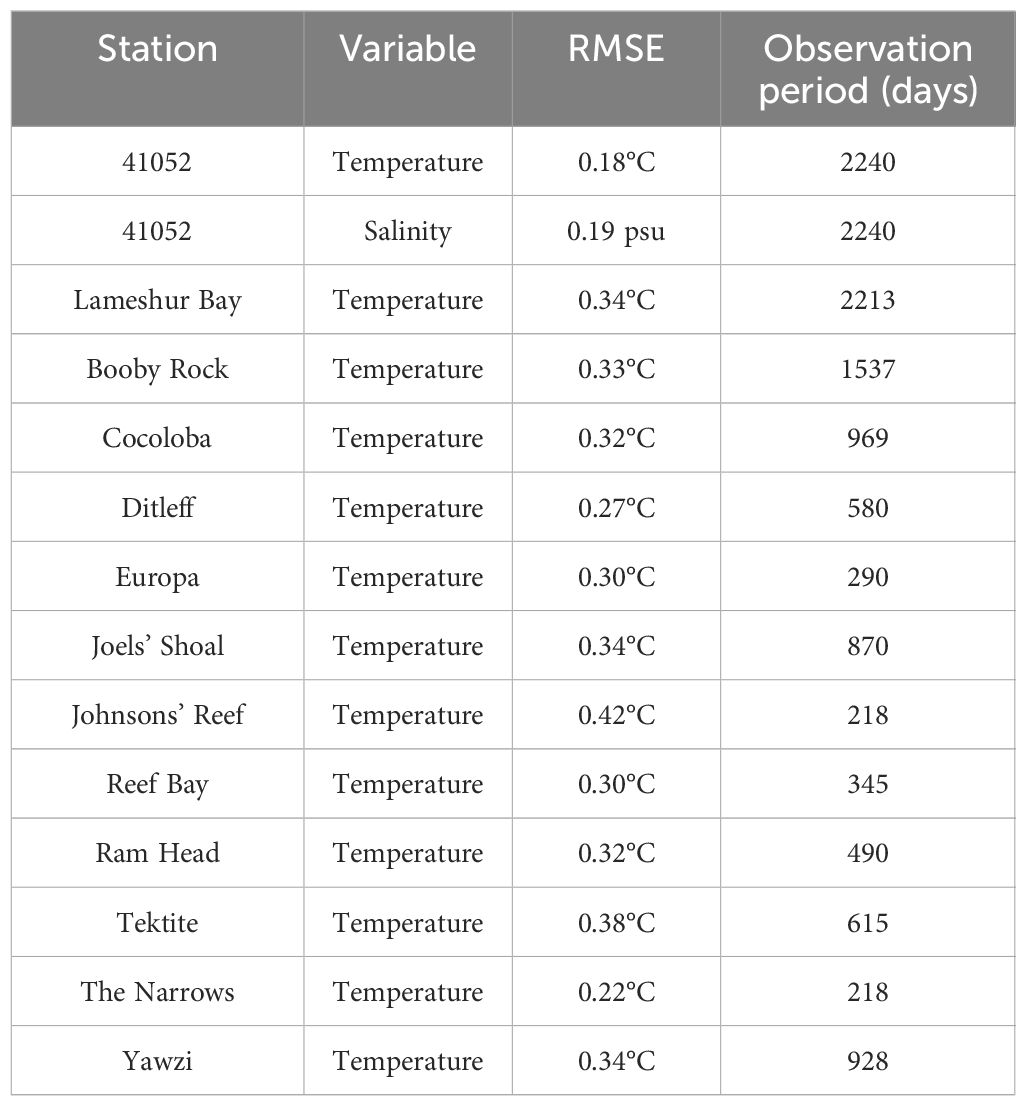
Table 1. Root-mean-square error (RMSE) of modeled temperature and salinity against observations at selected sites (locations marked on Figure 1).

To understand the influence of Amazon and Orinoco river plumes in the eastern Caribbean, daily sea surface salinity data from the NASA Soil Moisture Active Passive (SMAP) mission are used. These data have a spatial resolution of 0.25° but are noisy due to cloud cover. To obtain clear patterns of the river plumes, these data are averaged over the periods of Jun 15-Jul 15, 2021; Oct 15-Nov 15, 2021; Jul 15-Aug 15, 2022; and Oct 15-Nov 15, 2022.

3 Results

We quantify the spatial and temporal variability of flows, temperature, and salinity in the coastal region around St. John to characterize its physical environment, provide context for biological and biogeochemical studies, and informs ecosystem conservation efforts. All modeled hourly data presented here are instantaneous outputs at one-hour intervals.

3.1 Tides

The tides recorded at Lameshur Bay and The Narrows highlight both similarities and differences in tidal patterns on the south and north shores of St. John (Figures 2A, B). Pronounced spring-neap cycles are evident on both shores and remain synchronized. On the south shore (Figure 2A), diurnal oscillations dominate, with amplitudes reaching 0.2 m during spring tides and about 0.1 m during neap tides. A small semidiurnal component becomes noticeable only during neap tides. In contrast, the north shore (Figure 2B) exhibits a mixed semidiurnal pattern, with a spring tide amplitude of about 0.25 m.

Figure 2

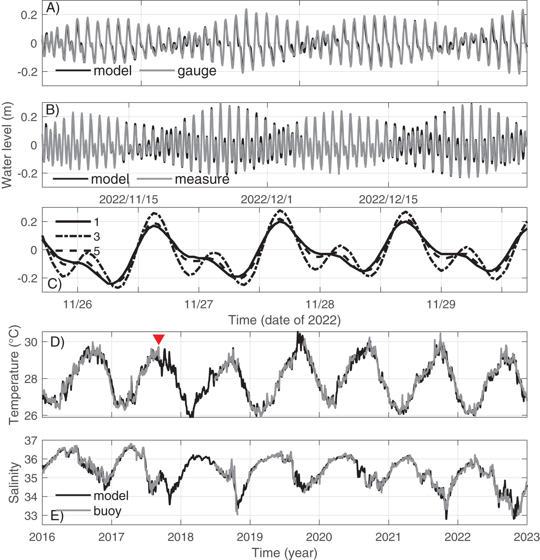
Figure 2. Time series of modeled and observed hourly water level at (A) the Lameshur Bay on the south shore and (B) the Narrows on the north shore from November 5 to December 31, 2022; (C) Time series of modeled hourly water level at different reef sites around St. John (see Figure 1C for locations) in Nov. 2022; Time series of modeled and measured daily mean (D) temperature and (E) salinity at NOAA Buoy 41052. The red triangle in (D) highlight the temperature drop induced by Hurricane Irma in September 2017.

The model captures tidal variations at both sites, including phase and amplitude differences (Figures 2A, B; 3A, B). The root‐mean‐square errors (RMSEs) of the modeled tidal elevation in the period of November 5, 2022, to January 7, 2023, are 0.024 m on the south shore and 0.025 m on the north shore (Figures 3A, B). At Lameshur Bay, the RMSEs of tidal elevation, subtidal water level, and total water level in the period of January 5, 2021, to December 31, 2022, are 0.02 m, 0.04 m and 0.05 m, respectively. Tidal comparison at Lameshur Bay is provided in Table 2.

Figure 3

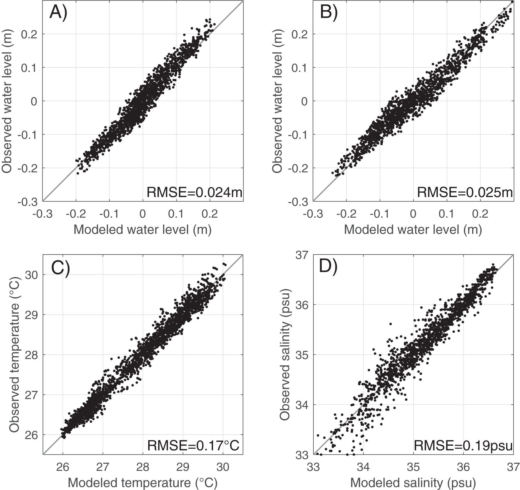
Figure 3. Scatter plots of observed vs. modeled water level at (A) Lameshur Bay on the south shore and (B) The Narrows on the north shore in the period of 2022-11–05 to 2023-01-07, and daily mean (C) near-surface temperature and (D) salinity at NOAA Buoy 41052 in 2016-2022.

Table 2

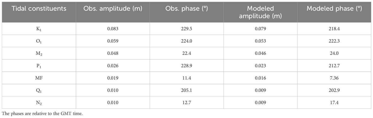
Table 2. Comparison of observed and modeled tidal constituents at Lameshur Bay in the period of May 01, 2021 to December 31, 2022.

The model shows that semidiurnal tides are more pronounced on the north shore, whereas diurnal tides dominate the south shore, including the southern end of the western channel (Figure 2C; sites marked in Figure 1C). Over a spring-neap cycle, the higher high water level on the north shore consistently exceeds the high water level on the south shore. The former may lead or lag behind the latter, but their time difference is always less than 1 hour (Figures 2A–C). Additionally, the lower low water on the north shore is consistently lower than that on the south.

Spatially, the M₂ tidal amplitude decreases from 0.14 m on the north shore to 0.04 m on the south shore, while the K₁ amplitude is relatively uniform around the island (Figure 4). The M₂ tides propagate northward through the channels on either side of St. John before converging on the north shore, and the north-to-south phase difference is about 15° (31 minutes). In contrast, the K₁ tides propagate southward, with a north-to-south phase difference of about 6° (24 minutes).

Figure 4

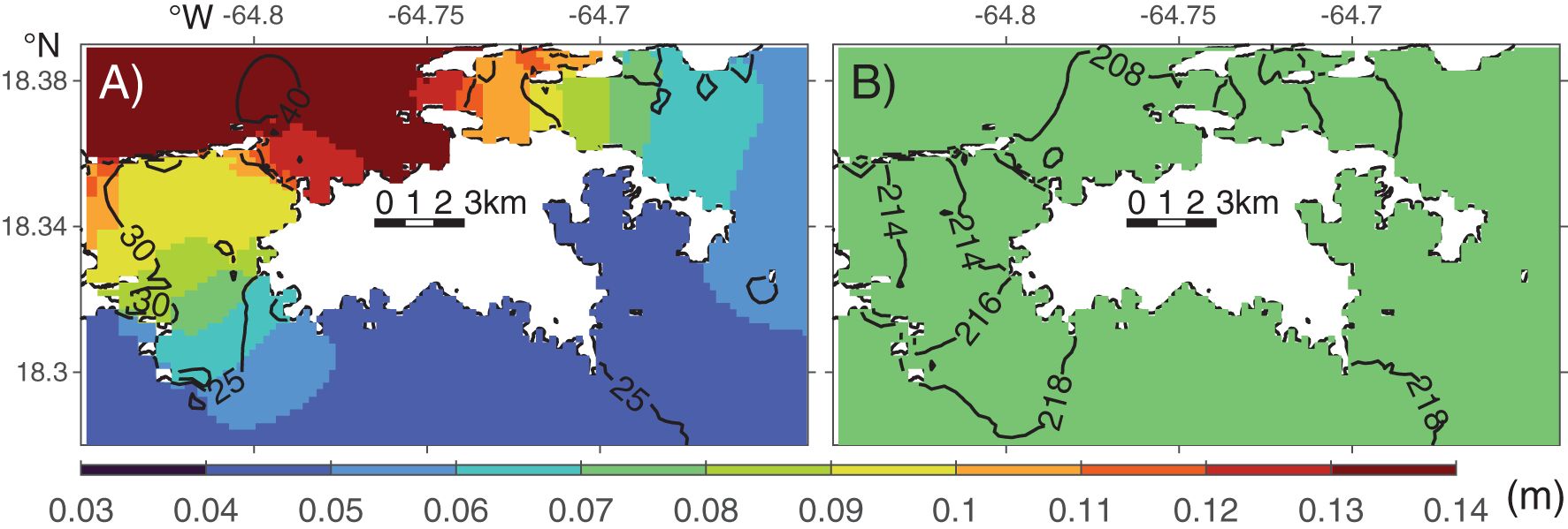
Figure 4. Modeled (A) M₂ and (B) K₁ tidal amplitude (color) and co-phase lines (black lines). The phase intervals are 5° and 2° in (A, B), respectively.

M₂ tidal currents in the western and northeastern channels are primarily along-channel, with maximum speeds of 0.90 m s^‐1 and 0.68 m s^‐1, respectively (Figure 5A). In contrast, K₁ tidal currents in the channels are much weaker, with a maximum surface speed of about 0.10 m s^-1 (not shown). Outside these channels, tidal currents on the southern open shelf and in coastal bays are 1‐2 orders of magnitude weaker. In particular, tidal currents in Coral Bay and Francis Bay remain weak despite tidal range there being comparable to the surrounding coast. Meanwhile, strong oscillatory tidal flows on the south shore interact with headlands, generating transient eddies, which are further examined in Section 3.4.

Figure 5

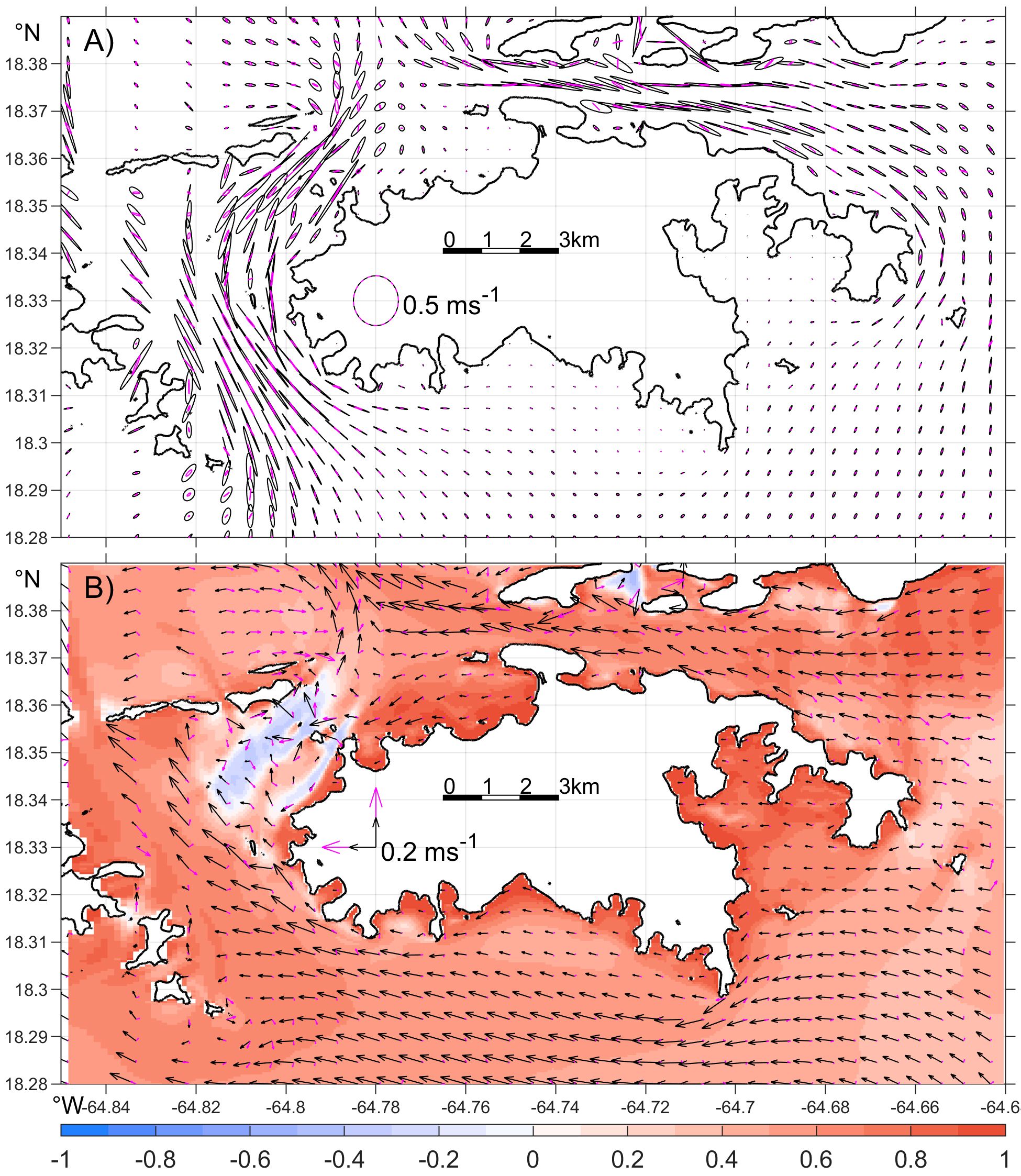
Figure 5. Modeled (A) surface (black) and bottom (magenta) M₂ tidal ellipses and (B) mean current in 2021-2022. The color in (B) represents the time-correlation between the daily mean zonal wind and the daily mean zonal surface velocity at each grid over the two-year period. Note that the scales of surface and bottom velocities are the same in (A) but different in (B).

3.2 Subtidal mean flows

Flows around St. John also vary over subtidal time scales. To establish a baseline pattern, we first examine modeled mean surface and bottom flows in 2021-2022 (Figure 5B). The mean surface flows around St. John are westward, consistent with the prevailing easterly wind (Figure 1B). On the southern shelf, surface mean flows range from 0.1 to 0.3 m s^‐1, stronger than the tidal flows. In the northeastern channel, the surface mean flows are westward at 0.1-0.2 m s^‐1, significantly weaker than the tidal currents. In contrast, the surface mean flows in the western channel are mostly northwestward, with a maximum speed of 0.3 m s^‐1, also weaker than local tidal flows.

Mean currents generally weaken with depth, with bottom flows across most areas are an order of magnitude weaker than surface currents. Within nearly all bays around St. John, mean currents are minimal, likely due to coastline sheltering and more effective bottom friction. The coastline impact is particularly pronounced immediately west of Ram Head (marked in Figure 1C), where the headland diverts the westward mean flow southwestward, leading to notably weak currents in the western adjacent waters (Figure 5B).

The model indicates that variations in surface subtidal mean flow around St. John are primarily wind-driven. To quantify this relationship, we compute the correlation coefficient between the daily mean zonal wind and the daily mean zonal surface flow at each grid point for 2021–2022 and obtain correlations exceeding 0.9 and R² values greater than 0.85 for most of the shallow near-shore regions (Figure 5B). The high correlation presumably reflects the impact of wind drag on the surface flow. That is, strong easterly winds tend to drive strong westward surface flows. On the south shelf and in the northern channel, the correlations reduce to 0.50-0.75, and the corresponding R² values are 0.15-0.50. These reduced correlations suggest that other factors, such as flow interactions with topography, exert stronger influence on the surface currents there than the near-shore regions.

Different from most of the coastal region, the northern part of the western channel shows a negative correlation of about –0.3 with R² values of 0.05-0.1. That is, strong easterly winds correspond weakly to strong eastward flows there. Consistent with the tidal asymmetry on the north and south shores, sea level in the northern part of the channel has a mean southward drop, and mean flows there are southwestward with peak flows concentrated in the gaps between small islands, such as Henly and Rata Cays (Figure 6C). To understand the mechanism behind the negative correlation, we examine details of the flow pattern there and find that wind fluctuations modify local flows by altering sea level tilt there. For illustration, we examine the difference in water levels at Point P1 inside and P2 north of the channel (Figure 6C) over March 26 - April 4, 2022. During the period, winds are persistently westward but weaker in the first than the last 4 days (Figure 6A). In the first 4 days, both the subtidal water levels drop from P2 to P1 and the subtidal mean southwestward flow strengthen (Figures 6B, D). In contrast, in the last 4 days with strong westward winds, the southward water level drop diminishes, and the southwest flow weakens (Figure 6E). Closer examination of the model field indicates that the wind impact on sea level spans over the larger coastal region and is consistent with coastal upwelling and downwelling associated with wind-driven Ekman transport. Essentially, strong easterly wind strengthens coastal upwelling and raises sea level on the south shore, and it also strengthens coastal downwelling and suppresses sea level on the north shore. The sea level variations propagate into the western channel and reduce the southward mean sea level drop there. The opposite effect occurs when the easterly wind weakens. These together give the negative correlation between the zonal wind and the local mean flow.

Figure 6

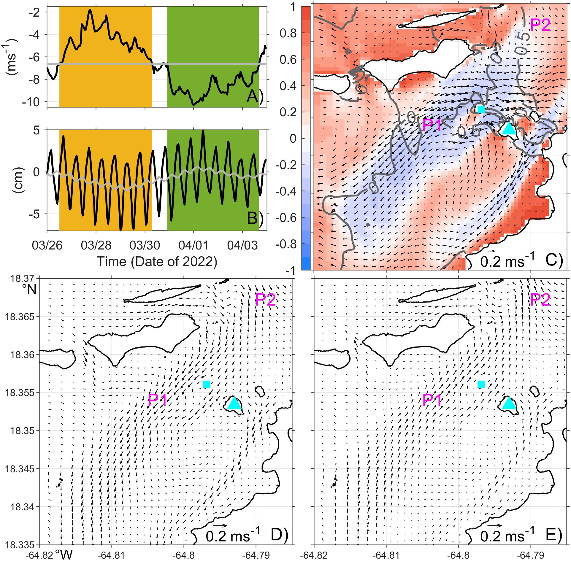
Figure 6. Time series of (A) hourly (black) and long-term mean (gray) zonal wind speed, and (B) hourly (black) and daily mean (gray) water level difference between Points P1 and P2 (P1-P2) from March 26 to April 4, 2022. Periods of weak and strong easterly winds are highlighted by orange and green shading, respectively. (C) Plane view of surface mean velocity (arrows) and water level (gray contours, with 0.5 cm interval) over March 26 to April 4, 2022, overlaid with the 2-year time-correlation between zonal wind and surface velocity (color). Plane view of surface velocity anomaly relative to the time mean velocity during weak (D) and strong (E) easterly wind periods. Locations of P1 and P2 are marked in (C–E). The cyan triangle and square mark Henly Cay and Rata Cay, respectively. Note that the vector scale in (C) differs from (D, E).

3.3 Temperature and salinity distribution

Daily mean near-surface temperature and salinity from the NOAA buoy 41052, south of St. John, exhibit pronounced seasonal and interannual variations (Figures 2D, E). The temperature variation is dominated by the seasonal signal with summer-to-winter temperature difference of 3-4°C. The salinity variations are more irregular with strong fluctuations and secondary maxima and minima in most of the years. The model successfully captures these seasonal and interannual patterns observed at the buoy, with RMSEs of 0.17 °C for temperature and 0.19 psu for salinity (Figures 3C, D). RMSEs of the modeled bottom temperature on the south shore (Figure 1C, colored symbols) compared to scattered in situ observations in 2016–2022 range from 0.22 to 0.42 °C (Table 1).

We now focus on the spatial and temporal variability of modeled temperature and salinity around St. John. Monthly mean surface temperature and salinity in March and September 2021 (Figures 7, 8) are used to illustrate spatial variability at seasonal extremes, which are largely consistent across the model years.

Figure 7

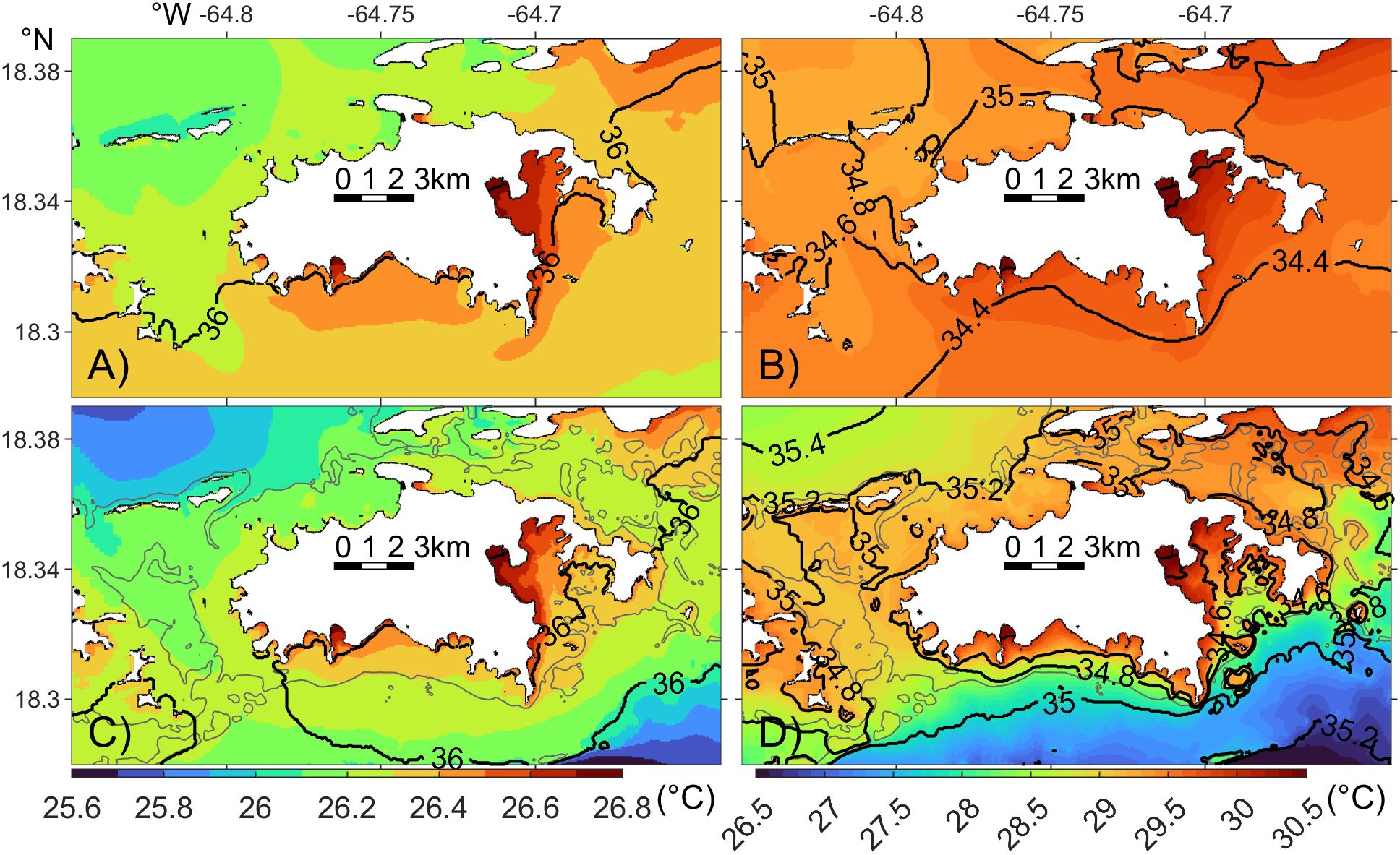
Figure 7. Monthly mean surface (A, B) and bottom (C, D) temperature (color) and salinity (black contour, 0.2 psu interval) in March (A, C) and September (B, D) 2021. Note that the color axes change between months, but the interval of the color contours is fixed at 0.1°C. The gray lines in bottom panel denote the 25 m isobath contour.

Figure 8

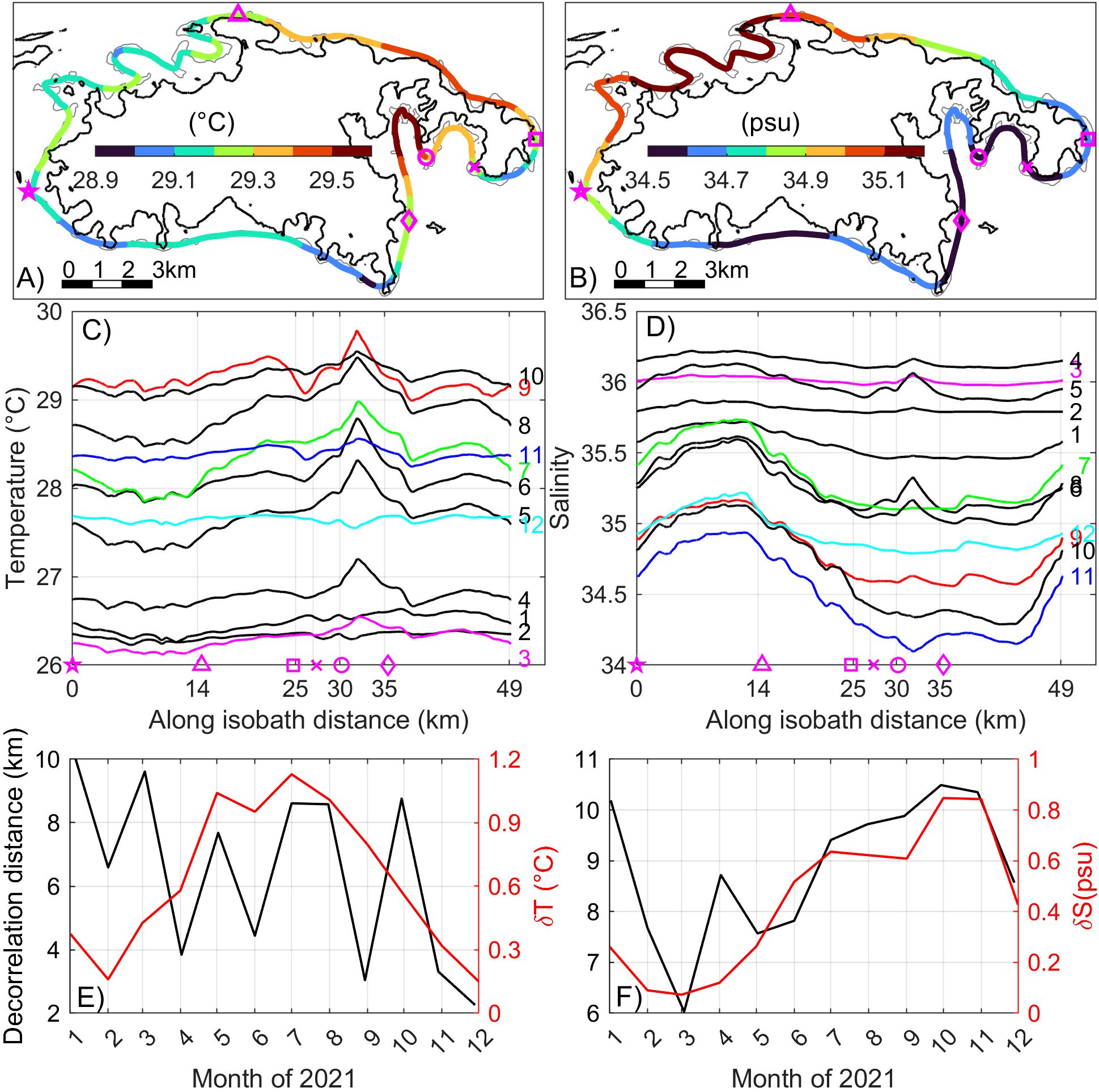
Figure 8. Plan view of monthly mean bottom (A) temperature and (B) salinity along the smoothed 16-m isobath contour in September 2021; Monthly mean along 16-m isobath bottom (C) temperature and (D) salinity in 2021; Time series of monthly (E) temperature and (F) salinity decorrelation distance (black) and the corresponding along-isobath variation range (red) in 2021. The magenta symbols in (A, B) correspond to the sites highlighted in (C, D); In (C, D), colored numbers to the right denote months.

3.3.1 General variability in space

In March 2021, surface temperature around St. John show minimal variation, ranging from 26.1°C to 26.8°C (Figure 7A). Temperature increases from the north shore toward the south, with the coldest waters along the northwest coast and the warmest in Coral Bay, southeast of the island. Some of the cooler water is advected from the northwest coast into the western channel by tidal flows. Meanwhile, bottom temperature inshore of the 25 m isobath closely match the surface temperature (Figure 7C), indicating minimal stratification in the shallow coastal regions. Beyond the 25 m isobath, bottom temperatures gradually decline relative to the surface, indicating thermal stratification in the deeper shelf regions.

Surface salinity around St. John remains relatively uniform in March, ranging from 35.9 psu on the southern shelf to 36.1 psu along the north shore and 36.2 psu in Coral and Fish Bays (Figure 7A). Salinity along the St. John coastline varies by only 0.3 psu. The slightly higher salinity on the north shore compared to the south is consistent with the salinity contrast between the Sargasso Sea to the north and the Caribbean Sea to the south (Chollett et al., 2012). The highest salinity is observed in Coral Harbor, located at the northern end of Coral Bay (Figure 1C), where salinity is 0.2 psu higher than the nearby shelf salinity. This increase corresponds to an 8.5% higher evaporation rate in the model. Bottom salinity around the island closely resembles the surface values (Figure 7C).

The spatial pattern of surface temperature in September closely resembles that of March (Figure 7B). However, September temperatures, ranging from 29.3°C to 30.5°C, are higher and exhibit greater spatial variability than those in March. Bottom temperatures also closely match surface temperatures inshore of the 25 m isobath (Figure 7D). Beyond that, bottom temperatures gradually decrease relative to the surface temperatures, with the difference increases farther offshore, particularly on the southern shelf. At 5 km to the south of the island, bottom temperatures are ~2°C lower than surface temperatures.

Surface salinity in September ranges from 34.3 and 35.1 psu, generally lower than in March, but with a larger spatial variation of 0.8 psu (Figure 7B). Salinity in September also decreases southward, consistent with the large-scale salinity changes. The highest salinity is observed in Francis Bay, north of the island, where modeled evaporation rate is high. On the south shore, salinity in Coral Harbor and Fish Bay remains the highest, reaching 34.8 psu, about 0.5 psu higher than the surrounding shelf waters. Correspondingly, modeled evaporation rates are 39% and 32% higher than those on the south shelf. The lower salinity along the south shore is attributed to the intrusion of fresher Amazon and Orinoco River plumes from the south through the model open boundary conditions extracted from HYCOM (Section 3.3.4). Bottom salinity around the island in September differs noticeably from surface salinity, except in near-shore regions (Figure 7D). The difference increases toward offshore. Along the 25 m isobath, bottom salinity is 0.4-0.6 psu higher than at the surface. This difference primarily reflects the influence of the river plumes, which will be examined in Section 3.3.4.

3.3.2 Alongshore variability

To quantify the reef-scale variability and provide quantitative information on the variation length scale for conservation efforts, we examine the alongshore distribution of bottom temperature and salinity in 2021. The 16-m isobath contour around St. John is selected here as it traverses much of the regions with relatively high benthic coral coverage (10%-50%) (Zitello et al., 2009). Both the original 16-m isobath and the bottom temperature along the original 16-m isobath are spatially smoothed with a running average window of 2 km (Figure 1C, red dashed line) to reduce the large-amplitude zigzag pattern of the isobath contour and also to obtain a continuous space series for subsequent spatial decorrelation calculation.

We first use September 2021 as an example to illustrate the alongshore variability and then analyze statistics of the variability in the other months. The alongshore distribution of bottom temperature in September (Figure 8A) exhibits a pattern opposite to that of surface temperature: bottom temperatures are generally warmer on the north shore than on the south. This is driven by the relaxation of easterly winds in September 2021, which facilitated the onshore intrusion of cooler shelf water along the south shore (Section 3.3.4). Around the entire island, Coral Bay has the highest bottom temperature, while the water immediately west of Ram Head has the lowest (Figure 8A). These localized bottom temperature extrema occur within the bays over length scales of 1~3 km, whereas bottom temperature variations along open shoreline occur over a length scale of ~5 km.

Statistical analysis of the annual variation in the monthly mean alongshore bottom temperature (Figure 8C) indicates that from January to March, the maximum alongshore temperature difference is relatively small, around 0.4°C (Figure 8E, red line). During this period, the decorrelation length scale—defined as distance over which spatial autocorrelation of the alongshore temperature decreases to e^-1—ranges 7–10 km (Figure 8E, black line). Notably, these decorrelation length scales remain largely unchanged when using daily mean temperature instead of monthly mean.

In contrast, from May to September, the northeast coast and Coral Bay experience more pronounced warming compared to the rest of the coastline. During this period, the maximum alongshore temperature difference increases by 0.5~0.9°C, while the alongshore decorrelation length scale decreases to 3~8 km. This indicates that hydrographic variability at the bottom is higher in summer than in winter.

The alongshore variation in bottom salinity in September (Figure 8B) closely follows the pattern observed in surface salinity (Figure 7B), with the highest salinity along the northwest coast and the lowest along the south and southeast coasts. On the seasonal timescales, the alongshore difference in bottom salinity ranges from 0.1 to 0.4 psu between December and May, increasing to 0.5-0.8 psu from June to November (Figures 8D, F). The decorrelation length scale for bottom salinity remains relatively stable at 8–10 km throughout most of the year, except in March when it decreases to 6 km (Figure 8F), though with a smaller overall variation. Unlike bottom temperature, alongshore bottom salinity shows no significant bay-scale variability. This is consistent with the absence of local river input, as the seasonal freshening along the south shore primarily results from large-scale intrusions of remote river plumes from offshore (section 3.3.4).

3.3.3 Cross-shore variability

The monthly mean temperature and salinity in March and September are analyzed along five cross-shore transects located to the west, northwest, north, south, and southeast of the island (marked in Figure 1C) to illustrate the general cross-shore variation of hydrographic conditions. Note that the spatial variation patterns of monthly mean temperature and salinity are similar to those of daily mean.

In March, temperature and salinity distributions along most transects exhibit minimal cross-shelf and vertical variability (Figures 9A, C, E, G, I). The lack of vertical variation aligns with the previously noted similarity between surface and bottom temperatures in nearshore regions (Section 3.1). It indicates that the coastal water is generally well-mixed during this period. The only exception is along the southeast transect across Coral Bay (Figure 9I), where temperature and salinity are slightly higher in the shallower bay end, primarily driven by solar radiation and evaporation (Section 3.3.1). Temperature and salinity variations along the sloping bottom on the transects to the west, northwest, north and south of the island are negligible. Even along the 3-km southeast transect, the maximum along-bottom temperature and salinity change are only 0.5°C and <0.1psu, respectively.

Figure 9

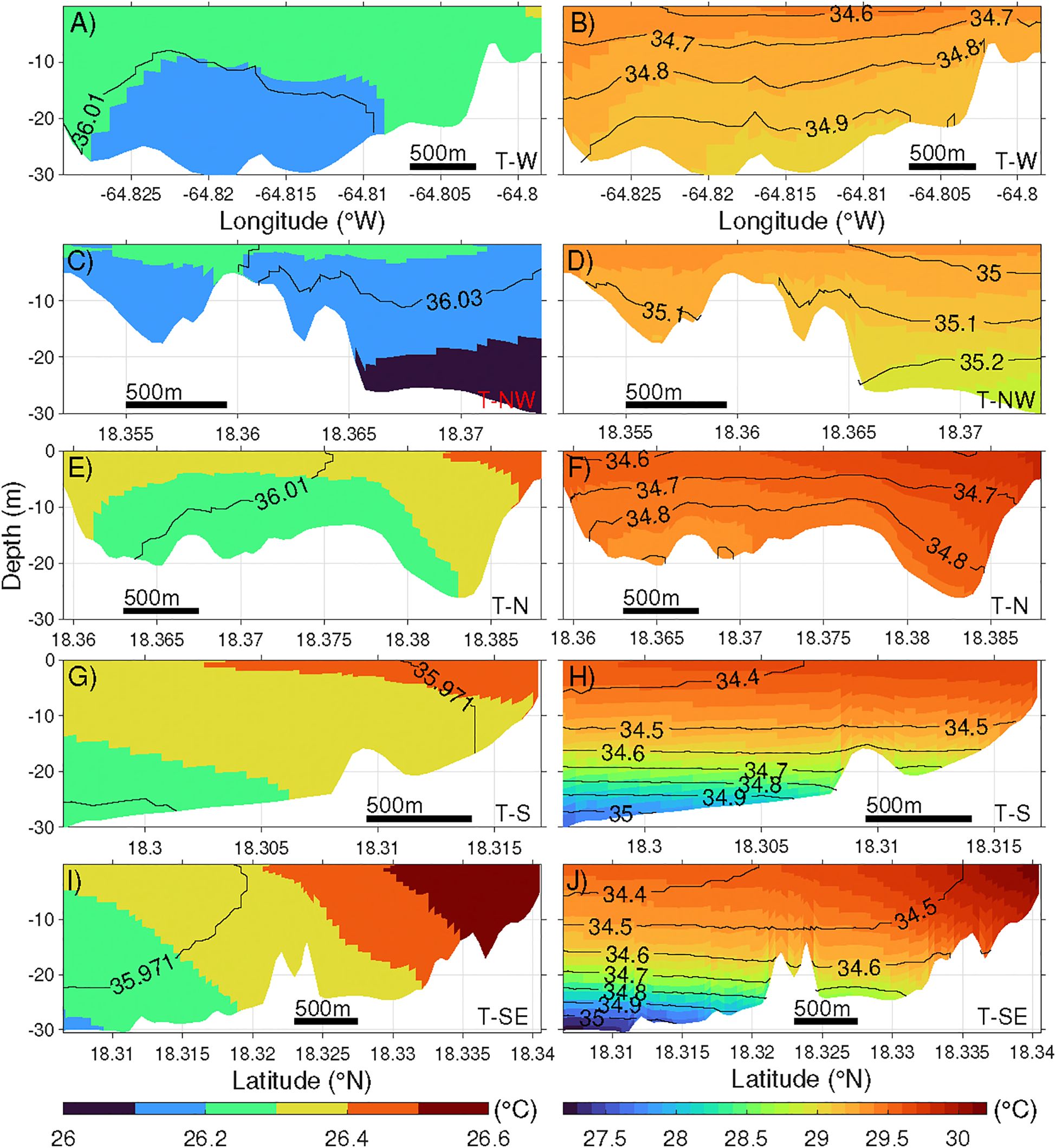
Figure 9. Cross-shelf sections of monthly mean temperature (color) and salinity (black contour, 0.1 psu interval) in March (A, C, E, G, I) and September (B, D, F, H, J) 2021. Note that the color axes change between months, but the interval of the color contours is fixed at 0.1°C. Location of the sections are marked as orange lines in Figure 1C. The thick black bar represents a length of 500 m.

In September, temperature and salinity on all transects show pronounced vertical changes, and the cross-shelf changes are relatively small (Figures 9B, D, F, H, J). On the south and southeast transects, temperature decreases by 2-2.5°C and salinity increases by 0.4-0.6 psu in 30 m depth range, both greater than the changes on other transects.

3.3.4 Temporal variability

At all five representative sites along the 16-m isobath (Figure 1C), modeled bottom temperature exhibits a clear seasonal cycle, reaching its annual maximum in late September to early October and minimum in February to March (Figure 10A). This pattern aligns with the surface temperature variations observed at the offshore buoy (Figure 2D).

Figure 10

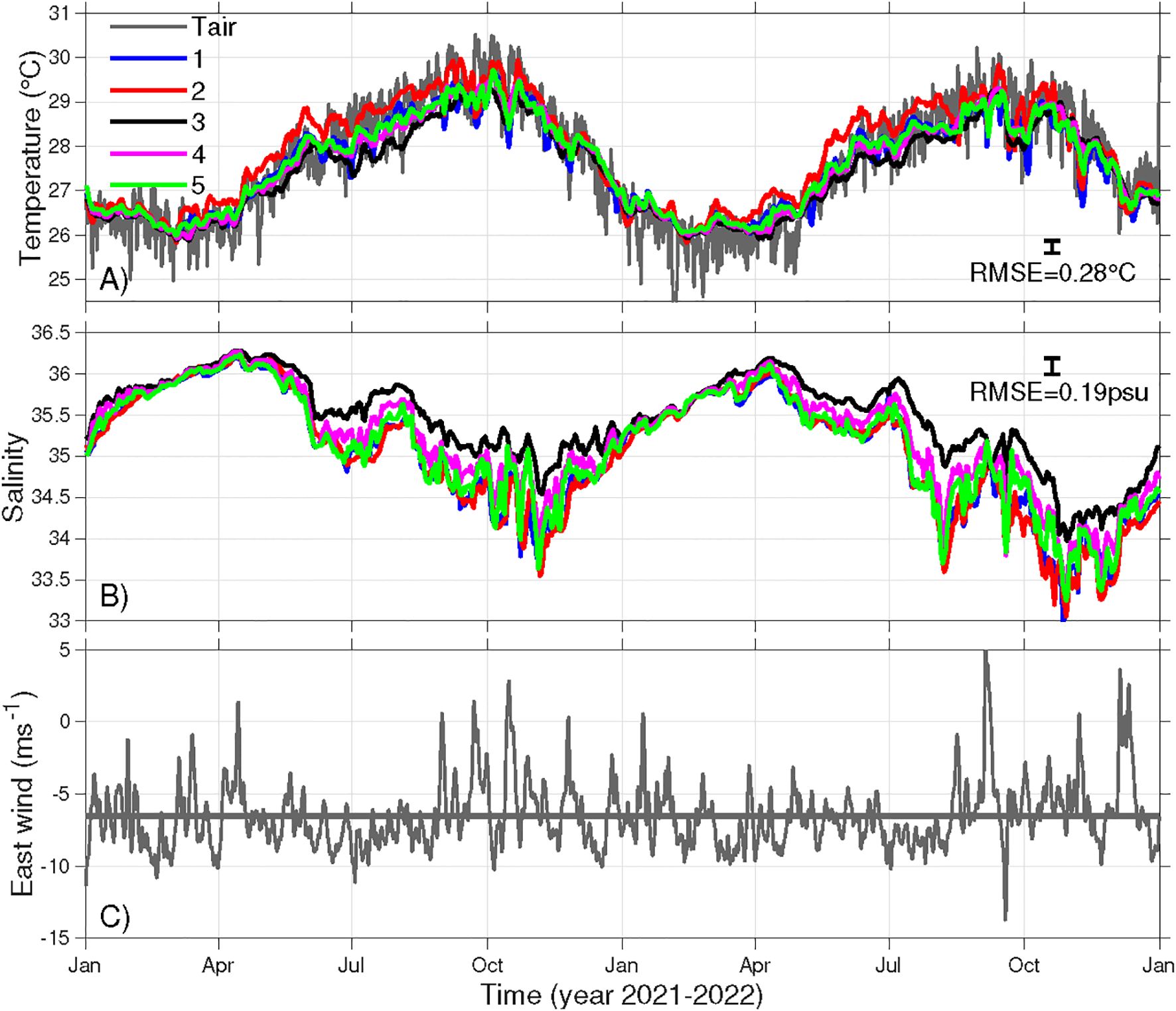
Figure 10. Time series of observed daily mean surface air temperature and modeled ocean bottom (A) temperature and (B) salinity at Sites 1-5 (marked in Figure 1C), and (C) observed daily mean zonal winds. Thick gray line in (C) is the 2-year mean zonal winds from NOAA Buoy 41052. The vertical bars in (A, B) show the maximum RMSE of modeled bottom temperature and that of near-surface salinity, 0.28 °C and 0.19 psu, respectively, for reference.

During the warming season (April-September), bottom temperatures show some spatial differences, with Site 2 (in Coral Bay) warming the earliest and maintaining temperatures ~0.5°C higher than the other sites. In contrast, during the cooling season (October-February), temperatures decrease consistently across all sites. Additionally, the bottom temperature shows fluctuation in timescales of 2–5 days, presumably reflecting the influence of weather events (Figure 10C).

Notably, during the warmest period (August to early November), Sites 1, 2, and 5 (all on the south shore) experience episodic temperature drops of 0.5-1.5°C. These events coincide with episodically relaxed easterly winds. A 20-day sensitivity simulation with the relaxed easterly winds replaced with a long-term mean easterly wind of 6.5 ms^-1 shows much less temperature fluctuations. This confirms that the fluctuations at least partially result from episodic relaxation of easterly winds, which weakens the onshore Ekman transport of warm offshore surface waters on the south shelf and allows cooler subsurface shelf waters to intrude along the bottom toward the south shore.

At all five sites, bottom salinity follows a clear and synchronized seasonal cycle, peaking in mid-April and reaching its annual minimum in November (Figure 10B). From November to April, salinity increases in a mostly monotonic manner with minimal fluctuations. However, the seasonal freshening after April occurs in two distinct stages, ultimately leading to the lowest in late October. The first stage of freshening occurs before July, followed by a brief period of rising salinities at all sites. The second stage, from August to November, is marked by large-amplitude oscillations, particularly at Sites 1, 2, 4 and 5 on the south shore. In contrast, Site 3, on the north shore, experiences a much smoother freshening trend. As a result, the maximum salinity difference between Site 3 and the other sites exceeds 1 psu at times.

Analysis of satellite-measured sea surface salinity suggests that the temporal variation of salinity along the St. John coast is strongly influenced by the Orinoco and Amazon river plumes. Sea surface salinity imagery confirms that, after passing through the Lesser Antilles from the east, the Amazon River plume reached St. John in July 2021 and 2022 (Figures 11A, C). Similarly, the Orinoco River plume traversed the Caribbean Sea and arrived the southern shelf of St. John in October of both years (Figures 11B, D). These staggered arrivals correspond to the two distinct stages of freshening observed in the shelf waters south of St. John (Figure 10B). Our analysis further suggests that interannual variability in seasonal freshening is linked to differences in dispersal patterns of the Amazon and Orinoco plumes. For example, the Orinoco River plume was fresher in 2022 than 2021 (Figure 11), consistent with lower salinity minima at all selected coastal sites in 2022 compared to 2021 (Figure 10B).

Figure 11

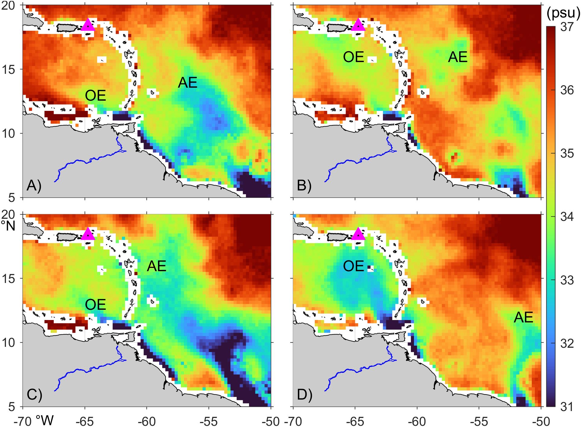
Figure 11. Temporarily averaged surface salinity from SMAP. The corresponding average periods are (A) Jun 15-Jul 15, 2021, (B) Oct 15-Nov 15, 2021, (C) Jul 15-Aug 15, 2022, and (D) Oct 15-Nov 15, 2022. Gray color marks the land. Blue lines mark the Orinoco River. Magenta triangle marks St. John. OE and AE denote the Orinoco and Amazon River plume extensions, respectively.

3.4 Headland eddies

A particular type of hydrodynamic variability in the St. John coastal region is transient eddies generated by oscillatory tidal flows interacting with headlands. These eddies can affect the dispersal of coral and fish larvae. The St. John model shows headland eddies at Ram Head (Figure 12) and Ditleff Point (not shown). Here, we use Ram Head headland eddies to demonstrate the associated hydrodynamic variability. When the westward tidal current reaches Ram Head (Figure 1C), it is deflected southwestward and generates an anticyclonic (clockwise) eddy with negative relative vorticity on the downstream (west) side of the headland (Figure 12A). This eddy then moves downstream with the current, expanding in diameter from approximately 500 m to 1 km, and gradually disappearing in a few hours. A cyclonic (counterclockwise) eddy with positive relative vorticity is formed on the east side of Ram Head during an opposite phase of the tide (Figure 12B).

Figure 12

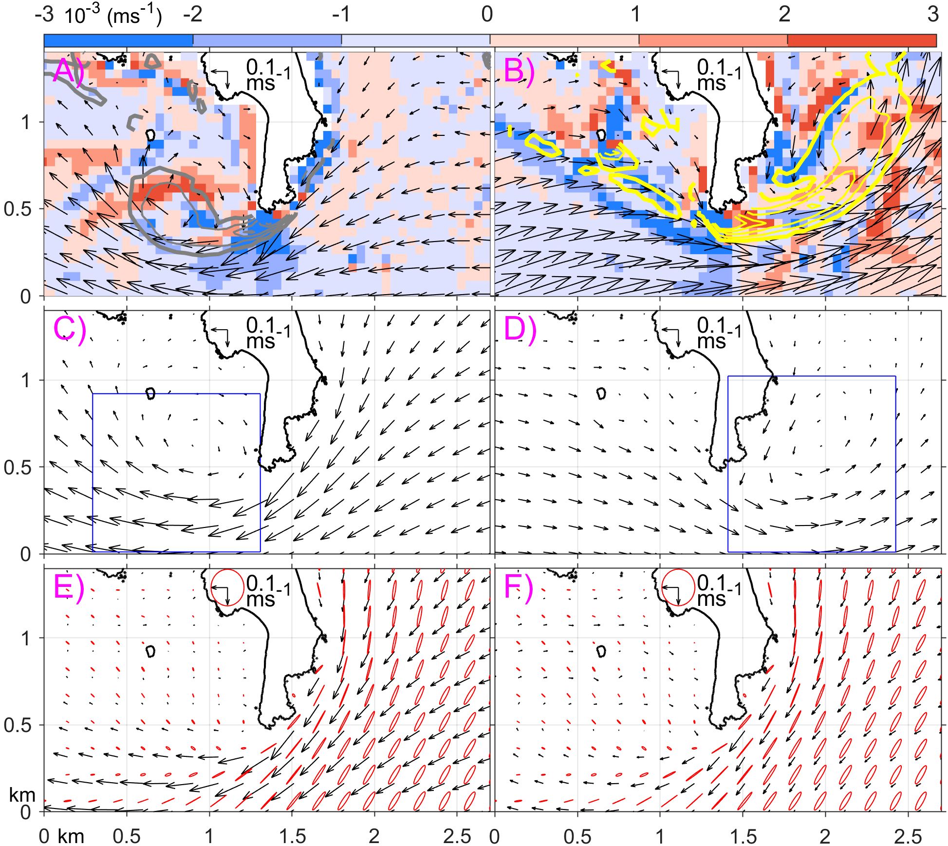
Figure 12. Snapshot of headland eddies around Ram Head at (A) 2022/11/08 9:00 GMT and (B) 2022/11/06 7:00 GMT. Composite average of the horizontal velocity (arrows) at times with an eddy presented to the (C) west and (D) east of Ram Head. Averaged horizontal velocity (arrow) during (E) December-August, and (F) September-November. All horizontal velocities are at 5 m depth. In (A, B), color denotes vertical velocity; thick grey and yellow contours denote relative vorticity of 0.5×10³ and -0.5×10³ s^-1, respectively, and the corresponding thin contours represent relative vorticity with the interval of 1×10³ s^-1. The blue rectangles in (C, D) mark the regions for eddy detection. Red ellipses in (E, F) denote M₂ tidal ellipses during 2021-2022.

Signell and Geyer (1991) explained the formation mechanism of the tidally driven headland eddies. Using the westward tidal flow as an example, as the upstream (east) side of the headland coast directs the incoming tidal flow southward toward offshore, the coastal boundary layer flow accelerates due to volume conservation. The boundary flow reaches its maximum speed at the tip of the headland, where the cross-shore displacement of the flow is the greatest. Due to the Bernoulli effect, pressure at the headland tip decreases lower than the pressure along the western coast of the headland. This creates a southeastward pressure gradient along the downstream (west) coast of the headland. As a result, the incoming boundary flow from east separates from the coast at the headland tip. This separated flow transports relative vorticity from the boundary layer into the lee (west) side of the headland, forming a transient eddy. The same mechanism occurs during the opposite phase of the tide and generate an eddy to the east of the headland. The modeled currents also shows strong convergence or divergence and localized strong vertical velocity on the order of 10 m hr^-1 in the eddies (Figures 12A, B).

To quantify this temporal variability of the headland eddy, we apply an eddy autodetection algorithm (Isern-Fontanet et al., 2006) and calculate the stream function and Okubo-Weiss parameter, $W={(\partial u/\partial x+\partial v/\partial y)}^2+4[(\partial u/\partial y)(\partial v/\partial x)-(\partial u/\partial x)(\partial v/\partial y)]$ using modeled hourly horizontal velocity at a depth of 5 m (e.g., Figures 13A, B). Here, u and v represent the zonal and meridional velocity components, respectively. Unlike its applications in mesoscale eddy studies (e.g., Chelton et al., 2007; Du et al., 2022), here horizontal divergence is included in the small-scale headland eddies. Tests indicate that this divergence does not significantly impact the W value. An eddy is identified as closed stream function contours within the ~1 km² rectangle regions to the immediate west and east to the headland (Figures 12C, D, blue rectangles) with $W<-3\times {10}^{-7}$s^-2. Eddies occurring over consecutive time records are considered single eddies, while those with time gaps are considered separate.

Figure 13

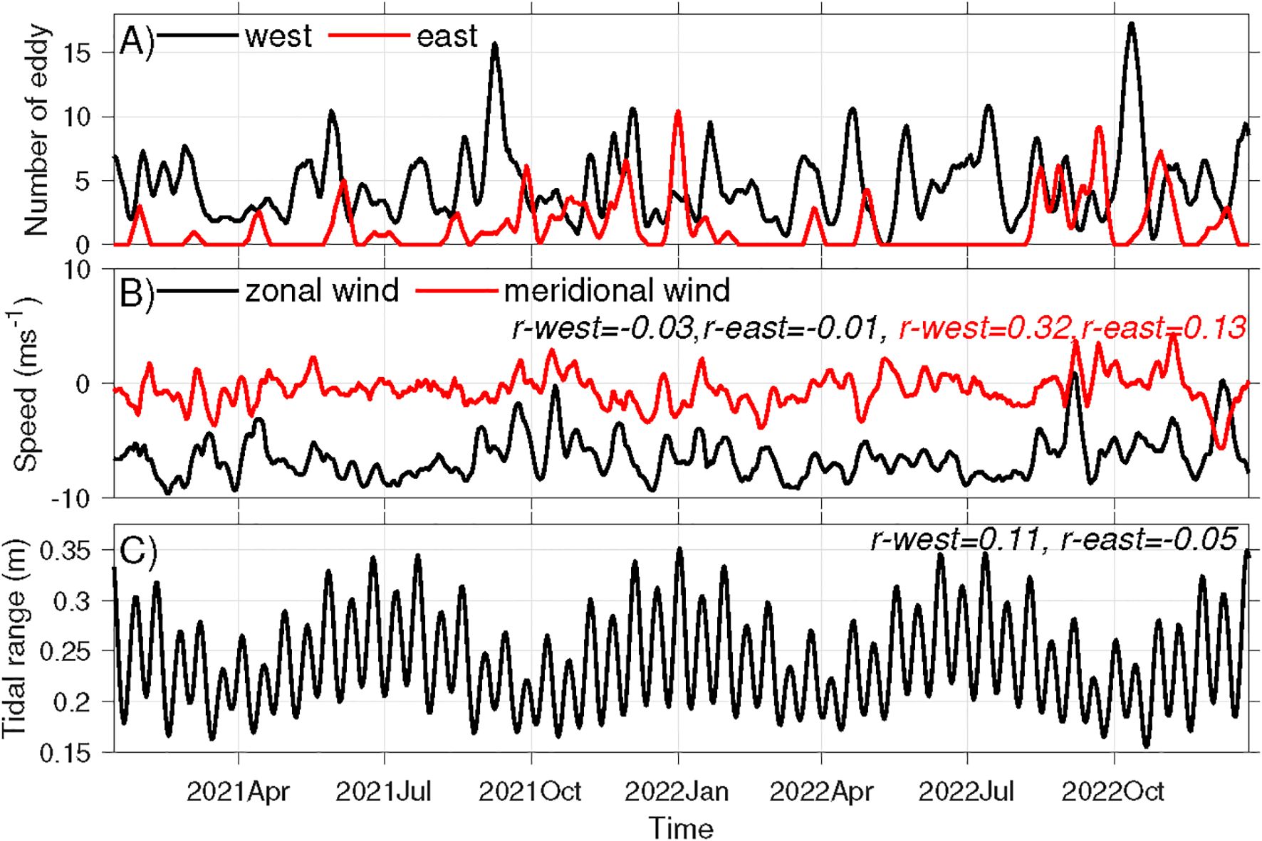
Figure 13. Time series of weekly (A) numbers of headland eddies formed to the west and east of Ram Head, (B) mean zonal and meridional wind, and (C) mean tidal range at Site 1 in 2021-2022. Numbers at the upper right corners of (B, C) denote correlations of the corresponding variables in the panels with the weekly eddy number to the west and east of Ram Head in (A). Note that all correlations reported here are insignificant with p-values greater than 0.05.

Even though the tidal flows are oscillatory, eddies generated on the opposite sides of the headland exhibit spatial asymmetry. Over the 727 model days in 2021–2022, 496 eddies were identified to the west of Ram Head, while only 132 were identified to the east. Meanwhile, 68% and 18% of the days have eddies present to the west and east of the headland, respectively, suggesting that the west side is more favorable for eddy formation. On average, eddies remained within the detection region for 1.6 hours on the west side and 2.3 hours on the east side. Composite average of the flow fields at time of the eddies reveal that the deflecting flow at the headland tip is stronger for western eddies than for eastern ones (Figures 12C, D). The weekly total eddy count indicates that most east-side eddies form in fall (September-November), with very few occurring in spring and summer (Figure 13A). In contrast, eddies on the west side form throughout the year.

To determine the mechanisms driving these spatial and temporal variations, we examine tidal currents and subtidal mean currents around the headland. Note that the M₂ tidal currents dominate the region, while the K₁ and O₁ tidal currents are an order of magnitude weaker. From December to August, when the winds are persistently westward (Figure 10C), mean currents to the east of the headland are westward with speeds exceeding M₂ tidal currents (Figure 12E). That is, the tidal currents cannot reverse the flow direction. Therefore, no eddy forms to the east of the headland. From September to November, with frequent relaxations of the easterly winds (Figure 10C), the westward mean currents east of the headland become weaker than tidal currents (Figure 12F). This allows tidal currents to overcome the mean flow and form eddies on the east side. Therefore, the seasonal variation of the wind appears to have a strong impact on the headland eddy formation.

The number of eddies on both sides of Ram Head are positively correlated with the weekly-mean meridional wind (Figure 13B). But the correlations are insignificant. This indicates that northward winds may enhance the formation of the eddies on both sides. The number of eddies on both sides shows negligible correlation with the weekly mean zonal winds (Figure 13B) and the weekly mean tidal range (Figure 13C). These suggest that zonal winds and tides have a minimal impact on eddy formation on the weekly time scale. The detailed dynamics of winds and tides impacting headland eddy formation is left for future studies.

4 Discussion

Variabilities in the physical environment of tropical marine ecosystems plays a critical role in the development, growth and resilience of the communities they support. A fine-scale understanding of water temperatures, salinities, and local flow features are vital to coastal resource management, such as coral reef restoration. However, such high-resolution information is often inaccessible, and policy makers and practitioners have to rely on lower resolution and offshore data that do not capture the fine-scale heterogeneity created by the interaction of coastal flows with complex reef topography and coastlines (Saint-Amand et al., 2023). There is thus a strong need for high-resolution hydrodynamic modeling of reef systems to resolve small-scale physical processes and integrate other fine scale interdisciplinary datasets to improve our understanding of how physical drivers influence biota in situ (Mooney et al., 2020; Apprill et al., 2023).

St. John, US-VI provides an ideal setting for such an endeavor. The long-term and ongoing ecological projects in the area (Friedlander and Beets, 2008; Miller et al., 2009; Tsounis and Edmunds, 2017; Edmunds, 2021) and the protected status of the island makes it an intriguing area to test the physical and biological integrated approach to understand and predict changes in biological processes, e.g., larval dispersal and pollution levels. The high computational demand of the high-resolution models underscores that this area in the short term can be used as a test site for in-depth understanding of the biophysical processes. For this purpose, we develop a high-resolution numerical model to simulate the coastal hydrodynamic environment around St. John. The model captures the majority of the observed variabilities of tides, temperature, salinity, and currents across multiple timescales, even though some residual errors remain. The model reveals significant heterogeneity in local oceanographic conditions, primarily driven by three main factors: winds, tides, and river plumes.

Winds exert a strong influence on the flows in the coastal region. For instance, the easterly winds tend to trap water in Coral Bay and Fish Bay, resulting in relatively high temperature and salinity there (Figures 7, 8). Weather-scale fluctuation of the winds also drives strong temporal variation of temperature, salinity and flows in the coastal region (Figure 10). Winds are also a major driver of the water exchange between the bays and open coast, which will be examined in Part II (Jia et al., 2025). Notably, several hurricanes passed through the model domain during the simulation period, and the model captured disturbances induced by the hurricanes, including a 1.5°C drop in surface water temperature on the south shelf following the passage of Hurricane Irma in September 2017 (red arrow in Figure 2D). Detailed impacts of hurricanes are left for future studies.

Unlike wind-driven influences, the effects of river plumes and tides are not as ubiquitous. The Amazon and Orinoco River plumes intrude into the region during summer and fall, modifying hydrodynamic conditions along the south shore. For instance, the arrival of plume waters reduces salinity on the south shore by about 1 psu (Figure 11B), similar to the finding of Johns et al. (2014) in 2009 and 2010. Meanwhile, Johns et al. (2014) also found that waters on the south shore during that time contained anomalously high concentrations of mesopelagic fish larvae but low concentrations of larvae from inshore and reef source regions. This aligns with finding of López et al. (2013), who reported that river plumes delivering nutrients and fish larval to the coastal region south of St. John.

Meanwhile, the model shows no clear plume influence on the north shore. Therefore, the river plumes may create distinct hydrodynamic and biogeochemical differences between St. John north and south shores. Furthermore, the intermittent arrivals of the plumes can alter the exchange flows between bays on the south shore and the open shelf, generating spatial and temporal heterogeneity in the coastal environment at even smaller scales (see Part II).

Tides affects flows in the St. John coastal region across multiple scales. The tidal asymmetry between the north and south shores—where semidiurnal tides dominate in the north and diurnal tides prevail in the south—drives strong tidal flows through the channels. Tidal flows can also interact with headlands, such as Ram Head and Ditleff Point (Figure 1C, red square), and generate transient headland eddies around the island. These eddies, with length scales of 0.5–1 km and time scales of 1–2 hrs, drive localized convergence and divergence. The associated strong vertical velocity in these transient eddies can transport materials through the entire water column within 1–2 hours. These tidally-driven flow features presumably affect the dispersal of materials, such as coral and fish larvae, as well as water-borne pathogens, facilitating connectivity between the north and south shores of the island and among neighboring islands.

Other factors could also create environmental variability in the St. John coastal region. For instance, surface and internal waves propagating into the coastal region from offshore can potentially interact with the complex seafloor topography and coastline geometry and create heterogeneity in the hydrodynamic conditions through breaking and mixing. The hydrostatic model used in this study does not capture these influences. Irregular seafloor terrain smaller than the model grid size, including those created by individual coral colonies in the scale of meters, could also interact with near-bottom flow and create local environmental disturbances to benthic communities. The influences of these processes should be quantified in future studies to provide a more holistic understanding of the hydrodynamic variability.

The results described above provide a new insight into larval dispersal and coral health at St. John, including the environmental stresses that corals face. Early studies in the region focused on coral larval dispersal induced by the generally westward currents on the south shore (Green and Edmunds, 2011). But here we see that areas such as Ram Head may temporarily retain larvae (via eddies), and the coastal circulation on the north shore differs significantly from the south shore. This information is presumably useful for the selection of marine protected areas or coral restoration sites for a longer term and large-scale impact. Meanwhile, there is a need in the future to scale up such an approach to other islands and coastal regimes to understand the vital influence of physical conditions on the local ecological environment and to provide accurate high-resolution hydrodynamic information for coastal resource management.

5 Summary

Motivated to understand spatial heterogeneity of coastal ecosystems, multi‐year physical environmental conditions in the coastal region around St. John are simulated with a high-resolution hydrodynamic model. Without considering surface waves, the model shows that tides, winds, and intruding Amazon and Orinoco River plumes from the south interact with the complex island geometry, creating strong variation of flows, temperature, and salinity in the coastal regions.

The tides exhibit distinct spatial signatures, with semidiurnal tides dominating on the north shore of the island and diurnal tides on the south shore. Such spatial variation generates strong tidal currents in the channels on both sides of the island. The strong tidal flows in turn create transient eddies of 0.5–1 km in diameter around headlands. Associated with the eddies are strong convergence or divergence of the horizontal flow, as well as locally enhanced vertical velocity on the order of 10 m hr^-1. The transient eddies can thus temporarily aggregate materials, such as coral and fish larvae, and transport them vertically.

Meanwhile, the predominant easterly winds cause a westward mean current throughout the year. In response to seasonal changes in atmospheric forcing, coastal waters surrounding St. John cool in winter, reaching an annual minimum in March, followed by a gradual warming period extending until September/October. On synoptic time scale, weather-induced fluctuations in winds drive short-term variability of the coastal environment and modify local flow patterns, such as the headland eddies. Together, the hydrodynamic conditions vary significantly in the alongshore direction over the length scale of 2–10 km.

The arrival of the Amazon and Orinoco River Plumes from the south in summer and fall freshens the shelf water and enhances stratification on the south shore in several episodic stages. Meanwhile, there is no clear influence of the river plumes on the north shore. This differential influence causes a salinity difference of ~0.5 psu between the north and south shores. The plume-induced freshening shows strong interannual variability, presumably owing to variabilities in the source plume waters or their transport pathways. These heterogeneities of the currents, temperature, and salinity around St. John can presumably drive variabilities of biological and chemical processes through affecting marine habitat and nutrient delivery in the coastal waters and altering the dispersal of coral and fish larvae.

These results on the fine-scale spatial and temporal hydrodynamic variability around St. John based on a hindcast model simulation provide an oceanographic backdrop for systematic future studies of the interaction of different components of the coastal ecosystem.

Data availability statement

Data from the NOAA tidal gauge at Lameshur Bay are available on the public at server: tidesandcurrents.noaa.gov/waterlevels.html?id=9751381. NOAA Buoys 41052 and 41056 are part of the Caribbean Integrated Coastal Ocean Observing System (CarlCOOS), and its data are publicly accessible at www.ndbc.noaa.gov/station_page.php?station=41052 and www.ndbc.noaa.gov/station_page.php?station=41056. The NASA SMAP sea surface salinity data are available on the public server: www.star.nesdis.noaa.gov/data/socd1/coastwatch/products/miras/nc/. The HYCOM data are available on the public server: www.hycom.org/dataserver/gofs-3pt1/analysis. The ERA5 data are publicly available at https://doi.org/10.24381/cds.143582cf.

Author contributions

WZ: Conceptualization, Formal analysis, Funding acquisition, Investigation, Methodology, Project administration, Resources, Supervision, Writing – original draft, Writing – review & editing. YJ: Conceptualization, Data curation, Formal analysis, Investigation, Methodology, Software, Visualization, Writing – original draft, Writing – review & editing. AA: Conceptualization, Funding acquisition, Project administration, Writing – review & editing. TM: Conceptualization, Funding acquisition, Project administration, Writing – review & editing.

Funding

The author(s) declare that financial support was received for the research and/or publication of this article. This work is sponsored by an internal grant of the Woods Hole Oceanographic Institution to the Reef Solutions Catalyst and Reef Solutions Initiative. We extend our gratitude to Mr. Manuel Gutierrez for his generous support in the development of the hydrodynamic model. Additional funding was provided by National Science Foundation grants in Biological Oceanography and the Ocean Technology and Interdisciplinary Coordination program (OCE-1536782, 2133029, and 2024077).

Acknowledgments

The research was conducted under National Park Service Scientific Research and Collecting Permits VIIS-2017-SCI-0019, and we thank the Park staff for their assistance. We also acknowledge the field logistical support provided by the University of the Virgin Islands’ staff and their stewardship of the Virgin Islands Environmental Resource Station on St. John, US-VI.

Conflict of interest

The authors declare that the research was conducted in the absence of any commercial or financial relationships that could be construed as a potential conflict of interest.

The author(s) declared that they were an editorial board member of Frontiers, at the time of submission. This had no impact on the peer review process and the final decision.

Publisher’s note

All claims expressed in this article are solely those of the authors and do not necessarily represent those of their affiliated organizations, or those of the publisher, the editors and the reviewers. Any product that may be evaluated in this article, or claim that may be made by its manufacturer, is not guaranteed or endorsed by the publisher.

References

Apprill A., Girdhar Y., Mooney T. A., Hansel C. M., Long M. H., Liu Y., et al. (2023). Toward a new era of coral reef monitoring. Environ. Sci. Technol. 57, 5117–5124. doi: 10.1021/acs.est.2c05369

PubMed Abstract | Crossref Full Text | Google Scholar

Amante C. and B. W. Eakins. (2009). ETOPO1 1 Arc-Minute Global Relief Model: Procedures, Data Sources and Analysis. NOAA Technical Memorandum NESDIS NGDC-24. National Geophysical Data Center, NOAA. doi: 10.7289/V5C8276M

Crossref Full Text | Google Scholar

Becker C. C., Weber L., Llopiz J. K., Mooney T. A., and Apprill A. (2024). Microorganisms uniquely capture and predict stony coral tissue loss disease and hurricane disturbance impacts on US Virgin Island reefs. Environ. Microbiol. 26, e16610. doi: 10.1111/1462-2920.16610

PubMed Abstract | Crossref Full Text | Google Scholar

Becket C. C., Weber L., Suca J. J., Llopiz J. K., Mooney T. A., and Apprill A. (2020). Microbial and nutrient dynamics in mangrove, reef, and seagrass waters over tidal and diurnal time scale. Aquat. Microbial Ecol. 85, 101–119. doi: 10.3354/ame01944

Crossref Full Text | Google Scholar

Brandt M. E., Ennis R. S., Meiling S. S., Townsend J., Cobleigh K., Glahn A., et al. (2021). The emergence and initial impact of stony coral tissue loss disease (SCTLD) in the United States Virgin Islands. Front. Marine Sci. 8. doi: 10.3389/fmars.2021.715329

Crossref Full Text | Google Scholar

Centurioni L. R. and Niiler P. P. (2003). On the surface currents of the Caribbean Sea. Geophysical Res. Lett. 30, 1279. doi: 10.1029/2002GL016231

Crossref Full Text | Google Scholar

Cetina-Heredia P. and Allende-Arandía M. E. (2023). Caribbean marine heatwaves, marine cold spells, and co-occurrence of bleaching events. J. Geophysical Research: Oceans 128, e2023JC020147. doi: 10.1029/2023JC020147

Crossref Full Text | Google Scholar

Chapman D. C. (1985). Numerical treatment of cross-shelf open boundaries in a barotropic coastal ocean model. J. Phys. Oceanography 15, 1060–1075. doi: 10.1175/1520-0485(1985)015<1060:NTOCSO>2.0.CO;2

Crossref Full Text | Google Scholar

Chelton D. B., Schlax M. G., Samelson R. M., and de Szoeke R. A. (2007). Global observations of large oceanic eddies. Geophysical Res. Lett. 34, L15606. doi: 10.1029/2007GL030812

Crossref Full Text | Google Scholar

Chérubin L. M. and Richardson P. L. (2007). Caribbean current variability and the influence of the Amazon and Orinoco freshwater plumes. Deep Sea Res. Part I 54, 1451–1473. doi: 10.1016/j.dsr.2007.04.021

Crossref Full Text | Google Scholar

Chollett I., Mumby P. J., Muller-Karger F. E., and Hu C. (2012). Physical environments of the caribbean sea. Limnology oceanography 57, 1233–1244. doi: 10.4319/lo.2012.57.4.1233

Crossref Full Text | Google Scholar

Cummings J. A. and Smedstad O. M. (2013). “Variational data assimilation for the global ocean,” in Data assimilation for atmospheric, oceanic and hydrologic applications (Vol. II). Eds. Park S. K. and Xu L. (Springer Berlin, Heidelberg), 303–343. doi: 10.1007/978-3-642-35088-7

Crossref Full Text | Google Scholar

Du J., Zhang W. G., and Li Y. (2022). Impact of Gulf Stream warm-core rings on slope water intrusion into the Gulf of Maine. J. Phys. Oceanography 52, 1797–1815. doi: 10.1175/JPO-D-21-0288.1

Crossref Full Text | Google Scholar

Edmunds P. J. (2013). Decadal-scale changes in the community structure of coral reefs of St. John, US Virgin Islands. Marine Ecol. Prog. Ser. 489, 107–123. doi: 10.3354/meps10424

Crossref Full Text | Google Scholar

Edmunds P. J. (2021). Recruitment hotspots and bottlenecks mediate the distribution of corals on a Caribbean reef. Biol. Lett. 17, 20210149. doi: 10.1098/rsbl.2021.0149

PubMed Abstract | Crossref Full Text | Google Scholar

Egbert G. D. and Erofeeva S. Y. (2002). Efficient inverse modeling of barotropic ocean tides. J. Atmospheric Oceanic Technol. 19, 183–204. doi: 10.1175/1520-0426(2002)019<0183:EIMOBO>2.0.CO;2

Crossref Full Text | Google Scholar

El-Hacen E. H. M., Bouma T. J., Govers L. L., Piersma T., and Olff H. (2019). Seagrass sensitivity to collapse along a hydrodynamic gradient: evidence from a pristine subtropical intertidal ecosystem. Ecosystems 22, 1007–1023. doi: 10.1007/s10021-018-0319-0

Crossref Full Text | Google Scholar

Fairall C. W., Bradley E. F., Hare J. E., Grachev A. A., and Edson J. B. (2003). Bulk parameterization of air-sea fluxes: updates and verification for the COARE algorithm. J. Climate 16, 571–591. doi: 10.1175/1520-0442(2003)016<0571:BPOASF>2.0.CO;2

Crossref Full Text | Google Scholar

Flather R. A. (1976). A tidal model of the northwest European continental shelf. Memories la Societe Royale Des. Sci. Liege 6, 141–164.

Google Scholar

Friedlander A. M. and Beets J. P. (2008). Temporal trends in reef fish assemblages inside Virgin Islands National Park and around St. John, US Virgin Islands 1988-2006. NOAA technical memorandum NOS NCCOS 70 (Sliver Spring, MD), 60.

Google Scholar

Froelich P. N. Jr., Atwood D. K., and Giese G. S. (1978). Influence of Amazon River discharge on surface salinity and dissolved silicate concentration in the Caribbean Sea. Deep Sea Res. 25, 735–744. doi: 10.1016/0146-6291(78)90627-6

Crossref Full Text | Google Scholar

Godard R. D., Wilson C. M., Amstutz C. G., Badawy N., and Richardson B. (2024). Impacts of hurricanes and disease on Diadema antillarum in shallow water reef and mangrove locations in St John, USVI. PloS One 19, e0297026. doi: 10.1371/journal.pone.0297026

PubMed Abstract | Crossref Full Text | Google Scholar

Gonzalez-Lopez J. (2015). Regional and coastal hydrodynamics of Puerto Rico, the U.S. Virgin islands, and the caribbean sea. Ph.D. Dissertation. University of Notre Dame IN, USA.

Google Scholar

Green D. H. and Edmunds P. J. (2011). Spatio-temporal variability of coral recruitment on shallow reefs in St. John, US Virgin Islands. J. Exp. Marine Biol. Ecol. 397, 220–229. doi: 10.1016/j.jembe.2010.12.004

Crossref Full Text | Google Scholar

Guannel G., Arkema K., Ruggiero P., and Verutes G. (2016). The power of three: coral reefs, seagrasses and mangroves protect coastal regions and increase their resilience. PloS One 11, e0158094. doi: 10.1371/journal.pone.0158094

PubMed Abstract | Crossref Full Text | Google Scholar

Haidvogel D. B., Arango H., Budgell W. P., Cornuelle B. D., Curchitser E., Di Lorenzo E., et al. (2008). Ocean forecasting in terrain-following coordinates: formulation and skill assessment of the Regional Ocean Modeling System. J. Comput. Phys. 227, 3595–3624. doi: 10.1016/j.jcp.2007.06.016

Crossref Full Text | Google Scholar

Harborne A. R., Rogers A., Bozec Y.-M., and Mumby P. J. (2017). Multiple stressors and the functioning of coral reefs. Annu. Rev. Marine Sci. 9, 445–468. doi: 10.1146/annurev-marine-010816-060551

PubMed Abstract | Crossref Full Text | Google Scholar

Hersbach H., Bell B., Berrisford P., Hirahara S., Horányi A., Muñoz-Sabater J., et al. (2020). The ERA5 global reanalysis. Q. J. R. Meteorological Soc. 146, 1999–2049. doi: 10.1002/qj.3803

Crossref Full Text | Google Scholar

Isern-Fontanet J., García-Ladona E., and Font J. (2006). Vortices of the mediterranean sea: an altimetric perspective. J. Phys. Oceanography 36, 87–103. doi: 10.1175/JPO2826.1

Crossref Full Text | Google Scholar

Jia Y., Zhang W. G., Apprill A., and Mooney T. A. (2025). Fine-scale hydrodynamics around St. John, U.S. Virgin Islands. Part II: variability in residence time in coastal bays. Front. Mar. Sci. doi: 10.3389/fmars.2024.1464645

Crossref Full Text | Google Scholar

Johns E. M., Muhling B. A., Perez R. C., Müller-Karger F. E., Melo N., Smith R. H., et al. (2014). Amazon River water in the northeastern Caribbean Sea and its effect on larval reef fish assemblages during April 2009. Fisheries Oceanography 23, 472–494. doi: 10.1111/fog.12082

Crossref Full Text | Google Scholar

Joyce B. R., Gonzalez-Lopez J., van der Westhuysen A. J., Yang D., Pringle W. J., Westerink J. J., et al. (2019). U.S. IOOS coastal and ocean modeling testbed: Hurricane-induced winds, waves, and surge for deep ocean, reef-fringed islands in the Caribbean. J. Geophysical Research: Oceans 124, 2876–2907. doi: 10.1029/2018JC014687

Crossref Full Text | Google Scholar

Kaplan M. B., Mooney T. A., Partan J., and Solow A. R. (2015). Coral reef species assemblages are associated with ambient soundscapes. Marine Ecol. Prog. Ser. 533, 93–107. doi: 10.3354/meps11382

Crossref Full Text | Google Scholar

Kjerfve B. (1981). Tides of the caribbean sea. J. Geophysical Res. 86, 4243–4247. doi: 10.1029/JC086iC05p04243

Crossref Full Text | Google Scholar

Knowlton N., Brainard R., Fisher R., Moews M., Plaisance L., and Caley M. (2010). Coral reef biodiversity, life in the world’s oceans. Wiley-Blackwell. p, 65–78. doi: 10.1002/9781444325508.ch4

Crossref Full Text | Google Scholar

Lentz S. J., Churchill J. H., and Davis K. A. (2018). Coral reef drag coefficients – surface gravity wave enhancement. J. Phys. Oceanography 48, 1555–1566. doi: 10.1175/JPO-D-17-0231.1

Crossref Full Text | Google Scholar

Levitan D. R., Best R. M., and Edmunds P. J. (2023). Sea urchin mass mortalities 40 y apart further threaten Caribbean coral reefs. Proceeding Natl. Acad. Sci. 120, e2218901120. doi: 10.1073/pnas.2218901120

PubMed Abstract | Crossref Full Text | Google Scholar

López R., López J. M., Morell J., Corredor J. E., and Del Castillo C. E. (2013). Influence of the Orinoco River on the primary production of eastern Caribbean surface water. J. Geophysical Research: Ocean 118, 4617–4632. doi: 10.1002/jgrc.20342

Crossref Full Text | Google Scholar

Lugo-Fernández A., Roberts H. H., and Wiseman W. J. Jr. (2004). Currents, water levels, and mass transport over a modern Caribbean coral reef: Tague Reef, St. Croix, USVI. Continental Shelf Res. 24, 1989–2009. doi: 10.1016/j.csr.2004.07.004

Crossref Full Text | Google Scholar

Miller J., Muller E., Rogers C., Waara R., Atkinson A., Whelan K. R. T., et al. (2009). Coral disease following massive bleaching in 2005 causes 60% decline in coral cover on reefs in the US Virgin Islands. Cor Reefs 28, 925–937. doi: 10.1007/s00338-009-0531-7

Crossref Full Text | Google Scholar

Monismith S. G. (2007). Hydrodynamics of coral reefs. Annu. Rev. Fluid Mechanics 39, 37–55. doi: 10.1146/annurev.fluid.38.050304.092125

Crossref Full Text | Google Scholar

Mooney T. A., Di Iorio L., Lammers M., Lin T.-H., Nedelec S. L., Parsons M., et al. (2020). Listening forward: approaching marine biodiversity assessments using acoustic methods. R. Soc. Open Sci. 7, 201287. doi: 10.1098/rsos.201287

PubMed Abstract | Crossref Full Text | Google Scholar

NOAA National Geophysical Data Center (2005). U.S. Coastal relief model vol.9 - Puerto Rico (NOAA National Centers for Environmental Information). doi: 10.7289/V57H1GGW

Crossref Full Text | Google Scholar

NOAA National Geophysical Data Center (2010). U.S. Virgin islands coastal digital elevation model (NOAA National Centers for Environmental Information).

Google Scholar

Pawlowicz R., Beardsley B., and Lentz S. (2002). Classical tidal harmonic analysis including error estimates in MATLAB using T_TIDE. Comput. Geosciences 28, 929–937. doi: 10.1016/S0098-3004(02)00013-4

Crossref Full Text | Google Scholar

Pringle W. J., Gonzalez-Lopez J., Joyce B. R., Westerink J. J., and van der Westhuysen A. J. (2019). Baroclinic coupling improves depth-integrated modeling of coastal sea level variations around Puerto Rico and the U.S. Virgin Islands. J. Geophysical Research: Oceans 124, 2196–2217. doi: 10.1029/2018JC014682

Crossref Full Text | Google Scholar

Reguero B. G., Storlazzi C. D., Gibbs A. E., Shope J. B., Cole A. D., Cumming K. A., et al. (2021). The value of US coral reefs for flood risk reduction. Nat. Sustainability 4, 688–698. doi: 10.1038/s41893-021-00706-6

Crossref Full Text | Google Scholar

Rogers C. S. and Miller J. (2006). Permanent ‘phase shifts’ or reversible declines in coral cover? Lack of recovery of two coral reefs in St. John, US Virgin Islands. Marine Ecol. Prog. Ser. 306, 103–114. doi: 10.3354/meps306103

Crossref Full Text | Google Scholar

Rogers J. S., Monismith S. G., Fringer O. B., Koweek D. A., and Dunbar R. B. (2017). A coupled wave-hydrodynamic model of an atoll with high friction: Mechanism for flow, connectivity, and ecological implications. Ocean Modelling 110, 62–82. doi: 10.1016/j.ocemod.2016.12.012

Crossref Full Text | Google Scholar

Saint-Amand A., Lambrechts J., Thomas C. J., and Hanert E. (2023). How fine is fine enough? Effect of mesh resolution on hydrodynamic simulations in coral reef environments. Ocean Modelling 186, 102254. doi: 10.1016/j.ocemod.2023.102254

Crossref Full Text | Google Scholar

Seijo-Ellis G., Giglio D., and Salmun H. (2023). Intrusions of amazon river waters in the virgin islands basin during 2007-2017. J. Geophysical Research: Oceans 128, e2022JC018709. doi: 10.1029/2022JC018709

Crossref Full Text | Google Scholar

Seijo-Ellis G., Lindo-Atichati D., and Salmun H. (2019). Vertical structure of the water column at the Virgin Island shelf break and trough. J. Marine Sci. Eng. 7, 74. doi: 10.3390/jmse7030074

Crossref Full Text | Google Scholar

Shchepetkin A. F. and McWilliams J. C. (2005). The regional oceanic modeling system (ROMS): a split explicit, free-surface, topography-following-coordinate oceanic model. Ocean Modelling 9, 347–404. doi: 10.1016/j.ocemod.2004.08.002

Crossref Full Text | Google Scholar

Signell R. P. and Geyer W. R. (1991). Transient eddy formation around headlands. J. Geophysical Res. 96, 2561–2575. doi: 10.1029/90JC02029

Crossref Full Text | Google Scholar

Sponaugle S., Lee T., Kourafalou V., and Pinkard D. (2005). Florida Current frontal eddies and the settlement of coral reef fishes. Limnology Oceanography 50, 1033–1048. doi: 10.4319/lo.2005.50.4.1033

Crossref Full Text | Google Scholar

Tsounis G. and Edmunds P. J. (2017). Three decades of coral reef community dynamics in St. John, USVI: a contrast of scleractinians and octocorals. Ecosphere 8, e01646. doi: 10.1002/ecs2.1646

Crossref Full Text | Google Scholar

Viehman T. S., Reguero B. G., Lenihan H. S., Rosman J. H., Storlazzi C. D., Goergen E. A., et al. (2023). Coral restoration for coastal resilience: Integrating ecology, hydrodynamics, and engineering at multiple scales. Ecosphere 14, e4517. doi: 10.1002/ecs2.4517

Crossref Full Text | Google Scholar

Warner J. C., Sherwood C. R., Arango H. G., and Signell R. P. (2005). Performance of four turbulence closure models implemented using a generic length scale method. Ocean Modelling 8, 81–113. doi: 10.1016/j.ocemod.2003.12.003

Crossref Full Text | Google Scholar

Wu H. and Zhu J. (2010). Advection scheme with 3^rd high-order spatial interpolation at the middle temporal level and its application to saltwater intrusion in the Changjiang Estuary. Ocean Modelling 33, 33–51. doi: 10.1016/j.ocemod.2009/12/001

Crossref Full Text | Google Scholar

Zitello A. G., Bauer L. J., Battista T. A., Mueller P. W., Kendall M. S., and Monaco M. E. (2009). Shallow-water benthic habitats of st. John, U.S. Virgin islands. NOAA NOAA technical memorandum NOS NCCOS 96. Silver Spring, MD. 53p.

Google Scholar