Abstract
The Khuran Strait, situated between Qeshm Island and the Iranian mainland in the Persian Gulf, is a dynamic region characterized by short crested small waves, strong tidal currents, and significant sediment transport. The present study aims to investigate the physical processes of sand-mud mixtures in the strait and dynamics of sand dunes in the middle section. To achieve this, comprehensive field measurements, including vertical current profiling, directional waves, water levels, wind, and sediment grab samplings, were conducted to gather the necessary data to investigate the pattern of sediment transport. A two-dimensional depth-averaged coupled hydrodynamic and sediment transport model was developed, enabling the simulation of sediment transport in the study area. The model outputs show that current velocities at the middle part are high enough (1.85 m/s) to move the sand dunes and cause severe erosion. The morphodynamic model was validated through hydrographic surveys conducted at the Rajaee access channel during 2 distinct periods. Comparisons between predicted and observed sediment transport rates reveal that the estimated rate of 130,000 m³/year aligns reasonably well with historical rates recorded from 2008 to 2010 and 2010 to 2011. This correlation supports the model's effectiveness in capturing the sediment transport dynamics of the Khuran Strait. The outcome of this study confirms that strong tidal currents, rather than wave action, dominate sediment transport in the Khuran Strait. The symmetrical tidal regime and influence of mangroves contribute to stable yet active sediment dynamics, particularly around proposed probable infrastructure sites that are to be constructed in future. Limited dune migration suggests a near-equilibrium state. These findings are vital for assessing scour risks and support the use of integrated modeling and monitoring in similar tidal environments.
1 Introduction
Understanding the dynamics of sediment transport is important for sediment management and sustainable environmental practices (Kondolf et al., 2005; Ancey et al., 2014). In the Khuran Strait (KS) (or “Tang-e-Khuran”), a vital waterway and an important preserved marine habitat within the Persian Gulf (PG), hydrodynamic processes and sedimentation patterns play a crucial role in shaping coastal morphology, maintaining ecological balance, and preserving marine habitats. The interaction of strong tidal currents, mild wave action, negligible riverine inputs and the ambient sedimentary environment influences sediment dynamics, directly affecting probable development of coastal infrastructure, and biodiversity-rich mangrove ecosystems. Sediment dynamics in this region is particularly sensitive to anthropogenic activities, such as dredging, and coastal development, which may alter sediment supply and distribution. Understanding these processes is essential for effective coastal zone management, ensuring the preservation of natural habitats, and mitigating the impacts of sediment-dynamics-related challenges in this strategic marine environment.
Sand and fine sediments are present in the KS and both sediment transport categories are dominant in different parts of the study area, and they are to be paid attention here. Non-cohesive sediments are usually transported near the bed surface (bouncing, rolling, or sliding); however, cohesive sediments are carried in suspension by the water flow (Huang and Peng, 2013). Sediments are constantly carried, deposited, and eroded in a complex system that results from the interaction between seabed sediments and strong tidal currents. The seabed conditions can become physically unstable when accelerated flows are combined with a significant amount of sediment (Besio et al., 2008).
The dynamics of sand transport and dune evolution under tidal currents have been extensively studied. Doré et al. (2016), in the Arcachon tidal inlet (SW France), showed that dune migration and superimposed ripple formation are mainly driven by tidal currents, with ebb currents playing a dominant role; dune crests oscillate with tidal currents, while ripples migrate and even change polarity. Ernstsen et al. (2006) showed that in the Gradyb tidal inlet (Danish Wadden Sea), dunes migrate flood ward within a single tidal cycle but ebb ward annually; dune crests are more mobile than troughs due to higher flow velocities, growth is limited by water depth, and tidal phases cause erosion, accretion, and sediment suspension at peak ebb followed by redeposition as flow slows.
The phenomena incorporated with fine sediment transport are paid considerable attention under current action. Xing et al. (2012) showed that in the southern Yellow Sea, tides mainly control Suspended Sediment Concentration (SSC) and drive sediment toward the Changjiang subaqueous delta. Guerra et al. (2006) reported that on the Eel River shelf influenced by a combination of alternating winds, storms, river discharge, and tides cause sediment deposition and geomorphic changes. Curran et al. (2002) found that the Eel River flood plume, composed mainly of flocs and fine sediment, is redistributed by tidal pumping and nearshore processes.
Tidal currents play a key role for sediment transport, navigation safety, infrastructure design, and ecosystem stability (Le Hir et al., 2000). Intense tidal currents occur in many locations worldwide, such as the Saltstraumen Strait in Norway and Seymour Narrows in British Columbia. In Saltstraumen, currents can reach 10 m/s (Li and Weeks, 2009), driving large volumes of water into Skjerstadfjord and generating powerful vortices and eddies over 10 m in diameter (Eliassen et al., 2001). Similarly, Seymour Narrows in Discovery Passage, British Columbia, experiences extreme hydrodynamic conditions, with tidal currents reaching up to 7.8 m/s (Lin et al., 2016). The channel is influenced by strong tides, small-scale topography, tailrace discharges, steep slopes, and freshwater input from Campbell River. Ebb and flood tides differ by up to 3 m, with flood currents flowing southward and ebb currents northward (Lin and Fissel, 2014). Accurate modeling of ocean currents near the seabed requires incorporating site-specific forcings, fine spatial and temporal resolution, and the asymmetric nature of tidal and bottom boundary currents.
The Qiantang Estuary in China experiences extreme tidal currents of 5–6 m/s during spring tides, which transport up to 8000 m³ of sediment towards land per spring–neap cycle, forming sandbars and causing major bed changes through erosion and deposition (Xie et al., 2017, 2018; Xie and Wang, 2021). The Inner Sound of Pentland Firth in Scotland, with currents up to 5 m/s, is characterized by strong asymmetry, eddies, and west–east sediment transport (Draper et al., 2014; Dillon, 1995). These cases highlight the critical role of tidal currents in morphodynamics and the importance of considering human impacts.
Moderate tidal currents with complex bathymetry are observed in several straits. In the Gulf of Corryvreckan (Scotland), currents reach 4.75 m/s at ebb tide, with asymmetric bathymetry, mobile dunes, and multiple residual tidal flow axes influencing sediment transport and marine habitats (Benjamins et al., 2016; Belderson et al., 1982; Armstrong et al., 2021). The Naruto Strait (Japan) experiences intense hydrodynamics, including whirlpools, with ebb currents averaging 4.7 m/s, driven by water exchange between the Seto Inland Sea and the Pacific Ocean (Imasato et al., 1980). The Menai Strait (Wales) represents milder tidal currents, with tidal ranges of 4.7 m during spring and 2.5 m during neap tides, varying morphology from narrow rocky beds to sandy sections (Davies and Robins, 2017; Campbell et al., 1998). These cases highlight that modeling in estuarine and strait environments must incorporate asymmetric bathymetry, variable tidal ranges, and residual currents to capture flow structures and sediment dynamics accurately.
The described cases highlight the role of intense tidal asymmetry, vortices, and residual flow axes in seabed morpho-dynamics. These processes are influenced by local hydrodynamic conditions and bathymetry; this is why the morpho-dynamics of the seabed is highly sensitive to the bathymetry data and computational grid resolution, emphasizing the critical need for precise modeling to obtain reliable data, in order to understand and appropriately manage morphological changes in such dynamic environments. To achieve precise modeling, bathymetric data and tidal forcing at the boundaries are to be resolved accurately and in detail. This high-resolution input is necessary to simulate reliable hydrodynamic conditions and current velocity components. Computational Fluid Dynamics (CFD) offers an effective methodology to address these challenges. Through numerical modeling software such as SWAN and Delft3D, engineers can simulate complex physical phenomena with a high degree of accuracy. This capability plays a pivotal role in the design and analysis process by optimizing designs, predicting system performance, and minimizing the need for costly experimental testing (e.g., van Maren et al., 2015; Karpenko et al., 2023).
The present paper studies the sediment transport dynamics of the mixed sedimentary environment in the Khuran Strait (KS) (or “Tang-e-Khuran”) in the Persian Gulf (PG), which is known for its intense tidal currents and dynamic sand dunes. Although valuable studies have been carried out, there remains room for further specific investigation, especially through focused case studies that could provide deeper insights into specific contexts. The research aims to investigate the strong currents in the study area together with the resultant sediment transport, as the research is important to manage and preserve the protected mangrove areas (Figure 1). Moreover, the results may be employed for the design procedure of future planned infrastructures in the region, e.g., the PG Bridge, which may be constructed to connect Qeshm Island to the Iranian mother land in the middle of the KS.
Figure 1
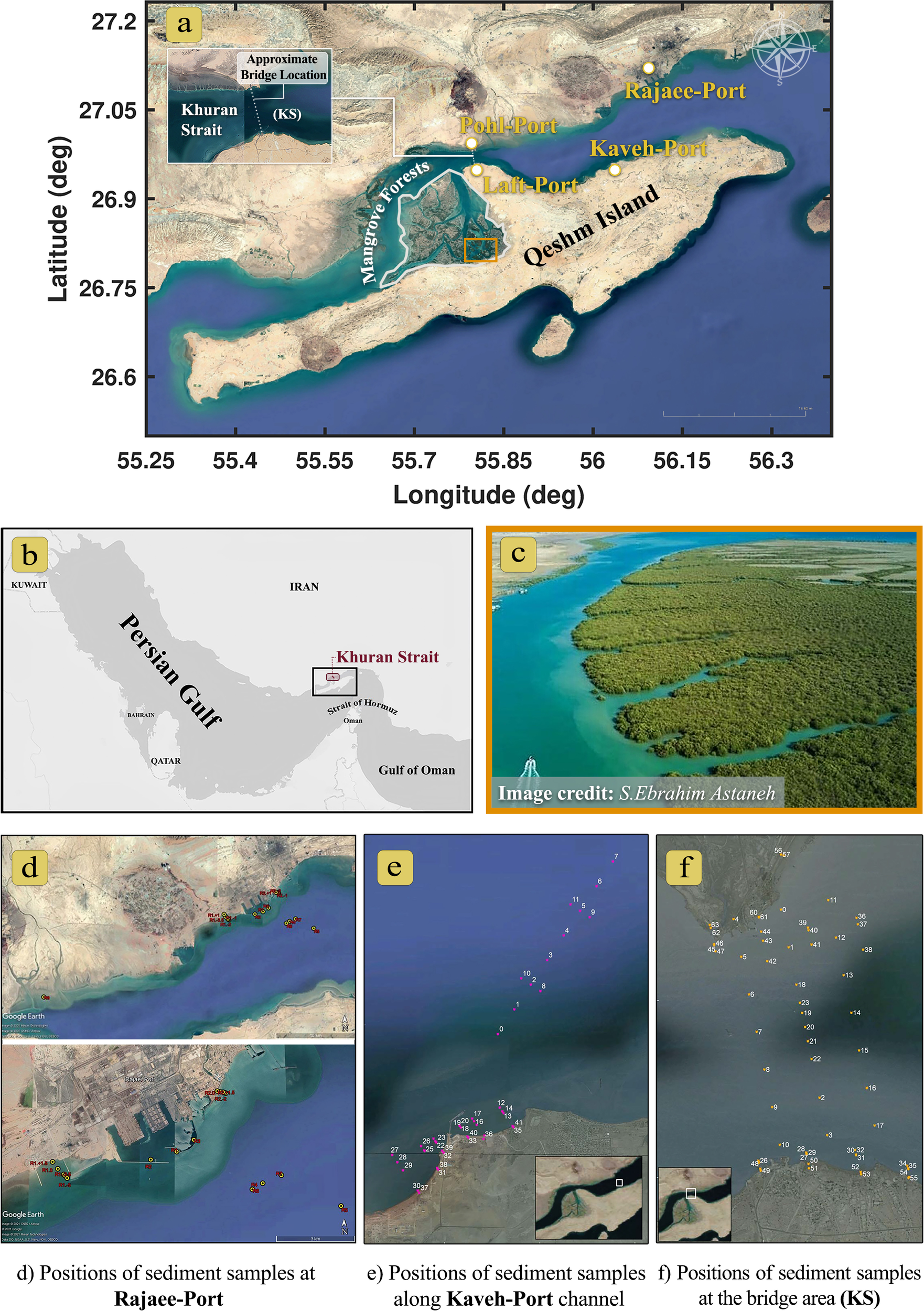
(a, b) The study area is the Khuran Strait, which is located between Qeshm Island and the Iranian mother land at the Strait of Hormuz. (c) The aerial photo shows some part of the extensive mangrove habitat, located on the western part of the strait (image credit: S. Ebrahim Astaneh) The location of sediment samples is shown in the bottom frames: (d) Access channel of Rajaee Port, (e) Access channel of Kaveh Port, and (f) The narrowest part of the KS (the centreline of the probable PG Bridge).
2 Study area
The KS is situated between Qeshm Island and the Iranian mainland, approximately 100 km from the Strait of Hormuz in the PG at coordinates 26°45’N and 55°40’E (Figure 1). The KS extends approximately 110 km in length and has a minimum width of about two km at Pohl Port. The hydrodynamics of this narrow, sheltered area, with a maximum depth of 42 m, are dominated by short-crested, small waves (Jedari Attari et al., 2024) and strong tidal currents reaching up to 1.85 m/s. The prevailing northeast-southwest winds run parallel to the channel (Figure 2). This region experiences semi-diurnal tides, where the tidal range, which can reach nearly 5 m during spring tides, significantly influences the water movement within the strait. The strong ebb and flood currents associated with these tides play a crucial role in shaping the intertidal topography and transporting sediments.
Figure 2
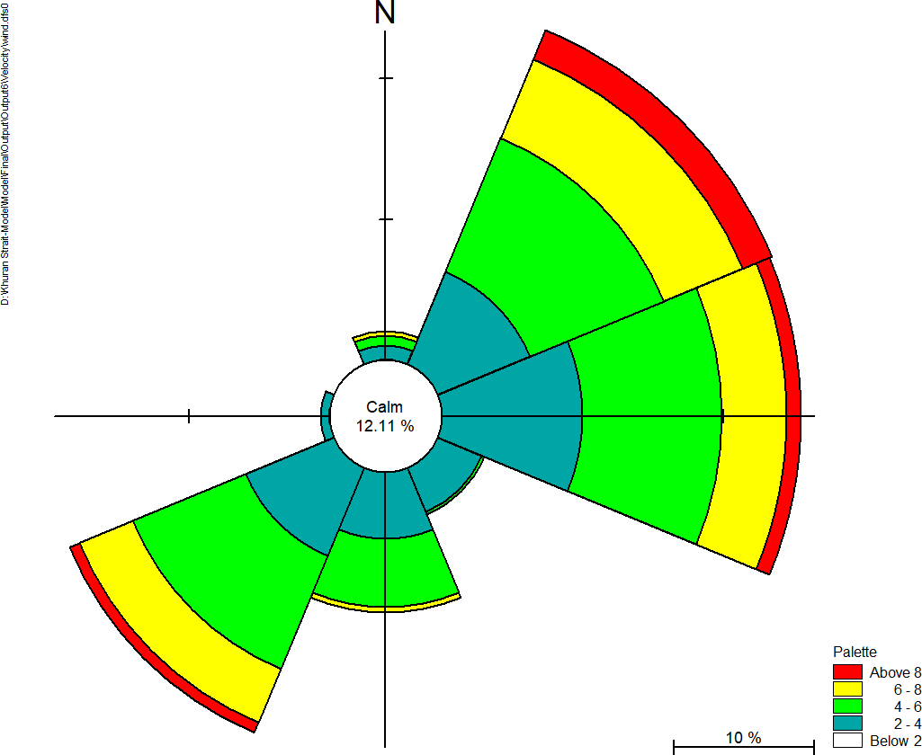
Wind rose at Pohl Station, where the prevailing northeast-southwest winds run parallel to the Khuran Starit channel (DNP (Darya Negar Pars Consulting Engineers), 2013).
The KS is adjacent to the Mangrove forests, primarily composed of Avicennia marina mangroves, on its western side. This ecologically important area supports diverse wildlife, including fish, reptiles, and bird species. The forest is submerged during high tide and re-emerges at low tide, creating waterways that influence the strait’s hydrodynamic patterns.
3 Field measurements
A comprehensive set of field measurements was carried out to study the hydrodynamics and morphodynamics of the study area. The data consists of vertical current profiling, directional waves, water levels, sediment grab samplings, and SSC. Due to the high current speed in the area, data retrieval and redeployment operation of instruments were a significant part of measurement. The features of the stations including instrument depth, coordinates, and measurement periods are presented in Tables 1, 2. All instruments were deployed as bottom-mounted stations. The sampling frequency for wave measurements was set at 2 Hz, while current data were collected every 15, 20 and 30 minutes for the AWAC (Nortek AWAC 1 MHz), SON (SonTek ADP/ADCP 1 MHz) and ARG (SonTek Argonaut – XR 1MHz) instruments, respectively. The RBR (TGR – 1050) water level measurements were provided every 10 minutes. The bin size for all instruments measuring current profiles was 1 m, and the blind zone for AWAC is estimated 0.5 to 1.5 m, while for ARG and SON it ranges from 0.5 to 0.8 m. The number of layers for each instrument was set at 1 m. Quality control for all instruments included monitoring of battery voltage, signal strength, and beam quality to ensure reliability and accuracy of data collection together with a regular bi-weekly to monthly data retrieval.
Table 1
| Station | Code | Instrument (depth, m) | Coordinate UTM R40 | Measurement period | ||
|---|---|---|---|---|---|---|
| X | Y | Start | End | |||
| Bahonar | RBR1 | 18 | 56.2 | 27.15 | 06/01/2013 | 7/22/2013 |
| Qeshm | RBR2 | 12 | 56.27 | 26.96 | 06/03/2013 | 7/22/2013 |
| Kaveh | RBR3 | 13 | 55.98 | 26.94 | 06/03/2013 | 7/22/2013 |
| Pohl | RBR4 | 12 | 55.74 | 26.97 | 5/31/2013 | 7/19/2013 |
| Basaeidu | RBR5 | 13 | 55.27 | 26.66 | 06/01/2013 | 7/22/2013 |
| Berke | RBR6 | 14 | 55.21 | 26.76 | 06/03/2013 | 7/21/2013 |
| Laft | AW2 | 23 | 55.75 | 26.96 | 06/03/2013 | 7/22/2013 |
Field measurements of water level elevation in the KS.
Table 2
| Station | Code | Instrument type | Instrument (depth, m) | Coordinate UTM R40 | Measurement period | ||
|---|---|---|---|---|---|---|---|
| X | Y | Start | End | ||||
| Laft | AW2 | AWAC | 23 | 55.75 | 26.96 | 06/06/2013 | 2013/20/7 |
| Kaveh | SON1 | Mini SonTek | 8 | 55.99 | 26.95 | 2013/13/5 | 2013/27/7 |
Field measurements of current velocity in the KS.
3.1 Bathymetry and hydrographic survey
Bathymetry data was collected from various resources and integrated to achieve maximum accuracy. These sources include the 1-minute gridded regional relief data (ETOPO) from the US National Geophysical Data Center, hydrographic maps (scales 1:100,000 and 1:25,000) from Iran’s National Cartographic Center (NCC Tide), the British Admiralty Nautical Map (Chart 3172), ECRI 2006 coastline survey data, and regional Landsat satellite imagery. For the integration of bathymetric data from various sources, all datasets were standardized to mean sea level. In regions with high-quality data, coarser datasets were excluded. Where no high-resolution data was available, the aforementioned sources were combined. The datasets were blended to ensure consistent vertical alignment and avoid overlapping coverage. Transitions between areas sourced from different datasets were smoothed to ensure seamless integration.
A hydrographic survey was carried out in the middle section of the strait at the proposed location of the PG Bridge (Figure 3). Survey lines extended 500 m on either side of the bridge centerline, with varying sounding intervals. Within the first 200 m from the centerline, soundings were taken every 20 m. This interval increased to 50 m for the next 400 m and to 100 m for the remaining distance. Additionally, perpendicular check lines were surveyed every 200 m (DNP (Darya Negar Pars Consulting Engineers), 2013). Figure 3 illustrates that the middle section of the KS is covered by sand dunes, with rocks and an electricity pylon also indicated. Sand dunes are approximately 2 to 6 m high with a wavelength of 100 to 150 m. Direct observations confirmed the mobility of these sand dunes, making their dynamics a primary focus of this study (DNP (Darya Negar Pars Consulting Engineers), 2013).
Figure 3
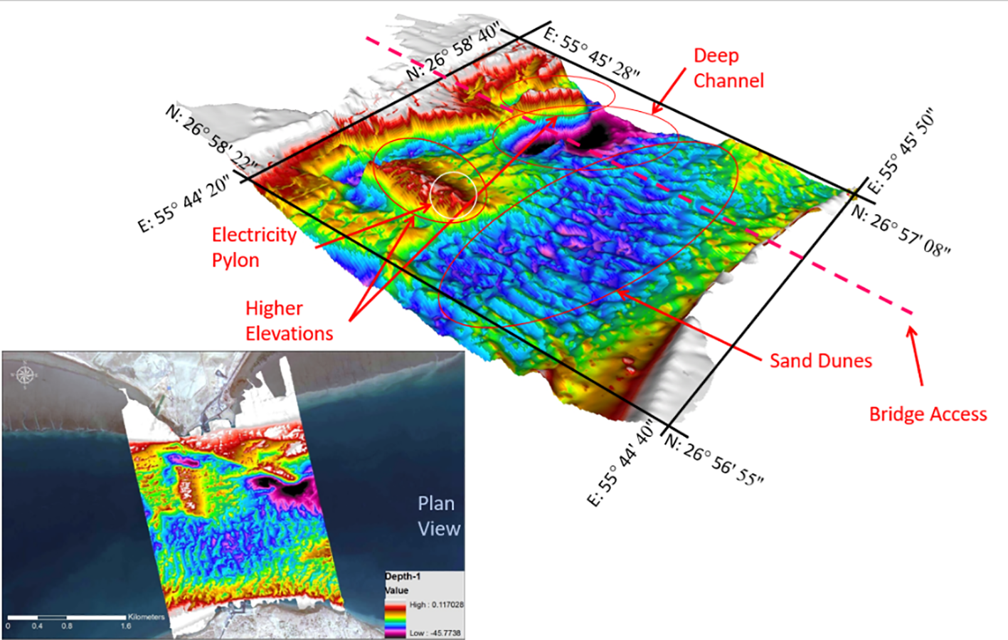
Hydrographic survey data in the middle of the KS. Dynamic sand dune fields can be observed in the southern part of the strait, which are approximately 2~6 m high and have a wavelength of approximately 100~150 m.
3.2 Wave and current measurements
Water levels were measured at six tide stations using RBR instruments (Richard Brancker Research) (Figure 4a), which RBR1 to RBR6 are located at Bahonar, Qeshm, Kaveh, Pohl, Berke and Basaeidu, respectively. Current profiling and wave data were collected at two stations using ADCP (Acoustic Doppler Current Profiler) instruments. One ADCP was deployed at the western boundary to record offshore waves from the PG through the Strait of Hormuz (SON2), while the other one was placed in shallow waters near Kaveh Port (SON1). The dominant waves on the eastern side of the KS are primarily short-period wind-driven seas, coming from the southwest, with minimal penetration to the middle part of the KS. These waves typically average 0.5 m of height, rarely exceeding 1 m. Offshore waves were recorded using a Nortek AWAC 1000 kHz, equipped with an AST (Acoustic Surface Track) sensor, capable of tracking the water surface from the seabed at the eastern boundary (AW1) and at the middle of strait (AW2). This system detected wave periods as short as 4s. A SonTek ADCP 1000 kHz was deployed in a nearshore area, capable of measuring currents at all depths due to its acoustic power (Figure 4b). Given the 4 to 6 second wave period in the PG, wave measurements were practical within a 5 to 8 m depth for these instruments. The maximum recorded wave height in the middle part of the KS was approximately 0.75 m with a 4-second period (Haghshenas et al., 2014). Figures 4c-e demonstrate locations of tide gauges adapted for calibration and validation of the regional model results, borehole locations in the middle of the KS, and locations of conducted sediment samplings, respectively.
Figure 4
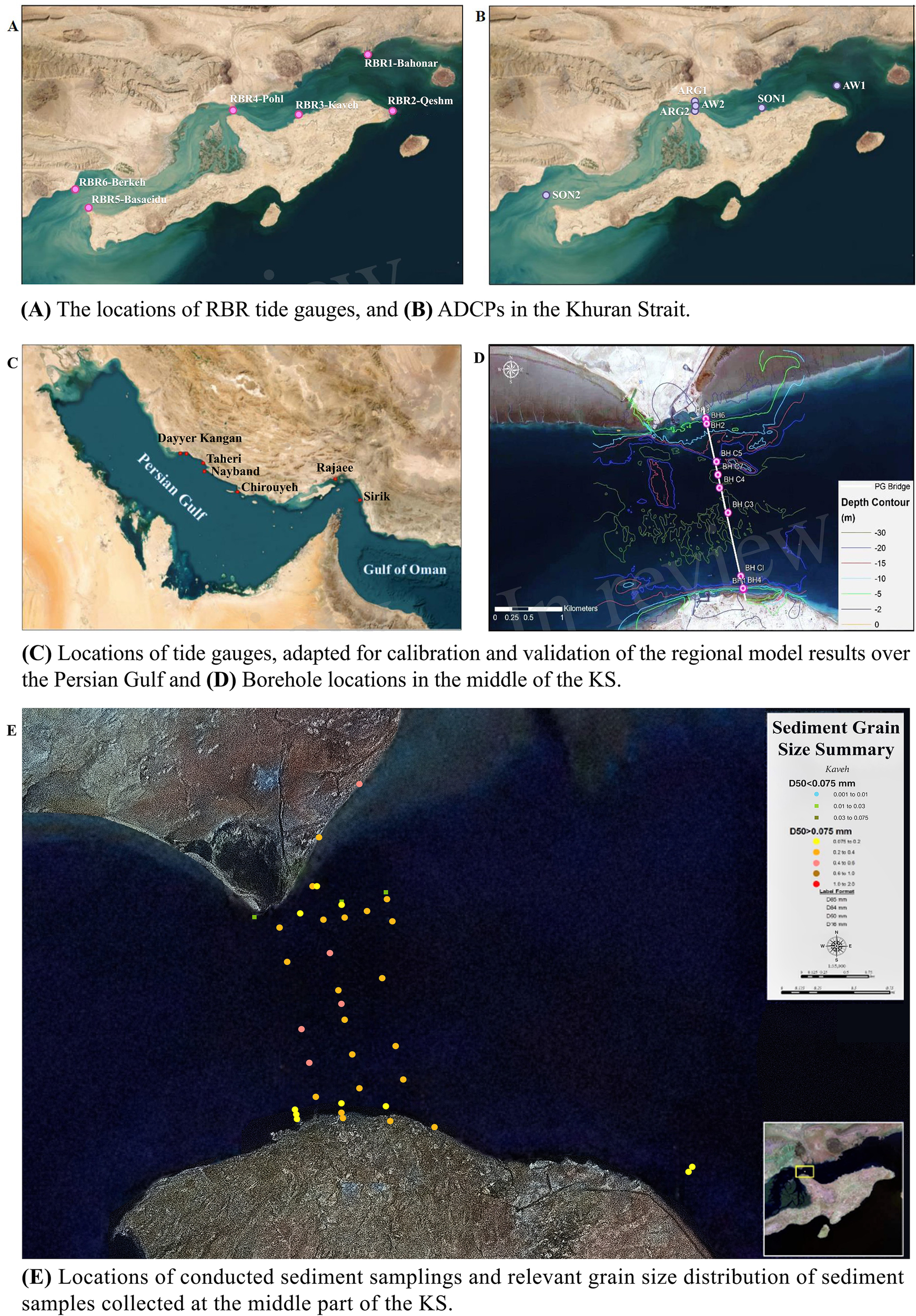
(a) The locations of RBR tide gauges, and (b) deployed ADCPs in the KS, (c) locations of tide gauges, adapted for calibration and validation of the regional model results over the Persian Gulf, (d) borehole locations in the middle of the KS, and (e) locations of conducted sediment samplings and relevant grain size distribution of sediment samples collected at the middle part of the KS.
3.3 Sediment sampling and geotechnical investigations
Figure 4e illustrates the locations of sediment samples collected in the central region of the KS. Disturbed samples were collected using a Van Veen grab sampler. The distribution of the particle sizes larger than 75 μm (remaining on Sieve No. 200) was determined by sieving, while the distribution of particle sizes smaller than 75 μm (passing through Sieve No. 200) was determined by the sedimentation process and using a hydrometer. Samples were collected at the following locations (DNP (Darya Negar Pars Consulting Engineers), 2013; MEWE (Middle East Water and Environment), 2021):
-
The narrowest part of the KS (the centreline of the probable PG Bridge).
-
250 m and 750 m from either side of the centreline.
-
Access channel of Kaveh Port.
-
Access channel of Rajaee Port.
The median grain size () of collected samples at the middle part of the KS are presented in Figure 4e. is reported 0.23 mm for the access channel of Kaveh Port. Grain size analysis of surface sediment samples indicates a D50 of approximately 0.5 mm in the sand dune area; while typical median grain size of sand dune sediment in tidal flow is 0.3~0.6 mm. Three samples were collected for Rajaee Port navigation channel, over a cross section of the access channel. The percentage of sediments finer than 75 μm is estimated to be 58% with a of 0.06 mm for the sample taken from the middle of the channel. Relevant values for these two parameters for the samples taken from the western and eastern sides of the navigation channel is estimated 15% - 0.15 mm and 53% - 0.05 mm, respectively. Figure 4d shows the location of boreholes along the centerline of the PG Bridge in the middle of the KS, including the borehole log for Borehole C3 drilled within the trough between two sand dunes in the southern part of the central KS, each approximately 3 to 4 m high. The bore log from Borehole C3, shown in Figure 5, demonstrates the soil stratification and indicates that the seabed is covered by ~1.5 m of fine to medium sand, over an approximately 0.5 m thick layer of soft to firm clay. The sand layer on the seabed has considerable thickness on top of a hard clay layer, moving under the current action and any bridge pier constructed in this zone is expected to cause seabed scour.
Figure 5
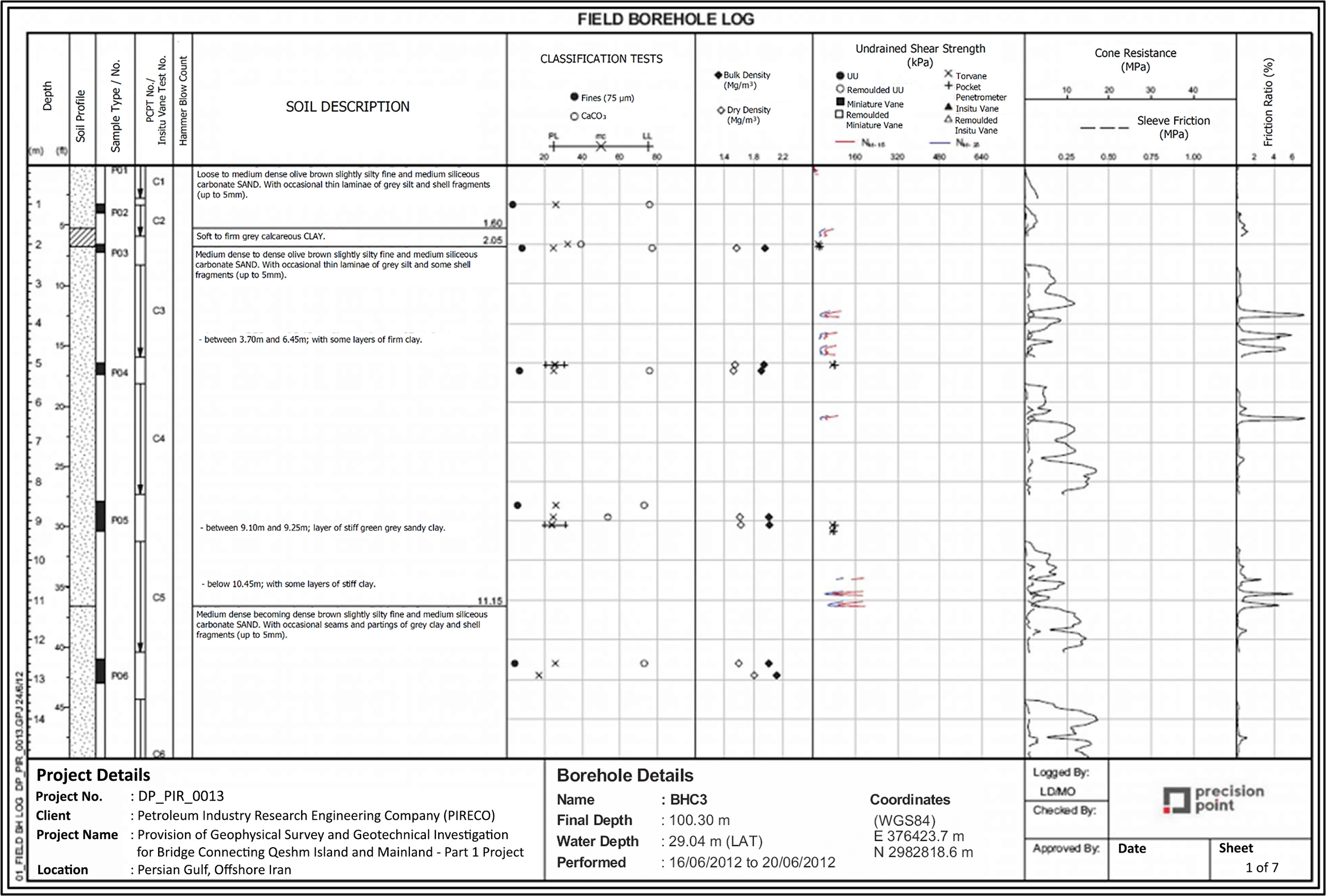
Bore log and geotechnical analysis of soil stratification for Borehole C3, located on the sand dune field.
4 Numerical modelling
Delft3D, an integrated open-source software developed by Deltares, was used for numerical modeling in this study. The software simulates flows, waves, sediment transport, water quality, and morphological changes. Delft3D-FLOW, a component of Delft3D, solves the Navier-Stokes equations for incompressible flow on an orthogonal curvilinear grid using finite difference methods (Deltares, 2021). In general, the model applies the shallow water approximation and can operate in both 2D depth-averaged and 3D baroclinic modes, making it well-suited for simulating hydrodynamics in coastal, estuarine, and riverine systems. It uses a staggered grid layout and employs an implicit or semi-implicit time-stepping scheme to ensure numerical stability. As a finite difference model, it computes fluxes directly at cell faces without using control volumes, which distinguishes it from finite volume models and contributes to its computational efficiency on structured grids. The sediment transport module in Delft3D computes sediment movement using empirical and semi-empirical transport formulas, such as those by Van Rijn or Engelund-Hansen, depending on sediment type and flow conditions (Van Rijn, 2001; Engelund and Hansen, 1967; Jedari Attari, 2025). In this study, the Van Rijn formula was specifically applied to calculate both bedload and suspended load transport. These formulations link flow velocity and bed shear stress to sediment transport rates, while the model dynamically updates bed elevation using a mass-balance approach.
4.1 Regional and local models
A regional model was configured to simulate tidal currents in the PG. The PG, extending approximately 1000 km between latitudes 24°N and 30°N and longitudes 48°E and 56°E, has a maximum width of about 290 km at its center. The PG reaches its maximum depth of 110 m in the Strait of Hormuz, which connects it to the Gulf of Oman.
To minimize boundary effects, the open boundary of the enclosed regional model was positioned far from the study area. Precise water levels were imposed along two-line boundaries in the western Gulf of Oman: (1) connecting Jask and Dibba Beach (BND1), and (2) connecting Jask and Almasnaeh (BND2) (Figure 6). Model outputs were compared to measurements to determine the optimal location.
Figure 6
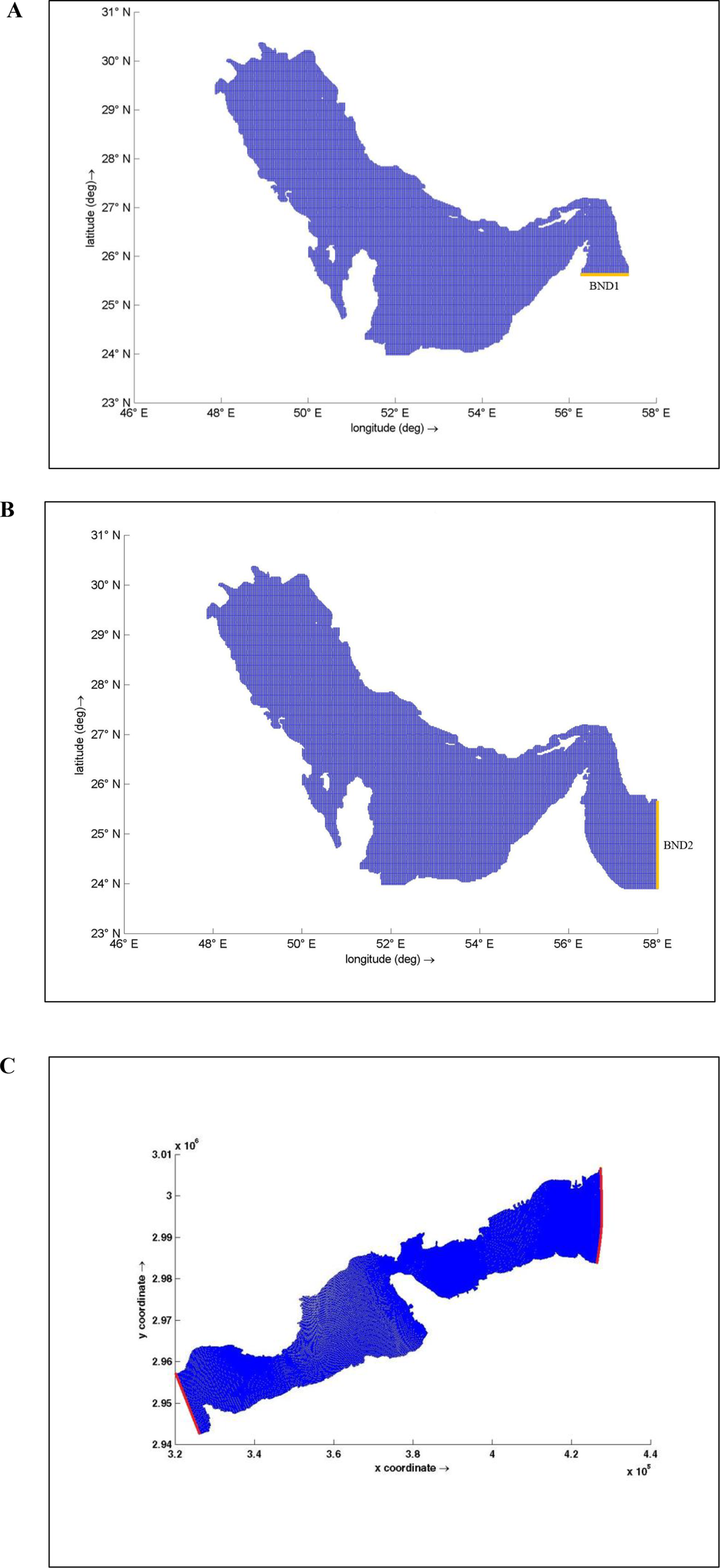
Computational grid for the Persian Gulf and the Strait of Hormuz (0.02°) and the open boundary alternatives: (A) BND1, (B) BND2, (C) Computational domain and adopted simulation grid for the local model. The open boundaries are shown with two red lines.
The regional model employs a regular grid with a 0.01° resolution on an orthogonal curvilinear spherical coordinate system, resulting in 141,248 nodes. The water level boundary condition was dynamically forced using TPXO8.0. Surface elevations at the open boundary were derived from this model, incorporating 13 tidal constituents: M2, S2, N2, K2, K1, O1, P1, Q1, M4, MS4, MN4, MM, and MF.
To enhance precision, accuracy, and computational efficiency, a local model was developed for the study area, complementing the larger-scale model. The model was employed to simulate hydrodynamic forces, characterize seabed parameters, and analyze sediment transport within the KS to investigate the feasibility of sand dune dynamics and sediment transport patterns. The model utilizes a Cartesian coordinate system with curvilinear grids generated by the Delft3D-RGFGRID module (Figure 6). The grid spacing near the boundaries was set at 279 m, narrowing to 19 m in certain areas, with spacing gradually increasing towards the boundaries.
The water level elevations at open boundaries of the local model were obtained from the larger-scale regional model. The eastern model boundary extended from Bahonar to Qeshm, while the western boundary stretched from Berke to Basaeidu (Figure 6). This configuration enabled tidal current modeling with a 60-second time step. Physical parameters were input into Delft3D-Flow for the hydrodynamic model, enabling the simulation of sediment transport in the study area. The turbulent flow generates bed shear stress for the 2D depth-averaged flow, which can be represented by a quadratic friction law (Equation 1) as follows (Whipple, 2019):
where, represents the depth-averaged horizontal velocity magnitude, which is crucial for characterizing the flow intensity, U is the local flow velocity, is the reference fluid density, important for computing momentum and buoyancy forces, is gravitational acceleration, which drives pressure gradients in free-surface flows, and denotes the 2D Chezy coefficient, the key parameter reflecting bed roughness and resistance to flow.
4.2 Model calibration and validation
Statistical parameters including root mean square error (RMSE), correlation coefficient (R), coefficient of determination (R²), index of agreement (d) and standard deviation (σ) as indicated in Equation 6 were used to evaluate the models’ performance at specified stations.
where, and n represent the water elevation of model, observed water level and the number of samples, respectively.
Simulated water levels from the regional model were compared to available 10-minute interval data at 7 monitoring stations from 2009 (Figure 4c) to assess sensitivity to grid size, Manning coefficient, and open boundary location. Table 3 presents statistical parameters comparing model outputs to field measurements for different open boundary location (Figure 6). Results indicate that the Jask-Almasnaeh boundary (BND2) produced better model performance compared to the Jask-Dibba Beach boundary (BND1). Table 4 compares the performance of simulated water levels for grid resolutions of 0.01° and 0.02°, demonstrating the superiority of the 0.01° resolution. The sensitivity analysis indicated no need for more grid refinement. By comparing model outputs for different Manning coefficients (n = 0.01, 0.02, 0.022, 0.025, and 0.03), an optimal value of 0.022 s was selected (Table 5).
Table 3
| Station Open boundary | RMSE (m) | R | R 2 | d | ||||
|---|---|---|---|---|---|---|---|---|
| BND1 | BND2 | BND1 | BND2 | BND1 | BND2 | BND1 | BND2 | |
| Chirouyeh | 0.17 | 0.15 | 0.93 | 0.95 | 0.8 | 0.90 | 0.98 | 0.99 |
| Dayyer | 0.15 | 0.16 | 0.96 | 0.96 | 0.93 | 0.92 | 0.97 | 0.97 |
| Kangan | 0.14 | 0.14 | 0.97 | 0.97 | 0.95 | 0.95 | 0.97 | 0.97 |
| Nayband | 0.10 | 0.04 | 0.96 | 0.98 | 0.91 | 0.95 | 0.96 | 0.98 |
| Rajaee | 0.15 | 0.14 | 0.99 | 0.99 | 0.98 | 0.98 | 0.99 | 0.99 |
| Sirik | 0.10 | 0.09 | 0.99 | 0.99 | 0.98 | 0.98 | 0.99 | 0.99 |
| Taheri | 0.13 | 0.15 | 0.97 | 0.96 | 0.91 | 0.93 | 0.97 | 0.96 |
Evaluation metrics for regional model at different open boundary locations in the PG.
Table 4
| Station Grid size | RMSE (m) | R | R 2 | d | ||||
|---|---|---|---|---|---|---|---|---|
| 0.01° | 0.02° | 0.01° | 0.02° | 0.01° | 0.02° | 0.01° | 0.02° | |
| Chirouyeh | 0.15 | 0.44 | 0.95 | 0.42 | 0.90 | 0.35 | 0.98 | 0.41 |
| Dayyer | 0.16 | 0.40 | 0.96 | 0.52 | 0.92 | 0.38 | 0.96 | 0.49 |
| Kangan | 0.14 | 0.32 | 0.97 | 0.76 | 0.95 | 0.58 | 0.97 | 0.82 |
| Nayband | 0.04 | 0. 35 | 0.98 | 0.54 | 0.95 | 0.40 | 0.98 | 0.52 |
| Rajaee | 0.14 | 0.20 | 0.99 | 0.72 | 0.98 | 0.69 | 0.99 | 0.60 |
| Sirik | 0.09 | 0.25 | 0.99 | 0.66 | 0.98 | 0.60 | 0.99 | 0.62 |
| Taheri | 0.15 | 0.38 | 0.97 | 0.56 | 0.93 | 0.37 | 0.97 | 0.65 |
Evaluation metrics for regional model and field measurements using different grid size.
Table 5
| Statistical parameter | Manning coefficient | Chirouyeh | Dyyer | Kangan | Nayband | Rajaee | Sirik | Taheri |
|---|---|---|---|---|---|---|---|---|
|
RMSE
(m) |
n = 0.01 | 0.28 | 0.34 | 0.30 | 0.33 | 0.29 | 0.27 | 0.34 |
| n = 0.02 | 0.22 | 0.33 | 0.25 | 0.29 | 0.26 | 0.26 | 0.30 | |
| n = 0.03 | 0.17 | 0.18 | 0.25 | 0.28 | 0.27 | 026 | 0.30 | |
| n = 0.022 | 0.15 | 0.16 | 0.14 | 0.04 | 0.14 | 0.09 | 0.14 | |
| R | n = 0.01 | 084 | 0.92 | 0.93 | 0.86 | 0.98 | 0.98 | 0.86 |
| n = 0.02 | 0.95 | 0.95 | 0.96 | 0.95 | 0.99 | 0.99 | 0.94 | |
| n = 0.03 | 0.97 | 0.93 | 0.96 | 0.97 | 0.99 | 0.99 | 0.96 | |
| n = 0.022 | 0.95 | 0.96 | 0.97 | 0.98 | 0.99 | 0.99 | 0.96 | |
| R 2 | n = 0.01 | 0.71 | 0.85 | 0.90 | 0.73 | 0.96 | 0.97 | 0.94 |
| n = 0.02 | 0.90 | 0.90 | 0.92 | 0.90 | 0.98 | 0.99 | 0.96 | |
| n = 0.03 | 0.93 | 0.87 | 0.95 | 0.94 | 0.98 | 0.98 | 0.96 | |
| n = 0.022 | 0.90 | 0.92 | 0.95 | 0.95 | 0.98 | 0.98 | 0.93 | |
| d | n = 0.01 | 0.97 | 0.84 | 0.80 | 0.80 | 0.97 | 0.97 | 0.81 |
| n = 0.02 | 0.98 | 0.82 | 0.80 | 0.83 | 0.98 | 0.98 | 0.82 | |
| n = 0.03 | 0.99 | 0.79 | 0.80 | 0.82 | 0.96 | 0.96 | 0.81 | |
| n = 0.022 | 0.99 | 0.97 | 0.97 | 0.98 | 0.99 | 0.99 | 0.97 |
Regional model calibration statistics for varying Manning coefficients in the PG.
4.3 Sediment transport and morphodynamic models
Predicting bathymetric changes in the protected areas of the KS in the northern Qeshm Island is essential. Additionally, assessing the potential for erosion and deposition around any probable infrastructure is essential. In muddy areas where wave action is minimal, tidal currents are the primary drivers of morphological changes (Bird, 2008). The complex topography of the KS, being open at both ends, is significantly influenced by tidal currents during ebb and flood phases.
Previous studies of the KS suggest that the channel primarily consists of fine, cohesive sediment, with less than 5% clay, as determined by sample analysis (DNP (Darya Negar Pars Consulting Engineers), 2013). The eastern part of the channel exhibits a finer grain size distribution, and it is predominantly covered by silt. Although the sand content in the KS is little (<10%), field data shows that the narrowest part of the channel contains 75% coarse-grained sediments and 25% fine-grained ones. Surface sediment samples in the sand dune area have a median grain size of approximately 0.3 mm (Figure 4e), which aligns with the typical range of 0.3 to 0.6 mm for sand dune sediments in tidal flows based on general observations. Sediment classes in the model were categorized as either fine sediments, comprising both silt and mud, or sand with a median grain size of 0.3 mm.
While numerical models often separate coarse and fine sediment transport, this study employs a mixed sand-mud model within Delft3D to simulate sediment transport rates, considering the complex interplay between coarse and fine particles. The 2D depth-averaged coupled hydrodynamic and sediment transport model can be used to study sediment transport processes in the KS and the dynamics of sand dunes in its central region. Delft3D categorizes sediments into bedload transport and suspended load transport. Cohesive sediments (muds, ≤ 63 µm) are defined as suspended sediments, while non-cohesive sediments (sands, >63 µm) can be either suspended or bedload (Van Rijn, 1993). The transport of cohesive sediments is computed based on the Partheniades-Krone formulations (Partheniades, 1965).
Three-dimensional transport of suspended load is obtained by solving three-dimensional advection-diffusion equations (Equation 7), described as (Van Rijn, 1993):
where represents the mass concentration of sediment particle I, , u,v and w are flow velocity components in three directions, ; are eddy diffusivities of sediment particle of I in direction of x, y, z, respectively, and defines settling velocity of particle I, .
Richardson and Zaki (1954) introduced distinct formulations for the settling velocities (Equation 8) of sand and mud at high concentrations. Delft3D assumes a constant fall velocity for cohesive models, with the sediment fraction falling at a rate of 2.5 mm/s in the channel (Richardson and Zaki, 1954).
where is the settling velocity for sand and mud fraction, is the basic sediment fraction specific settling velocity, is the reference density, and is the sum of the mass concentration of the sediment fractions.
In the absence of effective waves, the simulation of the bed load magnitude is carried out with Van Rijn (1993) formulation (Equation 9), using the updated coefficients after Van Rijn et al. (2000, 2003).
where represents the total bedload transport rate, and is non-dimensional bed-shear stress, and is non-dimensional particle diameter, and , where is the effective bed-shear velocity () and is the efficiency factor for currents, defined as the ratio between gain related friction factor and total current-related friction factor.
At the eastern boundary, a uniform SSC of 0.06 kg/m³ was applied, while at the western boundary, the SSC was set to 0.03 kg/m³. This adjustment reflects the higher rate of SSC observed at the eastern boundary during model calibration. Additionally, a Thatcher-Harleman time lag of 120 minutes was incorporated into the model. The erosion parameter (M) () was set to calculate erosion and deposition fluxes of cohesive sediment fractions by Partheniades-Krone’s formula (Equation 10) (Partheniades, 1965):
where, is the maximum bed shear stress due to the current and wave and shows critical shear stress for erosion. Deposition flux (D) represents flux of sedimentation at bed level related to critical deposition shear stress () (Equation 11), C is sediment concentration () and is the settling velocity of cohesive sediment fraction which is derived from following formulation (Equation 12) of Richardson-Zaki in which is fall velocity of fractions in clear water and volumetric sediment concentration of .
5 Results
The Results section is organized into three parts; model validation, dynamic flow and sediment processes, and sedimentation/erosion patterns. The hydrodynamics and sediment transport models were carried out for the period of the study, as described in Section 4, and relevant results are presented in this section. The validation of the regional model was conducted over a month, from August 9, 2009, to September 9, 2009. Comparing the time series and scatter plots of simulated water levels with observations, Figures 7, 8 demonstrates that the model performs well in accurately replicating water levels in the PG. All stations achieved similar performance based on RMSE comparisons. The correlation coefficients and coefficient of determination indicate a strong fit between the predicted parameters and the measurements. It can be concluded that the regional model outputs are reliable for use in local modeling of the KS. Statistical parameters (Equations 2-5) were used to calibrate and validate the local model against measured water levels and depth-averaged velocities from early February to early August 2013. The Manning coefficient of 0.022 m−1/3 s was also selected for the local model, consistent with that of the regional model. Figures 9, 10 shows time series and scatter plots comparing simulated and observed water levels in the KS. Figure 11 presents time series and scatter plots comparing simulated and observed depth-averaged velocities at Laft and Kaveh stations in the KS. Tables 6, 7 present statistical parameters comparing simulated and observed water levels and depth-averaged velocities, respectively. It is observed that the local model demonstrates acceptable performance, considering the generally lower accuracy of simulated current speeds compared to water levels in 2D hydrodynamic models.
Figure 7
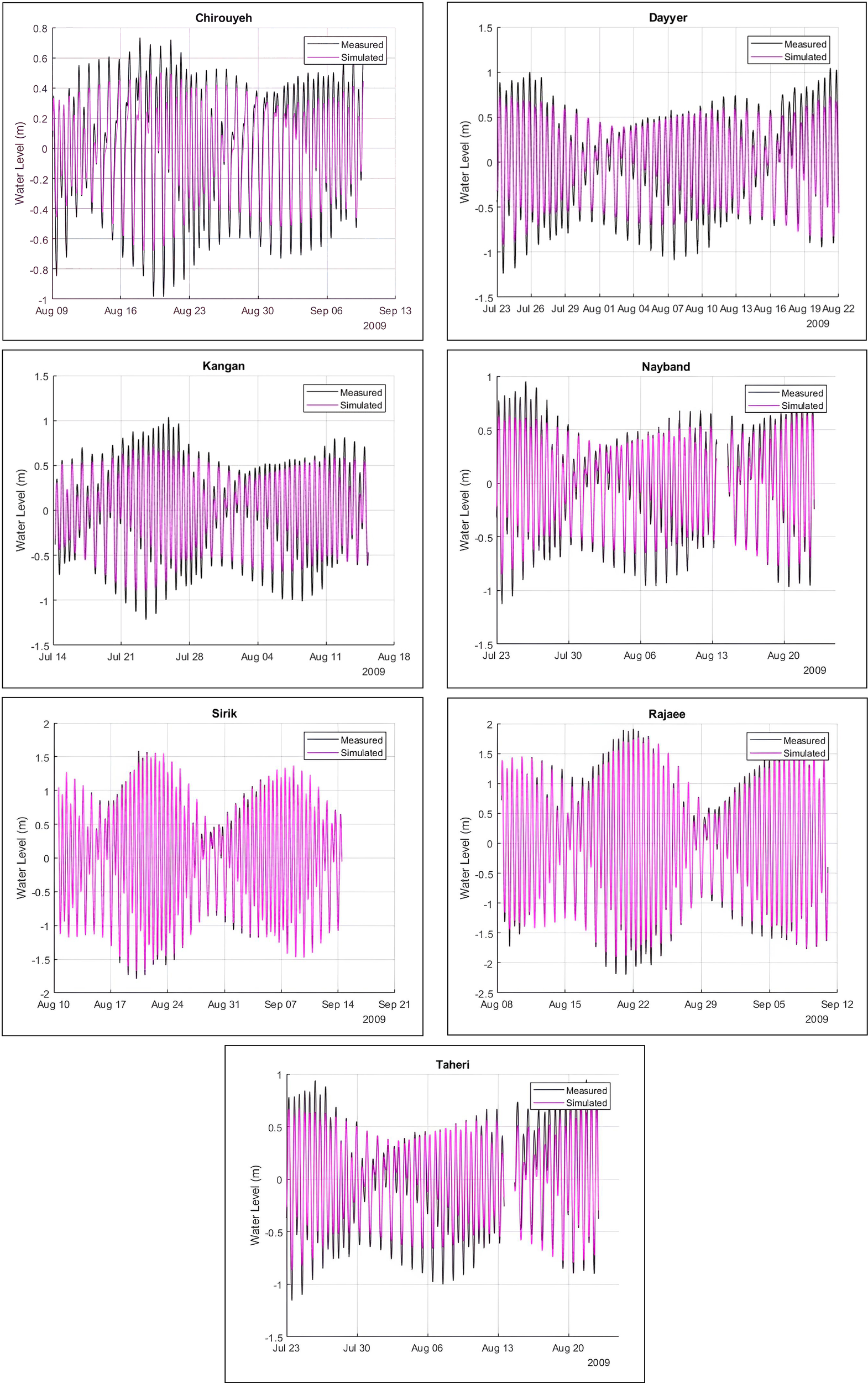
Time series of simulated and observed water levels at seven PG stations.
Figure 8
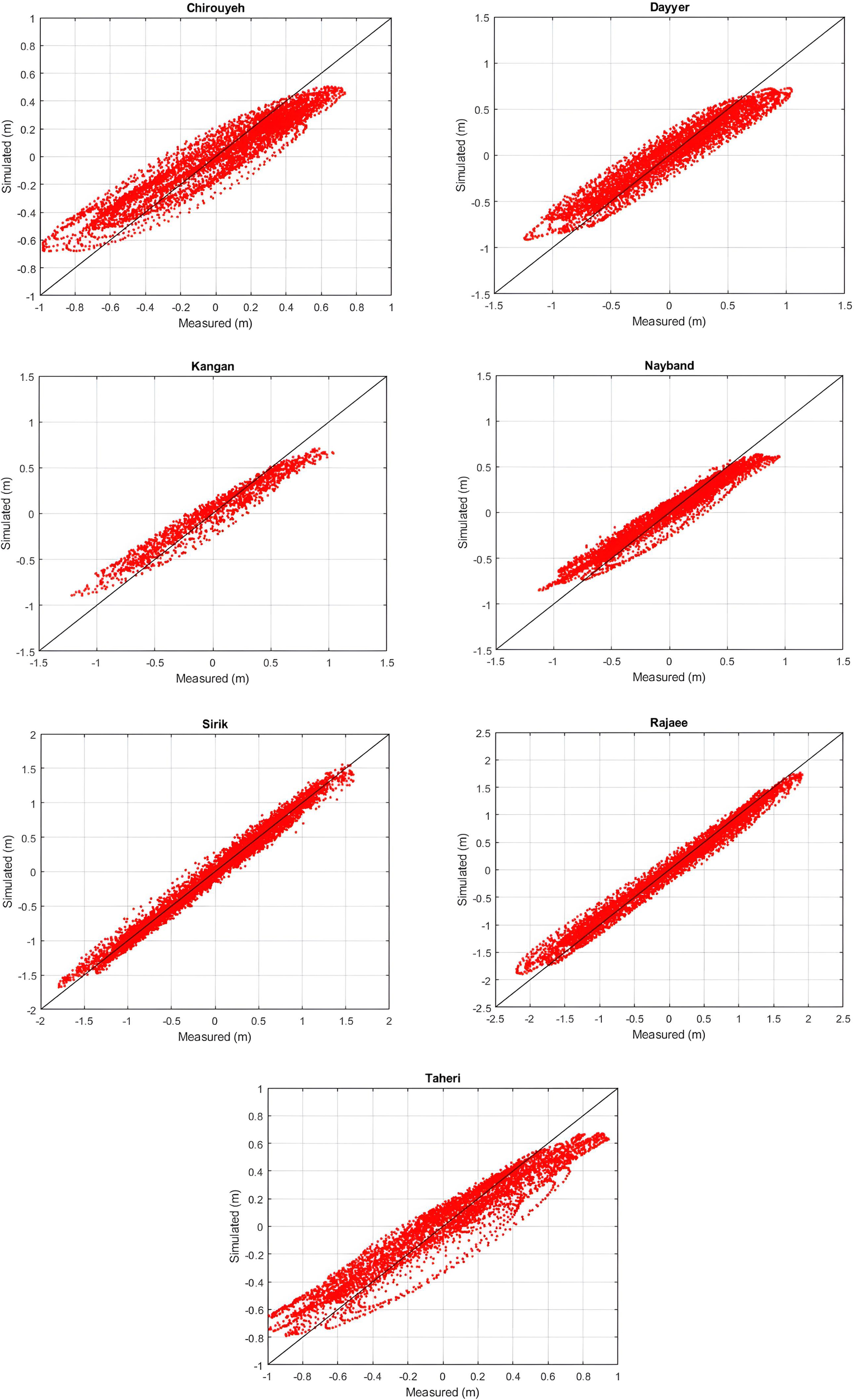
Scatter plots for comparing the simulated water levels by the regional model with the measured levels at the seven observational stations in the PG.
Figure 9
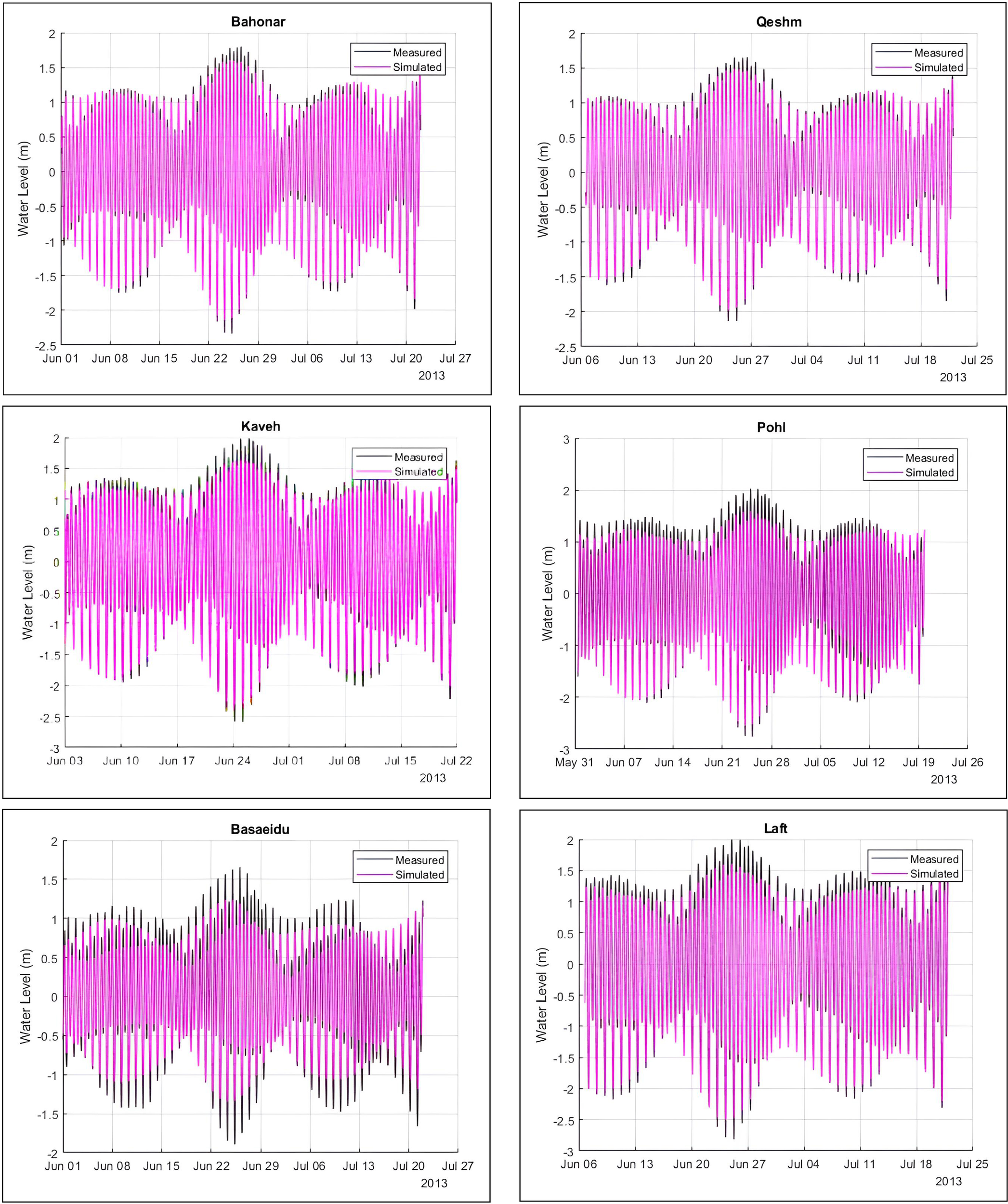
Time series of simulated and observed water levels at in the KS.
Figure 10
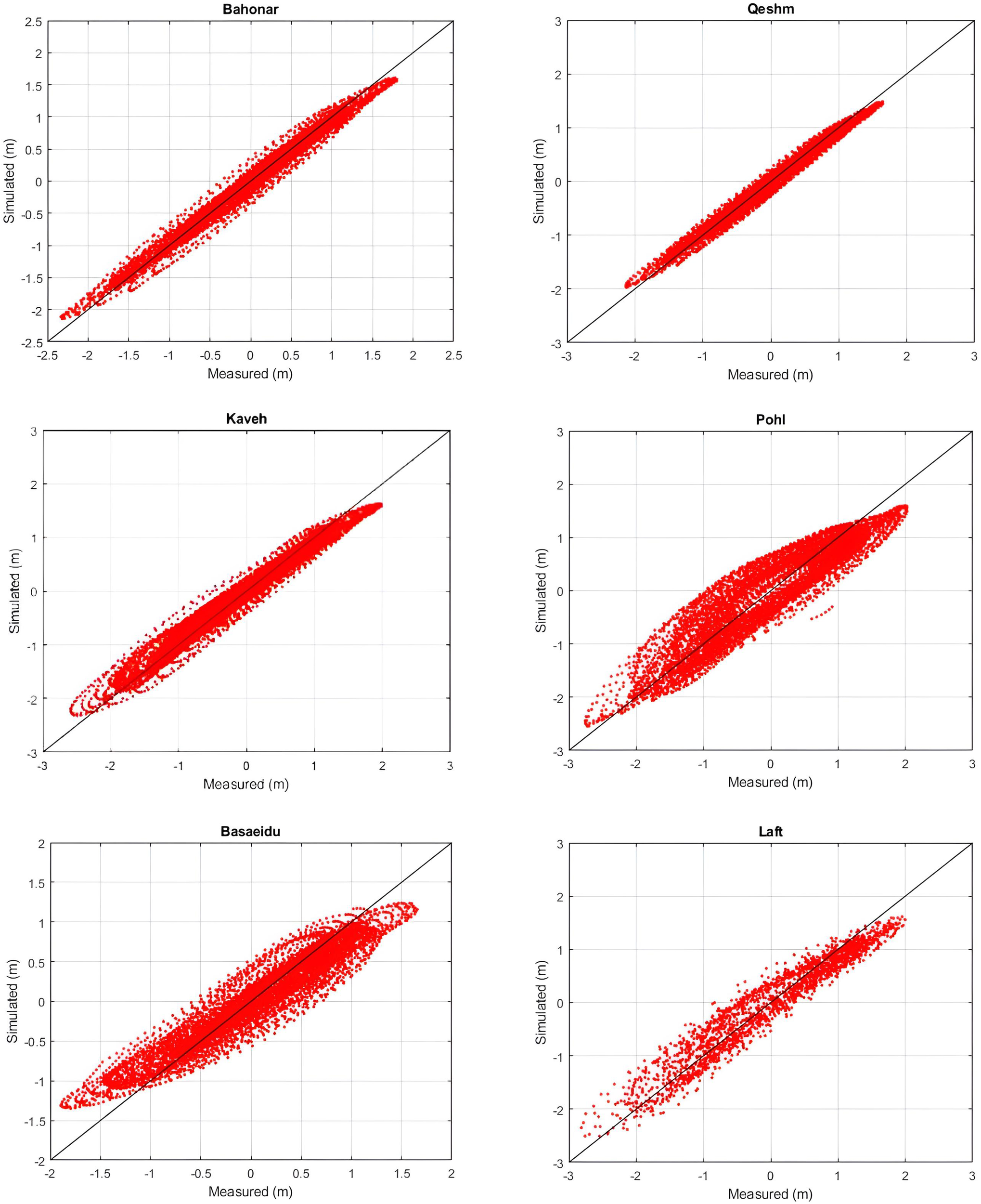
Scatter plots for comparing the simulated water levels by the local model with the measured levels at the six observational stations in the KS.
Figure 11
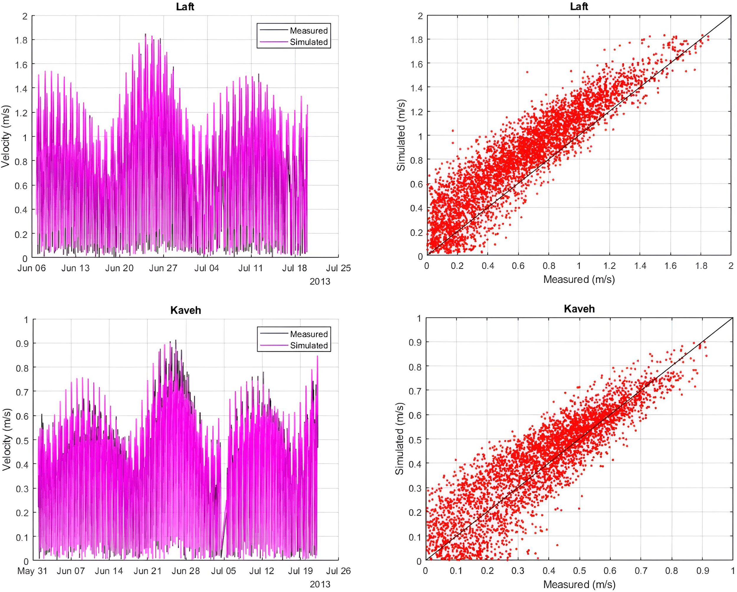
Time series (left) and scatter plots (right) for comparing the simulated depth-averaged current velocities with observational values in Laft and Kaveh Stations.
Table 6
| Station | RMSE (m) | R | R 2 | d | σ |
|---|---|---|---|---|---|
| Bahonar | 0.11 | 0.99 | 0.99 | 0.99 | %0.1 |
| Qeshm | 0.09 | 0.99 | 0.99 | 0.99 | %0.1 |
| Kaveh | 0.17 | 0.99 | 0.97 | 0.99 | %0.2 |
| Pohl | 0.14 | 0.93 | 0.86 | 0.96 | %0.4 |
| Basaeidu | 0.22 | 0.95 | 0.90 | 0.96 | %0.3 |
| Laft | 0.18 | 0.96 | 0.93 | 0.98 | %0.6 |
Calibration statistics for local model and field measurements by using water level elevation.
Table 7
| Station | RMSE (m/s) | R | R 2 | d | σ |
|---|---|---|---|---|---|
| Laft | 0.18 | 0.92 | 0.84 | 0.93 | %0.4 |
| Kaveh | 0.07 | 0.88 | 0.78 | 0.96 | %0.2 |
Calibration statistics for local model and field measurements by using depth-averaged velocity.
Considering the dynamic flow and sediment processes, planar maps of simulated depth-averaged velocity (Figure 12) clearly demonstrate regional variations in dynamic processes during spring and neap tidal cycles. The largest velocities are observed within the main channel and at critical strait entrances during spring tide, while neap tide conditions yield reduced but similar spatial patterns. These results confirm that tidal currents are the dominant force controlling suspended sediment distributions and the overall sedimentary environment in the KS.
Figure 12
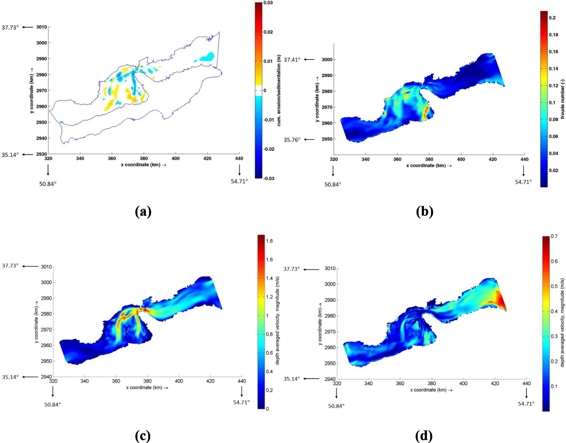
(a) Distribution of erosion and sedimentation over a one-month simulation period, (b) variation of the Froude number over the local model domain in the KS period, (c) 2D distribution of maximum depth-averaged flow velocity magnitude (m/s) in the KS during spring tide event of May 29th, 2013, and (d) 2D distribution of maximum depth-averaged flow velocity magnitude (m/s) in the KS during neap tide event of May 23rd, 2013.
Investigating sedimentation/erosion patterns, the sediment transport model was calibrated based on the observed sedimentation rate at Rajaee Port’s access channel (Figure 1), assuming a normal distribution of cohesive sediment within the channel. Hydrographic surveys conducted from 2008 to 2010 and from 2010 to 2011 reported annual sedimentation rates of 94,000 m³/year and 168,000 m³/year at the access channel, respectively. Table 8 provides the input data for the cohesive sediment model. The sediment concentration at the western boundary was set to 0.03 kg/m3. In contrast, a higher sediment concentration of 0.06 kg/m³ was considered at the eastern boundary. These values are consistent with the suggested input SSCs from Hoseini Chavooshi and Kamalian (2024), which incorporate a range of 0.02 kg/m³ (maximum SSC during neap tide) to 0.08 kg/m³ (maximum SSC during spring tide) as input parameters. The sand-mud mixture model was run for 1 month. Figure 12 presents the results of one-month erosion and sedimentation modeling in the KS. Given the access channel’s dimensions (5500 m long, 200 m wide), the estimated monthly siltation rate is approximately 11,000 m3, resulting in an annual sedimentation of 132,000 m3. This is in a reasonable agreement with reported rates from conducted hydrographic surveys at the access channel from 2008 to 2010. The observed severe erosion in the middle section is attributed to the high velocity of tidal currents, reaching up to 1.85 m/s. The output time series indicate the back-and-forth movement of sand particles, with an average transport rate of approximately 2.5× . The modeled monthly sediment transport rate for sand-mud is 13500 / in the southern part of the channel. The mobility of sand dunes is also supported by the observations during field measurements. The burial of the ARG2 instrument and the rapid decline in data quality shortly after deployment indicate that the sand dunes in the study area are actively shifting and migrating, periodically burying the equipment.
Table 8
| Model parameters | Value | Unit |
|---|---|---|
| Water level | 1 | m |
| Time step | 1 | min |
| Initial sediment layer thickness at bed | 1.6 | m |
| Manning coefficient for hydrodynamic roughness | 0.022 | |
| Dry bed density | 1300 | |
| Settling velocity | 2.5 | mm/s |
| Critical bed shear stress for sedimentation | 0.15 | |
| Critical bed shear stress for erosion | 0.30 | |
| Erosion parameter | 0.00001 | – |
Simulation parameters for cohesive sediment model.
6 Discussions
The hydrodynamics of the KS is driven by strong tidal currents, which significantly influence sediment transport and seabed morphology. Measurements show that the tidal currents in KS, with a range reaching up to 5 m during spring tides, drive robust ebb and flood currents that can reach speeds of up to 1.85 m/s which the peak velocity observed at the Laft station and speed of currents exhibits an asymmetrical pattern. Furthermore, the KS ecologically supports critical mangrove ecosystems that play a significant role in altering hydrodynamic patterns during tidal cycles, creating intricate waterways that serve as habitats for diverse marine and avian species. Their periodic submersion and exposure add complexity to the water circulation, sediment transport and morphological processes within the strait. This complexity has affected the water fluctuations on the western side of the island, at Berke and Basaeidu Stations (Figure 13). Field measurements and numerical modeling reveal that strong tidal currents dominate hydrodynamics and drive sediment transport in the KS. Peak current velocities up to 1.85 m/s and sand dune migration led to the periodic burial of one of the field instruments, confirming active seabed dynamics. These findings highlight the dominant role of tides in shaping morphology and sedimentary processes in this sensitive region.
Figure 13
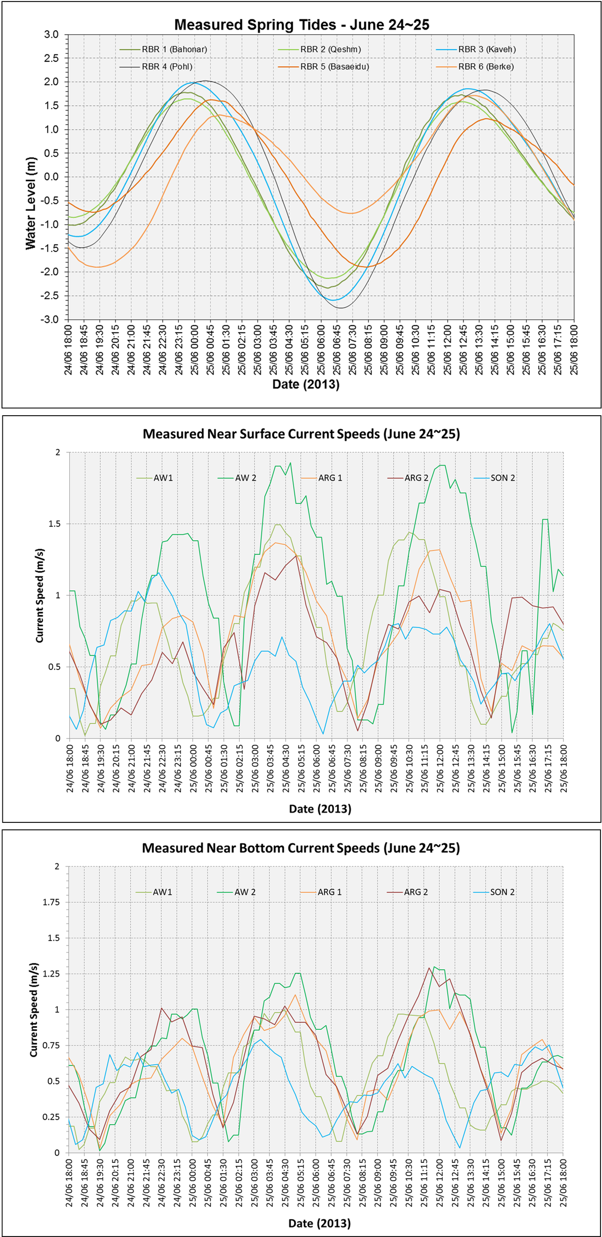
Measurements during the spring tide event of June 24th -26th 2013 in the study area, (top) water level variations; (middle) near surface current speed, and (bottom) near bottom current speed.
The analysis of the hydrodynamic environment and sediment transport processes in the study area highlights significant spatial and temporal variability. Water level measurements from tide gauges deployed over six months revealed considerable tidal fluctuations, with the highest recorded tidal range of 4.8 m at spring tide. The observed spatial differences in tidal dynamics suggest localized influences, as tidal ranges at Bahonar reached 4.1 m and Qeshm accounted for at 3.75 m followed similar phases, whereas Basaeidu measured at 3.5 m. Temporal variations in tidal behavior were also evident, with differing lag times in high and low tides across the monitoring locations (Figure 13). These differences underscore the complexity of tidal wave propagation and its modulation by local geomorphology and bathymetric features. ADCP measurements further confirmed the presence of strong tidal currents, with near-surface velocities reaching 1.85 m/s and near-bottom velocities around 1.25 m/s. The symmetry in ebb and flood currents suggests a well-balanced tidal regime, which plays a crucial role in sediment transport dynamics (Figure 13).
The field observations, together with relevant literature (Parhizkar et al., 2021; Zaker et al., 2010; Sadeghi et al., 2009), have been incorporated in this research to substantiate the claims regarding mangrove impacts on hydrodynamics and sediment transport, as well as the complexities of tidal wave propagation in the KS. Evidence for this can be seen in the observed differences in tidal characteristics recorded during the field campaign. Field measurements revealed significant variations in both tidal range and phase across the deployed tide gauge stations. For instance, on June 25, 2013, the tidal range varied from approximately 3.5 m at Basaeidu station to 4.8 m at the proposed bridge location (Pohl). Additionally, the tidal curves at Berke and Basaeidu show clear asymmetry and complex phase interactions, including cases where the higher high tide occurs at one station but not the other. These differences reflect the complex dynamics of tidal wave propagation, strongly affected by local geomorphological and bathymetric conditions. This is evident in the phase lag of up to 85 minutes observed at Basaeidu and in the skewed tidal patterns recorded at Berke. The distinctly different shapes of the tidal curves at Basaeidu and Berke, compared with those at Laft, Pohl, Bahonar, and Qeshm (Figure 13), point to the role of mangrove forests as a barrier to water flow from the strait toward the western side of the island and their influence on tidal modification. The significant spatial differences in tidal range and phase, including delays between tide gauge stations, highlight the complexity of tidal wave propagation shaped by the strait’s geomorphology and bathymetry.
When the Froude number, which represents the ratio of inertial to gravitational forces, exceeds a value of 1, the flow is considered supercritical. Under these conditions, the formation of upstream-migrating bedforms known as antidunes becomes possible on the seabed. However, as illustrated in Figure 12, the Froude number in this channel is well below unity, indicating that the flow is subcritical and the development of antidunes is not expected.
The impact of tidal currents on sediment transport is particularly evident in the dynamic sand dunes forming beneath the proposed bridge. The resulting erosion and deposition around the bridge piers underscore the growing need for the design team to evaluate sediment transport potential, its rate, and the surrounding morphological conditions. These dunes, ranging in height from 2 to 6 meters with wavelengths of 100–150 meters, indicate active sediment movement. However, hydrographic surveys conducted over a one-month period showed minimal dune migration, suggesting a stable sediment transport regime. The lack of significant movement implies that the sediment dynamics are primarily governed by the symmetrical nature of the tidal currents rather than episodic extreme events.
The present study indicates that wave action plays a negligible role in sediment transport within the KS, as it is largely obstructed by locating between Qeshm Island and the main land. Instead, strong tidal currents dominate the hydrodynamic processes, contributing to the dynamic sand dune formation in the narrowest sections of the strait. Despite the high-energy environment, fine sediments are present in certain areas, some of which are likely produced in the mangrove forests and the rest are coming through the streams discharging in to the area. The mangrove ecosystem contributes to sediment dynamics by trapping, breaking down, and redistributing organic and inorganic materials and play an important role in hindering the currents during tidal cycles. The mangrove ecosystems contribute to modifying the hydrodynamics and sediment production and distribution within the strait, with implications for coastal morphology and ecosystem stability. Hence, the strong tidal currents with the effective sediment transport in both sand transport and fine sediment transport are the controlling mechanism in this important body of water.
The collected data provide valuable insights into the hydrodynamic variability of the middle part of the KS, which understanding these processes is essential for bridge design, particularly in mitigating potential scour around bridge piers. Moreover, the findings serve as a foundation for numerical modeling efforts, enabling more accurate predictions of tidal and sediment transport behaviors. To conclude, the results underscore the need for continued monitoring and modeling to enhance coastal infrastructure resilience in dynamic tidal environments.
7 Summary and conclusion
This study applied validated regional and local hydrodynamic and sediment transport models to simulate tidal behavior and sediment dynamics in the KS, north of Qeshm Island in the PG. The models showed strong agreement with observed water levels and velocities, with correlation coefficients above 0.95 and low error values, confirming their reliability. Results indicate that tidal currents, reaching up to 1.85 m/s, are the primary driver of sediment transport, shaping dune mobility, localized erosion, and sedimentation patterns, while wave action plays a minor role. Annual siltation at Rajaee Port was estimated at about 132,000 m³, consistent with field measurements.
Field observations and modeling highlight the dynamic but stable nature of sediment transport in the KS. The central strait is dominated by mobile sand dunes and rocky beds, while sheltered eastern and western areas are influenced by fine sediments from the mainland and mangrove zones. Distinct asymmetries in tidal curves, phase lags of up to 95 minutes, and the modifying role of mangroves emphasize the complex interplay between hydrodynamics and geomorphology.
The findings provide important insights for sediment management, mangrove ecosystem protection, and infrastructure planning, especially for the proposed PG Bridge. The research contributes a valuable modeling framework, applicable to other semi-enclosed tidal environments, and underscores the importance of combining field data with numerical simulations.
Future work should include longer field campaigns, periodic hydrographic surveys, and incorporation of wave effects, spatially variable bed roughness, and expanded model domains. Moving toward three-dimensional modeling is also recommended to better capture vertical flow structures and improve predictions of sediment dynamics and morphological stability in the KS.
Statements
Data availability statement
The raw data supporting the conclusions of this article will be made available by the authors, without undue reservation.
Author contributions
MH: Methodology, Software, Validation, Writing – original draft, Writing – review & editing. MS: Conceptualization, Supervision, Validation, Writing – review & editing. ET: Conceptualization, Methodology, Data curation, Writing – review & editing, Resources, Supervision, Project administration. SH: Investigation, Methodology, Project administration, Resources, Supervision, Validation, Writing – review & editing.
Funding
The author(s) declared that financial support was not received for this work and/or its publication.
Acknowledgments
The authors would like to thank Mohammad Dibajnia, Ali Dastgheib, Ali Naeimi, Arash Bakhtiari, Aref Farhangmehr and Mehrnoosh Abbasian, for their collaborative efforts and expertise which enriched our research. We would like to extend our appreciation to Darya Negar Pars Consulting Engineers for helping us with data collection and S. Ebrahim Astaneh for providing the aerial photo of the Mangrove Forest – north of Qeshm Island.
Conflict of interest
The authors declare that the research was conducted in the absence of any commercial or financial relationships that could be construed as a potential conflict of interest.
Generative AI statement
Any alternative text (alt text) provided alongside figures in this article has been generated by Frontiers with the support of artificial intelligence and reasonable efforts have been made to ensure accuracy, including review by the authors wherever possible. If you identify any issues, please contact us.
Correction note
This article has been corrected with minor changes. These changes do not impact the scientific content of the article.
Publisher’s note
All claims expressed in this article are solely those of the authors and do not necessarily represent those of their affiliated organizations, or those of the publisher, the editors and the reviewers. Any product that may be evaluated in this article, or claim that may be made by its manufacturer, is not guaranteed or endorsed by the publisher.
References
1
Ancey C. Bohorquez P. Bardou E. (2014). Sediment transport in mountain rivers. Ercoftac100, 37–52. Available online at: https://www.researchgate.net/publication/267763188_Sediment_Transport_in_Mountain_Rivers (Accessed October 15, 2014).
2
Armstrong C. Howe J. A. Dale A. Allen C. (2021). Bathymetric observations of an extreme tidal flow: Approaches to the Gulf of Corryvreckan, western Scotland, UK,” Cont. Shelf. Res.217, 104347. doi: 10.1016/j.csr.2021.104347
3
Belderson N. Johnson R. H. Kenyon M. A. (1982). “ Offshore tidal sands: Processes and deposits,” in offshore tidal sands (Dordrecht: Springer) 58–94. doi: 10.1007/978-94-009-5726-8_4
4
Benjamins S. Dale A. Van Geel N. Wilson B. (2016). Riding the tide: Use of a moving tidal-stream habitat by harbour porpoises. Mar. Ecol. Prog. Ser.549, 275–288. doi: 10.3354/meps11677
5
Besio G. Blondeaux P. Brocchini M. Hulscher S. J. M. H. Idier D. Knaapen M. A. F. et al . (2008). The morphodynamics of tidal sand waves: A model overview. Coast. Eng.55, 657 670. doi: 10.1016/j.coastaleng.2007.11.004E
6
Bird E. C. F. (2008). Coastal géomorphlogy: An Introduction 2nd ed. (Hoboken, NJ, USA: Wiley), 411.
7
Campbell A. R. Simpson J. H. Allen G. L. (1998). The dynamical balance of flow in the Menai Strait. Estuar. Coast. Shelf. Sci.46, 449–455. doi: 10.1006/ecss.1997.0244
8
Davies A. G. Robins P. E. (2017). Residual flow, bedforms and sediment transport in a tidal channel modelled with variable bed roughness. Geomorphology295, 855–872. doi: 10.1016/j.geomorph.2017.08.029
9
Deltares (2021). Simulation of multi-dimensional hydrodynamic flows and transport phenomena, including sediments (Delft, Netherlands: Delft Hydraulic).
10
DNP (Darya Negar Pars Consulting Engineers) (2013). Field measurements in the Khuran Strait. (Tehran) 2–20.
11
Draper S. Adcock T. A. A. Borthwick A. G. L. Houlsby G. T. (2014). Estimate of the tidal stream power resource of the Pentland Firth. Renew. Energy63, 650–657. doi: 10.1016/j.renene.2013.10.015
12
Doré A. Bonneton P. Marieu V. Garlan T . (2016). Numerical modeling of subaqueous sand dune morphodynamics. J. Geophys. Res. Earth Surf. 121, 565–587. doi: 10.1002/2015JF003689
13
Eliassen I. K. Heggelund Y. Haakstad M. (2001). A numerical study of the circulation in Saltfjorden, Saltstraumen and Skjerstadfjorden. Cont. Shelf. Res.21, 1669–1689. doi: 10.1016/S0278-4343(01)00019-X
14
Engelund F. Hansen E. (1967). A Monograph on sediment Transport in Alluvial Streams (Copenhagen, Denmark: Teknisk Forlag).
15
Ernstsen V. B. Noormets R. Winter C. Hebbeln D. Bartholomä A. Flemming B. W. et al . (2006). Quantification of dune dynamics during a tidal cycle in an inlet channel of the Danish Wadden Sea. Geo-Mar. Lett. 26, 151–163. doi: 10.1007/s00367-006-0026-2
16
Guerra J. V. Ogston A. S. Sternberg R. W . (2006). Winter variability of physical processes and sediment-transport events on the Eel River shelf, northern California. Continental Shelf Research26 (17–18), 2050–2072. doi: 10.1016/j.csr.2006.07.002
17
Haghshenas S. A. Bakhtiari A. Jedari Attari M. Razavi Arab A. Emami A. D. (2014). “ Strong currents and dynamic sand waves in the khuran strait, qeshm island”, the persian gulf,” in the Persian Gulf, 17th Physics of Estuaries and Coastal Seas (PECS) Conference (Pernambuco, Brazil: Porto de Galinhas) 19–24. October 2014.
18
Hoseini Chavooshi S. M. Kamalian R. (2024). A Process-based calibration Procedure for Non-Cohesive Silt Transport Models at Shahid Rajaee Port Access Channel. ijmt19, 43–56. Available online at: http://ijmt.ir/article-1-825-en.html (Accessed February 28, 2024).
19
Huang X. Peng F. (2013). Sediment transport dynamics in ports, estuaries and other coastal environments. Sediment. Transp. Process. Their. Model. Appl., 2–36. doi: 10.5772/51022
20
Imasato N. Awaji T. Kunishi H. (1980). Tidal exchange through Naruto, Akashi and Kitan Straits. J. Oceanogr. Soc.36, 151–162. doi: 10.1007/BF02072060
21
Jedari Attari M. (2025). An integrated three-dimensional water and multilayer sediment quality model for Tokyo Bay. Acta Geophys.73, 2683–2724. doi: 10.1007/s11600-025-01548-y
22
Karpenko M. Stosiak M. Šukevičius Š . (2023). Hydrodynamic processes in angular fitting connections of a transport machine’s hydraulic drive. Machines11 (3), 355. doi: 10.3390/machines11030355
23
Jedari Attari M. Farhangmehr A. Bakhtiari A. Delkhosh E. Ameri F. Hamidian Jahromi E. et al . (2024). A 45-year updating wind and wave hindcast over the Oman Sea and the Arabian Sea. Reg. Stud. Mar. Sci.80, 103882. doi: 10.1016/j.rsma.2024.103882. ISSN 2352-4855.
24
Kondolf G. M. Montgomery D. R. Piégay H. Schmitt L. (2005). Geomorphic classification of rivers and streams. doi: 10.1002/0470868333.ch7
25
Le Hir P. Roberts W. Cazaillet O. Christie M. Bassoullet P. Bacher C. (2000). Characterization of intertidal flat hydrodynamics. Cont. Shelf. Res.20, 1433–1459. doi: 10.1016/S0278-4343(00)00031-5
26
Li C. Weeks E. (2009). Measurements of a small-scale eddy at a tidal inlet using an unmanned automated boat. J. Mar. Syst.75, 150–162. doi: 10.1016/j.jmarsys.2008.08.007
27
Lin Y. Fissel D. B. (2014). High resolution 3-d finite-volume coastal ocean modeling in lower Campbell River and discovery passage, British Columbia, Canada. J. Mar. Sci.2, 209–225. doi: 10.3390/jmse2010209
28
Lin Y. Jiang J. Fissel D. B. Foreman M. G. Willis P. G. (2016). Application of finite-volume Coastal Ocean Model in studying strong tidal currents in Discovery Passage, British Columbia. Canada. J. Coast. Res.32, 582–595. doi: 10.2112/JCOASTRES-D-15-00046.1
29
Lora Jane Dillon D. W. (1995). An initial evaluation of potential tidal stream development sites in Pentland Firth, Scotland. in Proc. World Renewable Energy Congress X, Glasgow, Scotland (Berlin: Elsevier) 6, 181–189.
30
MEWE (Middle East Water and Environment) (2021). Updating sediment studies for 12 ports; final measurements report.
31
Parhizkar F. Rajabi M. Yamani M. Mokhtari D. (2021). Analysis of changes in the range of mangrove forests in the north and east of the Strait of Hormuz affected by coastal morphology and hydrodynamics of the Persian Gulf. J. Hydrogeomorphol.7, 61–84. Available online at: https://hyd.tabrizu.ac.ir/article_12657_064e519cb1aa41160311268e23cfd342.pdf (Accessed March 2, 2021).
32
Partheniades E. (1965). Erosion and deposition of cohesive soils. J. Hydraul. Division.91, 105–139. doi: 10.1061/JYCEAJ.0001165
33
Richardson J. F. Zaki W. N. (1954). The sedimentation of a suspension of uniform spheres under conditions of viscous flow. Chem. Eng. Sci.3, 65–73. doi: 10.1016/0009-2509(54)85015-9
34
Sadeghi A. Tajziehchi M. Chegini V. Ghasemizadeh H. (2009). “ Hydrodynamic modeling of the Khuran Strait under the influence of tidal currents,” in Proceedings of the 11th National Conference on Marine Industries of Iran (Kish Island, Iran: Persian).
35
van Maren D. S. van Kessel T. Cronin K. Sittoni L. (2015). The impact of channel deepening and dredging on estuarine sediment concentration. Continent. Shelf. Res.95, 1–14. doi: 10.1016/j.csr.2014.12.010
36
Van Rijn L. C. (1993). Principles of sediment transport in rivers, estuaries and coastal seas ( Aqua Publications) 654.
37
Van Rijn L. C. Roelvink J. A. Horst W. T . (2000). Approximation formulae for sand transport by currents and waves and implementation in DELFT-MOR, Tech. Rep. Z3054.40 WL. (Delf, The Netherlands: Delft Hydraulics).
38
Van. Rijn L. C. (2001). General view on sand transport by currents and waves: data analysis and engineering modelling for uniform and graded sand (TRANSPOR 2000 and CROSMOR 2000 models). Z2899.20 / Z2099.30 / Z2824.30. WL (Delft, The Netherlands: Delft Hydraulics).
39
Van Rijn L. C. (2003). “ Sediment transport by currents and waves; general approximation formulae Coastal Sediments,” in Corpus Christi (USA: In Corpus Christi).
40
Whipple K. (2019). Essentials of sediment transport motivational example: synthetic sediment transport data. ISH. J. Hydraulic. Eng.0971–5010, 11. Available online at: https://ocw.mit.edu/courses/earth-atmospheric-and-planetary-sciences/12-163-surface-processes-and-landscape-evolution-fall-2004/lecture-notes/4_sediment_transport_edited.pdf.
41
Xie D. Gao S. Wang Z. B. Pan C. Wu X. Wang Q. (2017). Morphodynamic modeling of a large inside sandbar and its dextral morphology in a convergent estuary: Qiantang Estuary, China. J. Geophys. Res. Earth Surf.122, 1553–1572. doi: 10.1002/2017JF004293
42
Xie D. Pan C. Gao S. Wang Z. B. (2018). Morphodynamics of the Qiantang Estuary, China: Controls of river flood events and tidal bores. Mar. Geol.406, 27–33. doi: 10.1016/j.margeo.2018.09.003
43
Xie D. Wang Z. B. (2021). Seasonal tidal dynamics in the Qiantang Estuary: The importance of morphological Evolution. Front. Earth Sci.9. doi: 10.3389/feart.2021.782640
44
Xing Q. G. Loisel H. Schmitt F. G. Dessailly D. Hao Y. J. Han Q. Y. et al . (2012). Fluctuations of satellite-derived chlorophyll concentrations and optical indices at the Southern Yellow Sea. Aquat. Ecosyst. Health Manage.15 (2), 168–175. doi: 10.1080/14634988.2012.68848
45
Zaker N. H. Ghaffari P. Jamshidi S. Nourian M. (2010). “ Dynamics of the currents in the Strait of Khuran in the Persian Gulf,” in Second International Conference on Coastal Zone Engineering and Management (Arabian Coast 2010), Muscat, Oman, November 1–3, (Delft: International Association for Hydro-Environment Engineering and Research (IAHR). Available online at: https://www.iahr.org/library/infor?pid=20020.
Summary
Keywords
the Khuran strait, the persian gulf, numerical modeling, sediment transport, tidal currents, sand dunes
Citation
Hajibaba M, Soltanpour M, Taheri E and Haghshenas SA (2026) Tidal currents and the dynamics of sand dunes in the Khuran strait – the Persian gulf. Front. Mar. Sci. 12:1481841. doi: 10.3389/fmars.2025.1481841
Received
16 August 2024
Accepted
31 October 2025
Published
07 January 2026
Corrected
03 February 2026
Volume
12 - 2025
Edited by
Guan-hong Lee, Inha University, Republic of Korea
Reviewed by
Wenjian Li, Chinese Academy of Sciences (CAS), China
Mykola Karpenko, Vilnius Gediminas Technical University, Lithuania
Updates
Copyright
© 2026 Hajibaba, Soltanpour, Taheri and Haghshenas.
This is an open-access article distributed under the terms of the Creative Commons Attribution License (CC BY). The use, distribution or reproduction in other forums is permitted, provided the original author(s) and the copyright owner(s) are credited and that the original publication in this journal is cited, in accordance with accepted academic practice. No use, distribution or reproduction is permitted which does not comply with these terms.
*Correspondence: Maryam Hajibaba, maryam_hajibaba@email.kntu.ac.ir; S. Abbas Haghshenas, sahaghshenas@ut.ac.ir
ORCID: Maryam Hajibaba, orcid.org/0000-0003-0592-1370; S. Abbas Haghshenas, orcid.org/0000-0003-4297-093X
Disclaimer
All claims expressed in this article are solely those of the authors and do not necessarily represent those of their affiliated organizations, or those of the publisher, the editors and the reviewers. Any product that may be evaluated in this article or claim that may be made by its manufacturer is not guaranteed or endorsed by the publisher.