Abstract
Understanding the characteristics of breaking waves in deep and intermediate waters is crucial for air-sea interactions. Recent advancements in modelling these interactions have often relied on numerical wave tanks using Stokes waves, which may not fully represent real-world conditions. To address this gap, we developed a numerical wave tank to investigate the effects of different turbulence models on the performance of our numerical wave model in simulating breaking waves under more realistic wave conditions. A hybrid model that couples a Lagrangian wave model with a VOF model based on OpenFOAM is developed to simulate breaking wave groups resulting from dispersive focussing, with a spectrum related to a modelled sea state. The numerical results obtained through the hybrid wave model without turbulence models are validated against experimental data, demonstrating a high level of accuracy. Then, four turbulence models including RANS standard k − ϵ, RNG k − ϵ models, LES Smagorinsky and LES k-equation turbulence models are applied to the hybrid wave model with peak-focussed wide band Gaussian (GW) spectrum. The effects of turbulence models on the prediction of breaking crests, the energy dissipation due to breakers and the estimation of the breaking strength parameter b are investigated. The findings demonstrate that the turbulence models can significantly affect the numerical results for weak breaking cases. Notably, the hybrid wave model with the LES k-equation turbulence model showed superior performance. This proposed numerical wave tank can be a promising tool for investigating air-sea interactions in 3D simulations under more realistic wave conditions.
1 Introduction
In recent decades, the study of breaking waves in deep and intermediate waters has gained significant attention due to its profound implications for air-sea interaction. However, accurately capturing the physical characteristics of breaking waves through field observations and laboratory experiments presents significant challenges. Breaking waves involve rapid changes in velocity and surface elevation, requiring high-speed and high-resolution measurement techniques. Capturing the full velocity field and precise wave crest shapes is challenging; for example, velocity at the crest surface often relies on extrapolation from other points due to measurement difficulties. Additionally, calculating energy dissipation in a wave tank typically uses volume control analysis, which demands indirect estimations and leads to uncertainties because it is impractical to measure all details along the flume. Numerous efforts have been dedicated to simulating the intricate physical processes involved in breaking waves in deep and intermediate waters using Stokes wave models, e.g. Chen et al. (1999); Song and Sirviente (2004); Iafrati (2009); Lubin and Glockner (2015); Deike et al. (2016); Wang et al. (2016); Yang et al. (2018); Di Giorgio et al. (2022); King et al. (2023). However, the physical processes involved in wave breaking should also be investigated under controlled and more realistic wave conditions. For example, wave groups with wide and narrow band Gaussian, JONSWAP and Pierson-Moskowitz spectrum can be used as input wave conditions for studying the breaking behaviour (Buldakov et al., 2017).
It is widely acknowledged that wave breaking generates a broad spectrum of turbulent scales, ranging from large-scale eddies to micro-scale eddies. Attempting to model breakers through Direct Numerical Simulation (DNS) with the aim of resolving motions across this entire range of scales can quickly surpass the computational capacity of available computers. Consequently, smaller-scale eddies remain unresolved in such simulations. From a physical perspective, there exists interactions among motions at all scales during the post-breaking phases. Neglecting the influence of smaller scales on the larger ones can lead to inaccuracies in the results for the larger scales. In such circumstances, turbulence models can provide more accurate overall effects of unresolved small turbulent scales on larger ones for breakers. However, turbulence models for simulating breaking waves in deep and intermediate waters have garnered less attention when compared to their counterparts in coastal engineering. In the early studies, k − ϵ turbulence model with the VOF method had been applied to model the wave breaking on the bench for Reynolds-averaged Navier-Stokes equations (RANS) simulations (Lemos, 1992; Lin and Liu, 1998). Reasonable agreement between numerical and experimental results had been achieved by choosing appropriate model coefficients of turbulence models. More recently, several studies have focussed on improving RANS simulations for modelling breaking waves using OpenFOAM. Brown et al. (2016) assessed various RANS turbulence models for onshore wave breaking. Comparisons between the wave surface profiles, velocity and Turbulence Kinetic Energy (TKE) with and without turbulence models showed varying effects of turbulence models between spilling and plunging breakers. In order to solve the over-prediction of turbulent intensity during the wave propagation caused by the turbulence closure model, attempts have been made by modifying the k − ω and k − ω SST RANS turbulence models (Devolder et al., 2018; Larsen and Fuhrman, 2018), showing improved results with insignificant diffusion and reduced over-production of pre-breaking turbulence in the surf zone. Later, Fuhrman and Li (2020) studied the instability of the realizable k − ϵ model using the similar method developed by Larsen and Fuhrman (2018) to formally stabilise the standard k − ϵ RANS model for the wave train and breaking over a bench, showing encouraging results. Li et al. (2022) then newly applied the Reynolds stress-ω turbulence closure model to the wave breaking in the surf zone, demonstrating that this model naturally avoid unphysical exponential growth of turbulence prior to breaking. Although RANS turbulence models are infrequently utilised in simulations of deep-water wave breaking, Li and Fuhrman (2022) applied the Reynolds stress-ω turbulence closure model to investigate the two-dimensional Benjamin–Feir instability, demonstrating its effectiveness in predicting surface elevation.
Compared to RANS turbulence models mentioned above (e.g. the k − ϵ model) where the flow equations are averaged in time and only the mean velocity field is obtained from the model according to the size of the grid, Large Eddy Simulation (LES) has attract considerable attention for modelling the turbulent flow at high Reynolds number. In LES, the large-scale turbulence fluctuations are directly resolved by the governing equations and the sub-grid scale turbulence model is used to represent the effect of the small-scale turbulence which is not resolved by the governing equations. LES simulation applies spatial filtering for the governing equations and the width of the filter is dependent of the grid size. A larger part of turbulence motion will be resolved directly if a finer grid is imposed. Christensen and Deigaard (2001) and Christensen (2006) conducted LES simulation for wave breaking over a constant slope by coupling different interface capturing and tracking methods, the Marker and Cell (MAC) and the Volume of Fluid (VOF), respectively, with standard Smagorinsky and k-equation sub-grid turbulence models. Compared to the laboratory data, both LES turbulence sub-grid models over-predicted wave heights before breaking and delayed the predicted onset of breaking. In studies of LES simulation for steepness-limited breaking waves (breaking waves in deep and intermediate waters), Lubin et al. (2006) simulated plunging breakers induced by a first-order Stokes wave with large initial steepness propagating through a flat bottom in a three-dimensional numerical wave tank, employing a dynamic subgrid-scale turbulence model. Their studies were intent to present the capability of their model to generate the overall features of breakers and then provide a quantitative analysis of the large scale of air entrainment due to plunging. However, the effects of turbulence model were not carefully investigated. Utilising a 3D LES/VOF turbulence model coupled with a bubble entrainment model, Derakhti and Kirby (2014) investigated the interaction between liquid and bubbles during deep-water wave breaking caused by dispersive focussing. They analysed the performance of the two-phase TKE transport equation compared to the single-phase TKE transport equation on the subgrid-scale dissipation rate. Furthermore, Lubin and Glockner (2015) used a 3D LES/VOF turbulence model with fine mesh resolution to study the evolution of vortex filaments for a single unstable periodic sinusoidal wave of large amplitude. In their investigations, details of physical phenomena were presented and discussed, but the effects of the LES turbulence model were not mentioned. Later, Derakhti et al. (2020) utilised the LES/VOF numerical wave tank developed by Derakhti and Kirby (2014) to study the breaking criteria for wave breaking in deep and intermediate waters. More recently, LES simulations have been used to study the problems of bubble generation induced by wave breaking (King et al., 2023; Liu et al., 2024). Although turbulence due to breakers is a 3D phenomenon, when computational resources are limited, applying LES in 2D simulations can result in improved performance compared to simulations without turbulence models for certain specific aspects. For example, Zou and Chen (2017) used a Navier-Stokes (NS) solver in OpenFOAM with a LES model and a VOF technique to study wind and current effects on wave formation and breaking in deep water. Additionally, Cui et al. (2022) studied the wave geometry, kinematic and dynamic characteristics of focussed breaking waves in finite water depth with different wave steepness using 2D LES simulations.
An ever-increasing body of literature shows that the advantages of hybrid models in the simulation of breaking waves become recognised over the last two decades. The basic concept of hybrid models regarding the simulation of the ocean breaking waves is to couple two different numerical models for simulating the same event but playing different roles in different phases of the evolution. In such a method, the Fully Nonlinear Potential Flow Theory (FNPT) usually may be the first candidate to run a fast simulation of wave generation and propagation and then full CFD models may be used to simulate the phases when the breakers take place. Hybrid models combine the advantages of FNPT models for long-term and long-distance simulation with higher accuracy and higher computational efficiency for the phases prior to the onset of breaking with the ability of CFD models to continue calculating after the wave crest touches the free surface (Lachaume et al., 2003; Biausser et al., 2004). In the meanwhile, the CFD models are capable of resolving the violent breaking process with strong turbulence for the subsequent phases after breaking onset, but it is computationally expensive. Hence, the combination of these two types of models can potentially meet the needs of different purposes at different stages of modelling for a whole wave-breaking event, thus increasing the accuracy and reducing the computational costs. In general, the coupling techniques can be categorised into weak couplings and strong couplings of two models.
For the weak coupling method, the information between two models is transferred from one to the other in one direction, in which the first model will be run independently until a phase which is undesired and then the information from the first model will be fed into the second model as initial conditions for running the following phases. For the strong coupling method, the information from two models are exchanged via a coupling zone and the solutions from both models will be mutually affected and dependent (Sriram et al., 2014). In the studies using the weak coupling techniques, Hildebrandt et al. (2013) employed the weak coupling/one-way coupling approach to shorten the computational effort through running the fast FNPT model for the first stage of the whole simulation and then running the NS model for the detailed investigation of the small scale phenomenon, e.g. viscous effects, turbulence. According to the comparison of wave profiles between FNPT-3D VOF and 2D-3D VOF models, the wave profiles from the FNPT-3D VOF model gave better performance compared to that from the sole usage of VOF models, which might benefit from the highly accurate simulation of wave propagation for a long time and long distance using fast and stable FNPT models. More recently, Buldakov et al. (2019) proposed a new modified Lagrangian numerical wave model, in which a dispersion correction and a treatment of crest shape correction have been implemented in order to reduce the dispersion errors and continue the calculation through the whole breaking processes. This new version of the Lagrangian model was found to reproduce a remarkably good quality of breaking due to the dispersive focussing by comparing the modelled results against the experimental measurements for the weakly spilling breaking. This Lagrangian wave model was suggested as an alternative to classical FNPT models as a fast component in a hybrid model. In particular, Lagrangian models offer an advantage over FNPT models by capturing vortical flows, enabling wave simulations over sheared currents. In the inviscid Lagrangian formulation, vorticity remains constant and is defined by Lagrangian labels, allowing a simple application to arbitrary shear flows. This feature is also useful for modelling wave behaviour after breaking, where intense vortical motion occurs beneath the surface. Followed by Chen et al. (2019), they coupled this Lagrangian model with a NS OpenFOAM model for modelling the focussing wave groups and sheared current interacting with a vertical cylinder. One-way coupling method was applied by adapting the free-surface elevation and flow kinematic time histories on the numerical boundaries from the Lagrangian model into a truncated 3-D numerical OpenFOAM wave domain as initial conditions of the OpenFOAM model. The modelled surface elevation and harmonic components of the wave loading on the larger cylinder were analysed carefully by the comparisons between the numerical and experimental datasets. The generation and iteration of wave-on-current focussing waves simulated by the faster Lagragian model provided the accurate modelled data which helped improving the overall accuracy and shortening the computational time compared to that of direct simulation of the whole event by only using the OpenFOAM model. Lately, Higuera et al. (2021) updated two approaches of one-way coupling method in which the Lagrangian model was coupled with the olaFlow CFD model by passing the information from one to the other through the boundary or a relaxation zone for simulating the steep waves interacting with a cylinder. In their study, the Lagrangian model was also used to generate the incoming waves and then provided the free surface elevation and kinematics as the input for the olaFlow CFD model in the second part of the simulation. The coupling method via the fixed-value boundary is similar to that of Chen et al. (2019), but the coupling method via the relaxation zone requires inputting data over the whole area of the relaxation zone at each time step by several interpolations in time and space. The advantage of this method via relaxation zone is that it does not require premature wave conditions, which means the data selected from the dataset of the Lagrangian model can be at any time point. On that account, it is considered to be more flexible compared to that of the coupling method via the boundary.
For the two-way coupling techniques, Narayanaswamy et al. (2010) used the strong coupling approach to combine a Boussinesq model (FUNWAVE) with a Smoothed Particle Hydrodynamics (SPH) model (SPHysics) for developing a hybrid model of wave simulation with a virtual feedback boundary between two subdivided regions for the solitary waves advancing along the constant water depth. Kim et al. (2010) applied a transmission domain for the exchange of information between a Boundary Element Method (BEM) model and a VOF model for the propagation of random waves. Although these studies have shown the good accuracy of modelling the waves via the two-way coupling hybrid approach, they were intent to test the applicability of hybrid models in modelling wave propagation without the occurrence of turbulence. Sriram et al. (2014) made an outstanding study of the strong coupling method which coupled FNPT and NS models for modelling regular waves and the wave overtopping on a slope. A novel method to adapt the exchange of information between two models over a lapping zone has been developed, which allows one side of the boundary of the transmission zone to deform as a curve during the process of exchanging information between two models. The comparisons between surface profiles and pressure distribution between numerical models and the experimental measurements have shown that the hybrid model can be a promising method to simulate ocean wave events with a high level of accuracy and less computational effort. Generally, either one-way or two-way coupling methods, the important parts of successful modelling of wave events using a hybrid method may be depending on adequate algorithms which can adapt the information between two different models and interpolate the necessary data in correct coordinates of the numerical domain.
The review presented highlights two critical gaps in the existing research that warrant attention. Firstly, the existing systematic studies of the effects of turbulence models in breaking wave modelling mainly focussed on breakers in a coastal area, which cannot provide sufficient information to understand how they affect the evolution of breaking in deep and intermediate waters. Secondly. there have been notable advancements in the development of hybrid wave models for simulating breaking waves, further efforts are required to improve the accuracy of transferring wave conditions between these models. Such advancements could potentially enhance their utility as reliable numerical wave tanks for investigating post-breaking processes.
The objectives of the present work have two important aspects:
To develop and validate a hybrid wave model which couples a Lagrangian wave model with a VOF model based on OpenFOAM for accurately reproducing breaking wave groups induced by dispersive focussing against experimental measurements, with a spectrum related to a realistic modelled sea state.
To investigate the effects of different turbulence models within the framework of the developed hybrid wave model, including RANS standard k−ϵ, RNG k−ϵ models, LES Smagorinsky and LES k-equation turbulence models.
The paper is organised as follows. The physical setups are briefly described in Section 2. The mathematical formulations for the numerical models are presented, followed by the numerical setups of the hybrid wave model in Section 3. The results of the mesh resolution study and the validation of our numerical simulations are demonstrated in Section 4. The results of the effects of turbulence models are discussed in Section 5. Finally, the conclusions based on the present analysis are drawn in Section 6.
2 Experimental results
The time histories of the experimental data used for validation in this study were recorded through a series of probes in the wave flume at the Civil Engineering department of UCL (University College London). The digitalised entire wave profiles were extracted through the post-processing of highs-peed camera images from Buldakov et al. (2017). The physical flume itself has a width of 0.45 m, and the working section which is located between two piston wavemakers spans a length of 13 m. A Cartesian coordinate system denoted as Oxz, is adopted in both the physical and numerical wave flumes. In this coordinate system, the origin x = 0 corresponds to the plane of the undisturbed free surface at midpoint of the flume and the positive z-direction extends upward. One wave maker situated at one end of the flume generates wave components in accordance with the provided input signal, while the other wave maker situated at the opposite end serves for active reflection absorption. The operation of the wavemaker is governed by a force feedback system that operates within the frequency domain. The control system adopts discrete spectra and is responsible for generating periodic paddle motions. An overall return period utilised in this experiment was 64 s, signifying the time interval between successive recurring events generated by the paddle. The range of frequencies employed in the experiments ranged from 1/128 Hz to 4 Hz, encompassing 512 equally spaced discrete frequency components with a step size of 1/128 Hz. For all experimental tests, the water depth d is 0.4 m over the horizontal bed. Input wave components were focussed at the midpoint along the flume. For the cases presented in this study, the input wide-band Gaussian spectrum can be found in Figure 3 of Buldakov et al. (2017). The parameters of focussed wave groups with the wide-band Gaussian spectrum are as follows: the peak frequency is fp= 1 Hz with the linear phase velocity C1 = 1.46 m/s at this frequency and the group velocity U1 = 0.89 m/s. With a wavelength of λ1 = 1.46 m, the dimensionless water depth is d/λ1 = 0.274, thereby establishing intermediate depth conditions. Waves with linear peak focussed amplitudes of A = 6.4 cm, 6.8 cm, and 7.2 cm are generated by scaling the input of small waves with a peak amplitude of A = 2 cm by factors of 3.2, 3.4, and 3.6, respectively. These wave groups are characterised by a global steepness parameter SL, defined as , where an and kn are amplitudes and wave numbers of spectral components of the wave group. For the wave groups with A = 6.4 cm, 6.8 cm, and 7.2 cm, SL values are calculated as 0.3, 0.32, and 0.34, respectively. These waves are classified into strongly nonlinear non-breaking waves, extreme weak breaking waves, and strong breaking waves, respectively. More details of wave generation methodology and experimental settings can be found in Section 3 and 4, Buldakov et al. (2017). The Lagrangian wave model replicates the physical experiments. It is worth mentioning that during the focussing of a steep Gaussian wave group, a smooth long-frequency tail is developing, resulting in a non-linear spectrum that closely resembles the JONSWAP or Pierson–Moskowitz (PM) spectrum, though not identically. The breaking process is primarily influenced by the local behaviour of the focussed wave near the crest, which is more sensitive to spectral discontinuities than to the overall smoothness of the spectrum. Therefore, the spectrum used in this study provides a more realistic representation of breaking crest behaviour compared to spectra with sharp frequency cut-offs.
For the validation using the extraction of crest profiles at different instants, we acknowledge the valuable work of Chasapis Tassinis (2023), whose methods enabled the extraction of crest profiles from high-speed camera images. The crest shapes were obtained through post-processing of two-dimensional experimental image frames captured with high-speed cameras and a laser sheet, which illuminated the wave surface for enhanced edge detection. The methods for wave edge identification are detailed in Chasapis Tassinis (2023), and the data used in this study were provided by Chasapis Tassinis (2023).
3 Numerical setup
The hybrid wave model presented in this paper is implemented on OpenFOAM-v1906. In this hybrid model, the first component of the hybrid wave model is a Lagrangian wave model. This Lagrangian model is employed to generate waves with accurately predicted surface elevations and kinematics, which have been previously validated against experimental data prior to breaking onset. The wave generation is well controlled to ensure that waves are focussed at the designated focal point with the desired spectrum. A brief formulation of the Lagrangian model is provided in Appendix A. The detailed description of the wave generation and validation procedures for the Lagrangian wave model can be found in Buldakov et al. (2019).
In this section, we begin by presenting the formulation of our OpenFOAM-based numerical model, followed by a description of turbulence modelling. Subsequently, the implementation of the Lagrangian-OpenFOAM coupled model is introduced, along with an overview of the numerical settings applied to define the simulation domain.
3.1 Mathematical formulation
In our present work, we employ the InterIsoFoam solver, an extended version of the standard InterFoam solver. This solver tackles the Navier-Stokes equations for two incompressible, immiscible fluids. The flow simulation involves solving the conservation of mass and momentum equations, which are formulated as follows (Larsen et al., 2018).
where ui represents the mean components of the velocities, gi denotes gravitational acceleration, p represents pressure, ρ is the fluid density, µ = ρν is the dynamic molecular viscosity (ν being the kinematic viscosity) and Sij is the mean strain rate tensor given by . represents the surface tension term. σ is the surface tension constant. κ is the local mean curvature of the interface, which is approximated as with α being the continuous function. The continuous function α represents the volume fraction in each cell, satisfying the following equation:
where α must be conserved and bounded between 0 to 1 to keep the interface sharp. Cells with α =1 contain only liquid, cells with α = 0 are full of air, and cells with 0< α< 1 are wet cells, indicating they are partially occupied by water. The density and viscosity can be defined as
where ρwater, ρair and µwater, µair are the density and viscosity of the two fluids, water and air, respectively.
3.2 Turbulence modelling
The use of turbulence model is to represent the dissipative effect of the small turbulent structures with a turbulent viscosity. Four types of turbulence models are applied in the present work: Reynolds-averaged Navier-Stokes (RANS) k−ϵ model (standard k−ϵ model) and Re-normalisation Group k−ϵ model (RNG k−ϵ model), Large Eddy Simulation (LES) Smagorinsky model and Large Eddy Simulation (LES) k-equation model. In the following parts, brief descriptions of them in OpenFOAM framework are introduced, including explanations of the relevant initial values adopted for the turbulence models.
3.2.1 The k − ϵ model
To account for turbulence in various flow regimes, the Reynolds-averaged Navier-Stokes (RANS) Equations are derived from the instantaneous Navier-Stokes equations by Reynolds decomposition approach. The incompressible RANS equations have the forms for the time-averaged continuity equation and momentum equation (Giancarlo, 2009).
where is the time-averaged velocity and is the time-averaged pressure; is the Reynolds stress term, . To close this system of equations, τij needs to be expressed by the mean variables. The Boussinesq hypothesis assumes that the deviatoric part of the Reynolds stress is proportional to the rate of strain tensor of the mean flow, which writes
where µt is the turbulent viscosity, δij is the Kronecker delta, which equals 1 when i = j and 0 otherwise, K is the average kinetic energy of the velocity fluctuations;
and is the strain-rate tensor of the mean field
As shown in Equation 1, the turbulent viscosity µt is required to be calculated to close the equations. The k−ϵ model provides the one of the approaches to compute the turbulent viscosity µt by solving two additional transport equations.
In the version of OpenFOAM-v1906, it formulated the standard k−ϵ model developed by Launder and Spalding (1974), solving the following transport equations for the turbulent kinetic energy equation, k
The second equation describes the turbulent kinetic energy dissipation rate, ϵ
where , , are model coefficients. Then, the turbulent viscosity µt can be calculated as
where Cµ is the model coefficient for the turbulent viscosity. The suggested values of model coefficients are listed in Launder and Spalding (1974) based on extensive examinations of free turbulent flows. We tested our cases with various values of model coefficients and the values of these model coefficients suggested by Launder and Spalding (1974) provide good results for our cases. We found that the larger Cµ leads to overestimation of energy dissipation due to wave breaking. Therefore, we adopt the values of model coefficients suggested by Launder and Spalding (1974) as follows: .
In OpenFOAM, the initial value of the turbulent kinetic energy can be estimated by
in which I is turbulence intensity and uref is a reference flow speed. We take the crest velocity at focal point without turbulence model as the initial value of uref. The initial values I are set at 1% and 10% for weak and strong breaking cases, respectively. These values are based on reasonable estimations from the energy dissipation observed in cases without turbulence models.
The initial value of the turbulence dissipation rate can be estimated by
in which L is a reference length scale, which is a measure of the size of the eddies that are not resolved. In our case, we assume it to be the minimum length of the grid size.
3.2.2 The RNG k − ϵ model
The RNG k − ϵ model was developed by Yakhot et al. (1992) using a statistical technique to renormalise the instantaneous Navier-Stokes equations. Compared to the standard k − ϵ model which determines the eddy viscosity from a single turbulence length scale, the RNG k − ϵ model takes account of the effects of the different scales of motion by modifications to the production term for ϵ. The formulations of RNG k−ϵ model are similar to the standard k−ϵ model, in which the transport equation for k remains the same and an additional term is added to the transport equation for ϵ
where η = Sk/ϵ and S is the modulus of the mean rate of strain tensor, defined as .
The values of constant model coefficients are derived analytically in the RNG procedure. The model constants are: , , , , , , .
3.2.3 The Smagorinsky subgrid-scale (SGS) model
In the Large Eddy Simulation (LES), by filtering the Navier-Stokes equations, an additional stress term τsgs (subgrid stress term) is applied for modelling the effects of the eddies which cannot be resolved by the smallest mesh size in the simulation.
The filtered Navier-Stokes equations for incompressible flow can be expressed as
where indicates the filtering operator.
In order to close a large eddy formulation, the subgrid stress term τsgs is calculated by determining the subgrid kinematic viscosity νsgs. Different LES models use various methods to calculate νsgs. A key point to achieve a successful LES simulation is to choose the appropriate value of the sub-grid kinematic viscosity νsgs that can control the amount of energy dissipation correctly.
Smagorinsky (1963) proposed the first sub-filter-stress model using an eddy viscosity approach, which serves as a base for all other sub-grid-scale models. Sub-grid kinematic viscosity has the unit of [m2/s]. Based on the assumption of isotropic eddies, the relationship between νsgs, an eddy size and the velocity change across the eddy
where l0 is length scale of eddies and S0 is the corresponding velocity scale.
The scales can be expressed as
where Cs is called the Smagorinsky constant which is between 0 and 1; △ is the mesh size; Sij is strain rate tensor.
This finally gives following expression for
In OpenFOAM source code, the Smagorinsky constant Cs is represented by the model coefficients Ckand Ce
where Ck= 0.094 and Ce= 1.048.
3.2.4 The k-equation SGS model
Instead of involving the sub-grid velocity scale used in the Smagorinsky SGS model, Yoshizawa (1982) derived an one-equation SGS model which solves the sub-grid turbulence kinetic energy ksgs. The ksgs is determined by the following model transport equation
with the sub-grid kinematic viscosity . The default valued of the model coefficients in OpenFOAM are Ck= 0.094 and Cϵ= 1.048. We have tested model coefficients and found the default values can provide satisfactory results. To maintain consistency, we adopt the default values of model coefficients for all turbulence models.
3.3 Implementation of the Lagrangian-OpenFOAM coupled model
As we mentioned previously, for a one-way/weak coupling method, the main task to form a hybrid model is to transfer the data accurately from one model to the other. In this study, we have kinematic and dynamic data and the coordinates of Lagrangian particles for the whole water phase created by a Lagrangian numerical wave tank developed by Buldakov et al. (2019). During the coupling process, the data generated by the Lagrangian numerical wave tank maintains an initial relative grid resolution of 1:1 with the OpenFOAM domain. Interested readers can find a sketch of the Lagrangian domain in Buldakov (2021). Therefore, the procedures to transfer data from the Lagrangian model to the OpenFOAM model is followed as:
The data generated by the Lagrangian wave model exhibits non-uniform distribution in the vertical direction and uniform distribution in the horizontal direction. In OpenFOAM wave tank, the cells are uniformly distributed both horizontally and vertically. Therefore, one interpolation is required to interpolate the data in the vertical direction. A spline-curve interpolation is applied to obtain the data at the position of each central point of the cell in the vertical direction for OpenFOAM numerical domain according to the data generated by the Lagrangian wave model. Then a linear interpolation is used to interpolate the data according to the different densities of grids in the horizontal direction. This two-fold interpolation procedure ensures the full set of data fitted correctly in the coordinates of OpenFOAM wave tank at any selected instant throughout the simulation.
We proceed with the reconstruction of the free surface. The data generated by the Lagrangian wave model provides the elevation of the free surface at every horizontal node. Following the principles of the Volume of Fluid (VOF) method, for cells situated at the surface, we calculate the ratio of the surface elevation to the height of the interface cell. This computation yields a volume fraction denoted as α, which ranges between 0 and 1 in the OpenFOAM wave model. The consecutive volume fractions within the surface cells collectively define the free interface in the OpenFOAM simulation.
In the water phase, where α = 1, both pressure and velocity are multiplied by a factor of 1. In the air phase (α = 0), all cells are assigned values of 0. In the mixed phase, where α ranges from 0 to 1, both pressure and velocity are scaled by the value of α. The last step involves inputting all the processed dynamic and kinematic data into the respective OpenFOAM files, ensuring they are placed according to their corresponding coordinates
3.4 Layout of computational domain
The dimensions and layout of the numerical wave flume are shown in Figure 1. The total length of the wave flume is 20 m and the height of the wave flume is 0.6 m with a 0.4 m water depth. The origin is located in the middle of the wave tank. The vertical axis originates from the still water surface and is directed upwards. The thickness in the transverse direction is set to 0.01 m for a pseudo-2D model. The working zone from −6 m to 6 m is where we transfer the data from the Lagrangian wave model to the OpenFOAM wave tank. The original domain size in the Lagrangian wave tank matches the working zone from −6 m to 6 m, with a base mesh size of 1 cm. We transfer the data obtained from the Lagrangian wave model at t = −2 s (with t = 0 s being the focussing time according to linear theory) to the OpenFOAM domain. Zones next to two sides of the working zone are set to still water. These additional zones are set to be long enough so as to mitigate the effects of the boundaries, which allows the waves to evolve naturally. The wave propagation direction is from left to right, and the boundaries are positioned at both ends of the tank. To optimise the grid resolution of the wave tank, the entire tank has been subdivided into different sections, as outlined in Table 1. The mesh resolution study based on this base mesh setting is presented in Section 4. This distribution strategy of grids helps reduce computational costs in areas distant from our main area of interest located in the middle of the tank. The coarser density of the mesh on the two sides of boundaries also helps minimise boundary effects and lessens the sensitivity of the still water surface simulation to small perturbations near the boundaries. Our extensive mesh sensitivity tests indicate that the base mesh resolution in the working zone must be sufficiently dense to ensure energy conservation during wave propagation and breaking, particularly on the right side of the working zone. Insufficient resolution may result in artificial energy dissipation. Therefore, the densest base mesh from −4 m to 4 m is adequate to maintain energy conservation throughout the simulation from −2 s to 2 s.
Figure 1
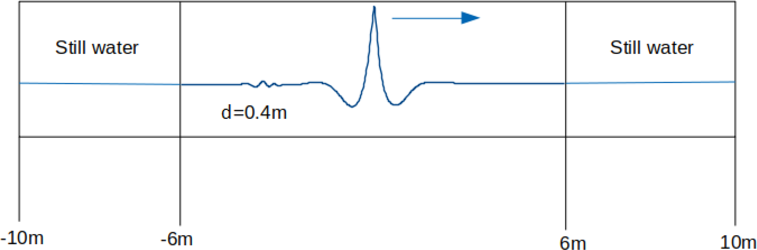
Numerical wave flume layout of the Lagrangian-OpenFOAM coupled model.
Table 1
| A, cm | Cases | -10 m to -6 m | -6 m to -4 m | -4 m to 4 m | 4 m to 10 m |
|---|---|---|---|---|---|
| 6.4 | peak-focussed GW (PFGW-BM1) | 20 60 | 25 60 | 800 60 | 30 60 |
| 6.8 | peak-focussed GW (PFGW-BM1) | 20 60 | 25 60 | 800 60 | 30 60 |
| 7.2 | peak-focussed GW (PFGW-BM1) | 20 60 | 25 60 | 800 60 | 30 60 |
| 7.2 | peak-focussed GW (PFGW-BM2) | 20 120 | 50 120 | 1600 120 | 30 120 |
Distribution of base mesh resolution for mesh resolution tests in different zones.
Notation: PFGW-BM is peak-focussed Gaussian wide spectrum - base mesh.
3.5 Geometric VOF coupled with adaptive mesh technique
To keep a smooth free surface in multi-phase flow, especially for rapid changes in curvature around wave crests, a novel geometric VOF technique called IsoAdvector in OpenFOAM is adopted. This technique has proven to be more efficient in preserving surface sharpness and suppressing excessive diffusion of the transport equation compared to the performance of the algebraic VOF method which employs the Multi-dimensional Universal Limiter for Explicit Solution (MULES) (Roenby et al., 2016, 2018; Larsen et al., 2018). It is noteworthy that the computational time can be approximately three times faster when utilising the geometric VOF method than using the algebraic VOF method. We found it efficient to obtain optimal results by combining the geometric VOF method with the adaptive mesh technique in OpenFOAM.
The fast changing breaking process around the wave crest requires sufficient mesh resolution, which is computationally expensive. To mitigate this, we employ adaptive mesh techniques to significantly reduce the number of grid nodes in the numerical domain. We employ the dynamicRefineFvMesh implemented in OpenFOAM, which utilises topological refinements of the mesh based on the volume fraction α. For each cell, octree cell refinement is triggered, dividing a hexahedral cell into eight sub-cells with 36 faces, of which 12 are internal to the master cell. The cells are automatically refined when the value of α falls within the range of 0.001 to 0.999, as specified by the user. Increasing the number of decimal places in the α value expands the area eligible for refinement. We set the refinement interval to approximately 0.0001 s, which is adequate for capturing fluid motion with less computational costs. For instance, if the time step is 10−5 s, the refine interval can be set to 10, resulting in a refinement time step of approximately 0.0001 s. The Adaptive Mesh Refinement (AMR) in OpenFOAM is currently only supported for hexahedral cells in 3D models. For this reason, we choose a pseudo-2D case, where a single layer is defined in the third direction with wall boundary conditions.
3.6 Boundary conditions
We apply standard OpenFOAM boundary conditions illustrated in Table 2. It is worth noting that the key distinction in boundary conditions between our work and other studies by different authors is that we use the more general boundary conditions rather than periodic boundary, which allows the breaking events to fully evolve without the effects of artificial boundary conditions. One potential artificial effect caused by periodic boundary conditions is the unnatural wave interaction. Waves that exit one side of the domain re-enter from the opposite side, leading to interactions that would not occur in a non-periodic setup. These interactions can influence wave breaking patterns, energy dissipation, and the overall vorticity field (Lubin and Glockner, 2015).
Table 2
| Type | Left | Right | Top | Bottom | FrontAndback |
|---|---|---|---|---|---|
| U | zeroGradient | zeroGradient | pressureInletOutletVelocity | slip | slip |
| p | zeroGradient | zeroGradient | TotalPressure | FixedFluxPressure | FixedFluxPressure |
| alpha.water | zeroGradient | zeroGradient | inletOutlet | zeroGradient | zeroGradient |
Boundary conditions for the coupled model.
We employ zeroGradient boundary condition at the inlet and outlet boundaries, which provides generic Neumann boundary conditions. This boundary condition implys that there is no change in the variable of interest across the boundary. It assumes that the boundary in our simulation is sufficiently distant from the region of interest to neglect its influence. Totalpressure boundary specifies p0 = 0 corresponding to the atmospheric pressure. On the bottom, front, and back walls, we apply the slip boundary condition, which assumes that fluid particles near the surface do not adhere to it. The more detailed description of boundary conditions used in the present work can be found in user manual OpenFOAM (2019).
3.7 Numerical settings
OpenFOAM provides various numerical schemes. The performance of these schemes can vary depending on the specific case and may require empirical testing for optimal performance. The combination of numerical schemes is listed in Table 3, which has proved to work well and yield good results. It is worth noting that the time schemes are critical for simulating wave propagation. The first-order Euler implicit time scheme can cause constant numerical diffusion, which leads to decreasing wave energy. The fully second-order Crank-Nicolson time scheme can overestimate the wave elevation. A coefficient in the OpenFOAM Crank-Nicolson time scheme provides a blending between Euler and Crank-Nicolson schemes and the value of 0.9 provides the highly effective performance for the numerical stability. Hence, we adopt this time scheme as our numerical time scheme.
Table 3
| Schemes | Term in OpenFOAM | Discretisation | Description |
|---|---|---|---|
| Time schemes | ddt | Crank-Nicolson time scheme | Second order, bounded, implicit |
| Gradient schemes | grad | Gauss linear | using Gauss’ theorem |
| Divergence schemes | div(rhoPhi,U) div(phi,alpha) div(phirb,alpha) | Gauss linearUpwindV, grad(U) Gauss vanLeer Gauss linear | Second order, Unbounded, upwind-biased Total variation diminishing (TVD) - |
| Laplacian schemes | Laplacian | Gauss linear corrected | interpolation scheme and snGrad scheme are required |
| Interpolation schemes | interpolation | linear | – |
| Surface-normal gradient schemes | snGrad | corrected | Linear with orthogonality correction |
| Wall distance calculation methods | wallDist | meshWave | Fast topological mesh-wave method |
Numerical schemes for the coupled model.
4 Mesh resolution and experimental validation
Mesh refinement tests were conducted to determine the adequate numerical resolution for our study. We present comparisons of surface profiles and the total energy profiles between different mesh resolutions using the coupled model with peak-focussed amplitudes: A = 6.4 cm, A = 6.8 cm, and A = 7.2 cm. Details of the numerical experiments are summarised Table 4, and the initial base mesh resolutions are provided in Table 1. For the cases utilising a static mesh, they are executed on 8 processors in parallel with 1.90 GHz for each core. The fixed time step used in these cases is 0.0001, and the maximum Courant number (Co) is set to 0.05. For the cases employing Adaptive Mesh Refinement (AMR), the parent cell is subdivided into 22 (level 2 in dynamicRefineFvMesh OpenFOAM utility) and 26 (level 3) sub cells around the surface as shown in Figure 2. The AMR results in the smallest mesh size of Δ = 1.25 mm with 1168 cells per wavelength for the cases with BM1-AMR level 3. For the case with BM2-AMR level 3, the smallest mesh size is Δ = 0.625 mm with 2336 cells per wavelength, which is comparable to the mesh resolution used in De Vita et al. (2018) with 2048 cells per wavelength. These simulations are run on the High Performance Computer (HPC) in the UCL cluster, utilising multiple processors with 2.5 GHz CPUs. The time step is set to be adjustable, with a maximum Courant number Co of 0.1. The exact time step varies between 5×10⁻⁵ - 6×10⁻⁵ s for the case with BM1-AMR level 3 and 2×10⁻⁵ - 3×10⁻⁵ s for the case with BM2-AMR level 3 in each numerical computation. The total simulation time is 4 s from −2 s to 2 s, which includes breaking events for breaking cases. Note that achieving strict convergence tests for weak breaking cases is challenging due to their sensitivity to numerical changes. It is important to assess mesh resolution effects against experimental data and examine energy evolution as wave breaking progresses.
Figure 2
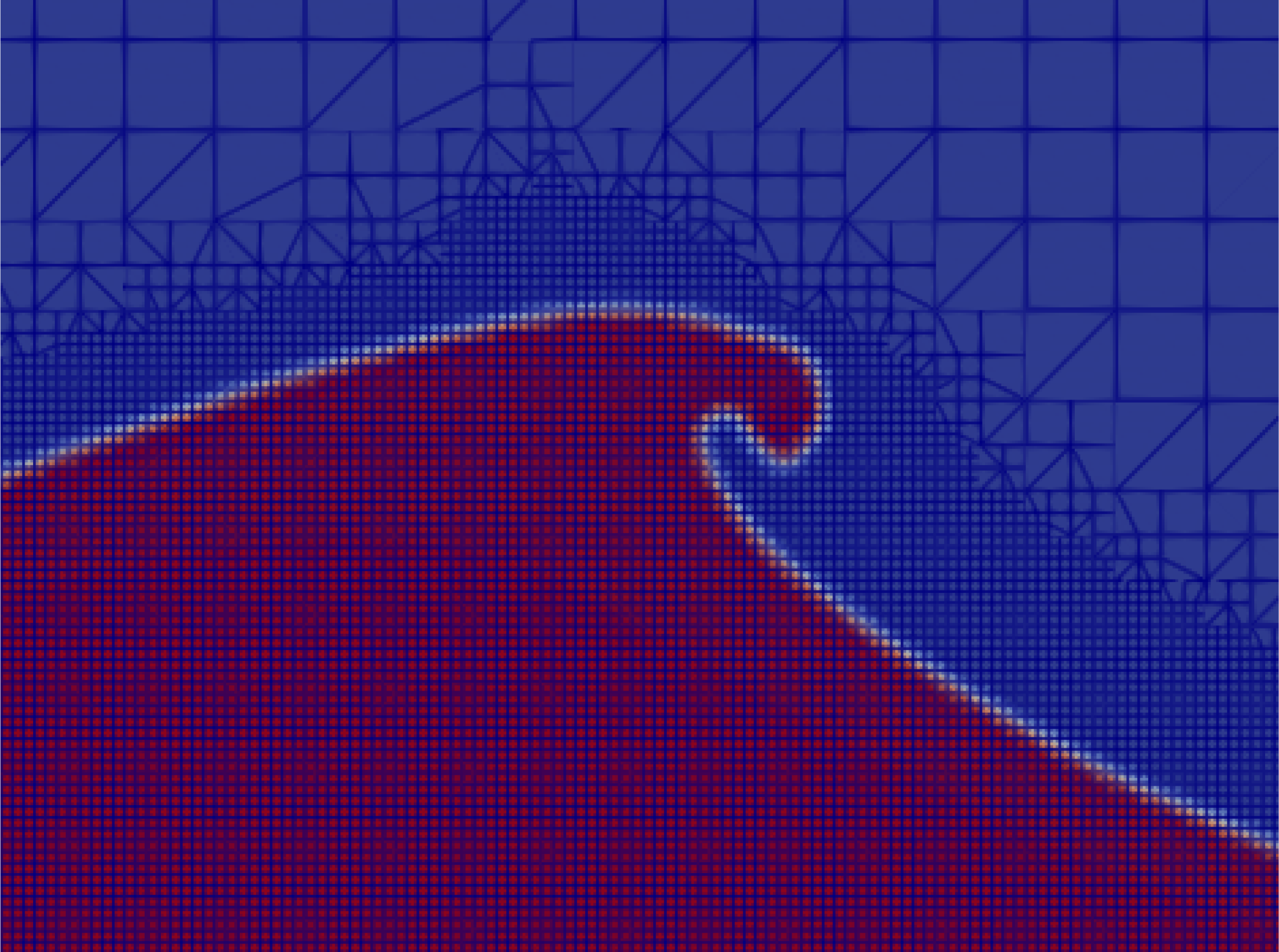
Snapshot of mesh refinement around the wave crest using Adaptive Mesh Refinement (AMR level 3).
Table 4
| A, cm | Cases | AMR refinement | Processor | CPU, day |
|---|---|---|---|---|
| 6.4 | 6.4 cm-PFGW-BM1-static mesh | – | 8 | 0.2 |
| 6.4 | 6.4 cm-PFGW-BM1-AMR level 2 | 22 | 60 | 0.1 |
| 6.4 | 6.4 cm-PFGW-BM1-AMR level 3 | 26 | 150 | 1.5 |
| 6.8 | 6.8 cm-PFGW-BM1-static mesh | – | 8 | 0.2 |
| 6.8 | 6.8 cm-PFGW-BM1-AMR level 2 | 22 | 60 | 0.11 |
| 6.8 | 6.8 cm-PFGW-BM1-AMR level 3 | 26 | 150 | 2.38 |
| 7.2 | 7.2 cm-PFGW-BM1-static mesh | – | 8 | 0.2 |
| 7.2 | 7.2 cm-PFGW-BM1-AMR level 2 | 22 | 60 | 0.15 |
| 7.2 | 7.2 cm-PFGW-BM1-AMR level 3 | 26 | 150 | 3.3 |
| 7.2 | 7.2 cm-PFGW-BM2-AMR level 3 | 26 | 200 | 40 |
Numerical cases with the no turbulence model for mesh resolution tests of the coupled model.
The OpenFOAM simulations were run for 4 s (from −2 s to 2 s).
To quantify energy dissipation, the kinetic energy Ek is calculated by numerically integrating over the entire water domain, and the potential energy component Ep is obtained through the integration of the potential energy density on a free surface.
The expression of potential energy is
where η is the surface elevation (deviation from the mean water level).
The expression of kinetic energy is
Hence, the total energy is
In our study, we neglect the potential energy associated with surface tension due to its minor contribution to the total wave energy, especially in cases characterised by high Bond number (the ratio of gravity to surface tension). It is important to note that when calculating potential energy in cases involving air bubbles or splashes, we follow these procedures: for each data node on the surface, if there exists an air void beneath the free surface, we calculate the potential energy using the adjusted surface elevation, which is the surface elevation minus the air void length; if there is a splash above the free surface, we calculate the potential energy using the adjusted surface elevation, which is the surface elevation plus the length of the splash. Kinetic energy is computed through numerical integration over all cells within the entire water domain containing water (α ≥ 0.05). The error in total energy estimation is then determined by the mesh resolution near the surface. The method employed for calculating total energy yields a negligible numerical error, typically less than 0.1%, when compared to the theoretical total energy for the nonbreaking case based on the 1st order Stokes wave theory (in our preliminary study, not shown in this paper).
We compared surface elevations generated by the Lagrangian model with those produced by the coupled model using different resolutions at four time instances: t = −1 s, 0 s, 1 s, and 2 s presented in Figure 3. The surface profiles generated by the Lagrangian model are depicted in black and are presented as references. As expected, the non-breaking case converges rapidly due to the absence of turbulence. The surface elevation modelled by the coupling model with a static mesh (grey line) exhibits the lowest level of accuracy compared to cases with higher resolutions. In particular, the maximum height of wave crest is overestimated at the focussed point at t = 0 s, as shown in the top right panel of Figure 1. By increasing the resolution through the application of AMR, the cells around the free surface are refined into 22 (level 2), providing a sufficient mesh resolution to accurately estimate the wave crest height, as depicted in the zoomed-in subplot. The surface profiles with AMR refinement (blue and red lines) closely match the surface profiles obtained by the Lagrangian model everywhere else except the disparities on the left side of the domain. The differences are due to the fact that we use coarser mesh resolutions away from the central domain of -10 m to -4 m, which is out of the central region where the main wave crest travels. The parts of wave components which travel in the left side of the domain do not affect the main crest of the wave that travels faster than them.
Figure 3
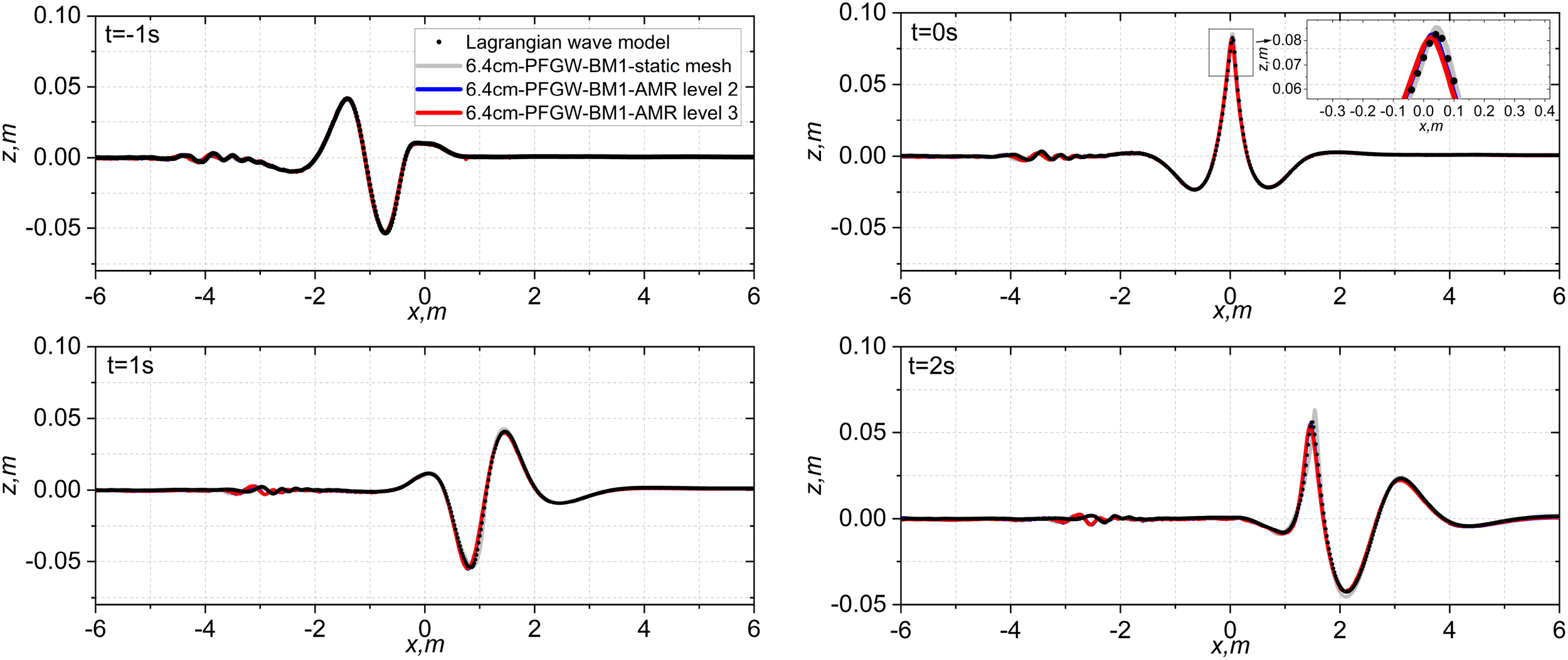
Comparison of the surface elevation between the surface elevation produced by the Lagrangian model and the surface elevation obtained by the coupled model at t = −1 s,0 s,1 s and 2 s for the peak-focussed GW wave groups with A = 6.4 cm (non-breaking) for different mesh resolutions.
Figure 4 illustrates comparisons of wave profiles for cases of weak and strong breaking with different mesh resolutions. These figures present comparisons of the overall free surface evolution and zoomed-in wave crest views for different resolutions, with results from the Lagrangian wave model serving as reference data.
Figure 4
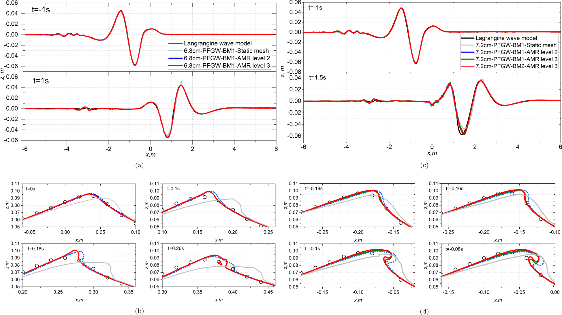
Comparison of the surface elevation between the surface elevation produced by the Lagrangian model and the surface elevation obtained by the coupled model for the peak-focussed GW wave groups: (a) Comparisons of surface evaluation from −6 m to 6 m along the flume at t = −1 s and t = 1 s for Wave groups with A = 6.8 cm. (b) Breaking wave crest between t = 0 s and t = 0.26 s for Wave groups with A = 6.8 cm. Lagrangian model (white circle). The coupled model: Static mesh (grey line); BM1-AMR level 2 (dot blue); BM1-AMR level 3 (dot red). (Part 1). Comparison of the surface elevation between the surface elevation produced by the Lagrangian model and the surface elevation obtained by the coupled model for the peak-focussed GW wave groups: (c) Comparisons of surface evaluation from -6 m to 6 m along the flume at t = −1 s and t = 1.5 s for Wave groups with A = 7.2 cm. (d) Breaking wave crest between t = −0.18 s and t = −0.08 s for Wave groups with A = 7.2 cm. Lagrangian model (white circle). The coupled model: Static mesh (grey line); BM1-AMR level 2 (dot blue); BM1-AMR level 3 (dot green); BM2-AMR level 3 (dot red). (Part 2).
In the case of weak breaking, a satisfactory agreement is observed for the modelled free surface with various mesh resolutions at times t = −1 s and t = 1 s, as demonstrated in Figure 4a. Only the lowest resolution exhibits a poor prediction without capturing the formation of overturning, while the results obtained from higher resolutions using the coupled model achieve good agreement with the crest profiles from the Lagrangian model prior to breaking onset, e.g. comparison of the wave crests at t = 0 s shown in Figure 4b. In general, the weak breaking occurs for a short period of time within a small area around the crest, and then the wave group will continue to move steadily along the flume after the completion of energy dissipation due to breakers. Consequently, the amount of total energy dissipated by breakers can be correctly calculated if the pre-breaking state and post-breaking steady state of wave groups are well predicted. The findings shown in Figure 4a give us confidence that further calculations related to energy dissipation from weak breakers can yield accurate results. It is worthy noting that the Lagrangian wave model applies a treatment of breaking to suppress the overturning of wave crest, resulting in good predictions for the pre-breaking state and reasonable overall predictions for post-breaking state. After the completion of wave dissipation due to breaker, the surface modelled by the coupled model continues to closely match the one produced by the Lagrangian wave model, which might indicate that both models simulate similar overall energy dissipation process in the breaking length and time scales. Comparisons of breaking crest between t = 0 s and t = 0.26 s are shown in Figure 4b, where the white circle is the crest obtained by the Lagrangian model and the others are from the coupled model. We can observe that the wave crests calculated by the coupled model are captured correctly in the wave phase, which is consistent with the prediction by the Lagrangian wave model. Again, the lowest resolution fails to correctly predict the onset of breaking which is defined as the instant when the front crest face becomes vertical. In contrast, the breaking crests obtained by the coupled model with higher resolutions closely match the predicted onset of breaking by the Lagrangian model. At t = 0 s, the wave crests from both models almost perfectly overlap. The main difference lies in the detailed motion of the upper part of the wave crests during breaking after t = 0 s. The simulation of wave crest by the coupled model with the VOF method presents the overturning, air entrapment and subsequent processes due to breakers. The resolved crest with the resolution AMR level 2 (blue dot) forms a vertical front face and overturns along the underneath front surface without the air entrapment, whereas the simulated top part of crest with the resolution AMR level 3 (red dot) forms a steeper vertical front face at t = 0.18 s and then overturns and traps a very small volume of air. The highest resolution test simulates a more detailed deformation of the wave crest during the evolution of breaking waves overturning. Since the breaking intensity by weak breakers is very mild and the deformation of weak breaking crest only occurs in a compact region around the wave crest, we anticipate that further increasing the resolution for the weak breaking cases would yield numerical results with subtle differences compared to the test with the resolution BM1-AMR level 3. Therefore, we consider the resolution BM1-AMR level 3 sufficient to correctly represent the geometric deformation of wave crests for weak breaking cases at affordable computational costs.
In respect of the strong breaking case, Figure 4c shows the surface profiles with all resolutions overlap each other at early time t = −1 s before breaking as expected. However, after the occurrence of intense turbulence due to breakers, the surface profiles appear slight discrepancies for different wave models and different mesh resolutions at time t = 1.5 s. At time t = 1.5 s, it can be seen that the surface profiles at the trough obtained by the coupled model shift slightly forward compared with the trough simulated by the Lagrangian model, but the rest parts of the surface profile are in line with each other. Again, the test with the static mesh reproduces the most inaccurate surface profiles around the crest and trough. More details of breaking crests prior and after the onset of breaking are depicted in the bottom panel of Figure 4d from −0.18 s to −0.08 s. Similar to the comparison for the weak breaking tests, the wave phases of strong breaking cases simulated by two wave models are consistent and differences can only be observed at the tops of the wave crests at the breaking. Generally, the tests with the resolutions of BM1-AMR level 3 (green dot) and BM2-AMR level 3 (red dot) represents geometric formations of breaking crest that are very close to each other, whereas the numerical tests with lower resolutions exhibit flatter front face of breaking crest. One noticeable difference we can see is that the simulation with higher resolution forms a sharper forward jet during the overturning process. This is because a higher density of numerical points around the wave crest can represent a higher curvature of the overturning wave crest and a coarser mesh resolution can filter out the detailed feature of the curvature of breaking crest. From the demonstration of the zoom-in wave crest, a sufficient mesh resolution around the wave crest is critical. Static mesh tends to reproduce inaccurate detailed deformation of wave crest unless the extreme high density of resolution is applied around the breaking crest. On the contrary, AMR technique can refine the cells around the surface of wave crest and then provides more accurate information in the vicinity of breaking crest.
The normalised total energy profiles for the non-breaking case are shown in the left panel of Figure 5. The evolution of total energy exhibits a non-physical increase of approximately 12% due to insufficient mesh resolution near the surface, which leads to spurious velocities at the interface and an overestimation of wave heights when using the static mesh. With AMR applied, the other two curves demonstrate improved energy conservation for tests with AMR level 2 and level 3, where the total energy remains constant from t/Tp= −1.8 to t/Tp= 2. This is consistent with the fact that there are no breaking or other processes leading to significant change of energy within the water phase in the numerical domain. Note that the total energy is normalised by the selected initial total wave energy calculated at t/Tp= −1.8. We use the value of total energy at t/Tp= −1.8 as the initial time to calculate the total energy rather than the actual simulation start time at t/Tp= −2. The transition of cells from a static mesh to an adaptive mesh during the refinement process takes a short time approximately 0.2 s to reach stable state. Hence, we choose t/Tp= −1.8 as the initial moment for calculating the total energy so as to reduce the errors caused by the refinement of cells.
Figure 5
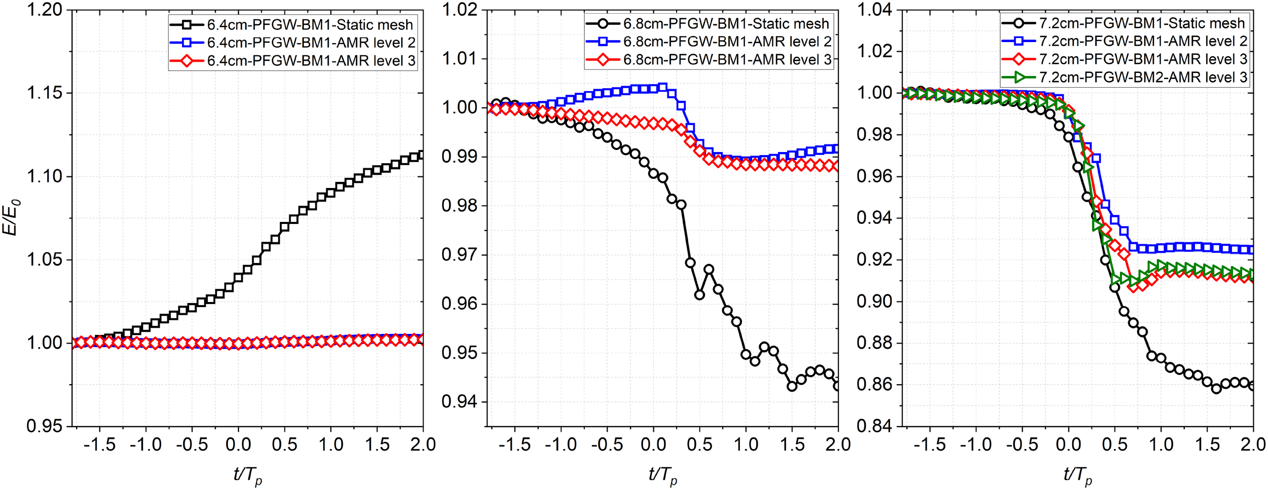
Convergence of the normalised total energy profiles for the peak-focussed GW wave groups for the cases with the no turbulence model, where Tp is the peak frequency. Left panel: A = 6.4 cm (non-breaking); Middle: A = 6.8 cm (weak breaking); Right panel: A = 7.2 cm (strong breaking).
The evolution of total energy for weak breaking cases is presented in the middle panel of Figure 5. The total energy dissipation significantly decreases with each refinement of mesh resolution. The case with the lowest resolution exhibits the most substantial energy jump, and the evolution of total energy displays fluctuations over time after the onset of breaking. However, the case with AMR level 2 resolution shows a non-physical trend where total energy increases with time both before and after breaking. Only the case with AMR level 3 resolution accurately represents the trend in total energy dissipation. In this case, total energy slightly decreases before the onset of breaking and then experiences a noticeable jump during the wave dissipation due to breakers. Subsequently, after the active breaking stages, the total energy returns to its normal pattern with a slight overall decrease over time. Although the energy dissipation is relatively small, approximately 1.12%, from t/TP= −1.8 to t/Tp= 2, the total energy profile indeed exhibits an energy jump during the active breaking phase.
For the strong breaking case shown in the right panel of Figure 5, the total energy calculation for the strong breaking cases is less sensitive to numerical errors compared to the weak breaking case, where the total energy exhibits a smooth and gradual decay when no turbulence is present. The tests with static mesh (black) and BM1-AMR level 2 (blue) respectively underestimate and overestimate the total energy dissipation due to wave breaking. Conversely, the results for the other two higher resolutions (red and green) indicate a similar amount of wave energy dissipation during the active breaking phase. These two curves closely match up to t/Tp= 0.2, after which a discrepancy emerges and gradually widens during the later part of the active breaking phase. However, after the completion of wave energy dissipation, these two curves return to a similar level of energy balance. The discrepancy between the two curves from t/Tp= 0.4 to t/Tp= 0.7 is attributed to the finer mesh resolution modelling smaller bubbles, droplets, and additional detail on chaotic turbulence after the wave crest reenters the water surface, compared to the lower mesh resolution. Achieving full convergence for the strong breaking cases is challenging and reliant on computational speed capability. The difference between the tests with different resolutions during the later stages of the active breaking phase is expected and may persist even with further mesh refinement. Yet, the overall energy decay rate for the two higher resolutions is of the same order, yielding 0.12629 and 0.12633 respectively, as determined by linear fitting. When the mesh resolution is refined to a certain level, the energy dissipation rate becomes independent of or only minimally affected by the mesh resolution, although the instantaneous dissipation rate may show relatively larger differences. This observation is consistent with conclusions drawn in existing studies investigating energy dissipation rates due to breakers (Deike et al., 2016; De Vita et al., 2018). Consequently, we consider the result with the mesh resolution BM1-AMR level 3 to be acceptable and suitable for systematically studying the evolution of energy dissipation in strong breaking cases at an affordable computational cost.
To further validate the coupled wave model, comparisons between experimental time histories of surface elevations, experimental spatial wave profiles, and modelled surface profiles are presented.
Experimental time histories were taken using probes at six different positions for all tests: x = 0 m, 0.5 m, 1 m, 1.5 m, 2 m, and 2.5 m, as depicted in Figure 6. We evaluate the deviations between the experimental and modelled spectral components of the surface elevation using the root mean square error (RMSE) formula:
Figure 6
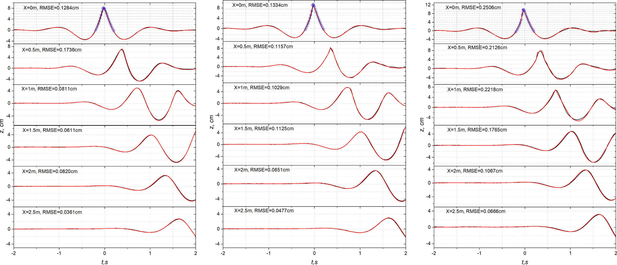
Comparison of time histories of surface elevation between the measured surface elevation and the surface elevation obtained by the coupled model at different positions alone the flume for the peak-focussed GW wave groups with A = 6.4 cm (left), A = 6.8 cm (middle), A = 7.2 cm (right), at locations x = 0 m, 0.5 m, 1 m, 1.5 m, 2 m and 2.5 m. The black line: Experimental measurements; The red line: Numerical results obtained by the coupled model with the no turbulence model; The blue circle: Numerical results obtained by the Lagrangian model.
where zci and zmi are the discrete spectral components calculated by the coupled model, and measured in the experiments, respectively, in the range [0,…,161] with N = 161.
For the non-breaking case depicted in the left panel of Figure 6, comparisons of surface elevation over time between the measured surface elevation and the modelled elevation show equal accuracy for all selected probes. The main wave crests are accurately predicted by the coupled model in comparison to the measured main wave crests at the locations x = 0, 1, 1.5, 2, 2.5 m except the slightly larger discrepancy at x = 0.5 m. The overall deviations are even smaller for the gauges located farther away from the midpoint of the flume. The result from the Lagrangian model (blue circle) at x = 0 is demonstrated as references. It is evident that the modelled time histories of surface elevation exhibit a very satisfactory agreement with the experimental results for the non-breaking case.
The time histories of surface elevation for the peak-focussed weak and strong breaking groups between numerical and experimental tests are shown in the middle and right panels of Figure 6, respectively. In both cases, the numerical results obtained using the coupled model with the selected mesh resolution (BM1-AMR level 3) closely align with the results from the Lagrangian wave model at the probe located at x = 0 m. The maximum surface elevations calculated by the two models are in excellent agreement. This demonstrates the effectiveness of the coupled method in replicating the surface elevation from the Lagrangian wave model to the VOF model, particularly around the focussed point. The level of accuracy for the weak breaking case is comparable to that of the non-breaking case. As expected, the discrepancies for the cases with higher amplitudes become larger than non-breaking cases. The increasing difference may be attributed to factors mentioned in Section 5, Buldakov et al. (2019) where they pointed out that the recorded crest elevation is lower than the actual crest elevation for very steep wave peaks due to a cavity around the wires of the wave probe caused by the high-speed flow at the crest. The evidence can be observed from the top graph in Figure 6 that the measured time histories at x = 0 m shows more symmetric than the ones modelled by the numerical models for high steep waves. In common sense, as expected, the steeper wave peaks may exhibit more asymmetric characteristics close to the scenario simulated by the numerical models.
Table 5 summarises the RMSE between the experimental and modelled surface elevation corresponding to cases shown in Figure 6. The RMSE values for non-breaking case result in smallest values compared to the cases with higher wave amplitudes at most selected locations. Notably, the RMSE at the probe x = 0.5 m for the weak breaking test is even smaller than that for the non-breaking test. However, there is a discrepancy in the maximum surface elevation simulated by the numerical models around the focussed point compared to the laboratory measurements. In general, the RMSE values for the stronger breaking cases are slightly larger than those for the weaker breaking cases, and the discrepancies tend to decrease as the probes move away from the central point of the flume. Noticeable differences primarily occur around the main trough and crest of the wave group at the locations of the first three probes and become less pronounced at the locations of the downstream probes. The variations in RMSE values at various recording locations reflect consistency with the factors reported in Section 5, Buldakov et al. (2019) as we also mentioned above. When the probe is situated in areas without breaking, recording precise surface elevation in the physical flume is more reliable. However, obtaining accurate surface elevation becomes challenging in locations with turbulence. Overall, the comparisons between the experimental results and the numerical results demonstrate good agreement.
Table 5
| A, cm | Parameter | x =0 m | x =0.5 m | x =1 m | x =1.5 m | x =2 m | x =2.5 m |
|---|---|---|---|---|---|---|---|
| 6.4 | Free surface elevations (cm) | 0.1284 | 0.1736 | 0.0811 | 0.0611 | 0.0820 | 0.0361 |
| 6.8 | Free surface elevations (cm) | 0.1334 | 0.1157 | 0.1029 | 0.1125 | 0.0851 | 0.0477 |
| 7.2 | Free surface elevations (cm) | 0.2506 | 0.2126 | 0.2218 | 0.1765 | 0.1087 | 0.0666 |
Summary of Root-Mean-Square Error (RMSE) between the experimental and modelled surface elevation corresponding to cases shown in Figure 6.
Comparison of spatial wave profiles at selected instants for the strong peak-focussed waves with A = 7.2 cm is illustrated in Figure 7. Wave crest extraction was conducted in a 1.1 m × 0.4 m view frame recorded by a centrally positioned high-speed camera in the flume. The left column of Figure 7 shows numerical results compared with digitised experimental surface profiles obtained via a post-smoothing method, neglecting crest overturning considerations. The right column presents direct comparisons between numerical results and snapshots of wave surface profiles captured by the high-speed camera. Upon close observation, these comparisons reveal high consistency, particularly evident in the outer profiles visible in the right column of Figure 7. The modelled phase of wave groups aligns well with experimental measurements. At t = −0.4 s, the comparison of wave surface profiles shows high consistency during the early stages of wave propagation towards breaking. However, as waves approach breaking, discrepancies emerge around small wave crest areas and become more pronounced over time. The experimental waves exhibit slight earlier breaking and a different breaking type compared to simulations (the videos by the camera do not show crest overturning; however, observations under a laser sheet cached the crest overturning for the same case). This discrepancy may be attributed to (i) 3D crest instability and (ii) destabilising effects of the walls, which generate small waves near the wall as the crest propagates (observed from the top-view images of the wave crest propagation in the transverse direction). Recorded videos and digitised data illustrate occurrences at the contact line with the glass wall, potentially differing from events at the flume centerline. Despite these considerations, our numerical results consistently demonstrate good agreement with experimental measurements.
Figure 7
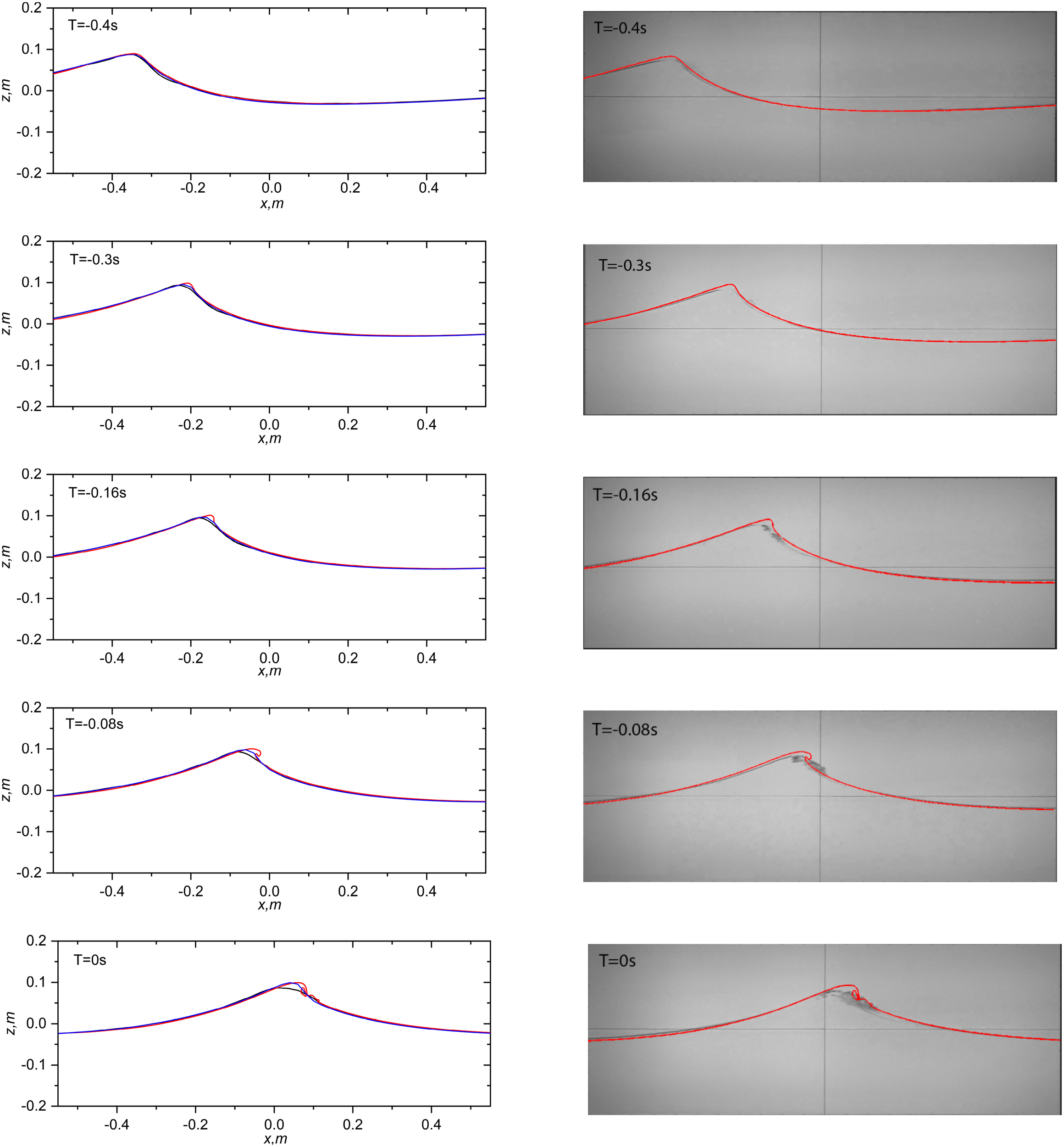
Comparison of spatial wave profiles between numerical results and experimental measurements for the strong peak-focussed waves with A = 7.2 cm. Left column: Comparisons of numerical results and digitised experimental surface profiles from x = −0.55 m to x = 0.55 m. Right column: Comparisons of numerical results and snapshots of wave surface profiles recorded by the high-speed camera. The aspect ratio for each figure is consistent. Red curve: Modelled surface obtained from the coupled model without turbulence models. Blue curve: Numerical results obtained from the Lagrangian wave model. Black curve: Experimental results.
In conclusion, we validate and evaluate the coupled model with respect to surface profiles, the evolution of total energy at different mesh resolutions, and comparisons of time histories of surface elevations and spatial surface profiles between the selected numerical tests and the experimental measurements. Achieving a true DNS simulation for post-breaking processes, which involve turbulence and the generation of small bubbles and droplets, requires exceedingly large computational resources. Even the highest resolution computation (BM2-AMR level 3) presented in Table 4 is already considered impractical, requiring over 40 days of computation time (excluding queue time on the cluster system). For the weak and strong breaking cases, conducting 2D simulations is not suitable for investigating the distribution of bubbles and droplets due to wave breaking. Our primary focus is on studying the different evolution in the vicinity of the wave crests associated with various breaking scenarios using predefined spectra. Therefore, achieving full convergence in these studies may not be critical. Consequently, the selected mesh resolution (BM1-AMR level 3) is considered the appropriate one for modelling the wave breaking cases with good accuracy and affordable computational costs. Each run takes approximately 2–3 days, making it practical for a systematic study of extensive cases. The mesh resolution we select is considered valid for our interests in studying the evolution of breaking wave crests up to the phase when wave crests reentry to the water surface and also the overall wave energy dissipation due to breakers.
5 Results and discussion
In the subsequent two subsections, we present the peak-focussed GW wave groups with four different turbulence models for the weak and strong breaking cases. All tests are simulated with the mesh resolution BM1-AMR level 3. The computational time for the LES Smagorinsky model and LES k-equation model is approximately 20% and 60%, respectively, of the computational time for the cases without a turbulence model indicated in Table 4. For the RANS standard k − ϵ and RNG k −ϵ models, the computational time is about 50% of the computational time for the cases without a turbulence model. To assess the effects of turbulence modelling on wave breaking processes, the wave crests with and without turbulence models at onset of breaking are presented along with the comparisons of crest profiles. Comparisons of time histories of breaking crests are demonstrated. Detailed comparisons of the wave crests between the numerical and experimental results are also presented. The total energy profiles obtained by the coupling method with different turbulence models are examined and the variations on the dimensionless breaking b for the cases with different turbulence models are calculated.
5.1 The effects of turbulence models on prediction of breaking surface profiles
Figure 8 illustrates the predicted time and the wave crest at the moment of breaking onset with and without turbulence models. As can be seen from the left panel of Figure 8a, the results obtained by LES simulations (red and blue) predict the time of breaking onset t = 0.16 s, which is ahead of t = 0.18 s predicted without turbulence models (black). The test with RANS RNG k − ϵ model (purple) gives the predictions of the time of breaking onset at t = 0.23 s which is delayed by 0.5 s compared to the one predicted without turbulence models. The test with RANS standard k − ϵ model only shows a maximum wave height at t = 0.16 s. This wave group does not form a vertical crest front face and there is no occurrence of breaking beyond the time of formation of maximum wave height. In this case, the test with RANS standard k − ϵ model does not correctly capture the breaking features for the weak breaking case. However, the improved RNG k − ϵ model that takes into account more turbulence scales represents the similar behaviour of the evolution of breaking wave crest. The maximum wave heights for the tests with LES turbulence models and without turbulence models are very close to each other and the maximum wave heights predicted by LES turbulence models is just slightly larger than the one predicted by the test without turbulence model. The RNG turbulence model results in a lower maximum wave height at the breaking onset. In contrast, the right panel of Figure 8a demonstrates that the strong breaking cases are less sensitive to the application of turbulence models. All tests represent the formation of vertical front faces and the simulated time of breaking onset are close to each other within the difference of 0.02 s except the test with RANS standard k − ϵ model which predicts the breaking onset delayed by around 0.6 s compared to the one predicted without turbulence models.
Figure 8
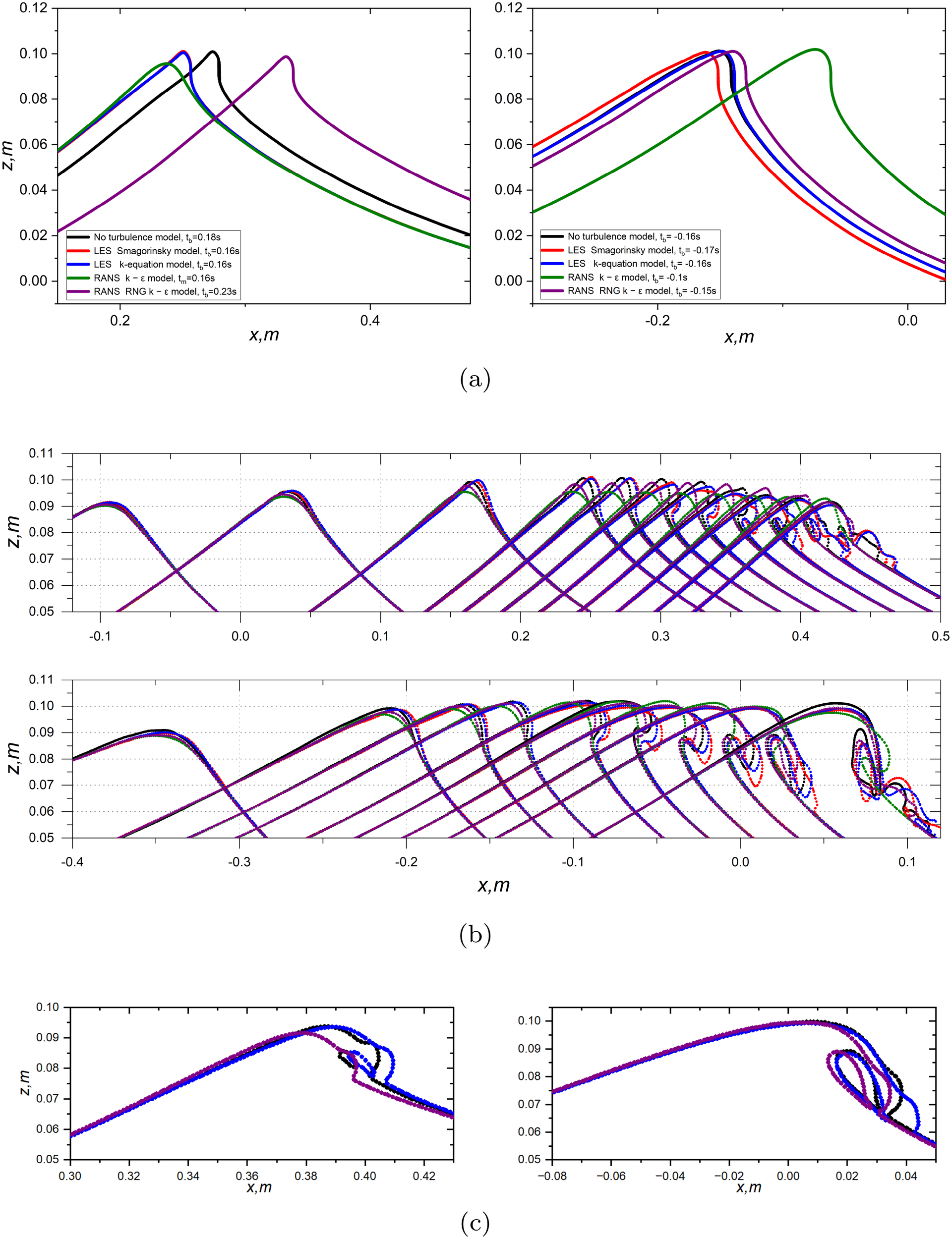
Comparisons of wave crest of the breaking onset with and without turbulence models. Waves propagate from left to right: (a) Wave crest at breaking onset. Left panel: Wave crests with A = 6.8 cm (weak breaking) except the case with RANS standard k − ϵ model (no breaking occurrence); right panel: Wave crests with A = 7.2 cm (strong breaking). (b) Evolution of surface profiles over time. Top panel: Wave crests with A = 6.8 cm (weak breaking), wave profiles at t = −0.1, 0, 0.1, 0.16, 0.18, 0.2, 0.22, 0.24, 0.26, 0.28 and 0.3 s; Bottom panel: Wave crests with A = 7.2 cm, wave profiles at t = −0.3, -0.2, -0.17, -0.15, -0.12, -0.1, -0.08, -0.06, -0.04, and 0 s. (c) Zoom-in crest profiles at the instant when the overturning jet initially touches the underlying water surface. Left panel: Case with A = 6.8 cm; Right panel: Case with A = 7.2 cm. The different colours in (b, c) present the same cases shown in (a). Note that the wave phases have been shifted to align the profiles for better comparison across the selected cases.
Figure 8b illustrates the deformation of breaking wave crests between the cases with and without turbulence models. The differences between different cases appear around the breaking crests. The evolution of breaking crest show the time difference of breaking onset. It is qualitatively similar in shape of breaking but the volume of air entrapment is different. The cases with LES turbulence models exhibit breaking with a more substantial air pocket beneath the breaking jet, whereas simulations employing RANS turbulence models represents smaller volume of air entrapment as shown in Figure 8c. Note that the wave phases have been shifted to align the profiles for better comparison across the selected cases. These observations are consistent with the intensities of energy dissipation due to breaking discussed in the following sections.
Figure 9 shows the comparison of time histories for the wave crests obtained by the tests with different turbulence models (coloured lines) and the experimental results (grey circles). Negligible differences are observed for the selected location x = 0 m for the test with and without turbulence models in both weak and strong breaking cases. For the wave groups with A = 6.8 cm, the test with LES k-equation model exhibits the best performance as the simulated profile (blue line) is close to the experimental results. However, substantial discrepancies emerge for wave groups with A = 7.2 cm. This discrepancy may arise from the methodology employed to calculate actual surface elevations in numerical simulations. In our approach, simulated elevations are computed by excluding the length of the air bubble at the selected positions. Consequently, simulated surface elevations may be smaller than the measured counterparts which might not exclude the part of air underneath. Exclusively focussing on the comparison of surface profiles of wave crests may not fully capture the performance of wave models. One evidence is that we notice the simulated time history profile obtained using the RANS k − ϵ model (green line) closely matches the experimental measurements, but there is no air bubble simulated underneath the surface at the location x = 0.5 m from t = 0.3 s to t = 0.4 s. This implies that a comprehensive assessment of wave model performance should integrate surface profiles with considerations of energy dissipation. Such an approach is expected to yield more robust and reliable conclusions.
Figure 9
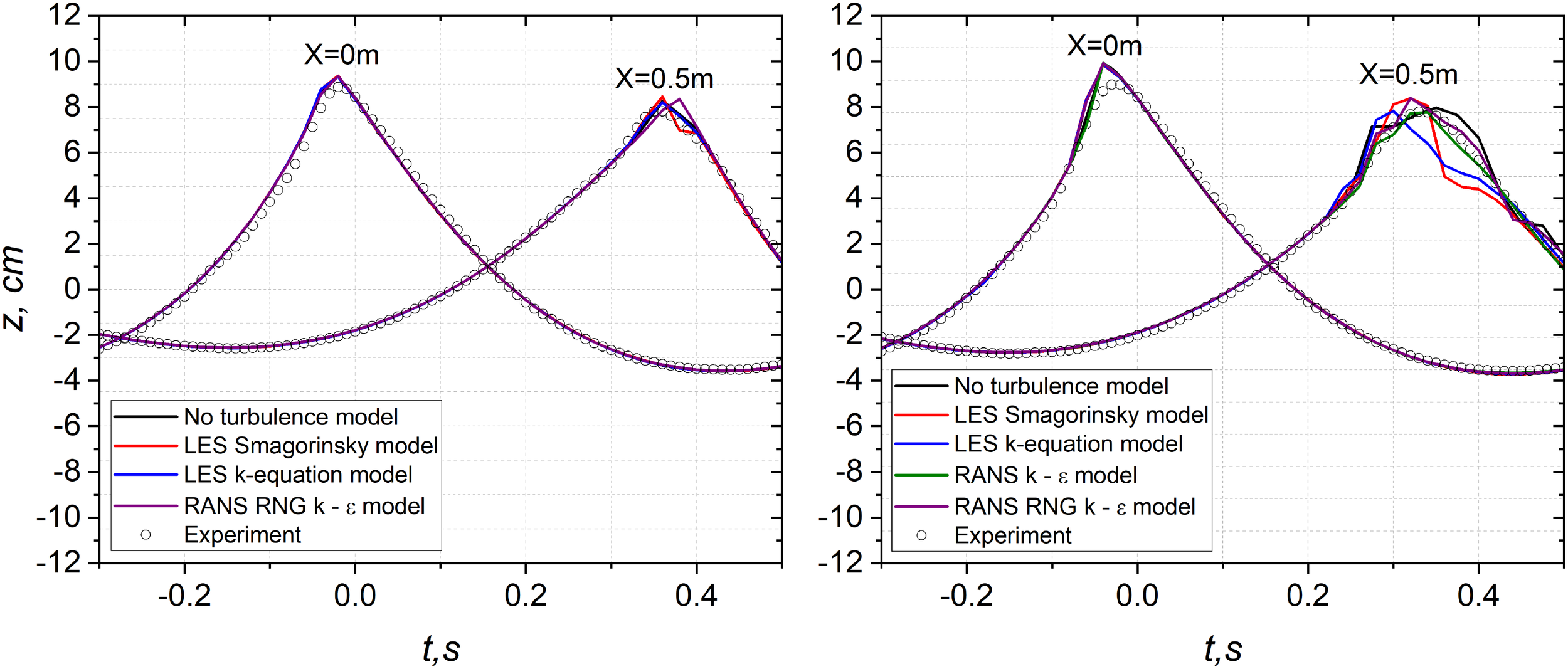
Comparison of time histories of wave crest between the measured surface elevation and the surface elevation obtained by the coupled model with and without turbulence models at x = 0, 0.5 m. Left panel: Wave groups with A = 6.8 cm (weak breaking); Right panel: Wave groups with A = 7.2 cm (strong breaking).
To further evaluate the accuracy of the modelled wave crests obtained using different turbulence models, we compare them with experimentally measured wave crests captured under a laser sheet for the peak-focussed case with A = 7.2 cm (strong breaking case) from Chasapis Tassinis (2023). The comparison is conducted at three time instants, starting from the onset of wave breaking, with a 0.01 s interval. Due to differences in spatial and temporal coordinate systems between the numerical simulations with and without different turbulence models and experimental measurements, specifically horizontal shifts of approximately 5.5 cm to 14 cm and variations in time references, direct comparison is not straightforward. To ensure a meaningful comparison, we first identify a common reference point, defined as the moment when the front face of the wave becomes vertical at the onset of breaking in both datasets. Using this reference, experimental wave profiles are extracted at 0.01 s intervals for direct comparison. Furthermore, the horizontal coordinates of the numerical results are shifted based on deviations observed at the lowest available data points in the experimental dataset. These adjustments improve the alignment between numerical and experimental results, allowing for better comparisons of the performance of different turbulence models in capturing breaking wave crest shape.
Figure 10 presents a comparison of wave crests between numerical simulations with and without turbulence models and experimental measurements. The overall curvature of the wave crest front face in different simulations closely follows experimental observations, likely due to the accurate initial wave conditions before breaking, generated by the Lagrangian wave model. However, differences emerge between simulations employing different turbulence models. Simulations using LES turbulence models show better agreement with experiments, as the wave crest and lower front face align more closely with the measurements. The LES k-equation turbulence model provides the closest crest profiles with the least deviation. The simulation without a turbulence model also produces relatively accurate surface profiles, but the front face curvature is slightly smaller, and the upper body of water inclines slightly backward compared to the experimental benchmark. The RANS k − ϵ turbulence model exhibits the largest deviations from the experimental profiles, with the flattest front face curvature, whereas the RNG k −ϵ turbulence model demonstrates improved performance compared to the standard RANS k − ϵ model. These variations in breaking crest evolution can be interpreted in conjunction with the total energy evolution simulated by different turbulence models, highlighting one of the most significant findings of this study. This aspect is further explained in the following section.
Figure 10
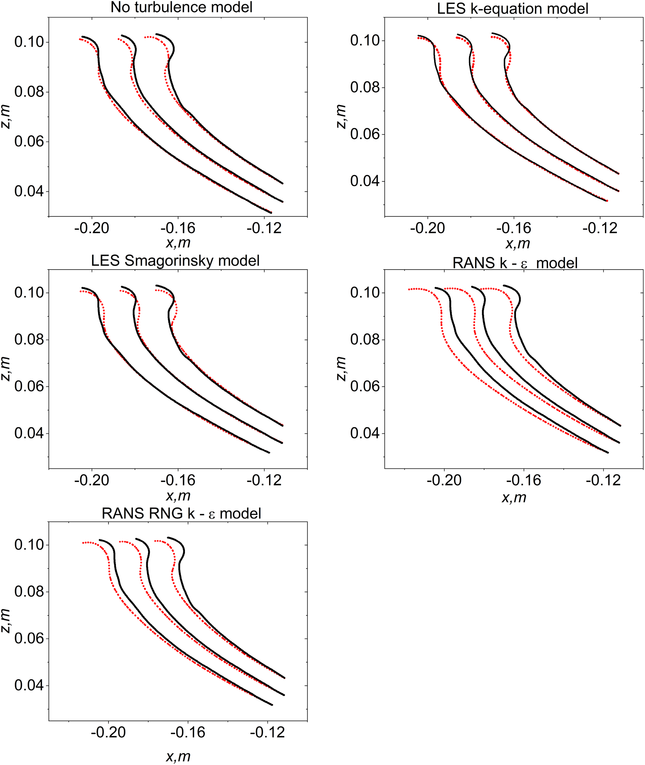
Comparison of breaking wave crests between experimental measurements (black line) and numerical results (red dots) obtained using the coupled model with and without turbulence models at three time instants. A horizontal coordinate shift is applied. The first instant corresponds to the moment when the front face of the wave becomes vertical at the onset of breaking, followed by intervals of 0.01 s.
5.2 The effects of turbulence models on the energy dissipation due to breakers
The normalised total energy dissipation and two wave energy components for the peak-focussed GW wave groups both with and without turbulence models is presented in Figure 11. For the weak breaking cases shown in the left panel of Figure 11a, tests utilising LES turbulence models and the RNG k − ϵ model exhibit similar energy dissipation behaviours due to breaking compared to simulations conducted without turbulence models. The test with standard k−ϵ model demonstrates a continual decrease in total energy and there is no obvious energy jump due to the absence of breaking. The LES simulations result in the highest energy dissipation due to breaking, dissipating approximately 1.2% of total energy during the active breaking phase from t/Tp= 0.2 to t/Tp= 0.7 for both tests utilising LES turbulence models. The tests with the RNG k−ϵ model and without turbulence models display smaller percentages of energy dissipation, around 0.6% between t/Tp= 0.3 and t/Tp= 0.7, and 0.8% between t/Tp= 0.2 and t/Tp= 0.7 during the active breaking stage, respectively. Such small percentages of total energy dissipation are difficult to be measured in physical tests due to the sensitivity and uncertainties. Only few authors have reported values close to a few percent in their findings as we noticed so far. Banner and Peirson (2007) computed a total energy loss of approximately 2.1% for their marginal breaking case using the control volume approach to estimate energy loss due to breakers induced by modulational instabilities. More recently, following the similar method for estimating the energy loss, Craciunescu and Christou (2020) investigated wave breaking energy dissipation for dispersive focussed wave groups based on JONSWAP spectra, reporting the smallest energy dissipation due to breakers at around 1.3% for the weakest breaking cases based on measurements between two wave gauges located far from the centre of the wave tank. Our results for the weak breaking cases qualitatively align with these previous findings. The kinetic and potential wave components for the weak breaking cases are shown in Figure 11b. Before wave breaking, the LES models (square red and triangle right blue lines) simulate higher kinetic wave energy from t/Tp= −0.9 to around t/Tp= 0.1 compared to the no turbulence model (black circle line). By comparing the potential wave energy for cases with the LES Smagorinsky turbulence model and the no turbulence model (square red and black circle lines) shown in the left panel of Figure 11b, it is observed that the potential energy remains at a similar level in both cases, indicating that the LES Smagorinsky turbulence model has little effect on the overall potential energy. However, the kinetic energy exhibits higher values, resulting in more conservative total energy and less artificial energy dissipation. In the present work, RANS turbulence models produce more numerical dissipation compared to LES turbulence models. This finding aligns with Larsen and Fuhrman (2018), which reports that standard RANS turbulence models are unconditionally unstable and induce unphysical exponential growth of Turbulent Kinetic Energy (TKE) even before wave breaking starts. The RANS turbulence models overestimate the energy dissipation during the wave propagation both in potential and kinetic wave energy, leading to the constant decrease of total energy both before and after breaking during the propagation of wave groups when there is no breaking, but the LES turbulence models excel at conserving energy under such conditions.
Figure 11
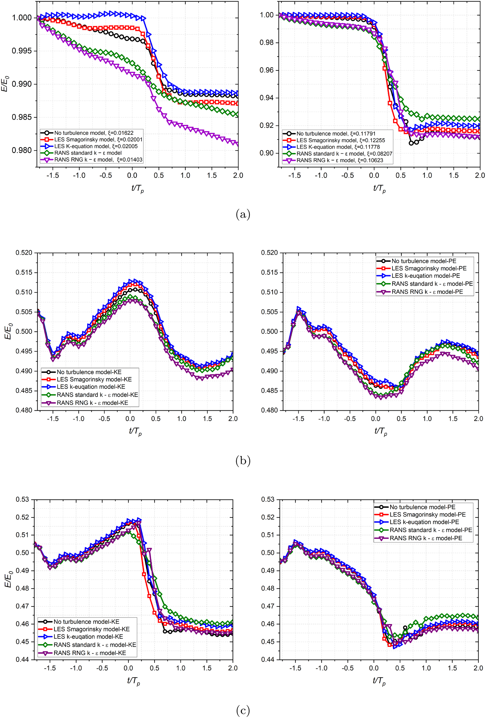
Comparison of the normalised wave energy profiles for the peak-focussed GW wave groups with or without turbulence models. (a) Normalised total wave energy profiles. (b) Normalised two wave energy components for wave groups with A = 6.8 cm (weak breaking). (c) Normalised two wave energy components for wave groups with A = 7.2 cm (strong breaking). Notation: KE is kinetic energy; PE is potential energy.
The right panel of Figure 11a presents the strong breaking cases, where the total energy profiles from all simulations decrease during the pre-breaking phase. However, the simulations using RANS turbulence models show a more rapid decline in this phase compared to the others, indicating that RANS models overestimate energy dissipation prior to breaking regardless of breaker intensity as observed in the pre-breaking energy evolution of both weak and strong breakers. Another major disparity appears in the later stage of the active breaking phase when the strong turbulence due to breaking is modelled differently by different turbulence models. The turbulence models have limited impact on the potential and kinetic wave energy for the strong breaking cases depicted in the right panel of Figure 11c. The percentages of various energy components are estimated similarly, with only minor differences observed between the cases using RANS and LES turbulence models relative to the total energy dissipation caused by breakers. Consistently with the findings in weak breaking scenarios, LES turbulence models exhibit superior energy conservation, while tests utilising RANS turbulence models dissipate energy over 1% of the total energy in the absence of breaking. As expected, the total energy dissipation due to strong breakers is considerably higher than that observed in the weak breaking cases. During the active breaking phase, the maximum energy dissipation reaches approximately 8.2% for the tests without turbulence models. It is noticeable that at the end of the active breaking phase, there is an energy gain in the water phase. The possible explanation might be that the excess energy transfers from air to water as the dominance of energy dissipation due to breaking decreases to a certain level. This results in a slight energy gain for the water phase, leading to a new equilibrium in energy distribution after the completion of the active breaking phase. However, determining the exact reason for this requires extensive analysis of the energy excess between air and water in both 2D and 3D simulations. For our objectives, it is not critical to calculate the energy dissipation rate due to breakers during the active breaking phase because the rate is assumed to be constant. In contrast to the weak breaking cases, the strong breaking case with the standard k − ϵ model can predict the occurrence of breaking and it tends to smooth and average the process of energy exchange caused by turbulence due to breaking. The other conclusions for the effects of turbulence models on the weak breaking cases still holds for the strong breaking cases. It is worth noting that the energy evolution simulated by the no turbulence model exhibits remarkably good agreement for the strong breaking case. This is likely due to the Lagrangian wave model providing accurate velocity fields prior to breaking, thereby reducing the necessity for additional turbulence corrections.
Overall, the LES k-equation turbulence model yields the most accurate numerical results for both the evolution of energy dissipation due to weak breaking and the predicted wave crests at selected locations. While the LES k-equation model exhibits a slight energy increase prior to breaking, this deviation is minimal and remains within an acceptable range. More importantly, the total energy remains nearly constant from the initial time up to breaking, aligning with predictions from our Lagrangian wave model simulations, which have been extensively validated against experimental data. As the Lagrangian wave model treats pre-breaking wave evolution as a potential flow, it ensures accurate energy conservation and velocity predictions before breaking. To preserve this key feature in our coupled model, selecting a turbulence model that minimises numerical dissipation is essential. Among the tested models, the LES k-equation approach best maintains this energy conservation trend. It also demonstrates superior performance for strong breakers compared to the other turbulence models, particularly in predicting the overall evolution of total energy. By combining the energy evolution prior to breaking onset with the crest profiles shown in Figure 10, we observe that turbulence models influence the simulations even before breaking occurs. The higher energy levels simulated by the LES turbulence models result in reproducing better wave crest profiles during propagation towards breaking onset. In contrast, excessive energy dissipation in simulations using RANS turbulence models leads to less accurate wave profiles. This finding further verifies that before wave breaking, the total energy should ideally remain nearly constant from the initial simulation time to the instant of breaking onset. Therefore, based on our present work, we consider the LES k-equation turbulence model to be the most promising for modelling breakers.
5.3 Variations on the estimation of the breaking strength parameter b
The breaking strength parameter plays an important role in connecting the kinematic and dynamic aspects of breaking waves. Its application extends to phase-averaged wave models for estimating the influence of wave spectra. The mean energy density dissipation rate per unit length of breaking crest which was originally introduced to estimate the strength parameter b by Duncan (1981, 1983) for quasi-steady breaking can be rearranged as
where ϵl is the dissipation rate per unit length and is given by E0ξ, E0 is the initial wave energy, ξ is the observed decay rate during the active breaking period, Cb is the characteristic phase speed at breaking. A few authors have provided estimates for Cb in relation to its dependence on the linear wave speed C in the wave group (Melville and Matusov, 2002; Banner and Peirson, 2007). In the present study, we adopt an estimation of Cb based on kb which represents the local wave number at the onset of breaking as proposed by Tian et al (2008, 2012). Definitions of the local wave parameters are sketched in Figure 12 as defined in Tian et al. (2012), where Hcindicates the wave crest height, and Ht1 and Ht2 denote the wave trough heights in the front and rear of the crest. Lc is the width of the crest at the mean water level, which is used to determine a local wavelength, Lb= 2Lc. Subsequently, the local wave number can be computed as kb= 2π/Lb. A local steepness which accounts for the strong asymmetries observed in breakers is defined as Sb= kb(2Hc+ Ht1 + Ht2)/4. The breaking wave speed Cb is determined by the linear dispersion relation as Cb= (g/kbtanhkbh)1/2 with a period Tb= 2π/kbCb. Figure 12 presents the variation of the breaking parameter b against the global and local wave steepness for the peak-focussed weak and strong breaking cases, considering tests with and without turbulence models. The values of ξ used to calculate the breaking parameter b are obtained by linear fits to the data during the active breaking phase, as shown in Figure 11a. As observed in Figure 13, the breaking parameter b is correlated with the energy dissipation rate. A higher energy dissipation rate results in a higher breaking parameter b. The influence of turbulence models on the simulated parameter b is fundamentally contingent on their effect on the simulated energy dissipation during wave breaking. The variation in this parameter b remains relatively limited, provided the wave breaking event is adequately simulated, as demonstrated in cases utilising LES turbulence models as well as those without turbulence models. For the peak-focussed weak breaking cases, the breaking parameter b is in the order of magnitude of 10−4, which is one order of magnitude lower than the values reported in most of the literature. Romero et al. (2012) summarised the experimental results of the breaking parameter b for early studies, where only one data point was available in the order of 10−4 for the marginal weak breaking case found in Banner and Peirson (2007). More recently, Derakhti et al. (2018) used LES simulations to reproduce 2D dispersive focussing cases for long-crest wave packets and obtained a value of b = 4 × 10⁻⁴ for their weak breaking case. However, the values of b for the peak-focussed strong breaking cases are well within the range reported in previous literature.
Figure 12
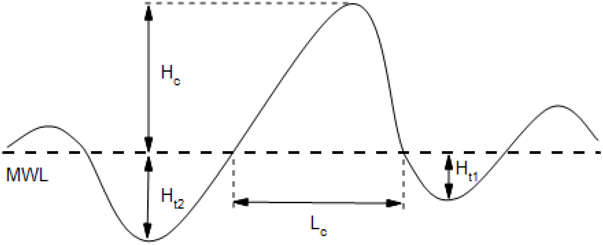
Sketch of local wave geometric parameters as defined in Tian et al. (2012).
Figure 13
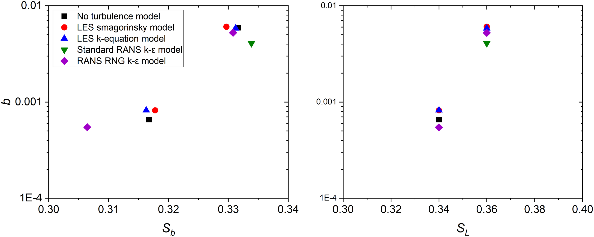
Variations on breaking parameter b for the peak-focussed GW wave groups with and without turbulence models for A = 6.8 cm (weak breaking) and A = 7.2 cm (strong breaking). Sb is the local steepness and SL is the linear global steepness for wave groups .
6 Concluding remarks
This paper underscores two significant achievements. Firstly, it presents a hybrid wave model that excels in accurately reproducing breaking events. The hybrid wave model, which couples the Lagrangian wave model with the VOF wave model within the OpenFOAM framework, has been verified and validated against experimental time histories of surface elevations, the experimental spatial wave profiles and surface profiles obtained through the Lagrangian wave model. The model consistently demonstrates its capacity to closely replicate wave conditions, as exemplified by the time histories of surface profiles at specific probes, as depicted in Figure 6. We also demonstrates the robustness and stability of the hybrid wave model when used to analyse extreme weak breaking cases which are known to be sensitive to numerical conditions in terms of the energy dissipation due to breakers, in which the total energy dissipation due to breaking during the active breaking phase is within [0.6%,1.2%] depending on the chosen turbulence model. More importantly, the method for transferring wave conditions from the Lagrangian wave model to the VOF wave model is convenient and efficient. This approach can be effectively applied to a wide range of Fully Nonlinear Potential Flow Theory (FNPT) and full Navier-Stokes (NS) Volume of Fluid (VOF) combined wave models. A similar wave tank setup to the one presented here can be used in the future to investigate the post-breaking process, including the distribution of bubble generation and droplet behaviour in three dimensions. This can facilitate a direct comparison between experimental results and numerical simulations with more realistic wave spectra related to the modelled sea state.
A central focus of this study was put on the investigation of the effects of four different turbulence models: RANS standard k −ϵ, RANS RNG k −ϵ, LES Smagorinsky Subgrid-scale (SGS), and LES k-equation SGS models for the peak-focussed weak and strong breaking cases. The performance of these turbulence models was evaluated across various aspects, including the prediction of the time at breaking onset, comparisons of wave crest profiles, the evolution of total energy due to breaking, and variations in the calculation of the breaking parameter b. LES turbulence models simulate higher kinetic energy prior to breaking while maintaining a similar level of potential energy compared to tests without turbulence models. This results in a more conservative total energy and less nonphysical energy dissipation. Consequently, breaking onset occurs slightly earlier, leading to more energetic breaking events compared to tests with no turbulence models or RANS turbulence models, ultimately resulting in a larger breaking strength parameter b. The LES turbulence models can increase total energy dissipation by up to 50% during the active breaking phase in weak breaking cases compared to the simulation without a turbulence model, as indicated by an increase from 0.8% to 1.2%. However, their impact on strong breaking cases remains limited. In contrast, the RANS RNG k − ϵ turbulence model exhibits excessive energy dissipation during wave propagation for the weak breaking case, resulting in an energy dissipation estimate during the active breaking phase that is 33% lower than that of the no turbulence model, as shown by a decrease from 0.8% to 0.6%. The standard RANS k − ϵ turbulence model fails to capture the characteristics of weak breaking due to an overestimation of turbulence prior to breaking and significantly underestimates energy dissipation in strong breaking cases. The simulation without turbulence models also produces reasonably accurate results due to the precise initial wave conditions from the Lagrangian wave model. This suggests that a well-configured numerical setup with accurate initial kinematic and dynamic data in a hybrid model can effectively predict wave-breaking behaviour that closely matches experimental measurements. More importantly, the turbulence models primarily affect the energy distribution of wave groups at the early stages before wave breaking, which in turn influences the wave breaking process, leading to variations in the associated breaking parameters. The subsequent wave evolution process is highly dependent on the early states that wave groups achieve prior to breaking. A significant observation is presented in Figure 10, indicating that the energy distribution prior to breaking onset is a critical factor influencing the evolution of the wave-breaking crest. More importantly, this work provides valuable references by systematically comparing the effects of different turbulence models on steepness-limited breaking waves with a more realistic representation of wave spectra. Overall, the coupled model with the LES k-equation turbulence model is a promising approach for accurately simulating wave breaking. It preserves energy conservation before breaking onset, similar to Fully Nonlinear Potential Flow Theory (FNPT) models, while offering affordable computational costs. Future studies can extend this framework to explore air-wave interactions within a three-dimensional numerical wave tank.
Statements
Data availability statement
The raw data supporting the conclusions of this article will be made available by the authors, without undue reservation.
Author contributions
CZ: Data curation, Formal analysis, Investigation, Methodology, Software, Validation, Visualization, Writing – original draft. EB: Conceptualization, Data curation, Investigation, Methodology, Project administration, Resources, Software, Supervision, Validation, Writing – review & editing.
Funding
The author(s) declare that no financial support was received for the research and/or publication of this article.
Conflict of interest
The authors declare that the research was conducted in the absence of any commercial or financial relationships that could be construed as a potential conflict of interest.
Publisher’s note
All claims expressed in this article are solely those of the authors and do not necessarily represent those of their affiliated organizations, or those of the publisher, the editors and the reviewers. Any product that may be evaluated in this article, or claim that may be made by its manufacturer, is not guaranteed or endorsed by the publisher.
References
1
BannerM. L.PeirsonW. L. (2007). Wave breaking onset and strength for two-dimensional deepwater wave groups. J. Fluid Mech.585, 93–115. doi: 10.1017/S0022112007006568
2
BiausserB.FrauniéP.GrilliT. S.MarcerR. (2004). Numerical analysis of the internal kinematics and dynamics of 3-d breaking waves on slopes. Int. J. Offshore Polar Engng14, 247–256.
3
BrownS. A.GreavesD. M.MagarV.ConleyD. C. (2016). Evaluation of turbulence closure models under spilling and plunging breakers in the surf zone. Coast. Eng.114, 177–193. doi: 10.1016/j.coastaleng.2016.04.002
4
BuldakovE. (2021). Wave propagation models for numerical wave tanks, in: Advanced Numerical Modelling of Wave Structure Interaction. CRC Press, 36–68. doi: 10.1201/9781351119542-2
5
BuldakovE.HigueraP.StagonasD. (2019). Numerical models for evolution of extreme wave groups. Appl. Ocean Res.89, 128–140. doi: 10.1016/j.apor.2019.05.013
6
BuldakovE.StagonasD.SimonsR. (2017). Extreme wave groups in a wave flume: Controlled generation and breaking onset. Coast. Eng.128, 75–83. doi: 10.1016/j.coastaleng.2017.08.003
7
Chasapis TassinisK. (2023). On the evolution of oceanic bubble statistics: an experimental study. Doctoral thesis (Ph.D). UCL (London, UK: Universtiy College London.)
8
ChenG.KharifC.ZaleskiS.LiJ. (1999). Two dimensional navier-stokes simulation of breaking waves. Phys. Fluids11, 121–133. doi: 10.1063/1.869907
9
ChenL. F.StagonasD.SantodH.BuldakovV. E.SimonscR. R.TaylorH. P.et al. (2019). Numerical modelling of interactions of waves and sheared currents with a surface piercing vertical cylinder. Coast. Eng.145, 65–83. doi: 10.1016/j.coastaleng.2019.01.001
10
ChristensenE. D. (2006). Large eddy simulation of spilling and plunging breakers. Coast. Eng.53, 463–458. doi: 10.1016/j.coastaleng.2005.11.001
11
ChristensenE. D.DeigaardR. (2001). Large eddy simulation of breaking waves. Coast. Eng.42, 53–86. doi: 10.1016/S0378-3839(00)00049-1
12
CraciunescuC. C.ChristouM. (2020). Wave breaking energy dissipation in long-crested focused wave groups based on jonswap spectra. Appl. Ocean Res.99, 102144. doi: 10.1016/j.apor.2020.102144
13
CuiT.HeG.JiangM.WangW.YuanL.HanD.KamathA.BihsH.. (2022). Large eddy simulation of focused breaking waves with different wave steepness. Ocean Model.179, 102122. doi: 10.1016/j.ocemod.2022.102122
14
DeikeL.MelvilleW. K.PopinetS. (2016). Air entrainment and bubble statistics in breaking waves. J. Fluid Mech.801, 91–129. doi: 10.1017/jfm.2016.372
15
DerakhtiM.BannerM. L.KirbyJ. T. (2018). Predicting the breaking strength of gravity water waves in deep and intermediate depth. J. Fluid Mech.848, R2. doi: 10.1017/jfm.2018.352
16
DerakhtiM.KirbyT. J. (2014). Bubble entrainment and liquid-bubble interaction under unsteady breaking waves. J. Fluid Mech.761, 464–506. doi: 10.1017/jfm.2014.637
17
DerakhtiM.KirbyT.BannerL.GrilliT.ThomsonJ. (2020). A unified breaking onset criterion for surface gravity water waves in arbitrary depth. J. Geophys. Res. Oceans125. doi: 10.1029/2019JC015886
18
De VitaF.VerziccoR.A.I. (2018). Breaking of modulated wave groups: kinematics and energy dissipation processes. J. Fluid Mech.855, 267–298. doi: 10.1017/jfm.2018.619
19
DevolderB.TrochP.RauwoensP. (2018). Performance of a buoyancy-modified k-epsilon and k-epsilon sst turbulence model for simulating wave breaking under regular waves using openfoam. Coast. Eng.138, 49–65. doi: 10.1016/j.coastaleng.2018.04.011
20
Di GiorgioS.PirozzoliS.IafratiA. (2022). On coherent vortical structures in wave breaking. J. Fluid Mech.947, A44. doi: 10.1017/jfm.2022.674
21
DuncanJ. H. (1981). An experimental investigation of breaking waves produced by a towed hydrofoil. Proc. R. Soc Lond. A.337, 331–348. doi: 10.1098/rspa.1981.0127
22
DuncanJ. H. (1983). The breaking and nonbreaking wave resistance of a two-dimensional hydrofoil. J. Fluid Mech.126, 507–520. doi: 10.1017/S0022112083000294
23
FuhrmanD. R.LiY. (2020). Instability of the realizable k–epsilon turbulence model beneath surface waves. Phys. Fluids32. doi: 10.1063/5.0029206
24
GiancarloA. (2009). Reynolds-averaged navier–stokes equations for turbulence modeling. Appl. Mech. Rev.62. doi: 10.1115/1.3124648
25
HigueraP.BuldakovE.StagonasD. (2021). Simulation of steep waves interacting with a cylinder by coupling cfd and lagrangian models. Int. J. Offshore Polar Eng.31, 87–94. doi: 10.17736/ijope.2021.jc821
26
HildebrandtA.SriramV.SchlurmannT. (2013). Simulation of focusing waves and local line forces due to wave impacts on a tripod structure. Proc. Int. Offshore Polar Eng. Conf., 575–581.
27
IafratiA. (2009). Numerical study of the effects of the breaking intensity on wave breaking flows. J. Fluid Mech.622, 371–411. doi: 10.1017/S0022112008005302
28
KimS. H.YamashiroM.YoshidaA. (2010). A simple two-way coupling method of bem and vof model for random wave calculations. Coast. Eng.57, 1018–1028. doi: 10.1016/j.coastaleng.2010.06.006
29
KingJ.LindS.RogersB.PK StansbyP.VacondioR. (2023). Large eddy simulations of bubbly flows and breaking waves with smoothed particle hydrodynamics. J. Fluid Mech.972, A24. doi: 10.1017/jfm.2023.649
30
LachaumeC.BiausserB.GrilliS. T.FrauniéP.GuignardS. (2003). Modeling of breaking and post-breaking waves on slopes by coupling of bem and vof methods. Proc. Int. Offshore Polar Eng. Conf., 1698–1704.
31
LarsenB. E.FuhrmanD. R. (2018). On the over-production of turbulence beneath surface waves in reynolds-averaged navier–stokes models. J. Fluid Mech.853, 419–460. doi: 10.1017/jfm.2018.577
32
LarsenB. E.FuhrmanD. R.RoenbyJ. (2018). Performance of interfoam on the simulation of progressive waves. Coast. Eng. J.61, 380–400. doi: 10.1080/21664250.2019.1609713
33
LaunderB.SpaldingD. B. (1974). The numerical computation of turbulent flows. Comput. Methods Appl. Mech. Eng.3, 269–289. doi: 10.1016/0045-7825(74)90029-2
34
LemosC. (1992). A simple numerical technique for turbulent flows with free surfaces. Int. J. Numer. Methods Fluids15, 127–146. doi: 10.1002/fld.1650150202
35
LiY.FuhrmanD. R. (2022). Computational fluid dynamics simulation of deep-water wave instabilities involving wave breaking. J. Offshore Mech. Arct. Eng.144. doi: 10.1115/1.4052277
36
LiY.LarsenB. E.FuhrmanD. R. (2022). Reynolds stress turbulence modelling of surf zone breaking waves. J. Fluid Mech.937, A7. doi: 10.1017/jfm.2022.92
37
LinP. Z.LiuP. L. F. (1998). A numerical study of breaking waves in the surf zone. J. Fluid Mech.359, 39–264. doi: 10.1017/S002211209700846X
38
LiuC.HuY. D.YangX. B.HuC. H. (2024). Numerical study of bubble rise in plunging breaking waves. Phys. Fluids36, 052111. doi: 10.1063/5.0206434
39
LubinP.GlocknerS. (2015). Numerical simulations of three-dimensional plunging breaking waves: generation and evolution of aerated vortex filaments. J. Fluid Mech.767, 364–393. doi: 10.1017/jfm.2015.62
40
LubinP.VincentS.AbadieS.CaltagironeJ. P. (2006). Three-dimensional large eddy simulation of air entrainment under plunging breaking waves. Coast. Eng.53, 631–655. doi: 10.1016/j.coastaleng.2006.01.001
41
MelvilleW. K.MatusovP. (2002). Distribution of breaking waves at the ocean surface. Nature417, 58–63. doi: 10.1038/417058a
42
NarayanaswamyM.CrespoA. C. J.Gómez-GesteiraM.DalrympleR. A. (2010). Sphysics-funwave hybrid model for coastal wave propagation. J. Hydraul. Res.48, 85–93. doi: 10.1080/00221686.2010.9641249
43
OpenFOAM (2019). User guide version 7. The OpenFOAM Foundation. (United Kingdom: The OpenFOAM Foundation)
44
RoenbyJ.BredmoseH.JasakH. (2016). A computational method for sharp interface advection. R. Soc Open Sci.3, 160405. doi: 10.1098/rsos.160405
45
RoenbyJ.BredmoseH.JasakH. (2018). Isoadvector: Geometric vof on general meshes (OpenFOAM - Selected papers of the 11th Workshop).
46
RomeroL.MelvilleW. K.KleissJ. M. (2012). Spectral energy dissipation due to surface wave breaking. J. Phys. Oceanogr.42, 1421–1441. doi: 10.1175/JPO-D-11-072.1
47
SmagorinskyJ. (1963). General circulation experiments with the primitive equations. Mon. Weather Rev.91, 99–164. doi: 10.1175/1520-0493(1963)091<0099:GCEWTP>2.3.CO;2
48
SongC.SirvienteI. A. (2004). A numerical study of breaking wave. Phys. Fluids16, 2649. doi: 10.1063/1.1738417
49
SriramV.MaQ. W.SchlurmanncT. (2014). A hybrid method for modelling two dimensional non-breaking and breaking waves. J. Comput. Phys.272, 429–454. doi: 10.1016/j.jcp.2014.04.030
50
TianZ. G.PerlinM.ChoiW. (2008). Evaluation of a deep-water wave breaking criterion. Phys. Fluids20, 066604. doi: 10.1063/1.2939396
51
TianZ.PerlinM.ChoiW. (2012). An eddy viscosity model for two-dimensional breaking waves and its validation with laboratory experiments. J. Fluid Mech.23, 036601. doi: 10.1063/1.3687508
52
WangZ.YangJ.SternF. (2016). High-fidelity simulations of bubble, droplet and spray formation in breaking waves. J. Fluid Mech.792, 307–327. doi: 10.1017/jfm.2016.87
53
YakhotV.ThangamS.GatskiT. B.OrszagS. A.SpezialeC. G. (1992). Development of turbulence models for shear flows by a double expansion technique. Phys. Fluids4, 1510–1520. doi: 10.1063/1.858424
54
YangZ.DengB. Q.ShenL. (2018). Direct numerical simulation of wind turbulence over breaking waves. J. Fluid Mech.850, 120–155. doi: 10.1017/jfm.2018.466
55
YoshizawaA. (1982). A statistically-derived subgrid model for the large-eddy simulation of turbulence. Phys. Fluids25, 1532–1539. doi: 10.1063/1.863940
56
ZouQ. P.ChenH. F. (2017). Wind and current effects on extreme wave formation and breaking. J. Phys. Oceanogr.47, 1817–1841. doi: 10.1175/JPO-D-16-0183.1
Appendix A. Formulation of Lagrangian model.
In the Lagrangian formulation for two-dimensional free-surface flows, Cartesian coordinates of a fluid particle is marked by Lagrangian labels (a,c) at the time t, which is expressed as x = (a,c,t) and z = (a,c,t). The formulation of the Lagrangian model includes the Lagrangian continuity (Equation A1), the Lagrangian form of vorticity conservation (Equation A2) and the dynamic free-surface condition (Equation A3)
where J is the Jacobian of the mapping from local coordinates to global coordinates.
where P is the pressure that is constant for a free surface and ρ is the fluid density. For inviscid incompressible fluid, functions J (a,c) and ℧(a,c) are given functions of Lagrangian coordinates, which are specified implicitly by the initial conditions. Function J (a,c) is defined by the initial positions of fluid particles associated with labels J (a,c). Function ℧(a,c) is the vorticity distribution specified by the velocity field at the initial time. Some physical and artificial surface pressure terms are added to the right-hand side of the dynamic free-surface equation to describe surface tension and simulate breaking dissipation:
The right-hand side formulation is expressed as the following
where κ is the surface curvature. In Equation A3, the first term represents the action of surface pressure that resists the motion in the direction normal to the free surface, which is controlled by the damping coefficient k (a) and is used for absorbing reflections from a boundary of a numerical wave tank opposite to a wavemaker. The second term is used to generate the surface pressure that resists changes of surface curvature, where σ (a) represents the corresponding damping coefficient. The coefficient σ introduces artificial dissipation due to the change of surface curvature κ. The effects of this term are triggered locally at the region of fast curvature changes for suppressing breaker development without affecting the rest of the wave. The action of this damping term is constrained both in time and space in order to minimise the undesirable effect of dissipation, where the action of the dissipation model is limited by the half-wavelength between the ascending and descending crossing points around a breaking wave crest. This function is activated only when the maximal acceleration of fluid particles at the crest starts to exceed a specified threshold aonand is turned off when the maximal acceleration drops below a second lower value aoff, in which the values of aon,aoff are selected according to a reasonable approximation. The last term in Equation A3 represents the action of surface pressure proportional to the surface curvature, corresponding to surface tension. γ is the ratio of the surface tension over density.
Summary
Keywords
hybrid wave model, turbulence models, Lagrangian wave model, breaking waves, deep and intermediate waters, wave groups, OpenFOAM
Citation
Zhang C and Buldakov E (2025) Evaluating RANS and LES turbulence models in hybrid wave modelling of breaking waves. Front. Mar. Sci. 12:1484783. doi: 10.3389/fmars.2025.1484783
Received
23 August 2024
Accepted
25 April 2025
Published
29 May 2025
Volume
12 - 2025
Edited by
Chunyan Li, Louisiana State University, United States
Reviewed by
Marios Christou, Imperial College London, United Kingdom
Widar Weizhi Wang, Norwegian University of Science and Technology, Norway
Updates
Copyright
© 2025 Zhang and Buldakov.
This is an open-access article distributed under the terms of the Creative Commons Attribution License (CC BY). The use, distribution or reproduction in other forums is permitted, provided the original author(s) and the copyright owner(s) are credited and that the original publication in this journal is cited, in accordance with accepted academic practice. No use, distribution or reproduction is permitted which does not comply with these terms.
*Correspondence: Chengzhao Zhang, chengzhao.zhang@ucl.ac.uk; Eugeny Buldakov, e.buldakov@ucl.ac.uk
Disclaimer
All claims expressed in this article are solely those of the authors and do not necessarily represent those of their affiliated organizations, or those of the publisher, the editors and the reviewers. Any product that may be evaluated in this article or claim that may be made by its manufacturer is not guaranteed or endorsed by the publisher.