Cetaceans and sea turtles in the northern region of the Mediterranean Cetacean Migration Corridor: abundance and multi-model habitat suitability analysis

Cardona, Luis; Amigó, Natalia; Ouled-Cheikh, Jazel; Gazo, Manel; Chicote, Carla A.

doi:10.3389/fmars.2025.1496039

ORIGINAL RESEARCH article

Front. Mar. Sci., 02 May 2025

Sec. Marine Megafauna

Volume 12 - 2025 | https://doi.org/10.3389/fmars.2025.1496039

Cetaceans and sea turtles in the northern region of the Mediterranean Cetacean Migration Corridor: abundance and multi-model habitat suitability analysis

¹Department of Evolutionary Biology, Ecology and Environmental Science and Biodiversity Research Institute (IRBio), Faculty of Biology, University of Barcelona, Barcelona, Spain
²SUBMON, Barcelona, Spain

The Mediterranean Cetacean Migration Corridor is one of the largest marine protected areas in the Mediterranean Sea. Nevertheless, little is known about the abundance and distribution of cetaceans and sea turtles in the area. A combination of aerial and boat surveys conducted in 2023 revealed the presence of seven cetaceans and two sea turtle species therein. The community was dominated numerically by two epipelagic foraging species, the striped dolphin (Stenella coeruleoalba) and the loggerhead turtle (Caretta caretta). However, based on population estimates, the majority of the community biomass was contributed by sperm whales (Physeter macrocephalus) and fin whales (Balaenoptera physalus). The population numbers of Cuvier’s beaked whales (Ziphius cavirostris) and Risso’s dolphins (Grampus griseus) were in between. When migrating fin whales were excluded from the analysis, deep divers with a high trophic position (sperm whales, Cuvier’s beaked whales and Risso’s dolphins) made a much larger contribution to the overall community biomass than epipelagic predators with a lower trophic position (striped dolphins and loggerhead turtles). Bottlenose dolphins (Tursiops truncatus), long-fined pilot whales (Globicephala melas) and leatherback turtles (Dermochelys coriacea) were observed during the surveys, but were too scarce to attempt any population estimate. Random forest models and generalized additive models identified the concentration of chlorophyll-a and the eastward current velocity as the major drivers of the distribution of epipelagic species. Conversely, the distribution of deep divers was best explained by a combination of bathymetric (standard deviation of the slope) and hydrographic (eddy kinetic energy, sea surface height and eastward or northward sea water velocity) variables. Finally, the distribution of fin whales was poorly predicted by the environmental variables considered. This evidence indicates that dynamic spatial closures might be needed to reduce the impact of fishing and maritime traffic on epipelagic predators, whereas static closures might suffice for deep divers.

1 Introduction

Overharvesting, bycatch and pollution were the main anthropogenic impacts on cetaceans and sea turtles worldwide during the second half of the 20^th century and pushed some species and populations to the brink of extinction (Wallace et al., 2011; Mittermeier and Wilson, 2014). As new regulations were enforced, the impact of such threats decreased and many populations of both groups began to recover during the first decades of the 21^st century (Duarte et al., 2020). However, the unprecedented increase of maritime traffic (Walker et al., 2019) and the development of new technologies such as offshore wind farms and deep-sea mining represent new challenges for their conservation due to the potential loss of suitable habitats (Maxwell et al., 2022).

The Mediterranean Sea supports intense human activity and has experienced a major erosion of its biodiversity (Coll et al., 2012). However, it still supports 13 breeding species of marine mammals and two nesting species of sea turtles (Notarbartolo di Sciara, 2016; Casale et al., 2018). The distribution of cetaceans and sea turtles within the basin is highly heterogeneous and the highest at-sea species diversity has been recorded in the western Mediterranean Sea (DiMatteo et al., 2022; Cañadas et al., 2023). This is because of the higher primary productivity of the western basin compared to the eastern Mediterranean Sea (Bosc et al., 2004), as food availability for air-breathing marine vertebrates is determined mostly by primary productivity. Nevertheless, the major nesting beaches of sea turtles are found in the eastern Mediterranean Sea, because of the higher sand temperature during the summer months (Casale et al., 2018).

Studies conducted during the 1990s and early 2000s identified the Balearic Sea (between the Iberian Peninsula and the Balearic Islands), as a hotspot for the conservation of cetaceans (Forcada et al., 1994, Forcada et al., 1996, Forcada et al., 2004; Raga and Pantoja, 2004; Gómez de Segura et al., 2006a and Gómez de Segura et al., 2006b). Particularly compelling was the evidence that the spring migration of fin whales, connecting their still unknown breeding grounds, somewhere in the southern part of the Mediterranean basin, and their foraging grounds in the Gulf of Lions and the Ligurian Sea, run parallel to the Iberian Peninsula’s coastline (Raga and Pantoja, 2004). As a result, the Spanish Government designated in 2018 the Mediterranean Cetacean Migration Corridor as a Marine Protected Area and proposed to the Barcelona Convention the inclusion of the area in the SPAMI List (Specially Protected Area of Mediterranean Importance). The extent of the area is 46,385.70 km² and encloses roughly the areas in between the shelf break of the Iberian Peninsula and the shelf break west to the Balearic Islands, from latitude 38° 39’ 59.379’’ to latitude 42° 18’ 57.294’’ (Figure 1). Oil extraction and mining have been forbidden within the area, but the limited information on the distribution and abundance of cetaceans and marine turtles in this Marine Protected Area has precluded the development of specific regulations on maritime traffic, although collisions have been identified as a potential threat for cetaceans in the area (Panigada et al., 2006 and Panigada et al., 2017b; Tort Castro et al., 2022).

Figure 1

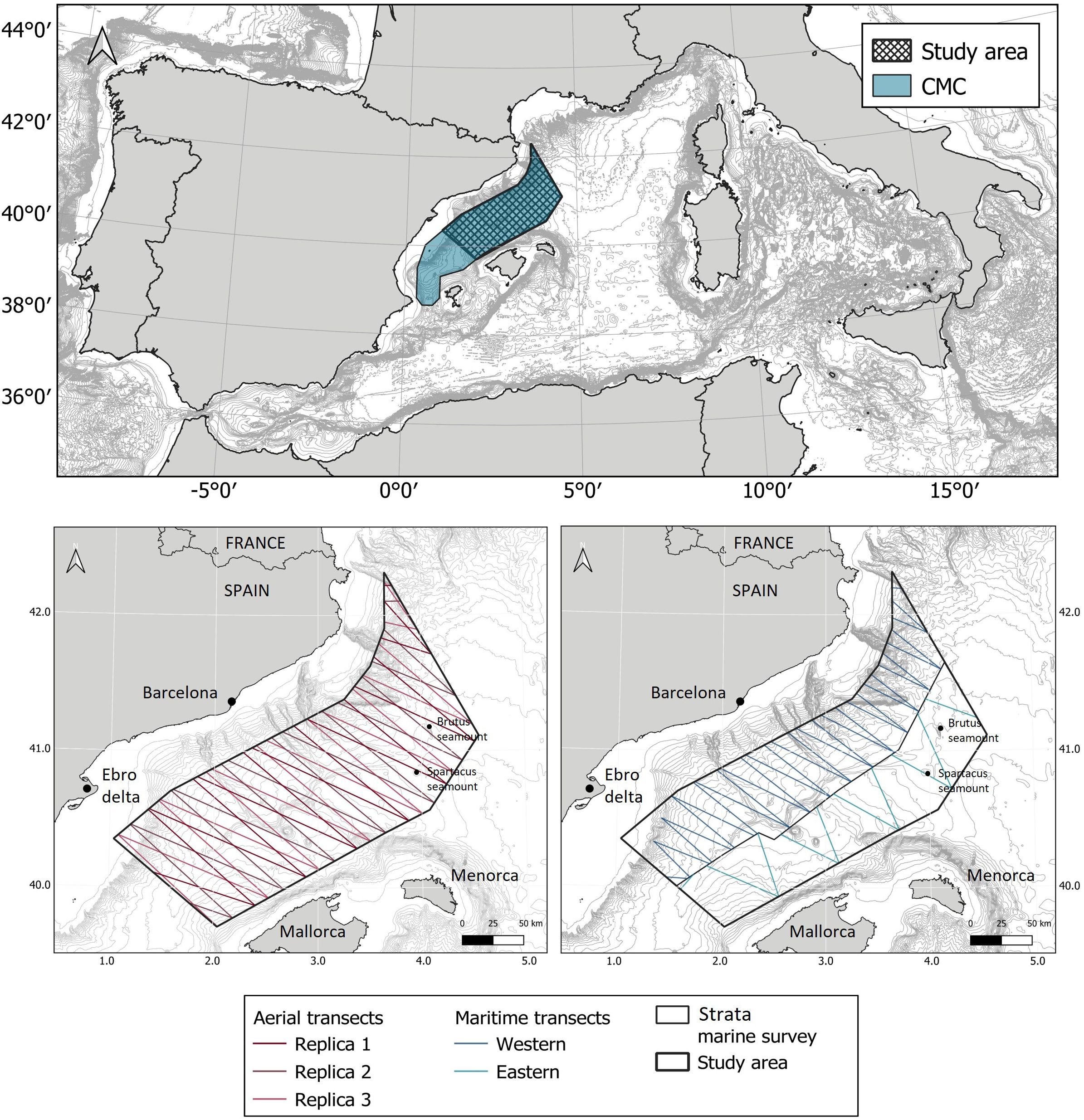
Figure 1. Study area included in the MPA of the Mediterranean Cetacean Migration Corridor (CMC) (top) and the transects designed for the aerial survey (bottom left) and boat surveys (bottom right).

Population estimates and species distribution models are critical pieces of information for the management of cetaceans and sea turtles, with aerial and boat surveys being the most common method used to gather this information. Population estimates are usually conducted within the framework of distance sampling (Buckland et al., 1993; Thomas et al, 2010), whereas species distribution models (SDMs) can be developed using different approaches. The most basic distinction is between presence-absence and presence-only models. The choice of the model depends on the type of data available, particularly whether data on survey effort was recorded alongside species sightings (Guisan and Zimmermann, 2000). Presence-absence models require both presence and absence data collected during planned surveys. Each confirmed sighting within the survey area represents a successful detection of the target species under investigation. Presence-absence models encompass a variety of statistical techniques, including Generalized Linear Models (GLMs), Generalized Additive Models (GAMs), occupancy models, or machine learning algorithms such as boosted regression trees, random forest, or support vector machines (Guisan and Zimmermann, 2000; MacKenzie et al., 2002; Brotons et al., 2004; Reisinger et al., 2021). It should be noted that combining several approaches is strongly recommended to better understand the drivers of species distribution, as modeling approaches may differ in their capacity to capture environmental gradients and the way they select the appropriate variables (Fukuda et al., 2013; Kosicki, 2020).

Random Forest is a method particularly suited to address ecological modeling problems, although it is not inherently a presence-absence model. It is a general machine learning algorithm that can be used for a variety of tasks, including classification, regression, and unsupervised learning. In the context of species distribution modeling, random forest can be used to model both presence-absence and presence-only data. Random forest models (RF) have been increasingly applied in ecological studies due to their robustness and ability to handle complex interactions among predictor variables. For cetaceans, RF have shown promise in accurately predicting species distributions and identifying important environmental variables. For example, Oppel et al. (2012) used RF to model cetacean distributions in the Mediterranean Sea, demonstrating its effectiveness in handling large and complex datasets. Similarly, Scales et al. (2017) employed RF models to predict the distribution of baleen whales in the Northeast Atlantic, highlighting the utility of machine learning approaches in marine conservation.

This study aims to improve our understanding on the abundance and distribution of cetaceans and sea turtles within the Mediterranean Cetacean Migration Corridor by developing species distribution models (SDMs) to identify areas of suitable habitat. By utilizing a combination of presence-absence models, such as GAMs and RFs, we can leverage the strengths of each approach to provide a comprehensive picture of species distribution. This information will serve as a baseline for the adaptive management of human activities in the area, ensuring the conservation of these key marine species while balancing the sustainable use of marine resources.

2 Materials and methods

The study area is located in the northern part of the Mediterranean Cetacean Migration Corridor and encompasses 32,674 km², i.e. 70% of the MPA (Figure 1).

The abundance of cetaceans and sea turtles was assessed through the combination of an aerial survey and a boat survey using Distance Sampling methodology (Thomas et al, 2010). This approach uses the perpendicular distances of individuals or groups of observed animals from the observation platform to calculate a detection function, used later to model the probability of detecting an animal given its distance from the transect line. The effective bandwidth on each side of the transect (i.e., the distance within which animals can be detected) is estimated using this detection function. Once the detection function is calculated, the estimated density can be extrapolated to the entire study area. Linear transects across the study area were designed using the software DISTANCE 7.3 (Buckland et al., 1993) in order to obtain the same likelihood of coverage within the entire area.

2.1 Aerial survey

The aerial survey included a single sampling block with three replicates (Figure 1) of the line transects (total effort Beaufort< 3 = 4,715 km; total effort Beaufort< 2 = 3,256 km) and was run from April 25th to May 5th 2023, onboard a twin-engine light aircraft with bubble windows for observation (Partenavia P68). Average flying altitude was 218.3 ± 23.4 m and average ground speed was 191.7 ± 22.2 km·h^-1. Total effort during the aerial survey was 4,715 km under Beaufort< 3 and 3,256 km under Beaufort< 2.

The team consisted of a pilot, a data recorder, and two observers. Data were recorded using the software SAMMOA (https://www.observatoire-pelagis.cnrs.fr/tools/sammoa/). During the transects, environmental and sighting data were recorded by the observers, who scanned the area through the bubble windows. Environmental data (sea state, swell height, glare, visibility and detectability) were recorded at the beginning of each transect as well as in moments of condition shifts. For all sightings, the species, position, group size and initial cue were recorded in the database. As a distance-sampling approach was used, the declination angle was recorded. This angle, relative to the horizon, is measured from the plane to the sighting when the last is abeam (directly to the side) and allows calculating the distance from the transect line to the sighting. In some cases, the sighting was detected in a position behind the abeam. In those cases, the angle was measured to the estimated position of the animal as it would have been abeam (IEO, 2022). Circle-backs were run when observers needed to confirm species identity or group size. The length of circle-backs was later removed to calculate total effort. For sea turtles, their position in the water column (on the surface vs. underwater) was also recorded, as only turtles on the surface were considered for later analysis. This is because the availability bias for this species is based on the time spent at surface according to satellite telemetry (Gómez de Segura et al., 2006a) and hence the inclusion of underwater turtles would lead to an overestimate of the total abundance.

2.2 Boat survey

The boat survey was conducted aboard a 15-meter catamaran. The survey followed a stratified design with the survey area divided into two independent blocks (Figure 2): the Western Block (17,246 km²) and the Eastern Block (14,688 km²). The Western Block was surveyed from May 24^th to June 17^th, 2023, while the Eastern Block was surveyed from September 8th to September 11th, 2023. Average boat speed during the boat survey was 6 knots (11 km h^-1) and total effort under Beaufort< 3 was 1,971 km (Western Stratum = 1,587 km; Eastern Stratum = 384 km). Data collection was conducted by a team which consisted of two observers and one data recorder. One observer scanned the 180° in front of the boat on an elevated observation crow's nest with an eye-height of 7.5 m above sea level, and the second observer scanned ahead (0º) from the deck to improve the detection probability. Environmental conditions (sea state, swell height, glare, visibility and detectability) were recorded at the beginning of the transect, every 30 minutes and each time the conditions changed. For each sighting, angle and distance from the boat to the center of each group were estimated, the latter using 7 x 50 binoculars with an internal reticule. Moreover, geographic position, time, species and group size were estimated. Group size estimation relied on visual counts, defined by three metrics: minimum number of individuals sighted simultaneously, maximum number of individuals sighted simultaneously, and the best estimate based on observer consensus. Following Whitehead (2003), a group was defined as all individuals exhibiting social interaction or coordinated behavior within five body lengths of each other. The effort, environmental and sighting data were recorded by the data recorder using Logger, the IFAW Data Logging Software (NMEA data automatically recorded every minute in a database).

Figure 2

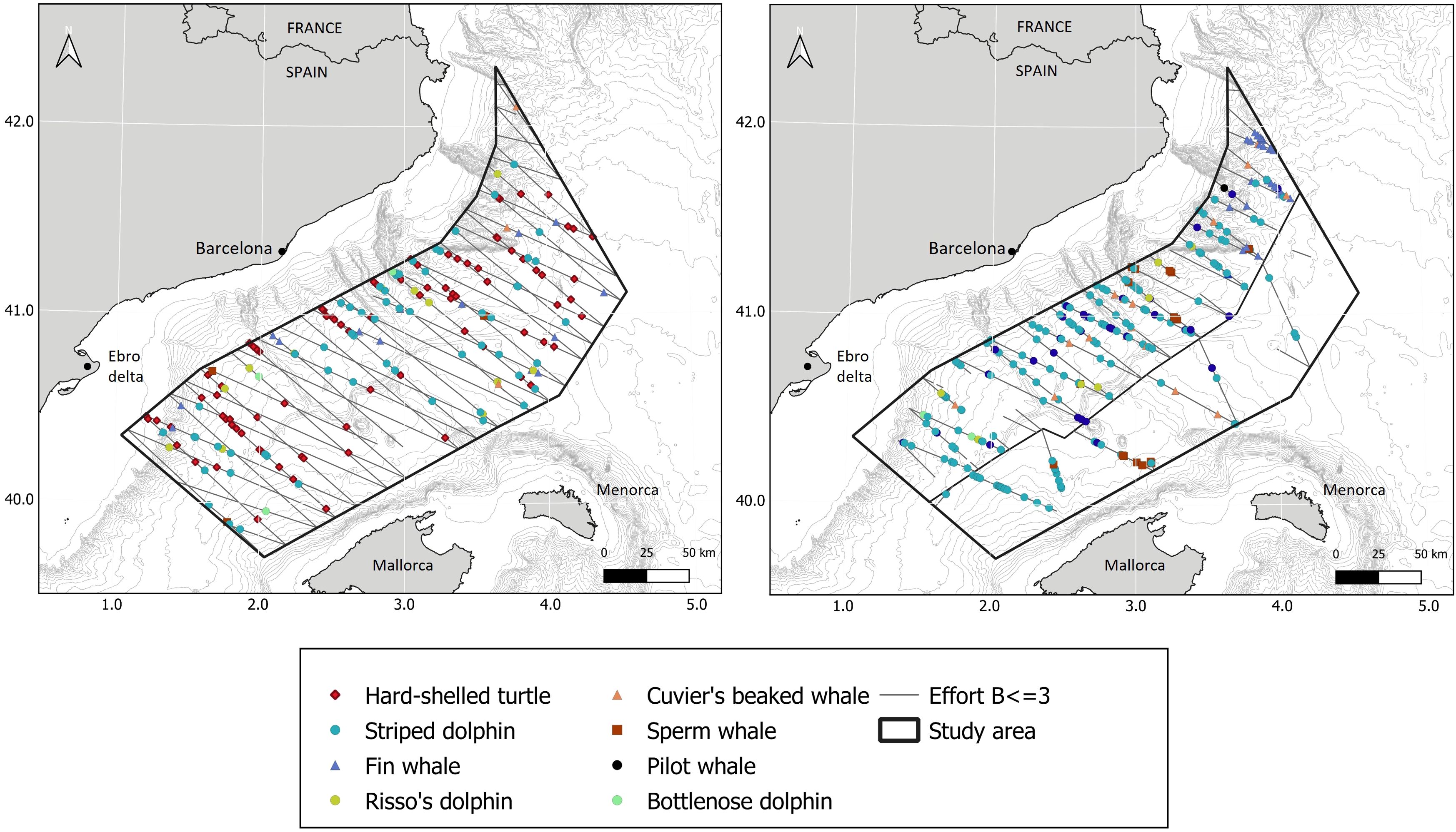
Figure 2. Sightings during the aerial (left) and boat survey (right). The line dividing the two strata for the boat survey is shown.

2.3 Population estimates

Population estimates of striped dolphins (Stenella coeruleoalba) were conducted independently for the aerial and boat surveys, as the number of sightings were high in both. Similar numbers of fin whales were spotted during the aerial and boat surveys, but the latter was conducted at the end of the spring migration of fin whales and therefore they were only spotted at the northernmost tip of the study area. In this scenario, figures resulting from the boat survey were not considered representative of the population density during the peak of the migration. Accordingly, sightings from the aerial survey were used to assess the population size of fin whales (Balaenoptera physalus), as well as the population size of Risso’s dolphins (Grampus griseus) and hard-shelled turtles. The latter category included all the sea turtles other than the leather back turtle (Dermochelys coriacea), because they are difficult to tell apart in aerial surveys. Nevertheless, the loggerhead turtle (Caretta caretta) is definitively the most abundant hard-shelled turtle species in the area and most of the sightings likely corresponded to that species. Finally, the sightings from the boat survey were used to assess the population size of Cuvier’s beaked whales (Ziphius cavirostris) and sperm whales (Physeter macrocephalus), because they were rarely spotted during the aerial survey. This is because these two species of deep divers spend most of the time underwater and hence the high speed of the aircraft reduces dramatically their detection probability. Sightings of bottlenose dolphins (Tursiops truncatus) and pilot whales (Globicephala melas) during the aerial and boat survey were too scarce to attempt any population estimate.

Data were analyzed under the framework of distances sampling (Buckland et al., 2015), using software Distance 7.5 (https://distancesampling.org). As already stated, the aerial survey included a single block with three replicates and the boat survey included two blocks with only one replicate in each (Tables 1, 2). Half-normal, hazard-rate and uniform detection functions were adjusted for each species and selected according to AIC. A single detection function for the aerial survey was adjusted for each species, due to the modest number of sightings by species and the high variability in the encounter rate across replicates. Hard-shelled turtles were the only exception, as the number of sightings in each replicate was high enough to adjust the detection function independently for each one. Likewise, detection functions were adjusted independently for each species and block of the boat survey, because each block was sampled in a different period. Cuvier’s beaked whales were the only exception, since a very low number of sightings was recorded in the eastern block for this species, so they were pooled together.

Table 1

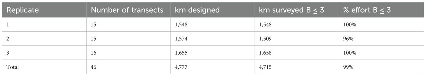
Table 1. Aerial survey total transect length per replica designed, surveyed and percentage of effort surveyed under Beaufort≤ 3 conditions.

Table 2

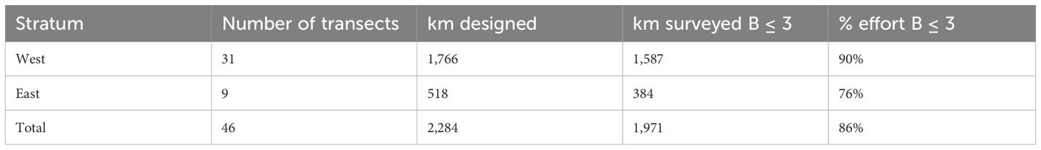
Table 2. Boat survey dates total transect length per stratum designed, surveyed and percentage of effort surveyed under Beaufort<= 3 conditions.

In all cases, models were run for each species under two different scenarios: $g (0) = 1$ and $g (0) < 1$ , being g(0) the probability of detecting an animal directly on the transect line. The first scenario ( $g (0) = 1$ ) assumed all animals on the transect line were detected, providing a minimum population estimate. The second one $(g (0) < 1)$ accounted for the availability and perception biases, providing a more realistic estimate of population size, assuming that bias correction factors are correct. The availability and perception biases used to assess $g (0)$ for each species in the second scenario are detailed in Table 3. Only effort conducted under Beaufort< 3 was considered for cetaceans and under Beaufort< 2 was considered for hard-shelled sea turtles. This is because the perception bias of hard-shelled sea turtles at Beaufort = 3 approaches 0. Estimating the striped dolphin population size using the data collected during the aerial survey was a two-step process, because of the effect of group size on the availability bias reported in the literature (Bauer et al., 2015; Gómez de Segura et al., 2006a). First, a population estimate was run independently for groups of 15 or less individuals and for groups larger than 15 individuals. Second, a global estimate was made summing the two estimates and the CI of the global population estimate was calculated as

Table 3

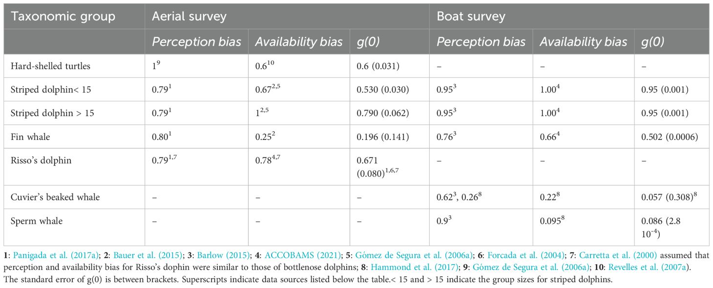
Table 3. Perception bias, availability bias and detection probability [g(0)] for each species and survey.

V A R_{g l o b a l} = V A R_{\leq 15} + V A R_{> 15} + 2 \cdot C O V \cdot (D E S_{\leq 15} \cdot D E S_{> 15})

Population numerical estimates were first reported as the mean number of individuals and the coefficient of variation (CV), expressed as %. Population numerical estimates were latter transformed into population biomass estimates using the following body mass figures: 40 kg for hard-shelled turtles, 140 kg for striped dolphins, 450 kg for Risso’s dolphins, 200–800 kg for Cuvier’s beaked whales, 30,000 kg for sperm whales and 75,000 kg for fin whales (Mittermeier and Wilson, 2014). The trophic position of each species was assessed from previously published studies using stable isotope analysis (Cardona et al., 2012; Borrell et al., 2022).

2.4 Habitat suitability models

Survey data provided information on the presence or the absence of a given species in a given place at a given time. Presence-absence habitat models allow to relate species occurrence with information on the environmental characteristics of locations (Elith et al., 2008). Here, we used Random Forest models (RF; Breiman, 2001) and Generalized Additive Models (GAM; Hastie and Tibshirani, 1986; Yee and Mitchell, 1991) to relate the presence (1) and absence (0) of species in each grid cell to the environmental variables in the same grid cell. Here, the grid resolution (4 km, approximately 0.042°) was chosen based on the resolution of the environmental products from Copernicus Marine Environment Monitoring Centre (CMEMS) platform (https://marine.copernicus.eu). Static variables were sourced or derived from ETOPO1 Global Relief Model (NOAA, https://www.ngdc.noaa.gov/mgg/global/) and dynamic environmental variables (i.e., those that change over time) were sourced from the CMEMS. Dynamic variables consisted of daily outputs from the Mediterranean Sea Physics Analysis and Forecast model and biogeochemical variables were daily outputs from Mediterranean Sea Biogeochemistry Analysis and Forecast model. See Table 4 for details on the variables and their processing. Latitude and longitude were not included as variables in the model, as we were not interested in creating descriptive models, but predictive models independent from specific geographic locations.

Table 4

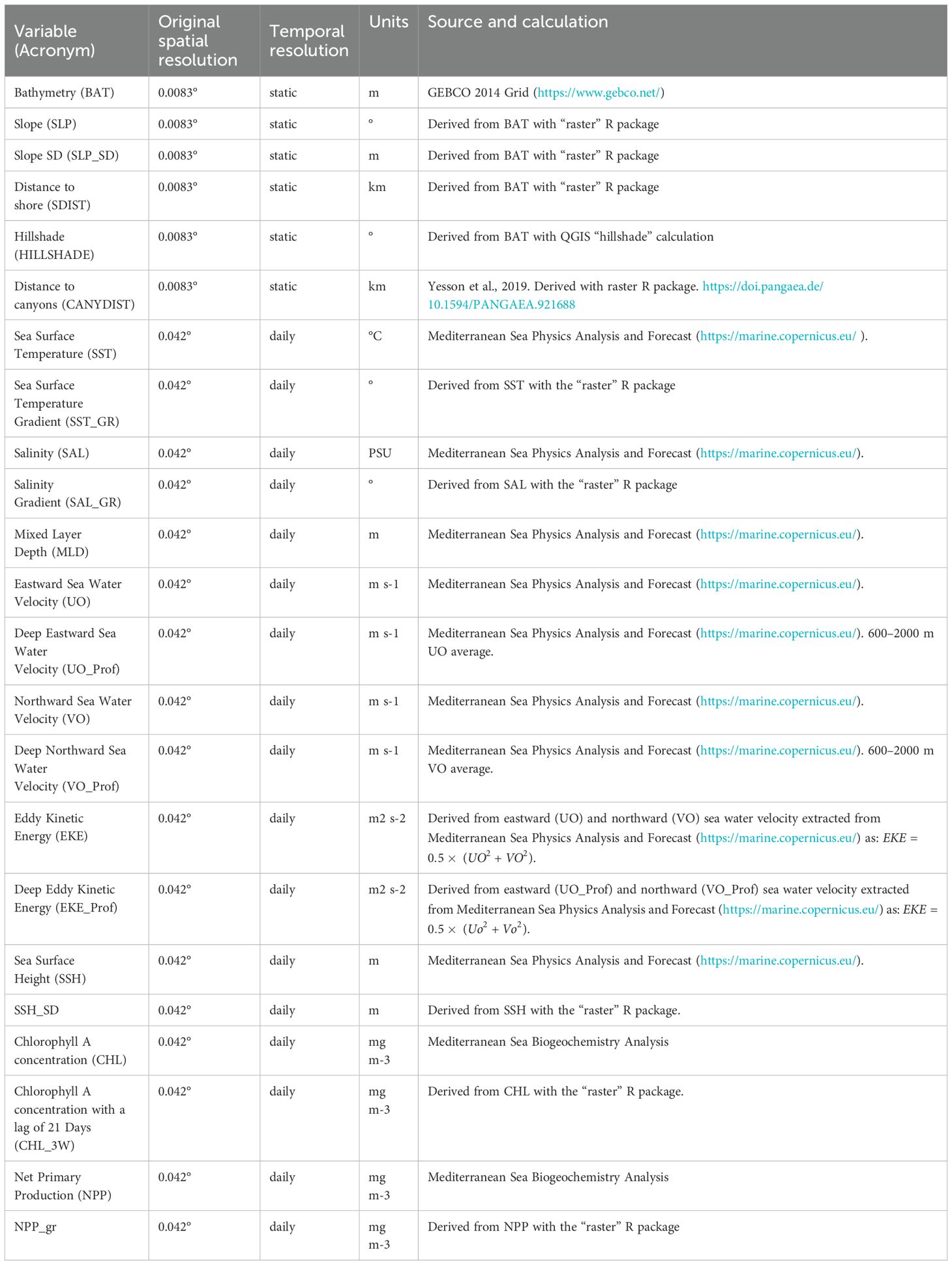
Table 4. Environmental covariates used to fit the habitat suitability models.

Species occurrences were considered as presences and all the other locations were processed as absences. This was done through the transformation of the sampled locations into a daily presence-absence grid. However, this procedure can lead to pseudo-replication (i.e., having presence and absence information in a single cell). In those cases, we kept the presence information and filtered out the absences. Moreover, we also filtered those absences that were adjacent to any presence grid cell within a temporal window of 1 day; this procedure solved the pseudo-replication issue and maximized model performance by reducing the probability that presences and absences at adjacent grid cells have similar environmental conditions on similar dates, although other temporal windows could also be useful.

The procedure described above generated an unbalanced data frame, with more absences than presences. This is not an issue for GAM but it is not ideal for the optimization of RF performance. Therefore, we conducted a stratified selection of the absences by date (by keeping 10% of absences daily; in most cases the proportion of presences to absences was 1 to 100), to ensure the representation of all the surveyed areas while obtaining a more balanced data frame. Each presence and absence location were temporally (i.e., same day) and spatially (same grid cell) matched to environmental data by averaging their values within a 4 km radius, hence accounting for uncertainty in covariate data that arises from observational error and filling in missing data.

We used a RF with a Bernoulli distribution, appropriate for presence-absence data. After filtering the data as detailed above, a second, species-specific filtering procedure was performed before fitting the final models, since we observed that only filtering out the adjacent absence cells to the presence ones did not solve entirely the possible confounding effects by cell vicinity on our models. Hence, we optimized a second buffer around the presence cells within which we filtered out absence data without compromising other presence data: 15 km for fin whale and sperm whale, 10 km for,Risso’s dolphin, hard-shelled turtle and striped dolphin, and 20 km for Cuvier’s beaked whale. Therefore, those species with more sparse data allowed for larger filtering buffers.

We identified and removed the least important environmental predictors (i.e., those not contributing to increase model performance) by using the MUVR R package (Multivariate methods with Unbiased Variable selection in R), a random forest-based variable selection algorithm that uses backward variable elimination. It uses a repeated double cross-validation accounting for repeated measures until keeping a minimal-optimal variable selection. We set the specific fit parameters required for the algorithm based on recommended guidelines to perform 50 repetitions, 8 outer sets, and retain 90% of variables per iteration (Shi et al., 2019).

To fit the RF with the filtered presence and absences and the optimized environmental predictors, we employed the caret (Kuhn, 2008) and Ranger (Wright and Ziegler, 2017) R packages. Based on the workflow outlined by Reisinger et al. (2021), we set the parameters to fit the RF with up to 1,000 trees, a minimum node size of 1, 2, 3 and 4, and tuned the number of variables randomly selected at each node (mtry of 1, 2, 3, and 4). We used the Gini index for node splitting and variable importance assessment and applied a 5-fold cross-validation method. The retained hyperparameters to fit the final model were those of the model with the highest Area Under the Receiver Operating Characteristic Curve (AUC).

We used the fitted model to generate daily spatial predictions of the habitat suitability for the entire study region for all of the study species independently. To account for model stochasticity and estimate the uncertainty associated with these predictions, we used a bootstrap approach (Elith et al., 2008; Hazen et al., 2018). We fitted the model 100 times and mapped the mean of the 100 bootstrapped daily predictions (Hindell et al., 2020; March et al., 2021). Our habitat suitability predictions range from 0 to 1, with 0 representing the least environmentally suitable locations and 1 representing the most suitable ones. To summarize our habitat suitability results, we generated prediction averages from the entire length of aerial and maritime campaigns respectively.

GAM with binomial distribution and a logit link were used. The selection of the model was based on the AIC and the explanation of the model’s deviance. In all models, the significance of the deviance was tested with a χ²-test, and a visual inspection of the residuals was made, especially to look for trends.

The general structure of the selected model was as follows:

E (p_{i}) = \frac{exp [β_{0} + \sum_{i} f_{i} (z_{i j})]}{1 + exp [β_{0} + \sum_{i} f_{i} (z_{i j})]}

where p_iwas the proportion of positive observations in grid i, β₀ was the intercept, f_i was the smooth functions of the predictor covariates, and z_ij was the value of the predictor covariate k in grid i. The models were fitted using the “mgcv” package version 1.7–26 for R version 3.0.2 (Wood and Wood, 2015), performing the manual selection.

AUC was computed for each GAM to allow for a comparison of their performance with the corresponding RF model. To do so, we used the same data structure and cross-validation procedure as applied in the RF workflow. Specifically, we performed a 5-fold stratified cross-validation using the caret R package. This approach ensures that each fold maintains the same class proportions (presence vs. absence). In each iteration, the GAM was trained on 80% of the data and evaluated on the remaining 20%. Predictions from each test fold were used to compute AUC, using the pROC R package. To ensure comparability with the final GAM structure, we used a simplified model including only the most informative variables identified in the initial GAM fitting process.

Finally, it should be noted that GAM and RF may select different environmental parameters to model the same dataset, because the first one relies on statistical significance and the second one on maximizing model performance. To assess the relevance of variable selection on the final species distribution models, we forced RF to create a species distribution model for hard-shelled turtles using two sets of the environmental descriptors selected by GAM, one including only four descriptors (SST, UO, CHL and SSH) and another one including all the statistically significant descriptors (SST, SST_GR, CHL, SLP-SD, VO, UO, and SSH). The resulting species distribution models were compared with those generated by RF using an unrestricted set of variables selected according to the procedure described previously.

3 Results

The total number of sightings during the surveys is shown in Table 5 and their distribution in Figure 2. A total of 113 sightings were recorded during the aerial survey and a total of 268 sightings during the boat survey. Hard-shelled turtles (n = 124) and striped dolphins (n = 225) were the most often spotted species during both surveys, followed by fin whales (n = 44). Risso’s dolphins (n = 19), sperm whales (n = 20), Cuvier’s beaked whales (n = 16) and bottlenose dolphins (n = 5) were also spotted during both surveys, in lower numbers. Long-finned pilot whales were spotted only once during the boat survey. Risso’s dolphins were spotted more often during the aerial survey than the boat survey; the opposite was true for sperm whales and Cuvier’s beaked whales.

Table 5

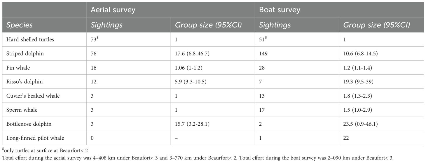
Table 5. Sightings during the aerial and boat surveys.

3.1 Abundance and habitat suitability

3.1.1 Hard-shelled turtles

The number of sightings of hard-shelled turtles was amongst the highest (Table 5) and they were the second most abundant taxonomic group, although they were ten times less abundant than striped dolphins. Total abundance, assuming $g (0) < 1$ , was 3,687 (CV = 29.1%) (Table 6).

Table 6

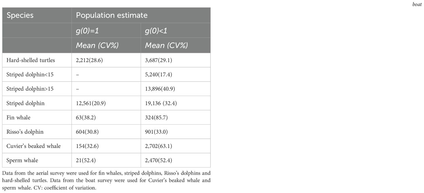
Table 6. Population estimates according to sightings.

The RF showed a high AUC value (0.80), thus indicating a high ability of this modeling approach to predict successfully the distribution of the species. The GAM developed using the same dataset was slightly lower (0.71) and explained only 14.5% of the deviance in the distribution of hard-shelled turtles. According to the information provided by both RF and GAM, the distribution of hard-shelled turtles in the study area was determined mostly by the interaction between the eastward current velocity and the concentration of chlorophyll-a, with a minor role for other parameters such as the standard deviation of slope, sea surface temperature and sea surface height (Figures 3, 4; Table 7). Both RF and GAM identified the continental slope of the Iberian Peninsula as the most suitable habitat for hard-shelled turtles, whereas the expanse of oceanic waters roughly midway between the Ebro delta and Menorca Island was the less suitable habitat (Figure 5). Nevertheless, RF and GAM disagree on the suitability of the northernmost tip of the study area. Notably, the distribution models generated by RF on the basis of the variables identified as statistically significant by GAM did not differ from those generated by GAM (Supplementary Figure 1) nor from the model generated by RF using their own selection of variables (Figure 5).

Figure 3

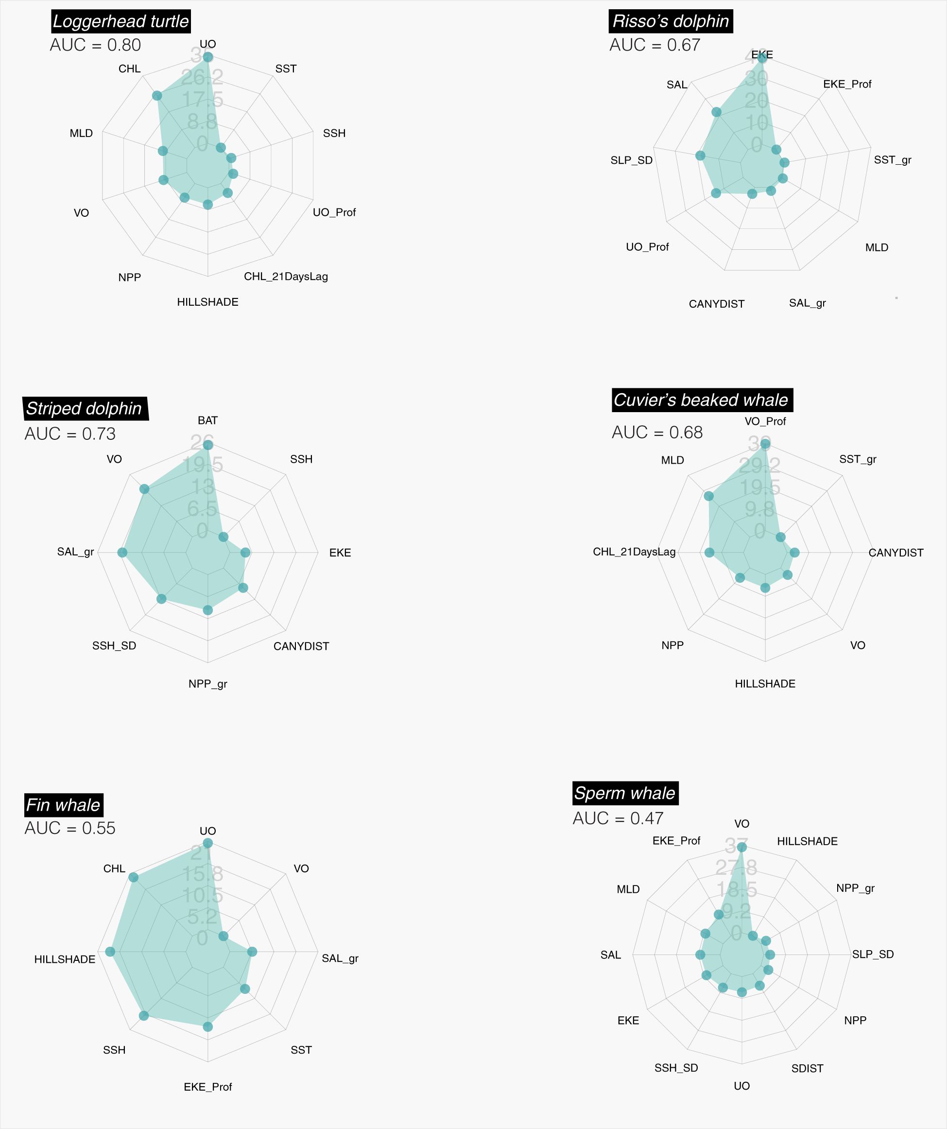
Figure 3. Relative contribution of environmental parameters to RFM. Left column: epipelagic foragers. Right column: deep divers.

Figure 4

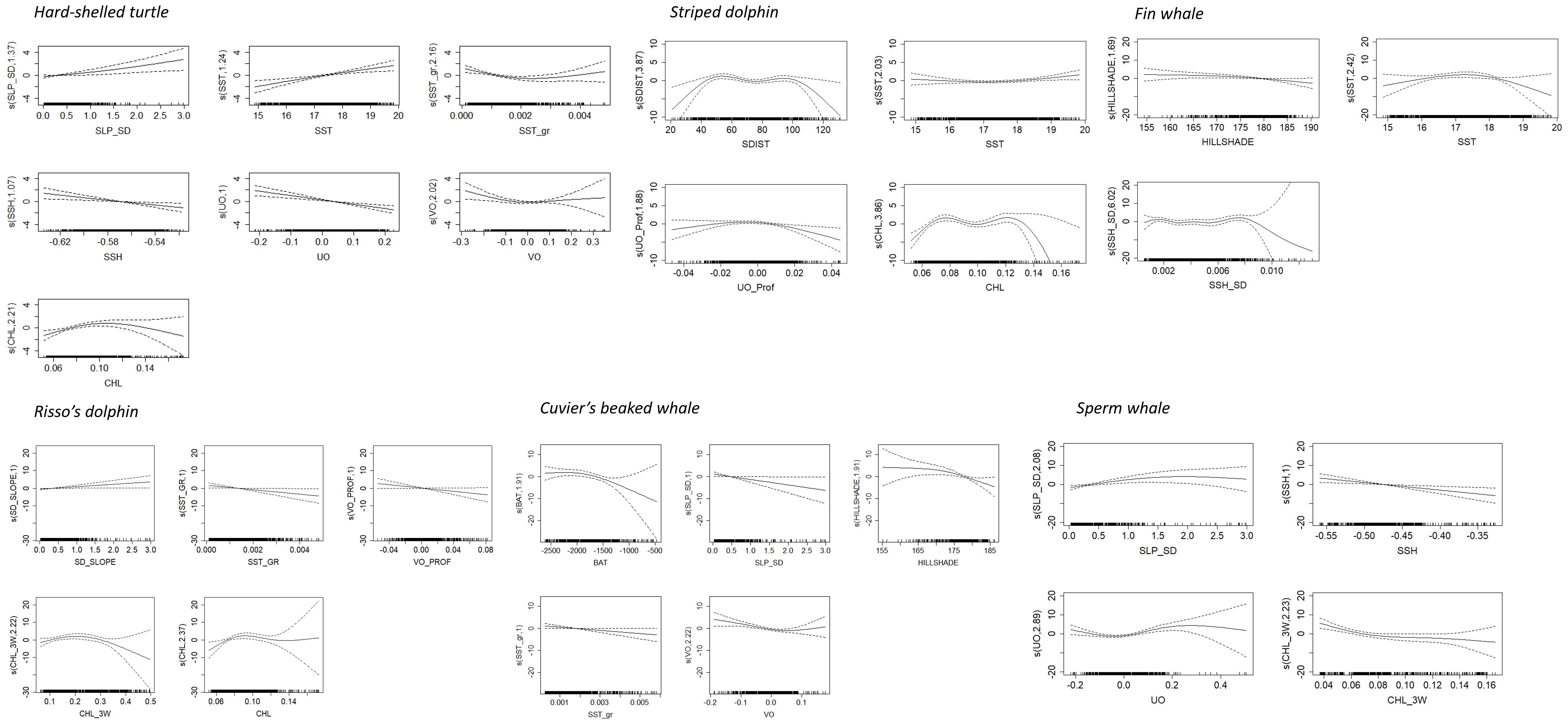
Figure 4. Predicted smooth splines of the response variable presence/absence of the six considered species as a function of the validated explanatory variables. The degrees of freedom for non-linear fits are in parentheses on the Y-axis. Tick marks above the X-axis indicate the distribution of sightings. Dotted lines represent the 95% confidence intervals of the smooth spline functions.

Table 7

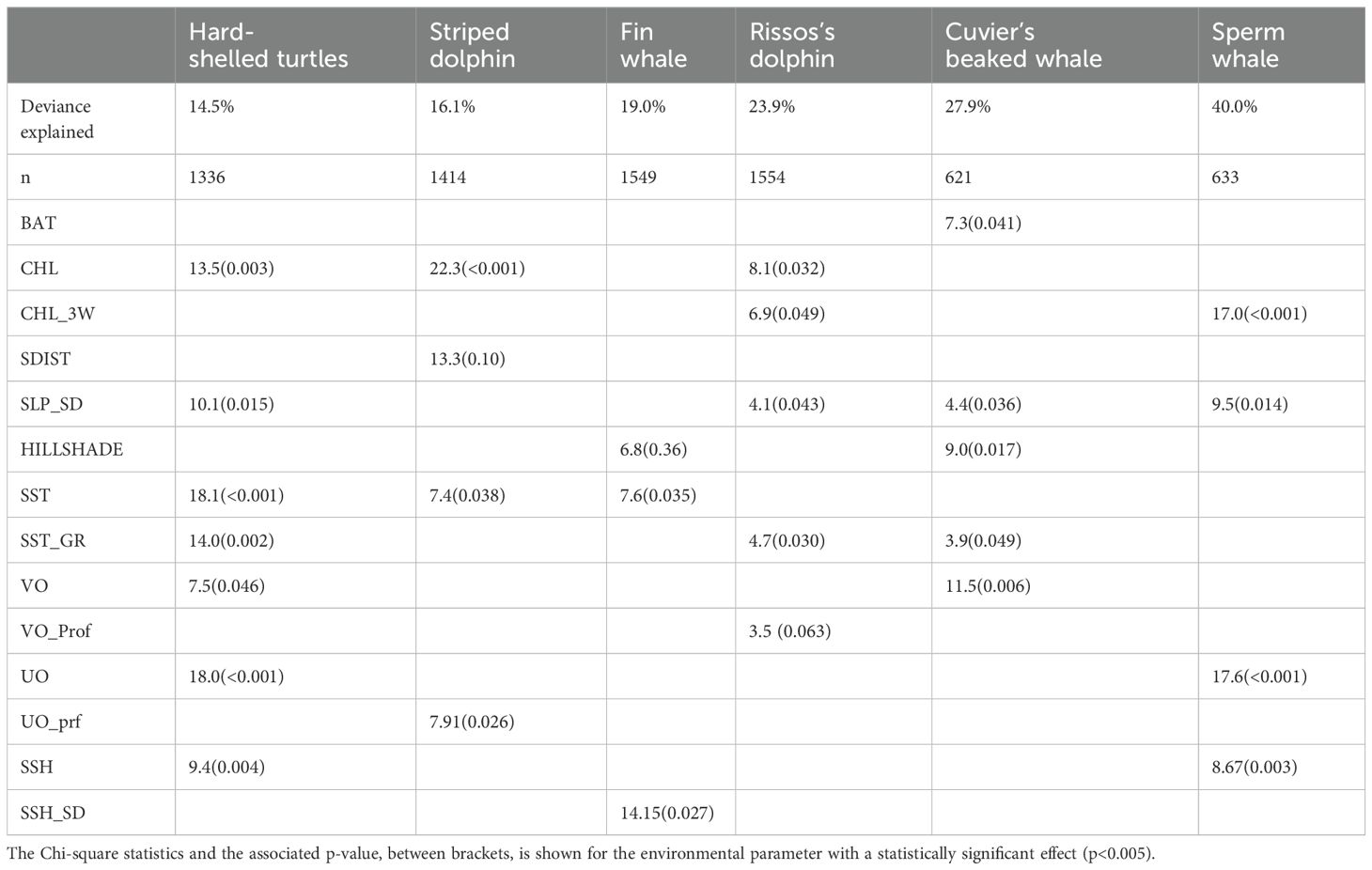
Table 7. Summary statistics of the GAMs fitted for the six studied species.

Figure 5

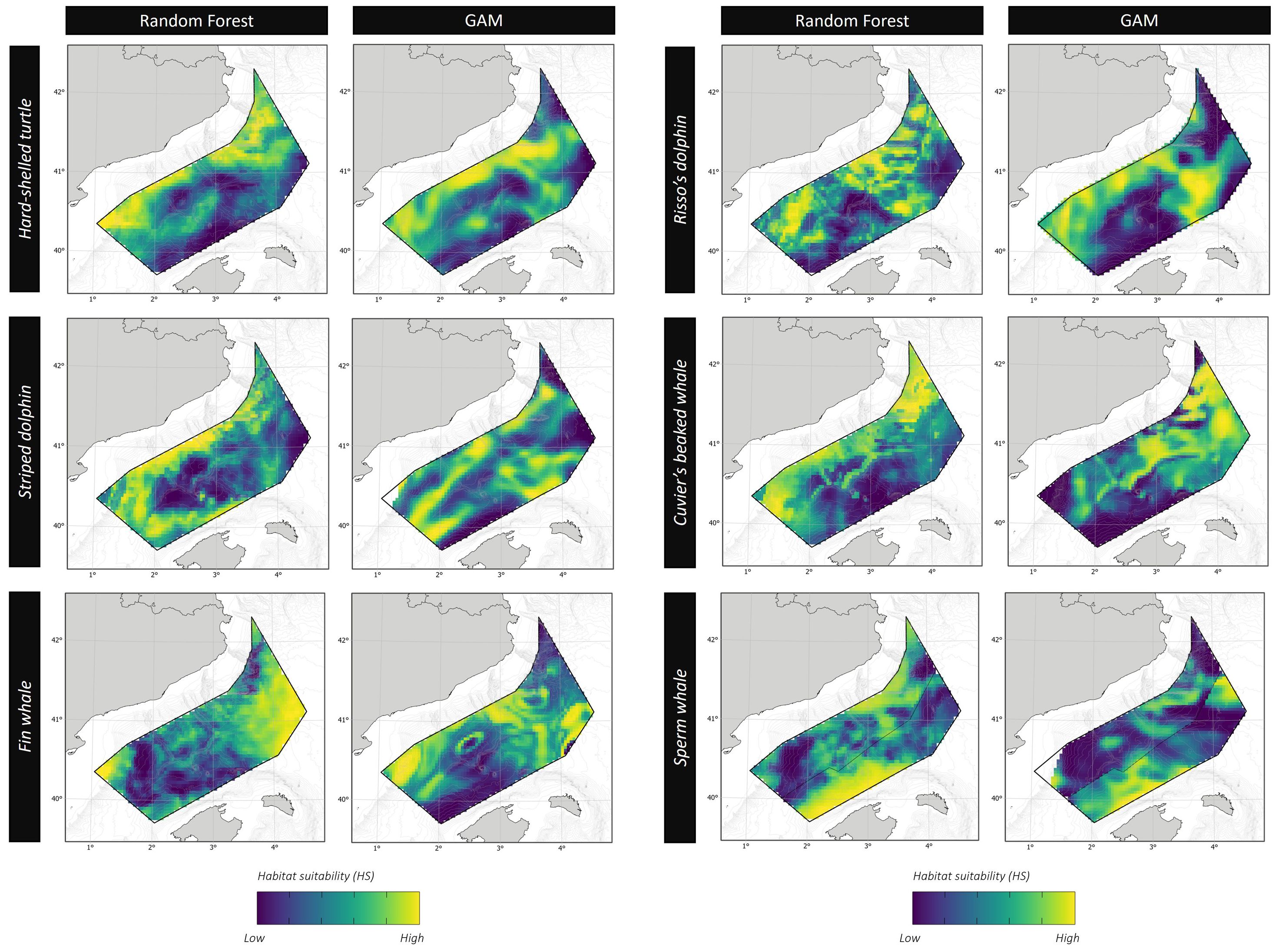
Figure 5. Habitat suitability for cetaceans and hard-shelled sea turtles within the study area. The suitability scale is relative and independent for each species. Left columns: epipelagic foragers. Right columns: deep divers.

3.1.2 Striped dolphins

The number of sightings of striped dolphins was the highest amongst all species (Table 5). Based on population estimates, striped dolphins also outnumbered any other species in the study area, both assuming $g (0) = 1$ and $g (0) < 1$ . It is worth noting that most striped dolphins occurred in pods larger than 15 individuals. Interestingly, the population estimates for the striped dolphin arising from the boat survey assuming $g (0) < 1 (m e a n_{b o a t} = 29, 537, C V_{b o a t} = 33.0 %)$ did not differ statistically from that arising from the aerial survey assuming $g (0) < 1 (m e a n_{a e r i a l} = 19, 136, C V_{a e r i a l} = 32.4 %$ ; Table 6), as the 95% CI of the difference included 0. It should be noted, however, that the confidence interval was loose in both cases. The RF model had a moderately high AUC value (0.73), with bathymetry, northward sea water velocity and salinity as the main drivers and net primary productivity and the standard deviation of sea surface height playing a secondary role (Figure 3). GAM had a similar AUC (0.76) and explained only 16.1% of the deviance in the data set, with chlorophyll-a and the distance to the shore as the main environmental drivers (Figure 4; Table 7). Nevertheless, both modeling approaches identified the regions off the continental slope of the Iberian Peninsula and the western slope of the Balearic Islands as the most suitable habitat for striped dolphins, whereas the oceanic expanse in between was identified as lowly suitable habitat (Figure 5), as for hard-shelled turtles.

3.1.3 Risso’s dolphins

The abundance of Risso’s dolphins according to the sightings during the aerial survey was 901 animals (CV = 33.0%) for the bias-corrected scenario ( $g (0) < 1;$ Table 6). RF and GAM were both moderately successful in predicting the distribution of the sightings of Risso’s dolphins (AUC = 0.67 and 0.79 respectively; explained deviance = 23.9%; Figure 3; Table 7). Both the RF and GAM revealed a preference of Risso’s dolphins for areas with a heterogeneous slope, with RF also indicating a role for eddy kinetic energy and GAM for the concentration of chlorophyll-a (Figures 3 and 4). Both approaches identified the existence of scattered patches of suitable habitat off the continental slope of the Iberian Peninsula and a distinct patch off the northwestern slope of Menorca Island (Figure 5).

3.1.4 Cuvier’s beaked whales

The estimated abundance for Cuvier’s beaked whales assuming $g (0) = 1$ was much lower than for the rest of the species, with 154 individuals (CV = 32.6%), although in the bias-corrected scenario ( $g (0) < 1)$ the abundance was even higher than that of the Risso’s dolphin resulting in 2,702 individuals (CV = 63.1%). The habitat suitability models for Cuvier’s beaked whales showed a satisfactory prediction (RF AUC = 0.68; GAM explained deviance = 27.9%; Table 7; Figure 3).

3.1.5 Sperm whales

Sperm whale estimated abundance assuming $g (0) = 1)$ was also very low (212 individuals; CV = 52.4%) and similarly to Cuvier’s beaked whale, when correcting by perception and availability biases, the abundance estimate increased to 2,470 (CV = 52.4%), although this deep diving species is difficult to estimate by visual transect. Finally, the distribution of sperm whale sightings was poorly predicted by the RF (AUC = 0.47) but the GAM performed better (AUC = 0.76) and successfully explained 40% of the deviance (Table 7). Although the RF performed poorly, it agreed with the GAM in identifying the western slope of the Balearic Islands as the most suitable habitat for sperm whales in the study area (Figure 5). The sperm whale’s GAM revealed a preference for areas with a highly variable slope and upwelling associated with cyclonic eddies, as denoted by low sea surface height (Figure 4). However, the most relevant environmental parameters were the eastward current velocity and the concentration of chlorophyll-a three weeks before the survey (Table 7), although sightings were concentrated in the less productive areas, unexpectedly (Figure 5).

3.1.6 Fin whales

Finally, the fin whale was the scarcest of the six species considered, with an abundance estimate of 63 individuals (CV = 38.3%) considering $g (0) = 1)$ and 324 (CV = 85.7%) after accounting for perception and availability biases. RF performed poorly to predict the distribution of fin whales (AUC = 0.55). Although GAM performed better (AUC = 0.76), explained only 19% of deviance (Figure 3; Table 7).

3.2 Biomass estimates

The relative contribution of each taxonomic group to the community changed dramatically when population estimates were transformed to biomass estimates (Figure 6, central panel). This was because most of the biomass in the community corresponded to sperm and fin whales, followed by Cuvier’s beaked whales and Risso’s dolphins and finally striped dolphins and hard-shelled sea turtles (Figure 6, central panel). If migratory fin whales were excluded, most of the biomass in the community was concentrated in deep divers with a high trophic position (Figure 6, right panel) and not in the numerically dominant epipelagic predators (hard-shelled turtles and striped dolphins).

Figure 6

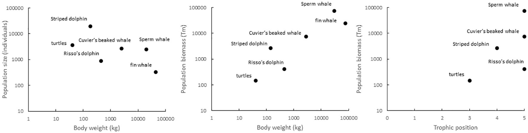
Figure 6. Relationship between population size, population biomass, body size and trophic position in the study area.

4 Discussion

The results reported here revealed that the community of air-breathing marine predators inhabiting the northern part of the Mediterranean Cetacean Migration Corridor was dominated numerically by species with a small body mass (striped dolphins and hard-shelled turtles), whereas two large-body species, the fin whale and the sperm whale, concentrated most of the biomass in the community. Nevertheless, the species considered differed largely in their habitat suitability patterns and hence the composition of the community was expected to change within the study area. Finally, the performances of RF and GAM varied largely across the studied species, without any obvious relationship with sample size and with particularly low performances of RF for fin whales and Cuvier's beaked whales. This variability probably emerged because the species differed in their responses to environmental gradients and because RF and GAM differed in the way they selected the environmental predictors to be included and their ability to capture the relevant environmental gradients at the spatial resolution considered. This is because, after accounting for collinearity, RF selected the environmental predictors that maximized the performance of the model, whereas GAM included only the environmental predictors with a statistically significant effect. As a result, RF and GAM did not always select the same environmental predictors. Furthermore, the number of sightings was small, even for the two most abundant species, which is the likely reason for the modest AUC values of both RF and GAM (Table 8) and the low values of deviance explained by GAM. Nevertheless, the performance of the resulting species distribution models were largely similar, except for fin whales and Cuvier's beaked whales, and agreed in identifying the same suitable areas for every species, except for fin whales.

Table 8

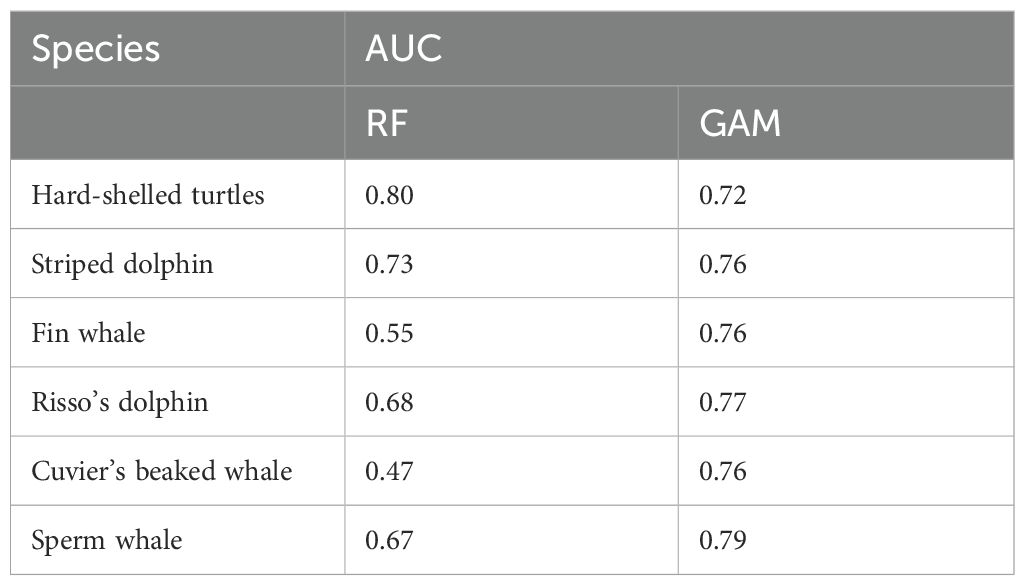
Table 8. Area under the Receiver Operating Characteristic Curve (AUC) of GAM and RF for the habitat distribution models created for the six species studied.

It should be noted that balancing the presences and absences was necessary to calculate AUC and hence enable direct numerical comparison between the performance of the RF and GAM species distribution models. This is because absences were much more abundant than presences in the original dataset and such imbalance might result into very high AUC values if the models successfully predicted absences but failed to predict presences. This is particularly relevant for the binomial GAM used in the present study, as they are based on a probabilistic framework that models the probability of the response variable (binary) using a logit link function. The performance of these models is typically assessed using metrics such as the percentage of deviance explained, which quantifies how much of the variation in the response is accounted for by the model, relative to a null model. This metric is particularly informative when the goal is to interpret the effect of individual predictors within a statistically structured model. However, this metric is unsuitable to assess the performance of RF models, as the latter are non-parametric machine learning models and no particular data distribution is assumed. Hence, AUC is the standard performance metric for this kind of classification models.

In the light of AUC, the performance of RF and GAM was rather similar, except for fin whales and Cuvier's beaked whales. Nevertheless, the final goal of using two modelling approaches was not comparing their performances, but to improve our understanding of the drivers of species distribution and make more robust estimates of habitat suitability (Fukuda et al., 2013; Kosicki, 2020). Here, by combining random forest and generalized additive models we highlighted that the habitat suitability of the species with a small body mass (hard-shelled turtles and striped dolphins) was tightly linked to parameters related to the abundance of primary producers (the concentration of chlorophyll-a or the net primary productivity), whereas that of deep divers (Risso’s dolphins, sperm whales and Cuvier’s beaked whales) was best explained by a combination of bathymetric (standard deviation of the slope, depth or hillshade) and hydrographic (eddy kinetic energy, sea surface height and eastward or northward sea water velocity) variables. Furthermore, the distribution of fin whales was poorly predicted by the environmental variables considered, likely because they were migrating along a well-defined geographic area, independently on the environmental conditions. In any case, during the spring of 2023, most of the habitats suitable for marine mammals and hard-shelled turtles within the study area concentrated along the slope of the Iberian Peninsula and the Balearic Islands, with a remarkable low habitat suitability for the oceanic expanse approximately midway the Ebro Delta and Menorca Island.

It is important noting that the spring aerial survey was the basis of most of the species distribution models presented here. This is particularly relevant for fin whales and loggerhead turtles, known to migrate seasonally (Casale et al., 2018; Panigada et al., 2017a and Panigada et al., 2024). Conversely, no seasonal migration has been described for the remaining species and hence the spring model is probably a good proxy of the year-round distribution. On the other hand, the models for Cuvier’s beaked whales and sperm whales combined data collected during the spring and late summer, for three reasons: only a few sightings were made during the aerial surveys, the spring boat cruise was restricted to the western strata due to bad weather in the eastern strata and the number of sightings during the spring boat cruise was small. Combining observations three months apart might be meaningless for migratory species, but there is no evidence that Cuvier’s beaked whales and sperm whales migrate seasonally and hence there is no reason not to increase sample size by combining observations from spring and late summer.

Previous studies reported a positive relationship between the concentration of chlorophyll-a and the population density of striped dolphins, hard-shelled turtles and fin whales at several foraging grounds in the Mediterranean Sea (Laran and Gannier, 2008; Panigada et al., 2008; Druon et al., 2012; DiMatteo et al., 2022; Tort Castro et al., 2022; Panigada et al., 2024). Hard-shelled turtles and fin whales are epipelagic predators (Panigada et al., 1999; Alvarez de Quevedo et al., 2013; Friedlaender et al., 2020) and this is also probably true for striped dolphins, in the light of the behavior of the phylogenetically close pantropical spotted dolphin (Stenella attenuata; Scott and Chivers, 2009). Oceanic loggerhead turtles rely heavily on gelatinous zooplankton (Revelles et al., 2007b; Cardona et al., 2012), whereas striped dolphins consume mostly mesopelagic fishes and squid (Aznar et al., 2017) and fin-whales primarily feed on krill (Friedlaender et al., 2020). Interestingly, most of the biomass of those forage species concentrates at the deep scattering layer during the light hours, becoming accessible to epipelagic predators only at night, when some zooplankton and mesopelagic fish species migrate to the top of the water column during their diel migrations (Quetglas et al., 2014; Lebrato et al., 2013; Olivar et al., 2022). As foraging on phytoplankton and small zooplankton is the main reason for the nocturnal migration of intermediate trophic level consumers to the top layers of the water column (Hays, 2003), it is expected that the abundance of their air-breathing predators, such as hard-shelled turtles and striped dolphins, peaks in areas rich in chlorophyll-a or high net primary productivity.

It should be noted, however, that the concentration of chlorophyll-a in the study region peaks in two distinct areas: a high concentration area over the Iberian shelf, due to the fertilization associated with the nutrients transported by freshwater runoff (Bosc et al., 2004), and a secondary peak on the off-shore region of the salinity front that usually lies over the slope of the Iberian Peninsula (Granata et al., 2004; Gordoa et al., 2008; Oguz et al., 2015). The concentration of chlorophyll-a in the latter region is enhanced by upwelling and the meandering of the North Current (Granata et al., 2004), revealed in our analyses by the module of the eastward sea water velocity. In this scenario, the probability that a pixel contains habitat suitable for hard-shelled turtles increased monotonically with the concentration of chlorophyll-a and peaked at negative values of the eastward sea velocity, denoting a strong westward current. Nevertheless, the association between the sightings of striped dolphins and the concentration of chlorophyll-a is non-monotonic, probably because distance to the shore and bathymetry are also very important for this species.

Contrarily, the results presented here do not confirm the concentration of chlorophyll-a as a major environmental driver of the distribution of fin whales at the study area, as reported previously (Panigada et al., 2017a; Tort Castro et al., 2022; Panigada et al., 2024). This is probably because the surveys were conducted during a period of extreme drought (https://www.meteo.cat/climatologia), a scenario in which primary productivity declines and the salinity front approaches the continental shelf due to weak river discharge (Sabates and Olivar, 1996; Gordoa et al., 2008). Krill distribution in the study area is poorly known, but it has been suggested to be associated with the salinity front (Ventero et al., 2019). If so, this may explain why fin whales are usually observed foraging on mid-slope, chlorophyll-rich areas during their northward spring migration across the study area (Panigada et al., 2017a; Tort Castro et al., 2022; Panigada et al., 2024). However, fin whales definitively avoid the continental shelf (Laran and Gannier, 2008; Panigada et al., 2008; Druon et al., 2012) and hence they are unlikely to find suitable foraging grounds rich in krill when the salinity front moves onshore. This hypothesis is supported by the behavior of a few satellite-tracked fin whales in the study area in the spring of 2023, as all of them were in transit across the study area and engaged in area-restricted search only when reaching the Gulf of Lions (Panigada et al., 2024).Accordingly, the concentration of chlorophyll-a is a good predictor of fin whale presence in the study area during the spring only in rainy years, when massive freshwater run-off creates a well-developed, highly productive salinity front over the continental shelf and migrating fins whales engage in foraging. In dry years, fin whales remain associated to the slope of the Iberian Peninsula during the migration, independently from foraging conditions.

The remaining three cetacean species censed in the study area are able to perform much deeper dives than those of sea turtles, striped dolphins and fin whales, reaching at least the uppermost part of the mesopelagic realm in the case of Risso’s dolphins (Arranz et al., 2019; Visser et al., 2021) and the 1000 isobath in the case of Cuvier's beaked whales and sperm whales (Tyack et al., 2006; Watwood et al., 2006). Previous research had already revealed bathymetry as the major determinant of the distribution of these three species, although primary productivity may play also a role in some areas (Gómez de Segura et al., 2006a; Praca et al., 2009; Cañadas et al., 2018; Pirotta et al., 2020; Arcangeli et al., 2023; Chicote et al., 2023). According to the data reported here, the standard deviation of the slope was a major bathymetric feature to determine the distribution of the three species.

The three deep-diving species rely heavily on mesopelagic cephalopods (Rendell and Frantzis, 2016; Santos et al., 2001; Foskolos et al., 2020; Luna et al., 2022), which engage only partially in diel vertical migrations and remain usually below the deep scattering layer and close to the seabed, even at night (Quetglas et al., 2014). In this scenario, only diving regularly over 500 m allows easy access to mesopelagic cephalopods. This lays within the diving capabilities of Cuvier’s beaked whales and sperm whales (Drouot et al., 2004; Watwood et al., 2006; Tyack et al., 2006) and may explain why they lack a clearly defined diel foraging cycle (Giorli et al., 2016). Conversely, the much smaller Risso’s dolphins forage mostly at night, when they perform shallow dives within the epipelagic realm, and it is only in the afternoon when adults engage in deep dives reaching the mesopelagic realm (Giorli et al., 2016; Arranz et al., 2019; Visser et al., 2021). This indicates that Risso’s dolphins are at least partially dependent on the diel vertical migration of their prey. In any case, the results reported here revealed a strong association to areas with a high slope standard deviation (i.e., areas with a heterogeneous slope), although it is unclear why a complex seabed bathymetry may improve access to mesopelagic cephalopods. Previous research indicated their overall scarcity within the Mediterranean Sea and their occurrence only in a few specific sites (Gómez de Segura et al., 2006a; Laran et al., 2017; Chicote et al., 2023; Cañadas et al., 2023). Submarine canyons were identified as critical habitat for the species in the study area in Chicote et al. (2023), although the study suggests a displacement to the more oceanic areas in the 2009–2021 period. Similarly, Azzellino et al. (2016) reported a distributional shift away from the coastal and continental slope habitats and related them to environmental variability, depletion of resources by fisheries and interspecies competition. The habitat suitability models developed here confirmed submarine canyons as highly suitable habitats, but also other regions with complex bathymetry, such as the Spartacus and Brutus seamounts, northwest to Menorca Island.

The capacity of sperm Cuvier's beaked whales to dive at depths greater than 500 meters and up to 1000 meters give them an almost unrestricted access to mesopelagic cephalopods, which may explain why the estimated population biomass of these two species is much larger than that of Risso’s dolphins. Suitable habitat for Cuvier’s beaked whale occurred mostly along the central and northern Iberian slope, whereas the western slope of the Balearic Islands was the area where sperm whales concentrated. Previous studies have suggested that chlorophyll-a, in combination with slope, was one of the major drivers of the distribution of sperm whales in the Mediterranean Sea (Gannier et al., 2002; Praca et al., 2009). However, the highly oligotrophic slope of the Balearic Islands (Bosc et al., 2004) supports one of the largest densities of sperm whales in the Mediterranean Sea (Pirotta et al., 2020; this study), thus suggesting that the concentration of chlorophyll-a is actually non-relevant. This hypothesis is further supported by the negative relationship between habitat suitability and the 3-week-lagged chlorophyll-a concentration, which makes little biological sense. The overall evidence is that chlorophyll-a concentration is not a driver of the distribution of sperm whales within the study area and that the observed correlations between habitat suitability and chlorophyll-a concentration may have arisen from as yet unknown interactions.

Regarding Cuvier’s beaked whales, little is known about their distribution within the Mediterranean Sea, and the available evidence about the suitability of the study area for the species is somewhat contradictory (Cañadas et al., 2018; Arcangeli et al., 2023). Nevertheless, it is worth noting that all the studies conducted to date highlight the slope off the Ebro delta and other parts of the Iberial slope as a highly suitable habitat for the species within the study area (Cañadas et al., 2018; Arcangeli et al., 2023; this study).

In conclusion, the location of suitable habitat patches for epipelagic air-breathing predators (striped dolphins, sea turtles and fin whales) within the Mediterranean Cetacean Migration Corridor is determined largely by the position of the salinity front associated with the Northern Current, whereas the distribution of suitable habitat patches for deep divers (Risso’s dolphins, Cuvier’s beaked whales and sperm whales) is mostly determined by the heterogeneity of the slope. If this hypothesis is correct, dynamic spatial closures might be needed to reduce the potential impact of fishing and maritime traffic on epipelagic predators, whereas static closures might suffice for deep divers. This is probably true also in other geographic areas, but should not be extrapolated without further assessment. On the other hand, RF and GAM yielded similar species distribution models, although sometimes selected different environmental parameters to model de distribution of the same species. This is because they are phenomenological and not mechanistic in nature and underlines the need for combining several modelling approaches to make more robust inferences about the distribution and characteristics of suitable habitats of species.

Data availability statement

The raw data supporting the conclusions of this article will be made available by the authors, without undue reservation.

Ethics statement

The manuscript presents research on animals that do not require ethical approval for their study.

Author contributions

LC: Conceptualization, Formal Analysis, Investigation, Methodology, Writing – original draft, Writing – review & editing. NA: Data curation, Formal Analysis, Investigation, Methodology, Writing – original draft, Writing – review & editing. JO-C: Formal Analysis, Writing – review & editing. MG: Investigation, Writing – review & editing. CC: Conceptualization, Data curation, Formal Analysis, Funding acquisition, Investigation, Methodology, Writing – original draft, Writing – review & editing.

Funding

The author(s) declare that financial support was received for the research and/or publication of this article. The project was supported by the Fundación Biodiversidad (Biodiversity Foundation) of the Ministry for the Ecological Transition and the Demographic Challenge (MITECO) under the Recovery, Transformation, and Resilience Plan (PRTR) funded by the European Union – NextGenerationEU.

Conflict of interest

The authors declare that the research was conducted in the absence of any commercial or financial relationships that could be construed as a potential conflict of interest.

Publisher’s note

All claims expressed in this article are solely those of the authors and do not necessarily represent those of their affiliated organizations, or those of the publisher, the editors and the reviewers. Any product that may be evaluated in this article, or claim that may be made by its manufacturer, is not guaranteed or endorsed by the publisher.

Supplementary material

The Supplementary Material for this article can be found online at: https://www.frontiersin.org/articles/10.3389/fmars.2025.1496039/full#supplementary-material

References

ACCOBAMS (2021). Estimates of abundance and distribution of cetaceans, marine mega-fauna and marine litter in the Mediterranean Sea from 2018–2019 surveys ACCOBAMS-ACCOBAMS survey initiative project. Eds. Panigada S., Boisseau O., Canadas A., Lambert C., Laran S., McLanaghan R., Moscrop A. (Monaco), 177. Available at: https://accobams.org/asi-results-for-the-mediterranean-and-black-sea-are-out/ (Accessed February 2, 2024).

Google Scholar

Alvarez de Quevedo I., Sanfélix M., Cardona L. (2013). Mortality rates in by-caught loggerhead turtle Caretta caretta in the Mediterranean Sea and implications for Atlantic populations. Marine Ecol. Prog. Ser. 489, 225–234. doi: 10.3354/meps10411