Abstract
Antarctic krill (Euphausia superba Dana) is a key species of the Southern Ocean ecosystem, immensely abundant and targeted by the krill fishery. For their sustainable management, krill distribution and biomass estimates are required, typically achieved through acoustic-trawl surveys. We explore how krill environmental DNA (eDNA) can contribute to our understanding or Antarctic krill habitat and distribution. We collected eDNA samples by filtering five liters of seawater per sample in the East Antarctic Southern Ocean from the surface (5 m depth) and seafloor (381–4422 m depth, total n = 110). We used quantitative PCR to measure Antarctic krill eDNA abundance and age, and eDNA metabarcoding to detect any krill species. This eDNA data was compared to acoustic, visual and trawl detections of Antarctic krill. Antarctic krill eDNA was common in surface samples and largely overlapped with visual and trawl detections. Highest eDNA concentrations were detected above krill swarms, with concentrations declining with increasing distance from swarms. Near recent eDNA sampling locations, krill swarms were more likely acoustically detected than near old eDNA sampling locations. Antarctic krill detections were less common in seafloor locations, and detections were concentrated in the continental slope area to the south of the survey area, both for visual detections and for recent eDNA detections. Both methods detected Antarctic krill at great depths (recent eDNA: 4300 m; visual: 3080 m). In both eDNA and trawl data, Antarctic krill was the dominant krill species, followed by Thysanoessa macrura G.O. Sars, which was particularly abundant in larval stages throughout the survey area, including at Antarctic krill swarm locations. We recommend the inclusion of eDNA data for Antarctic krill distribution estimates and understanding of habitat use, particularly in difficult-to-access areas, such as under ice or benthic habitats.
1 Introduction
Antarctic krill (Euphausia superba Dana) is a key species of the Southern Ocean, feeding on primary producers (phytoplankton) and small zooplankton, and in turn being preyed upon by a vast array of Southern Ocean predators, including fish, seabirds, seals and whales (Trathan and Hill, 2016; Schmidt and Atkinson, 2016), thus forming a central node in the Southern Ocean food web (Siegel, 2016; Everson, 2008). Antarctic krill is enormously abundant, with an estimated biomass of 379 million tons (Atkinson et al., 2009) – possibly the most abundant wild animal species on earth (Tarling and Fielding, 2016). Antarctic krill can form dense swarms near the surface (epipelagic zone; upper 250 m), which can contain hundreds, sometimes thousands of individual krill per cubic meter (Tarling et al., 2009; Cox et al., 2011). Typical smaller swarms extend 50–100 m horizontally, but occasional densely packed superswarms can extend over many kilometers in length and over 100 m in depth, containing vast amounts of krill biomass (Tarling et al., 2009; Cox et al., 2011). Antarctic krill are good swimmers and may actively move large distances (Atkinson et al., 2008; Kils, 1982; Richerson et al., 2015). They can also perform seasonal and diel vertical migration, e.g. moving to the food-rich surface (epipelagic zone) at night to avoid visual predators, and retreating to the deeper, darker mesopelagic zone during the day (Bahlburg et al., 2023; Kalinowski and Witek, 1980). They have also been observed near the seafloor in the bathypelagic zone down to 3500 m, where they may actively feed on seabed detritus year-round (Clarke and Tyler, 2008; Schmidt et al., 2011), making the benthic environment a potentially important retreat habitat for Antarctic krill. The rapid sinking of their carbon-rich fecal pellets and molts and their vertical migrations contribute to the marine biological carbon pump and long-term carbon storage in seafloor sediments (Gleiber et al., 2012; Cavan et al., 2019; Smith et al., 2025). Krill also play an important role in nutrient cycling (e.g. iron, nitrogen), which is critical for phytoplankton growth in the Southern Ocean (Schmidt et al., 2011; Cavan et al., 2019). During the Antarctic winter, sea ice forms an important part of Antarctic krill’s habitat, particularly for larval and juvenile krill (Meyer et al., 2017). Antarctic krill’s distribution range may be contracting southwards (Atkinson et al., 2019; Kawaguchi et al., 2024), likely driven by climate change pressures such as increasing water temperatures, reduced sea ice extent and ocean acidification (Flores et al., 2012; Cavanagh et al., 2021), however, the overall status of Antarctic krill population changes remain unclear (Atkinson et al., 2004; Cox et al., 2018).
Antarctic krill are also targeted by the krill fishery due to their dense nutritional and specialized pharmaceutical values, with the main fishery products sold as meal and oil (Kawaguchi and Nicol, 2020; Hill, 2013). The krill fishery is expanding, particularly around the Antarctic Peninsula, South Orkneys and South Georgia Islands and may expand into East Antarctica again after a multi-decade hiatus in this region (Kawaguchi and Nicol, 2020; Trathan, 2023). The krill fishery is sustainably managed by the Commission for the Conservation of Antarctic Marine Living Resources (CCAMLR; ccamlr.org; Constable and Nicol (2002); Miller and Agnew (2000)), which takes a precautionary approach to the management of krill fishing. To set precautionary catch limits, the CCAMLR requires biomass estimates for each management zone, which are achieved through acoustic-trawl surveys (e.g. Krafft et al., 2021; Cox et al., 2022; Hewitt et al., 2004). Acoustic-trawl surveys are typically carried out from a ship equipped with scientific (i.e. calibrated) downward looking echosounders accompanied by scientific net sampling. Both net and acoustic data are required for Antarctic krill biomass estimation (Reiss et al., 2008; Watkins et al., 2016; Cox et al., 2011). The management zones of the Antarctic Peninsula, South Orkney Islands, and South Georgia are relatively small (CCAMLR management areas 48.1, 48.2 and 48.3, see https://gis.ccamlr.org/) and accessible, and surveys are conducted regularly (Skaret et al., 2023; Fielding et al., 2014; Cutter et al., 2022). In contrast, the management zones off East Antarctica cover larger areas (CCAMLR management areas 58.4.1 and 58.4.2, see https://gis.ccamlr.org/), and distances to commercial ports are greater, making this area harder to access and more difficult to survey comprehensively. As a result, East Antarctic management zones are less frequently surveyed, leading to sparser temporal and geographic coverage of distribution and biomass surveys in this region (Jarvis et al., 2010; Cox et al., 2022; Baldo et al., 2006), which makes accurate and up-to-date Antarctic krill biomass estimates in East Antarctica challenging.
Here we explore whether environmental DNA (eDNA) – genetic material shed into the environment by all organisms, including krill – can provide an additional data layer to determine Antarctic krill distribution and abundance. The use of eDNA-based surveys is rapidly expanding across a huge range of habitats, including marine, freshwater and terrestrial (Ruppert et al., 2019; Taberlet et al., 2018). In the marine environment eDNA surveys are for example used to determine reef biodiversity (Dugal et al., 2023; Mathon et al., 2022), to assess species distributions (Yu et al., 2022; Gargan et al., 2017) or to detect marine invasive species (LeBlanc et al., 2020; Ellis et al., 2022), to name a few applications.
Typically, two methods can be employed when assessing eDNA samples for species presence and/or abundance: firstly, species-specific assays using quantitative PCR (qPCR) can be used to assess the presence and abundance of eDNA shed by a single species (Langlois et al., 2021). These markers need to be carefully designed and validated to ensure their species-specificity, as cross-amplification of eDNA of different species could lead to false positive detections (De Brauwer et al., 2023; Langlois et al., 2021). Species-specific assays are typically more sensitive at detecting the presence of a species than metabarcoding assays (see below; Yu et al., 2022; McColl-Gausden et al., 2023) and separate assays have been developed to detect the presence and distribution of many species, including marine invasive species (Clarke et al., 2023; Roux et al., 2020; Wood et al., 2017). eDNA abundance can correlate with species abundance (Rourke et al., 2022; Lacoursière-Roussel et al., 2016; Yates et al., 2019; Salter et al., 2019), but calibrations are difficult and many variables (e.g. volume of the body of water, currents, eDNA degradation properties) can affect eDNA abundance, persistence and detectability (Yates et al., 2021). As eDNA may persist in some environments for extended periods, several studies have attempted to determine eDNA fragmentation by developing sets of species-specific markers of different amplicon length (Jo et al., 2017; Bylemans et al., 2018; Suter et al., 2023). More fragmented eDNA could indicate longer time since eDNA shedding, and incorporating such temporal aspects to eDNA-based surveys could greatly aid the interpretation of eDNA abundance measurements.
Secondly, metabarcoding markers can be used to detect multiple taxa simultaneously, for example all animal species (Suter et al., 2021; Nester et al., 2024; Jeunen et al., 2019) or all fish species (Miya, 2022; Bessey et al., 2020). Metabarcoding markers amplify sections of genes or DNA that are shared between all targeted taxa and act as ‘barcodes’: these DNA sequences differ between taxa, and through comparisons to reference databases the taxonomic composition of mixed eDNA samples can be determined (Deiner et al., 2017). Metabarcoding data can provide presence/absence information of taxa, as well as an estimate of relative abundance of taxa within a sample. Through elaborate calibrations taxa abundance across samples can be estimated from metabarcoding data, but these methods are complex, and not typically employed (Deiner et al., 2017; Luo et al., 2022).
In this study, we assess how eDNA-based methods can contribute to Antarctic krill surveys, using eDNA samples collected in East Antarctica from seawater collected near the surface and the seafloor. We firstly use two Antarctic krill-specific qPCR markers of different lengths (Suter et al., 2023) to assess Antarctic krill eDNA abundance and eDNA age. We use the eDNA concentration of the short marker to estimate overall krill eDNA abundance. In addition, we estimate the age of Antarctic krill eDNA in each sample by comparing the relative abundance of the short and the long marker using a model fitted to experimental data of known age and the concept that if the short and long markers are similarly abundant, the eDNA is considered relatively intact and therefore recent. If the short marker is more abundant than the long marker, the eDNA is considered fragmented and therefore old. Secondly, we use a euphausiid-specific metabarcoding marker that can detect any Southern Ocean krill species (Suter et al., 2023), revealing overall krill distribution patterns in the Southern Ocean. To achieve a broad, semi-quantitative eDNA abundance estimate of all krill species, we use the species-specific assay to calibrate the metabarcoding data across samples.
We then compare this eDNA-data to other Antarctic krill survey methods, including acoustic, visual and trawl surveys, to get a holistic perspective on Antarctic krill distribution and abundance in the Southern Ocean. We explore how Antarctic krill eDNA spreads and decays through the Southern Ocean environment, assess whether krill eDNA abundance and age patterns are reflected in Antarctic krill assessments of other data streams and highlight strengths and challenges for each data stream. Lastly, we recommend how eDNA-methods should be used in conjunction with other data streams in future surveys to improve our understanding of Antarctic krill distribution and habitat use.
2 Methods
2.1 Survey area
Multidisciplinary data was collected on board the RV Investigator on a research expedition named “Trends in Euphausiids off Mawson, Predators and Oceanography (TEMPO)” (IN2021_V01) between 13 February and 12 March 2021 in the eastern sector of the CCAMLR Division 58.4.2. The survey area was divided into six longitudinal transects (transect 1: 55°E; transect 2: 60°E; transect 3: 65°E; transect 4: 70°E; transect 5: 75°E, transect 6: 80°E), south of 62°S for transects 1 – 4, and south of 63°S for transects 5 and 6, with the southern end of each transect limited by the sea ice edge, varying between approximately 65°S and 68°S (Figure 1). Multiple data streams were collected: eDNA, acoustic, visual and trawl data (Table 1). The research was conducted under the Antarctic Marine Living Resources Conservation Act 1981 (Australia) Permit AMLR 20-23-4512.
Figure 1
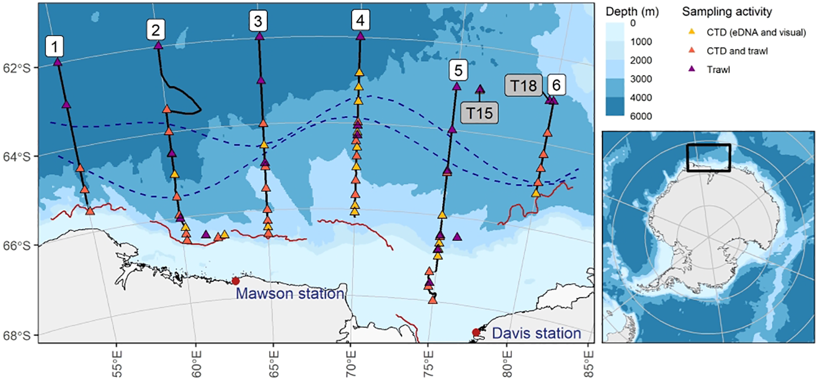
Overview of the survey area in relation to the broader Antarctic (map inset) and collected samples. Numbers 1 – 6 (white background) denote the six survey transects. Triangles denote sampling stations; black lines represent acoustic data collection along transects (1-6). T15 and T18 (grey background) indicate the location of two targeted krill swarms. Dotted lines indicate Southern Ocean oceanic fronts during the TEMPO voyage following Foppert et al. (2024): the northern line denotes the Southern Antarctic Circumpolar Current Front, at southern line the Southern Boundary of the Antarctic Circumpolar Current. The red wavy lines south of each transect indicate the sea ice edge at the time of each transect.
Table 1
| eDNA qPCR | eDNA metabarcoding | Acoustic | Visual | Trawl – RMT8 | Trawl – RMT1 | |
|---|---|---|---|---|---|---|
| Target species | E. superba | Any euphausiid species | E. superba | E. superba | Any euphausiid species | E. superba, T. macrura, ‘other’ euphausiid (grouped) |
| Target developmental stage | Any, plus faeces, moults, etc | Any, plus faeces, moults, etc | Adult, juvenile | Adult, juvenile | Adult, juvenile | Larvae |
| Data type | Krill eDNA presence, abundance and age | Krill eDNA presence, estimate of eDNA abundance | Krill biomass, krill density | Krill abundance | Krill density | Krill density |
| Detection unit | DNA fragments | DNA fragment | Acoustic reflection of swarms | Video footage | Trawl catch | Trawl catch |
| Radius of detection | Unclear; potentially ~2.8 km for recent, further for old eDNA | Unclear – likely multiple km | 250 m from ship | ~5 m from camera | ~200 m depth | ~200 m depth |
| Sampling depth | Surface (5 m), Seafloor (down to 4422 m) | Surface (5 m), Seafloor (down to 4422 m) | Surface (within 250 m) | Surface (5 m), Seafloor (down to 4422 m) | Surface (within 200 m) | Surface (within 200 m) |
| Sampling location | At CTD stations (n = 50) | At CTD stations (n = 50) | Continuously | At CTD stations (n = 50) | At trawl stations (n = 53) | At trawl stations (n = 48) |
| Detection time | Potentially hours (short) for recent DNAPotentially days (long) for old DNA | Potentially days | Immediate | Immediate | Immediate | Immediate |
| Strengths | - Large temporal, geographic and depth coverage - eDNA abundance and age provide dynamic picture - Any developmental stage detectable |
- Large temporal, geographic and depth coverage - Any Krill species can be detected - Any developmental stage detectable |
- Precise estimate of biomass - Continuous survey - Fast data processing |
- Any depth can be surveyed - Estimate of krill abundance - Fast data processing |
- Developmental stage, sex, size of krill measurable - Any Krill species can be detected - Fast data processing |
- Larval stages can be differentiated - Multiple krill species can be detected |
| Challenges | - Data processing, analysis and interpretation complex and slow - Origin of eDNA variable - Developmental stage, size etc not measurable - Relatively sparse data collection |
- Data curation complex and slow - Abundance estimates imprecise - Origin of eDNA variable - developmental stage, size etc not measurable - Relatively sparse data collection |
- Only adult/juvenile krill detectable - limited detection radius - only immediate presence of krill detectable |
- Very limited detection radius - Only immediate presence of krill detectable - Only adult/juvenile krill detectable - Species ID uncertain - Relatively sparse data collection |
- Limited depth - Only adult/juvenile krill detectable - Relatively sparse data collection - Krill swarms are often missed |
- Adult/juvenile krill not representative - Limited depth - Relatively sparse data collection - Larvae of several krill species cannot be differentiated - Slow data processing |
Data streams collected in this study: what, where and how they measure presence or abundance of krill species, and a summary of their strengths and challenges.
2.2 Data collection
2.2.1 eDNA samples
2.2.1.1 Sample collection
Seawater samples (5 L each) were collected at 50 CTD stations. At each station, a sample was collected from the surface (approximately 5 m depth) as well as from near the seafloor (seafloor depth at CTD stations ranged from 381 m to 4422 m depth), resulting in a total of 98 CTD samples (two seafloor eDNA samples were unsuccessful). CTD operations were conducted using Sea-Bird SBE911 instrumentation and 31 x 12 L Niskin bottles on a rosette. In addition, two eDNA samples each were collected within two krill swarms (T15 and T18) from the ship’s uncontaminated seawater line (5 L, depth approximately 5 m), and as the ship was moving away from the krill swarm, four further samples were collected at each krill swarm (n = 12). Seawater was transferred from the CTDs into a 5 L Cole-Parmer essentials wide mouth carboy (Cole-Palmer), or directly collected in these carboys if sampled from the uncontaminated seawater line. Samples were kept in a refrigerator at 4°C until filtering. Samples were filtered onto hydrophilic polyvinylidene fluoride membrane filter discs (5 μm pore size, 47 mm diameter; Merck) using a Masterflex L/S peristaltic pump (John Morris Scientific), either until all water was filtered (most samples), or until the filter got clogged, in which case the filtered volume was recorded. Every 10th sample was a field control consisting of 5 L Milli-Q water processed as described above. After each filtering round, all filtering equipment and laboratory desk surfaces were sterilized using 1% bleach followed by thorough rinsing with Milli-Q water. After filtering, every filter was halved, and both halves stored in separate 1.5 mL DNA LoBind Tubes (Eppendorf), which were stored at -80°C until DNA extraction.
2.2.1.2 DNA extraction
DNA was extracted from one half filter per sample, while the other half was kept for biobanking (Jarman et al., 2018) at -80°C for future studies. Samples were sent to eDNA frontiers (eDNA frontiers, Perth, Australia; http://www.ednafrontiers.com/) for DNA extraction using Qiagen DNeasy Blood & Tissue Kit (Qiagen) with the following minor modifications from the manufacturer’s protocol: 540 μl of buffer ATL and 60 μl proteinase K were added to the filters and incubated at 56°C overnight, and samples were eluted in 100 μl elution buffer. Nine extraction blanks containing no filter material were extracted with the samples.
2.2.2 Species-specific E. superba assay
2.2.2.1 qPCR markers and conditions
To estimate Antarctic krill eDNA concentrations and eDNA age, two species-specific primer combinations developed by Suter et al. (2023) were used to amplify a short 16S rRNA gene fragment (henceforth called “short marker”) and a long 16S rRNA gene fragment (henceforth called “long marker”). The short and long marker use the same forward primer (E_superba_16S_F3: 5’-TATTAAAGGATCATTCACACA-3’) and fluorescent probe (E_superba_16S_Probe: 5’-/56-FAM/CGCCCCAAT/ZEN/AAAATAAATTCCACAAT/3IABkFQ/-3’), but different reverse primers, resulting in different lengths of amplicons: the short marker uses the E_superba_16S_R1 reverse primer (5’-AAGTGGAGTAGTTGATTAAAAC-3’), resulting in an amplicon length of 126 base pairs (bp), while the long marker uses the E_superba_16S_R3 reverse primer (5’-GTGCTAAGTAACTCGGCAAA-3’), resulting in an amplicon length of 412 bp. Quantitative PCR (qPCR) amplifications were conducted in 10 μL total reaction volume, including 2X PrimeTime gene expression master mix (integrated DNA Technologies), 0.5 μM of forward and reverse primer, 0.25 μM Probe and 2 μL of undiluted DNA template.
All qPCR amplifications were done in triplicates on a QuantStudio 6 Real Time PCR System (Thermo Fisher Scientific) using 384 well plates with the following cycling conditions: 95°C for 3 min, 45 cycles of 95°C for 15 sec, 60°C for 30 sec, 65°C for 45 sec, followed by a final extension of 72°C for 2 min. All qPCR plates included triplicates of non-template negative controls (NTCs) and positive control (gblock fragment with 100 copies, see Suter et al. (2023)). Pre-PCR setups were prepared in a physically separate and PCR product free laboratory to minimize the risk of contamination.
2.2.2.2 Limits of detection and quantification
The copy number of gblock fragments per μL was calculated from the DNA concentration – measured using a Qubit DNA HS assay kit with a Qubit 2.0 Fluorometer (Life Technologies, Carlsbad, CA, USA) – and the molecular weight of the gblock fragment. To determine both the limit of detection (LOD) and limit of quantification (LOQ) for each marker, the gblock fragment was serially diluted to the following copy numbers per dilution standard: 100, 10, 2, 1, 0.5, 0.25, 0.125, 0.0625. qPCR amplifications were done in 12 replica per marker per standard with the PCR conditions as described above. The lowest standard with 95% of amplifications across all replicates determined the LOD, and the lowest standard with a coefficient of variation (CV) below 35% determined the LOQ (Klymus et al., 2020b). To derive the LODs, LOQs and primer efficiencies of the assay, the data was analyzed in RStudio (v 2022.02.2) following Klymus et al. (2020a) and Suter et al. (2023).
2.2.2.3 eDNA abundance calculations
qPCR results were quantified if at least two out of three technical replicas were within an acceptable quantification cycle (Cq) range, following Suter et al. (2023) and De Ronde et al. (2017). Acceptable ranges increased with increasing mean Cq value (range for mean Cq < 32 was 0.5, for > 32 it was 0.7, for > 33 it was 0.9, for Cq > 34 it was 1.3 and for > 35 it was 1.5). Outliers falling outside of these ranges were excluded if the other two technical replica fell within the acceptable range. Average Cq values of acceptable technical replicas were used. qPCR results that only had Cq values for one of three technical replicas were excluded. Copy number per qPCR sample were calculated separately for each qPCR plate using the intercept and slope calculated for each marker during the standard curve assessment, the Cq value of the samples and the Cq value of the standard gblock fragments (100 copies) on each qPCR plate. If copies detected in both markers per sample were below the limit of detection for three technical replicas, the data was removed. If only one of the two markers was below this threshold, copy numbers were retained, as the sample was considered to contain krill eDNA. The copy numbers per PCR amplification were then multiplied by 100 to calculate copy numbers per 5 L sample (DNA of half a filter eluted in 100 μl, 2 μl used per qPCR), and in samples were less than 5 L of seawater was filtered due to filter clogging, the copy number was divided by the proportion of 5 L that was filtered for those samples.
2.2.2.4 eDNA age classification
Antarctic krill eDNA detected in samples was estimated to “recent”, “old” or “undetermined” based on the level of DNA fragmentation detected in each sample. The underlying concept to this approach assumes that eDNA recently shed into the environment is relatively intact and consists of long DNA fragments. A long and a short eDNA marker would therefore detect similar concentrations of eDNA. However, the longer the eDNA remains in the environment, the more fragmented it becomes. The proportion of short vs long fragments therefore increases, and a short marker would detect higher concentrations of eDNA than a long marker. To determine the likelihood of a sample of the current study being “recent” or “old”, we applied a binomial generalized linear model developed by Suter et al. (2023) based on experimental Antarctic krill eDNA fragmentation data of known eDNA age. Samples associated with model probabilities close to zero (<0.1) were considered “recent”, whereas samples associated with model probabilities close to one (>0.9) were considered “old”. Samples that were not clearly “recent” or “old”, i.e. with probabilities between 0.1 and 0.9, were classified as “undetermined”. If krill eDNA was only detected with the short marker, the eDNA was considered fragmented and therefore “old”. If eDNA was only detected with the long marker, eDNA was considered present at “undetermined” age, and the short marker read numbers were copied from the long marker read numbers.
2.2.3 Euphausiid metabarcoding
2.2.3.1 PCR and sequencing
A 16S euphausiid-specific metabarcoding marker [forward primer Euph_F: GTGACGATAAGACCCTATA (Suter et al., 2023); reverse primer Crust16S_R(short): ATTAC GCTGTTATCCCTAAAG (Berry et al., 2017)] was used to determine which krill species were present in each sample. PCR amplifications were conducted in two rounds: the first round was amplified on a QuantStudio 6 Real Time PCR System (Thermo Fisher Scientific), with the reaction mix containing 0.5 μM each of forward and reverse primer, 0.2 μl 100× Bovine Serum Albumin (NEB), 0.5 μl Evagreen (Biotium), 5 μl AmpliTaq Gold™ 360 Master Mix in 1 x reaction buffer (Life Technologies), and up to 5 ng eDNA in a total reaction volume of 10 μl. First round primers were composed of marker specific primers, a unique combination of 7 bp multiplex-identifier (MID) tags and Illumina sequencing primers. Thermal cycling conditions were 95°C for 10 min, followed by 40 cycles of 95°C for 30 s, 56°C for 30 s, and 72°C for45 s, with a final extension of 72°C for 5 min. The amplification product of the first round was diluted 1:20 for the second round PCR, where the reaction mix contained 0.1 μM each of forward and reverse primer, 5 μl AmpliTaq Gold™ 360 Master Mix in 1× reaction buffer (Life Technologies), 2 μl of diluted PCR product from round one, in a total reaction volume of 10 μl. PCR amplifications were conducted with the following thermal cycling conditions: 95°C for 10 min, followed by 10 cycles of 95°C for 30 s, 55°C for 20 s, and 72°C for 45 s, with a final extension of 72°C for 5 min. With the second-round primers, sequencing adapters and two additional 8 bp MIDs (unique i5/i7 combination for each sample) were added to the final amplicons. Second round PCR products were pooled and purified using Agencourt AMPure XP beads (Beckman Coulter). The pooled library amplicons were assessed on a 2100 Bioanalyzer (Agilent Technologies), quantified using the Qubit dsDNA HS assay on a QUBIT 2.0 fluorometer (Life Technologies), diluted to 2 nM and sent to the Ramaciotti Centre for Genomics (UNSW; https://www.ramaciotti.unsw.edu.au) for Illumina NextSeq 1000–150 bp paired-end sequencing.
2.2.3.2 Euphausiid species identification
Paired-end raw sequencing data was processed using the pipeline described in Suter et al. (2023) with the software usearch v11.0.667 (Edgar, 2010). In brief, paired-end reads were merged using the usearch command “fastq_mergepairs”, first-round MID tags and primers were identified, filtered and trimmed using the R package “ShortRead” (Morgan et al., 2009) and reads were dereplicated using the usearch command “fastx_uniques”. To maintain maximal read diversity, zero-radius OTUs (zOTUs) were identified using the usearch command “fastx_uniques” and the zOTU table was calculated using the usearch command “unoise3”. zOTU sequences were searched against the NCBI nucleotide database using the command “blastn” (Madden, 2013), and taxonomy was assigned through lowest common ancestor assessment using MEGAN (Huson et al., 2016) and manual curation. In general, if the NCBI match contained at least 97% identical DNA bases, species-level taxonomic assignment was possible. Read numbers below 100 for any zOTU in any sample were set to zero.
2.2.3.3 Metabarcoding semi-quantitative copy number estimate
To estimate semi-quantitative metabarcoding krill copy numbers per CTD sample, primer standard curve intercept was estimated using a sample where only Antarctic krill was detected in the metabarcoding assay, the sample’s first round metabarcoding qPCR Cq value, the Antarctic krill copy number determined from the species-specific qPCR assay, and primer standard curve slope that assumed PCR primer efficiency of 2 (100% efficient). This intercept was then used to calculate the overall amplicon copy numbers for all other samples, taking DNA dilutions and filtered volume into account as well as multiplying by 100 to extrapolate copy numbers from each qPCR mix to copy numbers per 5 L sample. Relative read abundance of any krill species detected in each sample was used to estimate the copy number for each krill species in each sample.
To estimate metabarcoding krill copy numbers for target trawl samples, Antarctic krill copy numbers from the species-specific qPCR assay were transferred to the Antarctic krill metabarcoding dataset. Relative read abundances of each krill species together with these Antarctic krill copy numbers were then used to estimate copy numbers for other krill species present in these samples. This approach was possible as all target trawl samples contained some Antarctic krill metabarcoding reads, whereas in the CTD samples, some samples only contained eDNA from other krill species, without any Antarctic krill eDNA present that would have allowed estimation of overall krill metabarcoding copy numbers in those samples.
2.2.4 Acoustic estimates of krill biomass
Krill were sampled as part of a line-transect survey carried out from RV Investigator using a calibrated scientific echosounder operating at 120 kHz. The echosounder transducer was drop keel-mounted and faced vertically downward. Acoustic echoes arising from krill were isolated using the swarms-based method described in Krafft et al. (2021) to a maximum depth of 250 m. Krill swarm metrics describing morphology (e.g. length), energy (e.g. mean volume backscattering strength (Sv, dB re 1 m-1; see MacLennan et al. (2002)) and position (e.g. mean depth of swarm) were extracted for each krill swarm using Echoview version 13.1 (Echoview, Hobart, Australia) using validated methods (e.g. Tarling et al., 2009; Cox et al., 2011). Krill echoes were then integrated along transect on a one nautical mile by 250 m grid. The integrated values, called Nautical Area Scattering Coefficient (NASC; MacLennan et al., 2002) with units (m2/NM2), are a linear measure of average acoustic energy scattered by krill and were converted to a real krill biomass density (g wetmass/m2) following standard methods (Krafft et al., 2021; Cox et al., 2022).
2.2.5 Visual krill abundance
A Canon HFG10 camera in a waterproof housing was attached to the CTD rosette to enable filming at each CTD station. Once the CTD was approximately 30m from the sea floor and still descending, the camera and lights were switched on and filming commenced. Filming continued as the CTD reached approximately five m from the seafloor at which point it stopped descending and maintained this depth for a further five minutes. After five minutes at the seafloor the camera and lights were switched off and the CTD made its ascent to the surface. Once the CTD reached approximately five m from the surface, the process was repeated, so that 5 minutes of footage at both the bottom and the surface was obtained at each CTD station.
In total, surface and seafloor videos from 50 CTDs were used for analysis (255 minutes footage at both the bottom and surface). Abundance data was obtained first as a binary yes/no occurrence, whereby videos were watched in their entirety and then categorized as either containing at least a single krill (‘yes’) or no krill (‘no’). ‘Yes’ videos were then re-watched twice to gain abundance data. To account for movement of the camera and currents, we used two measures of abundance to form the basis of a categorical abundance classification. First, we measured MaxN - the maximum number of individuals in a single frame, which is usually used for stationary baited underwater videos with a single maximum obtained over a set filming period (e.g. Gardner and Struthers, 2013; Campbell et al., 2015; Schobernd et al., 2014). Since MaxN measures are typically taken by cameras fixed to the substrate, this method alone underestimated the abundance when the camera was substantially moving. Therefore, we also used absolute abundance by counting all krill occurrences throughout the 5-minute videos, which is usually used when calculating abundance from moving transects (e.g. French et al., 2021; Pelletier et al., 2011). A combination of these methods meant that our data fell broadly into three abundance categories: “low”, < 10 krill; “medium”, 10–100 krill; and “high”, > 100 krill.
2.2.6 Trawls
Trawls were conducted with a Rectangular Midwater Trawl (RMT 8 + 1). This incorporated two nets: a primary net which was optimized for adult and juvenile krill with an 8 m2 mouth opening equipped with a flow meter, and a 4 mm mesh aperture (RMT 8) and a smaller secondary net optimized for zooplankton and larval krill with a 1 m2 mouth opening and a 300 µm mesh aperture (RMT 1). At some locations, only one of the two nets were successfully deployed. Trawls were either conducted as target trawls (nRMT8 = 15; nRMT1 = 13) which were acoustically targeted at krill swarms to capture a sample of the target (10 to 108 m deep), or routine trawls (nRMT8 = 38; nRMT1 = 35) at pre-determined stations to examine the distribution of zooplankton, which were performed as oblique trawls from 200 meters depth to 10 meters depth. RMT 8 samples were sorted into broad taxonomic groups, photographed, individuals counted and preserved. RMT 8 target trawls capturing E. superba were subsampled with a 1 liter jug and 200 individuals were randomly selected for measuring body length, sex and maturity stage. The number of individuals of other krill species caught in the net during routine trawls were counted. When the number of individual krill was likely to be more than ~1,000 individuals, approximate number of individuals were estimated by measuring total volume of the species in milliliters using a volumetric cylinder, and multiplied by conversion factors of 16.1, 29.7, 16.1 for E. crystallorophias, Thysanoessa macrura, and E. triacantha respectively (assuming wet weights of 62.2, 33.7, and 62.2 mg, with density of 1), to derive individual numbers. Numerical densities of these species were expressed in individuals per 1000 m3. RMT 1 samples were preserved in 5% buffered formaldehyde and seawater solution for later analysis in the laboratory at the Institute for Marine and Antarctic Studies, Hobart, Australia (Weldrick et al., 2024). After rinsing in filtered seawater and splitting into subsamples (Motoda, 1985), individual euphausiids were enumerated and identified to species level for E. superba and T. macrura, or grouped into “other Euphausiids”, using a Leica M165 C stereoscopic microscope. The counts were adjusted based on the splitting ratio and the calibration value from flowmeter readings. Numerical densities were calculated for each euphausiid group per sampling site and expressed as the number of individuals per 1000 m3.
2.3 Data analysis
2.3.1 eDNA
Antarctic krill eDNA detection and abundance was explored using the short marker, as this marker was more sensitive than the long marker and detected Antarctic krill in more samples than the long marker. eDNA age was calculated using both species-specific qPCR markers (short and long), and both eDNA abundance and age were visualized separately for CTD surface and seafloor samples using R packages SOmap (Maschette et al., 2019) and “ggplot2” (Wickham, 2016). To assess whether sampling depth (surface vs seafloor) affected the likelihood of detecting Antarctic krill eDNA in CTD samples, we used a binomial generalized linear model with logit link and with krill eDNA detection (eDNA present/absent) as the dependent and sampling depth (surface/seafloor) as the explanatory variable. To assess whether eDNA amounts decreased with increasing distance from two separate krill swarms, a linear model with eDNA amounts as the dependent variable and distance from swarm and separate swarms as explanatory variables was fitted. Using this model, we extrapolated the distance from swarms at which the swarm’s eDNA signal may still be detected, using the lowest value of a recent eDNA detection in CTD samples as the threshold of detectability (26 copies).
Using the euphausiid-specific metabarcoding marker, presence of different krill species, relative abundance within samples and total estimated euphausiid eDNA abundance was calculated and visualized separately for CTD surface and seafloor samples as well as for the two krill swarms where samples were taken at increasing distances.
To compare the two eDNA analysis methods (qPCR and metabarcoding), the co-occurrence of Antarctic krill eDNA detections was investigated and visualized, taking eDNA abundance and age into account. Specifically, the overlap of Antarctic krill eDNA detections was visualized with an Euler diagram (R package “eulerr”, Larsson, 2020). The relationship of eDNA age, abundance and detection overlap between methods was further visualized using stacked barplots in R package “ggplot2”, separately for overlapping and non-overlapping eDNA detections. The relationship of metabarcoding eDNA abundance with qPCR eDNA abundance was explored using a linear regression model, with sampling depth (surface or seafloor) included as an explanatory variable.
2.3.2 Acoustics
Surface eDNA samples collected from CTDs were compared to acoustic areal krill biomass estimates in the immediately surrounding waters. The acoustic data were converted to presence/absence by thresholding at the 25th percentile of the non-zero acoustic biomass values. For each surface eDNA sample, acoustic presence was collated up to 15km either side of the CTD station location. The relationship between acoustic presence and eDNA age class was examined by fitting a binomial generalized additive model with logit link using the mgcv R package (Wood, 2017), with a cyclic smooth term for normalized time of day and distance from station, and a factor term for eDNA age class. Models with combinations of those terms were compared using Akaike’s information criterion (AIC) and comparisons between age classes were conducted using Tukey’s multiple comparisons method and the emmeans R package (Lenth, 2024). These analyses were repeated with distances of 5 and 10 km, and thresholds of 0 and the 10th percentile of the non-zero acoustic biomass values, with equivalent results (not presented here).
Krill are known to exhibit diurnal vertical migration as well as variations in swarming behavior (Tarling et al., 2018; Bahlburg et al., 2023). The normalized time of day term in the above model allows for acoustic detection probability to vary according to the solar cycle. The times of midnight, sunrise, noon, and sunset around each acoustic biomass estimate were calculated using the suncalc R package (Thieurmel and Elmarhraoui, 2022). The normalized time of day was calculated by linear interpolation of the acoustic sampling time to a value in the range of 0 to 2, where 0 corresponds to midnight, 0.5 to sunrise, 1.0 to noon, 1.5 to sunset, and 2 to midnight.
2.3.3 Visual
Visual detections and abundance estimates of Antarctic krill were plotted separately for surface and seafloor samples using R packages “SOmap” and “ggplot2”. To assess whether sampling depth (surface vs seafloor) affected the likelihood of detecting Antarctic krill visually, we used a binomial generalized linear model with logit link, and with krill visual detection (krill present/absent) as the dependent and sampling depth (surface/seafloor) as the explanatory variable. The relationship of visual abundance, eDNA abundance and eDNA age was explored using samples of known age (recent or old, undetermined age was excluded). Recent or old eDNA samples were only associated with low or medium visual abundances at the surface, therefore a binomial generalized linear model with logit link and with visual abundance as the dependent and eDNA abundance and age (recent or old) as explanatory variables was used. This data was further visualized using stacked barplots (R package ggplot2). There was not enough overlap between visual and eDNA detections at the seafloor to conduct meaningful statistical comparisons of eDNA abundance and age with visual abundance.
2.3.4 Trawl
Trawl detections and abundance estimates of euphausiid species were visualized separately for adult or juvenile krill (data from RMT 8 catches) and larval krill (data from RMT 1 catches) using R packages “SOmap” and “ggplot2”, separately for target and regular trawls. Differences of krill densities between target and regular trawls were explored separately for RMT 8 and RMT trawls by summarizing detections (number of detections; minimum, maximum and average densities detected) by trawl type and species detected. Trawl locations were matched to CTD locations if they were within 2,794 m of each other (see results – estimated distance of eDNA detectability from krill swarm), and trawl results were compared to eDNA results for trawls where both RMT 8 and RMT 1 data was successfully collected. Overlap of krill detections between trawls and eDNA were visualized using an Euler diagram (R package “eulerr”), and the relationship of krill densities determined by trawls with eDNA data was explored using a linear regression model with trawl krill density as the dependent variable and krill eDNA abundance, age and trawl type as the explanatory variables.
2.4 Data availability
Raw metabarcoding sequencing data, R markdown code for data processing and CTD videos are available from the Australian Antarctic Data Centre (Suter 2025). All other data, metadata and R markdown codes for data processing and analyses are available on GitHub: https://github.com/AustralianAntarcticDivision/tempo-krill-comparisons. Specifically, the R markdown file “TEMPO_qPCR_data.Rmd” provides the code for all data processing, including LOD/LOQ calculations, krill qPCR and metabarcoding data processing, and linking the genetic data to other data streams. The R markdown file “TEMPO_qPCR_analysis.Rmd” provides the code for all figures, tables, statistical analyses and additional Supplementary Material.
3 Results
3.1 Krill detections in eDNA samples
3.1.1 Species-specific E. superba assay
Limit of detection, limit of quantification, primer efficiency and standard curve intercept for the short and long marker are listed in Supplementary Table S1 and illustrated in Supplementary Figure S1.
Using the combination of the short and long marker, Antarctic krill was detected in most CTD surface samples (44 out of 50 samples), with short marker copy numbers varying from 26 to 2734 (median: 276) copies per sample (Figure 2A; Supplementary Figure S2). Based on eDNA fragmentation, 15 samples were classified as “recent”, 21 as “old” and eight as “undetermined”. Recent samples were largely found in transect 2 and further south, whereas many old samples were detected in transect 4 and further north (Figure 2A).
Figure 2
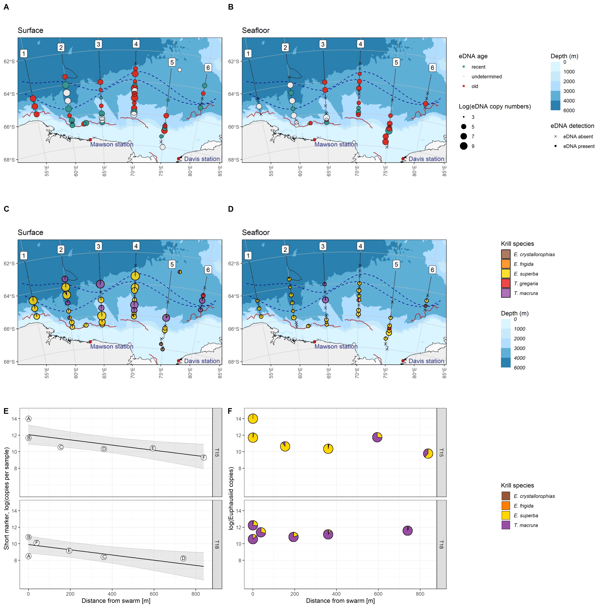
Top: Antarctic krill eDNA detected with the species-specific qPCR markers at CTD stations, in surface (A) and seafloor (B) samples. Colour denotes eDNA age estimated from DNA fragmentation, circle size corresponds to short marker copy numbers, dotted lines denote Southern Ocean oceanic fronts (see Figure 1) and red wavy lines indicate sea ice edge (see Figure 1). Middle: Krill species detected with the krill-specific metabarcoding marker at CTD stations, in surface (C) and seafloor (D) samples. Pie fractions correspond to metabarcoding read proportions within each sample, and circle size corresponds to estimates of overall krill eDNA abundance. Bottom: eDNA at two targeted krill swarms, T15 and T18. (E) Antarctic krill eDNA abundance measured with the species-specific markers significantly decreases with increasing distance from krill swarms, and overall at T18 significantly lower eDNA concentrations were detected than at T15. Letters within circles denote the order of sampling (at T18 the ship returned towards the swarm). (F) Krill species detected at increasing distance from krill swarms.
In CTD samples collected near the seafloor, substantially fewer samples contained Antarctic krill eDNA (29 out of 48, Figure 2B) than surface samples (44 out of 50, z = 2.985, p = 0.003, Figure 2A). eDNA abundance in seafloor samples was generally lower than in surface samples: apart from of one sample (3609 copies, recent), seafloor samples had less than 1000 copies (ranging from 20 to 955, median 158, Supplementary Figure S2). When compared to the surface, fewer samples were classified as recent, but a larger proportion of samples were classified as old in seafloor samples (seafloor: six recent, 15 old, eight undetermined, Figure 2B), however, due to small sample numbers, eDNA abundance and age patterns could not be formally assessed. Recent eDNA was generally detected further south near the continental slope, while older DNA was detected throughout the survey area. Antarctic krill eDNA was detected at great depth: nine detections were between 3000 m and 4000 m depth (one recent, six old, two undetermined age), four detections below 4000 m (one recent, one old, two undetermined age), with the deepest detection at 4327 m depth (undetermined age) and the deepest recent eDNA detection at 4300 m depth.
At two target trawl krill swarm locations (T15 and T18, Figure 1), eDNA was collected while the ship was positioned above the detected krill swarms (two samples each) and at several short intervals as the ship was moving away from/around the swarms. Preliminary analyses indicated that T15 likely falls into the ‘superswarm’ category, while T18 was of smaller, ‘standard swarm’ size (Tarling et al., 2009). While the ship was above these krill swarms, very high short marker copy numbers were detected (T15: 1,213,447 and 117,420 copies; T18: 49,360 and 4,428 copies) – higher than the highest copy numbers for any CTD samples at the surface (2,734 copies). The amount of eDNA significantly decreased with increasing distance from the swarms, and overall at T18 significantly lower eDNA concentrations were detected than at T15 (Figure 2E; Supplementary Table S2). At both swarm locations, the short marker copy numbers at the furthest distance measured from the swarm (T15: 837 m; T18: 739 m) was still greater than any surface detections from CTD samples (T15: 10,976 copies; T18: 3,730 copies). When the linear model was extrapolated to the lowest short marker copy number of any recent Antarctic krill eDNA detection (26 copies), the estimated distance at which the recent eDNA signal may still be detectable from a krill swarm was 2,794 m (T15) and 2,107 m (T18).
None of the negative PCR controls (36 NTC qPCRs) or the negative DNA extraction controls (54 qPCRs) amplified with either species-specific marker. Of the 11 field controls (66 qPCR amplifications), one qPCR amplification was positive. As only one of three technical replicas amplified, this control sample was still considered to be krill negative.
3.1.2 Euphausiid metabarcoding
Across all samples, five euphausiid species were detected: Euphausia superba, E. frigida Hansen, E. crystallorophias Holt & Tattersall, Thysanoessa macrura G.O. Sars and T. gregaria G.O. Sars. In the 50 CTD surface samples, predominantly two species were detected: E. superba (in 24 samples) and T. macrura (in 13 samples, Figure 2C). Traces of eDNA of E. frigida were found in one sample and of T. gregaria in two samples. The two southernmost samples in transect five (near 68°S) contained eDNA of E. crystallorophias.
In seafloor samples, predominantly E. superba was detected (25 samples), with traces of three other species present (T. macrura: three samples; T. gregaria: two samples; E. crystallorophias: one sample; Figure 2D). When estimates of semi-quantitative copy numbers were considered, generally less eDNA was detected in seafloor samples when compared to surface samples.
At the krill swarm locations where eDNA was sampled as the ship was moving away from the swarm, E. superba was the dominant krill species detected at swarm T15, however, at increasing distances from the swarm, substantial amounts of T. macrura eDNA were detected (Figure 2F, top). At swarm T18, only small proportions of reads were assigned to E. superba, while T. macrura was the dominant species detected (Figure 2F, bottom). At swarm T15, eDNA traces of E. crystallorophias (1 sample) and E. frigida (3 samples) were detected, while at swarm T18 eDNA traces of E. crystallorophias (1 sample) and E. frigida (4 samples) were detected.
3.1.3 Species-specific qPCR vs metabarcoding performance
There was a large overlap of samples where the species-specific assay (qPCR) and the metabarcoding assay both detected Antarctic krill eDNA (57 samples). However, in 30 additional samples, only the species-specific assay detected Antarctic krill eDNA (Supplementary Figure S3). These detections contained relatively low eDNA concentrations, and eDNA was often fragmented (26–861 copies; 20 samples old, six undetermined, four recent, see also Supplementary Figure S4A). In six samples, Antarctic krill eDNA was only detected with the metabarcoding marker (Supplementary Figure S3). The semi-quantitative estimate of metabarcoding copy numbers indicated that the eDNA concentrations in these samples was low for Antarctic krill (9–67 copies, median across all samples: 343 copies, see also Supplementary Figure S4B).
Antarctic krill eDNA copy numbers measured with the short species-specific marker positively correlated with copy numbers estimated from the metabarcoding assay, however, there was also a strong effect of sampling depth (Supplementary Table S3; Supplementary Figure S5), indicating that metabarcoding tended to overestimate the amount of Antarctic krill eDNA in surface samples, but not in seafloor samples, when compared to the species-specific marker.
3.2 Comparison to other methods
3.2.1 Acoustic
Acoustic detections of Antarctic krill across the survey area were previously reported in Cox et al. (2022) and are shown in Figure 3. Detection of acoustic biomass was best explained by the binomial generalized linear model that included terms for time of day and eDNA age class (decrease in AIC of 74.6 relative to the intercept-only model, Supplementary Table S4). Krill swarms were most likely to be detected around noon (Supplementary Figure S6). There was little evidence to suggest that adding distance (within the 15km limit) to this model further improved the fit (decrease in AIC of 1.4). Pairwise contrasts indicated that the probability of detecting acoustic biomass within 15 km of a “recent” eDNA sample (probability 0.35, averaged over the diel cycle) was significantly higher than for an “old” eDNA sample (probability 0.18; difference t(723) = 4.285, p < 0.001). The probability of detecting acoustic biomass within 15 km of an eDNA sample in which krill was not detected was 0.23, and this was not found to be significantly different from either “recent” or “old” eDNA samples (recent: t(723) = 2.303, p > 0.05; old: t(723) = 1.166, p > 0.05), but we note the low number (n = 6) of “no krill” eDNA samples.
Figure 3
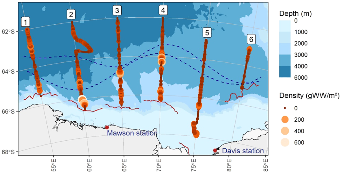
Acoustic measurement of Antarctic krill biomass. Circle size and colour denote areal density per nautical mile.
3.2.2 Visual
At surface CTD stations, Antarctic krill were visually detected at 18 out of 50 surveyed locations, largely south of the Polar Front, with some higher concentrations detected at the southern ends of transect two and three (Figure 4A). Antarctic krill eDNA was detected at every surface CTD station where Antarctic krill was visually detected (18 stations). In addition, Antarctic krill eDNA was also detected at 26 additional CTD surface locations where Antarctic krill was visually absent. At surface stations, there was no evidence that Antarctic krill eDNA abundance was associated with low or medium visual Antarctic krill abundance (likelihood ratio test 0.505, df = 1, p = 0.477, see also Supplementary Table S5). However, eDNA age was associated with visual detections: the probability of visually detecting medium krill abundances at surface stations was higher when the eDNA age was “recent” (likelihood ratio test 4.253, df = 1, p = 0.039, Supplementary Figure 7A).
Figure 4
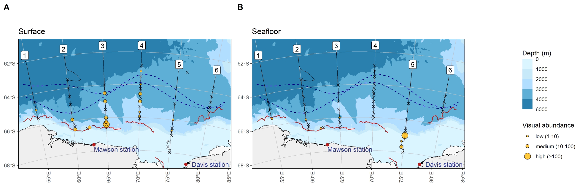
Top: Visual detection of Antarctic krill at the surface (A) and seafloor (B).
Similar to the pattern observed with eDNA, visual krill detections at the seafloor were less frequent (seven of 48 CTD station) than visual detections at the surface (18 out of 50 CTD stations, z = 2.365, p = 0.018, Figures 4A, B). The distribution of visual detections at depth was also similar to “recent” eDNA detections, i.e. concentrated at the southern end of the survey area (south of the Southern Boundary Front), near the continental slope (Figure 4B). Visual abundances at the seafloor were generally lower than at the surface, except for a krill swarm detected at the southern end of transect five at 381 m depth, where hundreds of Antarctic krill were caught on camera (Figure 4B; Supplementary Figure 7B) – the same location where exceptionally high concentrations of recent eDNA were detected (see above). Two visual detections were below 3000 m depth, with the deepest detection at 3080 m. At five of the seven visual detection locations, Antarctic krill eDNA was present. At one location (960 m depth, transect one), Antarctic krill eDNA was only detected with the metabarcoding assay, but not with the qPCR markers. At the deepest visual detection location (3080 m, transect three), eDNA was not detected with either method (qPCR or metabarcoding). At both those locations, visual krill abundance was low (1–10 krill, Supplementary Figure 7B). Antarctic krill eDNA was furthermore detected at 24 seafloor locations where visual detections were absent. There was not enough overlap between visual and eDNA detections at the seafloor to conduct meaningful statistical comparisons of eDNA abundance and age with visual abundance but see Supplementary Figure 7B for a visualization of the data.
3.2.3 Trawl
Krill densities (individuals per 1000 m3) were estimated for juvenile and adult krill from RMT 8 trawls, and for larval krill from RMT 1 trawls, at routine locations (pre-determined survey design; nRMT8 = 38; nRMT1 = 35) and at target locations (after acoustic detection of krill swarms; nRMT8 = 15; nRMT1 = 13). Similar to eDNA metabarcoding results, the most commonly detected juvenile/adult krill species across all RMT 8 trawls was E. superba (35 of 53 trawls, mean density of 281.91 krill per 1000 m3), followed by T. macrura (27 of 53 trawls, mean density 25.80 krill per 1000 m3, Supplementary Table S6). Results from RMT 8 trawls differed substantially between target and routine locations: At target trawls, E. superba was the dominant krill species: detected densities were higher than at routine trawl locations (Target trawls: mean density of 1023.75 krill per 1000 m3, Regular trawls: mean density of 28.99 per 1000 m3), and krill were detected more frequently (Target trawls: 14/15 locations, regular trawls: 21/38 locations, see Figures 5A, B; Supplementary Table S6). At regular trawls, other krill species were more commonly detected than at target trawls: T. macrura was detected at 25 locations throughout the survey area, E. crystallorophias at four southern locations and E. triacantha at eight northern/eastern locations (Figure 5A; Supplementary Table S6).
Figure 5
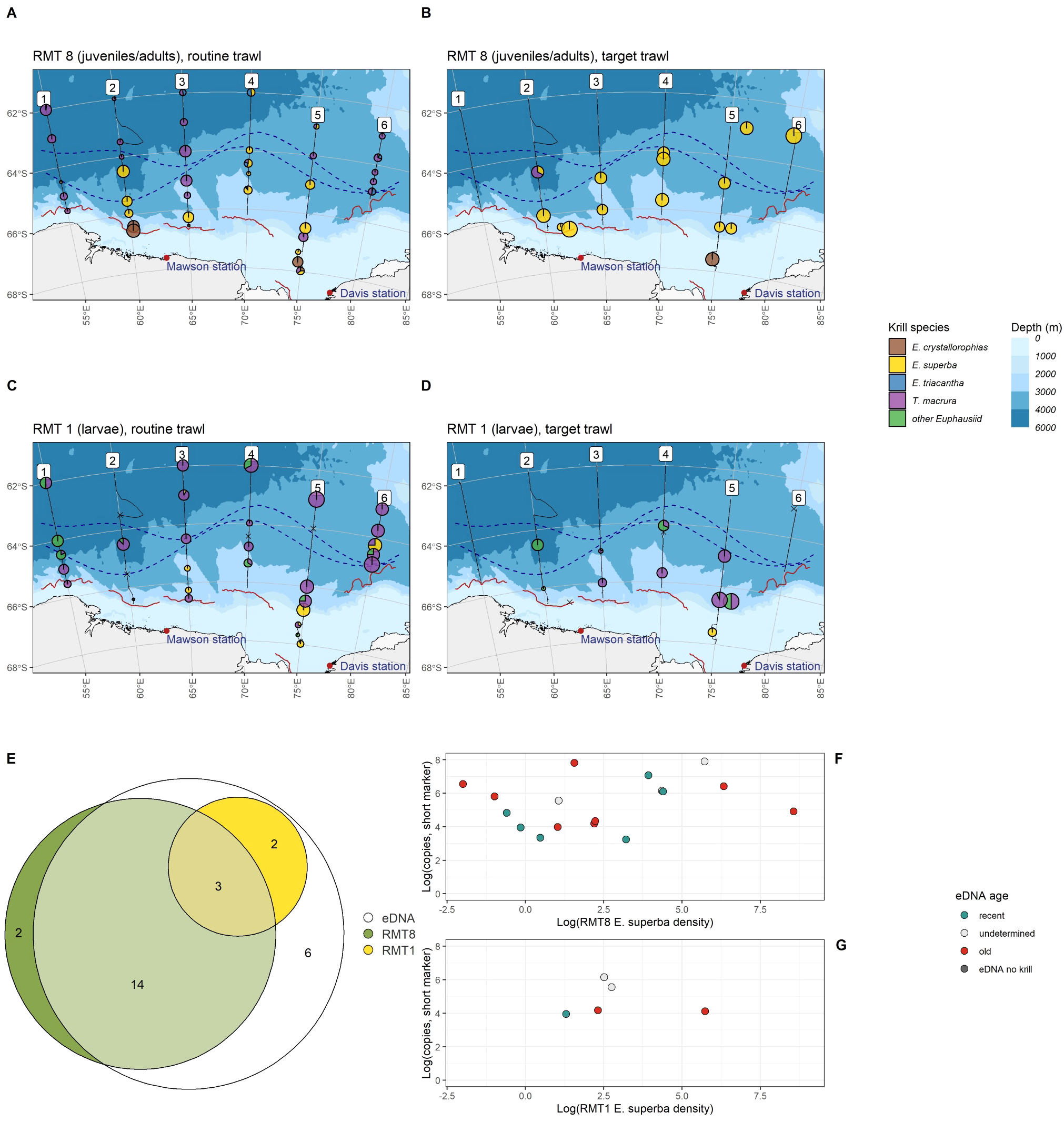
Top: Krill species (adults and juveniles) caught in RMT 8 trawls at routine (A) and target (B) trawl locations. Middle: Krill species (larvae) caught in RMT 1 trawls at routine (C) and target (D) trawl locations. Bottom: (E) overlap of Antarctic krill detections using species-specific eDNA amplification, RMT 8 trawls and RMT 1 trawls at locations where all three data types were collected. (F) eDNA age and abundance was not associated with juvenile/adult Antarctic krill density caught in RMT 8 trawls. (G) eDNA age and abundance did not correlate with Antarctic krill density of larval Antarctic krill caught in RMT 1 trawls.
Species detection patterns of RMT 1 trawl data (larval krill) differed both from RMT 8 (juvenile/adult) as well as eDNA metabarcoding data, however, there were no significant differences between routine and target trawl larval detections (Supplementary Table S7).Thysanoessa macrura was the most common euphausiid larval species, detected in 29 of 48 RMT 1 trawls throughout the survey area, both at routine and target locations, with an average density of 234.1 larvae per 1000 m3 (Figures 5C, D; Supplementary Table S7). Euphausia superba larvae were detected in nine of 48 RMT 1 trawls (both routine and target), and all detections were at the southern end of the survey area near the continental shelf (Figure 5B; Supplementary Table S7). Trawl results were further compared to eDNA results for trawls where both RMT 8 and RMT 1 data was successfully collected, and where a surface eDNA sample was collected from a CTD within 2,794 m distance. At most locations where juvenile/adult krill were present, and at all locations where larval krill were detected, Antarctic krill eDNA was also detected (19 of 21 and 5 of5, respectively, Figure 5E). In addition, Antarctic krill eDNA was also detected at six further locations where Antarctic krill was absent from trawls. Antarctic krill density from trawls did not correspond to eDNA abundance or eDNA age, neither for juvenile/adult krill (Figure 5F) nor for larval krill (Figure 5G).
4 Discussion
In this study we aimed to investigate whether eDNA-based methods can contribute to surveying Antarctic krill spatial and temporal distributions – crucial information for understanding Antarctic krill ecology and life history and the effects on and the krill-dependent ecosystem, but also important for the management of the Antarctic krill fishery. While eDNA methods have become more standardized and reliable over the last decade (Beng and Corlett, 2020; De Brauwer et al., 2023), understanding eDNA results, particularly in highly dynamic environments such as the Southern Ocean and for newly developed eDNA markers, requires careful comparisons to other survey methods (Burian et al., 2021). Here we compared two species-specific assays that can estimate Antarctic krill eDNA abundance and age, and a euphausiid-specific metabarcoding marker that can detect any Southern Ocean krill species, to three other krill survey methods (acoustic, visual, trawl), to gain a better understanding of krill eDNA properties in the Southern Ocean.
4.1 Surface
4.1.1 Antarctic krill
Antarctic krill eDNA was detected using species-specific qPCR assays (short and long marker) in most surface samples throughout the survey area. These results reflect that although Antarctic krill distribution is patchy in the Southern Ocean, krill swarms move around actively and with currents, and continuously release high concentrations of eDNA, for example through their molts and faeces. This eDNA can persist in the environment long after krill swarms have passed, and can spread further with currents, resulting in a nearly ubiquitous Antarctic krill eDNA presence in Southern Ocean surface waters, particularly of short eDNA fragments.
However, when eDNA abundance and eDNA age (estimated from eDNA fragmentation) were considered, a more diversified picture emerged: when eDNA samples were collected within or immediately above krill swarms, Antarctic krill eDNA concentrations were much higher than at other locations, reflecting the high eDNA shedding rates of dense krill swarms. With increasing distance to the swarms, eDNA concentrations declined at similar rates for both swarms. We estimated the distance at which recent eDNA shed from a krill swarm could still be detected to be up to approximately 2,794 m, however, as we did not collect samples beyond 800 m from the krill swarms, this estimate will need further examination with greater sampling density at greater distances from krill swarms, ideally also taking swarm size, krill density as well as the direction and strength of currents into account (Tarling et al., 2009; Andruszkiewicz et al., 2019). At T15, likely a very large ‘superswarm’, Antarctic krill eDNA concentrations were much higher than at T18, likely a smaller ‘standard swarm’, indicating that swarm size may relate to eDNA concentrations within the swarm. It is not yet clear whether Antarctic krill eDNA concentrations can provide quantitative information that would contribute to Antarctic krill biomass estimates across a survey area. However, as a first step, more frequent eDNA sampling along survey transects and further measurements of Antarctic krill eDNA concentrations within more krill swarms of different sizes would assist in characterizing the relationship between local biomass and eDNA concentrations.
Several aspects of our results suggested that recent eDNA detections indicated the presence of krill swarms nearby: in the vicinity (within 15 km) of recent eDNA detections, the probability of detecting krill swarms with acoustic surveys was greater than in the vicinity of old eDNA detections. In addition, higher visual krill abundance on video footage was related to more recent eDNA detections. In the acoustic data, the likelihood of detecting krill swarms was significantly higher around noon than other times of the day. This pattern is consistent with previous results from the same voyage in which krill densities during daytime were found to be higher than at night (Cox et al., 2022), and with results from other krill surveys of East Antarctica: during the BROKE-West voyage in 2006, lower krill densities were detected at night and krill surface swarms were visually detected during the day (Jarvis et al., 2010), and during the ENRICH voyage in 2019, more krill swarms were encountered during daytime around solar noon than during the night (Miller et al., 2019).
Based on the comparisons to the trawl data, Antarctic krill eDNA detections at the surface largely originated from juvenile or adult krill, with only a small proportion of the detections originating from larval krill. Larval Antarctic krill detections in trawls were restricted to the southern end of the survey, corresponding to the continental slope area, matching findings from Kawaguchi et al. (2010), who found larval krill distributions restricted to the shelf break.
4.1.2 Other euphausiids
For Antarctic krill surveys, metabarcoding of all krill species provided less differentiated data on Antarctic krill than the species-specific approach: the detection sensitivity was lower, eDNA abundance estimates were less reliable and eDNA fragmentation could not be measured (see also section 4.3). However, euphausiid metabarcoding was very useful to gain an understanding of the distribution, relative abundance and interaction of other krill species. In both eDNA metabarcoding and trawl data, E. superba was the most common species, followed by T. macrura, both following distribution and abundance expectations (Cuzin-Roudy et al., 2014). In RMT 8 trawls, E. superba densities and detection frequencies were significantly higher at target trawl locations than at regular trawl locations, reflecting the nature of the trawls: target trawls were conducted at locations where krill swarms (juvenile/adult krill) were acoustically detected, whereas regular trawls were conducted at pre-determined locations independent of acoustic presence of krill. The trawl type had no influence on the presence or abundance of other krill species, highlighting the specificity of acoustic krill swarm detections. While E. superba eDNA detections likely largely originated from juvenile/adult krill, a large proportion of T. macrura detections may have originated from larval krill: T. macrura was the most abundant larval krill species in RMT 1 trawls, matching findings of previous surveys (Hosie, 1991). Larval T. macrura were more abundant than adult T. macrura, and often co-occurred with adult E. superba. Thysanoessa macrura eDNA was also common around the two E. superba target swarms, and while we did not have RMT 1 trawl data for those locations due to net-opening failure, no adult T. macrura were detected there, thus the T. macrura eDNA likely originated from larvae.
In addition to these two dominant krill species, E. crystallorophias was detected in southernmost samples near the ice edge, the expected habitat of this species (Pakhomov and Perissinotto, 1996), both in eDNA samples (n = 2) and in trawls (n = 4). Traces of E. frigida eDNA were detected in one CTD sample and at both target swarms within the expected habitat (Hosie, 1991), and T. gregaria traces were found in two samples, outside of its expected more northerly range (Kirkwood, 1982). Neither E. frigida nor T. gregaria were detected in trawls, however, E. triacantha was detected in low densities in eight regular trawls, but not detected in eDNA samples. Mismatches between trawl and eDNA species detections could be related to the low densities/abundances of these species, or the mismatch of sampling depth (eDNA: surface; trawls: down to 200 m) or geographic location (CTD and trawl locations were up to 2.8 km apart). In addition, larval krill detections in trawls were only resolved to E. superba T. macrura and “other euphausiid”, thus other species detected with eDNA but not in trawls could have been present in un-identifiable larval form (compare to e.g. Hosie, 1991). Thysanoessa gregaria was the only krill species found outside its expected distribution range. Whether some T. gregaria individuals were lost in the South, whether their eDNA was carried south, e.g. through consumption by southwards moving predators (Reidy et al., 2022; Kawamura, 1980), or whether T. gregaria mitochondrial DNA introgressed into the T. macrura genome via the overlapping ranges of these closely related species (Qi et al., 2014; Seixas et al., 2018) requires further investigation.
4.2 Seafloor
4.2.1 Antarctic krill
Similar to surface samples, determining eDNA age in seafloor samples was essential to understand the presence and distribution of Antarctic krill in the seafloor environment: while low concentrations of Antarctic krill eDNA were detected throughout the survey area, recent eDNA detections were concentrated in the south at the continental slope area, only extending further north in transect two. Visual detections of Antarctic krill at the seafloor were also confined to the continental slope area, suggesting that recent eDNA detections in seafloor samples indicated the presence of Antarctic krill at depth. Recent eDNA detections towards the north of transect two may be related to different water properties discovered along this transect: Foppert et al. (2024) discovered higher dissolved oxygen and lower salinity at the seafloor along transect two, potentially related to an export pathway of Antarctic bottom water from the Cape Darnley Polynya through the Daly Canyon (Foppert et al., 2024). The exact relationship of krill at depth with Antarctic bottom water chemistry will require further in-depth investigation. Both recent eDNA and visual detections were found down to great depths, at 3080 m for the deepest visual detections, and at 4300 m for the deepest recent eDNA detections –considerably deeper than the deepest recorded presence of Antarctic krill to date (3500 m, Clarke and Tyler, 2008). The distribution of Antarctic krill at depth in the continental shelf area may be related to the seabed in this area providing an attractive and attainable alternative feeding ground for Antarctic krill (Schmidt et al., 2011). For example, phytodetritus can accumulate and persist on the continental shelf, providing a long-lasting food source for benthic feeders (Mincks et al., 2005; Smith et al., 2008). In times of relatively high predator abundance and low or patchy concentrations of phytoplankton in surface waters the seabed may present a preferable feeding ground for krill (Clarke and Tyler, 2008; Schmidt et al., 2011). Both individual and cooperative feeding behaviors have been described from benthic camera observations, from including the individual krill “skimming” the surface of the sediment to collect organic material to “balls” of krill resuspending sediment (Kane et al., 2021), and krill have been observed to excrete at depth, contributing to carbon export at depth as well as releasing eDNA into the environment (Smith et al., 2025). At one location at the southern end of transect five, an exceptionally large number of Antarctic krill were captured on camera (> 1000 krill at 381 m depth). At this location, the Antarctic krill eDNA concentration was the highest of any CTD sample (3609 copies), including surface samples, suggesting that high eDNA concentrations at depth corresponded to the presence of high krill numbers. In all other seafloor samples, Antarctic eDNA concentrations and visual krill densities were generally lower than in surface samples, suggesting that fewer Antarctic krill were present in the seafloor habitat, and/or krill were more spread out (generally not forming dense swarms at depth), resulting in lower eDNA concentrations at depth. The formation of dense krill swarms in the epipelagic zone is thought to be a mechanism to avoid visual predators (Olson et al., 2013) – in the darkness of the bathypelagic or even abyssopelagic zones swarming may be less useful to Antarctic krill, and individuals may spread out more at these depths.
Antarctic krill eDNA detections classified as “old” were spread throughout the survey area, including further north than recent detections. While these detections indicate the presence of Antarctic krill eDNA at depth, they may not necessarily indicate the presence of Antarctic krill, particularly beyond the continental slope: fecal pellets and molts released in great quantities by krill swarms in the epipelagic zone are known to sink (Cavan et al., 2019). While during the sinking process, particles may break up or be absorbed by microorganisms (Cavan et al., 2021), considerable amounts of krill debris may still reach the seafloor (Belcher et al., 2017; Smith et al., 2025), contributing to carbon export, and importantly carrying Antarctic krill eDNA to these depths. The sinking rate of krill fecal pellets is estimated to be 27–1218 m d−1 (median 304 m d−1) (Atkinson et al., 2012), and krill molts are estimated to sink at 52–1020 m d−1 (mean 674 m d−1) (Nicol and Stolp, 1989). To reach 3000 m depth, it could take 2.5–111 days (median 9.9 days) for fecal pellets, and 2.9–58 days (mean 5.5 days) for molts. During this sinking period the eDNA contained in the krill debris would likely fragment and reach the seafloor as “old” eDNA (Suter et al., 2023). Detection and quantification of old Antarctic krill eDNA could therefore indicate the amount and location of krill debris reaching the seafloor, which could contribute to estimates of krill-derived high-particulate organic carbon fluxes to the deep ocean (Manno et al., 2020).
4.2.2 Other euphausiids
The dominant euphausiid species detected in seafloor samples with the euphausiid-specific metabarcoding marker was E. superba. This likely reflects that of the detected krill species, E. superba is the only one known to descend to and actively inhabit the deep-sea environment. In addition, E. superba discarded matter may be more likely to reach the seafloor than the debris of other krill species: unlike other common Southern Ocean krill species (e.g. T. macrura), E. superba can form swarms of immense proportions. The generated localized large amounts of discarded krill matter may over-saturate scavenging communities, making it more likely for the discarded matter to reach the seafloor (Manno et al., 2020; Belcher et al., 2019). In addition, larger molts (such as adult E. superba molts) may sink faster than smaller molts (e.g. juvenile molts or molts of smaller euphausiid species such as T. macrura) (Nicol and Stolp, 1989), and molts can disintegrate within a few days, further reducing the likelihood of small molts reaching the seafloor (Nicol and Stolp, 1989).
4.3 Comparison of eDNA methods
When comparing Antarctic krill detections between eDNA methods (species-specific qPCR vs euphausiid-specific metabarcoding), the species-specific assay was more effective at detecting Antarctic krill eDNA, particularly at low eDNA concentrations and for old eDNA. This matches the findings of other studies (Yu et al., 2022; McColl-Gausden et al., 2023), where species-specific assays were also found to be more sensitive than metabarcoding assays. In the few instances where metabarcoding exclusively detected Antarctic krill eDNA, we estimated eDNA concentrations to be very low and potentially near or beyond the limit of detection for the species-specific markers. When we compared the eDNA amounts estimated for the metabarcoding data with species-specific qPCR eDNA amounts, the data matched very well, particularly for samples collected at the seafloor. However, metabarcoding tended to over-estimate the eDNA abundances for surface samples. For the semi-quantitative estimate of krill eDNA from metabarcoding data, Cq values from metabarcoding dye-based qPCRs were used (see methods). If surface samples contained non-euphausiid DNA that co-amplified in the krill metabarcoding assay, this could have contributed to lower Cq values and an over-estimation of total krill eDNA abundance. Resulting non-euphausiid sequences could subsequently have been removed during the library preparation or sequencing, or during the bioinformatic processing of the sequencing data, particularly if the off-target amplicon size differed from the krill amplicon size. If more reliable quantification of metabarcoding data were desired, this method would require further development, e.g. through addition of internal standards (Harrison et al., 2021), or through incorporation of euphausiid-specific fluorescent probes in the first-round metabarcoding qPCR instead of non-specific qPCR dye (Suter et al., 2023).
4.4 Comparison of different data types
Each eDNA survey method we attempted to integrate in this study had individual strengths and limitations (compare to Table 1). Data was collected at different intervals, with different geographic and temporal krill detection ranges (compare to Table 1) and targeting different developmental stages. For example, acoustic data was collected nearly continuously, with krill swarms (adult and juvenile) detectable to a depth of 250 m below the ship. In contrast, eDNA was only collected at CTD sampling stations from surface and seafloor waters, but eDNA could potentially detect the presence of krill (of any developmental stage) several kilometers away from the nearest krill swarm, and/or hours to days after a swarm had passed. Each data type provided a different angle on surveying Antarctic krill, and together the data provided a more holistic picture of Antarctic krill abundance and habitat use than either method could on its own.
Comparing the different data types not only helped interpret the eDNA data, but also expanded our geographic and temporal survey horizon. eDNA samples were comparatively simple to collect and could provide krill presence data beyond the immediate surroundings of the ship, including in areas that were otherwise hard to systematically sample by net or acoustics, such as the seafloor. Another area where eDNA but not many other data streams can be sampled is under sea ice, an important yet understudied habitat of Antarctic krill (Kawaguchi et al., 2024). In addition, eDNA metabarcoding data could also be used to optimize acoustic data interpretation in the future, for example by determining the species composition of krill swarms. Species compositions are traditionally assessed through trawls; however, krill swarms are often missed due to their high mobility and ability to avoid nets. eDNA on the other hand remains detectable for hours and could therefore be used more reliably to determine species compositions of swarms. Furthermore, eDNA samples also contain the DNA of any other organisms present in the sampled environment. Using a range of metabarcoding markers targeting taxonomic groups of interest could reveal the broader taxonomic community associated with krill swarms, ranging from diet species (phyto- and microzooplankton species) to krill predators (fish, marine mammals, seabirds), and could include any other species associated with krill swarms, including species commonly caught as bycatch by the krill fisheries (Stat et al., 2017; Krafft et al., 2023). Combining the eDNA-based krill survey method developed here with broader eDNA-based community assessments by using a suite of genetic markers on the same eDNA samples could therefore vastly improve our understanding of the entire trophic network connected to Antarctic krill.
5 Conclusions
This study is the first large-scale Southern Ocean survey that compared eDNA surveys of Antarctic krill and other euphausiids (species-specific qPCR assays to determine Antarctic krill eDNA abundance and age, and a euphausiid metabarcoding assay to detect all krill species) to other krill survey methods, including acoustic, visual and trawl surveys. Through these comparisons we gained new insights into Antarctic krill eDNA abundance, spread and decay in the dynamic Southern Ocean environment, interactions between krill species, and how eDNA based surveys could be used in the future to understand krill distributions and habitat use throughout the water column. We found that recent eDNA detections likely indicated the presence of Antarctic krill in the vicinity, both at the surface and at the seafloor. Very high eDNA abundances corresponded to the presence of krill swarms, but further studies are needed to interpret eDNA abundances more comprehensively. We recommend that future krill surveys integrate eDNA sampling throughout the water column in the survey design to complement other krill-related data streams. eDNA data can also expand our survey range to areas where other data streams cannot easily collect information, e.g. under sea ice or in the deep sea. Furthermore, eDNA samples could not only be used to assess Antarctic krill eDNA abundance and age but could also be used to assess other krill species, or indeed any taxonomic group of interest using targeted metabarcoding markers to expand our understanding of krill diet, interactions with other species and predator movements.
Statements
Data availability statement
The original contributions presented in the study are included in the article/Supplementary Material. Raw data and processing code are deposited on GitHub (https://github.com/AustralianAntarcticDivision/tempo-krill-comparisons) and on the Australian Antarctic Data Centre (https://data.aad.gov.au/metadata/AAS_4556_TEMPO_Euphausiid_metabarcoding_data). Further inquiries can be directed to the corresponding author/s.
Ethics statement
The manuscript presents research on animals that do not require ethical approval for their study.
Author contributions
LS: Conceptualization, Data curation, Formal Analysis, Investigation, Methodology, Project administration, Software, Validation, Visualization, Writing – original draft, Writing – review & editing. AB: Conceptualization, Data curation, Formal Analysis, Investigation, Methodology, Writing – original draft, Writing – review & editing. SB: Investigation, Writing – review & editing. JB: Investigation, Writing – review & editing. MB: Investigation, Writing – review & editing. MC: Data curation, Formal Analysis, Investigation, Methodology, Writing – original draft, Writing – review & editing. DH: Investigation, Writing – review & editing. OJ: Investigation, Writing – review & editing. SK: Conceptualization, Data curation, Formal Analysis, Funding acquisition, Investigation, Methodology, Project administration, Writing – review & editing. RK: Conceptualization, Investigation, Supervision, Writing – original draft, Writing – review & editing. AK: Investigation, Writing – review & editing. JM: Investigation, Supervision, Writing – review & editing. CW: Data curation, Formal Analysis, Investigation, Methodology, Writing – original draft, Writing – review & editing. SW: Conceptualization, Formal Analysis, Investigation, Writing – review & editing. BR: Conceptualization, Data curation, Formal Analysis, Investigation, Methodology, Validation, Writing – original draft, Writing – review & editing.
Funding
The author(s) declare that financial support was received for the research and/or publication of this article. Data collection and processing was funded by the Australian Antarctic Science Program (AAS 4556, AAS 4512, and AAS 4636). This project received grant funding from the Australian Government as part of the Antarctic Science Collaboration Initiative program. This project also received financial support from Pew Charitable Trust and Antarctic Science Foundation. We acknowledge the use of the CSIRO Marine National Facility (https://ror.org/01mae9353) and grant of sea time on RV Investigator in undertaking this research. AB was funded by an ARC Discovery Grant DP190100660 and the University of Sydney, Australia.
Acknowledgments
We thank Nat Kelly for designing the TEMPO survey, Gavin Macaulay, Dale Maschette and Abigail Smith for acoustic data collection, and Anna MacDonald, Andrea Polanowski and Abigail Smith for fruitful discussions. Thanks are also extended to the crew of the RV Investigator for their support throughout the voyage.
Conflict of interest
The authors declare that the research was conducted in the absence of any commercial or financial relationships that could be construed as a potential conflict of interest.
Generative AI statement
The author(s) declare that no Generative AI was used in the creation of this manuscript.
Publisher’s note
All claims expressed in this article are solely those of the authors and do not necessarily represent those of their affiliated organizations, or those of the publisher, the editors and the reviewers. Any product that may be evaluated in this article, or claim that may be made by its manufacturer, is not guaranteed or endorsed by the publisher.
Supplementary material
The Supplementary Material for this article can be found online at: https://www.frontiersin.org/articles/10.3389/fmars.2025.1502498/full#supplementary-material
References
1
Andruszkiewicz E. A. Koseff J. R. Fringer O. B. Ouellette N. T. Lowe A. B. Edwards C. A. et al . (2019). Modeling environmental DNA transport in the coastal ocean using Lagrangian particle tracking. Front. Marine Sci.6, 477. doi: 10.3389/fmars.2019.00477
2
Atkinson A. Hill S. L. Pakhomov E. A. Siegel V. Reiss C. S. Loeb V. J. et al . (2019). Krill (Euphausia superba) distribution contracts southward during rapid regional warming. Nat. Climate Change9, 142–147. doi: 10.1038/s41558-018-0370-z
3
Atkinson A. Schmidt K. Fielding S. Kawaguchi S. Geissler P. A. (2012). Variable food absorption by Antarctic krill: Relationships between diet, egestion rate and the composition and sinking rates of their fecal pellets. Deep Sea Res. Part II: Topical Stud. Oceanogr.59-60, 147–158. doi: 10.1016/j.dsr2.2011.06.008
4
Atkinson A. Siegel V. Pakhomov E. A. Jessopp M. J. Loeb V. (2009). A re-appraisal of the total biomass and annual production of Antarctic krill. Deep Sea Res. (Part I Oceanogr. Res. Pap.)56, 727–740. doi: 10.1016/j.dsr.2008.12.007
5
Atkinson A. Siegel V. Pakhomov E. Rothery P. (2004). Long-term decline in krill stock and increase in salps within the Southern Ocean. Nature432, 100–103. doi: 10.1038/nature02996
6
Atkinson A. Siegel V. Pakhomov E. A. Rothery P. Loeb V. Ross R. M. et al . (2008). Oceanic circumpolar habitats of Antarctic krill. Marine Ecol. Prog. Ser.362, 1–23. doi: 10.3354/meps07498
7
Bahlburg D. Hüppe L. Böhrer T. Thorpe S. E. Murphy E. J. Berger U. et al . (2023). Plasticity and seasonality of the vertical migration behaviour of Antarctic krill using acoustic data from fishing vessels. R. Soc. Open Sci.10, 230520. doi: 10.1098/rsos.230520
8
Baldo L. Dunning Hotopp J. C. Jolley K. A. Bordenstein S. R. Biber S. A. Choudhury R. R. et al . (2006). Multilocus sequence typing system for the endosymbiont Wolbachia pipientis. Appl. Environ. Microbiol.72, 7098–7110. doi: 10.1128/AEM.00731-06
9
Belcher A. Henson S. Manno C. Hill S. Atkinson A. Thorpe S. et al . (2019). Krill faecal pellets drive hidden pulses of particulate organic carbon in the marginal ice zone. Nat. Commun.10, 889. doi: 10.1038/s41467-019-08847-1
10
Belcher A. Tarling G. Manno C. Atkinson A. Ward P. Skaret G. et al . (2017). The potential role of Antarctic krill faecal pellets in efficient carbon export at the marginal ice zone of the South Orkney Islands in spring. Polar Biol.40, 2001–2013. doi: 10.1007/s00300-017-2118-z
11
Beng K. C. Corlett R. T. (2020). Applications of environmental DNA (eDNA) in ecology and conservation: opportunities, challenges and prospects. Biodivers. Conserv.29, 2089–2121. doi: 10.1007/s10531-020-01980-0
12
Berry T. E. Osterrieder S. K. Murray D. C. Coghlan M. L. Richardson A. J. Grealy A. K. et al . (2017). DNA metabarcoding for diet analysis and biodiversity: A case study using the endangered Australian sea lion (Neophoca cinerea). Ecol. Evol.7, 5435–5453. doi: 10.1002/ece3.2017.7.issue-14
13
Bessey C. Jarman S. N. Berry O. Olsen Y. S. Bunce M. Simpson T. et al . (2020). Maximizing fish detection with eDNA metabarcoding. Environ. DNA2, 493–504. doi: 10.1002/edn3.v2.4
14
Burian A. Mauvisseau Q. Bulling M. Domisch S. Qian S. Sweet M. (2021). Improving the reliability of eDNA data interpretation. Mol. Ecol. Resour.21, 1422–1433. doi: 10.1111/1755-0998.13367
15
Bylemans J. Furlan E. M. Gleeson D. M. Hardy C. M. Duncan R. P. (2018). Does size matter? An experimental evaluation of the relative abundance and decay rates of aquatic environmental DNA. Environ. Sci. Technol.52, 6408–6416. doi: 10.1021/acs.est.8b01071
16
Campbell M. D. Pollack A. G. Gledhill C. T. Switzer T. S. Devries D. A. (2015). Comparison of relative abundance indices calculated from two methods of generating video count data. Fish. Res.170, 125–133. doi: 10.1016/j.fishres.2015.05.011
17
Cavan E. Belcher A. Atkinson A. Hill S. Kawaguchi S. Mccormack S. et al . (2019). The importance of Antarctic krill in biogeochemical cycles. Nat. Commun.10, 4742. doi: 10.1038/s41467-019-12668-7
18
Cavan E. L. Kawaguchi S. Boyd P. W. (2021). Implications for the mesopelagic microbial gardening hypothesis as determined by experimental fragmentation of Antarctic krill fecal pellets. Ecol. Evol.11, 1023–1036. doi: 10.1002/ece3.v11.2
19
Cavanagh R. D. Melbourne-Thomas J. Grant S. M. Barnes D. K. Hughes K. A. Halfter S. et al . (2021). Future risk for Southern Ocean ecosystem services under climate change. Front. Marine Sci.7, 615214. doi: 10.3389/fmars.2020.615214
20
Clarke L. J. Shaw J. D. Suter L. Atalah J. Bergstrom D. M. Biersma E. et al . (2023). An expert-driven framework for applying eDNA tools to improve biosecurity in the Antarctic. Manage. Biol. Invasions14, 379–402. doi: 10.3391/mbi.2023.14.3.01
21
Clarke A. Tyler P. A. (2008). Adult antarctic krill feeding at abyssal depths. Curr. Biol.18, 282–285. doi: 10.1016/j.cub.2008.01.059
22
Constable A. J. Nicol S. (2002). Defining smaller-scale management units to further develop the ecosystem approach in managing large-scale pelagic krill fisheries in Antarctica. Ccamlr Sci.9, 117–131.
23
Cox M. J. Candy S. de la Mare W. K. Nicol S. Kawaguchi S. Gales N. (2018). No evidence for a decline in the density of Antarctic krill Euphausia superba Dana 1850, in the Southwest Atlantic sector between 1976 and 2016. J. Crustacean Biol.38, 656–661. doi: 10.1093/jcbiol/ruy072
24
Cox M. J. Macaulay G. Brasier M. J. Burns A. Johnson O. J. King R. et al . (2022). Two scales of distribution and biomass of Antarctic krill (Euphausia superba) in the eastern sector of the CCAMLR Division 58.4. 2 (55 E to 80 E). PloS One17, e0271078. doi: 10.1371/journal.pone.0271078
25
Cox M. J. Watkins J. L. Reid K. Brierley A. S. (2011). Spatial and temporal variability in the structure of aggregations of Antarctic krill (Euphausia superba) around South Georgia 1997–1999. ICES J. Marine Sci.68, 489–498. doi: 10.1093/icesjms/fsq202
26
Cutter G. R. Jr. Reiss C. S. Nylund S. Watters G. M. (2022). Antarctic krill biomass and flux measured using wideband echosounders and acoustic Doppler current profilers on submerged moorings. Front. Marine Sci.9, 784469. doi: 10.3389/fmars.2022.784469
27
Cuzin-Roudy J. Irisson J.-O. Penot F. Kawaguchi S. Vallet C. (2014). 6.9. Southern Ocean Euphausiids. (Cambridge, United Kingdom: Scientific Committee on Antarctic Research).
28
De Brauwer M. Clarke L. J. Chariton A. Cooper M. K. De Bruyn M. Furlan E. et al . (2023). Best practice guidelines for environmental DNA biomonitoring in Australia and New Zealand. Environ. DNA5, 417–423. doi: 10.1002/edn3.395
29
Deiner K. Bik H. M. Mächler E. Seymour M. Lacoursière-Roussel A. Altermatt F. et al . (2017). Environmental DNA metabarcoding: Transforming how we survey animal and plant communities. Mol. Ecol.26, 5872–5895. doi: 10.1111/mec.2017.26.issue-21
30
De Ronde M. W. Ruijter J. M. Lanfear D. Bayes-Genis A. Kok M. G. Creemers E. E. et al . (2017). Practical data handling pipeline improves performance of qPCR-based circulating miRNA measurements. Rna23, 811–821. doi: 10.1261/rna.059063.116
31
Dugal L. Thomas L. Meenakshisundaram A. Simpson T. Lines R. Colquhoun J. et al . (2023). Distinct coral reef habitat communities characterized by environmental DNA metabarcoding. Coral Reefs42, 17–30. doi: 10.1007/s00338-022-02301-3
32
Edgar R. C. (2010). Search and clustering orders of magnitude faster than BLAST. Bioinformatics26, 2460–2461. doi: 10.1093/bioinformatics/btq461
33
Ellis M. R. Clark Z. S. Treml E. A. Brown M. S. Matthews T. G. Pocklington J. B. et al . (2022). Detecting marine pests using environmental DNA and biophysical models. Sci. Total Environ.816, 151666. doi: 10.1016/j.scitotenv.2021.151666
34
Everson I. (2008). Krill: biology, ecology and fisheries (John Wiley & Sons).
35
Fielding S. Watkins J. L. Trathan P. N. Enderlein P. Waluda C. M. Stowasser G. et al . (2014). Interannual variability in Antarctic krill (Euphausia superba) density at South Georgia, Southern Ocean: 1997-2013. ICES J. Marine Sci.71, 2578–2588. doi: 10.1093/icesjms/fsu104
36
Flores H. Atkinson A. Kawaguchi S. Krafft B. A. Milinevsky G. Nicol S. et al . (2012). Impact of climate change on Antarctic krill. Marine Ecol. Prog. Ser.458, 1–19. doi: 10.3354/meps09831
37
Foppert A. Bestley S. Shadwick E. H. Klocker A. Vives C. R. Liniger G. et al . (2024). Observed water-mass characteristics and circulation off Prydz Bay, East Antarctica. Front. Marine Sci.11, 1456207. doi: 10.3389/fmars.2024.1456207
38
French B. Wilson S. Holmes T. Kendrick A. Rule M. Ryan N. (2021). Comparing five methods for quantifying abundance and diversity of fish assemblages in seagrass habitat. Ecol. Indic.124, 107415. doi: 10.1016/j.ecolind.2021.107415
39
Gardner J. Struthers C. (2013). Comparisons among survey methodologies to test for abundance and size of a highly targeted fish species. J. Fish Biol.82, 242–262. doi: 10.1111/j.1095-8649.2012.03478.x
40
Gargan L. M. Morato T. Pham C. K. Finarelli J. A. Carlsson J. E. Carlsson J. (2017). Development of a sensitive detection method to survey pelagic biodiversity using eDNA and quantitative PCR: a case study of devil ray at seamounts. Marine Biol.164, 1–9. doi: 10.1007/s00227-017-3141-x
41
Gleiber M. R. Steinberg D. K. Ducklow H. W. (2012). Time series of vertical flux of zooplankton fecal pellets on the continental shelf of the western Antarctic Peninsula. Marine Ecol. Prog. Ser.471, 23–36. doi: 10.3354/meps10021
42
Harrison J. G. John Calder W. Shuman B. Alex Buerkle C. (2021). The quest for absolute abundance: The use of internal standards for DNA-based community ecology. Mol. Ecol. Resour.21, 30–43. doi: 10.1111/1755-0998.13247
43
Hewitt R. P. Watkins J. Naganobu M. Sushin V. Brierley A. S. Demer D. et al . (2004). Biomass of Antarctic krill in the Scotia Sea in January/February 2000 and its use in revising an estimate of precautionary yield. Deep Sea Research Part II: Topical Studies in Oceanography. 51 (12-13), 1215–36. doi: 10.1016/j.dsr2.2004.06.011
44
Hill S. L. (2013). Prospects for a sustainable increase in the availability of long chain omega 3s: lessons from the Antarctic krill fishery. Omega-6/3 Fatty Acids: Functions, Sustainability Strategies and Perspectives. (Totowa, NJ: Humana Press), 267–296. doi: 10.1007/978-1-62703-215-5_14
45
Hosie G. (1991). Distribution and abundance of euphausiid larvae in the Prydz Bay region, Antarctica. Antarctic Sci.3, 167–180. doi: 10.1017/S0954102091000202
46
Huson D. H. Beier S. Flade I. Górska A. El-Hadidi M. Mitra S. et al . (2016). MEGAN community edition-interactive exploration and analysis of large-scale microbiome sequencing data. PloS Comput. Biol.12, e1004957. doi: 10.1371/journal.pcbi.1004957
47
Jarman S. N. Berry O. Bunce M. (2018). The value of environmental DNA biobanking for long-term biomonitoring. Nat. Ecol. Evol.2, 1192. doi: 10.1038/s41559-018-0614-3
48
Jarvis T. Kelly N. Kawaguchi S. Van Wijk E. Nicol S. (2010). Acoustic characterisation of the broad-scale distribution and abundance of Antarctic krill (Euphausia superba) off East Antarctica (30–80 E) in January-March 2006. Deep Sea Res. Part II: Topical Stud. Oceanogr.57, 916–933. doi: 10.1016/j.dsr2.2008.06.013
49
Jeunen G. J. Knapp M. Spencer H. G. Lamare M. D. Taylor H. R. Stat M. et al . (2019). Environmental DNA (eDNA) metabarcoding reveals strong discrimination among diverse marine habitats connected by water movement. Mol. Ecol. Resour.19, 426–438. doi: 10.1111/men.2019.19.issue-2
50
Jo T. Murakami H. Masuda R. Sakata M. K. Yamamoto S. Minamoto T. (2017). Rapid degradation of longer DNA fragments enables the improved estimation of distribution and biomass using environmental DNA. Mol. Ecol. Resour.17, e25–e33. doi: 10.1111/men.2017.17.issue-6
51
Kalinowski J. Witek Z. (1980). Diurnal vertical distribution of krill aggregations in the Western Antarctic. Polish Polar Res.1, 127–146.
52
Kane M. K. Atkinson A. Menden-Deuer S. (2021). Lowered cameras reveal hidden behaviors of Antarctic krill. Curr. Biol.31, R237–R238. doi: 10.1016/j.cub.2021.01.091
53
Kawaguchi S. Atkinson A. Bahlburg D. Bernard K. S. Cavan E. L. Cox M. J. et al . (2024). Climate change impacts on Antarctic krill behaviour and population dynamics. Nat. Rev. Earth Environ.5, 43–58. doi: 10.1038/s43017-023-00504-y
54
Kawaguchi S. Nicol S. (2020). Krill fishery. Fish. Aquac.9, 137–158. doi: 10.1093/oso/9780190865627.003.0006
55
Kawaguchi S. Nicol S. Virtue P. Davenport S. R. Casper R. Swadling K. M. et al . (2010). Krill demography and large-scale distribution in the Western Indian Ocean sector of the Southern Ocean (CCAMLR Division 58.4.2) in Austral summer of 2006. Deep Sea Res. Part II: Topical Stud. Oceanogr.57, 934–947. doi: 10.1016/j.dsr2.2008.06.014
56
Kawamura A. (1980). A review of food of balaenopterid whales. Sci. Rep. Whales Res. Inst32, 155–197.
57
Kils U. (1982). The swimming behavior, swimming performance, and energy balance of Antarctic krill, Euphausia superba (Cambridge: SCAR).
58
Kirkwood J. M. (1982). “A guide to the Euphausiacea of the Southern Ocean,” in ANARE Research Notes (Kingston, Tasmania, Australia: Australian Antarctic Division).
59
Klymus K. E. Merkes C. M. Allison M. J. Goldberg C. S. Helbing C. C. Hunter M. E. et al . (2020a). Reporting the limits of detection and quantification for environmental DNA assays. Environ. DNA2, 271–282. doi: 10.1002/edn3.v2.3
60
Klymus K. E. Ramos D. V. R. Thompson N. L. Richter C. A. (2020b). Development and testing of species-specific quantitative PCR assays for environmental DNA applications. JoVE (Journal Visualized Experiments)165, e61825. doi: 10.3791/61825
61
Krafft B. A. Lowther A. Krag L. A. (2023). Bycatch in the Antarctic krill (Euphausia superba) trawl fishery. Fish. Manage. Ecol.30, 154–160. doi: 10.1111/fme.12607
62
Krafft B. A. Macaulay G. J. Skaret G. Knutsen T. Bergstad O. A. Lowther A. et al . (2021). Standing stock of Antarctic krill (Euphausia superba Dana 1850)(Euphausiacea) in the Southwest Atlantic sector of the Southern Ocean 2018–19. J. Crustacean Biol.41, 1–17. doi: 10.1093/jcbiol/ruab071
63
Lacoursière-Roussel A. Côté G. Leclerc V. Bernatchez L. (2016). Quantifying relative fish abundance with eDNA: a promising tool for fisheries management. J. Appl. Ecol.53, 1148–1157. doi: 10.1111/1365-2664.12598
64
Langlois V. S. Allison M. J. Bergman L. C. To T. A. Helbing C. C. (2021). The need for robust qPCR-based eDNA detection assays in environmental monitoring and species inventories. Environ. DNA3, 519–527. doi: 10.1002/edn3.v3.3
65
Larsson J. (2020). eulerr: Area-Proportional Euler and Venn Diagrams with Ellipses. R package version 7.0.2. Available online at: https://CRAN.R-project.org/package=eulerr.
66
LeBlanc F. Belliveau V. Watson E. Coomber C. Simard N. Dibacco C. et al . (2020). Environmental DNA (eDNA) detection of marine aquatic invasive species (AIS) in Eastern Canada using a targeted species-specific qPCR approach. Manage. Biol. Invasions11, 201–217. doi: 10.3391/mbi.2020.11.2.03
67
Lenth R. (2024). emmeans: Estimated Marginal Means, aka Least-Squares Means. R package version 1.10.3. Available online at: https://CRAN.R-project.org/package=emmeans.
68
Luo M. Ji Y. Douglas W. Y. (2022). Extracting abundance information from DNA-based data. Molecular Ecology Resources. 23 (1), 174–89. doi: 10.1111/1755-0998.13703
69
MacLennan D. N. Fernandes P. G. Dalen J. (2002). A consistent approach to definitions and symbols in fisheries acoustics. ICES J. Marine Sci.59, 365–369. doi: 10.1006/jmsc.2001.1158
70
Madden T. (2013). “The BLAST sequence analysis tool,” in The NCBI Handbook, 2nd edition (National Center for Biotechnology Information (US, Bethesda (MD).
71
Manno C. Fielding S. Stowasser G. Murphy E. Thorpe S. Tarling G. (2020). Continuous moulting by Antarctic krill drives major pulses of carbon export in the north Scotia Sea, Southern Ocean. Nat. Commun.11, 6051. doi: 10.1038/s41467-020-19956-7
72
Maschette D. Sumner M. Raymond B. (2019). SOmap: Southern Ocean maps. Available online at: https://github.com/AustralianAntarcticDivision/SOmap.
73
Mathon L. Marques V. Mouillot D. Albouy C. Andrello M. Baletaud F. et al . (2022). Cross-ocean patterns and processes in fish biodiversity on coral reefs through the lens of eDNA metabarcoding. Proc. R. Soc. B.289, 20220162. doi: 10.1098/rspb.2022.0162
74
McColl-Gausden E. F. Weeks A. R. Coleman R. Song S. Tingley R. (2023). Using hierarchical models to compare the sensitivity of metabarcoding and qPCR for eDNA detection. Ecol. Inf.75, 102072. doi: 10.1016/j.ecoinf.2023.102072
75
Meyer B. Freier U. Grimm V. Groeneveld J. Hunt B. P. Kerwath S. et al . (2017). The winter pack-ice zone provides a sheltered but food-poor habitat for larval Antarctic krill. Nat. Ecol. Evol.1, 1853–1861. doi: 10.1038/s41559-017-0368-3
76
Miller D. Agnew D. (2000). Management of krill fisheries in the Southern Ocean. Krill Biol. Ecol. Fish., 300–337. doi: 10.1002/9780470999493
77
Miller E. Potts J. Cox M. Miller B. Calderan S. Leaper R. et al . (2019). The characteristics of krill swarms in relation to aggregating Antarctic blue whales. Sci. Rep.9, 16487. doi: 10.1038/s41598-019-52792-4
78
Mincks S. L. Smith C. R. Demaster D. J. (2005). Persistence of labile organic matter and microbial biomass in Antarctic shelf sediments: evidence of a sediment ‘food bank’. Marine Ecol. Prog. Ser.300, 3–19. doi: 10.3354/meps300003
79
Miya M. (2022). Environmental DNA Metabarcoding: A novel method for biodiversity monitoring of marine fish communities. Annu. Rev. Marine Sci.14, 161–185. doi: 10.1146/annurev-marine-041421-082251
80
Morgan M. Anders S. Lawrence M. Aboyoun P. Pages H. Gentleman R. (2009). ShortRead: a bioconductor package for input, quality assessment and exploration of high-throughput sequence data. Bioinformatics25, 2607–2608. doi: 10.1093/bioinformatics/btp450
81
Motoda S. (1985). Devices of simple plankton apparatus VII. Bull. Mar. Sci.37, 776–777.
82
Nester G. Suter L. Kitchener J. Bunce M. Polanowski A. Wasserman J. et al . (2024). Long-distance Southern Ocean environmental DNA (eDNA) transect provides insights into spatial marine biota and invasion pathways for non-native species. Authorea Preprints. 951, 175657. doi: 10.1016/j.scitotenv.2024.175657
83
Nicol S. Stolp M. (1989). Sinking rates of cast exoskeletons of Antarctic krill (Euphausia superba Dana) and their role in the vertical flux of particulate matter and fluoride in the Southern Ocean. Deep Sea Res. Part A. Oceanogr. Res. Pap.36, 1753–1762. doi: 10.1016/0198-0149(89)90070-8
84
Olson R. S. Hintze A. Dyer F. C. Knoester D. B. Adami C. (2013). Predator confusion is sufficient to evolve swarming behaviour. J. R. Soc. Interface10, 20130305. doi: 10.1098/rsif.2013.0305
85
Pakhomov E. Perissinotto R. (1996). Antarctic neritic krill Euphausia crystallorophias: spatio-temporal distribution, growth and grazing rates. Deep Sea Res. Part I: Oceanogr. Res. Pap.43, 59–87. doi: 10.1016/0967-0637(95)00094-1
86
Pelletier D. Leleu K. Mou-Tham G. Guillemot N. Chabanet P. (2011). Comparison of visual census and high definition video transects for monitoring coral reef fish assemblages. Fish. Res.107, 84–93. doi: 10.1016/j.fishres.2010.10.011
87
Qi Y. Lu B. Gao H. Hu P. Fu J. (2014). Hybridization and mitochondrial genome introgression between Rana chensinensis and R. kukunoris. Mol. Ecol.23, 5575–5588. doi: 10.1111/mec.2014.23.issue-22
88
Reidy R. D. Lemay M. A. Innes K. G. Clemente-Carvalho R. B. Janusson C. Dower J. F. et al . (2022). Fine-scale diversity of prey detected in humpback whale feces. Ecol. Evol.12, e9680. doi: 10.1002/ece3.v12.12
89
Reiss C. S. Cossio A. M. Loeb V. Demer D. A. (2008). Variations in the biomass of Antarctic krill (Euphausia superba) around the South Shetland Islands 1996–2006. ICES J. Marine Sci.65, 497–508. doi: 10.1093/icesjms/fsn033
90
Richerson K. Watters G. M. Santora J. A. Schroeder I. D. Mangel M. (2015). More than passive drifters: a stochastic dynamic model for the movement of Antarctic krill. Marine Ecol. Prog. Ser.529, 35–48. doi: 10.3354/meps11324
91
Rourke M. L. Fowler A. M. Hughes J. M. Broadhurst M. K. Dibattista J. D. Fielder S. et al . (2022). Environmental DNA (eDNA) as a tool for assessing fish biomass: A review of approaches and future considerations for resource surveys. Environ. DNA4, 9–33. doi: 10.1002/edn3.185
92
Roux L. M. D. Giblot-Ducray D. Bott N. J. Wiltshire K. H. Deveney M. R. Westfall K. M. et al . (2020). Analytical validation and field testing of a specific qPCR assay for environmental DNA detection of invasive European green crab (Carcinus maenas). Environ. DNA2, 309–320. doi: 10.1002/edn3.v2.3
93
Ruppert K. M. Kline R. J. Rahman M. S. (2019). Past, present, and future perspectives of environmental DNA (eDNA) metabarcoding: A systematic review in methods, monitoring, and applications of global eDNA. Global Ecol. Conserv.17, e00547. doi: 10.1016/j.gecco.2019.e00547
94
Salter I. Joensen M. Kristiansen R. Steingrund P. Vestergaard P. (2019). Environmental DNA concentrations are correlated with regional biomass of Atlantic cod in oceanic waters. Commun. Biol.2, 461. doi: 10.1038/s42003-019-0696-8
95
Schmidt K. Atkinson A. (2016). Feeding and food processing in Antarctic krill (Euphausia superba Dana). Biol. Ecol. Antarctic krill, 175–224. doi: 10.1007/978-3-319-29279-3_5
96
Schmidt K. Atkinson A. Steigenberger S. Fielding S. Lindsay M. C. Pond D. W. et al . (2011). Seabed foraging by Antarctic krill: Implications for stock assessment, bentho-pelagic coupling, and the vertical transfer of iron. Limnol. Oceanogr.56, 1411–1428. doi: 10.4319/lo.2011.56.4.1411
97
Schobernd Z. H. Bacheler N. M. Conn P. B. (2014). Examining the utility of alternative video monitoring metrics for indexing reef fish abundance. Can. J. Fish. Aquat. Sci.71, 464–471. doi: 10.1139/cjfas-2013-0086
98
Seixas F. A. Boursot P. Melo-Ferreira J. (2018). The genomic impact of historical hybridization with massive mitochondrial DNA introgression. Genome Biol.19, 1–20. doi: 10.1186/s13059-018-1471-8
99
Siegel V. (2016). “Introducing Antarctic krill Euphausia superba Dana 1850,” in Biology and Ecology of Antarctic Krill (Switzerland: Springer).
100
Skaret G. Macaulay G. Pedersen R. Wang X. Klevjer T. A. Krag L. et al . (2023). Distribution and biomass estimation of Antarctic krill (Euphausia superba) off the South Orkney Islands during 2011–2020. ICES J. Marine Sci.80, 1472–1486. doi: 10.1093/icesjms/fsad076
101
Smith C. R. Mincks S. Demaster D. J. (2008). The FOODBANCS project: introduction and sinking fluxes of organic carbon, chlorophyll-a and phytodetritus on the western Antarctic Peninsula continental shelf. Deep Sea Res. Part II: Topical Stud. Oceanogr.55, 2404–2414. doi: 10.1016/j.dsr2.2008.06.001
102
Smith A. Wotherspoon S. Ratnarajah L. Cutter G. Macaulay G. Hutton B. et al . (2025). Antarctic krill vertical migrations modulate seasonal carbon export. Science387, eadq5564. doi: 10.1126/science.adq5564
103
Stat M. Huggett M. J. Bernasconi R. Dibattista J. D. Berry T. E. Newman S. J. et al . (2017). Ecosystem biomonitoring with eDNA: metabarcoding across the tree of life in a tropical marine environment. Sci. Rep.7, 1–11. doi: 10.1038/s41598-017-12501-5
104
Suter L. Polanowski A. M. Clarke L. J. Kitchener J. A. Deagle B. E. (2021). Capturing open ocean biodiversity: Comparing environmental DNA metabarcoding to the continuous plankton recorder. Mol. Ecol.30, 3140–3157. doi: 10.1111/mec.v30.13
105
Suter L. Wotherspoon S. Kawaguchi S. King R. Macdonald A. J. Nester G. M. et al . (2023). Environmental DNA of Antarctic krill (Euphausia superba): Measuring DNA fragmentation adds a temporal aspect to quantitative surveys. Environ. DNA5, 945–959. doi: 10.1002/edn3.v5.5
106
Suter L . (2025). Euphausiid-specific metabarcoding data from eDNA samples and video footage collected on the TEMPO voyage, Ver. 1, Australian Antarctic Data Centre -. doi: 10.26179/hr9a-jv26
107
Taberlet P. Bonin A. Zinger L. Coissac E. (2018). Environmental DNA: For Biodiversity Research and Monitoring (Oxford UK: Oxford University Press).
108
Tarling G. A. Fielding S. (2016). “Swarming and behaviour in Antarctic krill,” in Biology and Ecology of Antarctic Krill (Switzerland: Springer).
109
Tarling G. A. Klevjer T. Fielding S. Watkins J. Atkinson A. Murphy E. et al . (2009). Variability and predictability of Antarctic krill swarm structure. Deep Sea Res. Part I: Oceanogr. Res. Pap.56, 1994–2012. doi: 10.1016/j.dsr2.2008.06.001
110
Tarling G. A. Thorpe S. E. Fielding S. Klevjer T. Ryabov A. Somerfield P. J. (2018). Varying depth and swarm dimensions of open-ocean Antarctic krill Euphausia superba Dana 1850 (Euphausiacea) over diel cycles. J. Crustacean Biol.38, 716–727. doi: 10.1093/jcbiol/ruy040
111
Thieurmel B. Elmarhraoui A. (2022). suncalc: Compute Sun Position, Sunlight Phases, Moon Position and Lunar Phase. R package version 0.5.1. Available online at: https://CRAN.R-project.org/package=suncalc.
112
Trathan P. N. (2023). What is needed to implement a sustainable expansion of the Antarctic krill fishery in the Southern Ocean? Marine Policy155, 105770. doi: 10.1016/j.marpol.2023.105770
113
Trathan P. N. Hill S. L. (2016). The importance of krill predation in the Southern Ocean. Biol. Ecol. Antarctic krill, 321–350. doi: 10.1007/978-3-319-29279-3_9
114
Watkins J. Reid K. Ramm D. Zhao X. Cox M. Skaret G. et al . (2016). The use of fishing vessels to provide acoustic data on the distribution and abundance of Antarctic krill and other pelagic species. Fish. Res.178, 93–100. doi: 10.1016/j.fishres.2015.07.013
115
Weldrick C. K. Brasier M. J. Burns A. Johnson O. J. Maschette D. (2024). Zooplankton abundance and distribution along the Mawson coast, East Antarctica. Front. Marine Sci. 11, 1360541. doi: 10.3389/fmars.2024.1360541
116
Wickham H. (2016). ggplot2: Elegant graphics for data analysis (New York, USA: Springer).
117
Wood S. N. (2017). Generalized additive models: an introduction with R (New York: Chapman and Hall/CRC).
118
Wood S. A. Zaiko A. Richter I. Inglis G. J. Pochon X. (2017). Development of a real-time polymerase chain reaction assay for the detection of the invasive Mediterranean fanworm, Sabella spallanzanii, in environmental samples. Environ. Sci. Pollut. Res.24, 17373–17382. doi: 10.1007/s11356-017-9357-y
119
Yates M. C. Cristescu M. E. Derry A. M. (2021). Integrating physiology and environmental dynamics to operationalize environmental DNA (eDNA) as a means to monitor freshwater macro-organism abundance. Mol. Ecol.30, 6531–6550. doi: 10.1111/mec.v30.24
120
Yates M. C. Fraser D. J. Derry A. M. (2019). Meta-analysis supports further refinement of eDNA for monitoring aquatic species-specific abundance in nature. Environ. DNA1, 5–13. doi: 10.1002/edn3.2019.1.issue-1
121
Yu Z. Ito S.-I. Wong M. K.-S. Yoshizawa S. Inoue J. Itoh S. et al . (2022). Comparison of species-specific qPCR and metabarcoding methods to detect small pelagic fish distribution from open ocean environmental DNA. PloS One17, e0273670. doi: 10.1371/journal.pone.0273670
Summary
Keywords
Antarctic krill, Euphausia superba , eDNA, fishery management, survey tools
Citation
Suter L, Burns A, Bestley S, Bird J, Brasier MJ, Cox M, Hamer D, Johnson OJ, Kawaguchi S, King R, Klocker A, Melvin J, Weldrick CK, Wotherspoon S and Raymond B (2025) Monitoring Antarctic krill (Euphausia superba) distribution in the Southern Ocean: environmental DNA (eDNA) adds to the toolbox. Front. Mar. Sci. 12:1502498. doi: 10.3389/fmars.2025.1502498
Received
26 September 2024
Accepted
18 April 2025
Published
19 May 2025
Volume
12 - 2025
Edited by
Luca Rindi, University of Pisa, Italy
Reviewed by
Sara Verni, University of Pisa, Italy
Erica Jarvis Mason, National Oceanic and Atmospheric Administration, United States
Updates
Copyright
© 2025 Suter, Burns, Bestley, Bird, Brasier, Cox, Hamer, Johnson, Kawaguchi, King, Klocker, Melvin, Weldrick, Wotherspoon and Raymond.
This is an open-access article distributed under the terms of the Creative Commons Attribution License (CC BY). The use, distribution or reproduction in other forums is permitted, provided the original author(s) and the copyright owner(s) are credited and that the original publication in this journal is cited, in accordance with accepted academic practice. No use, distribution or reproduction is permitted which does not comply with these terms.
*Correspondence: Leonie Suter, leonie.suter@aad.gov.au
Disclaimer
All claims expressed in this article are solely those of the authors and do not necessarily represent those of their affiliated organizations, or those of the publisher, the editors and the reviewers. Any product that may be evaluated in this article or claim that may be made by its manufacturer is not guaranteed or endorsed by the publisher.