Abstract
Introduction:
The Southeast Asian Seas (SEAS), characterized by interconnected basins separated by shallow sills, serve as a critical pathway for the Indonesian throughflow (ITF), regulating Indo-Pacific climate and biogeochemical exchanges. While temperature is a key driver of marine oxygen balance, its influence on mesopelagic oxygen dynamics in the SEAS remains underexplored.
Methods:
We integrated age estimation using transient tracers with the Arrhenius equation to explore temperature-dependent oxygen consumption processes. The apparent activation energy (Ea) was computed to quantify the temperature sensitivity. The oxygen utilization rate (OUR) was measured at various depths within the mesopelagic zone.
Results:
By combining the age estimation based on transient tracer with the Arrhenius equation, this study investigates temperature-dependent oxygen consumption processes in the SEAS mesopelagic zone (200–1000 m), revealing an average apparent activation energy (Ea) of 100.9kJ mol-1. There is a robust positive correlation (R2 > 0.64) between the oxygen utilization rate (OUR) and temperature in the mesopelagic, which is consistent with fundamental biochemical kinetics. A significant disparity in Ea was observed between the western (126.8 kJ mol-1) and eastern (89.8 kJ mol-1) ITF pathways, attributed to contrasting water masses from the North and South Pacific.
Discussion:
The combination of temperature and organic matter can explain these regional differences. The stratified results show that a strong linear relationship still exists in the 200–600 m. However, a deviation from the classical Arrhenius equation was observed in the 600–1000 m, where physical processes such as mixing and water mass transport, along with biological factors like substrate availability and microbial community composition, might modulate oxygen consumption patterns. Projected warming scenarios indicated differential responses: a 2°C temperature rise amplified oxygen consumption by 30.7% (western ITF) and 45.9% (eastern ITF), underscoring temperature as a critical modulator of future oxygen loss.
1 Introduction
The basins of Southeast Asia are isolated from each other as well as from the open ocean by sills of varying depths. They are categorized into two main segments: the northern Philippine Archipelago and southern Indonesian seas (the Southeast Asian Seas, SEAS). The intricate network of basins and channels on the maritime continent forms a unique tropical interocean exchange pathway within the global ocean. These pathways serve as conduits for the extension of the Pacific Ocean into the Indian Ocean, known as the Indonesian throughflow (ITF) (Gordon, 2005), and play a crucial role in large-scale ocean and climate systems.
A potential consequence of increased biogeochemical rates caused by warming is the systematic alteration of the spatial distribution of oxygen consumption related to respiration within the water column. At present, oxygen utilization rates (OURs) have typically been described as a function of depth, with an exponentially decaying rate toward greater depth (Jenkins, 1987; Karstensen et al., 2008; Martin et al., 1987; Sonnerup et al., 2019, 2013, 2015; Stanley et al., 2012; Wyrtki, 1962). However, the organic matter oxidation by oxygen is a chemical reaction and as such is expected to be temperature dependent (Arrhenius, 1889; van’t Hoff, 1884), but it was rarely discussed as an independent influencing factor (Brewer and Peltzer, 2016). Indeed, if we move beyond conventional oxygen concentration metrics and analyze from a partial pressure perspective, the influence of temperature cannot be ignored (Hofmann et al., 2011). Therefore, when examining the factors influencing the biochemical rate, temperature should be regarded as one of the key parameters. In marine environments, temperature sensitivity studies have focused on processes in surface water (Pomeroy and Wiebe, 2001; Lomas et al., 2002; White et al., 1991) and sediments (Thamdrup and Fleischer, 1998; Thamdrup et al., 1998), where the organic content is relatively higher than that in the ocean mesopelagic zone (200–1000 m). Studies on the lability of organic carbon (OC) and temperature sensitivity of degradation processes in the mesopelagic zone are limited; Bendtsen et al. (2015) presented a comprehensive new experimental dataset from all major ocean basins and quantified remineralization rates of OC and their temperature sensitivity for the upper hundreds of meters. However, long-term incubation is still required and cannot be applied to large-scale water column observation data. Brewer and Peltzer (2016) analyzed the relationship between the observed OUR and temperature in the Sargasso Sea and found that it could be described by the Arrhenius equation.
Wang W. et al. (2021) used the approach proposed by Brewer and Peltzer (2016) to analyze data from the South China Sea, and obtained similar results to those of the Sargasso Sea (Brewer and Peltzer, 2016). Wang C. et al. (2021) also found a comparable positive correlation between the logarithm of the OUR and potential temperature for dark regions in the South China, Mediterranean, and Japan seas. Furthermore, Kheireddine et al. (2020) showed that both the (Particulate organic carbon (POC) loss rate and OUR were affected by temperature in the upper mesopelagic zone (200–500 m) of the Red Sea. Recently, Huang et al. (2024) integrated data from typical marginal seas around the northern Pacific Ocean and Mediterranean Sea. Their study adopted the concept of the apparent chemical reaction rate constant (k), and determined the thermodynamic parameters by using the Arrhenius and Eyring equations. Finally, four categories of basins controlled by the synthetic impacts of temperature and ventilation were identified.
Despite the excellent summary of the hydrography of the basins of the SEAS (Wyrtki, 1962; Broecker and Peng, 1982; Gordon et al., 2003; Gordon, 2005), new information on the temperature dependence of OURs is limited. In this study, we aimed to revise the original OUR method and determine the difference between the rates for different basins in the SEAS, to explore the impact factors of oxygen consumption. The Arrhenius apparent activation energy (Ea) corresponding to the temperature was derived, and it was described in section 3 and discussed in section 4. The parameters derived from the Eyring equation were briefly expanded and analyzed in the Supplementary Material.
2 Data and method
2.1 Data source
Sulu Sea data were obtained from a study by Huang and Tanhua (2017). Data for the other Southeast Asian Seas were extracted and calculated from the Global Ocean Data Analysis Project version 2.2023 (GLODAPv2.2023) data product (Key et al., 2015; Lauvset et al., 2024; Olsen et al., 2016). All tracer data stations are summarized in Figure 1, and a subset of the dataset information is presented in Table 1.
Figure 1
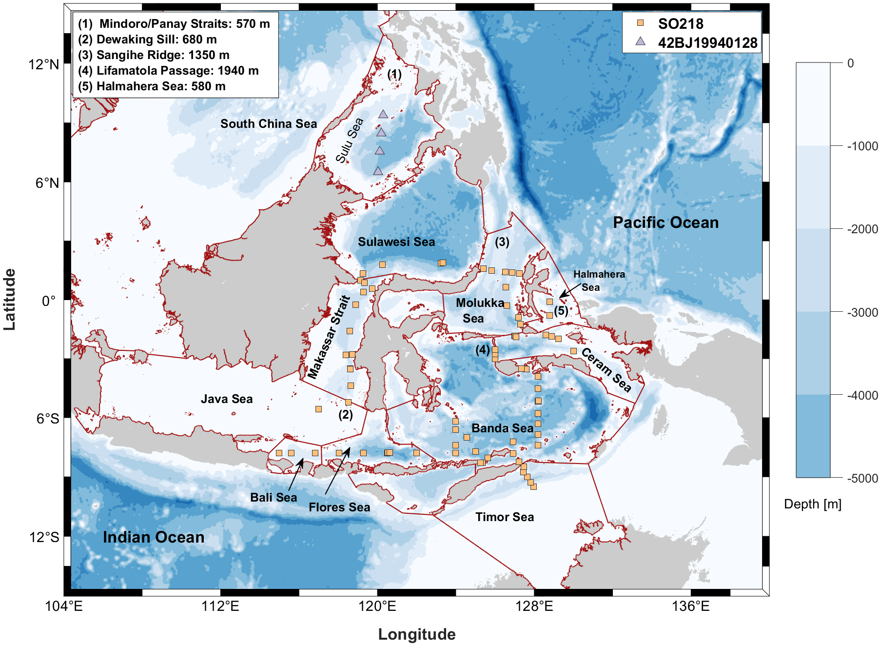
Station map of the selected regions. The dark red solid lines represent the defined sea boundaries [Flanders Marine Institute (2018)]. The numbers on the map indicate the main water exchange channels and their sill depths.
Table 1
| Cruise ID | Year | Area | Sources |
|---|---|---|---|
| SO218 | 2011 | Sulu Sea | (Huang and Tanhua, 2017) |
| 42BJ19940128 | 1994 | Sulawesi Sea, Makassar Strait, Java Sea, Flores Sea, Bali Sea, Molukka Sea, Halmahera Sea, Ceram Sea, Banda Sea, Timor Sea | (Ilahude and Gordon, 2014) |
Information of available source data used in this study.
2.2 Tracer-based age estimates of water
Before describing the OURs, the age of the seawater must be determined. In the ocean, transient tracers such as the CFCs and SF6 can be used as a “clock” to quantify ventilation and transport timescales of water (Fine, 2011; Lu et al., 2014; Stöven et al., 2015). Because CFC observations were conducted in the study regions, transient tracer CFCs were used to estimate the ventilation age of water using the transit-time distribution (TTD) method (Waugh et al., 2003), as will be introduced below.
In fact, ocean interior mixing can cause biases in tracer ages (e.g., Beining and Roether, 1996). In the true ocean, the water parcel consists of waters of different ages. A better way to represent water parcel age is to define a probability distribution of ages (i.e. the TTD) (e.g., Waugh et al., 2003). For stationary transport, the ocean interior concentration C(r,ts) of the tracer at sampling location r and sampling year ts can be expressed as follows:
where the variable t is the transit time required for a water parcel to enter ocean interior from the boundary (usually the surface of the source region where it forms), G(r,t)dt is the mass fraction of the water parcel on the surface at time t to t+dt ago, and C0(ts-t) is the tracer concentration of surface water at the year ts-t. For our calculations, the location r was omitted because each sample data point was calculated separately.
In Equation 1, the symbol “G” is used to represent the TTD. Mathematically, G is a Green’s function that solves the tracer advection-diffusion equation and can be employed to propagate tracer concentrations from the surface to the interior of the ocean. Previous studies showed the TTD has a broad and asymmetric shape (e.g., Khatiwala et al., 2001; Haine and Hall, 2002).
But a general three-dimensional (3D) analytic solution is impossible due to oceanic ventilation complexity. However, it might be accessible for certain idealized flows provided that one was aware of the given parameters, such as the one-dimensional (1D) advection diffusion flow. For 1D steady flow, the solution of TTD is an Inverse Gaussian (IG) distribution (Seshadri, 1999) as follows:
where Γ represents the first moment of G(t) (i.e., the mean age) and Δ denotes the second (centered) moment of G(t) (i.e. the width of the TTD) with given time t. Here, the Δ/Γ ratio indicates the ratio of the advective and diffusivity share in the water parcel. It can be constrained using tracer couples with different input histories. Because only the CFC-12 data could be used independently in this study, we applied an empirical unit ratio of one for water dating. This is appropriate for most upper ocean interior (Waugh et al., 2004).
However, the IG-TTD is a simple approximation for the flows and cannot fully represent the realistic transport in the ocean (Khatiwala et al., 2012). As we only use single transient tracer CFC-12 for this study, other TTDs with more flexible forms like the bimodal two IG-TTDs (Waugh et al., 2003) cannot be used. However, if we focus on the mesopelagic zone in the SEAS, the assumption of 1D advection-diffusion (i.e. the IG form of TTD) might be valid since these waters mainly originate from the adjacent Pacific for the western and eastern pathways of ITF, respectively (Gordon et al., 2003).
2.3 Oxygen utilization rate estimation
Why do we choose oxygen? This is because of the possibility of easily separating the preformed component from the remineralized component. To study the effect of aerobic remineralization on the internal distribution of oxygen in the ocean, we estimated the remineralization component, that is, the change in O2 that occurred when a water parcel was last in contact with the atmosphere. The oxygen concentration is typically close to its saturation concentration at the ocean surface. The equilibrium concentration is assumed to be equal to the preformed oxygen concentration (i.e., Equation 3):
This is available for most oceanic regions because the air-sea equilibration of oxygen is relatively fast compared to the perturbation of disequilibrium. Thus, the commonly used concept of apparent oxygen utilization (AOU) is used to quantify the oxygen utilization resulting from the aerobic remineralization of organic matter. Here (i.e., Equation 4), the AOU is defined as the difference between the actual and equilibrium oxygen concentrations expected from the salinity and temperature of the water.
In a true ocean, directly quantifying the actual OUR is difficult since the respiration rates are very low. One approximate method is to determine OUR by dividing the AOU by the seawater age or the gradient of AOU and age (Karstensen et al., 2008), see Equation 5. Notably, it is the apparent oxygen utilization rate, which is an integrated measure of oxygen consumption by the respiration of marine organisms and/or remineralization of organic matter.
Here, the Γ represents the derived water mean age based on Equations 1 and 2. Care must be taken that the OUR in Equation 5 is a path-integral. However, it cannot be appropriate for providing the measure of the local in-situ OUR. One alternative approach takes OUR as the ratio AOU/age (or the slope of the AOU vs. age regression) to obtain a more local measure of respiration rate (Sonnerup et al., 2013, 2015). But it demands a larger quantity of data and presumes that the isopycnal mean age and AOU fields are parallel-oriented (Sonnerup et al., 2013, 2015).
It is worth noting that the path-integrated OUR is anticipated to be higher than the in-situ OUR. This is because the isopycnals slope downward from the base of the mixed layer, where the oxygen consumption rates are typically higher, towards the ocean interior (Sonnerup et al., 1999). For better comprehension, we will perform a simple estimation demonstration here. For instance, consider a water parcel. It remains at shallow depths for 5 years, where the in-situ OUR is 10 μmol kg-1 yr-1. Subsequently, it spends 15 years at greater depths (i.e., sampling depth), where the in-situ OUR is merely 2 μmol kg-1 yr-1. When this water parcel is sampled at the greater sampling depth, it would have accumulated an AOU of 80 μmol kg-1 (10×5 + 2×15). Consequently, the path-integral OUR is calculated as 80/(5 + 15)=4 μmol kg-1 yr-1, which is twice the in-situ OUR at the sampling depth, namely 2 μmol kg-1 yr-1.
Despite the lack of sufficient data for calculating the gradients of AOU and age, we still employ the aforementioned path-integral method to estimate OUR. The advantage of the approach is that less data are required and we can calculate the OUR for each sample, which is suitable for the overall study of larger-scale regions and can provide spatial trends in the depth-integrated OURs (Sonnerup et al., 2013).
2.4 Arrhenius equation
In this study, we try to explore the potential relationship between temperature and the OUR. This work was motivated by the works of Brewer and Peltzer (2017). The Arrhenius and Eyring equations used by us are fundamental models describing temperature-dependent reaction kinetics, yet they stem from distinct theoretical frameworks. Here, we focus on the Arrhenius equation. For the section on the Eyring equation, please refer to the Supplementary Material. A familiar form of the Arrhenius equation is as follows:
Equation 6 empirically relates the rate constant k to the activation energy (Ea) and temperature (T), where R is the universal gas constant (8.314 J mol-1 K-1) and A is the pre-exponential factor. By introducing the OUR data, we obtained a linear relationship between the natural logarithm of the rate, ln(OUR), and the inverse of the absolute temperature, 1/T, with the slope –Ea/R. Thus, the Ea can be obtained by multiplying the slope by R.
3 Observed data used and derived results
Considering that this study mainly focuses on biochemical reaction kinetics, specifically, the temperature sensitivity of oxygen consumption reactions, various studies over the past few decades have examined the overall oceanographic properties of the sea area (Fine, 1985; Gordon, 1986, 2005; Gordon and Fine, 1996; Gordon et al., 2003; Sprintall et al., 2014, 2009). Therefore, this study will not delve into details on the hydrological properties. Here, we briefly present the general results of the tracers and the derived variables, with a focus on the derived results of the temperature-dependent OURs.
It must be noted that in this study, we used the data which is the scattered bottle data rather than the continuous CTD profile data. Hence, the spatial resolution is insufficient for us to generate gridded section data. As an alternative approach, regional average profiles were depicted for each region, and subsequently, they could be compared to identify the differences between basins. The potential temperature, density, salinity, oxygen, and CFC-derived mean age profiles are presented for the 11 regions (Figures 2, 3).
Figure 2
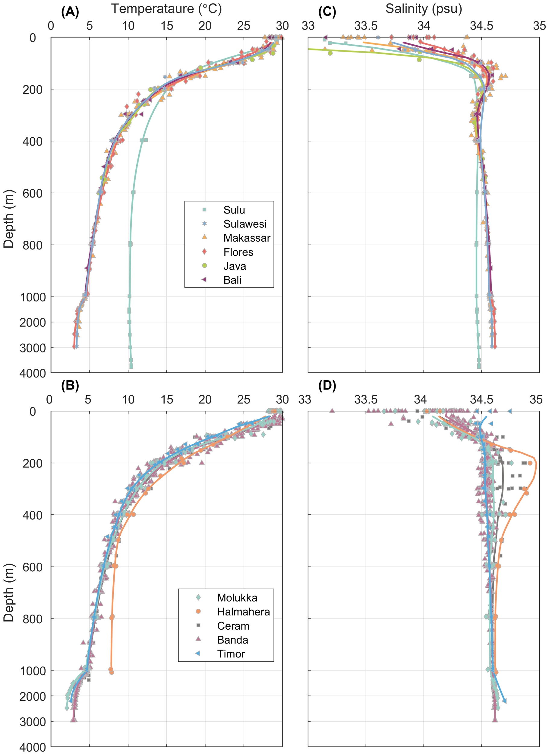
Vertical profiles of (A, B) temperature (°C), (C, D) salinity (psu) for the given regions. The color dots represent the scattered data for all stations. The solid lines represent the mean profiles of the given parameters in each region as defined in Figure 1. Each subplot is divided into two parts with different y axis scale, the upper 1000 m is zoomed in for a better viewing of the characteristics.
Figure 3
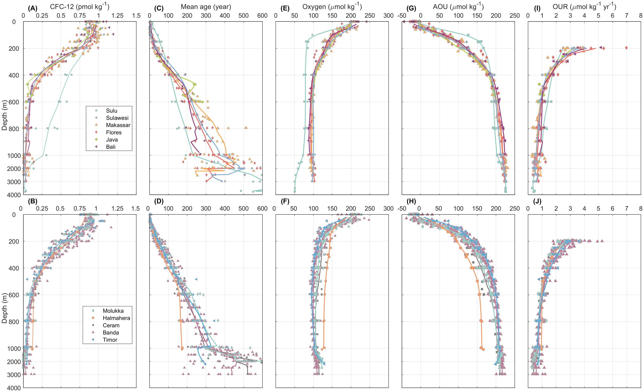
Vertical profiles of (A, B) CFC-12 (pmol kg-1), (C, D) mean age (year), (E, F) oxygen (μmol kg-1), (G, H) AOU (μmol kg-1), and (I, J) OUR (μmol kg-1 yr-1) for the given regions. The color dots represent the scattered data for all stations. The solid lines represent the mean profiles of the given parameters in each region as defined in Figure 1. Each subplot is divided into two parts with different y axis scale, the upper 1000 m is zoomed in for a better viewing of the characteristics. OUR results only show the data below 200 m.
3.1 Hydrology distributions
In terms of temperature, no particularly significant difference was observed among the basins. The temperature at a depth of 1000 m in most areas remained stable at approximately 4–5°C. However, exceptions existed in the Sulu and Halmahera Seas, where distinct temperature variations could be observed compared to the surrounding waters. In the Sulu Sea, the temperature was significantly higher than that of the adjacent Sulawesi Sea below a depth of ~200 m and stayed around 10°C at a depth of 1000 m. A similar situation was also found in the Halmahera Sea, where the temperature was higher than that of the neighboring waters at a depth of approximately 500 m and was 7.7°C at 1000 m depth. Clearly, the water bodies in these two areas were regulated by the sill depth.
The maximum salinity (Smax) of 34.75 for the North Pacific Subtropical Water (NPSW) could be observed at a depth of 150 m in the Makassar Strait. This Smax signal could still be detected in the Flores Sea, though its intensity was not as strong. The Sulu Sea and Sulawesi Seas could also identify the Smax signal. The salinity minimum (Smin) of the North Pacific Intermediate Water (NPIW) was clearly observed in the Makassar Strait at σθ=26.5 with a salinity of approximately 34.45. This core of the Smin could also be found downstream in the Flores, Java, Bali Seas and the Banda Sea, with a diminished intensity of the Smin. There was no notable Smin in the Sulu Sea.
For the eastern path, the Halmahera Sea sill depth is 580 m (Figure 1). A distinct Smax could be found at ~250 m in the Halmahera Sea and in the Ceram Sea. This salty water should be derived from the adject South Pacific (Gordon and Fine, 1996; Ilahude and Gordon, 1996) and could be characterized by a Smax of ~34.9 located on σθ of 26.0 and extended to the depth range from about 200–600 m in the Molukka, Ceram and Banda Seas. For the depth between 600–1000 m, a Smin core could be found in the Molukka and Ceram Seas. This Smin core was attributed to the signal of Antarctic Intermediate Water (AAIW) and it attenuates in the Ceram Sea and cannot be found in the Banda Sea (Gordon et al., 2003).
3.2 CFC-12, mean age and OUR distributions
Figures 3A, B shows the vertical profiles of CFC-12 for all basins. As shown in Figures 3A, B, detectable concentrations of CFC-12 were found throughout the water column from the surface to the depth of 1000 m where the CFC-12 concentrations were lower than 0.1 pmol kg-1. Below the surface layer, the CFC-12 decreased monotonically, although there were some differences among the basins. The Sulu Sea revealed a very different shape of profile compared to the adjacent seas where high concentrations of CFC-12 could be found below the depth of 400 m. Such the value of CFC-12 concentrations below the surface layer was the highest all around the basins and revealed a special ventilation source i.e., from the South China Sea through the Mindanao/Panay Starits (Huang and Tanhua, 2017; Gordon et al., 2011). Similar tendencies could also be observed in the Halmahera Sea where the CFC-12 concentrations were higher than those in the Ceram and Molukka Seas below a depth of ~600 m, but it was not as noticeable as those in the Sulu Sea.
The mean ages derived from CFC-12 data were also presented in Figures 3C, D. Generally, the distribution of mean ages exhibited reverse tendencies in relation to the concentrations of CFC-12. For the upper layer above 400 m, there was no significant CFC-derived mean age gradient from northern Makassar to the Banda Sea. That is, the mesopelagic water of the Banda Sea was mainly ventilated by the flow from the Flores Sea (Waworuntu et al., 2000). The mean age in the Hamehara Sea was the youngest below sill depth (580 m) compared with that in the Mulukka, Ceram, and Banda Seas. A similar trend of a relatively younger mean age was also detected in the Sulu Sea compared to the adjacent Sulawesi Sea. Contrary to the feature of concentration distribution, the mean age distribution tended to disperse with increasing depth, mainly due to the higher uncertainty propagation from the lower concentration.
Figures 3I, J presented the vertical distribution of path-integrated OUR for the 11 regions. At a depth of approximately 200 m, the values of OUR exhibited considerable fluctuations, with the maximum value approaching 7 μmol kg-1 yr-1 and the most of OUR ranging from 2 to 6 μmol kg-1 yr-1. Subsequently, the OUR decline in an approximately exponential manner with depth. At a depth of 1000 m, OUR decreased to approximately 1 μmol kg-1 yr-1. The exception occurs in the Sulu Sea and the Hamaheera Sea, where OUR remain marginally higher than in adjacent waters at depths below 600 m. This disparity is likely the consequence of a combination of water mass transport, oxygen consumption, temperature, and other processes. We will employ the fitting results of the Arrhenius equation and subsequent discussions to explain this.
3.3 Results derived from Arrhenius equation
3.3.1 Integration result of the entire region
First, we considered the general distribution of all regions. Figure 4 shows scatter plots of all available OUR versus the reciprocal of temperature for the entire studied region. We focused on the mesopelagic zone (the red dots in Figure 4), where the AOU is mainly influenced by the microbial degradation of organic matter, which consumes oxygen, thereby eliminating oxygen interference from photosynthesis in the euphotic zone.
Figure 4
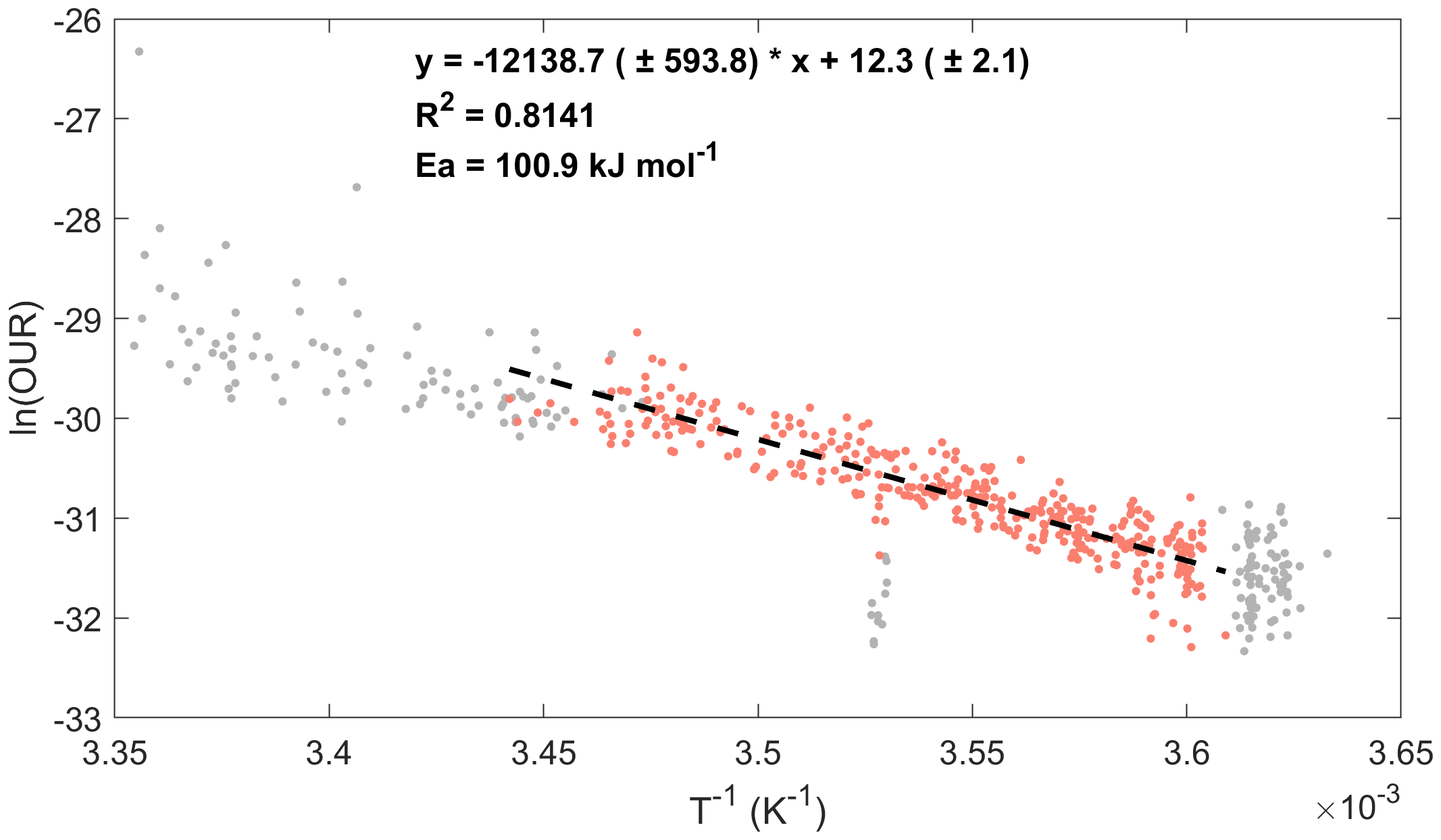
All qualified datasets are plotted as an Arrhenius function, as indicated in the text. The Arrhenius activation energy (Ea) of 100.9 kJ mol-1 was calculated from this data ensemble. The red dots represent the data used for fitting within the depth ranging from 200 to 1000 m, while the grey dots represent the remaining data points. And the black dashed line represents the fitting curve.
Overall, a significant linear correlation was observed between the logarithm of the OUR and the reciprocal temperature, with a coefficient of determination (R2) of 0.81. Thus, the results showed a significant linear correlation between the OUR and temperature, which was characterized by the classical Arrhenius equation. Without accounting for regional differences, we obtained an average Ea = 100.9 kJ mol-1 for the entire studied region. This overall mean was consistent with previous estimates for the low-latitude Pacific Ocean (Brewer and Peltzer, 2017) and South China Sea (Huang et al., 2024). We believe that this number is the overall mean value for the region. The activation energies derived from the strong correlation between temperature and the OUR reflected the apparent average state, or baseline, over the entire ocean.
3.3.2 Regional result of the basins
Although the overall results appeared to match well, we expected to observe differences in the correlation between temperature and OUR in different regions of Southeast Asian waters. Using the same process described in Section 3.2, we fit the data of the 11 sea areas separately. The results are summarized in Table 2 and Figure 5, which show graphical representations of the data in the requisite format for calculating the Arrhenius activation energy for each investigated region.
Table 2
| Region | Ea (kJ mol-1) | R2 | Temperature (°C) | Q2 | Q10 | n |
|---|---|---|---|---|---|---|
| Sulu Sea | 139.2 | 0.67 | 10.16–14.27 | 1.52 | 8.20 | 12 |
| Sulawesi Sea | 125.2 | 0.98 | 4.36–14.72 | 1.46 | 6.63 | 10 |
| Makassar Strait | 123.1 | 0.81 | 4.35–15.38 | 1.45 | 6.43 | 51 |
| Java Sea | 126.1 | 0.91 | 6.24–14.55 | 1.46 | 6.72 | 9 |
| Flores Sea | 133 | 0.95 | 4.45–14.88 | 1.49 | 7.47 | 27 |
| Bali Sea | 111.9 | 0.95 | 4.40–14.68 | 1.40 | 5.43 | 19 |
| Molukka Sea | 101.9 | 0.87 | 4.36–16.11 | 1.36 | 4.66 | 38 |
| Halmahera Sea | 82.6 | 0.98 | 7.75–17.22 | 1.28 | 3.48 | 12 |
| Ceram Sea | 77 | 0.91 | 4.67–15.54 | 1.26 | 3.20 | 38 |
| Banda Sea | 97.9 | 0.86 | 3.93–17.38 | 1.34 | 4.39 | 125 |
| Timor Sea | 109.1 | 0.90 | 4.65–14.33 | 1.39 | 5.20 | 30 |
Properties of the thermodynamic parameters derived from Arrhenius equation. The data used for the fitting process comprised a range of 200–1000 m.
Figure 5
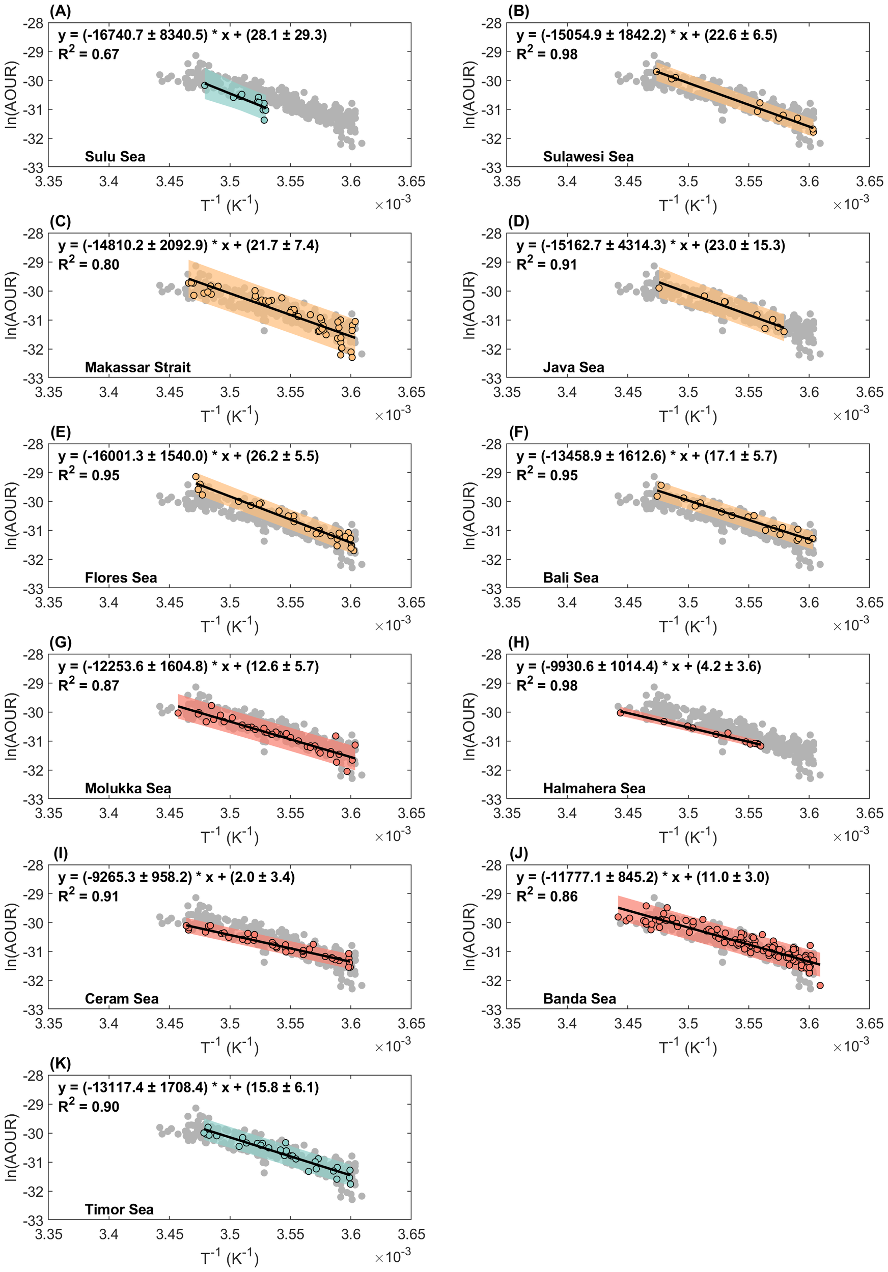
Arrhenius activation energy fitting plots for the (A) Sulu Sea, (B) Sulawesi Sea, (C) Makassar Strait, (D) Java Sea, (E) Flores Sea, (F) Bali Sea, (G) Molukka Sea, (H) Halmahera Sea, (I) Ceram Sea, (J) Banda Sea and (K) Timor Sea. The color dots represent the data used for fitting within the depth ranging from 200 to 1000 m, while the grey dots represent the remaining data points. The black line represents the fitting curve, whereas the color shadow represents the prediction interval within a 95% confidential level.
The Ea of Sulu Sea were the For the Sulu Sea, we refined the data and recalculated all the energies to better understand the regional differences. This is because the original data of the Sulu Sea was deduced by Huang et al. (2024) from a roughly apparent rate constant based on the quasi-first order assumption. highest of all basins, at 139.2 kJ mol-1.The most notable difference in the Sulu Sea was its linear correlation, and the R2 was 0.67 (Figure 5A), which was the lowest among all results in the basins. This may be due to constraints at a depth of approximately 600 m, which is discussed in Section 4.
The results for Sulawesi Sea, Makassar Strait and Java Sea were close, with Ea of 125.2, 123.1 and 126.1 kJ mol-1, respectively. The Flores Sea connects to the Makassar Strait via the Dewakang Sill (approximately 680 m). The fitting results also showed an Ea value of 133 kJ mol-1, which were the highest around the western path of the ITF but smaller than that of the Sulu Sea. This could be due to topographic barriers, as discussed in Section 4. The Bali Sea, one of the ITF outlets through the Lombok Strait, has an Ea of 111.9 kJ mol-1, which was the smallest around the west path of the ITF but was within the same magnitude as compared to the east path region of ITF.
The northern and northwestern sides of the Maluku Sea are connected to the Pacific Ocean and Sulawesi Sea, respectively, whereas the southern side is connected to the Banda and Ceram Seas through a series of channels. Its results were lower than those of the adject Sulawesi Sea, revealing a potentially different apparent oxygen consumption pattern. The Halmahera Sea is divided by a submarine ridge that increases to a depth of approximately 700 m, forming a sill that acts as an entrance portal for South Pacific high-salinity subtropical water. Thus, the relationship between temperature and the OUR significantly differed from that of its neighboring eastern and northern basins, as described previously. The relatively small results may reflect differences in oxygen consumption owing to their unique water sources.
The Ceram Sea, similar to the Halmahera Sea to the north, has the lowest fitting value with an Ea of 77.0 kJ mol-1. The number of data points (n = 265) in the Banda Sea was the greatest for all the basins in the research areas. The relatively low value of the Banda Sea suggests that it should be a potential water source that supplies the “fresh” water with liable organic matter. This indicates that the water may have been influenced by southern sources from the South Pacific Ocean. However, the Timor Sea is outside the Indonesian seas and is part of the Indian Ocean. It connects to the northern Banda Sea, where the ITF flows into the Timor Sea and Indian Ocean. The fitting Ea (109.1 kJ mol-1) of the Timor Sea were at a relatively moderate level within the 11 sea regions in this study. This appears to be a combination of water from the North and South Pacific sources.
4 Discussions
Based on the overall distribution characteristics, it was evident that the influence of temperature on the OURs was consistently notable. The average Ea in the entire SEAS region was 100.9 kJ mol-1 (Figure 4), consistent with previous studies on the temperature correlation of OURs (Brewer and Peltzer, 2017; Huang et al., 2024; Wang C. et al., 2021; Wang W. et al., 2021). However, differences remained between the various basins within the SEAS when considering specific regions.
First, we will discuss the derived temperature sensitivity of OUR to temperature, as this is a key issue in this study. Subsequently, the potential spatial distributions around the basins and their impacts on the derived Ea will be explored.
4.1 Temperature sensitivity of estimated OUR
The Ea derived from the Arrhenius equation provides an analysis of the kinetic impact of temperature on OUR from the perspective of energy threshold (discussed previously). To further correlate with the temperature effect in observational data or models, the Q10 is introduced here, which can be used to describe the overall temperature response of complex biological systems (Davidson and Janssens, 2006; Bendtsen et al., 2015). At the same time, it offers an intuitive multiple relationship (dimensionless), facilitating cross-ecosystem comparisons and quantitative assessment of the impact of ocean warming under climate change scenarios on the reduction of dissolved oxygen. It is important to note that the actual Q10 value is not constant. It decreases non-linearly with increasing temperature (underestimating at low temperatures and overestimating at high temperatures) (Lloyd and Taylor, 1994). Therefore, it is only effective within a certain temperature interval, and needs to be recalibrated when the temperature interval is changed.
The calculation results are presented in Tables 2 and 3, Figure 6. The calculated activation energies (Ea) ranged from 77.0 kJ mol−1 (Q10 = 3.2) in the Halmahera Sea to 139.2 kJ mol-1 (Q10 = 8.2) in the Sulu Sea, which was attributed to the unique hydrology causing non-steady-state conditions. Regionally, Q10 clustered into western (6.4–7.5) and eastern (3.2–4.7) pathways, reflecting distinct microbial community adaptations.
Table 3
| Depth range | 200–600 m | 600–1000 m | ||||||||
|---|---|---|---|---|---|---|---|---|---|---|
| Regions | Ea | R2 | Temperature | Q10 | n | Ea | R2 | Temperature | Q10 | n |
| (kJ mol-1) | (°C) | (kJ mol-1) | (°C) | |||||||
| Sulu Sea | 93.5 | 0.83 | 14.27–10.62 | 4.11 | 7 | 513.6 | 0.46 | 10.72–10.16 | 2349.67 | 8 |
| Sulawesi Sea | 122.3 | 0.97 | 14.72–6.30 | 6.35 | 7 | 147.4 | 0.83 | 6.57–4.36 | 9.27 | 5 |
| Makassar Strait | 107.5 | 0.85 | 15.38–6.22 | 5.08 | 37 | 130.1 | 0.16 | 6.72–4.35 | 7.15 | 23 |
| Bali Sea | 112.4 | 0.93 | 14.68–6.34 | 5.47 | 14 | 132.9 | 0.49 | 6.34–4.40 | 7.45 | 6 |
| Flores Sea | 131 | 0.94 | 14.88–6.60 | 7.24 | 17 | 117.6 | 0.48 | 6.86–4.45 | 5.92 | 14 |
| Molukka Sea | 101.3 | 0.92 | 16.11–6.60 | 4.62 | 30 | 78.8 | 0.15 | 7.24–4.36 | 3.29 | 13 |
| Halmahera Sea | 81 | 0.97 | 17.22–8.13 | 3.40 | 9 | 53.3 | 0.37 | 8.44–7.75 | 2.24 | 5 |
| Ceram Sea | 73.1 | 0.86 | 15.54–7.05 | 3.02 | 28 | 93 | 0.55 | 7.73–4.67 | 4.08 | 14 |
| Banda Sea | 90.5 | 0.83 | 17.38–6.38 | 3.93 | 81 | 118.5 | 0.46 | 7.58–3.93 | 6.00 | 65 |
| Timor Sea | 98.6 | 0.85 | 14.33–6.72 | 4.44 | 24 | 146.3 | 0.57 | 6.93–4.65 | 9.13 | 9 |
| Java Sea* | 126.1 | 0.91 | 14.55–6.24 | 6.72 | 9 | 6.24 | 1 | |||
Derived activation energy (Ea) and temperature coefficient (Q10) for the depth range of 200–600 m and 600–1000 m, respectively. ‘R2’ represents the coefficient of determination between ln(OUR) and the reciprocal of absolute temperature (K-1).
*Insufficient data for fitting to the Java Sea within 600–1000 m.
Figure 6
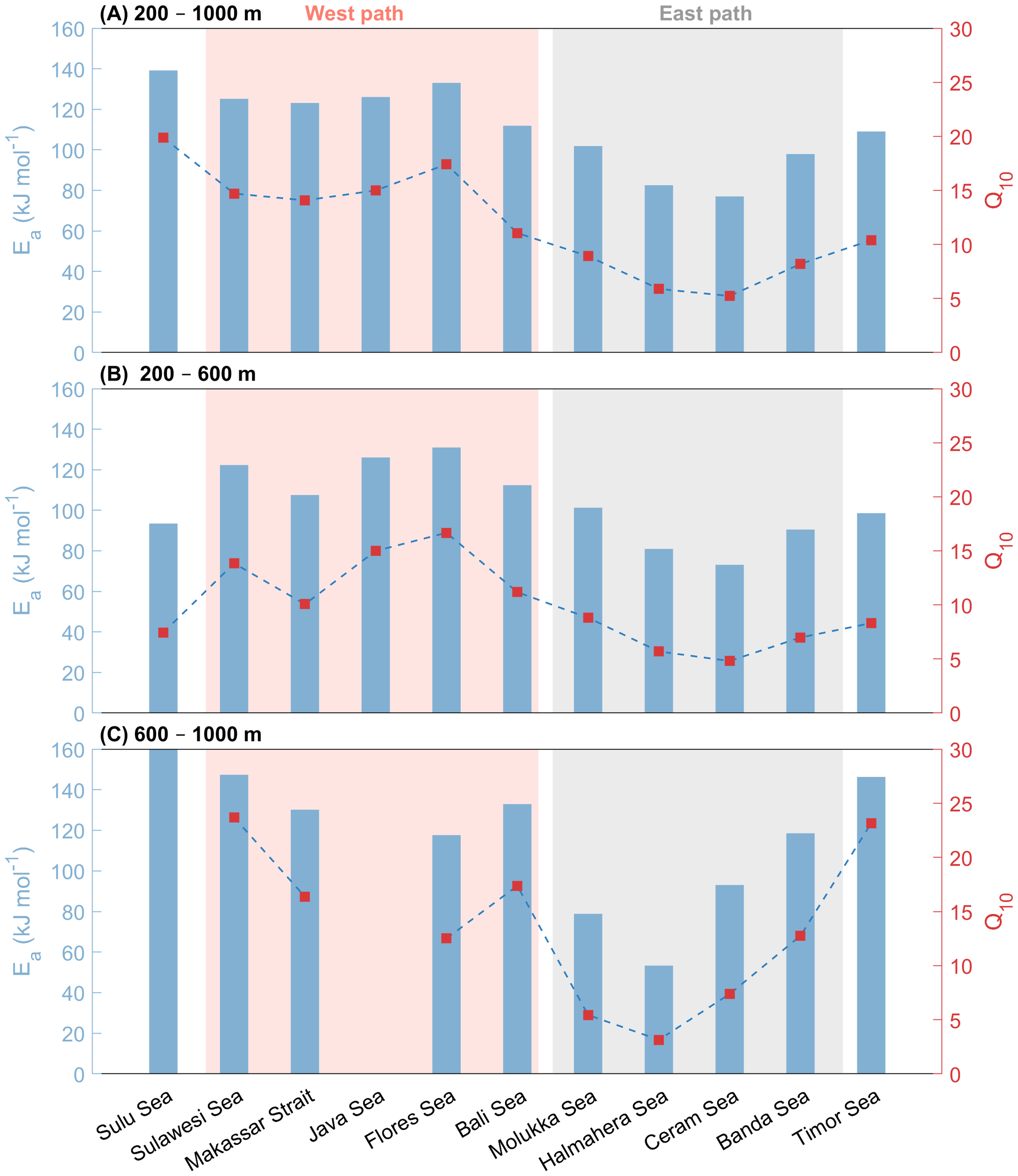
Bar chart of the derived activation energy Ea together with the dash-dot line of derived Q10 for all the 11 regions within the depth range of (A) 200–1000 m, (B) 200–600 m, and (C) 600–1000 m, respectively. The light pink and grey shades represent the west and east paths of the ITF, respectively. Note that the Ea of the Sulu Sea (513.6 kJ mol-1) is beyond the y-axis limit of the plot.
These values are in alignment with incubation studies: Bendtsen et al. (2015) reported Q10 of 1.9–2.1 for particulate organic carbon (POC) and 5.1–6.8 for total organic carbon, while sediment/soil studies show analogous temperature dependencies (Q10 of 1.8–4.4) (Thamdrup and Fleischer, 1998; Craine et al., 2010). This consistency across marine, terrestrial, and benthic systems underlines the temperature sensitivity of organic matter degradation by microorganisms within the natural temperature range of marine environments in accordance with the general reaction kinetics principles (e.g., the Arrhenius equation). Notably, lower baseline temperatures in our study (~10°C vs. soil studies at 20°C) may slightly inflate Q10 estimates.
Thus, similar to Q10, we also calculated Q2, i.e., a 2°C warming scenario, which amplified OUR by 30.7% (western path, Ea=89.8 kJ mol-1) and 45.9% (eastern path, Ea=126.8 kJ mol-1), demonstrating significant thermal sensitivity. Such effects challenge traditional biogeochemical models that underestimate temperature-responsive feedbacks. Marine systems exhibit comparable microbial thermal adaptations to those in soils/sediments, where recalcitrant organic matter enhances respiration sensitivity (Davidson and Janssens, 2006; Fierer et al., 2005).
While physical oceanographic changes dominate climate discussions, these results emphasize microbial temperature sensitivity as a critical amplifier of carbon cycling under warming. Given the projected oceanic warming, we propose adopting Q2 (2°C warming intervals) rather than Q10 for climate predictions of biogeochemical feedbacks in dynamic ocean systems.
4.2 Regional differences of Ea between the basins
Our findings revealed significant disparities in the Ea between the eastern and western paths of the ITF (Figure 6). This observation was particularly intriguing, suggesting a substantial intrinsic correlation between temperature and OUR. The impact of temperature on oxidation of organic matter in distinct sea basins is undeniably profound and warrants careful consideration. Notably, the data indicated that the mean Ea for the western path was 126.8 ± 4.3 kJ mol-1, whereas for the eastern path it was 89.8 ± 11.9 kJ mol-1. We attributed this discrepancy to variations in ITF sources and pathways (Gordon, 2005; Gordon and Fine, 1996).
The AOU and its variational gradient were significantly higher along the western path than the eastern one (Figures 3G, H). Two main sources of the ITF exist: North Pacific mesopelagic water flowing through the Sulawesi and Maluku seas and high-salt, oxygen-rich (low-AOU) South Pacific source water flowing through the Halmahera Sea, which has also been observed in the Maluku, Seram, and Banda seas (Gordon, 2005; Gordon and Fine, 1996; Gordon et al., 2003). In the ocean interior, microorganisms preferentially consume easily decomposable organic matter, thereby generating more chromophoric dissolved organic matter (CDOM) and fluorescent dissolved organic matter (FDOM) that are resistant to biological degradation (Yamashita and Tanoue, 2008). Previous studies have confirmed that there is a significant positive linear relationship between AOU and CDOM or FDOM in the mesopelagic of the Pacific Ocean, although the slopes vary in different regions due to water mass mixing (Nelson et al., 2010; Yamashita and Tanoue, 2008). The North Pacific mesopelagic water, which serves as the source of the western path, accumulates FDOM produced in situ due to limited ventilation. At the same time, it also carries terrestrial FDOM from the shelf sediments of the Sea of Okhotsk, which will form complexes with iron and then are transported conservatively to the western part of the subtropical North Pacific Ocean and over long distances (Yamashita et al., 2020, 2021). Their resistance to degradation is further enhanced (Yamashita et al., 2020). In contrast, the FDOM in the mesopelagic of the South Pacific is mostly produced in situ depending on oxygen consumption. The negative deviation of the AOU-FDOM relationship found in AAIW also indicates that the preformed FDOM content is low and is subject to photo degradation (Yamashita et al., 2007; Yamashita and Tanoue, 2008). According to the Arrhenius equation, the bioavailability of organic matter as a substrate for aerobic respiration can reflect the reaction’s Ea. Therefore, within the visible temperature range (4 – 14°C), the fitted slopes of the two paths differ, with the western path having a greater slope than the eastern one. In other words, the OUR on the west side was more temperature-sensitive than that on the east side.
Here, we did not discuss the typical depth profile of the OUR but provided a method to identify the sources of different water masses. However, notably, the OUR and path method were used in this study. This approach calculates the average OUR (Sonnerup et al., 2013) of water moving from the source area to the sampling point in the ocean interior. The instantaneous rate (i.e., the oxygen gradient and age of the given isopycnal) may better characterize the OUR in the study area. However, this will require further intensive observations of the data and more accurate dating in the future.
4.3 Causes of typical Arrhenius relationship deviations
4.3.1 General view of the temperature-dependent OUR
The molecular structure of organic matter and environmental temperature are important factors regulating the temperature sensitivity of aerobic respiration processes, also known as intrinsic temperature sensitivity (Knorr et al., 2005; Davidson and Janssens, 2006). Theoretically, for organic matter with higher stability, the decomposition process under low-temperature conditions exhibits higher temperature sensitivity (with a higher Ea value) (Davidson and Janssens, 2006). However, environmental constraints such as physical mixing (Huang et al., 2024; Brewer and Peltzer, 2017), substrate availability (Maske et al., 2017), and microbial community composition (Letscher et al., 2015; Nelson and Carlson, 2012; Zogg et al., 1997) can mask the true impact of temperature, thereby causing the (apparent) temperature sensitivity observed to be lower than the expected temperature sensitivity.
From the perspective of the entire mesopelagic zone of SEAS, the linear relationship between ln(OUR) and 1/T (K−1) is significant. The relationship depicted in Figure 5 explains 67 – 98% of the variation in OUR as a function of temperature in the form of the Arrhenius equation for SEAS throughout the depth range of 200–1000 m. After the division at 600 m, the OUR in the 200–600 m still maintained a good correlation with temperature. Moreover, the temperature and organic matter can account for the observed sensitivity and could be explained over than 80% of the variation (Table 3). In most basins, the Ea in the 200–600 m is close to that of the entire mesopelagic zone, indicating that the OUR in the 200–600 m is also regulated by temperature, and its contribution to the temperature sensitivity of the entire mesopelagic zone has also been found. Nevertheless, it appears that OURs are significantly and systematically underestimated at low temperatures below ~600 m depth. Table 3 summarizes the outputs of the results for different depth ranges.
4.3.2 Oceanic transport modulation of the OUR-temperature correlation
During the vertical downward transport of organic matter, microbial remineralization will preferentially utilize the most labile components, such as carbohydrates and dissolved combined neutral sugars, and gradually accumulate recalcitrant components (Hansell et al., 2009; Hansell, 2013). Coupled with the decrease in temperature, it further enhances the intrinsic temperature sensitivity of OUR in the deeper layers of the mesopelagic zone. For instance, Ea in Sulawesi Sea increased from 122.3 kJ mol-1 at 200–600 m to 147.4 kJ mol-1 at 600–1000 m. However, the relationship between OUR and temperature at depths of 600–1000 m in most basins deviates from the classical Arrhenius equation featuring a lower R2 compared to that in the upper 200–600 m, and these regions are subject to varying degrees of environmental constraints.
Hydrological transport is one of the influencing factors. The most obvious manifestation is Sulu Sea, where the nearly uniform temperature and salinity at depths below 600 m indicate good mixing (Figure 3). The rapid ventilation results in a decoupling between the OUR and the water aging rate. Similar patterns were noted in the Mediterranean Sea, Red Sea, and Sea of Japan, where rapid influxes under terrain-driven gradients disrupt steady-state oxygen consumption (Brewer and Peltzer, 2017; Huang et al., 2024). Such vigorous mixing processes might obscure the original temperature sensitivity observed at 600–1000 m.
The Flores Sea stands in contrast with the Sulu Sea. Its Dewakang Sill (680 m) lacks a steep OUR-temperature curve, instead resembling the Banda Sea’s profile. Upper-layer (200–600 m) Ea was 131 kJ mol-1, aligning with the Banda Sea’s deeper value (118.5 kJ mol−1) (Figures 3G, H). This reflects ventilation pathways: Flores Sea deep water originates from Banda Sea overflow via the Lifamatola Passage, while Makassar Strait water is supplied by Sangihe Ridge overflow (Gordon et al., 2003). No stratification discontinuity exists across the Dewakang Sill, as shown by AOU profiles (Figure 3G).
Meanwhile, the hydrological transport process can alter the regional oxygen consumption pattern by adjusting three key factors related to organic matter transformation: temperature, supply of labile substrate, and oxygen (Wang C. et al., 2021). The Halmahera Sea shows no sharp OUR-temperature “turning point” like the Sulu Sea. Its lower AOU and cooler deep-water temperatures reduced temperature sensitivity compared to the Sulu Sea, where elevated temperatures enhance microbial oxygen consumption of refractory organic matter. This mismatch between microbial enzyme activity and temperature creates high Arrhenius-derived sensitivity in the Halmahera Sea, despite similar sill depths.
4.3.3 The role of substrate limitation and microbial communities
Substrate availability is another non-negligible factor. Maske et al. (2017) investigated the differences in metabolic responses of coastal microbial communities to temperature changes under substrate limitation and non-limitation conditions. Their results showed that in substrate-limited environments, microbial communities maintained a constant ratio between specific respiration rate and specific growth rates, enabling carbon growth efficiency to be independent of temperature. In this case, the specific respiration rate was mainly determined by the growth rate, and the temperature sensitivity of microbial respiration might not represent the overall response of OUR to temperature changes. However, although the water masses of the ITF originating from the tropical western Pacific are typically oligotrophic (Chen et al., 2021), the strong vertical mixing effects induced by the convergence of steep topography, narrow straits, and dynamic circulation supply the SEAS with abundant nutrients (Xie et al., 2024). Studies have shown that the vertical flux of NO3− is as high as 6.9 ± 7.9 mmol m⁻² d−1, which is nearly two orders of magnitude higher than the horizontal flux and accounts for approximately 98% of the total nutrient supply (Xie et al., 2024). Significant high chlorophyll-a and net community production were observed at the entrances and exits of the Makassar Strait, southern Sulawesi Sea, the entrance of the Maluku Sea, and the Halmahera Sea (Xie et al., 2024). The substrate availability does not seem to be the primary limiting factor for these basins.
Another hypothesis is that microbial communities influence OUR by regulating the bioavailability of DOC (as well as the respiration rate) (Robinson, 2019). In the ocean, the dynamic changes in the concentration of DOC are mainly controlled by two key oxidation processes: one is the mineralization of DOC to CO2, and the other is the oxidation of POC to release DOC (Seritti et al., 2003). These processes are mainly driven by the intense biological activities of bacteria and protists (Cho and Azam, 1988; Smith et al., 1992). Therefore, the generation mechanism of DOC is largely influenced by the plankton community structure (Carlson and Ducklow, 1995; Hansell and Waterhouse, 1997). There are significant differences in decomposition capabilities among microbial communities at different depths (Letscher et al., 2015), and specific microbial groups have selectivity in their utilization efficiency for different DOC substrates (Nelson and Carlson, 2012; Lønborg et al., 2022), which ultimately manifests in the spatial differences of OUR. Both being tropical seas, the microbial communities in the Red Sea have a relatively weak response to temperature and substrates. However, the Great Barrier Reef near SEAS significantly accelerated the metabolic activities of microorganisms and the hydrolysis efficiency of extracellular enzymes when the temperature increased (+3°C gradient), thereby enhancing the bioavailability of DOC (Lønborg et al., 2022). When different DOC types dominate (such as monosaccharides—Copiotrophs, and cyanobacterial secretions—Oligotrophs), the communities exhibit different metabolic responses (Nelson and Carlson, 2012), which will lead to significant differences in OUR at the same temperature, potentially neutralizing or masking the overall temperature sensitivity. This might also be the reason why the correlation between OUR and temperature at 600–1000 m in SEAS is relatively weak.
Moreover, it may also be related to the active transport mechanism of vertical migration of zooplankton. On the one hand, such large-scale migrations may have a significant impact on the microbial community structure (Breusing et al., 2022); on the other hand, the adaptive adjustments they have made to tolerate the low temperature and low oxygen environment in deep water may have reduced their temperature sensitivity (Cavan et al., 2017). However, more experimental or observational evidence is needed to support this.
4.3.4 Summary
In general, the physiological responses of microorganisms to temperature are much more complex than what Arrhenius parameterization indicates, and they can affect specific metabolic pathways in different ways (Maske et al., 2017). Overall, the basin-specific hydrography, sill-driven circulation, and other environmental conditions modulate the oxygen consumption patterns of SEAS, which makes it necessary to be cautious when extrapolating Arrhenius-based models.
It should be also noted that data quality has a significant impact on the interpretation of results. For the Maluku Sea, the original Ea of 78.8 kJ mol-1 (600–1000 m) with low R2 (0.15) conflicted with expected trends. After excluding discrete data points (Supplementary Figure 1), revised values (Ea = 156.7 kJ mol-1, R2 = 0.71) aligned better with observed organic matter degradation and terrain-constrained ventilation imbalances. Similar adjustments slightly raised the 200–1000 m Ea to 111.2 kJ mol-1 (R2 = 0.93), emphasizing data quality impacts on interpretation. Furthermore, due to the extremely low OUR at the 600–1000 m and the limited temperature variation range, the fitting of the Arrhenius equation is subject to significant uncertainty. This data may not accurately capture the true temperature sensitivity characteristics of the oxygen consumption process at this depth range.
5 Conclusion
Our study demonstrates that in the mesopelagic zone (200–1000 m) of the SEAS, OUR exhibit strong temperature dependence under near-steady-state conditions. The Arrhenius-derived apparent activation energy (Ea) averaged ~100 kJ mol−1 across the entire region, aligning with global oceanic estimates. Notably, striking differences emerged between the western (126.8 ± 4.3 kJ mol-1) and eastern ITF pathways (89.8 ± 11.9 kJ mol-1), likely reflecting contrasting water mass origins—North Pacific-derived vs. South Pacific-sourced—that modulate organic matter lability and ventilation dynamics.
A stratified analysis was conducted on the range of 200–1000 m. The results revealed that the OUR in the upper 200–600 m still exhibited a strong temperature dependence, and the Ea in multiple basins were close to the Ea obtained based on the entire mesopelagic. Deviations from the classical Arrhenius equation were observed at 600–1000 m. These regions were subject to varying degrees of environmental constraints. Physical processes (such as mixing and water mass transport) as well as biological factors (such as substrate availability and microbial community composition) might alter the local oxygen consumption patterns, thereby blurring the regulatory effect of temperature on OUR. It also reminds us that when extrapolating based on the Arrhenius model, the influence of environmental constraints on the OUR must be taken into account. Under a 2°C warming scenario, it is projected that OUR increases of 30.7% (western pathway) and 45.9% (eastern pathway), respectively. Although physical factors have often been discussed in past studies on warming oceans, these results reveal that temperature is also a critical amplifier of biogeochemical feedbacks.
This study has unresolved questions. First, we still need sufficient data to make time-series observations to understand these changes. Second, although the calculation method for the OUR allows us to calculate and compare each sample data point with a single point, the OUR belongs to the mean value of a motion path, which remains affected by the initial equilibrium condition. The gradient method (i.e., the slope of oxygen concentration vs. age within a given isopycnal) might be more appropriate. However, this would require conducting additional observations to obtain more data. At a depth of more than 1000 m, CFC-12 may fall below the limit of detection, causing the result fitting to diverge. Therefore, deep dating data (such as argon-39 and carbon-14) can be obtained to calculate the mean age. Simultaneously, the computational bias due to potential upwelling must also be considered. In the Banda Basin, in particular, we must explore potential ways to separate the effects of physical and biological processes to obtain a purer rate of oxygen consumption. Although culture experiments are possible, they are not complete substitutes for large-sample data in the field.
Statements
Data availability statement
The original contributions presented in the study are included in the article/Supplementary Material. Further inquiries can be directed to the corresponding author. The synthetic dataset, which includes tracer data and derived data required for obtaining the main results of this study, has been deposited on Zenodo at https://zenodo.org/records/14951133. This link contains the derived data used for plotting and the data processing codes.
Author contributions
ZL: Formal Analysis, Methodology, Writing – original draft, Writing – review & editing. PH: Data curation, Supervision, Writing – original draft, Writing – review & editing.
Funding
The author(s) declare financial support was received for the research and/or publication of this article. This work was supported by the National Natural Science Foundation of China (NO. 41906041), Natural Science Foundation of Guangdong Province, China (NO. 2024A1515030185) and the Program for Scientific Research Start-Up funds of Guangdong Ocean University.
Acknowledgments
We gratefully thank the reviewers for their thorough and constructive suggestions.
Conflict of interest
The authors declare that the research was conducted in the absence of any commercial or financial relationships that could be construed as a potential conflict of interest.
Generative AI statement
The author(s) declare that no Generative AI was used in the creation of this manuscript.
Any alternative text (alt text) provided alongside figures in this article has been generated by Frontiers with the support of artificial intelligence and reasonable efforts have been made to ensure accuracy, including review by the authors wherever possible. If you identify any issues, please contact us.
Publisher’s note
All claims expressed in this article are solely those of the authors and do not necessarily represent those of their affiliated organizations, or those of the publisher, the editors and the reviewers. Any product that may be evaluated in this article, or claim that may be made by its manufacturer, is not guaranteed or endorsed by the publisher.
Supplementary material
The Supplementary Material for this article can be found online at: https://www.frontiersin.org/articles/10.3389/fmars.2025.1503255/full#supplementary-material
References
1
Arrhenius S. (1889). Über die Reaktionsgeschwindigkeit bei der Inversion von Rohrzucker durch Säuren. Z. Phys. Chem.4U, 226–248. doi: 10.1515/zpch-1889-0416
2
Beining P. Roether W. (1996). Temporal evolution of CFC 11 and CFC 12 concentrations in the ocean interior. J. Geophys. Res. Oceans101, 16455–16464. doi: 10.1029/96JC00987
3
Bendtsen J. Hilligsøe K. M. Hansen J. L. S. Richardson K. (2015). Analysis of remineralisation, lability, temperature sensitivity and structural composition of organic matter from the upper ocean. Prog. Oceanogr.130, 125–145. doi: 10.1016/j.pocean.2014.10.009
4
Breusing C. Osborn K. J. Girguis P. R. Reese A. T. (2022). Composition and metabolic potential of microbiomes associated with mesopelagic animals from Monterey Canyon. ISME Commun.2, 117. doi: 10.1038/s43705-022-00195-4
5
Brewer P. G. Peltzer E. T. (2016). Ocean chemistry, ocean warming, and emerging hypoxia: Commentary. J. Geophys. Res. Oceans121, 3659–3667. doi: 10.1002/2016JC011651
6
Brewer P. G. Peltzer E. T. (2017). Depth perception: the need to report ocean biogeochemical rates as functions of temperature, not depth. Philos. Trans. R. Soc A.375, 20160319. doi: 10.1098/rsta.2016.0319
7
Broecker W. Peng T. (1982). Tracers in the Sea (New York: Lamont-Doherty Geological Observatory Columbia University).
8
Carlson C. A. Ducklow H. W. (1995). Dissolved organic carbon in the upper ocean of the central equatorial Pacific Ocean 1992: Daily and finescale vertical variations. Deep Sea Res. II Top. Stud. Oceanogr.42, 639–656. doi: 10.1016/0967-0645(95)00023-J
9
Cavan E. L. Trimmer M. Shelley F. Sanders R. (2017). Remineralization of particulate organic carbon in an ocean oxygen minimum zone. Nat. Commun.8, 14847. doi: 10.1038/ncomms14847
10
Chen Z. Sun J. Gu T. Zhang G. Wei Y. (2021). Nutrient ratios driven by vertical stratification regulate phytoplankton community structure in the oligotrophic western Pacific Ocean. Ocean Sci.17, 1775–1789. doi: 10.5194/os-17-1775-2021
11
Cho B. C. Azam F. (1988). Major role of bacteria in biogeochemical fluxes in the ocean’s interior. Nature332, 441–443. doi: 10.1038/332441a0
12
Craine J. M. Fierer N. Mclauchlan K. K. (2010). Widespread coupling between the rate and temperature sensitivity of organic matter decay. Nat. Geosci.3, 854–857. doi: 10.1038/ngeo1009
13
Davidson E. A. Janssens I. A. (2006). Temperature sensitivity of soil carbon decomposition and feedbacks to climate change. Nature440, 165–173. doi: 10.1038/nature04514
14
Fierer N. Craine J. M. Mclauchlan K. Schimel J. P. (2005). Litter Quality and the Temperature Sensitivity of Decomposition. Ecology86, 320–326. doi: 10.1890/04-1254
15
Fine R. A. (1985). Direct evidence using tritium data for throughflow from the Pacific into the Indian Ocean. Nature315, 478–480. doi: 10.1038/315478a0
16
Fine R. A. (2011). Observations of CFCs and SF6 as Ocean Tracers. Ann. Rev. Mar. Sci. 3, 173–195. doi: 10.1146/annurev.marine.010908.163933
17
Gordon A. L. (1986). Interocean exchange of thermocline water. J. Geophys. Res. Oceans91, 5037–5046. doi: 10.1029/JC091iC04p05037
18
Gordon A. L. (2005). Oceanography of the Indonesian seas and their throughflow. Oceanography18, 14–27. doi: 10.5670/oceanog.2005.01
19
Gordon A. L. Fine R. A. (1996). Pathways of water between the Pacific and Indian oceans in the Indonesian seas. Nature379, 146–149. doi: 10.1038/379146a0
20
Gordon A. L. Giulivi C. F. Ilahude A. G. (2003). Deep topographic barriers within the Indonesian seas. Deep Sea Res. II Top. Stud. Oceanogr.50, 2205–2228. doi: 10.1016/S0967-0645(03)00053-5
21
Gordon A. L. Tessler Z. D. Villanoy C. (2011). Dual overflows into the deep Sulu Sea. Geophys. Res. Lett.38, L18606. doi: 10.1029/2011GL048878
22
Haine T. W. N. Hall T. M. (2002). A Generalized Transport Theory: Water-Mass Composition and Age. J. Phys. Oceanogr.32, 1932–1946. doi: 10.1175/1520-0485(2002)032<1932:AGTTWM>2.0.CO;2
23
Hansell D. Carlson C. Repeta D. Schlitzer R. (2009). Dissolved Organic Matter in the Ocean: A Controversy Stimulates New Insights. Oceanography22, 202–211. doi: 10.5670/oceanog.2009.109
24
Hansell D. A. (2013). Recalcitrant Dissolved Organic Carbon Fractions. Annu. Rev. Mar. Sci.5, 421–445. doi: 10.1146/annurev-marine-120710-100757
25
Hansell D. A. Waterhouse T. Y. (1997). Controls on the distributions of organic carbon and nitrogen in the eastern Pacific Ocean. Deep Sea Res. I Oceanogr. Res. Pap.44, 843–857. doi: 10.1016/S0967-0637(96)00128-8
26
Hofmann A. F. Peltzer E. T. Walz P. M. Brewer P. G. (2011). Hypoxia by degrees: Establishing definitions for a changing ocean. Deep Sea Res. I Oceanogr. Res. Pap.58, 1212–1226. doi: 10.1016/j.dsr.2011.09.004
27
Huang P. Cai M. Chen F. Liu Z. Ke H. Wang W. et al . (2024). Roles of temperature and ventilation in oxygen consumption: A chemical kinetics view from the van’t Hoff-based formulation. Mar. Environ. Res.193, 106278. doi: 10.1016/j.marenvres.2023.106278
28
Huang P. Tanhua T. (2017). Ventilation and anthropogenic CO2 in the Sulu Sea. J. Mar. Syst.170, 1–9. doi: 10.1016/j.jmarsys.2017.01.014
29
Ilahude A. G. Gordon A. L. (1996). Thermocline stratification within the Indonesian Seas. J. Geophys. Res. Oceans101, 12401–11240. doi: 10.1029/95JC03798
30
Ilahude A. G. Gordon A. (2014). “Hydrographic and Chemical data during the R/V Baruna Jaya Arlindo ‘94 Cruise,” in Carbon Dioxide Information Analysis Center (O. R. N. L., Us Department of Energy, Oak Ridge, Tennessee).
31
Jenkins W. J. (1987). 3H and 3He in the Beta Triangle: Observations of Gyre Ventilation and Oxygen Utilization Rates. J. Phys. Oceanogr.17, 763–783. doi: 10.1175/1520-0485(1987)017<0763:Aitbto>2.0.Co;2
32
Karstensen J. Stramma L. Visbeck M. (2008). Oxygen minimum zones in the eastern tropical Atlantic and Pacific oceans. Prog. Oceanogr.77, 331–350. doi: 10.1016/j.pocean.2007.05.009
33
Key R. M. Olsen A. Van Heuven S. Lauvset S. K. Velo A. Lin X. et al . (2015). “Global Ocean Data Analysis Project, Version 2 (GLODAPv2),” in Carbon Dioxide Information Analysis Center (O. R. N. L., Us Department of Energy, Oak Ridge, Tennessee).
34
Khatiwala S. Primeau F. Holzer M. (2012). Ventilation of the deep ocean constrained with tracer observations and implications for radiocarbon estimates of ideal mean age. Earth Planet. Sci. Lett.325-326, 116–125. doi: 10.1016/j.epsl.2012.01.038
35
Khatiwala S. Visbeck M. Schlosser P. (2001). Age tracers in an ocean GCM. Deep Sea Res. I Oceanogr. Res. Pap.48, 1423–1441. doi: 10.1016/S0967-0637(00)00094-7
36
Kheireddine M. Dall’olmo G. Ouhssain M. Krokos G. Claustre H. Schmechtig C. et al . (2020). Organic Carbon Export and Loss Rates in the Red Sea. Glob. Biogeochem. Cycles34, e2020GB006650. doi: 10.1029/2020GB006650
37
Knorr W. Prentice I. House J. Holland E. (2005). On the available evidence for the temperature dependence of soil organic carbon. Biogeosci. Discuss.2, 749–755. doi: 10.5194/bgd-2-749-2005
38
Lauvset S. K. Lange N. Tanhua T. Bittig H. C. Olsen A. Kozyr A. et al . (2024). The annual update GLODAPv2.2023: the global interior ocean biogeochemical data product. Earth Syst. Sci. Data16, 2047–2072. doi: 10.5194/essd-16-2047-2024
39
Letscher R. T. Knapp A. N. James A. K. Carlson C. A. Santoro A. E. Hansell D. A. (2015). Microbial community composition and nitrogen availability influence DOC remineralization in the South Pacific Gyre. Mar. Chem.177, 325–334. doi: 10.1016/j.marchem.2015.06.024
40
Lloyd J. Taylor J. A. (1994). On the Temperature Dependence of Soil Respiration. Funct. Ecol.8, 315–323. doi: 10.2307/2389824
41
Lomas M. W. Glibert P. M. Shiah F.-K. Smith E. M. (2002). Microbial processes and temperature in Chesapeake Bay: current relationships and potential impacts of regional warming. Global Change Biol.8, 51–70. doi: 10.1046/j.1365-2486.2002.00454.x
42
Lønborg C. Baltar F. Calleja M. L. Morán X. A. G. (2022). Heterotrophic Bacteria Respond Differently to Increasing Temperature and Dissolved Organic Carbon Sources in Two Tropical Coastal Systems. J. Geophys. Res. Biogeosci.127, e2022JG006890. doi: 10.1029/2022JG006890
43
Lu Z. T. Schlosser P. Smethie W. M. Sturchio N. C. Fischer T. P. Kennedy B. M. et al . (2014). Tracer applications of noble gas radionuclides in the geosciences. Earth Sci. Rev.138, 196–214. doi: 10.1016/j.earscirev.2013.09.002
44
Martin J. H. Knauer G. A. Karl D. M. Broenkow W. W. (1987). VERTEX: carbon cycling in the northeast Pacific. Deep Sea Res. A Oceanogr. Res. Pap.34, 267–285. doi: 10.1016/0198-0149(87)90086-0
45
Maske H. Cajal-Medrano R. Villegas-Mendoza J. (2017). Substrate-Limited and -Unlimited Coastal Microbial Communities Show Different Metabolic Responses with Regard to Temperature. Front. Microbiol.8. doi: 10.3389/fmicb.2017.02270
46
Nelson C. E. Carlson C. A. (2012). Tracking differential incorporation of dissolved organic carbon types among diverse lineages of Sargasso Sea bacterioplankton. Environ. Microbiol.14, 1500–1516. doi: 10.1111/j.1462-2920.2012.02738.x
47
Nelson N. B. Siegel D. A. Carlson C. A. Swan C. M. (2010). Tracing global biogeochemical cycles and meridional overturning circulation using chromophoric dissolved organic matter. Geophys. Res. Lett.37, L03610. doi: 10.1029/2009GL042325
48
Olsen A. Key R. M. Van Heuven S. Lauvset S. K. Velo A. Lin X. et al . (2016). The Global Ocean Data Analysis Project version 2 (GLODAPv2) – an internally consistent data product for the world ocean. Earth Syst. Sci. Data8, 297–323. doi: 10.5194/essd-8-297-2016
49
Pomeroy L. R. Wiebe W. J. (2001). Temperature and substrates as interactive limiting factors for marine heterotrophic bacteria. Aquat. Microb. Ecol.23, 187–204. doi: 10.3354/ame023187
50
Robinson C. (2019). Microbial Respiration, the Engine of Ocean Deoxygenation. Front. Mar. Sci.5. doi: 10.3389/fmars.2018.00533
51
Seritti A. Manca B. B. Santinelli C. Murru E. Boldrin A. Nannicini L. (2003). Relationships between dissolved organic carbon (DOC) and water mass structures in the Ionian Sea (winter 1999). J. Geophys. Res. Oceans108, 8112. doi: 10.1029/2002JC001345
52
Seshadri V. (1999). The inverse Gaussian distribution: statistical theory and applications (Springer: New York).
53
Smith D. C. Simon M. Alldredge A. L. Azam F. (1992). Intense hydrolytic enzyme activity on marine aggregates and implications for rapid particle dissolution. Nature359, 139–142. doi: 10.1038/359139a0
54
Sonnerup R. E. Chang B. X. Warner M. J. Mordy C. W. (2019). Timescales of ventilation and consumption of oxygen and fixed nitrogen in the eastern tropical South Pacific oxygen deficient zone from transient tracers. Deep Sea Res. I Oceanogr. Res. Pap.151, 103080. doi: 10.1016/j.dsr.2019.103080
55
Sonnerup R. E. Mecking S. Bullister J. L. (2013). Transit time distributions and oxygen utilization rates in the Northeast Pacific Ocean from chlorofluorocarbons and sulfur hexafluoride. Deep Sea Res. I Oceanogr. Res. Pap.72, 61–71. doi: 10.1016/j.dsr.2012.10.013
56
Sonnerup R. E. Mecking S. Bullister J. L. Warner M. J. (2015). Transit time distributions and oxygen utilization rates from chlorofluorocarbons and sulfur hexafluoride in the Southeast Pacific Ocean. J. Geophys. Res. Oceans120, 3761–3776. doi: 10.1002/2015JC010781
57
Sonnerup R. E. Quay P. D. Bullister J. L. (1999). Thermocline ventilation and oxygen utilization rates in the subtropical North Pacific based on CFC distributions during WOCE. Deep Sea Res. I Oceanogr. Res. Pap.46, 777–805. doi: 10.1016/S0967-0637(98)00092-2
58
Sprintall J. Gordon A. L. Koch-Larrouy A. Lee T. Potemra J. T. Pujiana K. et al . (2014). The Indonesian seas and their role in the coupled ocean–climate system. Nat. Geosci.7, 487–492. doi: 10.1038/ngeo2188
59
Sprintall J. Wijffels S. E. Molcard R. Jaya I. (2009). Direct estimates of the Indonesian Throughflow entering the Indian Ocean: 2004–2006. J. Geophys. Res. Oceans114, C07001. doi: 10.1029/2008JC005257
60
Stanley R. H. R. Doney S. C. Jenkins W. J. Lott Iii D. E. (2012). Apparent oxygen utilization rates calculated from tritium and helium-3 profiles at the Bermuda Atlantic Time-series Study site. Biogeosciences9, 1969–1983. doi: 10.5194/bg-9-1969-2012
61
Stöven T. Tanhua T. Hoppema M. Bullister J. L. (2015). Perspectives of transient tracer applications and limiting cases. Ocean Sci.11, 699–718. doi: 10.5194/os-11-699-2015
62
Thamdrup B. Fleischer S. (1998). Temperature dependence of oxygen respiration, nitrogen mineralization, and nitrification in Arctic sediments. Aquat. Microb. Ecol.15, 191–199. doi: 10.3354/ame015191
63
Thamdrup B. Hansen J. W. Jørgensen B. B. (1998). Temperature dependence of aerobic respiration in a coastal sediment. FEMS Microbiol. Ecol.25, 189–200. doi: 10.1016/S0168-6496(97)00095-0
64
van’t Hoff M. J. H. (1884). Etudes de dynamique chimique. Recl. Trav. Chim. Pays-Bas3, 333–336. doi: 10.1002/recl.18840031003
65
Wang W. Cai M. Huang P. Ke H. Liu M. Liu L. et al . (2021). Transit Time Distributions and Apparent Oxygen Utilization Rates in Northern South China Sea Using Chlorofluorocarbons and Sulfur Hexafluoride Data. J. Geophys. Res. Oceans126. doi: 10.1029/2021jc017535
66
Wang C. Guo W. Li Y. Dahlgren R. A. Guo X. Qu L. et al . (2021). Temperature-Regulated Turnover of Chromophoric Dissolved Organic Matter in Global Dark Marginal Basins. Geophys. Res. Lett.48, e2021GL094035. doi: 10.1029/2021GL094035
67
Waugh D. W. Haine T. W. N. Hall T. M. (2004). Transport times and anthropogenic carbon in the subpolar North Atlantic Ocean. Deep Sea Res. I Oceanogr. Res. Pap.51, 1475–1491. doi: 10.1016/j.dsr.2004.06.011
68
Waugh D. W. Hall T. M. Haine T. W. N. (2003). Relationships among tracer ages. J. Geophys. Res. Oceans108, 3138. doi: 10.1029/2002jc001325
69
Waworuntu J. Fine R. Olson D. Gordon A. (2000). Recipe for Banda Sea Water. J. Mar. Res. 58, 547–569. doi: 10.1357/002224000321511016
70
White P. A. Kalff J. Rasmussen J. B. Gasol J. M. (1991). The effect of temperature and algal biomass on bacterial production and specific growth rate in freshwater and marine habitats. Microb. Ecol.21, 99–118. doi: 10.1007/BF02539147
71
Wyrtki K. (1962). The oxygen minima in relation to ocean circulation. Deep Sea Res. Oceanogr. Abstr.9, 11–23. doi: 10.1016/0011-7471(62)90243-7
72
Xie T. Cao Z. Hamzah F. Schlosser P. Dai M. (2024). Nutrient Vertical Flux in the Indonesian Seas as Constrained by Non-Atmospheric Helium-3. Geophys. Res. Lett.51, e2024GL111420. doi: 10.1029/2024GL111420
73
Yamashita Y. Nishioka J. Obata H. Ogawa H. (2020). Shelf humic substances as carriers for basin-scale iron transport in the North Pacific. Sci. Rep.10, 4505. doi: 10.1038/s41598-020-61375-7
74
Yamashita Y. Tanoue E. (2008). Production of bio-refractory fluorescent dissolved organic matter in the ocean interior. Nat. Geosci.1, 579–582. doi: 10.1038/ngeo279
75
Yamashita Y. Tosaka T. Bamba R. Kamezaki R. Goto S. Nishioka J. et al . (2021). Widespread distribution of allochthonous fluorescent dissolved organic matter in the intermediate water of the North Pacific. Prog. Oceanogr.191, 102510. doi: 10.1016/j.pocean.2020.102510
76
Yamashita Y. Tsukasaki A. Nishida T. Tanoue E. (2007). Vertical and horizontal distribution of fluorescent dissolved organic matter in the Southern Ocean. Mar. Chem.106, 498–509. doi: 10.1016/j.marchem.2007.05.004
77
Zogg G. P. Zak D. R. Ringelberg D. B. White D. C. Macdonald N. W. Pregitzer K. S. (1997). Compositional and Functional Shifts in Microbial Communities Due to Soil Warming. Soil Sci. Soc Am. J.61, 475–481. doi: 10.2136/sssaj1997.03615995006100020015x
Summary
Keywords
transient tracer, oxygen utilization rate, temperature, Southeast Asian Seas, Arrhenius equation
Citation
Liu Z and Huang P (2025) Temperature-dependent oxygen utilization rates of the mesopelagic water in the Southeast Asian basins. Front. Mar. Sci. 12:1503255. doi: 10.3389/fmars.2025.1503255
Received
28 September 2024
Accepted
04 August 2025
Published
29 August 2025
Volume
12 - 2025
Edited by
Taichi Yokokawa, Japan Agency for Marine-Earth Science and Technology (JAMSTEC), Japan
Reviewed by
Helmut Maske, Center for Scientific Research and Higher Education in Ensenada (CICESE), Mexico
Peter Brewer, Monterey Bay Aquarium Research Institute (MBARI), United States
Mehmet Kir, Muğla University, Türkiye
Updates
Copyright
© 2025 Liu and Huang.
This is an open-access article distributed under the terms of the Creative Commons Attribution License (CC BY). The use, distribution or reproduction in other forums is permitted, provided the original author(s) and the copyright owner(s) are credited and that the original publication in this journal is cited, in accordance with accepted academic practice. No use, distribution or reproduction is permitted which does not comply with these terms.
*Correspondence: Peng Huang, hpeng@gdou.edu.cn
Disclaimer
All claims expressed in this article are solely those of the authors and do not necessarily represent those of their affiliated organizations, or those of the publisher, the editors and the reviewers. Any product that may be evaluated in this article or claim that may be made by its manufacturer is not guaranteed or endorsed by the publisher.