Spatiotemporal distribution and influencing factors of Chinese marine protected areas under a social-ecological system framework

Introduction: Despite China’s devotion to marine biodiversity by conserving 12.98% of its seas, recent years saw the more flattened growth of marine protected area (MPA) establishment. Understanding the establishment mechanisms of MPAs is crucial for protecting marine wildlife and achieving balanced conservation and development. However, traditional linear or generalized linear models are insufficient to capture complex nonlinear effects between marine ecosystems and society.

Methods: Adapting the social-ecological system (SES) framework, from the perspective of public goods decision-making, this paper uses overdispersion-robust Poisson pseudo-maximum likelihood (PPML) regressions with high-dimensional fixed effects to study the distribution pattern and factors influencing MPA establishment in 49 Chinese coastal cities that built MPAs during 1998-2020. It also developed a mathematically based algorithm to locate thresholds where effects change.

Results: Results show GDP over ¥55 billion (1998-based, equal to ¥106.5 billion in 2020) to be conducive to MPA establishment, while built-up areas over 63 km² are antagonistic to MPA development. Illustrated by an N-shaped curve, the article supplements previous studies of the U-shaped environmental Kuznets curve in MPA establishment, providing new theoretical insights from a complex system perspective.

Discussion: Drawing on the results, practical implications were given for balance between conservation and development, spatial-ecological and socioeconomic alignment and top-down adaptive governance, with a list of prioritized coastal cities to receive conservation fund as 2030 looms. The conclusions also pertain to global nonlinear MPA development and merit future studies to deepen MPA establishment research with higher-order interactions and complex dynamics.

1 Introduction

China has made substantial efforts to establish marine protected areas (MPAs) for 12.98% of its seas (Bohorquez et al., 2021; Zeng et al., 2022; Chen and Xu, 2024c). However, after achieving the Aichi Target of protecting at least 10% of coastal and marine areas by 2020, there has been a flattening in MPA area and number growth (Hu et al., 2020) (Figure 1). As the ends of the 14th Five-Year Plan (2021-2025) and the 2030 Agenda near (Chen and Xu, 2024d; Warchold and Pradhan, 2025), research on the establishment mechanisms and retrospect of past MPA success once again gains momentum. Although the Central Marine Ecological Protection and Restoration Fund since 2021 (Ma et al., 2022) has provided precious opportunities for local governments to conserve their seas, it is vital to prioritize cities with the largest needs to balance conservation and development (Suryawan et al., 2025) as China turns to high-quality instead of GDP-oriented development (Pan et al., 2021). Besides, the underlying first principles of MPA establishment dynamics could be instructive for marine conservation and Sustainable Development Goals (SDGs) around the world (Chen et al., 2023; Chen and Xu, 2024d).

Figure 1

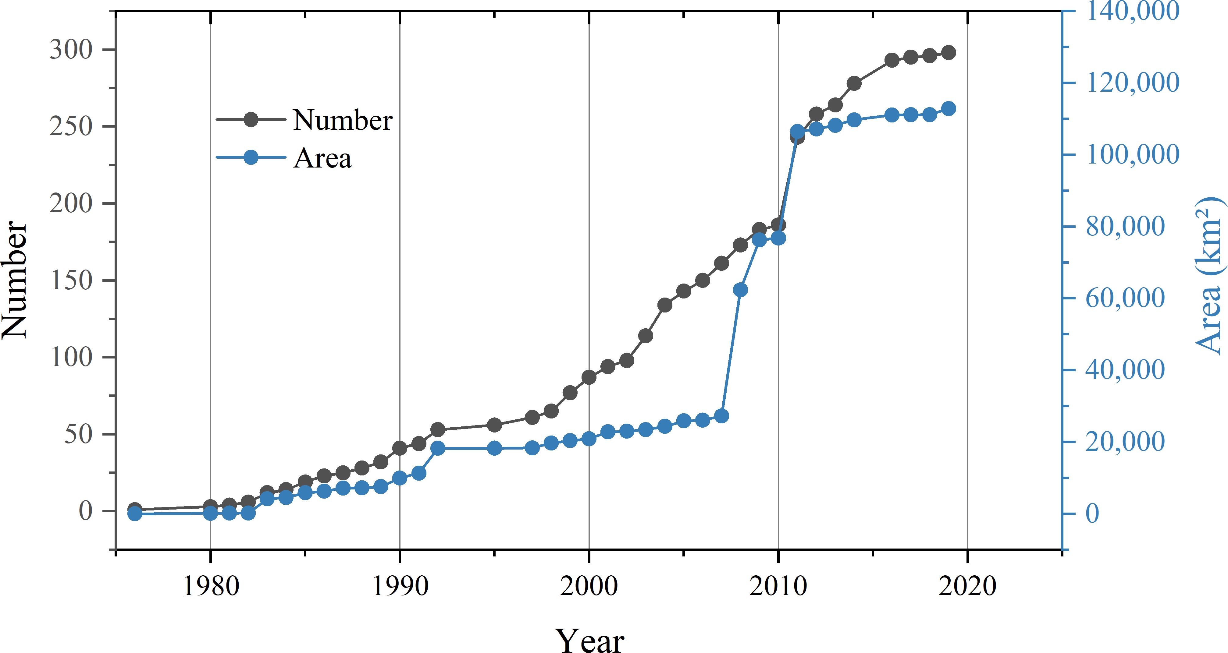
Figure 1. Development of MPA number and area in China, based on Bohorquez et al. (2021).

The establishment of MPAs can be understood from a public goods perspective under the social-ecological system (SES) framework (Ostrom, 1990; 2007; 2009; 2010a; b), where the resource-governance systems and units’ capabilities are weighed against shared benefits. Despite the scarcity of research on the determinants of MPA establishment in China, global scholars have applied generalized linear models to study cross-national factors such as space, economy and governance in building MPAs (Fox et al., 2012; Fouqueray and Papyrakis, 2019). Yet, these studies only focused on linear effects, often not involving ecological variables, nonlinear relationships and threshold effects, which are ubiquitous in socio-oceanographic systems (Popova et al., 2023; Chen et al., 2024; Chen and Xu, 2024b). These empirical, methodological and topical curiosities deserve more sophisticated framework, method and interpretations to advance the current understanding.

This article intends to address these issues by adaptively developing an SES-based theoretical framework of decision-making and extensively reviewing potential influencing factors of MPA establishment in spatial ecology and socioeconomics. Since most non-national-level MPAs in China are applied for and administered by municipal governments (Food and Agriculture Organization, 2024), data of 49 Chinese coastal cities that built MPAs during 1998–2020 were used for empirical verification. To overcome data issues, overdispersion-robust Poisson pseudo-maximum likelihood (PPML) regression with high-dimensional fixed effects (Correia et al., 2020) was adopted, with a mathematically based threshold algorithm to find the critical points where effects change. Among the determinants examined by the models, the effect of GDP revealed an N-shaped curve, supplementary to previous studies in the U-shaped environmental Kuznets curve, offering new insights of MPA establishment as a complex system.

Section 2 describes the theoretical framework and empirical methods used in this study, including spatial-ecological and socioeconomic foundations, empirical model specification and the threshold algorithm. It also describes the theoretical and empirical rationale for selecting specific indicators based on plentiful previous literature. Section 3 presents results of the full regression, threshold calculation and threshold regressions using the calculated tipping points. Section 4 discusses theoretical inference on the determinants, the N-shaped environmental Kuznets curve and threshold algorithm. Practical implications were drafted for balance between conservation and development, spatial-ecological and socioeconomic alignment and top-down adaptive governance. Section 5 draws the conclusions.

2 Framework and methods

2.1 Framework

Assuming that the region’s total MPA area is A, the species richness (number of species) within the area is S. The classical species-area relationship in ecology postulates $S=c{A}^z$ or $\ln S=\ln c+z\ln A$ (Matthews et al., 2019), where c is the number of species for one square unit and z is the rate of growth and usually $z<1$. This relationship applies to marine ecosystems (McDermott, 2021) and has been widely used to design MPAs (Terui et al., 2021). MPA benefits can be considered public goods shared by the total population P (Ban et al., 2015; Choi et al., 2020), where the total willingness to pay ($W_i$) for these benefits is:

$${{\displaystyle \sum }}_{i\in P}{W}_i=PS=Pc{A}^z$$

According to the SES theory (Ostrom, 1990; 2007; 2009; 2010a; b), the establishment of MPAs is subject to both resource and governance capacities. Suppose the MPA is fully planned and the number of spatial-ecological resources distributable to one species is R. Applying the concept of ecological connectivity, with every j-th new species introduced to the MPA, it can acquire resources from the former $j-1$ species through $j-1$ links. Therefore, the required new resource input is $R/j$. Summing over all species yields the total ecological resource requirement of ${{\displaystyle \sum }}_{j=1}^{S}R/j\approx R(\ln S+\gamma )$, the harmonic series with $\gamma$ being the Euler–Mascheroni constant. The logarithmic cost of dispersal is supported by literature in small species (Burkhalter et al., 2015), which is the case of many MPAs in China (Jiang and Jiang, 2023). Besides, the population P also demands spatial-ecological resources for sustainment, which is proportional to itself: bP. Substituting $\ln S$ with $\ln c+z\ln A$ yields:

$$a(\ln c+z\ln A+\gamma )+bP=N+M$$

where N is the amount of natural conditions (resource system) including water, nutrition, connectivity, and M is the land-sea space (resource unit). Although previous research found the establishment and operating costs of MPAs to be exponentially related to size (Balmford et al., 2004; Brander et al., 2020), the overall socioeconomic cost during resource allocation is logarithmic from a network and system perspective (Herald and Ramirez-Marquez, 2012; von Falkenhausen and Harks, 2013). According to the economies of scale, suppose the cost of building one unit area of MPA is C. When building the k-th unit area of MPA, due to the ability to use existing infrastructure and personnel from previous areas, the marginal cost is $C/k$. Therefore, the total socioeconomic cost of building A units of MPAs is ${{\displaystyle \sum }}_{k=1}^{A}C/k\approx C(\ln A+\gamma )$. Also considering the socioeconomic cost of maintaining the population dP, the equation for economic resource allocation becomes:

$$c(\ln A+\gamma )+dP=G+E$$

where c and d are parameters, G represents policy factors and E is the economy size, both rendered in comparable units. The ideal amount of A maximizes total willingness to pay while minimizes resource and governance costs, formulated by the Lagrange multiplier ($\mathcal{L}$):

$$\mathcal{L}(A,{\lambda }_1,{\lambda }_2)=Pc{A}^z+{\lambda }_1[a(\ln c+z\ln A+\gamma )+bP-N-M]+{\lambda }_2[c(\ln A+\gamma )+dP-G-E]$$

whose first-order derivative equations are:

$$\{\begin{array}{c}\frac{\partial \mathcal{L}}{\partial A}=Pcz{A}^{z-1}+\frac{1}{A}({\lambda }_{1}az+{\lambda }_{2}c)=0\\ \frac{\partial \mathcal{L}}{\partial {\lambda }_1}=a(\ln c+z\ln A+\gamma )+bP-N-M=0\\ \frac{\partial \mathcal{L}}{\partial {\lambda }_2}=c(\ln A+\gamma )+dP-G-E=0\end{array}$$

Solving the equations yields:

$$\ln A=\frac{1}{adz-bc}[d(N+M)-b(G+E)-ad\ln c-(ad-bc)\gamma ]$$

which means the logarithm of the total area (A) of MPAs is a linear combination (additive result) of spatial-ecological capacity ($N+M$) and socioeconomic capacity ($G+E$) (Figure 2). However, these relationships are not guaranteed to be always linear. The environmental Kuznets curve (EKC) implies that development-related variables may first inhibit environmental protection, then promote it when some threshold is crossed, while other variables could be the opposite (Wang et al., 2024c). Empirical methods are needed to address these threshold effects.

Figure 2

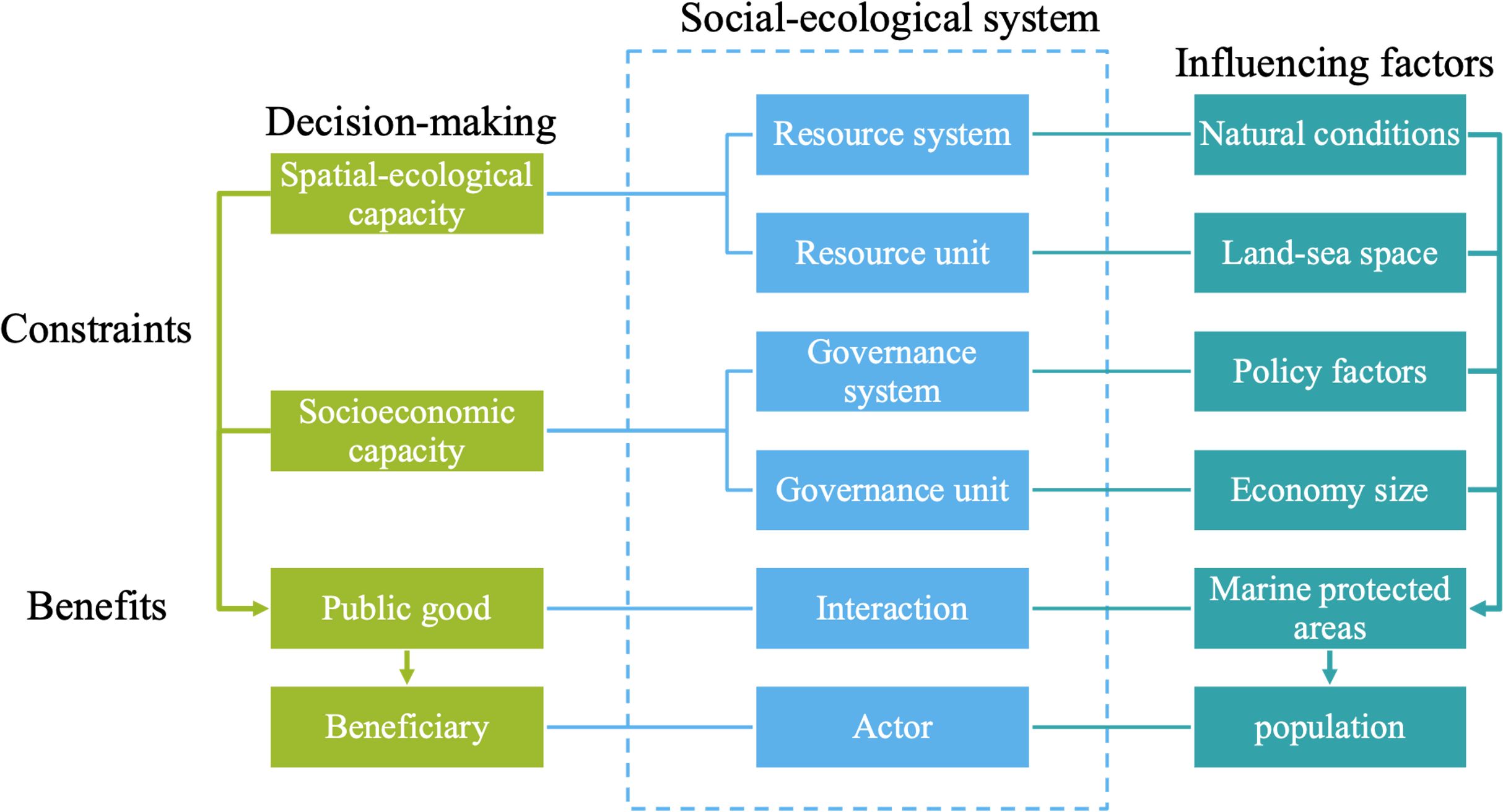
Figure 2. The SES-based MPA decision-making framework.

2.2 Methods

2.2.1 Empirical model

Although ecological studies suggest that species richness S in MPAs could be modeled using the Poisson distribution (Davies et al., 2022; Hoeksema et al., 2022; Espinoza et al., 2024), the area A of MPAs is usually not Poisson-distributed. Since $\ln A$ implies an additive relationship with spatial-ecological capacity ($N+M$) and socioeconomic capacity ($G+E$), its exponential form $A={\text{e}}^{x\beta }$ suggests a multiplicative relationship with $x={[1,N,M,G,E]}^{\text{T}}$ and $\beta$ being undetermined coefficients. To estimate the coefficients, the Poisson pseudo-maximum likelihood (PPML) regression with high-dimensional fixed effects (HDFEs) is adopted (Santos Silva and Tenreyro, 2006; Correia et al., 2020), which can pertain to any nonnegative data (including non-count data with zeros) without needing to assume a specific distribution (e.g., Poisson). The method is robust to distributional misspecification such as overdispersion, zero-inflation, heterogeneity and heteroskedasticity. Since the method relies on pseudo-maximum likelihood (PML) principles, consistent and unbiased estimates only require correct specification of the conditional mean structure: $E(y_i|x_i)={\mu }_i={\text{e}}^{x_i\beta }$, which is ensured by the theoretical deduction.

Despite originating from spatial econometrics of international trade, the PPML method has been widely adopted in many area-based geographic analyses, such as land size (Lay and Nolte, 2017; Anti, 2022; Raimondi and Scoppola, 2022). One of its advantages at addressing spatiotemporal problems is the ability to construct HDFEs to represent latent spatial and network autocorrelation (Gu et al., 2022, 2023, 2024). Additionally, it allows for cluster robust standard errors to account for autocorrelation in the variables (Anderton and Anderton, 2021; Ding et al., 2025; Long et al., 2025). In environmental planning and management, scholars found PPML to be superior to spatial Durbin models with higher probability of finding significant impacts of climate factors by using more granular data (Ton et al., 2024), providing more information about the mechanisms behind the effects with advanced accuracy of the estimated coefficients. It also performs better than geographically weighted regression (GWR) models in avoiding heteroskedasticity (Ko et al., 2022).

Previous research has noted the potential endogeneity between protected areas and establishment costs in China, such as opportunity costs for local communities or industries (Yang and Wu, 2022). However, the ideal instruments to address MPA endogeneity are difficult to identify, and incorporating instrumental variable estimators with fixed effects in PPML evokes the incidental parameter problem, leading to inconsistent estimates (Santos Silva and Tenreyro, 2022). Following empirical studies in econometrics and ecological economics (Baier and Bergstrand, 2007; Weidner and Zylkin, 2021; Peiró-Palomino et al., 2022), the article adopted three-way fixed effects on province, municipal and temporal levels to absorb time-varying factors like policy changes, economic conditions, or shifts in political power, and time-invariant path-dependence factors such as regional preferences for conservation, institutional capacity, or geographical conditions.

According to Article 12 of the Regulations of the People’s Republic of China on Nature Reserves effective during 1994-today (the 1994 Regulations, for short), the province is tasked with applying for national protected areas, while municipal governments can apply for local ones (Food and Agriculture Organization, 2024). Considering that the establishment of MPAs in China is coordinated by provincial and municipal factors (Wang et al., 2025b) as well as time trends (Bohorquez et al., 2021), the study also incorporates high-dimensional fixed effects for the province (${\pi }_i$), city (${\sigma }_i$) and year (${\tau }_t$) to absorb the effects of omitted variables due to unobserved provincial, municipal and temporal heterogeneity (Yao et al., 2025).

Previous studies used year $t-1$ independent variables to explain China’s protected areas in year t based on the policy lag premise (Yang and Wu, 2022). However, using lagged independent variables (lagged predictors) in panel data analysis with fixed effects risks potential biases or misleading results (Vaisey and Miles, 2017), even obscuring the true causal mechanisms when the correct lag structure is not properly specified (Leszczensky and Wolbring, 2022). Moreover, studies found China’s nature reserves to be subject to ad hoc policy changes or project demands such as the construction of ports, industrial zones, and infrastructure (Ma, 2016; Ma et al., 2019), which are best reflected in socioeconomic indicators of the same year. Besides, climatological predictors are instantaneous (Nordio and Fagherazzi, 2022) and exogenous (Wang et al., 2022) in protected areas. Consequently, no lags were applied to variables in the study, as in other PPML studies on contemporaneous effects (von Laer et al., 2022; Ekanayake et al., 2023; Friedmann and Pedersen, 2024; Giorgi et al., 2025) and studies on determinants of protected areas (Sims, 2010; Fox et al., 2012; Opršal et al., 2018; Fouqueray and Papyrakis, 2019; Mance et al., 2021; Bareille et al., 2023).

Since previous studies found in welfare economics that the odds of building protected areas are linearly tied to the net social benefit decided by the difference between total benefit and costs (Wu and Liu, 2012; Yang and Wu, 2019), the number of MPAs (n) is also used as an alternative to $\ln A$. This is equivalent to the identify link function $g(\mu )=\mu =X\beta$ instead of the more often used log link function $g(\mu )=\ln \mu =X\beta$ in general linear models (GLMs), but it is equally effective under nonnegativity constraints and may generate a better fit in biometrics and ecology (Lu et al., 2022; Pinheiro et al., 2022; Heit et al., 2024). The use of the exponentiated number of MPAs is further bolstered by previous research on the log-log linear relationship between MPA number and area (Fox et al., 2012), which is equivalent to exponentiality. As the original dependent variable data, it takes the exponential form. With $y_{i,t}=A_{i,t}$ or ${\text{e}}^{n_{i,t}}$ being the dependent variable, the final empirical model can be written as:

$$\ln y_{i,t}={\beta }_0+N_{i,t}{\beta }_N+M_{i,t}{\beta }_M+G_{i,t}{\beta }_G+E_{i,t}{\beta }_E+{\pi }_i+{\sigma }_i+{\tau }_t+u_{i,t}$$

where ${\beta }_0$ is the constant; $N_{i,t}$, $M_{i,t}$, $G_{i,t}$ and $E_{i,t}$ are the time-variant $1\times k$ spatial-ecological and socioeconomic variable factors for city i in year t; ${\beta }_N$, ${\beta }_M$, ${\beta }_G$ and ${\beta }_E$ are the corresponding $k\times 1$ parameters; $u_{i,t}$ is the error term. The empirical model also utilizes robust standard errors that can produce more rigorous results than traditional panel Poisson regressions (Santos Silva and Tenreyro, 2006; 2011; 2022).

2.2.2 Threshold calculation

The threshold calculation is based on the threshold regression developed by Hansen (1999; 2000). However, since currently no statistical packages are designed for threshold calculation in PPMLHDFE models, the study adopts a modified grid search algorithm to determine the threshold θ where coefficients change course. Suppose the estimated coefficient of independent variable x is $\beta$, then the algorithm splits x into two parts: $x\le \theta$ and $x>\theta$ to estimate the two parts separately with the same empirical model. To avoid missing critical values or depleting datasets, θ ranges from the 25th percentile ($Q_1(x)$) to the 75th percentile ($Q_3(x)$) of x, until the true threshold θ^* is found. In practice, a discrete approach was adopted, by adding a minuscule increment each time from $Q_1(x)$ to $Q_3(x)$.

As $\beta =f(\theta )$ is a function of the threshold range θ, the three concrete conditions for true threshold θ^* are: (1) Local extremity. According to the mathematical definition of an extremum, $f(\theta )$ has a local relative maximum (or minimum) point at θ^*, if for all θ within distance $ϵ>0$ of ${\theta }^{*}\in [Q_1(x),Q_3(x)]$, there are no $f(\theta )$ values larger (or smaller) than $f({\theta }^{*})$; (2) Forward extremity. For all $Q_3(x)\ge \theta >{\theta }^{*}$, $f(\theta )$ should be smaller (or larger) than $f({\theta }^{*})$, meaning that no forward values can surpass the current coefficient in terms of extreme high or extreme low; (3) Transcendentality. Finally, for a sufficiently small diameter $\delta \to 0$, there exists one point within the neighborhood $[{\theta }^{*}-\delta ,{\theta }^{*}+\delta ]$ of θ^* where the 95% confidence intervals of $f(\theta )$: ($C{I}_{95\%}(f(\theta \pm \delta ))=[L{B}_{95\%}(f(\theta \pm \delta )),U{B}_{95\%}(f(\theta \pm \delta ))]$) should be on different sides of the axis to represent the transition from one regime to the other. The three key conditions for θ^* can be compactly formulated as:

$$\{\begin{array}{c}\exists ϵ>0((f({\theta }^{*})\ge f({\theta }^{*}\pm ϵ))\vee (f({\theta }^{*})\le f({\theta }^{*}\pm ϵ)))\\ \forall \theta \in ({\theta }^{*},Q_3(x)]((f(\theta )<f({\theta }^{*}))\vee (f(\theta )>f({\theta }^{*})))\\ \exists \delta >0(L{B}_{95\%}(f(\theta \pm \delta ))U{B}_{95\%}(f(\theta \pm \delta )))<0\end{array}$$

where the left conditional branch indicates a downward threshold effect, while the right branch indicates an upward effect. The left branch does not interfere with the right branch because the conditions are mutually exclusive. In practice, $\delta$ was set as 5% of the grid search interval: $Q_3(x)-Q_1(x)$. After determining the supposed threshold ${\theta }^{*}$, the coefficients should be significant for both $x\le {\theta }^{*}$ and $x>{\theta }^{*}$ to formalize it as the true threshold.

2.3 Data sources and statistics

2.3.1 MPA area and number

The area and number of MPAs are from the compiled list by Bohorquez et al. (2021), currently the most comprehensive database on area-based marine conservation in China. After cleansing, a total of 288 MPAs (123,891 km²) were included, corresponding to 49 prefecture-level coastal cities. MPAs built in provincial directly-governed county-level cities were excluded due to difficulty in attributing data. Following previous studies, the total or cumulative area (Fox et al., 2012; Wu et al., 2018; Yang and Wu, 2022) and number (Fox et al., 2012) of MPAs were used and interpolated linearly. Given the log link for $A_{i,t}$ ​ and the identity link for $n_{i,t}$, the coefficients capture semi-elasticity for both proportional and absolute changes in the dependent variable resulting from a one-unit independent variable increment.

2.3.2 Natural conditions

Natural conditions (resource system) N, such as precipitation ($Precip$), wind speed ($Wind$) and urban green space ($Green$), can be reflective of the underlying resource system. According to the ecosystem pulse theory (Souto-Vieira et al., 2024), precipitation can increase species richness, abundance, taxonomic, phylogenetic and functional biodiversity of fish assemblages in neritic zones (da Silva et al., 2021) through the estuarization process (Macedo et al., 2021) as deep as 30 m (Passos et al., 2016). The effect works in several ways, first through the influx of freshwater that supports certain estuarine species, such as polychaeta, isopoda, crustaceans (Checon et al., 2023) by regulating salinity levels, enhancing habitat connectivity and facilitating species movements (da Silva et al., 2021). It also drives biomass exchange between estuarine and marine ecosystems (Macedo et al., 2023). Second, freshwater runoff from terrestrial sources brings in nutrients that can stimulate primary and secondary production in estuarine environments, increasing the trophic complexity, resilience and maturity (Macedo et al., 2023). Third, rainfall can trigger migration and breeding behaviors in fish, allowing for organic matter and energy transfer and creating a trophic meta-ecosystem convergence (Macedo et al., 2021). Since the majority of China’s MPAs are in shallow and medium waters, hourly observed climatology data for precipitation (mm) from the National Centers for Environmental Information (NCEI) (2023) divided by 10 is used as a predictor of natural condition and MPA establishment, by averaging the yearly indicators from each city’s weather stations.

Wind also affects marine organisms by enhancing marine connectivity, inducing coastal upwelling, transporting fish larvae and accelerating migration and recruitment (Arteaga et al., 2024; Suca et al., 2025). First, wind-driven surface connectivity and circulation influence the distribution of nutrients and organisms in marine environments (Xu et al., 2023a). Strong winds can also cause nutrient-rich water to circulate and support the growth of phytoplankton and other marine species (Moore-Maley and Allen, 2022). Second, wind-induced vertical upwelling generates high biological productivity due to nutrient enrichment of the surface layers to stimulate primary and secondary productivity, which has been intensifying in the four China Seas during 1982-2020 (Wang et al., 2021; Liu et al., 2023; Luo et al., 2023; Xu et al., 2023b). This increased productivity facilitates the boom of phytoplankton, other primary producers and finally fish (Bai et al., 2020). Third, wind-driven transport of larval fish has been reported in various literature (Schilling et al., 2022; Šmejkal et al., 2023; Arai and Kimura, 2024). Therefore, city-average wind speed data (m/s) from NCEI divided by 10 is included as a positive factor.

Urban green space can also reflect MPA development through several theoretically and empirically verified pathways. First, as a nature-based solution (NbS), urban green space directly absorbs rainwater and stormwater run-off (MacKinnon et al., 2019), which is a major contamination source for aquatic and coastal ecosystems (Werbowski et al., 2021; Lapointe et al., 2022). Features like green roofs, bioretention systems, and constructed wetlands also help in improving air quality to eventually favor adjacent marine ecosystems like mangroves, seagrass meadows and salt marshes (Pinto et al., 2023; Sun et al., 2024)​, especially providing cooling under climate change and extreme events (Li et al., 2024b). Second, urban green space development increases the planning ability and experience of the city through path dependence (Addas, 2023; Bille et al., 2023), which also furthers later development in MPAs. Third, urban green space extends ecological corridors in fragmented coastal habitats connecting MPAs and other effective area-based conservation measures (OECMs) (Podda and Porporato, 2023). The integration of green space and marine ecosystems is pronounced in water cycles (Yuan and Kim, 2024). Considering these effects, urban green area (100 km²) of the municipal district from China City Statistical Yearbook (CCSYs) is used as a positive factor.

2.3.3 Land-sea space

Land–sea space (resource unit) M is reflected in maritime passenger traffic ($Traffic$), population density ($Density$) and built-up area ($Built$). Larger maritime traffic flow is a reflector of the size of sea space, which provides more ample room for the existence of an MPA (Yap and Loh, 2019). While maritime traffic is often associated with negative impacts on marine ecosystems, such as habitat disturbances, higher vessel density might in turn invoke conservation measures due to raised awareness and economic growth based on the EKC, as witnessed by international empirical studies on marine transport sectors (Go et al., 2021; Kalaycı and Özden, 2021; Pata et al., 2023). These theoretical and empirical foundations support using maritime traffic (10 million) from CCSYs as a positive factor. On the other hand, coastline length may also be related to MPA development, but some cross-national evidence reported insignificant effect on the spatial extent of MPAs (Fox et al., 2012; Fouqueray and Papyrakis, 2019). Moreover, literature also suggests countries with limited coastlines may prioritize MPAs due to scarcity value (Horowitz, 2002). Therefore, coastline is not adopted as the sea space variable.

Higher population density in surrounding coastal areas can result in increased anthropogenic pressures on MPAs. It can lead to intensified fishing, pollution, coastal development, and habitat destruction, which can threaten the effectiveness and conservation goals of the MPA (Mascia et al., 2017). As human populations grow, especially in coastal areas, the competition for marine resources, such as fishing and tourism, intensifies, which may reduce the political will or capacity to implement MPAs and has been observed in various cross-national empirical studies (Sims, 2010; Opršal et al., 2018; Wu et al., 2018; Fouqueray and Papyrakis, 2019; Yang and Wu, 2022). Therefore, municipal-level population density (1000/km²) from CCSYs is included as a negative factor.

The extent of coastal construction and urbanization can directly impact available habitat and ecological connectivity within and around MPAs (Bulleri and Chapman, 2010). It is noteworthy that this impact pertains to not only marine construction, but also inland built-up areas. Studies identified high pressure of built-up areas on protected coastal areas such as mangroves or salt marshes due to fragility, vicinity and vulnerability (Romañach et al., 2018; Fuente et al., 2020). The urban expansion, along with sea level rise, constitutes the coastal squeeze faced by many habitats along global coastlines (Kirwan and Megonigal, 2013; Smart et al., 2021; Lansu et al., 2024). Hence, built-up area (100 km²) of the municipal district from CCSYs is used as a negative factor.

2.3.4 Policy factors

Policy factors (governance system) G are reflected in the number of scientific and technological personnel ($Tech$), infrastructure investment ($Infra$) and cultural promotion presented by the number of public library books ($Book$). Scientific and technological personnel, including protected area professional staff, are critical for MPA development (Appleton et al., 2022). According to the Marine Eco-Environmental Protection in China White Paper of The State Council Information Office (2024), China is committed to innovation in marine eco-environmental protection technologies, monitoring and evaluation, and institutions and mechanisms. It has made rational decisions and implemented targeted measures to transform and advance protection through digital and smart technology. Therefore, the number of scientific and technological personnel (10,000) from CCSYs will be directly indicative of each city’s policy alignment with the central government and technological power to enhance marine conservation.

Although there might be some competition for funding between urban infrastructure and MPAs (Jaffé et al., 2025), the overall impact of infrastructure investment is beneficial to MPAs. Infrastructure provides basic physical conditions for MPAs to operate (Cao et al., 2021). Furthermore, infrastructure can buffer extreme natural events from intruding marine ecosystems, such as rainstorms, effectively acting as a separation wall (Giang and Khanal, 2024). Infrastructure investment is representative of the government’s building capacity and efficiency (Geng and Lo, 2024). Finally, well-regulated infrastructure can spill over to MPA development through network externality and synergy (Roberts et al., 2023; Gong et al., 2024). Consequently, the yearly investment amount completed in urban environmental infrastructure construction (¥10 billion) from CCSYs is used as a positive factor. Since nominal infrastructure investment is directly related to the cost of building MPAs, it was not deflated.

Library books have long been an effective tool for building environmental management capacity opportunities in literature (Devine and Appleton, 2023; Phaka et al., 2023; Aregbesola et al., 2024). Public library books can promote and implement citizen science initiatives (Cigarini et al., 2021; Walker et al., 2023; Mumelaš and Martek, 2024), which helps to disseminate conservation awareness, increase social cohesion, and improve residents’ acceptance towards MPAs. Moreover, at the macro level the number of books in public libraries is indicative of a city’s cultural orientation, which is related to the degree of official focus on conservation (Jenkins, 2022; Andersson et al., 2024). Therefore, despite the digital age, the number of books in public libraries has been extensively used and verified in recent empirical studies to represent the sociocultural factor, especially in China (Xia and Zhai, 2022; Dong et al., 2023a, b; Zhang et al., 2025). Although other studies used national educational expenditure as an MPA predictor (Fouqueray and Papyrakis, 2019), this study uses each city’s public library books per capita from CCSYs instead.

2.3.5 Economy size

Economy size (governance unit) E is reflected in the output ($GDP$), demand ($Pop$) and supply ($Export$). Although the MPA establishment in China is often state-driven, tied to centralized fiscal policies (e.g., Five-Year Plans) (Hu et al., 2020) or local government performance metrics (e.g., ecological civilization targets), funding from the central government only accounts for a limited portion of the overall budget, and a large amount of funding for protected areas is supported by local financing, especially for non-national-level local protected areas (He and Cliquet, 2020). Since the 1994 Regulations give local governments the authority to apply for MPAs based on their situations (Food and Agriculture Organization, 2024), the total economic output (GDP) is included as a predictor of MPA establishment, as seen in previous studies of China’s protected areas (Yang and Wu, 2022). Some international studies used GDP per capita (Fouqueray and Papyrakis, 2019; Mance et al., 2021) or HDI (Fox et al., 2012; Opršal et al., 2018; Mance et al., 2021) as determinants, but based on China’s collectivist nature in cultural dimensions (Hofstede, 2011), it may be better suited by GDP (¥ trillion) from CCSYs as a whole (Yang and Wu, 2022). Since nominal GDP is directly related to the cost of building MPAs, it was not deflated in regressions, following other studies (Hao et al., 2022; Wang et al., 2024a; Zhou, 2024; Ulate et al., 2025), where inflation effects are also absorbed by time-varying high-dimensional fixed effects (Jaravel and Sager, 2019; Kunofiwa, 2022). The threshold analysis, however, used 1998-based deflators of each city’s province from the Stata module “cngdf” (Song, 2021) to calculate real $GDPr$, the most accurate GDP deflator available for Chinese cities.

Besides population density (Sims, 2010; Fouqueray and Papyrakis, 2019; Yang and Wu, 2022), the total population in the vicinity of MPAs can also influence the demand for marine resources and coastal activities (Fox et al., 2012), with some studies using density and total population simultaneously (Opršal et al., 2018). As the empirical results of Opršal et al. (2018) demonstrate, total population significantly predicts more protected areas. Since in China, population-growing areas tend to have younger population structures through immigration (Gu and Xu, 2022; Gu et al., 2022b), the younger generations create higher demands for both nature-friendly economic development and ecological conservation, and they are more open to the concepts of MPAs (Turnbull et al., 2021). According to the urban scaling theory, the relationship between total population and density in Chinese cities is not perfectly collinear (Tan et al., 2025), thus the yearly average population (million) of each city from CCSYs is used as a positive factor.

Regions heavily dependent on exports may prioritize economic growth over environmental conservation, leading to a lack of investment in MPAs (Acheampong and Opoku, 2023). Wang et al. (2024b) examined the impact of export expansion on local environment in China during 2000–2020 and found regions with larger export expansion experienced more pronounced initial environmental deterioration. The inclusion of exports (¥ trillion) from CCSYs in the model corresponds to the south-north diversity of export-orientation in China’s coastal cities (Li et al., 2022; Chen and Xu, 2024d) due to the Maritime Silk Road (Li et al., 2024a), which is less obviously conveyed by GDP. Since exports are an inflated reflector of real goods, they were adjusted using provincial GDP deflators with 1998 as the base year.

2.3.6 Descriptive statistics

The descriptive statistics covering a total of 23 years, 49 cities and 49×23 = 1127 samples are shown in Table 1. The start point of 1998 is due to multiple historical and statistical facts. Internationally, the United Nations proposed “International Year of the Ocean” in 1998. Domestically, the Outline of the Planning of Nature Reserve Development of China (1996–2010) required local governments to complete nature reserves planning by July 1998. The same year, the State Oceanic Administration merged into the newly established Ministry of Land and Resources to supervise ocean management, which saw an instant boost of MPA number and area (Figure 1). Several important ocean laws and regulations (e.g., GB/T17504-1998) were also promulgated that year. The end year of 2020 is attributed to China’s early completion of the Aichi Biodiversity Targets to conserve 12.98% of the seas (Bohorquez et al., 2021), which led to a slowdown. Besides, the COVID-19 pandemic post 2020 also decelerated MPA construction. Missing data were extended to 1998–2020 using the fittest ARIMA models.

Table 1

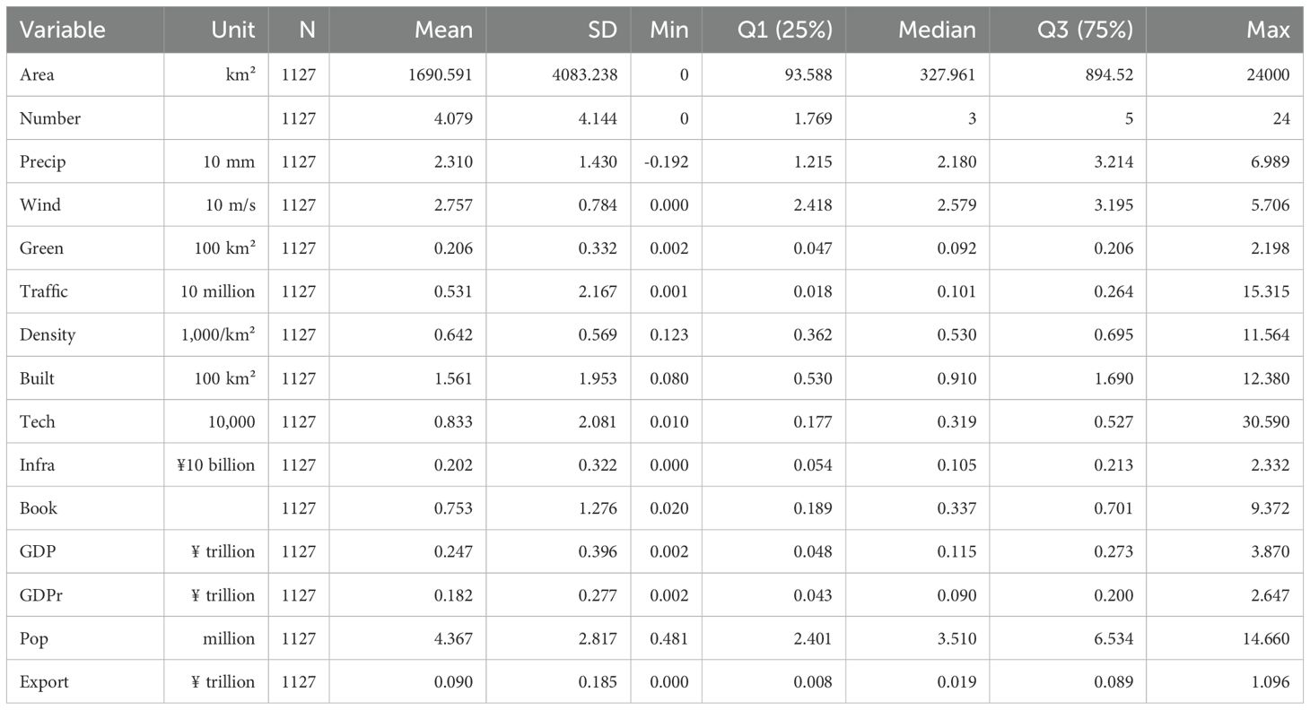
Table 1. Descriptive statistics of variables.

Using the Stata module “coldiag2” (Hendrickx, 2004), the condition number of variables is 17.64<30, indicating no high multicollinearity issues. The study also explicitly tested the overdispersion of the dependent variables $A_{i,t}$ and ${\text{e}}^{n_{i,t}}$ using the Stata module “overdisp” without previously estimating Poisson or binomial negative models (Fávero et al., 2020). The coefficients of $\widehat{u}=E(y_i|x_i)$ in $Var(y_i|x_i)=\widehat{u}+\alpha {\widehat{u}}^2$ were 2.62 (p<0.001) and 0.47 (p<0.001) and rejected the equidispersion hypothesis, demonstrating the necessity of using the PPMLHDFE model to robustly estimate overdispersal data. According to Santos Silva and Tenreyro (2011), the PPML estimator with 1000 samples is robust with only <3.5% bias even when $Var(y_i|x_i)=3E(y_i|x_i)+30E{(y_i|x_i)}^2$, which is close to the sample size (1127) in this study. Other studies also support using PPML instead of negative binomial regression under strong overdispersion (Head and Mayer, 2014; Curzi and Huysmans, 2022; Saussay and Sato, 2024).

3 Results

3.1 Spatiotemporal distribution

Figure 3 shows the development of Chinese MPAs in the last two decades (2000-2019) can be divided into four stages. During the first stage (2000-2004), most cities had 1 to 5 MPA each, and only the city of Zhanjiang had more than 10 MPAs. Most MPA areas were under 5,000 km², with one exception, and most of them were settled in the south. In the second stage (2005-2009), two cities emerged, Zhanjiang and Yangjiang, with more than 10 MPAs, and there were four MPAs with areas larger than 10,000 km² from north to south, making the spatial distribution more balanced. The third stage (2010-2014) set a milestone in the quantitative and qualitative development of MPAs, where Zhanjiang and Yantai achieved more than 20 and four other cities exceeded 10. Large-scale MPAs became more common along the coastline and the largest MPA thus far (23,219 km²) had appeared. Compared to the rapid progress in stage three, the fourth stage (2015-2019) is more conservative, with only 18 newly built cities, mostly in cities already with more than 10 MPAs.

Figure 3

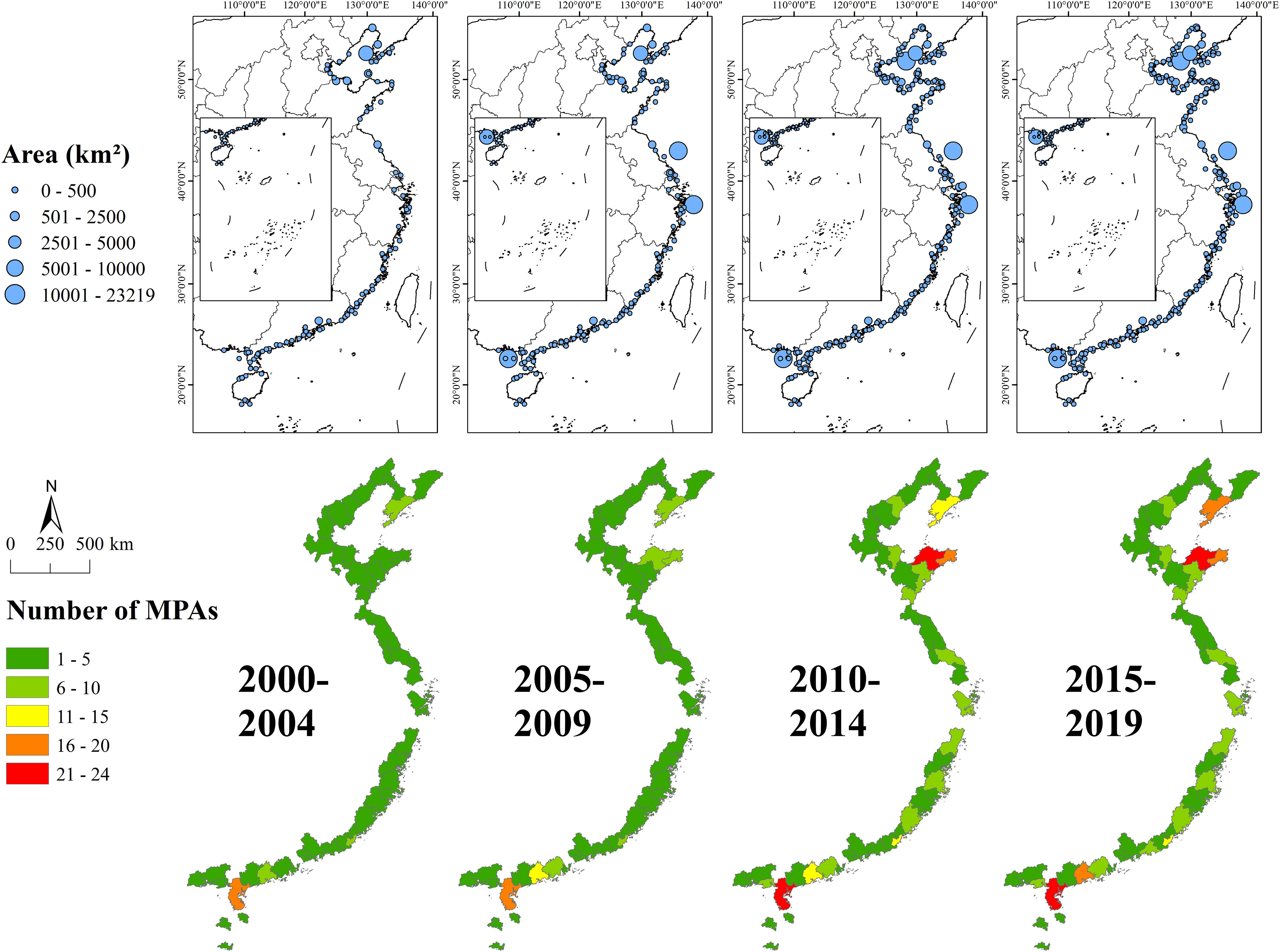
Figure 3. Spatiotemporal evolution of MPA distribution in Chinese coastal cities.

The local Moran’s I for MPA size indicates that there is significantly (p<0.05) positive but slight (0.084) spatial correlation, with the Bohai Sea and Yangtze River Delta being the two aggregation centers, and the high-high parts are mainly in the Yangtze River Delta. Local Moran’s I for MPA number also indicates a significantly (p<0.05) positive and larger (0.118) spatial correlation, with the Bohai Sea and Pearl River Delta being the two aggregation centers, and the high-high parts are mainly situated along the Bohai Sea.

3.2 Full regression

Table 2 shows averagely MPA size grows ${\text{e}}^{0.066}-1=6.82\%$ each year with the time trend. Wind speed consistently shows a positive and statistically significant effect across all four models, with particularly strong coefficients in the models explaining the number of MPAs (Models 3 and 4), reaching as high as 2.950 (p<0.001). This indicates that higher wind speeds may be associated with both larger areas and greater numbers of MPAs, verifying the enhancement of wind on marine ecosystems. Green space ($Green$) also demonstrates a robust and positive influence, significant at the 1% level in Models 1, 2 and 3, suggesting that urban green coverage is a meaningful proxy for environmental considerations and improvement in MPA establishment. However, precipitation ($Precip$) shows weak and mostly insignificant effects, with significance only emerging in Model 4 (0.619, p<0.001). Averagely, 10 km² more urban green space makes MPA size ${\text{e}}^{2.046\times 0.1}-1=22.70\%$ to ${\text{e}}^{4.089\times 0.1}-1=32.34\%$ larger, or adds 0.47 more MPAs.

Table 2

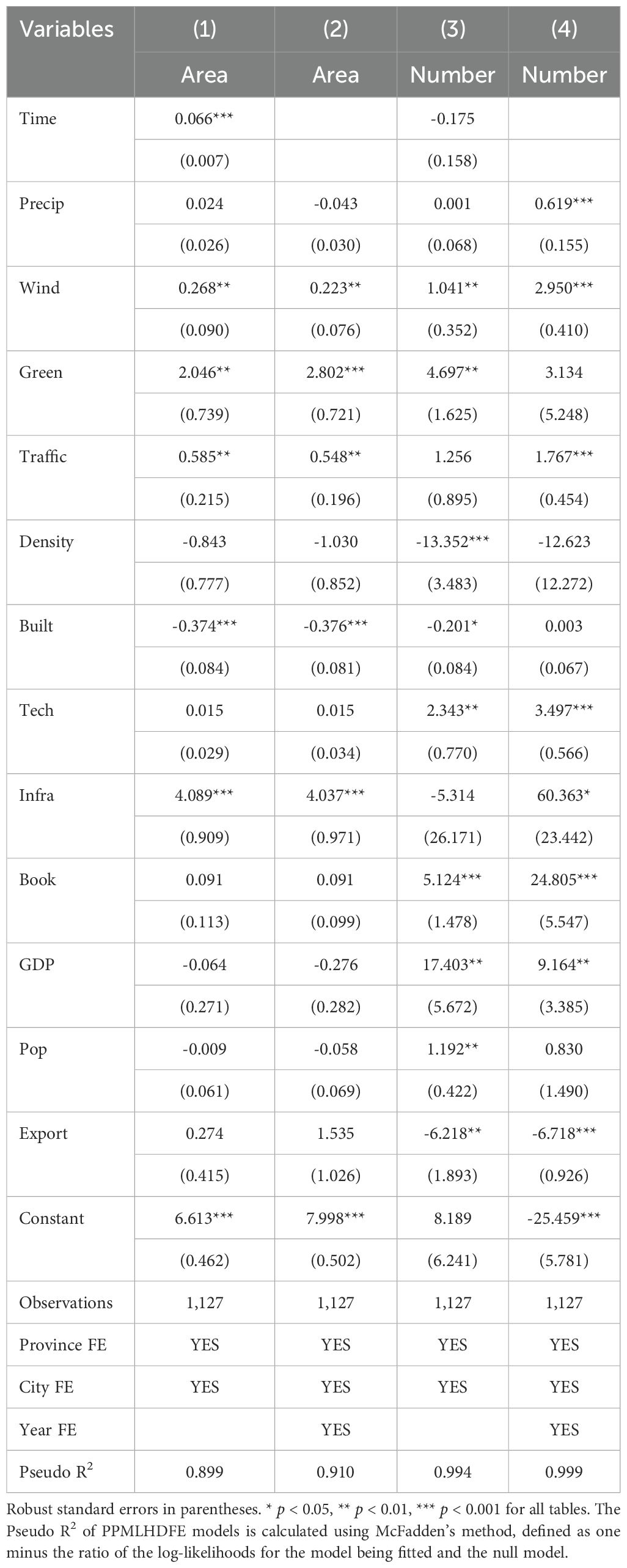
Table 2. Full regression results.

Maritime traffic ($Traffic$) is positively associated with MPAs, being significant in all area models and especially in Model 4 (1.767, p<0.001), which suggests that increased maritime movement encourages more and larger MPAs, possibly due to higher monitoring needs or conservation pressures. Density, by contrast, exhibits a negative effect in Models 3 (-13.352, p<0.001), highlighting that higher population density may constrain the establishment of MPAs, particularly in terms of their number. Built-up area ($Built$) shows a negative and robust association with area-based models (-0.374 and -0.376 in Models 1 and 2, both p<0.001), as well as in Model 3 (-0.201, p<0.05).

Infrastructure investment ($Infra$) stands out with large positive effects on area-based models (4.089 and 4.037 in Models 1 and 2, both p<0.001), and an exceptionally large coefficient in Model 4 for the number of MPAs (60.363, p<0.05), underlining the importance of government investment in supporting conservation infrastructure. Technological personnel ($Tech$) shows a positive and significant effect in Model 3 (2.343, p<0.01), suggesting that a higher number of scientific and technological personnel facilitates the creation of more MPAs. Cultural promotion ($Book$), proxied by the number of books, is significant and positive in the number-based models, particularly in Models 3 and 4 (5.124 and 24.805, both p<0.001). Averagely, investing ¥1 billion in infrastructure increases MPA size by ${\text{e}}^{4.037\times 0.1}-1=49.74\%$ or ${\text{e}}^{4.089\times 0.1}-1=50.52\%$, while increasing 10 thousand technological personnel boosts MPA number by 2.343 to 3.497.

GDP positively affects the number of MPAs, with significant coefficients in Models 3 (17.403) and 4 (9.164), both p<0.01 and suggesting that wealthier regions are more likely to establish MPAs. Population ($Pop$) shows a positive and significant effect in Model 3 (1.192, p<0.01) but becomes insignificant in other models, indicating that population demand may drive MPA numbers only under certain conditions. Interestingly, exports ($Export$) demonstrate a negative and significant effect on the number of MPAs in Models 3 (-6.218, p<0.01) and 4 (-6.718, p<0.001), implying a possible trade-off between economic openness and conservation priorities. In contrast, these economic variables are generally insignificant in explaining the area of MPAs (Models 1 and 2). The variable coefficients of $GDP$, $Built$ and $Traffic$ merit further threshold analysis to determine the key point of taking effects on area.

3.3 Threshold analysis

3.3.1 GDP

The N-shaped curve in Figure 4 features a critical real GDP value of ¥55 billion (1998-based, equal to ¥106.5 billion in 2020), which indicates a significant shift in the relationship between GDP and MPA size. Below this threshold, the effect on MPA size appears to be negative, with the coefficient values being low or even negative. However, above the threshold, the effect on MPA size becomes positive and increases gradually, as shown by the rising coefficient values. The shaded area represents the 95% confidence intervals (CI), which show considerable uncertainty below the threshold, but as the GDP rises, the confidence intervals become narrower, suggesting more certainty in the positive relationship between GDP and MPA size.

Figure 4

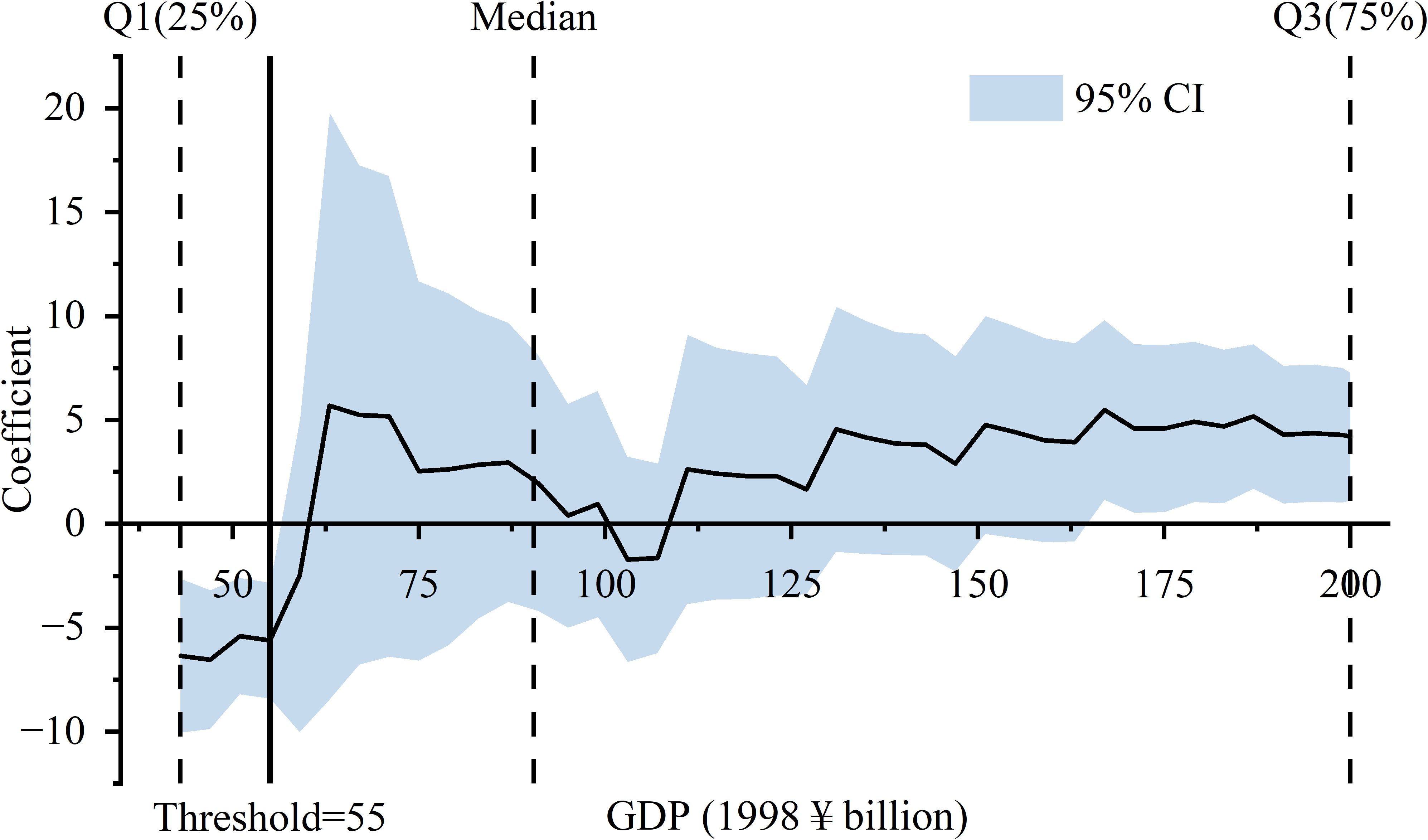
Figure 4. Threshold plot of the effect of GDP.

Table 3 displays threshold regression results with control variables hidden, where Models (1) with real GDP≤¥55 billion, has a significant negative (-5.611, p<0.001) coefficient. In contrast, Models (3) and (4), with real GDP>¥55 billion, show a positive and significant relationship (0.512, p<0.001). This shift suggests a marked change in the effect of GDP on MPA size at the ¥55 billion threshold. The Pseudo R² values suggest a strong fit, confirming the robustness of the regression results. Increasing nominal GDP by ¥1 trillion results in ${\text{e}}^{0.512}-1=66.86\%$ increase in MPA size.

Table 3

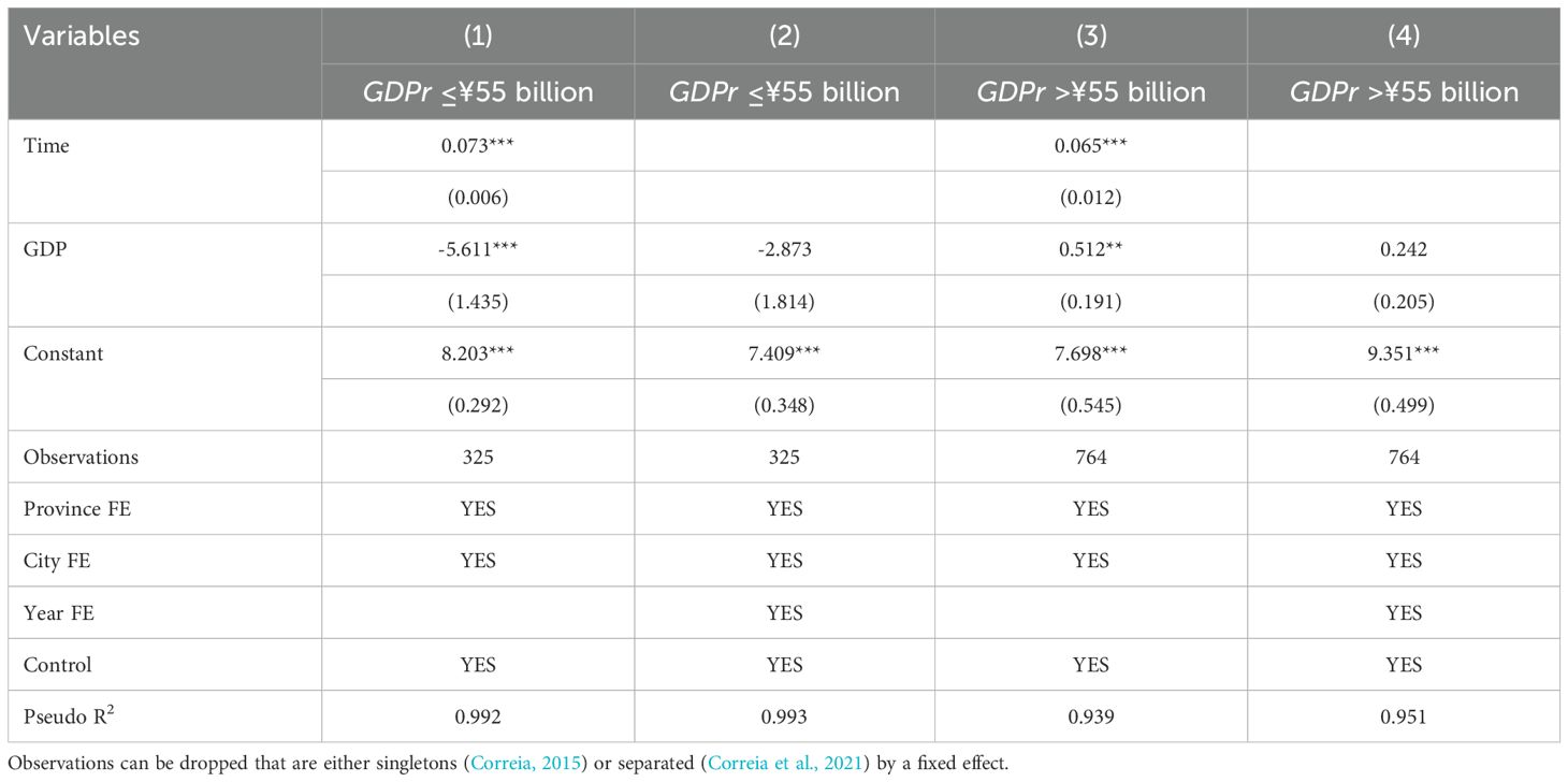
Table 3. Threshold regression results of the effect of GDP.

3.3.2 Built-up area

Figure 5 demonstrates an N-shaped curve, with a slightly positive relationship before the threshold of 63 km², suggesting that as built-up areas increase, the size of marine protected areas tends to grow. However, once the built-up area exceeds this threshold, the relationship becomes negative, indicating that further urbanization leads to a decrease in the size of marine protected areas. This suggests that in more urbanized regions, competing land use pressures may restrict the establishment of larger MPAs.

Figure 5

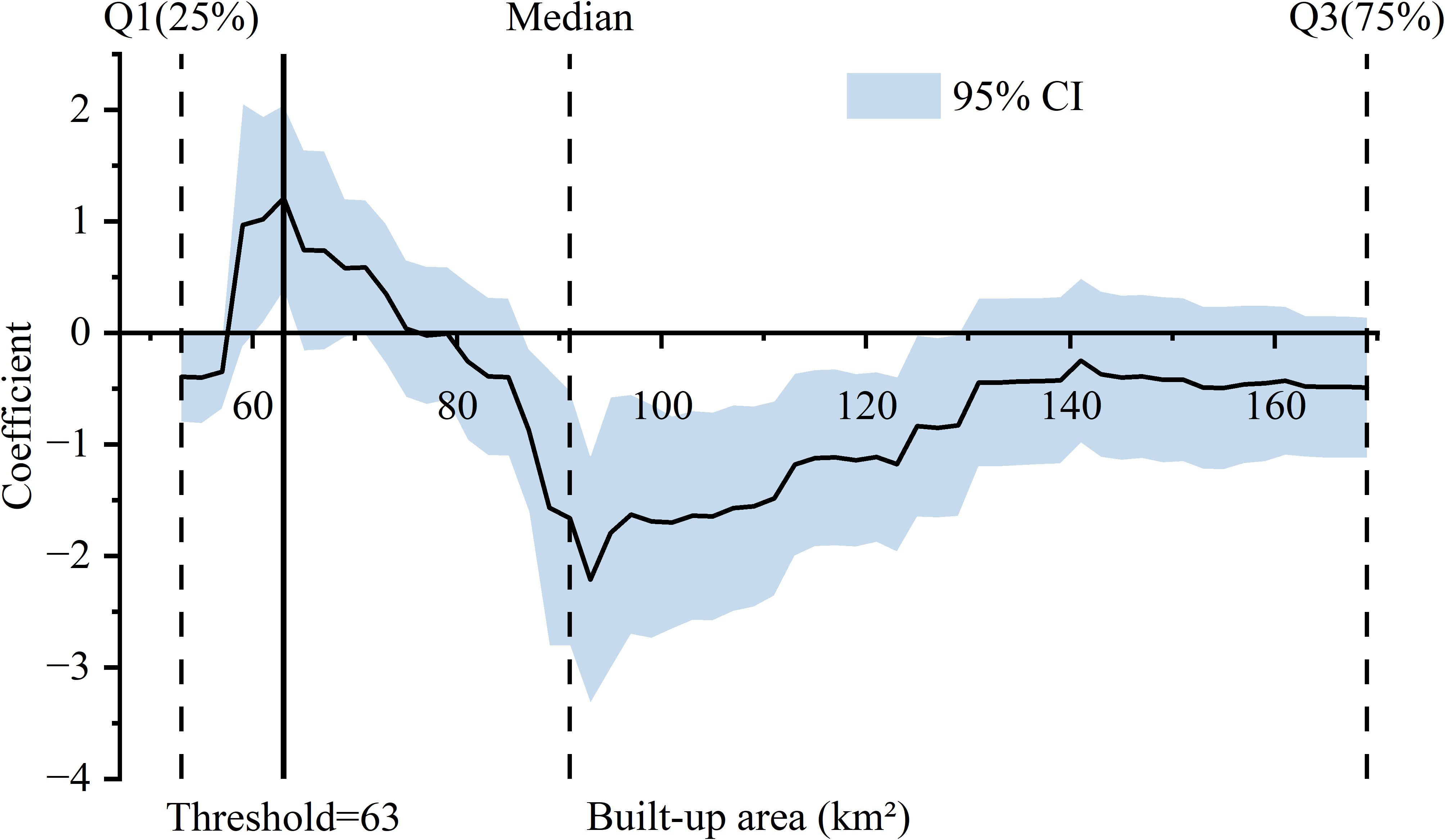
Figure 5. Threshold plot of the effect of built-up area.

Table 4 highlights a shift in the relationship between built-up area and MPA area. For built-up areas ≤63 km², both the time and built-up area variables are positively correlated with the dependent variable, with the built-up area coefficient being statistically significant (1.208 in Model 1, p<0.01), suggesting that increases in built-up area are associated with increases in the dependent variable. However, for built-up areas >63 km², the relationship changes, with the built-up area coefficient turning negative (-0.295 in Model 3 and -0.280 in Model 4, both p<0.001), indicating that as urbanization increases beyond this threshold, the dependent variable decreases. Building up 100 km² results in $1-{\text{e}}^{-0.280}=24.42\%$ or $1-{\text{e}}^{-0.295}=25.55\%$ decrease in MPA size.

Table 4

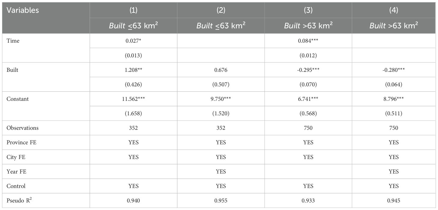
Table 4. Threshold regression results of the effect of built-up area.

3.3.3 Maritime traffic

Figure 6 illustrates the inverted N-shaped curve. Before this threshold at 0.33 million, the coefficient is insignificantly negative. After the threshold, the coefficient rises sharply, becoming significantly positive and stabilizing as maritime traffic increases beyond 0.33 million persons. Once maritime traffic exceeds the threshold, the positive relationship becomes more stable, suggesting a diminishing negative impact or a shift to a positive association with the dependent variable. This proves that maritime traffic is not necessarily antagonistic to MPA development.

Figure 6

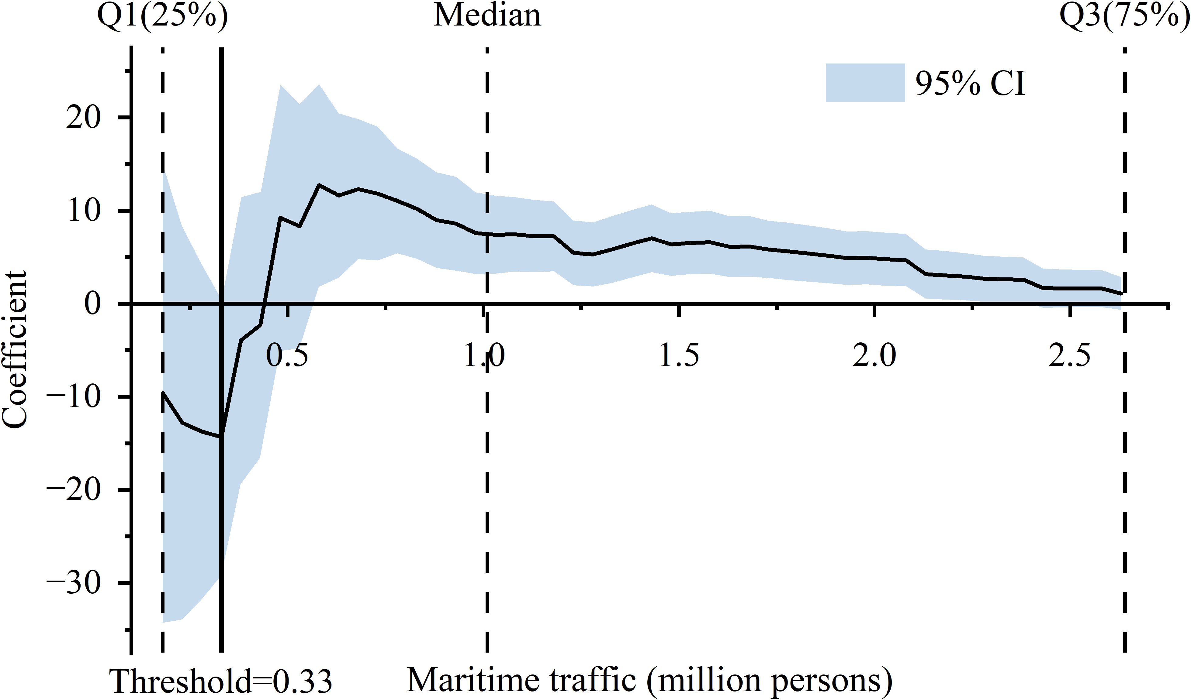
Figure 6. Threshold plot of the effect of maritime traffic.

Table 5 presents a threshold at 330,000 in the traffic variable. In Model 2 ($Traffic$ ≤330,000), the coefficient for traffic is negative and statistically significant (-26.362, p<0.001), indicating a strong negative relationship. After surpassing the threshold in Models 3 and 4 ($Traffic$ >330,000), the coefficient becomes significantly positive (0.502 and 0.472, p<0.01), showing a shift to a positive relationship. Averagely, 1 million more traffic is related to ${\text{e}}^{0.472\times 0.1}-1=4.83\%$ or ${\text{e}}^{0.502\times 0.1}-1=5.15\%$ increase in MPA size.

Table 5

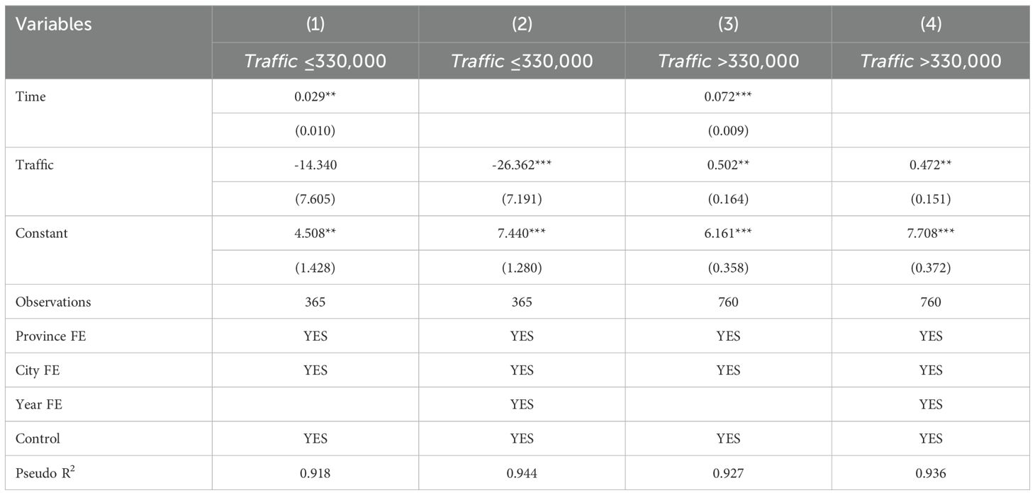
Table 5. Threshold regression results of the effect of maritime traffic.

4 Discussions

4.1 Theoretical contributions

4.1.1 Determinants of MPA establishment

Applying the SES theory, the study highlights the importance of spatial-ecological and socioeconomic factors in decision-making processes, thus contributing to the theoretical foundation of environmental governance and management. Although previous MPA studies did consider spatial scale as a factor (Fox et al., 2012; Fouqueray and Papyrakis, 2019; Yang and Wu, 2022), ecological capacity was unavailable due to data difficulty. This study demonstrates that conditions such as precipitation, wind speed, and green space also play a crucial role in shaping the richness and abundance of marine species and thus MPAs. Additionally, maritime traffic is not necessarily negative for MPA establishment. Further studies can use conclusions in this article to construct land-sea datasets despite ocean data scarcity.

4.1.2 Rethinking the EKC in MPAs

Results confirmed environmental Kuznets curves for GDP (N-shape), built-up area (N-shape) and maritime traffic (inverted N-shape) but offers some new insights. Although previous studies used quadratic terms (parabola) to fit the U-shaped EKC in MPA establishment (Fouqueray and Papyrakis, 2019; Mance et al., 2021; Bimonte and Stabile, 2024), including in China (Wang et al., 2025a), this article highlights the N-shaped (cubic) pattern. At the GDP threshold of ¥55 billion (1998-based), the coefficient initially drops slightly before gradually increasing and stabilizing, unlike the U-shaped expectation of a smooth, continuous shift toward environmental improvement (Tatoğlu and Polat, 2021). This behavior introduces a more refined understanding of the EKC, indicating that the shift toward environmental improvement may involve temporary setbacks before stabilization, pointing to the need for nuanced policy interventions during periods of economic transformation.

The N-shaped curve of marine conservation corresponds to the inverted N-shaped curve of environmental degradation, which often involves complex systems with multilateral interactions, feedback loops and regime shifts (Wu et al., 2022; Zhao et al., 2022; Warchold and Pradhan, 2025). This implies that linearizing and simplifying MPA establishment are insufficient. The economy, society and ecosystem should be considered complex adaptive systems intertwined in SES theories, including the original linked SES (Folke and Berkes, 1998), the Panarchy framework with connected adaptive cycles at different scales (Gunderson and Holling, 2002), the Telecoupling framework with coupled human and natural systems (Liu et al., 2016), common-pool resource institutional analysis (Ostrom, 2007; 2009), the robustness framework (Anderies et al., 2004), social-ecological action situation (SE-AS) (Schlüter et al., 2019) and socio-oceanography (Popova et al., 2023; Chen et al., 2024; Chen and Xu, 2024b).

4.1.3 Mathematically based threshold

This study also developed a PPMLHDFE threshold algorithm, which effectively enabled the discovery of the N-shaped GDP curve. Despite the excellence of PPMLHDFE to address overdispersion and heteroskedasticity, a threshold regression program was not universally applicable (Usman and Alola, 2023). Previously, PPMLHDFE was only able for robustness check, and the threshold calculation relies on other commands (Hansen, 1999; 2000). This article demonstrates that by controlling the three key mathematical conditions (local extremity, forward extremity and transcendentality), the algorithm could correctly find thresholds that ensure the significance of coefficients on both sides of the point.

4.2 Practical implications

4.2.1 Balance between conservation and development

According to CCSYs, in 1998, more than half (36) coastal cities were below the ¥55 billion (1998-based) threshold. In 2020, only 5 coastal cities are below the ¥106.5 billion (2020-based) threshold. This means most coastal cities have passed the first turning point of the N-shaped EKC. However, there are still 17 coastal cities below the second critical point of around ¥209.1 billion (2020-based). They are (in descending 2020 GDP): Rizhao, Haikou, Qinhuangdao, Zhoushan, Qinzhou, Yangjiang, Yingkou, Panjin, Beihai, Shanwei, Chaozhou, Jinzhou, Dandong, Huludao, Fangchenggang, Sanya and Danzhou. The cities relatively even out to south (10) and north (7). For these cities, the strife between development and conservation persists. This ongoing conflict emphasizes the need for targeted policies to foster both economic prosperity and environmental protection. In fact, many of these cities were approved for the Central Marine Ecological Protection and Restoration Fund since 2021 (Ma et al., 2022). This study delivers a data-driven argument in favor of sustained policy interventions for these cities.

4.2.2 Spatial-ecological and socioeconomic alignment

Multivariate results demonstrate that MPAs must be strategically planned and managed through the dual lens of spatial-ecological dynamics and socioeconomic realities. The study’s log-link model ($A={\text{e}}^{x\beta }$) reveals that MPA expansion exhibits percentage-based growth, where each contributing factor (e.g., GDP, infrastructure, green space) exerts proportional influence. This aligns with Liebig’s Law of the Minimum: MPA growth is constrained by the scarcest resource, not cumulative inputs. Cities experiencing diminishing marginal returns in GDP or infrastructure development could reallocate efforts toward ecological restoration or technological development to unlock MPA scalability. For instance, upgrading wastewater systems or restoring coastal habitats may yield greater marginal gains in MPA effectiveness than further industrial or urban expansion. As China turns to high-quality instead of GDP-oriented development (Pan et al., 2021), this study offers an empirically grounded framework to operationalize this paradigm shift in marine conservation. Altogether, these call for social-ecological fit (Chen and Xu, 2024a; Chen and Xu, 2024c) and top-down adaptive governance in China’s context, given its centralized governance structure.

4.2.3 Top-down adaptive governance

Judging from the city-level determinants of MPA establishment, marine adaptive governance works not only on the national level, but also operates locally. The implementation of adaptive governance in China’s MPAs necessitates a dynamic interplay between institutional rigidity and implementation flexibility within a centralized framework and three essential phases (Figure 7). In Phase 1 (active conservation), drawing upon the tenets of the SES theory, the central government (governance system) (Gao et al., 2024) is empowered to legislate, thereby delineating the governance framework. Meanwhile, the establishment of a hierarchical decision-making apparatus grants local governments (resource units) the latitude to effectuate necessary adjustments. Provincial governments are authorized to designate “adaptive management areas” outside national protected areas based on ecological threshold indicators such as coral reef coverage and fishery stock levels, dynamically adjusting the intensity of development. This “top-down design, local innovation” model ensures the authority of the national ecological strategy while responding to regional differences through data-driven, dynamic management and control.

Figure 7

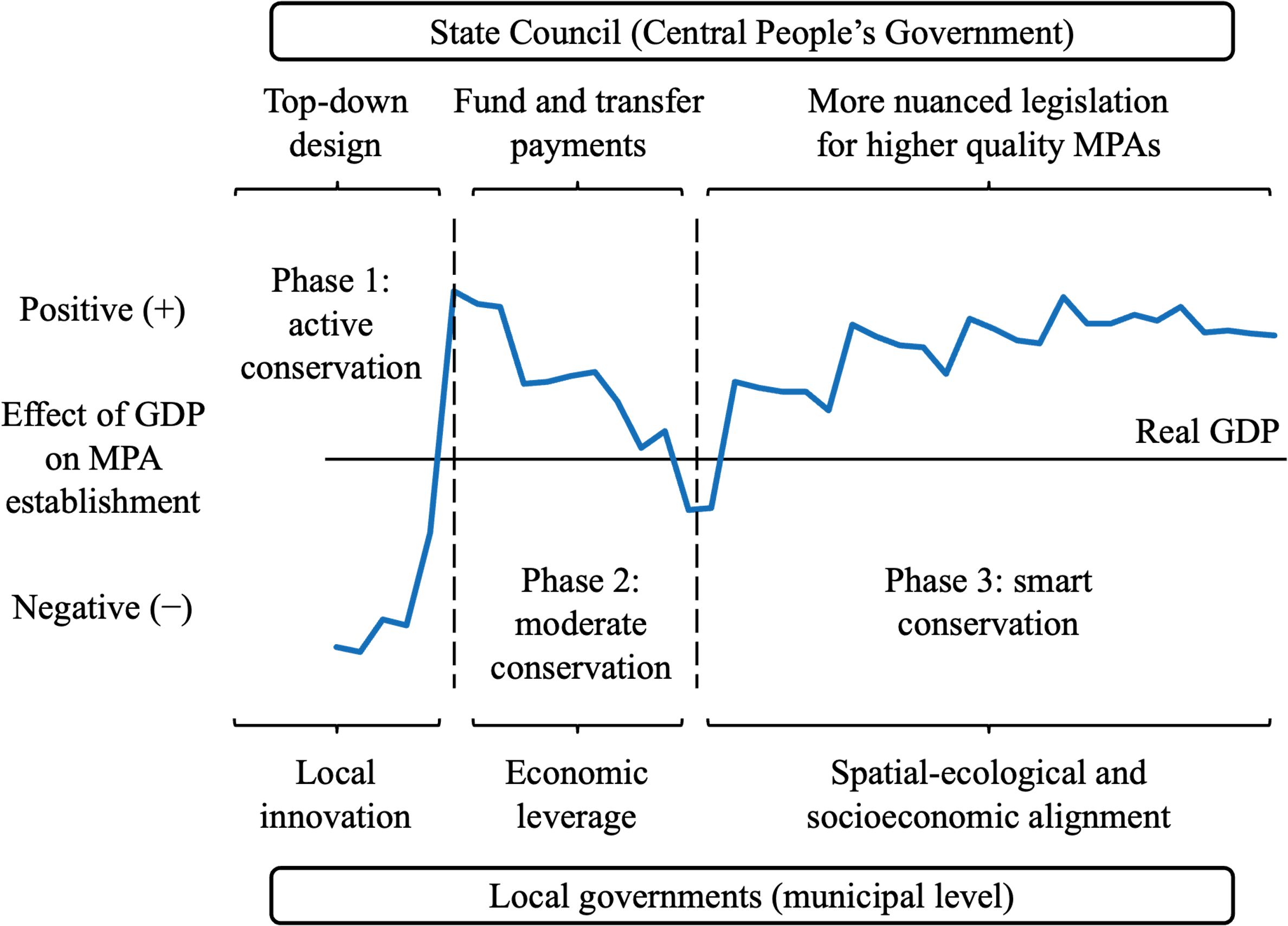
Figure 7. The top-down adaptive governance framework.

In Phase 2 (moderate conservation), the central government must incorporate ecological indicators, such as the MPA connectivity index and species recovery rate, into local performance assessments and establish direct links with fiscal transfer payments. Concurrently, innovative market instruments such as “blue carbon trading” should be developed to enable regions that have met ecological standards to convert the amount of carbon sequestered by mangroves into cross-regional trading quotas. This will encourage local governments to transition from passive compliance to active innovation and internalize the external costs of protected areas through economic leverage. The judicious integration of rigid constraints and flexible instruments is pivotal in operationalizing the principle of adaptive governance, persuading government departments to proactively arbitrate between the imperatives of conservation and development.

In Phase 3 (smart conservation), at the knowledge integration level, the establishment of a cross-scale information collaboration mechanism is imperative. By integrating multi-source data, such as satellite remote sensing, artificial intelligence monitoring, and community observations, and by opening hierarchical permissions to local governments, the deep integration of scientific models and traditional ecological knowledge can be promoted. The restructuring of the incentive system emerges as a pivotal institutional lever. These contribute to the enhancement of China’s “adaptive governance” approach, a contribution that is set to be disseminated globally for the enhancement of MPA management.

4.3 Limitations and future research

The study can be improved in data quality, spatiotemporal heterogeneity, and methodological rigor. First, the granularity of the spatial-ecological data should be refined, ideally upgrading to satellite images, long-term hydrological monitoring or oceanographic databases. Second, comparative studies across different regions would be suitable for China’s diverse coastlines. Finally, as the results indicate strong nonlinearity and complexity, future research should dive into complex system methods, such as hypergraph system dynamics to study the higher-order interactions of MPA establishment.

5 Conclusions

Adapting the SES approach, this article provides a comprehensive framework and analysis of the spatiotemporal distribution and determinants of China’s MPAs. The influencing factors are categorized into spatial-ecological capacity (natural conditions and land-sea space) and socioeconomic capacity (policy factors and economy size), corresponding to the resource-governance systems and units in the SES framework. Using overdispersion-robust PPML regressions with high-dimensional fixed effects and a mathematically based threshold algorithm, results reveal the thresholds are ¥55 billion (1998-based, equal to ¥106.5 billion in 2020) for GDP to be conducive to MPA establishment. Built-up areas over 63 km² are antagonistic to MPA development. It also suggests that urban green space can be helpful to MPA establishment, and that maritime traffic is not necessarily impeditive. Illustrated by an N-shaped curve, the article supplements previous studies of the U-shaped environmental Kuznets curve in MPA establishment, providing new theoretical insights from a complex system perspective. Drawing on the results, practical implications were given for balance between conservation and development, spatial-ecological and socioeconomic alignment and top-down adaptive governance. Future studies and international research can apply nonlinear conclusions in this study to deepen MPA establishment mechanisms with higher-order interactions and complex dynamics.

Data availability statement

The number and area of China’s MPAs are shared by Bohorquez et al. (2021) and can be found at https://datadryad.org/dataset/doi:10.5061/dryad.9zw3r22g2#. Precipitation and wind speed data from the Global Historical Climatology Network-hourly (GHCNh) at https://www.ncei.noaa.gov/metadata/geoportal/rest/metadata/item/gov.noaa.ncdc:C01688/html#. China City Statistical Yearbooks can be found from CNKI (China National Knowledge Infrastructure) at https://data.cnki.net. The compiled dataset, replicable Stata codes and descriptive statistics are stored at https://github.com/3220001030/MPA.

Author contributions

MC: Conceptualization, Data curation, Formal Analysis, Funding acquisition, Investigation, Methodology, Project administration, Resources, Software, Supervision, Validation, Visualization, Writing – original draft, Writing – review & editing. ZX: Data curation, Methodology, Resources, Software, Validation, Visualization, Writing – original draft, Writing – review & editing. YW: Data curation, Software, Validation, Visualization, Writing – original draft, Writing – review & editing.

Funding

The author(s) declare that financial support was received for the research and/or publication of this article. This research was funded by National Natural Science Foundation of China-Macao Science and Technology Development Fund (NSFC-FDCT) Joint Project, No.: (0011/2021/AFJ)4211101006, Southern Marine Science and Engineering Guangdong Laboratory (Zhuhai) 2020 Project, No. SML2020SP002. And this paper also funded by Team fund support of SML.

Acknowledgments

We thank the Marine Conservation and Integrated Governance Interdisciplinary Team (MCIGI) for their support and help and all the scholars for their help in the process of writing the paper. We also gratefully acknowledge the reviewers for their valuable time spent reviewing this paper.

Conflict of interest

The authors declare that the research was conducted in the absence of any commercial or financial relationship that could be construed as a potential conflict of interest.

Generative AI statement

The author(s) declare that no Generative AI was used in the creation of this manuscript.

Publisher’s note

All claims expressed in this article are solely those of the authors and do not necessarily represent those of their affiliated organizations, or those of the publisher, the editors and the reviewers. Any product that may be evaluated in this article, or claim that may be made by its manufacturer, is not guaranteed or endorsed by the publisher.

References

Acheampong A. O. and Opoku E. E. O. (2023). Environmental degradation and economic growth: Investigating linkages and potential pathways. Energ. Econ. 123, 106734. doi: 10.1016/j.eneco.2023.106734

Crossref Full Text | Google Scholar

Addas A. (2023). The importance of urban green spaces in the development of smart cities. Front. Environ. Sci. Volume 11. doi: 10.3389/fenvs.2023.1206372

Crossref Full Text | Google Scholar

Anderies J. M., Janssen M. A., and Ostrom E. (2004). A framework to analyze the robustness of social-ecological systems from an institutional perspective. Ecol. Soc 9 (1), 18. doi: 10.5751/ES-00610-090118

Crossref Full Text | Google Scholar

Andersson J., Lennerfors T. T., and Fornstedt H. (2024). Towards a socio-techno-ecological approach to sustainability transitions. Environ. Innov. Soc Transit. 51, 100846. doi: 10.1016/j.eist.2024.100846

Crossref Full Text | Google Scholar

Anderton C. H. and Anderton R. A. (2021). The trade disruption hypothesis fails for state-sponsored genocides and mass atrocities: why it matters. Peace Econ. Peace Sci. Public Policy 27, 143–168. doi: 10.1515/peps-2020-0060

Crossref Full Text | Google Scholar

Anti S. (2022). Investment treaties, local institutions and policies in the global land rush. World Bank Econ. Rev. 36, 559–582. doi: 10.1093/wber/lhac004

Crossref Full Text | Google Scholar

Appleton M. R., Courtiol A., Emerton L., Slade J. L., Tilker A., Warr L. C., et al. (2022). Protected area personnel and ranger numbers are insufficient to deliver global expectations. Nat. Sustain. 5, 1100–1110. doi: 10.1038/s41893-022-00970-0

Crossref Full Text | Google Scholar

Arai T. and Kimura S. (2024). Environmental factors influencing inshore migration in Japanese eel Anguilla japonica. Environ. Res. Commun. 6, 115037. doi: 10.1088/2515-7620/ad954a

Crossref Full Text | Google Scholar

Aregbesola A., Emmanuel O. S., and Adebisi T. (2024). Going to the cities: the strategic roles of public libraries in promoting sustainable development goals. Public Libr. Q. 43, 367–384. doi: 10.1080/01616846.2023.2253692

Crossref Full Text | Google Scholar

Arteaga M., Vásquez S. I., Neira S., and Cubillos L. (2024). Effect of wind variability on the recruitment of anchovy in the southern Humboldt upwelling ecosystem. Fish. Oceanogr. 33, e12677. doi: 10.1111/fog.12677

Crossref Full Text | Google Scholar

Bai P., Ling Z., Zhang S., Xie L., and Yang J. (2020). Fast-changing upwelling off the west coast of Hainan Island. Ocean Model. 148, 101589. doi: 10.1016/j.ocemod.2020.101589

Crossref Full Text | Google Scholar

Baier S. L. and Bergstrand J. H. (2007). Do free trade agreements actually increase members’ international trade? J. Int. Econ. 71, 72–95. doi: 10.1016/j.jinteco.2006.02.005

Crossref Full Text | Google Scholar

Balmford A., Gravestock P., Hockley N., McClean C. J., and Roberts C. M. (2004). The worldwide costs of marine protected areas. Proc. Natl. Acad. Sci. 101, 9694–9697. doi: 10.1073/pnas.0403239101

PubMed Abstract | Crossref Full Text | Google Scholar

Ban N. C., Evans L. S., Nenadovic M., and Schoon M. (2015). Interplay of multiple goods, ecosystem services, and property rights in large social-ecological marine protected areas. Ecol. Soc 20 (4), 2. doi: 10.5751/ES-07857-200402

Crossref Full Text | Google Scholar

Bareille F., Wolfersberger J., and Zavalloni M. (2023). Institutions and conservation: The case of protected areas. J. Environ. Econ. Manage. 118, 102768. doi: 10.1016/j.jeem.2022.102768

Crossref Full Text | Google Scholar

Bille R. A., Jensen K. E., and Buitenwerf R. (2023). Global patterns in urban green space are strongly linked to human development and population density. Urban For. Urban Green. 86, 127980. doi: 10.1016/j.ufug.2023.127980

Crossref Full Text | Google Scholar

Bimonte S. and Stabile A. (2024). Protected areas and the environmental kuznets curve in European countries. For. Policy Econ. 161, 103186. doi: 10.1016/j.forpol.2024.103186

Crossref Full Text | Google Scholar

Bohorquez J. J., Xue G., Frankstone T., Grima M. M., Kleinhaus K., Zhao Y., et al. (2021). China’s little-known efforts to protect its marine ecosystems safeguard some habitats but omit others. Sci. Adv. 7, eabj1569. doi: 10.1126/sciadv.abj1569

PubMed Abstract | Crossref Full Text | Google Scholar

Brander L. M., van Beukering P., Nijsten L., McVittie A., Baulcomb C., Eppink F. V., et al. (2020). The global costs and benefits of expanding Marine Protected Areas. Mar. Policy 116, 103953. doi: 10.1016/j.marpol.2020.103953

Crossref Full Text | Google Scholar

Bulleri F. and Chapman M. G. (2010). The introduction of coastal infrastructure as a driver of change in marine environments. J. Appl. Ecol. 47, 26–35. doi: 10.1111/j.1365-2664.2009.01751.x

Crossref Full Text | Google Scholar

Burkhalter J. C., Fefferman N. H., and Lockwood J. L. (2015). The impact of personality on the success of prospecting behavior in changing landscapes. Curr. Zool. 61, 557–568. doi: 10.1093/czoolo/61.3.557

Crossref Full Text | Google Scholar

Cao W., Zhou Y., Li R., Li X., and Zhang H. (2021). Monitoring long-term annual urban expansion, (1986–2017) in the largest archipelago of China. Sci. Total Environ. 776, 146015. doi: 10.1016/j.scitotenv.2021.146015

Crossref Full Text | Google Scholar

Checon H. H., Costa H. H. R., Corte G. N., Souza F. M., and Pombo M. (2023). Rainfall influences the patterns of diversity and species distribution in sandy beaches of the amazon coast. Sustainability 15, 5417. doi: 10.3390/su15065417

Crossref Full Text | Google Scholar

Chen M., Wang Y., and Xu Z. (2024). A framework for assessing the blue equity of social-ocean systems in marine governance transformation. Front. Mar. Sci. 11. doi: 10.3389/fmars.2024.1403194

Crossref Full Text | Google Scholar

Chen M. and Xu Z. (2024a). Assessing socio-ecological fit of international environmental agreements and trade-embodied carbon flows. Environ. Impact Assess. Rev. 106, 107534. doi: 10.1016/j.eiar.2024.107534

Crossref Full Text | Google Scholar

Chen M. and Xu Z. (2024b). A deep learning classification framework for research methods of marine protected area management. J. Environ. Manage. 368, 122228. doi: 10.1016/j.jenvman.2024.122228

PubMed Abstract | Crossref Full Text | Google Scholar

Chen M. and Xu Z. (2024c). Optimization of social-ecological fit in China’s Sousa Chinensis protected areas based on modified Moran’s I. Ocean Coast. Manage. 255, 107234. doi: 10.1016/j.ocecoaman.2024.107234

Crossref Full Text | Google Scholar

Chen M. and Xu Z. (2024d). Visualising Sustainable Development Goals progress of China’s coastal cities using circular-kaleidoscope charts. Reg. Stud. Reg. Sci. 11, 474–478. doi: 10.1080/21681376.2024.2374403

Crossref Full Text | Google Scholar

Chen M., Xu Z., and Wang Y. (2023). Entry barriers and tripartite evolutionary game analysis of seawater desalination under the government regulation in China. Front. Mar. Sci. 10. doi: 10.3389/fmars.2023.1309515

Crossref Full Text | Google Scholar

Choi K.-R., Kim J.-H., and Yoo S.-H. (2020). Public perspective on constructing sea forests as a public good: A contingent valuation experiment in South Korea. Mar. Policy 120, 104146. doi: 10.1016/j.marpol.2020.104146

Crossref Full Text | Google Scholar

Cigarini A., Bonhoure I., Vicens J., and Perelló J. (2021). Public libraries embrace citizen science: Strengths and challenges. Libr. Inf. Sci. Res. 43, 101090. doi: 10.1016/j.lisr.2021.101090

Crossref Full Text | Google Scholar

Correia S. (2015). Singletons, cluster-robust standard errors and fixed effects: A bad mix. Available online at: https://scorreia.com/research/singletons.pdf (Accessed April 16, 2025).

Google Scholar

Correia S., Guimarães P., and Zylkin T. (2020). Fast Poisson estimation with high-dimensional fixed effects. Stata J. 20, 95–115. doi: 10.1177/1536867x20909691

Crossref Full Text | Google Scholar

Correia S., Guimarães P., and Zylkin T. (2021). Verifying the existence of maximum likelihood estimates for generalized linear models. Available online at: http://arxiv.org/abs/1903.01633 (Accessed April 16, 2025).

Google Scholar

Curzi D. and Huysmans M. (2022). The impact of protecting EU geographical indications in trade agreements. Am. J. Agric. Econ. 104, 364–384. doi: 10.1111/ajae.12226

Crossref Full Text | Google Scholar

da Silva V. E. L., Dolbeth M., and Fabré N. N. (2021). Assessing tropical coastal dynamics across habitats and seasons through different dimensions of fish diversity. Mar. Environ. Res. 171, 105458. doi: 10.1016/j.marenvres.2021.105458

PubMed Abstract | Crossref Full Text | Google Scholar

Davies B. F. R., Holmes L., Bicknell A., Attrill M. J., and Sheehan E. V. (2022). A decade implementing ecosystem approach to fisheries management improves diversity of taxa and traits within a marine protected area in the UK. Divers. Distrib. 28, 173–188. doi: 10.1111/ddi.13451

Crossref Full Text | Google Scholar

Devine J. and Appleton L. (2023). Environmental education in public libraries. Libr. Manage. 44, 152–165. doi: 10.1108/LM-10-2022-0091

Crossref Full Text | Google Scholar

Ding Y., Matta M., Gopal R. D., and Xu H. (2025). Ruckus in the rentals, seeking new arrangements: remedying the impact of home-sharing on urban noise. Manage. Inf. Syst. Q. 49, 389–408. doi: 10.25300/MISQ/2024/18049

Crossref Full Text | Google Scholar

Dong S., Ren G., Xue Y., and Liu K. (2023a). Urban green innovation’s spatial association networks in China and their mechanisms. Sustain. Cities Soc 93, 104536. doi: 10.1016/j.scs.2023.104536

Crossref Full Text | Google Scholar

Dong S., Xue Y., Ren G., and Liu K. (2023b). Urban green innovation efficiency in China: spatiotemporal evolution and influencing factors. Land 12, 75. doi: 10.3390/land12010075

Crossref Full Text | Google Scholar

Ekanayake P. N. S. P., Madsen J. B., and Bharati T. (2023). Trade and economic growth: Does the sophistication of traded goods matter? J. Econ. Growth 28, 481–524. doi: 10.1007/s10887-023-09224-w

Crossref Full Text | Google Scholar

Espinoza M., Quesada-Perez F., Madrigal-Mora S., Naranjo-Elizondo B., Clarke T. M., and Cortés J. (2024). A decade of submersible observations revealed temporal trends in elasmobranchs in a remote island of the Eastern Tropical Pacific Ocean. Sci. Rep. 14, 13786. doi: 10.1038/s41598-024-64157-7

PubMed Abstract | Crossref Full Text | Google Scholar

Fávero L. P. L., Belfiore P., Santos M., and Souza R. F. (2020). Overdisp: A stata (and mata) package for direct detection of overdispersion in poisson and negative binomial regression models. Stat. Optim. Inf. Comput. 8 (3), 773–789. doi: 10.19139/soic-2310-5070-557

Crossref Full Text | Google Scholar

Folke C. and Berkes F. (1998). “Understanding dynamics of ecosystem-institution linkages for building resilience,” in Beijer discussion paper no. 112 (The Beijer Institute of Ecological Economics, The Royal Swedish Academy of Sciences, Stockholm, Sweden). Available at: https://beijer.kva.se/wp-content/uploads/2019/10/7238862_disc112artikel.pdf (Accessed April 14, 2025).

Google Scholar

Food and Agriculture Organization (2024). Regulations of the people’s republic of China on nature reserves. Available online at: https://www.fao.org/faolex/results/details/en/c/LEX-FAOC011954/ (Accessed April 14, 2025).

Google Scholar

Fouqueray M. and Papyrakis E. (2019). An empirical analysis of the cross-national determinants of marine protected areas. Mar. Policy 99, 87–93. doi: 10.1016/j.marpol.2018.10.017

Crossref Full Text | Google Scholar

Fox H. E., Soltanoff C. S., Mascia M. B., Haisfield K. M., Lombana A. V., Pyke C. R., et al. (2012). Explaining global patterns and trends in marine protected area (MPA) development. Mar. Policy 36, 1131–1138. doi: 10.1016/j.marpol.2012.02.007

Crossref Full Text | Google Scholar

Friedmann J.-C. and Pedersen T. (2024). National innovation policies and knowledge acquisition in international alliances. Glob. Strategy J. 14, 116–151. doi: 10.1002/gsj.1477

Crossref Full Text | Google Scholar

Fuente B., Bertzky B., Delli G., Mandrici A., Conti M., Florczyk A. J., et al. (2020). Built-up areas within and around protected areas: Global patterns and 40-year trends. Glob. Ecol. Conserv. 24, e01291. doi: 10.1016/j.gecco.2020.e01291

PubMed Abstract | Crossref Full Text | Google Scholar

Gao C., Xia S., Liu J., Tao H., and Zhu Z. (2024). Adaptive evolution and dynamic mechanism of resort socioecological system in tourism cities: The case of Qinhuangdao, China. Habitat Int. 151, 103138. doi: 10.1016/j.habitatint.2024.103138

Crossref Full Text | Google Scholar

Geng Q. and Lo K. (2024). Geopolitical strategies and transnational environmental governance: A comparative study of international NGOs in Cambodia. Geoforum 154, 104063. doi: 10.1016/j.geoforum.2024.104063

Crossref Full Text | Google Scholar

Giang P. Q. and Khanal R. (2024). What next for marine ecosystem management in Vietnam: assessment of coastal economy, climate change, and policy implication. Environ. Res. Commun. 6, 025002. doi: 10.1088/2515-7620/ad19a5

Crossref Full Text | Google Scholar

Giorgi J., Plunket A., and Starosta de Waldemar F. (2025). Inter-regional highly skilled worker mobility and technological novelty. Res. Policy 54, 105113. doi: 10.1016/j.respol.2024.105113

Crossref Full Text | Google Scholar

Go Y.-H., Lau L.-S., Liew F.-M., and Senadjki A. (2021). A transport environmental Kuznets curve analysis for Malaysia: exploring the role of corruption. Environ. Sci. Pollut. Res. 28, 3421–3433. doi: 10.1007/s11356-020-10736-w

PubMed Abstract | Crossref Full Text | Google Scholar

Gong M., Teller N., Golebie E. J., Aczel M., Jiang Z., Van Zeghbroeck J., et al. (2024). Unveiling complementarities between mangrove restoration and global sustainable development goals. J. Clean. Prod. 474, 143524. doi: 10.1016/j.jclepro.2024.143524

Crossref Full Text | Google Scholar

Gu H., Jianfa S., and Chu J. (2023). Understanding intercity mobility patterns in rapidly urbanizing China 2015–2019: evidence from longitudinal poisson gravity modeling. Ann. Am. Assoc. Geogr. 113, 307–330. doi: 10.1080/24694452.2022.2097050

Crossref Full Text | Google Scholar

Gu H., Jie Y., and Lao X. (2022). Health service disparity, push-pull effect, and elderly migration in ageing China. Habitat Int. 125, 102581. doi: 10.1016/j.habitatint.2022.102581

Crossref Full Text | Google Scholar

Gu H., Wang J., and Ling Y. (2024). Economic geography of talent migration and agglomeration in China: A dual-driver framework. China Econ. Rev. 86, 102180. doi: 10.1016/j.chieco.2024.102180

Crossref Full Text | Google Scholar

Gu H. and Xu Z. (2022). Kaleidoscope visualisation of China’s internal migration 1985–2020. Environ. Plan. B: Urban Anal. City Sci. 49, 1341–1344. doi: 10.1177/23998083221082916

Crossref Full Text | Google Scholar

Gu H., Xu Z., Zheng J., and Shen T. (2022b). Visualising global currents of international students between 1999 and 2018. Environ. Plan. A 54, 3–6. doi: 10.1177/0308518x211055180

Crossref Full Text | Google Scholar

Gunderson L. H. and Holling C. S. (2002). Panarchy: understanding transformations in human and natural systems (Washington, USA: Island Press). Available at: https://islandpress.org/books/panarchy#desc (Accessed April 14, 2025).

Google Scholar

Hansen B. E. (1999). Threshold effects in non-dynamic panels: Estimation, testing, and inference. J. Econom. 93, 345–368. doi: 10.1016/S0304-4076(99)00025-1

Crossref Full Text | Google Scholar

Hansen B. E. (2000). Sample splitting and threshold estimation. Econometrica 68, 575–603. doi: 10.1111/1468-0262.00124

Crossref Full Text | Google Scholar

Hao K., Han L., and Li W. (2022). The impact of China’s currency swap lines on bilateral trade. Int. Rev. Econ. Finance 81, 173–183. doi: 10.1016/j.iref.2022.05.004

Crossref Full Text | Google Scholar

He M. and Cliquet A. (2020). Challenges for protected areas management in China. Sustainability 12, 5879. doi: 10.3390/su12155879

Crossref Full Text | Google Scholar

Head K. and Mayer T. (2014). “Chapter 3 - Gravity Equations: Workhorse,Toolkit, and Cookbook,” in Handbook of International Economics. Eds. Gopinath G., Helpman E., and Rogoff K. (Amsterdam: Elsevier), 131–195. doi: 10.1016/B978-0-444-54314-1.00003-3

Crossref Full Text | Google Scholar

Heit D. R., Ortiz-Calo W., Poisson M. K. P., Butler A. R., and Moll R. J. (2024). Generalized nonlinearity in animal ecology: Research, review, and recommendations. Ecol. Evol. 14, e11387. doi: 10.1002/ece3.11387

PubMed Abstract | Crossref Full Text | Google Scholar

Hendrickx J. (2004). “COLDIAG2: Stata module to evaluate collinearity in linear regression,” in Statistical Software Components S445202 (Boston College Department of Economics). Available at: https://ideas.repec.org/c/boc/bocode/s445202.html (Accessed April 14, 2025).

Google Scholar

Herald T. E. and Ramirez-Marquez J. E. (2012). System element obsolescence replacement optimization via life cycle cost forecasting. IEEE Trans. Compon. Packag. Manuf. Technol. 2, 1394–1401. doi: 10.1109/TCPMT.2012.2201218

Crossref Full Text | Google Scholar

Hoeksema B. W., van der Loos L. M., and van Moorsel G. W. N. M. (2022). Coral diversity matches marine park zonation but not economic value of coral reef sites at St. Eustatius, eastern Caribbean. J. Environ. Manage. 320, 115829. doi: 10.1016/j.jenvman.2022.115829

PubMed Abstract | Crossref Full Text | Google Scholar

Hofstede G. (2011). Dimensionalizing cultures: The Hofstede model in context. Psychol. Cul. 2, 8. doi: 10.9707/2307-0919.1014

Crossref Full Text | Google Scholar

Horowitz J. K. (2002). Preferences in the future. Environ. Resour. Econ. 21, 241–258. doi: 10.1023/A:1014592629514

Crossref Full Text | Google Scholar

Hu W., Liu J., Ma Z., Wang Y., Zhang D., Yu W., et al. (2020). China’s marine protected area system: Evolution, challenges, and new prospects. Mar. Policy 115, 103780. doi: 10.1016/j.marpol.2019.103780

Crossref Full Text | Google Scholar

Jaffé R., Paul-Gorsline C., McDermott M., Fluharty S., Al-Shaikh I., Skeat S. L., et al. (2025). Using habitat suitability modeling to integrate ecosystem-based approaches for mangrove restoration site selection. Ecosphere 16, e70222. doi: 10.1002/ecs2.70222

Crossref Full Text | Google Scholar

Jaravel X. L. and Sager E. (2019). “What are the price effects of trade? Evidence from the US and implications for quantitative trade models,” in CEP Discussion Paper No 1642 (Centre for Economic Performance, London School of Economics and Political Science) (Washington: Board of Governors of the Federal Reserve System). doi: 10.17016/feds.2019.068

Crossref Full Text | Google Scholar

Jenkins L. D. (2022). Power, politics, and culture of marine conservation technology in fisheries. Conserv. Biol. 36, e13855. doi: 10.1111/cobi.13855

PubMed Abstract | Crossref Full Text | Google Scholar

Jiang W. and Jiang S. (2023). Evolution of regulations controlling human pressure in protected areas of China. Sustainability 15, 4469. doi: 10.3390/su15054469

Crossref Full Text | Google Scholar

Kalaycı S. and Özden C. (2021). The linkage among sea transport, trade liberalization and industrial development in the context of CO2: an empirical investigation from China. Front. Environ. Sci. Volume 9. doi: 10.3389/fenvs.2021.633875

Crossref Full Text | Google Scholar

Kirwan M. L. and Megonigal J. P. (2013). Tidal wetland stability in the face of human impacts and sea-level rise. Nature 504, 53–60. doi: 10.1038/nature12856

PubMed Abstract | Crossref Full Text | Google Scholar

Ko J.-H., Akeyoshi M., and Yoo D. (2022). The geography of gravity. Asia-Pac. J. Account. Econ. 29, 1560–1578. doi: 10.1080/16081625.2020.1730920

Crossref Full Text | Google Scholar

Kunofiwa T. (2022). Examining the determinants of foreign direct investment in BRICS. J. Account. Finance Emerg. Econ. 8 (2), 319–330. doi: 10.26710/jafee.v8i2.2353

Crossref Full Text | Google Scholar

Lansu E. M., Reijers V. C., Höfer S., Luijendijk A., Rietkerk M., Wassen M. J., et al. (2024). A global analysis of how human infrastructure squeezes sandy coasts. Nat. Commun. 15, 432. doi: 10.1038/s41467-023-44659-0

PubMed Abstract | Crossref Full Text | Google Scholar

Lapointe M., Rochman C. M., and Tufenkji N. (2022). Sustainable strategies to treat urban runoff needed. Nat. Sustain. 5, 366–369. doi: 10.1038/s41893-022-00853-4

Crossref Full Text | Google Scholar

Lay J. and Nolte K. (2017). Determinants of foreign land acquisitions in low- and middle-income countries. J. Econ. Geogr. 18, 59–86. doi: 10.1093/jeg/lbx011

Crossref Full Text | Google Scholar

Leszczensky L. and Wolbring T. (2022). How to deal with reverse causality using panel data? Recommendations for researchers based on a simulation study. Sociol. Methods Res. 51, 837–865. doi: 10.1177/0049124119882473

Crossref Full Text | Google Scholar

Li E., Ma Y., Wang Y., Chen Y., and Niu B. (2022). Competition among cities for export trade brings diversification: The experience of China’s urban export trade development. PloS One 17, e0271239. doi: 10.1371/journal.pone.0271239

PubMed Abstract | Crossref Full Text | Google Scholar

Li Y., Svenning J.-C., Zhou W., Zhu K., Abrams J. F., Lenton T. M., et al. (2024b). Green spaces provide substantial but unequal urban cooling globally. Nat. Commun. 15, 7108. doi: 10.1038/s41467-024-51355-0

PubMed Abstract | Crossref Full Text | Google Scholar

Li C., Zhang L., Chen S., Zhang T., Zhou J., He J., et al. (2024a). Has the Maritime Silk Road Initiative promoted the development and expansion of port city clusters along its route? Cities 151, 105127. doi: 10.1016/j.cities.2024.105127

Crossref Full Text | Google Scholar

Liu J., Yang W., and Li S. (2016). Framing ecosystem services in the telecoupled Anthropocene. Front. Ecol. Environ. 14, 27–36. doi: 10.1002/16-0188.1

Crossref Full Text | Google Scholar

Liu S., Zuo J., Shu Y., Ji Q., Cai Y., and Yao J. (2023). The intensified trend of coastal upwelling in the South China Sea during 1982-2020. Front. Mar. Sci. Volume 10. doi: 10.3389/fmars.2023.1084189

Crossref Full Text | Google Scholar

Long W., Zhoufu Y., and Markus L. (2025). Capital market integration and firm innovation: theory and evidence from China. Appl. Econ. 57, 956–974. doi: 10.1080/00036846.2024.2311057

Crossref Full Text | Google Scholar

Lu C., Goeman J., and Putter H. (2022). Maximum likelihood estimation in the additive hazards model. Biometrics 79, 1646–1656. doi: 10.1111/biom.13764

PubMed Abstract | Crossref Full Text | Google Scholar

Luo Y., Shi J., Guo X., Mao X., Yao P., Zhao B., et al. (2023). Yearly variations in nutrient supply in the East China sea due to the Zhejiang coastal upwelling and Kuroshio intrusion. J. Geophys. Res.: Oceans 128, e2022JC019216. doi: 10.1029/2022JC019216

Crossref Full Text | Google Scholar

Ma K. (2016). On key issues and possible solutions related to nature reserve management in China. Biodiv. Sci. 24, 249–251. doi: 10.17520/biods.2016082

Crossref Full Text | Google Scholar

Ma Z., Chen Y., Melville D. S., Fan J., Liu J., Dong J., et al. (2019). Changes in area and number of nature reserves in China. Conserv. Biol. 33, 1066–1075. doi: 10.1111/cobi.13285

PubMed Abstract | Crossref Full Text | Google Scholar

Ma W., Hoppe T., and de Jong M. (2022). Policy accumulation in China: A longitudinal analysis of circular economy initiatives. Sustain. Prod. Consum. 34, 490–504. doi: 10.1016/j.spc.2022.10.010

Crossref Full Text | Google Scholar

Macedo M. M., Angelini R., da Silva V. L., and Fabré N. N. (2021). Trophic structure of coastal meta-ecosystems in the tropical Southwestern Atlantic. Estuar. Coast. Shelf Sci. 263, 107654. doi: 10.1016/j.ecss.2021.107654

Crossref Full Text | Google Scholar

Macedo M., Fabré N. N., da Silva V. E. L., Santos M. E. F., Albuquerque-Tenório M. D., and Angelini R. (2023). Influence of the river flow pulse on the maturity, resilience, and sustainability of tropical coastal ecosystems. Mar. Environ. Res. 183, 105806. doi: 10.1016/j.marenvres.2022.105806

PubMed Abstract | Crossref Full Text | Google Scholar

MacKinnon K., van Ham C., Reilly K., and Hopkins J. (2019). “Nature-Based Solutions and Protected Areas to Improve Urban Biodiversity and Health,” in Biodiversity and Health in the Face of Climate Change. Eds. Marselle M. R., Stadler J., Korn H., Irvine K. N., and Bonn A. (Cham: Springer International Publishing), 363–380. doi: 10.1007/978-3-030-02318-8_16

Crossref Full Text | Google Scholar

Mance D., Krunić K., and Mance D. (2021). Protecting species by promoting protected areas and human development—A panel analysis. Sustainability 13, 11970. doi: 10.3390/su132111970

Crossref Full Text | Google Scholar

Mascia M. B., Fox H. E., Glew L., Ahmadia G. N., Agrawal A., Barnes M., et al. (2017). A novel framework for analyzing conservation impacts: evaluation, theory, and marine protected areas. Ann. N. Y. Acad. Sci. 1399, 93–115. doi: 10.1111/nyas.13428

PubMed Abstract | Crossref Full Text | Google Scholar

Matthews T. J., Rigal F., Triantis K. A., and Whittaker R. J. (2019). A global model of island species–area relationships. Proc. Natl. Acad. Sci. 116, 12337–12342. doi: 10.1073/pnas.1818190116

PubMed Abstract | Crossref Full Text | Google Scholar

McDermott A. (2021). Inner Workings: Reeling in answers to the “freshwater fish paradox. Proc. Natl. Acad. Sci. 118, e2113780118. doi: 10.1073/pnas.2113780118

PubMed Abstract | Crossref Full Text | Google Scholar

Moore-Maley B. and Allen S. E. (2022). Wind-driven upwelling and surface nutrient delivery in a semi-enclosed coastal sea. Ocean Sci. 18, 143–167. doi: 10.5194/os-18-143-2022

Crossref Full Text | Google Scholar

Mumelaš D. and Martek A. (2024). Benefits of citizen science for libraries. Publications 12, 8. doi: 10.3390/publications12010008

Crossref Full Text | Google Scholar

National Centers for Environmental Information (NCEI) (2023). Global historical climatology network-hourly (GHCNh). Available online at: https://www.ncei.noaa.gov/metadata/geoportal/rest/metadata/item/gov.noaa.ncdc:C01688/html (Accessed April 14, 2025).

Google Scholar

Nordio G. and Fagherazzi S. (2022). Salinity increases with water table elevation at the boundary between salt marsh and forest. J. Hydrol. 608, 127576. doi: 10.1016/j.jhydrol.2022.127576

Crossref Full Text | Google Scholar

Opršal Z., Harmáček J., Pavlík P., and Machar I. (2018). What Factors can Influence the Expansion of Protected Areas around the World in the Context of International Environmental and Development Goals? Probl. Ekorozwoju 13, 145–157. Available at: https://ph.pollub.pl/index.php/preko/article/download/5047/3937 (Accessed April 14, 2025).

Google Scholar

Ostrom E. (1990). Governing the commons: The evolution of institutions for collective action (Cambridge: Cambridge University Press). doi: 10.1017/CBO9780511807763

Crossref Full Text | Google Scholar

Ostrom E. (2007). A diagnostic approach for going beyond panaceas. Proc. Natl. Acad. Sci. 104, 15181–15187. doi: 10.1073/pnas.0702288104

PubMed Abstract | Crossref Full Text | Google Scholar

Ostrom E. (2009). A general framework for analyzing sustainability of social-ecological systems. Science 325, 419–422. doi: 10.1126/science.1172133

PubMed Abstract | Crossref Full Text | Google Scholar

Ostrom E. (2010a). Beyond markets and states: polycentric governance of complex economic systems. Am. Econ. Rev. 100, 641–672. doi: 10.1257/aer.100.3.641

Crossref Full Text | Google Scholar

Ostrom E. (2010b). Polycentric systems for coping with collective action and global environmental change. Glob. Environ. Change 20, 550–557. doi: 10.1016/j.gloenvcha.2010.07.004

Crossref Full Text | Google Scholar

Pan W., Wang J., Lu Z., Liu Y., and Li Y. (2021). High-quality development in China: Measurement system, spatial pattern, and improvement paths. Habitat Int. 118, 102458. doi: 10.1016/j.habitatint.2021.102458

Crossref Full Text | Google Scholar

Passos C. V. B., Fabré N. N., Malhado A. C. M., Batista V. S., and Ladle R. J. (2016). Estuarization increases functional diversity of demersal fish assemblages in tropical coastal ecosystems. J. Fish Biol. 89, 847–862. doi: 10.1111/jfb.13029

PubMed Abstract | Crossref Full Text | Google Scholar

Pata U. K., Ahmed Z., Eryilmaz S., Zeren F., and Gencer Y. G. (2023). Analyzing the environmental Kuznets curve for transportation modes in European countries. Transp. Res. D: Transp. Environ. 122, 103893. doi: 10.1016/j.trd.2023.103893

Crossref Full Text | Google Scholar

Peiró-Palomino J., Rodríguez-Crespo E., and Suárez-Varela M. (2022). Do countries with higher institutional quality transition to cleaner trade? Ecol. Econ. 201, 107554. doi: 10.1016/j.ecolecon.2022.107554

Crossref Full Text | Google Scholar

Phaka F. M., Vanhove M. P. M., du Preez L. H., and Hugé J. (2023). Library books as environmental management capacity building opportunities exclude most South African languages. Environ. Sci. Policy 141, 61–68. doi: 10.1016/j.envsci.2022.12.020

Crossref Full Text | Google Scholar

Pinheiro R. P., Akamatsu F. E., Macaya D. M., Itezerote A. M., Saleh S. O., Hojaij F., et al. (2022). Innervation of gluteus medius muscle and its relationship with myofascial pain. FASEB J. 36 (S1). doi: 10.1096/fasebj.2022.36.S1.L7710

Crossref Full Text | Google Scholar

Pinto L. V., Inácio M., and Pereira P. (2023). Green and blue infrastructure (GBI) and urban nature-based solutions (NbS) contribution to human and ecological well-being and health. Oxf. Open Infrastruct. Health 1 (2023), ouad004. doi: 10.1093/ooih/ouad004

Crossref Full Text | Google Scholar

Podda C. and Porporato E. M. D. (2023). Marine spatial planning for connectivity and conservation through ecological corridors between marine protected areas and other effective area-based conservation measures. Front. Mar. Sci. 10. doi: 10.3389/fmars.2023.1271397

Crossref Full Text | Google Scholar

Popova E., Aksenov Y., Amoudry L. O., Becker A., Bricheno L., Brown J. M., et al. (2023). Socio-oceanography: an opportunity to integrate marine social and natural sciences. Front. Mar. Sci. 10. doi: 10.3389/fmars.2023.1209356

Crossref Full Text | Google Scholar

Raimondi V. and Scoppola M. (2022). Foreign land acquisitions and environmental regulations: Does the pollution-haven effect hold? J. Agr. Econ. 73, 172–194. doi: 10.1111/1477-9552.12441

Crossref Full Text | Google Scholar

Roberts J. M., Devey C. W., Biastoch A., Carreiro-Silva M., Dohna T., Dorschel B., et al. (2023). A blueprint for integrating scientific approaches and international communities to assess basin-wide ocean ecosystem status. Commun. Earth Environ. 4, 12. doi: 10.1038/s43247-022-00645-w

Crossref Full Text | Google Scholar

Romañach S. S., DeAngelis D. L., Koh H. L., Li Y., Teh S. Y., Raja Barizan R. S., et al. (2018). Conservation and restoration of mangroves: Global status, perspectives, and prognosis. Ocean Coast. Manage. 154, 72–82. doi: 10.1016/j.ocecoaman.2018.01.009

Crossref Full Text | Google Scholar

Santos Silva J. M. C. and Tenreyro S. (2006). The log of gravity. Rev. Econ. Stat. 88, 641–658. doi: 10.1162/rest.88.4.641

Crossref Full Text | Google Scholar

Santos Silva J. M. C. and Tenreyro S. (2011). Further simulation evidence on the performance of the Poisson pseudo-maximum likelihood estimator. Econ. Lett. 112, 220–222. doi: 10.1016/j.econlet.2011.05.008

Crossref Full Text | Google Scholar

Santos Silva J. M. C. and Tenreyro S. (2022). The log of gravity at 15. Port. Econ. J. 21, 423–437. doi: 10.1007/s10258-021-00203-w

Crossref Full Text | Google Scholar

Saussay A. and Sato M. (2024). The impact of energy prices on industrial investment location: Evidence from global firm level data. J. Environ. Econ. Manage. 127, 102992. doi: 10.1016/j.jeem.2024.102992

Crossref Full Text | Google Scholar

Schilling H. T., Hinchliffe C., Gillson J. P., Miskiewicz A. G., and Suthers I. M. (2022). Coastal winds and larval fish abundance indicate a recruitment mechanism for southeast Australian estuarine fisheries. Fish. Oceanogr. 31, 40–55. doi: 10.1111/fog.12561

Crossref Full Text | Google Scholar

Schlüter M., Haider L. J., Lade S. J., Lindkvist E., Martin R., Orach K., et al. (2019). Capturing emergent phenomena in social-ecological systems. Ecol. Soc 24 (3), 11. doi: 10.5751/ES-11012-240311

Crossref Full Text | Google Scholar

Sims K. R. E. (2010). Conservation and development: Evidence from Thai protected areas. J. Environ. Econ. Manage. 60, 94–114. doi: 10.1016/j.jeem.2010.05.003

Crossref Full Text | Google Scholar

Smart L. S., Vukomanovic J., Sills E. O., and Sanchez G. (2021). Cultural ecosystem services caught in a ‘coastal squeeze’ between sea level rise and urban expansion. Glob. Environ. Change 66, 102209. doi: 10.1016/j.gloenvcha.2020.102209

Crossref Full Text | Google Scholar

Šmejkal M., Bartoň D., Blabolil P., Kolařík T., Kubečka J., Sajdlová Z., et al. (2023). Diverse environmental cues drive the size of reproductive aggregation in a rheophilic fish. Mov. Ecol. 11, 16. doi: 10.1186/s40462-023-00379-0

PubMed Abstract | Crossref Full Text | Google Scholar

Song B. (2021). “CNGDF: Stata module to calculate any base period GDP deflator for China,” in Statistical Software Components S458911 (Boston College Department of Economics). Available at: https://ideas.repec.org/c/boc/bocode/s458911.html (Accessed April 14, 2025).

Google Scholar

Souto-Vieira D., da Silva V. E. L., Caliman A., de Oliveira-Júnior J. G. C., Bentes da Silva B., Nahum V. J. I., et al. (2024). Biodiversity dimensions of fish communities inhabiting coastal muddy bottoms in the Tropical South Atlantic. Estuar. Coast. Shelf Sci. 301, 108750. doi: 10.1016/j.ecss.2024.108750

Crossref Full Text | Google Scholar

Suca J. J., Wren J. L. K., Mukai G. N. M., Kobayashi D., Tanaka K. R., Schmidt A. L., et al. (2025). The role of wind on the simulated dispersal and recruitment of a commercially important Hawai‘i bottomfish. Fish. Oceanogr. 2025 (0), e12725. doi: 10.1111/fog.12725

Crossref Full Text | Google Scholar

Sun C., Rao Q., Chen B., Liu X., Adnan Ikram R. M., Li J., et al. (2024). Mechanisms and applications of nature-based solutions for stormwater control in the context of climate change: A review. Atmosphere 15, 403. doi: 10.3390/atmos15040403

Crossref Full Text | Google Scholar

Suryawan I. W. K., Gunawan V. D., and Lee C.-H. (2025). The role of local adaptive capacity in marine ecotourism scenarios. Tour. Manage. 107, 105039. doi: 10.1016/j.tourman.2024.105039

Crossref Full Text | Google Scholar

Tan X., Huang B., Batty M., Li W., Wang Q. R., Zhou Y., et al. (2025). The spatiotemporal scaling laws of urban population dynamics. Nat. Commun. 16, 2881. doi: 10.1038/s41467-025-58286-4

PubMed Abstract | Crossref Full Text | Google Scholar

Tatoğlu F. Y. and Polat B. (2021). Occurrence of turnig points on environmental kuznets curve: Sharp breaks or smooth shifts? J. Clean. Prod. 317, 128333. doi: 10.1016/j.jclepro.2021.128333

Crossref Full Text | Google Scholar

Terui A., Kim S., Dolph C. L., Kadoya T., and Miyazaki Y. (2021). Emergent dual scaling of riverine biodiversity. Proc. Natl. Acad. Sci. 118, e2105574118. doi: 10.1073/pnas.2105574118

PubMed Abstract | Crossref Full Text | Google Scholar

The State Council Information Office (2024). Full text: marine eco-environmental protection in China. Available online at: http://www.scio.gov.cn/zfbps/zfbps_2279/202407/t20240711_854815.html (Accessed April 14, 2025).

Google Scholar

Ton M. J., Hans d.M., de Bruijn J. A., Botzen W. J. W., Hande K., Marina F., et al. (2024). The impact of natural hazards on migration in the United States and the effect of spatial dependence. J. Environ. Plan. Manage., 1–19. doi: 10.1080/09640568.2024.2359447

Crossref Full Text | Google Scholar

Turnbull J. W., Johnston E. L., and Clark G. F. (2021). Evaluating the social and ecological effectiveness of partially protected marine areas. Conserv. Biol. 35, 921–932. doi: 10.1111/cobi.13677

PubMed Abstract | Crossref Full Text | Google Scholar

Ulate M., Vasquez J. P., and Zarate R. D. (2025). Labor market effects of global supply chain disruptions. J. Monet. Econ. 149, 103724. doi: 10.1016/j.jmoneco.2024.103724

Crossref Full Text | Google Scholar

Usman O. and Alola A. A. (2023). How do environmental taxes influence the effect of tourism on environmental performance? Evidence from EU countries. Curr. Issues Tour. 26, 4034–4051. doi: 10.1080/13683500.2022.2157706

Crossref Full Text | Google Scholar

Vaisey S. and Miles A. (2017). What you can—and can’t—Do with three-wave panel data. Sociol. Methods Res. 46, 44–67. doi: 10.1177/0049124114547769

Crossref Full Text | Google Scholar

von Falkenhausen P. and Harks T. (2013). Optimal cost sharing for resource selection games. Math. Oper. Res. 38, 184–208. doi: 10.1287/moor.1120.0567

Crossref Full Text | Google Scholar

von Laer M., Blind K., and Ramel F. (2022). Standard essential patents and global ICT value chains with a focus on the catching-up of China. Telecommun. Policy 46, 102110. doi: 10.1016/j.telpol.2021.102110

Crossref Full Text | Google Scholar

Walker J. T., Stamato L., Asgarali-Hoffman S. N., Hamidi F., and Scheifele L. Z. (2023). Community laboratories in the United States: BioMakerspaces for life science learning. Public Underst. Sci. 32, 442–458. doi: 10.1177/09636625221135858

PubMed Abstract | Crossref Full Text | Google Scholar

Wang F., Gao J., and Liu F. (2024a). Unlocking Africa’s development potential: insights from the perspective of global hierarchy and competition. Humanit. Soc Sci. Commun. 11, 861. doi: 10.1057/s41599-024-03336-3

Crossref Full Text | Google Scholar

Wang Q., Li Y., and Li R. (2024c). Rethinking the environmental Kuznets curve hypothesis across 214 countries: the impacts of 12 economic, institutional, technological, resource, and social factors. Humanit. Soc Sci. Commun. 11, 292. doi: 10.1057/s41599-024-02736-9

Crossref Full Text | Google Scholar

Wang C., Liu Y., Chen J., and Yu C. (2025a). Turning points of the relationship between human activity and environmental quality in China. Sustain. Cities Soc 119, 106123. doi: 10.1016/j.scs.2025.106123

Crossref Full Text | Google Scholar

Wang J., Mao Z., and Zhang Z. (2025b). A leverage points perspective on China’s governance of marine protected areas: current state and ways forward. Land 14, 425. doi: 10.3390/land14020425

Crossref Full Text | Google Scholar

Wang M., Mei J., and Liu F. (2022). Temporal acoustic patterns of the oriental turtle dove in a subtropical forest in China. Diversity 14, 1043. doi: 10.3390/d14121043

Crossref Full Text | Google Scholar

Wang B., Wu L., Zhao N., Liu T., and Hirose N. (2021). Summer wind effects on coastal upwelling in the southwestern yellow sea. J. Mar. Sci. Eng. 9, 1021. doi: 10.3390/jmse9091021

Crossref Full Text | Google Scholar

Wang H., Zhang Z., and Zhang Z. (2024b). The dynamic impact of trade on environment. J. Econ. Surv. 38, 1731–1759. doi: 10.1111/joes.12624

Crossref Full Text | Google Scholar

Warchold A. and Pradhan P. (2025). Bioeconomy and Sustainable Development Goals: How do their interactions matter? Geogr. Sustain. 6 (3), 100293. doi: 10.1016/j.geosus.2025.100293

Crossref Full Text | Google Scholar

Weidner M. and Zylkin T. (2021). Bias and consistency in three-way gravity models. J. Int. Econ. 132, 103513. doi: 10.1016/j.jinteco.2021.103513

Crossref Full Text | Google Scholar

Werbowski L. M., Gilbreath A. N., Munno K., Zhu X., Grbic J., Wu T., et al. (2021). Urban stormwater runoff: A major pathway for anthropogenic particles, black rubbery fragments, and other types of microplastics to urban receiving waters. ACS EST Water 1, 1420–1428. doi: 10.1021/acsestwater.1c00017

Crossref Full Text | Google Scholar

Wu J., Gong Y., and Wu J. (2018). Spatial distribution of nature reserves in China: Driving forces in the past and conservation challenges in the future. Land Use Policy 77, 31–42. doi: 10.1016/j.landusepol.2018.05.021

Crossref Full Text | Google Scholar

Wu J. and Liu H. (2012). Economic analysis on the spatial distribution of nature reserves in China. J. Nat. Resour. 27, 2091–2101. doi: 10.11849/zrzyxb.2012.12.010

Crossref Full Text | Google Scholar

Wu Y., Zong T., Shuai C., Liao S., Jiao L., and Shen L. (2022). Does resource environment carrying capacity have a coercive effect on urbanization quality? Evidence from the Yangtze River Economic Belt, China. J. Clean. Prod. 365, 132612. doi: 10.1016/j.jclepro.2022.132612

Crossref Full Text | Google Scholar

Xia C. and Zhai G. (2022). The spatiotemporal evolution pattern of urban resilience in the Yangtze River Delta urban agglomeration based on TOPSIS-PSO-ELM. Sustain. Cities Soc 87, 104223. doi: 10.1016/j.scs.2022.104223

Crossref Full Text | Google Scholar

Xu A., Jin M., Wu Y., and Qi D. (2023a). Response of nutrients and primary production to high wind and upwelling-favorable wind in the Arctic Ocean: A modeling perspective. Front. Mar. Sci. Volume 10. doi: 10.3389/fmars.2023.1065006

Crossref Full Text | Google Scholar

Xu Y., Liu X., Zhou F., Chen X., Ye R., and Chen D. (2023b). Tide-induced upwelling and its three-dimensional balance of the vertical component of vorticity in the wider area of the Bohai strait. J. Mar. Sci. Eng. 11, 1839. doi: 10.3390/jmse11091839

Crossref Full Text | Google Scholar

Yang Z. and Wu J. (2019). Conservation cost of China’s nature reserves and its regional distribution. J. Nat. Resour. 34, 839–852. doi: 10.31497/zrzyxb.20190413

Crossref Full Text | Google Scholar

Yang Z. and Wu J. (2022). Driving factors in the spatial distribution of China’s natural reserves. Chin. Popul. Resour. Environ. 32, 12. doi: 10.12062/cpre.20211130

Crossref Full Text | Google Scholar

Yao X., Qu Y., Mishra A. K., Mann M. E., Zhang L., Bai C., et al. (2025). Elderly vulnerability to temperature-related mortality risks in China. Sci. Adv. 11, eado5499. doi: 10.1126/sciadv.ado5499

PubMed Abstract | Crossref Full Text | Google Scholar

Yap W. Y. and Loh H. S. (2019). Next generation mega container ports: implications of traffic composition on sea space demand. Mar. Policy Manage. 46, 687–700. doi: 10.1080/03088839.2019.1620359

Crossref Full Text | Google Scholar

Yuan J. and Kim C. S. (2024). The ecological design of marine urban green space plant landscaping based on the concept of sustainability. Plants 13, 923. doi: 10.3390/plants13070923

PubMed Abstract | Crossref Full Text | Google Scholar

Zeng X., Chen M., Zeng C., Cheng S., Wang Z., Liu S., et al. (2022). Assessing the management effectiveness of China’s marine protected areas: Challenges and recommendations. Ocean Coast. Manage. 224, 106172. doi: 10.1016/j.ocecoaman.2022.106172

Crossref Full Text | Google Scholar

Zhang H., Zhang K., Yan T., and Cao X. (2025). The impact of digital infrastructure on regional green innovation efficiency through industrial agglomeration and diversification. Humanit. Soc Sci. Commun. 12, 220. doi: 10.1057/s41599-025-04512-9

Crossref Full Text | Google Scholar

Zhao Z., Wang H., Zhang L., and Liu X. (2022). Synergetic development of “Water resource–water environment–socioeconomic development” Coupling system in the Yangtze river economic belt. Water 14, 2851. doi: 10.3390/w14182851

Crossref Full Text | Google Scholar

Zhou Y. (2024). Benefits and costs: The impact of capital control on growth-at-risk in China. Int. Rev. Financ. Anal. 93, 103161. doi: 10.1016/j.irfa.2024.103161

Crossref Full Text | Google Scholar