Abstract
Internal wave (IW) events occur rapidly and have a short duration, but they have a great impact on nearshore ecosystems. To address the problems of short observation time, limited range based on measured data, and low accuracy based on mesoscale satellite data for the study of IW-induced sea surface temperature (SST) change, this paper introduce high-frequency geostationary orbit satellite data combined with SST data of different times and analyze and discuss the changes and mechanisms of immediate and long-term spatio-temporal SST distributions in the northern South China Sea (SCS) caused by IWs. The results show that high-precision satellite data can reflect SST changes caused by IWs in the northeastern SCS, these being particularly significant at the Dongsha Atoll (DA) and along the northwestern continental slope, where SST can be reduced by 1°C–1.5°C, which is caused by the vertical transport of internal waves and the turbulent mixing effect of the broken internal waves, respectively. The discontinuity between the two cold centres is due to the short duration of the vertical transport of internal waves. Whereas turbulent mixing due to IW fragmentation on the continental shelf at shallower depths of 200 m, the duration of the constantly fragmented wave packets is sufficient to maintain low temperatures on the continental shelf, although the turbulent mixing effect is weaker than the vertical transport. Long-term IW activity has deepened the SST depression caused by shallow topography (shallower than 300 m) in the northeastern SCS, especially at a water depth of 200 m. Fragmentation and dissipation of IWs caused SST valleys on the continental slope as shallow as 160 m. This study validates the conclusions from methods such as moorings and modeling and has important implications for the study of IW biology.
1 Introduction
Internal waves (IWs) are oceanic submesoscale phenomena that are usually generated via various means, including wind stress, atmospheric fronts, and the impacts of tides and currents on ocean topography (Jackson et al., 2012; Alford et al., 2015; DeCarlo et al., 2015). They are important because their horizontal and vertical motions are significant for seawater mixing, energy transport, and other ecological processes (Dong et al., 2015; Whalen et al., 2020). Particularly for nearshore environments, the effects of IWs are wide-ranging, from causing and mitigating extreme events (hypoxia, acidification, and extreme heat) to fertilization successes (Hofmann et al., 2011; Crimaldi and Zimmer, 2014; Wall et al., 2015).
As nonlinear IWs enter nearshore environments, cold, deep water is brought in through transport and increased mixing (Yang et al., 2010; Muacho et al., 2014; Xie et al., 2018). These deeper waters can cause short-term stress events on nearshore organisms, exposing organisms to low-dissolved-oxygen and low-PH conditions, with durations ranging from a few minutes to a few days (Kroeker et al., 2010; Frieder et al., 2014; Frieder et al., 2012). Unlike larger scale climate-change events, stress events generated by IWs have a rapid onset and short duration, which may be more reflective of many of the earlier effects of climate-change impacts (Walter et al., 2014; Leary et al., 2017; Woodson, 2018). Therefore, understanding the processes by which IWs interact with other forcing mechanisms may be critical to predicting the impacts of climate-change-related stressors on nearshore organisms.
The South China Sea (SCS), with the highest amount of IW energy and greatest amplitude in the world’s oceans, is a popular IW research topic (Zhao et al., 2004; Yang et al, 2010; Alford et al., 2015; Meng et al., 2022). Researchers have used various methods to understand the generation sources, propagation processes, and spatio-temporal distribution characteristics of IWs in the northern SCS (Cai et al., 2012; Ramp et al., 2004; Ramp et al., 2010; Hsu and Liu, 2014; Huang et al., 2016; Huang et al., 2022; Bai et al., 2017; Bai et al., 2023). IWs originating in the Luzon Strait are mainly generated by tidal interaction with submarine ridges, and they undergo a nonlinear evolution in the central deep-sea basin and eventually dissipate on the western continental shelf (Alford et al., 2010; Alford et al., 2015; Liang et al., 2019; Chen et al., 2018, Chen et al., 2019). During their propagation, IWs undergo multiple refractions and reflections near the Dongsha Atoll (DA) (Li et al., 2013; Bai et al., 2017; Jia et al., 2018; Zhang et al., 2022). The DA is a coral reef island and is considered one of the most diverse ecosystems, sustained mainly by a variety of corals, seagrasses, microorganisms, and fish (Tkachenko and Soong, 2017). It is also a nutrient-deprived offshore ecosystem that is highly dependent on cool and nutrient-rich groundwater subsidies from IWs (Leichter et al., 1998; Monismith et al., 2010; Roder et al., 2010). Additionally, the presence of IWs in the DA may provide a mechanism for corals to survive bleaching events by providing a temporary refuge to regulate temperature extremes or an energetic subsidy to adapt to environmental changes (Pineda et al., 2013; Palumbi et al., 2014; Wall et al., 2015).
Given the important role that IWs play in fragile offshore ecosystems, many studies have been done on their impacts in the northern SCS (Yang et al., 2010; Sun et al., 2022; Wu et al., 2022, Wu et al., 2023). For example, Wang et al. (2017) deployed a moored instrument array at 20 m water depth in the northeastern DA in July and August of 2006, recording an average IW velocity of 2 m/s and daily water temperatures of up to 8°C during intrusions of large nonlinear IWs. Observations revealed that both the rise and drop in cold water temperature lasted approximately 2 h each. Dong et al. (2015) monitored two IWs using a mooring at a water depth of 2460 m in the SCS deep basin from October 2 to 4, 2012. The vertical temperature profile after the IWs dropped by 2.3°C above 1105 m and 0.5°C above 280 m. The change in vertical current velocity of the water column caused by the IWs recovered within 2 h. The reflected IWs monitored by Zhang et al. (2022) on May 21, 2021, existed for ~70 min, causing significant changes in vertical current velocity and the amplitude and direction of surface currents, but none of the monitored changes lasted more than an hour. It is easy to see that the current study is mainly based on the measured data obtained from moorings and submersible markers and ship surveys, which not only cover a small observation range and are high in cost to collect but also difficult to use to monitor the long-term effects of IWs. In addition, although global-scale ocean satellite remote sensing products have been widely used, mesoscale satellite products cannot reflect the immediate impact of IWs owing to the rapid impact and short duration of IW events. Consequently, this study uses the high-frequency geostationary orbiting satellite data to quantify the effect of IWs on the coastal ecosystems. This is also an attempt to employ large-area, high-temporal- and high-spatial-resolution satellite products in this field, which is the demand and future direction for quantifying the role of IWs.
Therefore, this study is mainly based on high-frequency geostationary orbiting satellite product data to assess the dynamic effects of IWs on sea surface temperature (SST), to analyze the temporal and spatial distribution of SST changes, to describe the immediate- and long-term changes in SST in the continental shelf area of the northern SCS, and to explore the mechanism of the changes in SST in the northern SCS induced by IWs.
2 Study area and data
2.1 Study area
The study area is located in the northern SCS. The IWs originate from Luzon Island and propagate to the DA. Some of them split into northern and southern branches to continue to propagate forward and reconnect after passing through the DA, before continuing to travel to the northwestern continental shelf and gradually dissipate. Some of them are reflected by the DA, and these collide with the subsequently arriving IWs in the eastern DA. In this study, the consecutive occurrence of IWs from May 6 to 10, 2020, was selected as the subject for the immediate impact of IWs. Incident, reflected, refracted, and reconnected IWs coexist in the satellite images (Figure 1). At least three complete sets of IW packets were observed on the continental shelf each day, and broken IWs were still observed further away. The spatial distribution characteristics of IWs from May 6 to 10, 2020, were obtained by extracting IWs from Moderate Resolution Imaging Spectroradiometer (MODIS) imagery using human–computer interaction (Figure 2a).
Figure 1

Satellite imagery of IWs near the DA in the northern SCS on May 6–10 (a–e), 2020.
Figure 2
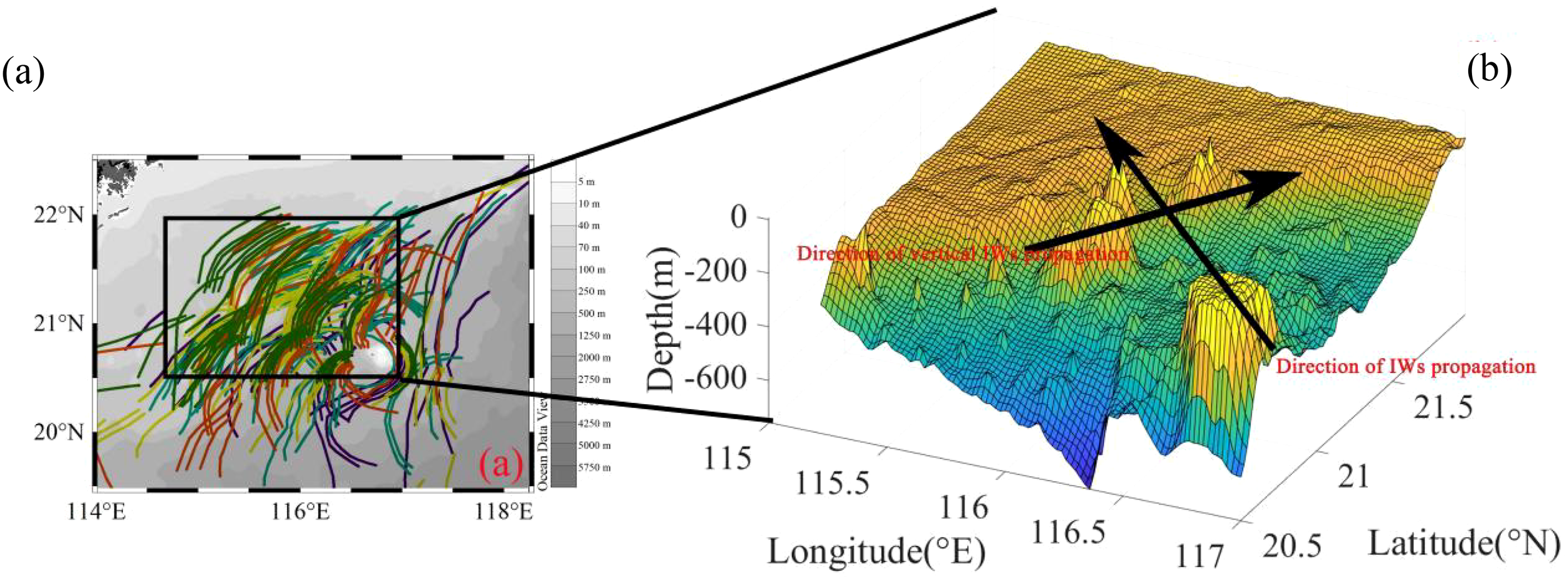
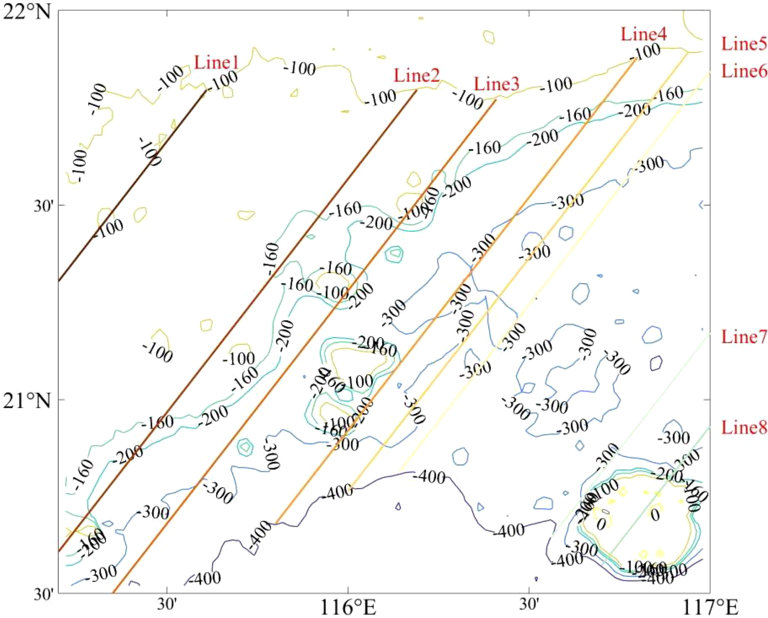
Spatial distribution of IWs from May 6 to 10, 2020, with (a) the black dashed box showing the range of effect of IWs after passing through the DA and (b) the bathymetric distribution. Black arrows indicate the direction of IW propagation and the vertical direction.
The area of propagation of IWs contains the deep-sea basin, continental slope, and continental shelf. The water depth in the SCS basin is ~4000 m; in the continental slope, it is 100–3500 m. The land slope is undulating, and the area in the northwest is larger than that in the northeast. The water depth from the continental shelf to the continental slope turn is 150–180 m. The depth of the continental shelf is generally 0–150 m, and accumulation is wide and slow (Figure 2b). The Dongsha Islands are composed of the Dongsha, Nanwei Tan, and Beiwei Tan atolls, which are the closest group of archipelagos to the mainland and are located on the continental slope in the northern SCS. The Dongsha Islands, which have a diameter of ~30 km, are a coral reef island complex composed mainly of a variety of corals, seagrasses, microorganisms, and fish species (Hung et al., 2021).
2.2 Data
IWs cause convergence and divergence of the sea surface during propagation, changing the roughness of the sea surface and producing bright and dark bands on optical and synthetic aperture radar (SAR) images. Both types of sensors have distinct advantages. However, the limited swath width of high-spatial-resolution SAR makes it difficult to capture complete large-scale IWs in some open-ocean areas, and the long revisit period does not permit continuous observations (Jackson and Alpers, 2010; Jia et al., 2018). Therefore, the MODIS (carried aboard the Aqua and Terra satellites in sun-synchronous orbits) has become the most widely used optical sensor for observing IWs. With a spatial resolution of up to 250 m and a swath bandwidth of up to 2,330 km, MODIS is easily accessible for regional surveys of IWs (Meng et al., 2022; Zhang et al., 2022) and is also suitable for this study.
SST data from Himawari-8 were selected for the study of the immediate effect of IWs on the sea surface. Himawari-8, launched into geostationary orbit by the Japan Meteorological Agency in October 2014, is a geostationary meteorological satellite orbiting 35,786 km above the equator at 140.7°E (Jiang et al., 2019). The satellite carries the Advanced Himawari Imager (AHI) with five regional imaging modes and can image in full-disk mode every 10 min, providing observations over the Asia–Pacific region. The AHI is a multiple-wavelength imager with 16 bands ranging from visible to infrared wavelengths. Its imaging resolution is 500 m or 1 km in the visible and near-infrared bands and 2 km in the infrared band, and its temporal resolution is 2.5–10 min (Taniguchi et al., 2022; Huang et al., 2023). Currently, Himwari-8 has released Level 3 version 2.1 SST and Chl-a products, including 10-min, hourly, daily, and monthly products, with spatial resolutions of 2 and 5 km, respectively. These data have been applied in other fields but have rarely been used to study the ecological effects of IWs (Xie et al., 2020; Xing et al., 2022; Huang et al., 2021; Huang et al., 2024). The reason for not selecting the Level 1 data of the Himawari-8 for IW observations is that the bright and dark patterns produced by IWs in optical images are observed only in sunlight, but there was no sunlight in the study area during the study time period.
3 Results
3.1 Characteristics of IWs
The characteristics of IWs in the northern SCS are revealed through sequential events, which include primarily period and velocity. Four complete sets of IW first peak lines were acquired each day from May 6 to 10, 2020, on the continental shelf (Figure 3). The IWs were in essentially the same position around 3:00 on May 7 and 9, and around 5:00 on May 6, 8, and 10, and the IWs were in essentially the same position. As the IWs propagated northwestward, the distance between the IWs at both time points became closer. After passing through the DA, the IW divided into two branches, north and south, with the southern branch being faster. The two branches intersected in the northwestern DA and then continued to move forward, still with the southern branch faster and the northern branch slower. The propagation velocity of IWs1 was calculated to be ~1.8 m/s based on the distance and time between 117°E and 118°E. In the western DA, the propagation velocities of the southern and northern branches of IWs2 were ~1.56 and ~1.23 m/s, respectively, those of IWs3 were ~1.35 and ~1.04 m/s, respectively, and those of IWs4 were ~0.83 and ~0.69 m/s, respectively.
Figure 3

Spatial distribution of the first peak line of IWs from May 6 to 10, 2020 and the water depth at its location. The black arrow shows the direction of propagation of IWs.
According to the conclusion based on the mooring data, there were two types of IW periods (full-day and half-day) on the continental slope in the northern SCS (Alford et al., 2015; Ramp et al., 2022). Combining the position and time information of IWs from satellite images indicates that the IW period in this study was a half-day. Based on the distance between incident IWs and the DA, the time of arrival of IWs at the DA was calculated to be about 11:00 and 23:00 every day. It took about 4 h for the IWs to pass through the DA, leaving the DA at about 15:00 each day and at 3:00 the next day. On May 7 and 9, the first peak of IWs was about to leave the DA at about 03:00, which was close to the calculated time (Figure 3). However, IWs recrossed at the northwestern DA after crossing the DA, so there were still IWs intersecting at the northwestern DA after 05:00. Based on the positions and propagation velocities of the reflected IWs at 03:00 and 05:00, the collision times of the reflected IWs with the incident IWs were calculated to be about 06:00 and 18:00 daily. This result was confirmed by the remote sensing image on May 6, 2020, where the distance between the reflected IW and the incident IW at 05:40 was ~1.6 km.
Therefore, IWs appear as multiple wave packets near the continental shelf break. The maximum length of a single IW close to the DA is up to 470 km. After an IW reaches the DA, the abrupt continental shelf partially transforms the single IW into a wave packet consisting of two to three consecutive isolated waves. Some IWs get reflected, and the reflected IWs collide with the subsequent incident IWs at 175.3°E. Most IWs are reconnected in the northwestern DA, and the length of the northern branch is slightly greater than that of the southern branch, but both are >100 km. After that, IWs continue to propagate to the northwest, the number of wave packets increases, and the reconnection continues to deepen, and the width of the waves decreased. Then the peaks and valleys of the first few isolated waves weaken seriously, and the north–south inner isolated waves almost reconnect. In the end, the inner IWs become almost imperceptible, with all of them forming continuous wave packets (Figure 2). This process can take 2–3 days.
3.2 Satellite imagery capturing SST changes caused by IWs
The distribution of SST at the same time and in the same space where an IW event occurs can reflect the immediate impact of the IW (Figure 4). Because most of the satellite-acquired images of IWs do not exactly match the time of the SST images, the SST images at times close to IW occurrence were selected. The only image that can match the time is that taken at May 9, 2020, at 03:00, where the streak of low temperature from the propagation of the IW can be prominently seen. The line low temperature indicated by the red arrow in Figure 4d) is generated by the IW indicated by the red arrow in Figure 4e), reflecting the rise of cold water in the subsurface by the IW. On May 7, although the location of the IW was recorded 15 min later than that of SST, the streaks of IWs can still be seen matching the distribution of low temperatures, especially in the northern and southern DA (Figure 4a). The IW event on May 8 was at 05:25, so the temperature distributions at 05:00 and 06:00 on that day are plotted (Figures 4b, c). It can be seen that an hour has passed and that the center of low temperatures produced by the incident IW near 117.5°E, 21.5°N is moving in the direction of wave propagation. The time of the May 10 SST image was 15 min earlier than that of the IW, and a low-temperature center was produced by the reconnection at 30° northwest of the DA (Figure 4f). SST data of May 6 are sparse, so the SST distribution at the same time as the IW is not shown.
Figure 4
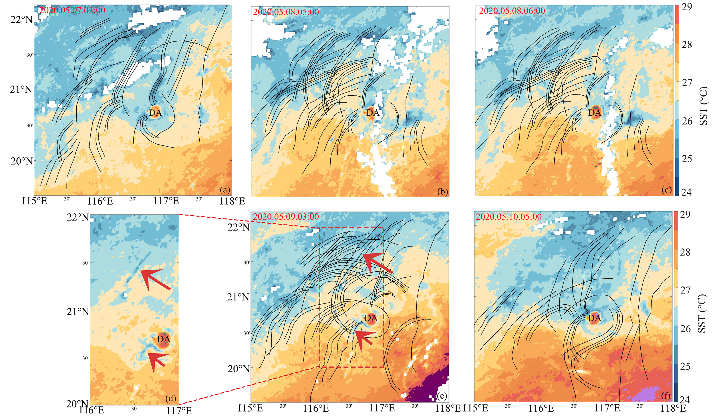
SST distribution from the Himawari satellite at 03:00 on May 7 (a), 05:00 and 06:00 on May 8 (b, c), 03:00 on May 9 (e), and 05:00 on May 10, 2020 (f). (d) is part of (e), and the black line is the distribution of the IW at an almost similar time.
According to the results in Section 3.1, the arrivals of IWs at the same time are basically at the same position. The IWs captured by remote sensing images on these days were all around 03:00 and 05:00. Because observation of the hourly variation of the IW trajectories in remote sensing images is limited, the IW trajectories at 03:00 on May 7 and May 9 were matched to May 8 and May 10, and the IW trajectories at about 05:00 on May 6, May 8, and May 10 were matched to May 7 and May 9 (Figure 5). For clarity of image representation, only the first peak line of the IW is chosen to characterize the position of the IW. On May 7, the cold center weakened from 03:00 to 05:00 at both the red and black circle locations with the passage of the IW, and the cold region moved westward with the advance of the IW (Figures 5a, b). The position of the matched IW at 03:00 on May 8 matches exactly with the center of cold water caused by the IW (black circle) (Figures 5c, d). At 05:00 on May 9, the position of the IW in the red circle was westward of the low-temperature linear region (Figures 5e, f). Because the matched IWs all occurred later than 05:00, it was normal for the IWs to occur before the cold water. The center of the cold water in the black circle position at 03:00 on May 10 also corresponds well to the IW (Figures 5g, h). The above matches between IWs and cold water demonstrate the role of IWs on SST, which can be visualized by Himawari’s high-temporal- and high-spatial-resolution data.
Figure 5
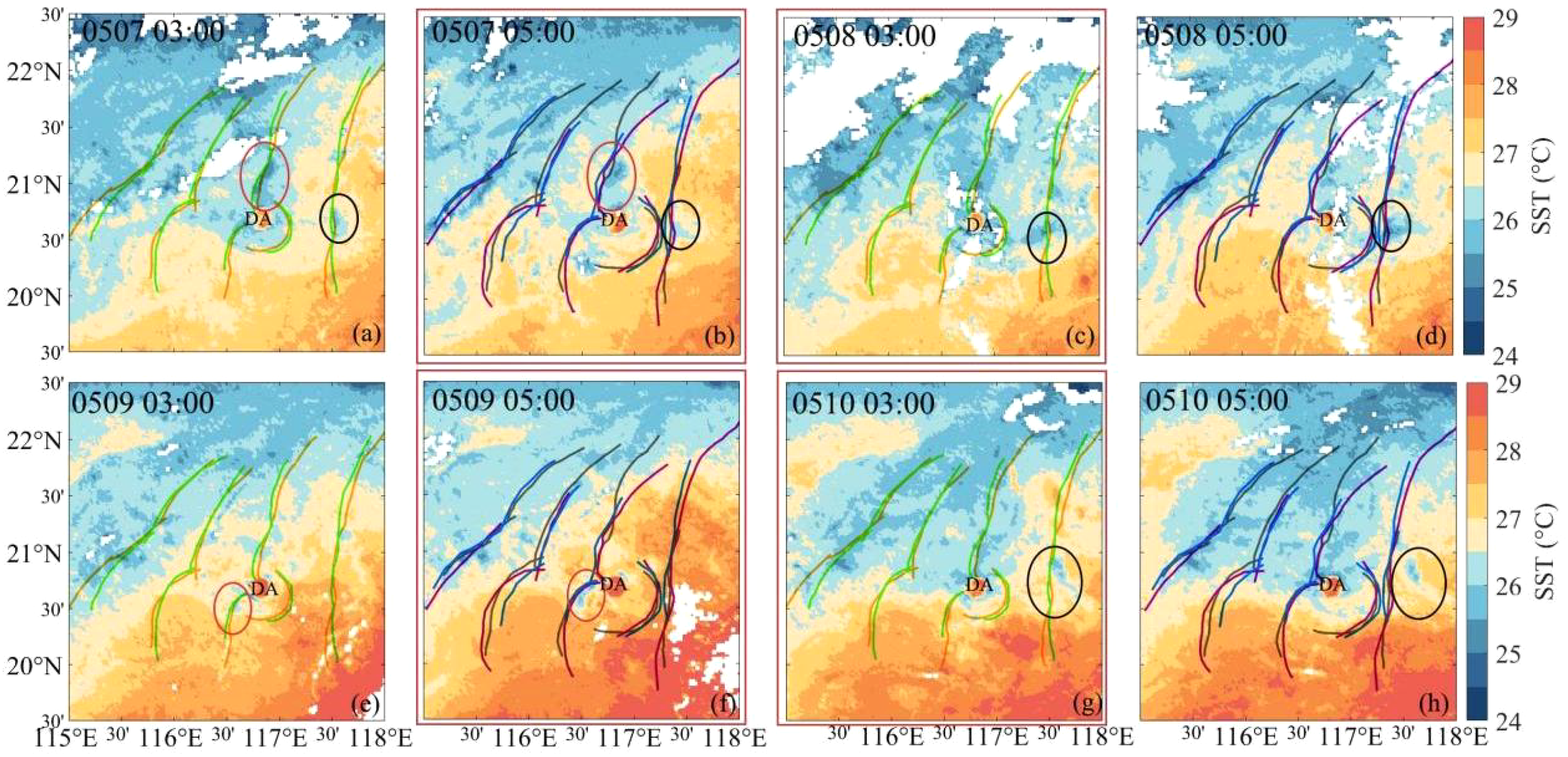
Distribution of SSTs at 03:00 (a, c, e, g) and 05:00 (b, d, f, h) on May 7–10, 2020, with red and black circles showing SSTs at the same location at different moments in time. The red boxes show the IWs matched to SST according to estimated time.
3.3 SST changes produced by different IWs in the DA
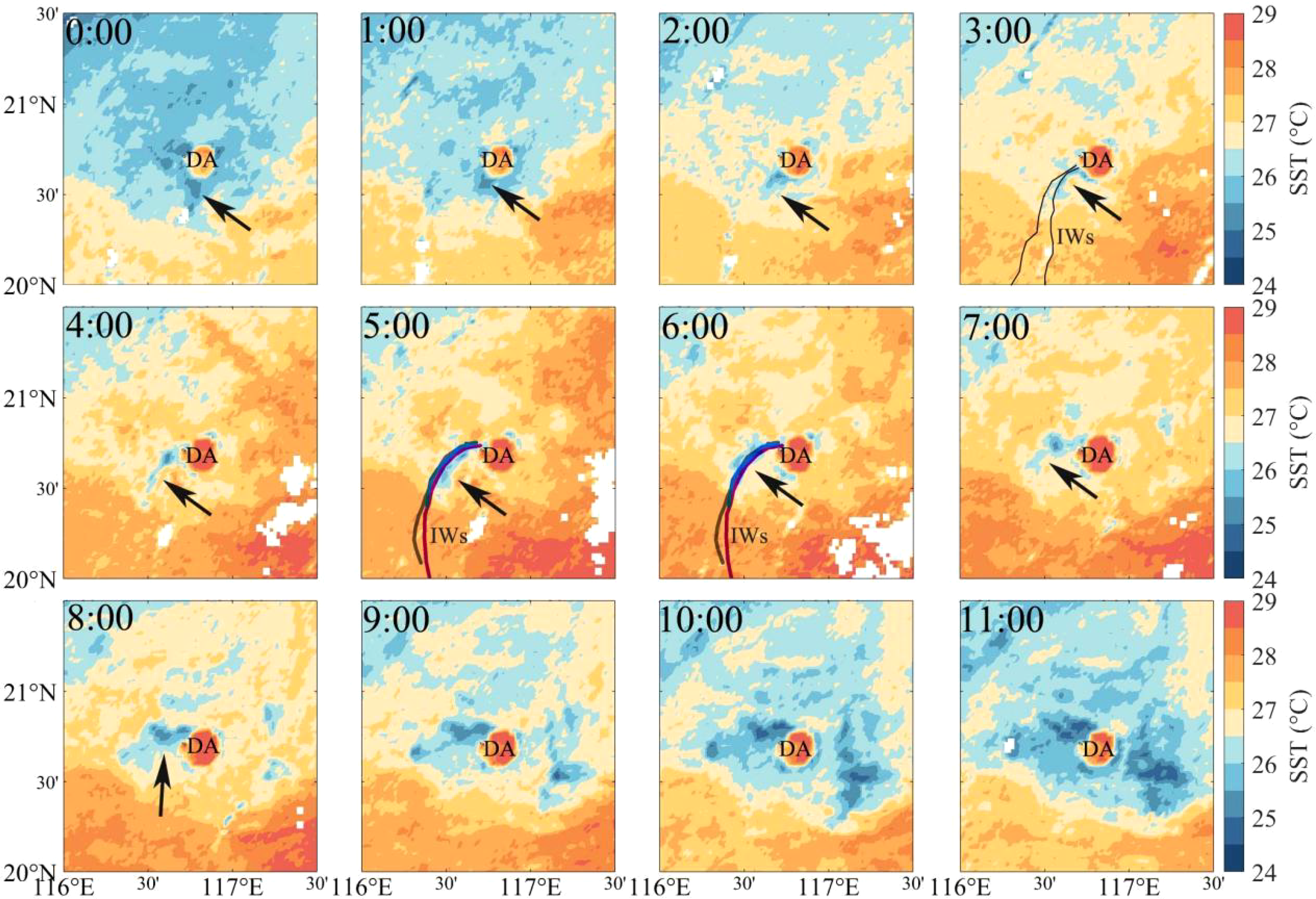
Changes in SST near the DA and on the continental shelf caused by IWs and evident on satellite images are shown in Section 3.2, but different IWs cause different SST dynamics (e.g., May 7–10). The cold water uplifted by the northern and southern branches of the IW on May 7 created a moving track of linear low temperatures in the north (black arrow), with a small area of low temperatures in the south (gray arrow) (Figure 6). The opposite was recorded on May 9, where the moving trajectory of linear low-temperature change caused by the southern branch of the IW is evident (black arrow) (Figure 7). The northern and southern branches on May 8 and 10 exhibited insignificant moving trajectories because of interference from the background temperature. The reason for not choosing the movement track after 11:00 is because the background temperature is so low that the low-temperature effect produced by the IW was not obvious.
Figure 6
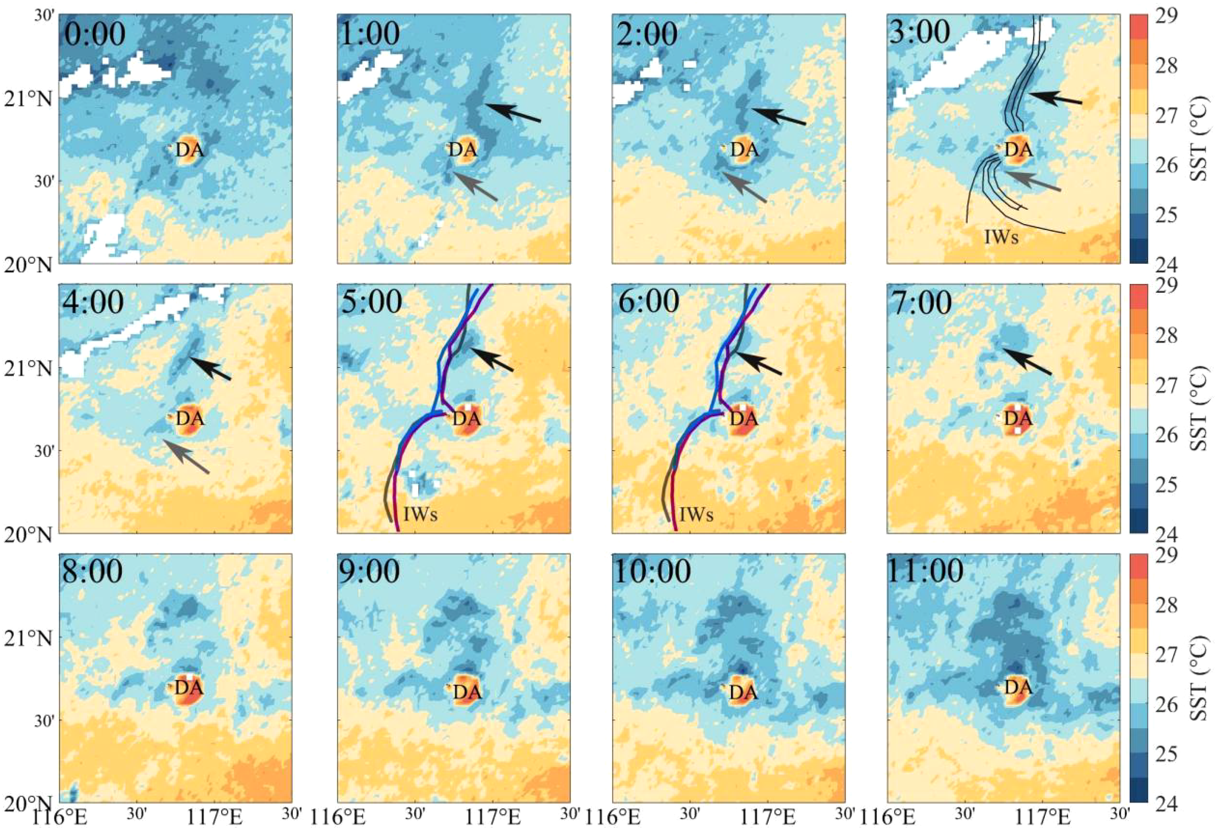
Distribution of SST dynamics in the DA on May 7, 2020, from 0:00 to 11:00. The blue, gray, and purple lines are the positions of the first peak line of the IWs at 5:40 on May 6, at 5:25 on May 8, and at 5:15 on May 10, respectively. The black line is the position of the IWs at 3:15 on May 7. The black and gray arrows indicate the changes in SST of the north and south branches of the DA, respectively.
Figure 7
Distribution of SST dynamics in the DA on May 9, 2020, from 0:00 to 11:00. The blue, gray, and purple lines are the positions of the first peak line of the IWs at 5:40 on May 6, at 5:25 on May 8, and at 5:15 on May 10, respectively. The black line is the position of the IWs at 3:00 on May 9. The black arrow indicates the changes in SST of the south branche of the DA.
The IW-induced SST dynamics for the day of May 7 are mapped hourly in Figure 6. The SST corresponding to the IW position at 03:00 shows that, at this time, the center of the IW-induced low-temperature region extended longer and over a larger range in the northern DA than in the southern DA. After the IW reached the DA at 23:00 on May 6, the temperature below 25.5°C in the eastern DA could be seen at 0:00 on May 7. As the IW separated into northern and southern branches at the DA, the low-temperature center of the northern branch moved northward from the eastern DA, while that of the southern branch moved eastward from the south. Eventually the low-temperature centers of the northern and southern branches merged at the northwestern DA. The extent of the linear low-temperature region located in the north of the DA continued to decrease with increasing background temperature to a minimum by 06:00. After 06:00, the background temperature began to decrease, and the low-temperature region to the north of the IW gradually increased, mainly appearing north and west of the DA. Notably, the center of low temperatures north of 21° in the northern DA was produced from the passage of the IW at 01:00 and then moved westward as the IW moved through. After the passing of the IW and the increase in background temperature, the linear low temperatures produced by the IW slowly disappeared, but low temperatures in the area bounded by 116.5°–117°E, 21°–21.3°N persisted for a long time. By 07:00 the low temperatures deepened as the background temperature decreased. This also occurred in the western DA at 116.5°E, 20.8°N. It is easy to see that the low-temperature region began to appear at 117.5°E at 04:00 and then moved toward the direction of the traveling IW with the passage of time, gradually connecting with the DA coupled with the decrease of the background temperature. This eventually led to a triangular area of temperature below 26°C around the DA.
SST dynamics caused by the IW on May 9 differed from those on May 7 (Figure 7). Beginning at 00:00, the IW caused the temperature to drop below 25.5°C in the southern and northeastern portions of the DA. As the IW moved, the line of low temperatures continued westward along the DA. The area of low temperatures in the southern branch was larger and more pronounced (black arrow), while the low temperatures in the northern branch existed only around the DA. Notably, at 116.5°E, 20.8°N in the northwestern DA, the low-temperature center persisted after being produced by the IW at 06:00 and was enhanced by the passing of the IW and reduction in background temperature. The cold region in the northwestern DA at 00:00 gradually disappeared as the background temperature increased until after 07:00, when the low temperature in this region reappeared and continued to decrease. This indicates that the low temperature in the northwestern DA at 0:00 is not a transient effect of the IW but rather is caused by the background temperature. The low temperature between 117°E and 117.5°E starts at 06:00, when the incident and reflected IWs collide, and the low-temperature region keeps moving westward with time as the incident IW continues to move toward the DA. The background temperature deepened the low temperature to some extent.
The May 7 and May 9 IW-induced low temperatures were notable in the northern and southern branches of the DA, respectively. The May 7 low temperature in the northern branch led to a certain area of low temperatures north of the DA, but the May 9 low temperature in the southern branch did not persist in the south. After the intersection of the northern and southern branches in the northwestern DA, the low temperature of the IW on May 7 was still distributed along the northern and southern sides, with a small area of low temperature at the intersection, while the low temperature at the intersection of the IW on May 9 was persistent and extended in the direction of the movement of the IW. The location of the low temperature generated by the collision between the incident IW and the reflected IW is related to the moving position of the reflected IW. The moving direction of the reflected IW on May 7 is 5° southeast, while the moving direction of the reflected IW on May 9 is 30° southeast, so the distribution of the low-temperature area on the right side of the DA is different from the angle of the DA.
In summary, the different IWs all produce low-temperature regions around the DA but at different locations. These include the linear low-temperature region caused by the movement of the northern and southern branches of the IW, as well as the low-temperature patch caused by the collision of the IW at the intersection and caused by the collision of the incident IW and the reflected IW. Linear low temperatures at the sea surface caused by the movement of the IW disappear within an hour, but in some locations the low temperatures persist longer.
3.4 Process analysis of SST changes resulting from IWs in the northern SCS
Because SST data on May 6 are sparse, the hourly SST data of May 7–10 were averaged to illustrate the whole process of SST change caused by the propagation of IWs over the northern continental shelf of the SCS (Figure 8). The results of Section 3.1 showed that the daily continental slope contains IWs that reached the DA on that day, the IW packets that propagated for two days, as well as incoming IWs that did not arrive and IW packets that were reflected by the DA. The background temperature was calculated daily in the area 115°–120°E, 19°–22°N in the northern SCS because the variation of the background temperature during the day has an impact on the study of the effect of IWs on SST (not shown). The background highest SST of the day is at 06:00, after which it decreases until 22:00 when the background lowest SST of the day occurs, and then SST starts to rise again on a daily basis.
Figure 8
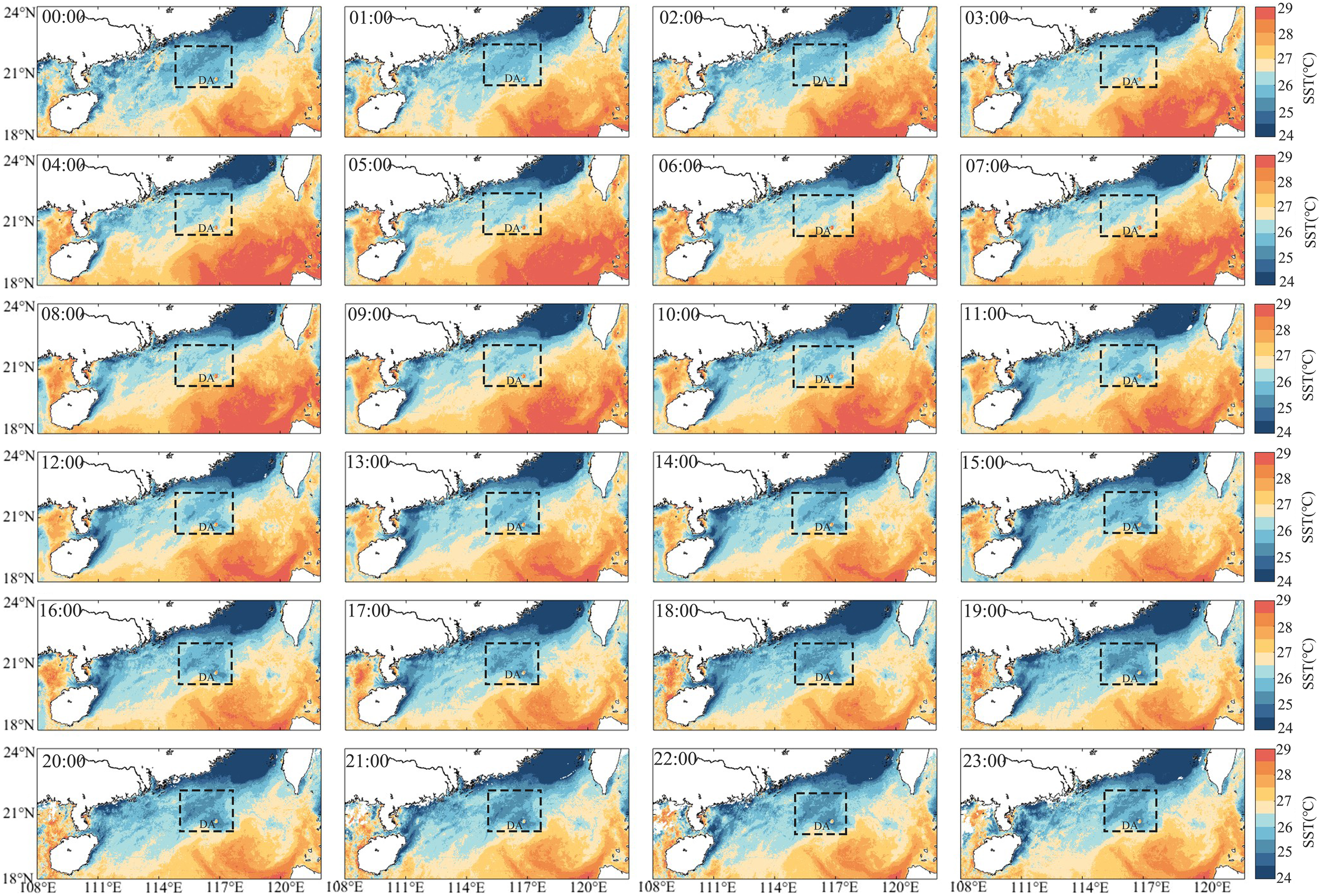
Hourly variation in SST under the influence of IWs during a day. The black box shows the study area.
Overall, the regions with significant SST dynamics during the propagation of IWs were the DA and the western SCS, which were the areas we focused on (Figure 8). During the period of increasing background temperature from 0:00 to 06:00, the region of low temperature in the northwest SCS caused by IWs was decreasing, and the region below 26°C was located around the DA and on the connecting line between 115°E, 20°N and 116°E, 22°N. Beginning at 04:00, a low-temperature region also appeared in the eastern DA as a result of the incident IWs. The area of low temperatures east of the DA moved all the way to the DA over time, stopped moving, and eventually connected with the DA by 09:00. Between 07:00 and 22:00, the background temperature continued to decrease, and the low-temperature area around the DA kept increasing, mainly to the north and east. The low-temperature region in the northern shelf area of the SCS was distributed in strips parallel to the coast, with temperatures below 25.5°C occurring at two locations, 115.5E, 21°N and 117E, 22°E. And the range in size of the low-temperature region varied with the change in the background temperature. Finally, the low-temperature region in the northwestern SCS shelf area is connected with the low-temperature region around the DA became triangular. Temperatures below 25°C around the DA appeared in the southeast at the location of the interaction with the DA and in the northwest at the intersection of the IWs. After 22:00, the background temperature increased, and the temperature region below 25°C in the northwestern SCS shelf area and around the DA almost disappeared, leaving only the IW intersection in the northwestern DA.
In addition, one phenomena of interest can illustrate the different performance of IW-induced low temperatures and background-temperature-induced temperature reduction. From 04:00 to 06:00, the low temperatures generated by incident waves that appeared in the eastern DA kept moving in the direction of IW propagation. Meanwhile, the background temperature continued to increase during this period, but the low-temperature range of 25.5°C–26°C remained almost constant. From 07:00 onward, the region of low temperature became larger, and the region of low temperature below 26°C became connected to the DA at 09:00. It is obvious that the low temperature was caused by IWs before 06:00, and the change in SST was the result of the low-temperature dissipation process generated by the passage of IWs balanced with the process of increasing background temperature, with the low-temperature region rapidly becoming larger after 07:00 because of the decrease in background temperature.
It is found that, in the western DA, SST is consistently very high, and there are areas of low temperature slowly appearing in the deep-sea region after 10:00, which may be caused by the shedding eddies (Wang et al., 2017).
4 Discussion
4.1 Effect of water depth on IW propagation
Years of optical and SAR IW remote sensing data reveal that IWs propagate at a speed of ~2 m/s when they propagate to the west near the DA, gradually slow to a velocity of ~1 m/s when propagating toward the shelf slope, and slow to <1 m/s when arriving at the shallow waters of the continental shelf (Sun et al., 2018). Mooring data near the DA showed that the propagation speed of IWs was 1.05 m/s at a water depth of 200–300 m, 0.7–0.8 m/s at depths below 200 m, and as low as 0.4 m/s at a water depth of 100 m (Fu et al., 2012). Therefore, the IW velocities calculated from satellite data and measured are consistent with the range of IW propagation velocities at different water depths in this study.
The depth of water decreases from south to north in the IW propagation path. Before reaching the DA, the position of IWs in the north of 21.5°E lag behind that of the southern part at the same time. Starting from the arrival of IWs at the DA, IWs get divided into two branches, and the velocity of the northern branch starts to be significantly lower than that of the southern branch, which results in the intersection of the two branches being located at ~36° northwest instead of west. During propagation, with the further influence of water depth, the velocity of the southern branch of the IWs is always higher than that of the northern branch. Consequently, the intersection is constantly shifted, and the northwestward angle increases. The water depth of the IWs3 is shallower than 300 m, so the IWs3 to IWs2 intersection is only slightly shifted by ~20° northwest (Figure 3). However, the water depth of the IWs4 compared to that of the IWs3 is much shallower, and the offset of the intersection is greater, being ~40° northwest. During the same time period, the propagation distance of the southern branch of the IWs is greater than that of the northern branch, and finally the direction of IW propagation shifts from westward to perpendicular to the direction of the continental shelf.
The change in the propagation speed of the internal wave by the depth of the water leads to a change in the direction of propagation, which also leads to a change in the angle of collision between the reflected and incident waves in the eastern DA. The point of collision of incident waves reflected at DA is generally not eastward of the DA but southeast. In addition, the IW velocity is low in the north but high in the south. Therefore, the center of the semicircle of the reflected IWs is often not in the eastern direction of the DA, but in the southeastern direction. The location of collision with incident IWs also tends to occur southeast of DA rather than east. The statistics of 100 sets of incident IWs and 70 sets of reflected IWs near the DA indicate that incident IWs with angles of 270°–300° account for >80% of the total, while reflected IWs with angles of 90°–120° account for nearly 60% of the total. And the proportion of both incident and reflected IWs with this angle is the greatest (Zhang et al., 2018). The incident and reflected IWs in this study belong to the most common types. Of course, there are other cases in which the northern and southern IW branches can be reconnected at the southwestern DA and the incident and reflected IWs collide at the northeastern DA, which may be related to ocean stratification, background currents, and the initial wave amplitude (Jia et al., 2018).
4.2 Analysis of the mechanism of SST changes caused by IWs
What is obvious in SST changes caused by IWs is that not all regions through which they pass are elevated by cold water. During the passage of IWs, low temperatures occur in specific areas (Figure 4). In the 24-h SST variation, the overall SST in the area of IW propagation (<26.5°C) is lower than that in the surrounding sea area, and the colder SST areas are mainly concentrated near the DA and on the continental shelf surface (Figure 9), which have different characteristics of SST variation. The low-temperature region near the DA is distributed in three locations: its northern, northwestern, and southeastern parts. In the northern DA there is a mixing of low temperatures caused by the interaction of IWs and topography due to the shallow water depth. Northwestern and southeastern DA are the areas where IWs meet and where collision of incident and reflected IWs occurs. This enhances the vertical transport of internal waves and leading to more cold water being brought to the surface, creating significant low temperatures (Muacho et al., 2014). The low temperatures on the continental shelf surface are located at water depths of 100-200 m, which are caused by turbulent mixing of the internal waves due to strong interaction with the shallow topography, especially near 200 m where the sudden change in water depth leads to the breakup of the IWs causing stronger low temperatures (Ramp et al., 2022).
Figure 9
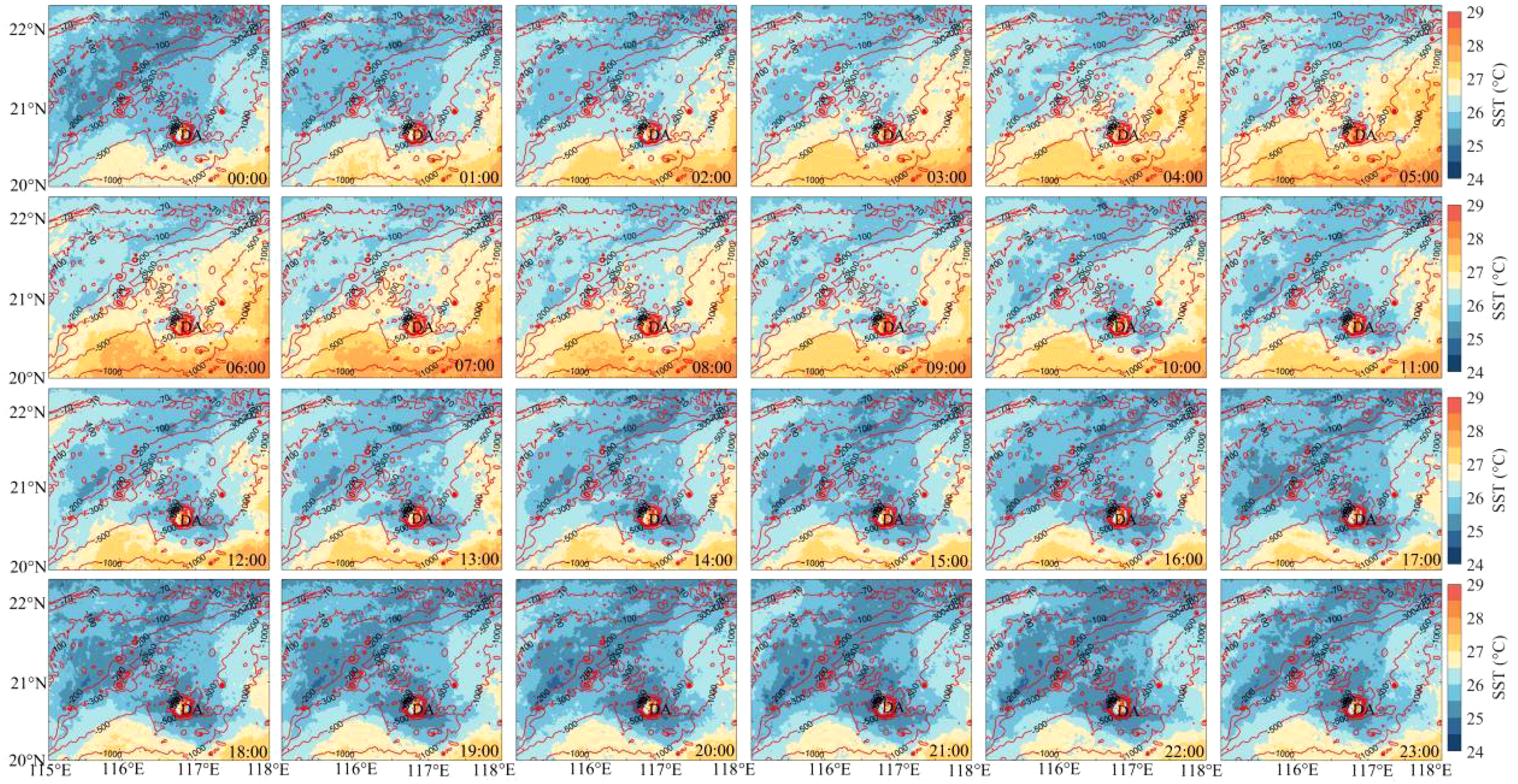
Hourly distribution of SST in the northwestern SCS, with bathymetric isobaths in red.
However, in the middle of these two low-temperature regions, the DA and the continental shelf surface, the temperature is not continuous in the propagation path of the IWs. During the propagation to the northwest, the IWs continuously experiences energy dissipation, the propagation speed decreases, the wavelength becomes longer, and the amplitude becomes shorter. After passing through the DA, at a water depth of 350 m, the amplitude of the IW is shallower than 250 m and the wavelength exceeds 6 km (Gong et al., 2021). Therefore, the vertical transportation of cold water by IWs is more than 6 km apart between the two low-temperature regions, and the whole process lasts no more than 2 hours (Wang et al., 2017), so the low-temperature effect is not significant.
Meanwhile, we found that the low temperatures caused by turbulent mixing due to the shoaling effect had a long duration, while those caused by vertical movement had a short duration. High-frequency IWs in the SCS shelf area are generated by the shallow fission of IWs (Bai et al., 2019), and the turbulent mixing induced by fission is slightly weaker, lasting long enough to contribute to mixing in the gentle shelf area. Fracturing and dissipation are the endpoints of the evolutionary development of IWs and the energy dissipation processes of turbulence generation and conversion of mechanical energy into internal energy, which is often accompanied by enhanced mixing of seawater (Sutherland et al., 2015). At the same time, IW breaking by shear instability and convective instability dominates IW energy dissipation and is the main source of energy for mixing across density surfaces within the ocean (Garrett and Kunze, 2007). Although the dynamics of turbulent mixing is not as strong as that of vertical convection (Liu and Lozovatsky, 2012), the IW propagates as an isolated wave at a water depth of 200 m, but after the depth near 200 m the IW breaks up into a wave packet (Figure 1), which continuously breaks up to form more wave packets, so that the low temperature caused by an isolated wave is presented as a line, while turbulent mixing caused by wave packets is prone to form a large area of low temperature (Figure 9).
The continental shelf low-temperature surface occurs at water depths of 100–200 m and consists of two low-temperature centers (Figure 9). The center of one low-temperature region is located at 115.5°E, 21°N, with a depth of <200 m, and the topography may play an important role. The semidiurnal IWs impinge obliquely on the southwest–northeast slope and break up near the bottom because of critical supercritical reflections, significantly dissipating energy, and the location of their energy dissipation coincides with most of the low-temperature region (Xie et al., 2018). The other region of low temperature is located north of 21.5°, shallower than 200 m, and this region is densely populated with 200-, 100-, and 70-m isobaths. The northern branch of IWs breaks up here in the region of drastic changes in water depth, thus causing another low-temperature region in the northwestern DA.
The shoaling effect of IWs has been shown to raise cold and nutrient-rich groundwater in the continental shelf and nearshore environments to nutrient-depleted surfaces (Woodson, 2018; Reid et al., 2019). Observations from the mooring array revealed that IWs did not interact with the topography at sites with water depths of ~500 m. At depths of 200–300 m, the waveforms evolved in a distinctly asymmetric form. At depths shallower than 200 m, the IWs interacted with the topography and then cold water at the bottom appearing between the waves (Hung et al., 2021). Notable is that the results of this study are the same as the conclusions on the role of IWs and topography drawn from Huang et al (2021) study on the northeastern DA, where the mooring arrays are located but, in addition, this study reveals all the regions of IW action in the northwestern SCS. At the same location as the mooring array, the cryogenic region is indeed confined to an area shallower than 300 m in 24 h (Figure 9). However, in the southeastern DA, the low-temperature area is larger and is not only distributed around the DA. This may be related to the underwater reefs in the southeastern DA, or it may be caused by the collision of reflected and incident IWs. The conclusion that shoaling activity of different intensities may occur at the same location has been frequently mentioned in previous empirical studies (Fu et al., 2012; Chen et al., 2016; Villamaña et al., 2017), and this is confirmed by the 24-h temperature variations. The region of IW-induced cold water is concentrated near the DA and between ~100 and 300 m on the continental shelf, and the region of very low temperature occurs repeatedly at the same location. For example, for 116.5°–117°E, 21°–21.3°N and 116.5°E, 20.8°N, the former and the latter can be seen to occur at water depths below the 200-m isobath in the northern and western DA (black circle), respectively (Figure 3). Similar results were obtained after CELT model simulations using DA cross-slope oriented mooring data, where near-bottom intensification and rupture of diurnal internal tides may occur on slopes in water depths of 160 to 110 m, and they are confined to a depth range of ~100 m near the seafloor (Xie et al., 2018).
4.3 Immediate effects of IWs on SST in the northwestern SCS
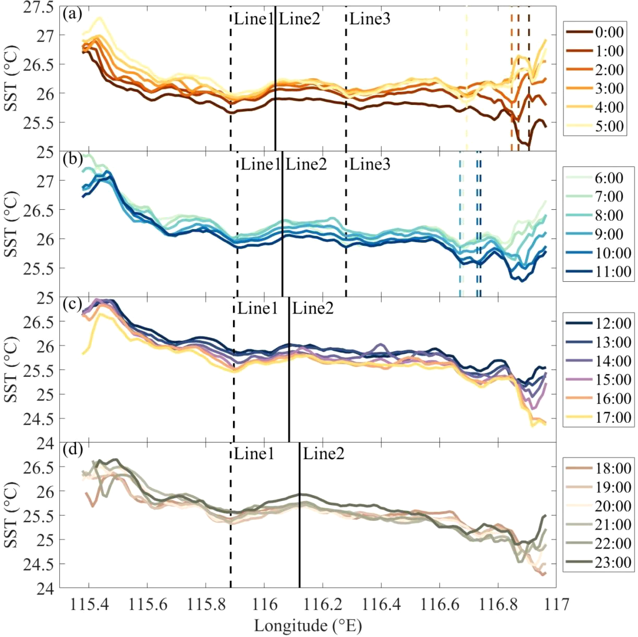
The extent of the region of cold water induced by IWs in the northwestern SCS is well defined. To investigate how SST changes with water depth during propagation, we selected the region 115.2°–117°E and 20.5°–21°N, which are shallower than 400 m, on May 9 and 10, 2020. The SST change perpendicular to the direction of IW advance over 24 h can illustrate the immediate low-temperature phenomenon induced by IWs. Overall, SST increases until 06:00 and then decreases until 22:00, and sea surface then starts to warm again at 23:00, which reflects the change in the background SST. However, the difference from the background SST is that the hourly variation of the SST produced by the passing of IWs through the DA position is more significant from 0:00 to 11:00. The location of the minimum SST induced by IWs in the DA from 0:00 to 07:00 moved westward with their westward propagation, advancing from 116.87°E (where SST = 25.5°C at 0:00) to 116.66°E (where SST = 26.7°C at 07:00) (Figures 10a, b), where the water depth was 300 m (Figure 11). After that, as IWs advanced to the west, the position of the minimum SST in the water depth did not move forward, but rather it returned to appear at a shallower isobath; that is, the location of the minimum SST began to slowly return to the northwestern intersection of the DA (Figure 11). At 116.6°E to 116.9°E, after passage of IWs, SST at the DA increased to form a peak, while low SST persisted at the northwestern intersection of the DA (Figures 10a, b). The values of SST around the DA did not exhibit a significant trend because of the effect of the decrease in the background SST after 11:00 (Figure 10c), and the low SST (24.9°C) caused by IWs reappeared at 116.91°E after the SST increased at 23:00 (Figure 10d). Moreover, the centers of cold water generated during propagation are not uniformly distributed. In addition to the effect of variations in IW speed, there may be a correlation with differences in the intensity of the low temperatures caused by the depth of the water during IW passage (Jia et al., 2018).
Figure 10
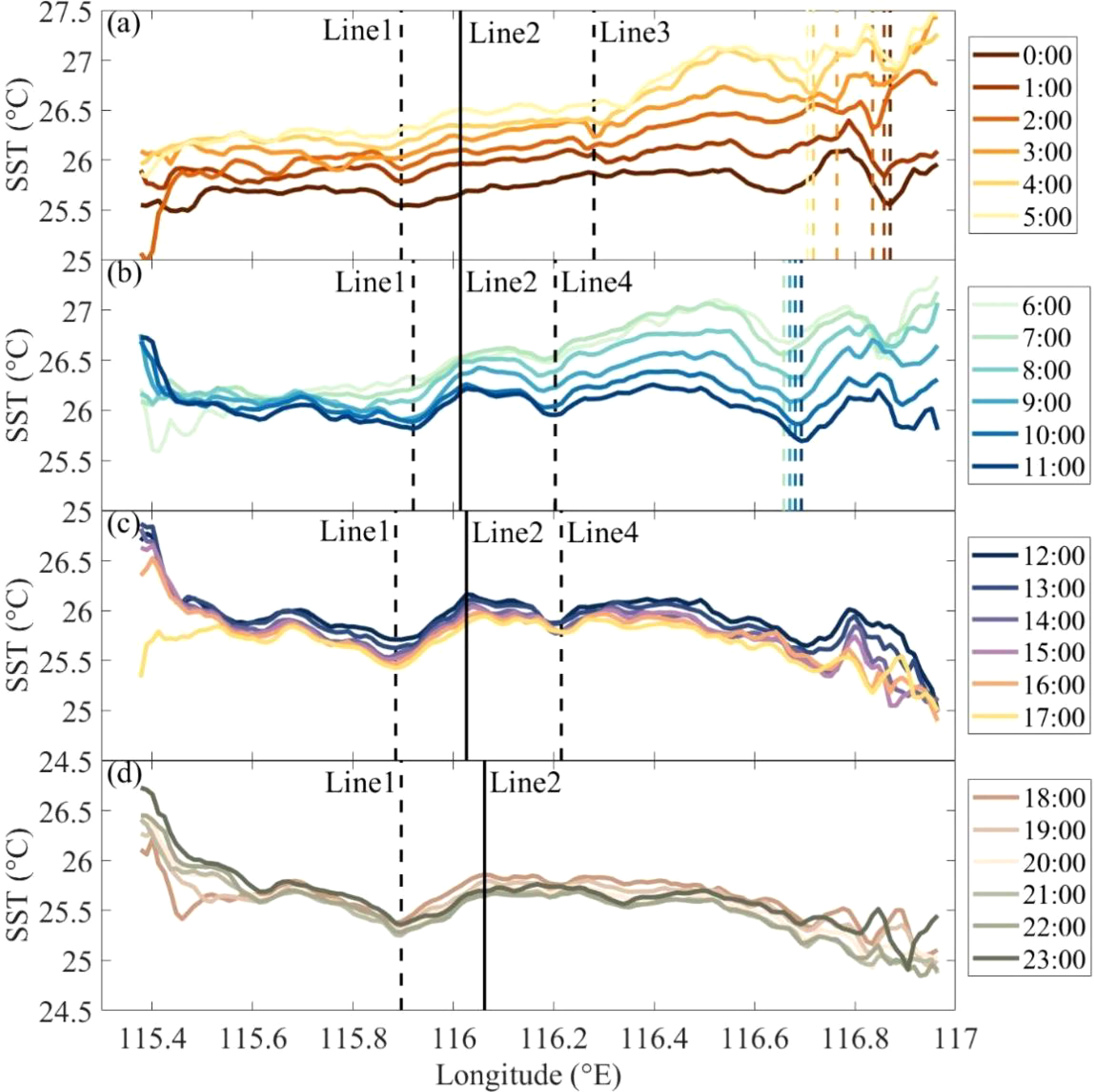
Hourly SST changes for the 24-h (a–d) period on May 9, 2020, with the region showing the propagation direction of IWs in Figure 2b). Line1 to Line4 show the feature locations during the advance of IWs. The locations of low SSTs caused by these IWs from 0:00 to 11:00 correspond to their respective time color scales (a, b). The locations of the lowest SSTs are the same for 06:00, 08:00, and 09:00 (b), with the colors being overlaid by those of the 09:00 time scales.
Figure 11
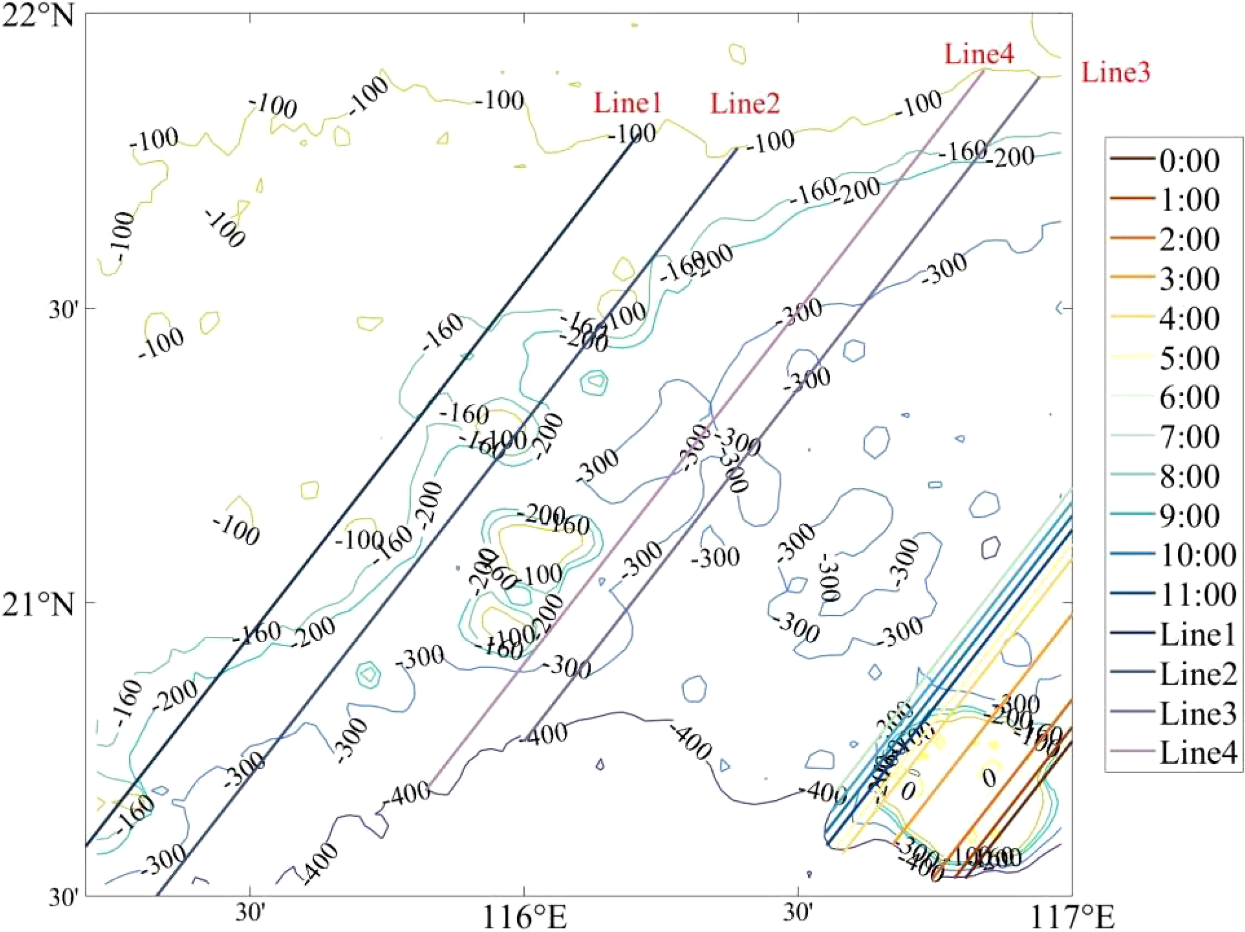
Geographic locations corresponding to features in the direction of propagation of IWs on May 9, 2020, in Figure 10, including geographic locations corresponding to low SSTs caused by these IWs from 0:00 to 11:00.
In addition to the changes around the DA, SST valleys were observed at 115.9°E (Line1 in Figure 10a) and 116.28°E (Line3 in Figure 10a) from 0:00 to 05:00. The valley near 115.92°E has been present and deepened with time, the valley at 116.28°E has been weakening with time, and the SST valley at 116.2°E has also appeared from 06:00 to 11:00, increasing and then weakening. There is no corresponding satellite image to show the trajectory of IWs, and discussion of the correspondence between the SST change and the position of IWs will be postponed. Line2 is the location (116.01°E) where SST begins to drop before the appearance of the SST valley at 115.92°E (Line1 in Figure 10a), and this location moves all the way to the direction of the arrival of IWs as the background SST decreases. SST valleys in Line3 (Figure 10a) have a shorter distance to drop, so the position of the beginning of the SST drop is not labeled. It can be seen that the two SST valleys in Line3 (Figure 11) occurred at the edge of the reef at water depths of 300 and 200 m, respectively, whereas the low SST at 115.92°E starts at a depth of 200 m, and the lowest value occurs in water depths shallower than 160 m. The high SST to the west of 115.4°E may have been influenced by coastal water.
Comparing with the hourly SST changes on May 9, the lowest SST in the eastern DA on May 10 also remained at a water depth of 300 m at 06:00 (Figures 12a, b), and the final lowest SST position also remained at the intersection of the IWs in the western DA (Figure 13). On the continental slope of the SCS, the location of the minimum SST as shallow as 200 m and shallower than 200 m (115.9°E) was the same as on May 9 (Figure 13). However, the two locations of low SSTs between water depths of 300 and 200 m are not significant, and only a weak decrease in SST (0.1°C) can be observed at Line3 (116.28°E) from 0:00 to 11:00, with an even weaker decrease produced at 116.21°E (not shown) (Figures 12c, d). The distribution of minimum SST at depths of <200 m is relatively stable, and the position is slightly nudged to the west in response to the disturbance of background SST.
Figure 12
Hourly SST changes for the 24-h (a–d) period on May 10, 2020, with the region showing the propagation direction of IWs in Figure 2b). Line1 to Line4 show the feature locations during the advance of IWs. The locations of low SSTs caused by these IWs from 0:00 to 11:00 correspond to their respective time color scales (a, b). The locations of the lowest SSTs are the same for 03:00, 04:00, and 05:00, with the colors being overlaid by those of the 05:00 time scales. The locations of the lowest SSTs are the same for 07:00, 08:00, and 09:00 (b), with the colors being overlaid by those of the 09:00 time scales.
Figure 13
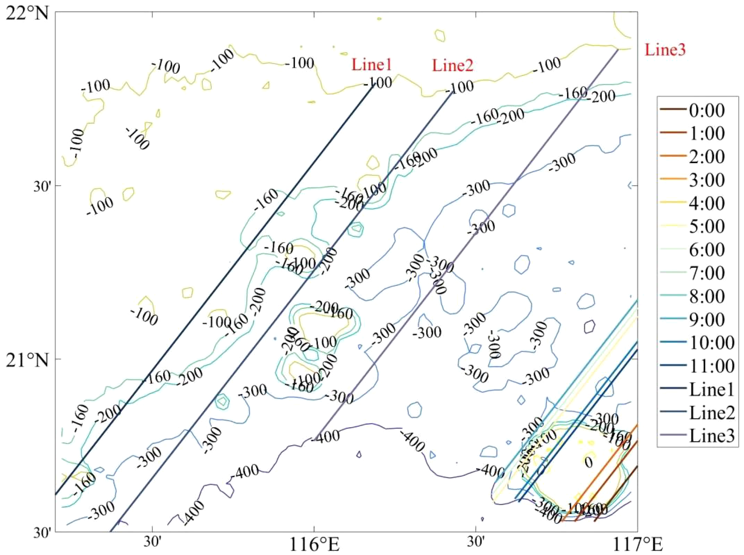
Geographic locations corresponding to features in the direction of propagation of IWs on May 10, 2020, in Figure 12, including geographic locations corresponding to low SSTs caused by these IWs from 0:00 to 11:00.
Therefore, it can be found that due to the effect of topography, the low temperature induced by IWs in the near of DA varies with the movement of IWs. But as the IWs leave DA and continue to propagate to the northwestern of the continental shelf, the effect of the low temperature induced by the vertical transportation of the IWs is not significant, and the extreme low value of the IWs still exists in the near of DA. When the IW propagates to the shallow water depth of 300 m on the continental shelf, the IW transformation caused by the shoaling effect and the turbulence caused by the topography and internal wave breakup play a role again, and cause a significant low temperature region at specific locations (e.g., reefs, seamounts).
4.4 Long-term effects of IWs on SST in the northwestern SCS
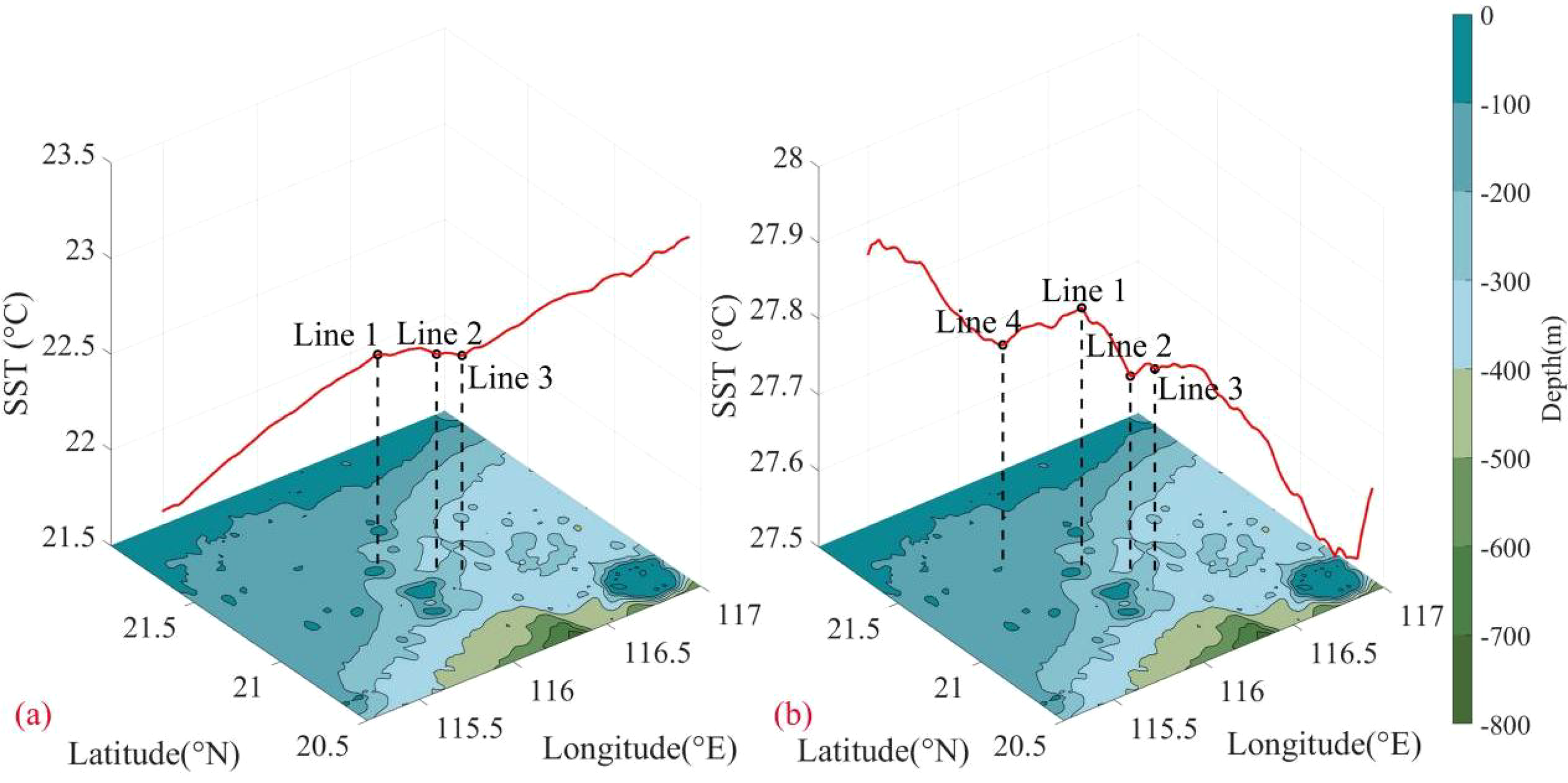
MODIS satellite image data showed that IWs occurred every day in May 2020. Comparison of SSTs of the daily averages on May 9 and 10, 2020, the monthly average of May, and the annual averages of May 2016–2023 revealed the same pattern on the continental slope of the SCS. The low-temperature regions were all between 115.7°E (Line1) and 116.02°E (Line3) and between 116.15°E (Line4) and 116.6°E (Line7), and the low-temperature valleys were at 115.89°E, 116.28°E, and 116.34°E (Figure 14). Water depths of 300 m (Line7) and 200 m (Line3) were thus used as the dividing line (Figure 15). Between 116.15°E (Line4) and 116.6°E (Line7), two valleys of low temperatures occurred at the 300-m water depth isobath. It is noteworthy that for the SST valleys with water depths shallower than 200 and 300 m, the former is significantly lower than the latter in the daily, but the difference between these two is not significant in May 2020. In contrast, the former is higher than the latter in the annual average distribution in May (Figure 14). SSTs are less disturbed in the two-day daily variability event, but the long time series of sea surface variability is influenced by other marine environmental factors, such as wind. At depths shallower than 200 m, SST decreases rapidly as the water depth decreases to reach a valley (115.89°E) and then SST increases rapidly in the daily average, but the monthly averages and yearly averages for the month of May indicate that SST remains essentially unchanged until being affected by the influence of coastal water. So the monthly and annual average SSTs in May mask some information. Changes in SST due to IWs can be captured at the hourly level, but changes on long time scales are difficult to quantify. At the intersection of IWs in the western DA, the daily averaged valley at a water depth of 100 m (116.71°E) was anomalously significant (Line 9 in Figure 15), the center of cold water changed little in the monthly and yearly averaged distributions in May (Line 8 in Figure 15).
Figure 14
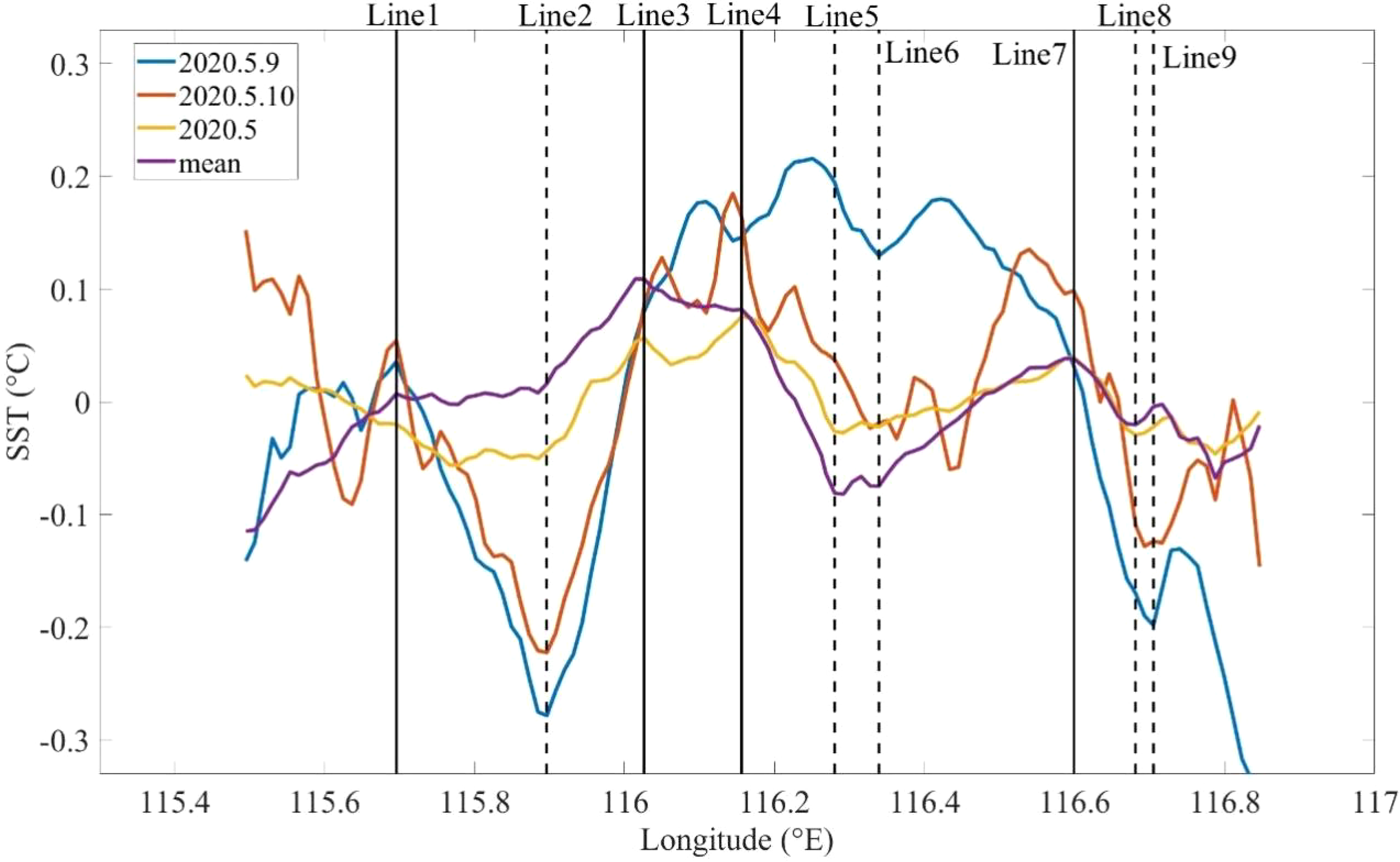
SST changes in the propagation direction of IWs in Figure 2b) for May 9, 2020 (2020.5.9), May 10, 2020 (2020.5.10), May 2020 monthly mean (2020.5), and May 2016–2023 yearly mean (mean). Line1 to Line9 are the characteristic positions during the advance of IWs.
Figure 15

Geographic locations of features in the direction of IW propagation corresponding to May 9, 2020 (2020.5.9), May 10, 2020 (2020.5.10), May 2020 monthly mean (2020.5), and May 2016–2023 yearly mean in Figure 14 in the direction of IW propagation.
Detrending the January–December climatological data from 2016–2023 reveals the significant effect of IWs on SST in the northwestern SCS. There are obvious features in the propagation path of IWs: Six SST valleys are located at 115.89°E, 116.20°E, 116.28°E, 116.34°E, 116.67°E, and 116.79°E, and one SST peak is located at 116.03°E, and these features are present in all 12 months (Figure 16). However, the SST change node located at 115.54°E occurs only in May–August, which are the months when IWs occur more frequently. Overall, from the continental slope to the DA, SST exhibits a clear trend of increasing and then decreasing in January–March and November–December. The increasing trend of SST from the coast to the far sea diminishes at 115.89°E at a water depth of ~160 m (Line 2 in Figure 17), and the increasing trend of SST is completely arrested at 116.03°E at a water depth of ~200 m (Line 3 in Figure 17); this is followed by three SST valleys (Line4 to Line6 in Figure 17) very weakly at a water depth of 300 m. SST increases again until it reaches the DA, where two SST valleys (Line7 to Line8 in Figure 17) occur at the IW intersection and at a water depth of 300 m in the northeast DA (Figure 16).
Figure 16
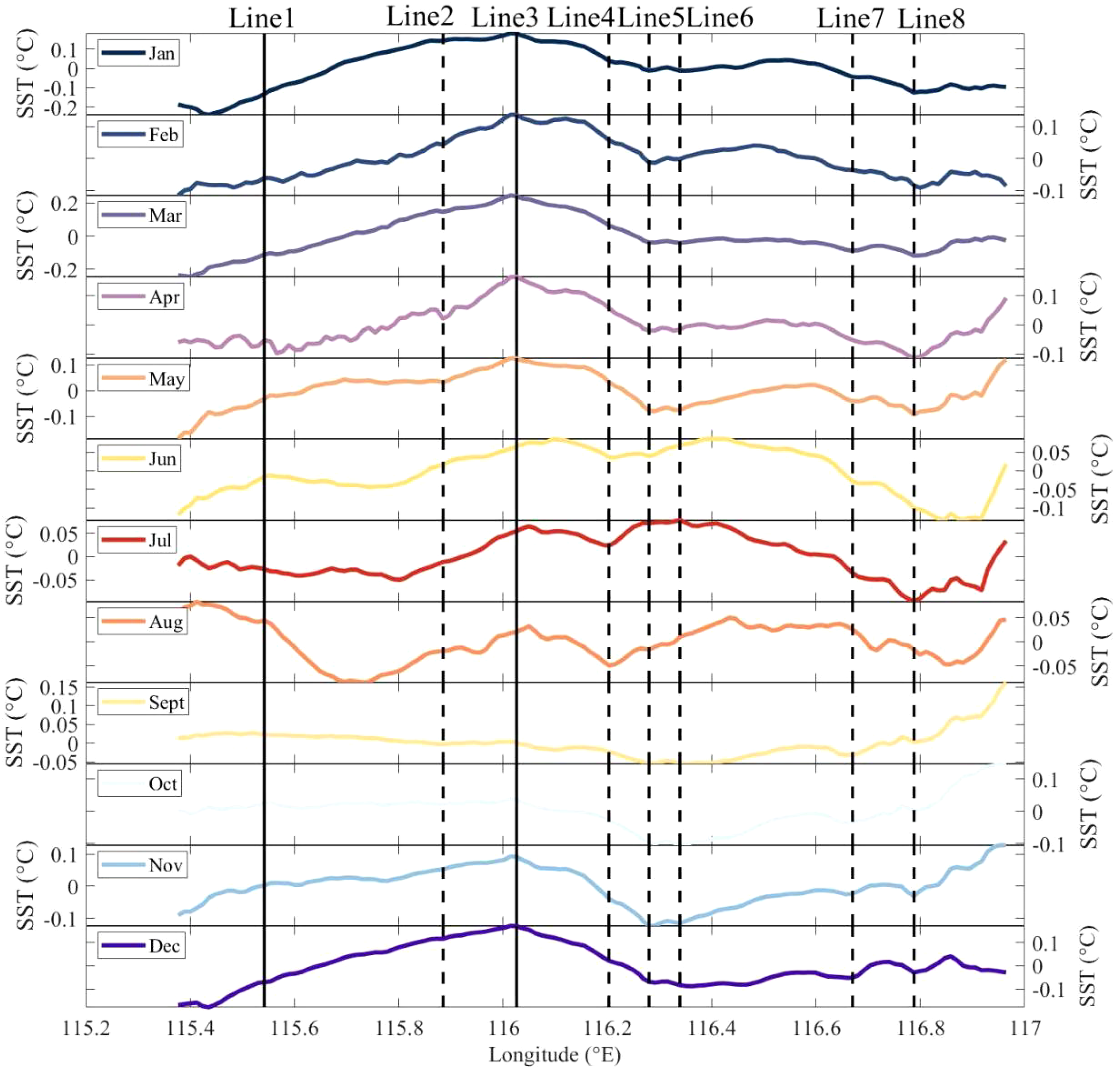
SST detrending changes in the propagation direction of IWs in Figure 2b) in January–December 2016–2023. Line1 to Line8 are the feature locations during the advance of IWs.
Figure 17
Geographic location of the feature in the direction of IW propagation corresponding to the January–December monthly mean detrended SSTs from 2016 to 2023 in Figure 16.
However, from April onward, the SST trend that had been rising from the continental slope weakened (Line 2 in Figure 17). In May, there was no longer an increasing trend between 115.7°E and 115.89°E, and SST began to decline in June until reaching its lowest point in August, when a distinct valley appeared and its position moved all the way to the continental slope, with the change in SST ending at the westernmost point at 115.54°E. The downward trend in SST tapered off in September, did not increase or decrease in October, and the upward trend resumed from the continental slope to the far ocean in November–December. During this process, the SST peak originally located at 116.02°E was slightly shifted to the east; that is, the displacement that began to produce the low-temperature change was shifted toward the DA. Among the three SST valleys at a water depth of 300 m, the one at 116.20°E (Line4), which is much shallower, kept deepening, becoming more significant in June–August, while the other two valleys (at 116.28°E and 116.34°E) (Line5 to Line6) exhibited a slight variation with the intensity of the background SST and were always present. The SST valley (at 116.79°E, Line7) located at the water depth of 300 m at the intersection near the DA also shifted to the east at a water depth of 100 m during April–September and was most significant in August. Meanwhile, the low SST interval (at 116.67°E, Line8) located in the middle of the DA widened (Figure 16).
The results of the 12-month climatological SST are consistent with the frequency of occurrence of IWs. Meng et al.’s (2022) remote sensing survey of IWs in the SCS using >70,000 MODIS and SAR images from June 2010 to May 2020 uncovered that IWs rarely occur in January–February and November–December but occurrence rates begin to increase after March, with a high incidence in May–August. From April 2005 to June 2006, four marine moorings deployed in the Luzon Strait of the Philippines to the northern DA on the Chinese continental slope recorded no IWs during December 2005 to February 2006 (Ramp et al., 2010). Shallowing topography is a common feature of the shelf zone, and, during winters without the presence of IWs, random waves in the northwestern SCS shelf zone undergo wave shallowing, refraction, bottom friction, and fragmentation (Hao et al., 2021). These phenomena generate turbulent momentum and energy vertical transport that significantly accelerates vertical mixing in the mixed layer over the ocean (Mu et al., 2021). Therefore, SST in the northwestern SCS varies at water depths of 200 m (Line1 in Figure 18a) and 300 m (Line3 in Figure 18a). From the DA to a depth of 300 m, SST continues to weaken and, between 300 and 200 m, it basically stabilizes, except for slight changes at specific locations. Shallower than 200 m, SST continues to decrease (Figure 18a). In the summer when IWs are relatively strong, in addition to the effects caused by random waves, the SST changes caused by turbulent mixing due to shallow variable evolution and dissipation of IWs in the northwestern SCS are mainly reflected in 116.20 (Line2) and 115.80 (Line4), which deepened the temperature drop from the coast to the far sea (Figure 18b). The presence of small-scale topography, such as seafloor torrents, can alter the waveforms of nonlinear IWs, resulting in their fragmentation. However, the energy does not dissipate immediately after fragmentation, and the gravity flow formed after IW fragmentation disturbs the water column during the propagation process, generating new IWs (Bai et al., 2019), deepening the low-temperature condition at the reefs at 116°E, 21°N, and effectively adjusting the ecosystem. IW shallowing mainly evolves as follows: waveform modulation, polarity shift, fission, fragmentation, and dissipation (Liu et al., 2022).
Figure 18
SST changes in the direction of propagation of IWs in (a) winter and (b) summer, with Line 1 to Line 4 showing the positions of landmark features during the advance of IWs.
5 Conclusion
This study uses satellite data to investigate the spatial and temporal distribution characteristics and mechanisms of SST reduction induced by IWs in the northern SCS. We focus on the situation of SST after reaching the DA, describe in detail the hour-by-hour spatial and temporal changes of SST during the propagation of IWs by combining high-frequency and high-precision satellite data, analyse the regulation mechanism of IWs on SST in different areas, and compare the effects of IWs on SST on large spatial scales in the long-term and immediate. The following conclusions are drawn:
-
Because remote sensing images have limited hourly observations of IW trajectories, good agreement is obtained by using the IW trajectories at 03:00 and 05:00 to verify each other. The availability of high-temporal- and high-spatial-resolution temperature data from Himawari-8 enable the role of IW surfaces to be illustrated. IWs with half-day periods arrive at the DA at 11:00 and 23:00 every day, and leave the DA after 4 h; collisions between reflected and incident IWs occur about 06:00 and 18:00 every day. The SST changes caused by different IWs differ in both intensity and location. Most of the low temperatures resulting from self-induced vertical mixing do not last more than an hour but, in some specific locations, the shoaling effect resulting from shallow water strengthens the intensity and increases the duration of the low temperatures, and the background temperature also plays a reinforcing role.
-
Water depth changes the propagation velocity and direction of IWs. IWs get divided into southern and northern branches in the DA. The velocity of the southern branch is always higher than that of the northern branch, which causes the offset of the intersection position of IWs in the DA and the collision position of reflected IWs and incident IWs.
-
During IW propagation, the low temperature caused by vertical motion is difficult to capture, so the SST between the DA and the continental shelf is higher than that on either side. The low temperatures around DA are more pronounced due to the vertical transport of internal waves, and the duration may be related to topographic effects, while the turbulent mixing caused by the IW breaking on the continental shelf at a shallower depth of 200 m. Although the turbulent mixing effect is weaker than the vertical transport, the duration of the constantly breaking wave packets is long enough to maintain the low temperature on the continental shelf.
-
On different time scales, temperature changes induced by IW are slightly different, and the changes on the day scale better reflect the immediate changes of IW. The rules of SST in the northwestern SCS caused by IWs on the long time series are as follows: In winter, when there are no IWs, SST decreases at water depths of 200 and 300 m under the action of the shallow topography. However, in summer when IWs occur frequently, the SST decrease in the same position is deepened in the direction of IW propagation, especially at water depths of 200 m in the process of IW shallowing. IWs in the shallow water depth of 200 m cause the lowest SST in the northern SCS. Submarine reefs alter the waveforms of IWs, breaking them up and deepening the area of low SST.
In this study, a wide range of SST changes caused by IWs was determined by satellite, which not only verified the conclusions drawn by methods such as moorings and modeling but also enabled derivation of the specific range and mechanism of SST changes in the northern SCS under the shoaling effect of IWs. Moreover, the hourly SST changes near the DA, which is crucial for the study of IW biology. However, the duration of low temperature at the sea surface caused by IWs in this study is not the same as the time of changes in the water column, which is affected by the background temperature. Because of the background temperature, not all the times when IWs appeared could be captured clearly at the sea surface with low-temperature changes, and only individual cases can be listed in this paper. Moreover, not all the details of the impact of IWs were clearly captured. Also the low temporal resolution of the IW data limits the accuracy of its matching with the hour-by-hour Himawari data. Consequently, transient changes in the temperature over time in the northern continental shelf of the SCS cannot be recognized, and only the regional range of the impact of IWs can be ascertained. For these reasons, more data about the characteristics of IWs are needed to study the relationship between IWs and SST changes, and this is a study to be done in the future.
Statements
Data availability statement
The original contributions presented in the study are included in the article/supplementary material. Further inquiries can be directed to the corresponding author.
Author contributions
XD: Conceptualization, Investigation, Writing – original draft, Writing – review & editing. YS: Data curation, Formal analysis, Investigation, Writing – review & editing. DT: Funding acquisition, Investigation, Supervision, Validation, Visualization, Writing – review & editing. JW: Resources, Supervision, Writing – review & editing. SC: Conceptualization, Methodology, Resources, Supervision, Writing – review & editing.
Funding
The author(s) declare that financial support was received for the research and/or publication of this article. This research is supported by the Key Special Supporting Talent Team Project of Guangdong (2019BT02H594), the PI Project of Southern Marine Science and Engineering Guangdong Laboratory (Guangzhou) (GML2021GD0810) and Science and Technology Program Projects in Key Areas of the Nansha District (2022ZD003).
Conflict of interest
The authors declare that the research was conducted in the absence of any commercial or financial relationships that could be construed as a potential conflict of interest.
Generative AI statement
The author(s) declare that no Generative AI was used in the creation of this manuscript.
Publisher’s note
All claims expressed in this article are solely those of the authors and do not necessarily represent those of their affiliated organizations, or those of the publisher, the editors and the reviewers. Any product that may be evaluated in this article, or claim that may be made by its manufacturer, is not guaranteed or endorsed by the publisher.
References
1
Alford M. H. Lien R.-C. Simmons H. Klymak J. Ramp S. Yang Y. J. et al . (2010). Speed and Evolution of Nonlinear Internal Waves Transiting the South China Sea. J. Phys. Oceanogr.40 (6), 1338–55. doi: 10.1175/2010JPO4388.1
2
Alford M. H. Peacock T. MacKinnon J. A. Nash J. D. Buijsman M. C. Centurioni L. R. et al . (2015). The formation and fate of internal waves in the South China Sea. Nature.521, 65–69. doi: 10.1038/nature14399
3
Bai X. Lamb K. G. Liu Z. Hu J. (2023). Intermittent generation of internal solitary-like waves on the northern shelf of the South China Sea. Geophys. Res. Lett.506, e2022GL102502. doi: 10.1029/2022gl102502
4
Bai X. Li X. Lamb K. G. Hu J. (2017). Internal solitary wave reflection near Dongsha Atoll, the South China Sea. J. Geophys. Res. Oceans.122, 7978–7991. doi: 10.1002/2017jc012880
5
Bai X. Liu Z. Zheng Q. Hu J. Lamb K. G. Cai S. (2019). Fission of shoaling internal waves on the northeastern shelf of the South China Sea. J. Geophys. Res. Oceans.124, 4529–4545. doi: 10.1029/2018JC014437
6
Cai S. Xie J. He J. (2012). An overview of internal solitary waves in the South China Sea. Surv. Geophys.33, 927–943. doi: 10.1007/s10712-012-9176-0
7
Chen T. Y. Tai J. H. Ko C. Y. Hsieh C. H. Chen C. C. Jiao N. et al . (2016). Nutrient pulses driven by internal solitary waves enhance heterotrophic bacterial growth in the South China Sea. Environ. Microbiol.18, 4312–4323. doi: 10.1111/1462-2920.13273
8
Chen L. Zheng Q. Xiong X. Yuan Y. Xie H. (2018). A new type of internal solitary waves with a re-appearance period of 23 h observed in the South China Sea. Acta Oceanol Sin.37, 116–118. doi: 10.1007/s13131-018-1252-y
9
Chen L. Zheng Q. Xiong X. Yuan Y. Xie H. Guo Y. et al . (2019). Dynamic and statistical features of internal solitary waves on the continental slope in the northern South China Sea derived from Mooring Observations. J. Geophys. Res. Oceans.124, 4078–4097. doi: 10.1029/2018jc014843
10
Crimaldi J. P. Zimmer R. K. (2014). The physics of broadcast spawning in benthic invertebrates. Annu. Rev. Mar. Sci.6, 141–165. doi: 10.1146/annurev-marine-010213-135119
11
DeCarlo T. M. Karnauskas K. B. Davis K. A. Wong G. T. F. (2015). Climate modulates internal wave activity in the Northern South China Sea. Geophys. Res. Lett.42, 831–838. doi: 10.1002/2014GL062522
12
Dong J. Zhao W. Chen H. Meng Z. Shi X. Tian J. (2015). Asymmetry of internal waves and its effects on the ecological environment observed in the northern South China Sea. Deep-Sea. Res. Pt. I.98, 94–101. doi: 10.1016/j.dsr.2015.01.003
13
Frieder C. A. Gonzalez J. P. Bockmon E. E. Navarro M. O. Levin L. A. (2014). Can variable pH and low oxygen moderate ocean acidification outcomes for mussel larvae? Glob. Change Biol. 20, 754–764. doi: 10.1111/gcb.12485
14
Frieder C. A. Nam S. H. Martz T. R. Levin L. A. (2012). High temporal and spatial variability of dissolved oxygen and pH in a nearshore California kelp forest. Biogeosci.9, 4099–4132. doi: 10.5194/bgd-9-4099-2012
15
Fu K. H. Wang Y. H. St. Laurent L. Simmons H. Wang D. P. (2012). Shoaling of large-amplitude nonlinear internal waves at Dongsha Atoll in the northern South China Sea. Cont. Shelf. Res.37, 1–7. doi: 10.1016/j.csr.2012.01.010
16
Garrett C. Kunze E. (2007). Internal tide generation in the deep ocean. Annu. Rev. Fluid. Mech.39, 57–87. doi: 10.1146/annurev.fluid.39.050905.110227
17
Gong Y. Song H. Zhao Z. Guan Y. Kuang Y. (2021). On the vertical structure of internal solitary waves in the northeastern South China Sea. Deep-Sea. Res. Pt. I.173, 103550. doi: 10.1016/j.dsr.2021.103550
18
Hao X. Cao T. Shen L. (2021). Mechanistic study of shoaling effect on momentum transfer between turbulent flow and traveling wave using large-eddy simulation. Phys. Rev. Fluids.6, 54608. doi: 10.1103/PhysRevFluids.6.054608
19
Hofmann G. E. Smith J. E. Johnson K. S. Send U. Levin L. A. Micheli F. et al . (2011). High-frequency dynamics of ocean pH:a multi-ecosystem comparison. PloS One6, e28983. doi: 10.1371/journal.pone.0028983
20
Hsu M. K. Liu A. K. (2014). Nonlinear internal waves in the South China Sea. Can. J. Remote Sens.26, 72–81. doi: 10.1080/07038992.2000.10874757
21
Huang X. Chen Z. Zhao W. Zhang Z. Zhou C. Yang Q. et al . (2016). An extreme internal solitary wave event observed in the northern South China Sea. Sci. Rep.6, 30041. doi: 10.1038/srep30041
22
Huang Z. Feng M. Beggs H. Wijffels S. Cahill M. Griffin C. (2021). High-resolution marine heatwave mapping in Australasian waters using Himawari-8 SST and SSTAARS data. Remote Sens. Environ.267, 112742. doi: 10.1016/j.rse.2021.112742
23
Huang Z. Feng M. Dalton S. J. Carroll A. G. (2024). Marine heatwaves in the Great Barrier Reef and Coral Sea: their mechanisms and impacts on shallow and mesophotic coral ecosystems. Sci. Total Environ.908, 168063. doi: 10.1016/j.scitotenv.2023.168063
24
Huang X. Huang S. Zhao W. Zhang Z. Zhou C. Tian J. (2022). Temporal variability of internal solitary waves in the northern South China Sea revealed by long-term mooring observations. Prog. Oceanogr.201, 102716. doi: 10.1016/j.pocean.2021.102716
25
Huang L. Yang J. Ma Z. Liu B. Ren L. Liu A. K. et al . (2023). High-frequency observations of oceanic internal waves from geostationary orbit satellites. Olar.2, 0024. doi: 10.34133/olar.0024
26
Hung J. J. Wang Y. H. Fu K. H. Lee I. H. Tsai S. S. Lee C. Y. et al . (2021). Biogeochemical responses to internal-wave impacts in the continental margin off Dongsha Atoll in the Northern South China Sea. Prog. Oceanogr.199, 102689. doi: 10.1016/j.pocean.2021.102689
27
Jackson C. R. Alpers W. (2010). The role of the critical angle in brightness reversals on sunglint images of the sea surface. J. Geophys. Res. Oceans.115, 6037. doi: 10.1029/2009JC006037
28
Jackson C. da Silva J. Jeans G. (2012). The generation of nonlinear internal waves. Oceanography.25, 108–123. doi: 10.5670/oceanog.2012.46
29
Jia T. Liang J. J. Li X. M. Sha J. (2018). SAR observation and numerical simulation of internal solitary wave refraction and reconnection behind the Dongsha Atoll. J. Geophys. Res. Oceans.123, 74–89. doi: 10.1002/2017jc013389
30
Jiang T. Chen B. Chan K. K. Y. Xu B. (2019). Himawari-8/AHI and MODIS Aerosol optical depths in China: evaluation and comparison. Remote Sens.11, 1011. doi: 10.3390/rs11091011
31
Kroeker K. J. Kordas R. L. Crim R. N. Singh G. G. (2010). Meta-analysis reveals negative yet variable effects of ocean acidification on marine organisms. Ecol. Lett.13, 1419–1434. doi: 10.1111/j.1461-0248.2010.01518.x
32
Leary P. R. Woodson C. B. Squibb M. E. Denny M. W. Monismith S. G. Micheli F. (2017). Internal tide pools” prolong kelp forest hypoxic events. Limnol. Oceanogr.62, 2864–2878. doi: 10.1002/lno.10716
33
Leichter J. J. Shellenbarger G. Genovese S. J. Wing S. R. (1998). Breaking internal waves on a Florida (USA) coral reef: a plankton pump at work? Mar. Ecol. Prog. Ser.166, 83–97. doi: 10.3354/meps166083
34
Li X. Jackson C. R. Pichel W. G. (2013). Internal solitary wave refraction at Dongsha Atoll, South China Sea. Geophys Res. Lett.40, 3128–3132. doi: 10.1002/grl.50614
35
Liang J. Li X.-M. Sha J. Jia T. Ren Y. (2019). The lifecycle of nonlinear internal waves in the northwestern South China Sea. J. Phys. Oceanogr.49, 2133–2145. doi: 10.1175/jpo-d-18-0231.1
36
Liu Z. Y. Bai X. L. Ma J. J. (2022). Evolution and dissipation mechanisms of shoaling internal waves on the northern continental shelf of the South China Sea. Adv. Mar. Sci.40, 791–799. doi: 10.12362/j.issn.1671-6647.20220610001
37
Liu Z. Y. Lozovatsky I. (2012). Upper pycnocline turbulence in the northern South China Sea. Sci. Bull.57, 2302–2306. doi: 10.1007/s11434-012-5137-8
38
Meng J. Sun L. Zhang H. Hu B. Hou F. Bao S. (2022). Remote sensing survey and research on internal solitary waves in the South China Sea-Western Pacific-East Indian Ocean (SCS-WPAC-EIND). Acta Oceanol. Sin.41, 154–170. doi: 10.1007/s13131-022-2018-0
39
Monismith S. G. Davis K. A. Shellenbarger G. G. Hench J. L. Nidzieko N. J. Sabtoro A. E. et al . (2010). Flow effects on benthic grazing on phytoplankton by a Caribbean reef. Limnol. Oceanogr.55, 1881–1892. doi: 10.4319/lo.2010.55.5.1881
40
Mu H. D. Liu Y. L. Yuan Y. Ju L. Liu J. Meng J. et al . (2021). Turbulent mixing during wave breaking: an experimental study. Oceanol. Limnol. Sin.52, 551–561. doi: 10.11693/hyhz20200600167
41
Muacho S. da Silva J. C. B. Brotas V. Oliveira P. B. Magalhaes J. M. (2014). Chlorophyll enhancement in the central region of the Bay of Biscay as a result of internal tidal wave interaction. J. Mar. Syst.136, 22–30. doi: 10.1016/j.jmarsys.2014.03.016
42
Palumbi S. R. Barshis D. J. Traylor-Knowles N. Bay R. A. (2014). Mechanisms of reef coral resistance to future climate change. Science.344, 895–898. doi: 10.1126/science.125133
43
Pineda J. Starczak V. R. Tarrant A. M. Blythe J. N. Davis K. A. Farrar T. et al . (2013). Two spatial scales in a bleaching event:corals from the mildest and the most extreme thermal environments escape mortality. Limnol. Oceanogr.58, 1531–1545. doi: 10.4319/lo.2013.58.5.1531
44
Ramp S. R. Tang T. Y. Duda T. F. Lynch J. F. Liu A. K. Chiu C. S. et al . (2004). Internal solitons in the northeastern South China Sea part I: Sources and deep water propagation. IEEE J. Ocean. Eng. 29 (4), 1157–81. doi: 10.1109/JOE.2004.840839
45
Ramp S. R. Yang Y. J. Bahr F. L. (2010). Characterizing the nonlinear internal wave climate in the northeastern South China Sea. Nonlin. Processes Geophys.17, 481–498. doi: 10.5194/npg-17-481-2010
46
Ramp S. R. Yang Y. J. Chiu C.-S. Reeder D. B. Bahr F. L. (2022). Observations of shoaling internal wave transformation over a gentle slope in the South China Sea. Nonlinear Process Geophys.29, 279–299. doi: 10.5194/npg-29-279-2022
47
Reid E. C. DeCarlo T. M. Cohen A. L. Wong G. T. F. Lentz S. J. Safaie A. et al . (2019). Internal waves influence the thermal and nutrient environment on a shallow coral reef. Limnol. Oceanogr.64, 1949–1965. doi: 10.1002/lno.11162
48
Roder C. Fillinger L. Jantzen C. Schmidt G. M. Khokiattiwong S. Richter C. (2010). Trophic response of corals to large amplitude internal waves. Mar. Ecol. Prog. Ser.412, 113–128. doi: 10.3354/meps08707
49
Sun H. Feng A. You Y. Chen K. (2022). Influence of the internal solitary waves on the deep sea mining system. Ocean Eng.266, 113047. doi: 10.1016/j.oceaneng.2022.113047
50
Sun L. N. Zhang J. Meng J. M. (2018). On Propagation velocity of internal solitary waves in the northern South China Sea with remote sensing and in-situ observations data. Oceanol. Limnol. Sin.49, 471–480. doi: 10.11693/hyhz20171000259
51
Sutherland B. R. Keating S. Shrivastava I. (2015). Transmission and reflection of internal solitary waves incident upon a triangular barrier. J. Fluid Mech.775, 304–327. doi: 10.1017/jfm.2015.306
52
Taniguchi D. Yamazaki K. Uno S. (2022). The Great Dimming of Betelgeuse seen by the Himawari-8 meteorological satellite. Uno S. Nat. Astron.6, 930–935. doi: 10.1038/s41550-022-01680-5
53
Tkachenko K. Soong K. (2017). Dongsha Atoll: a potential thermal refuge for reefbuilding corals in the South China Sea. Mar. Environ.127, 112–125. doi: 10.1016/j.marenvres.2017.04.003
54
Villamaña M. Mouriño-Carbellido B. Marañón E. Cermeño P. Chouciño P. da Silva J. C. B. et al . (2017). Role of internal waves on mixing, nutrient supply and phytoplankton community structure during spring and neap tides in the upwelling ecosystem of Ria de Vigo (NW Iberian Peninsula). Limnol. Oceanogr.162, 1014–1030. doi: 10.1002/lno.10482
55
Wall M. Putchim L. Schmidt G. M. Jantzen C. Khokiattiwong S. Richter C. et al . (2015). Large-amplitude internal waves benefit corals during thermal stress. Proc. R. Soc.Biosci.282, 1471–2954. doi: 10.1098/rspb.2014.0650
56
Walter R. K. Woodson C. B. Leary P. R. Monismith S. G. (2014). Connecting wind-driven upwelling and offshore stratification to nearshore internal bores and oxygen variability. J. Geophys. Res. Oceans.119, 3517–3534. doi: 10.1002/2014JC009998
57
Wang D. Q. Fang G. H. Qiu T. (2017). The Characteristics of eddies shedding from Kuroshio in the Luzon Strait. Oceanol. Limnol. Sin.48, 672–681. doi: 10.11693/hyhz20170200037
58
Whalen C. B. de Lavergne C. Naveira Garabato A. C. Klymak J. M. MacKinnon J. A. Sheen K. L. (2020). Internal wave-driven mixing: governing processes and consequences for climate. Nat. Rev. Earth. Env.1, 606–621. doi: 10.1038/s43017-020-0097-z
59
Woodson C. B. (2018). The fate and impact of internal waves in nearshore ecosystems.Annu. Rev. Mar. Science.10, 421–441. doi: 10.1146/annurev-marine-121916-063619
60
Wu M.-L. Wang Y.-S. Wang Y.-T. Sun F.-L. Li X. Gu F.-F. et al . (2022). Vertical patterns of chlorophyll a in the euphotic layer are related to mesoscale eddies in the South China Sea. Front. Mar. Sci.9. doi: 10.3389/fmars.2022.948665
61
Wu M. Xue H. Chai F. (2023). Asymmetric chlorophyll responses enhanced by internal waves near the Dongsha Atoll in the South China Sea. J. Oceanol. Limnol.41, 418–426. doi: 10.1007/s00343-022-1434-5
62
Xie S. Huang Z. Wang X. H. Leplastrier A. (2020). Quantitative mapping of the east Australian current encroachment using time series Himawari-8 sea surface temperature data. J. Geophys. Res. Oceans.125, e2019JC015647. doi: 10.1029/2019jc015647
63
Xie X. Liu Q. Zhao Z. Shang X. Cai S. Wang D. et al . (2018). Deep sea currents driven by breaking internal tides on the continental slope. Geophys. Res. Lett.45, 6160–6166. doi: 10.1029/2018gl078372
64
Xing M. Yao F. Zhang J. Meng X. Jiang L. Bao Y. (2022). Data reconstruction of daily MODIS chlorophyll-a concentration and spatio-temporal variations in the Northwestern Pacific. Sci. Total Environ.843, 156981. doi: 10.1016/j.scitotenv.2022.156981
65
Yang D. Ye H. Wang G. (2010). Impacts of internal waves on chlorophyll a distribution in the northern portion of the South China Sea. Chin. J. Oceanol. Limnol.28, 1095–1101. doi: 10.1007/s00343-010-9971-8
66
Zhang H. Meng J. Sun L. Li S. (2022). Observations of reflected internal solitary waves near the continental shelf of the Dongsha Atoll. J. Mar. Sci. Eng.10, 763. doi: 10.3390/jmse10060763
67
Zhang S. Qiu F. Zhang J. Shen J. Cha J. (2018). Monthly variation on the propagation and evolution of internal solitary waves in the northern South China Sea. Cont. Shelf Res.171, 21–29. doi: 10.1016/j.csr.2018.10.014
68
Zhao Z. Klemas V. Zheng Q. Yan X.-H. (2004). Remote sensing evidence for baroclinic tide origin of internal solitary waves in the northeastern South China Sea. Geophys. Res. Lett.31, L06302. doi: 10.1029/2003gl019077
Summary
Keywords
internal wave, sea surface temperature, shoaling effect, South China Sea, vertical transport, turbulent mixing
Citation
Dang X, Sui Y, Tang D, Wang J and Chen S (2025) Himawari sea surface temperature data reveal regular internal wave activity producing cooling in the northern South China Sea. Front. Mar. Sci. 12:1523449. doi: 10.3389/fmars.2025.1523449
Received
06 November 2024
Accepted
28 April 2025
Published
21 May 2025
Volume
12 - 2025
Edited by
Jing Yu, Chinese Academy of Fishery Sciences (CAFS), China
Reviewed by
Shuang-Xi Guo, Chinese Academy of Sciences (CAS), China
Teng Li, Ministry of Natural Resources, China
Updates
Copyright
© 2025 Dang, Sui, Tang, Wang and Chen.
This is an open-access article distributed under the terms of the Creative Commons Attribution License (CC BY). The use, distribution or reproduction in other forums is permitted, provided the original author(s) and the copyright owner(s) are credited and that the original publication in this journal is cited, in accordance with accepted academic practice. No use, distribution or reproduction is permitted which does not comply with these terms.
*Correspondence: Danling Tang, lingzistdl@126.com
Disclaimer
All claims expressed in this article are solely those of the authors and do not necessarily represent those of their affiliated organizations, or those of the publisher, the editors and the reviewers. Any product that may be evaluated in this article or claim that may be made by its manufacturer is not guaranteed or endorsed by the publisher.