Physical drivers and reconstruction of the interannual variability of satellite-derived chlorophyll-a in key regions of the tropical and south Atlantic

Understanding drivers of variability in oceanic primary productivity is essential to increase our understanding of the functioning of marine ecosystems and biogeochemical cycles. Here, interannual variability of satellite-derived chlorophyll-a (CHL) and its underlying oceanographic processes are analyzed in six coastal regions of the tropical and south Atlantic. Along the South American coast, sea-surface height (SSH) and alongshore velocity, proxies for surface flows, were identified as the main drivers. Along the African coast, variations in sea-surface temperature (SST) and SSH related to coastal upwelling, were the dominant drivers. Important links to the Tropical Southern Atlantic, Dipole Mode Index, Western Hemisphere Warm Pool, and Southern Oscillation Index indices were identified, indicating potential role of teleconnections in the CHL-variability. The identified driver-linked variables were used to reconstruct the regional CHL series using multi-linear regressions and a neural-network model. The multi-linear models were able to reproduce significant fractions of the observed CHL variance. In particular, a model based on eigenvalues from an empirical orthogonal function decomposition of SST, outperformed the others. The neural-network model shows the highest performance reproducing most of the CHL variance (> 70%), but it presents difficulty to deduce the relative importance of individual drivers. Beyond this fitting/training period, the multi-linear model show better results respect to the neural-network model, especially that based on oceanographic variables. These CHL-reconstruction models present the possibility to reproduce CHL in periods when its observation is unavailable and even to predict it in multi-year climate projections.

1 Introduction

The tropical and south Atlantic encompasses diverse oceanic regions of great ecological and socioeconomic importance. Commonly referred to as North, East and South Brazil and Patagonian Shelves, and Canary, Guinea and Benguela Currents, these regions are part of the so-called Atlantic Large Marine Ecosystems (e.g., Kessler et al., 2022). These ecosystems are generally characterized by high primary productivity and fisheries (Kessler et al., 2022), hence understanding their environmental variability is crucial to design measures for their protection and adaptation under extreme scenarios. Ocean biogeochemistry plays a determinant role on those ecosystems by sustaining plankton communities which are the base for the marine food web. Understanding the physical drivers that modulate the biogeochemical conditions in tropical/south Atlantic coastal regions has been the focus of diverse studies, normally using either primary productivity or chlorophyll-a (CHL) as a proxy for the phytoplankton biomass. These studies have shown relations between the biological production and diverse physical factors such as the large-scale circulation (Carr and Kearns, 2003), the combined effects of Ekman transport and shelf width (Patti et al., 2008), surface horizontal stirring and mixing (Rossi et al., 2008), mesoscale eddy activity (Gruber et al., 2011), and dust deposition (Ohde and Siegel, 2010). A more recent study analyzed the physical-biogeochemical drivers of the seasonal and spatial variability of primary productivity in the four Eastern Boundary Upwelling Systems, using mostly satellite and reanalysis products, and found that macronutrient supply and light limitation are the dominant drivers off Northwest Africa and Benguela, with evidence of iron limitation (Messié and Chavez, 2015).

CHL is the most common proxy for the biological production in the world ocean, and satellite sensors have been of paramount importance to provide information about this variable. Although the available satellite products have a wide spatio-temporal coverage of the CHL, these products still present limitations that prevent them from providing a complete coverage over the world ocean, in addition to the relatively short time span (usually from the late 1990’s). To mitigate this issue, there have been efforts to estimate the CHL by empirical methods from diverse oceanographic data. For example, long-term CHL changes were estimated using generalized additive models from historical shipboard oceanographic measurements, showing that the average CHL concentrations have declined across the majority of the global ocean area over the past century (Boyce et al., 2014). On the other hand, a machine learning approach was used to reconstruct global spatio-temporal CHL variability from numerically-modeled surface oceanic and atmospheric physical parameters, which skillfully reproduced some aspects (e.g., El Niño) of the satellite-observed CHL variability and trends (Martinez et al., 2020a, b).

The purpose of this paper is to identify the leading dynamical factors that drive the interannual variability of satellite-derived CHL in six coastal regions of the tropical Atlantic (south and north of the Equator) and the south Atlantic, three on the South American coast and three on the African coast. For this task, a correlation analysis of a comprehensive observational dataset (satellite and reanalysis data) is carried out, which allows the assessment of the relative importance of individual drivers on the regional CHL and the associated teleconnection patterns. These results are used to implement empirical models to reconstruct the regional CHL series, based on linear regressions of the identified driver-linked variables and of empirical-orthogonal-function (EOF) modes of sea-surface temperature (SST), as well as a reference non-linear approach based on neural networks. The goal of these simplified models is not just to estimate the satellite-observed CHL series but also provide a method which allows the elucidation of the main drivers involved in the observed CHL variability.

The rest of the paper is organized as follows. Section 2 defines the six coastal regions focus of our study and provides a description of the analyzed datasets and the methods used in the analysis, including the correlation assessment and the CHL-reconstruction approaches. Section 3 describes the results of this study, including the regional physical drivers and the associated large-scale teleconnection patterns, as well as the reconstructed CHL series. Section 4 discusses some implications of these results. Finally, Section 5 summarizes the main results of this work.

2 Methods

2.1 Study area

The study area consists of six coastal regions located in the tropical and south Atlantic, three along the South American eastern coast and three along the African western coast (Figure 1). Regions 1 to 4 are located within the tropical band, while Regions 5 and 6 are located roughly south of the Tropic of Capricorn. These regions are mostly characterized by important levels of CHL (Figure 1) and they have a high ecological and socioeconomical (fisheries, tourism, etc.) importance. As will be shown below, these regions present a vigorous interannual variability of CHL affected by diverse oceanographic processes, either at local- or basin-scale, which are different between each other.

Figure 1

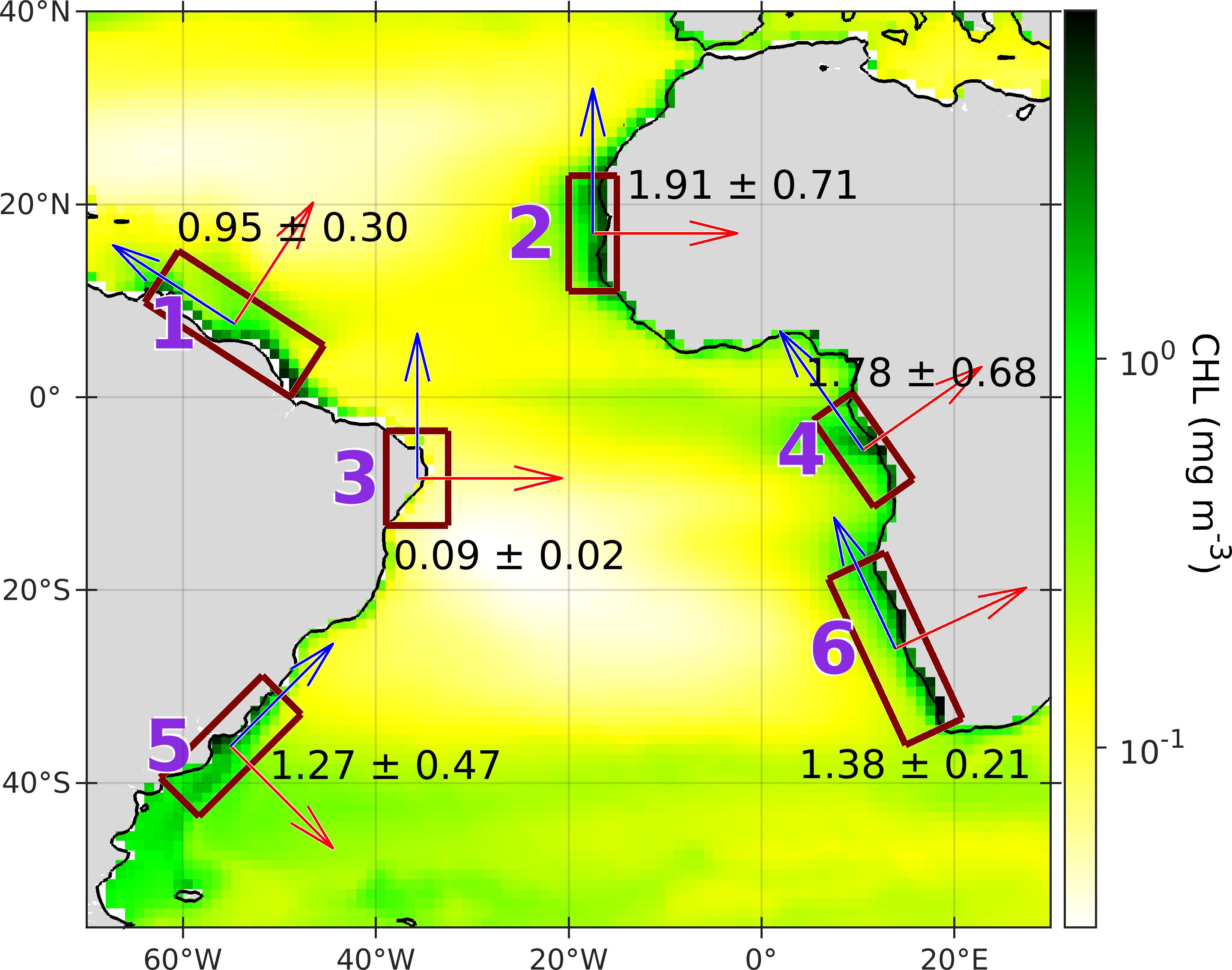
Figure 1. Definition of the six coastal regions (labeled by purple numbers) at the tropical and south Atlantic analyzed in this paper. Background color corresponds to the long-term mean of satellite-derived chlorophyll-a (CHL) for the 1998–2021 period. Mean ± standard deviation of spatially-averaged CHL are shown for each region. Vectors indicate the along-shore (blue) and cross-shore (red) directions in each region.

2.2 Analytical approach

In each region, monthly mean time series of spatially-averaged satellite-derived CHL is correlated with 1) 23 spatially-averaged physical variables obtained from oceanic and atmospheric gridded products (Table 1), 2) 14 teleconnection climatic indices (Table 2), to elucidate the physical drivers of the regional biogeochemical characteristics. The analysis period is from January 1998 to December 2021 (24 years). A monthly climatology (1998–2021 period) was subtracted from each data series to produce monthly anomalies and hence focus on interannual variations.

Table 1

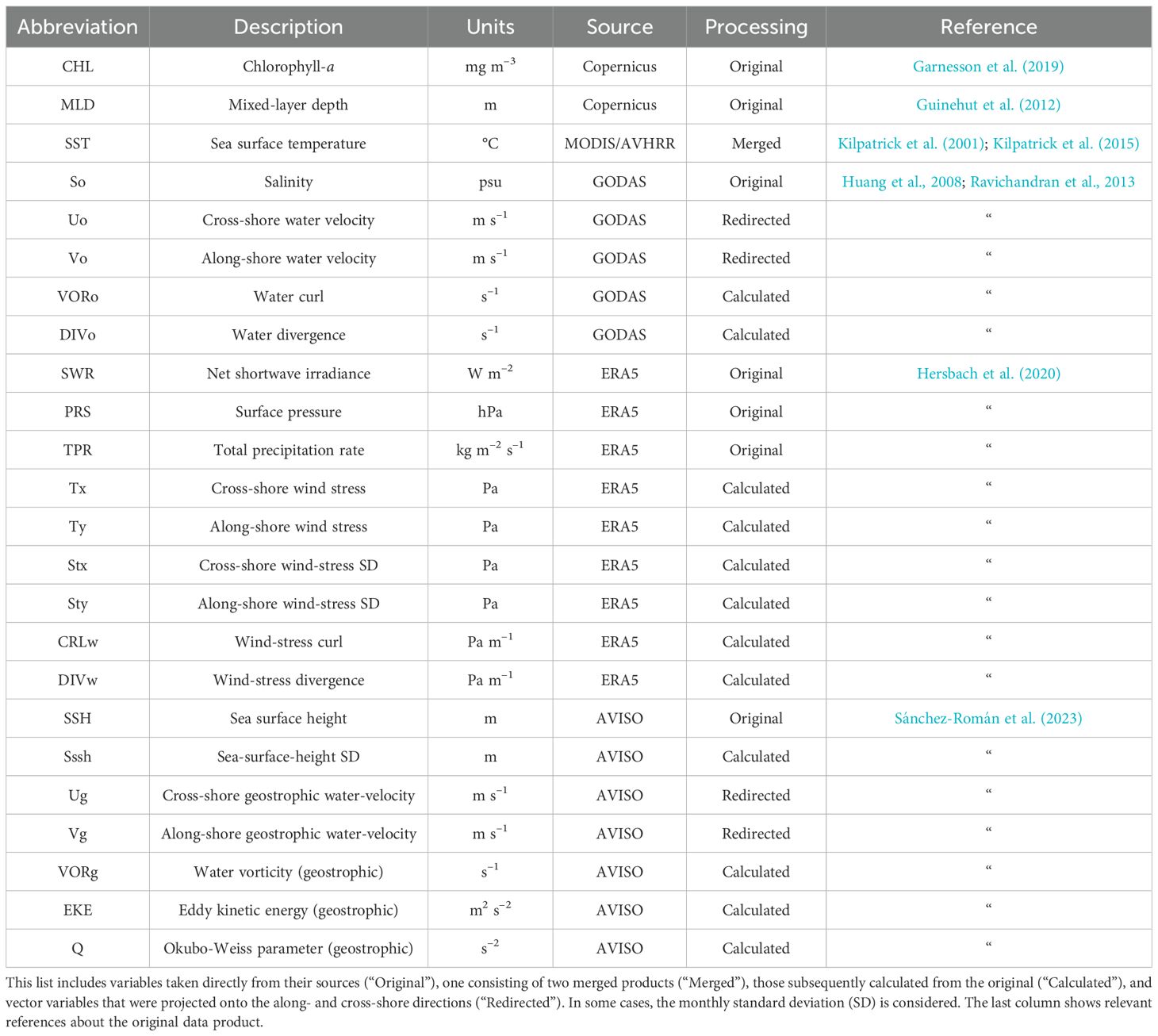
Table 1. Oceanographic variables included in the analysis (Section 2.2).

Table 2

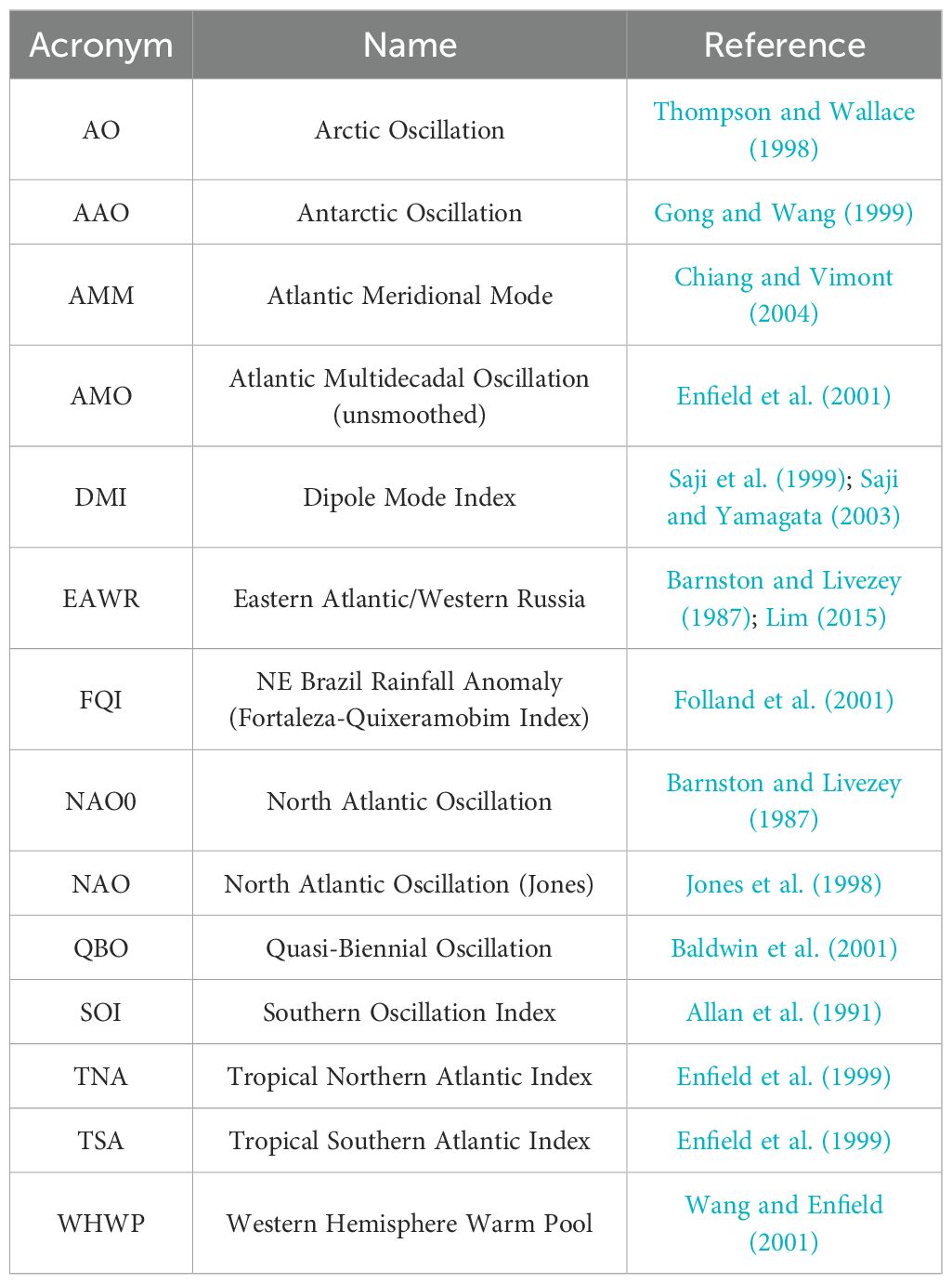
Table 2. Climate indices included in the analysis (Section 2.2) and relevant references.

The selected CHL dataset is a Level-4 gridded product by Copernicus Marine Environmental Monitoring Service (CMEMS, https://marine.copernicus.eu/). The other oceanographic variables were taken from different data sources, some of them taken directly from the source while the other resulted from a post-processing carried out for this analysis (Table 1). The large-scale teleconnection indices were mostly provided by the National Oceanic and Atmospheric Administration (NOAA) - Physical Science Laboratory (PSL; https://psl.noaa.gov/data/climateindices/list/); only those indices directly associated with, or with known effects on, the Atlantic were selected. For details about all these variables and indices, see Supplementary Section S1.

Then, in order to identify the dynamical factors that affect the CHL variability, a mechanistic-oriented correlation analysis was carried out for each region (for details, see Supplementary Section S2). This analysis consisted of 3 steps (Figure 2A): 1) correlating the CHL series whith those of the potential drivers, either the oceanographic variables (Table 1) with lag = 0 or the teleconnection indices (Table 2) with $0\le \text{lag}\le 9$ months; 2) ranking the significantly-correlated $(p<0.05)$ drivers’ series according to the magnitude (absolute value) of their correlations; 3) selecting the ranked drivers’ series with no covariability between each other. This selection (Step 3) is carried out by a cross-correlation of the ranked drivers’ series (from Step 2), reducing the number of independent drivers’ series (Figure 2B). The selected drivers’ series are the focus of our mechanistic analysis and are used as predictors to reconstruct the CHL (Section 2.3).

Figure 2

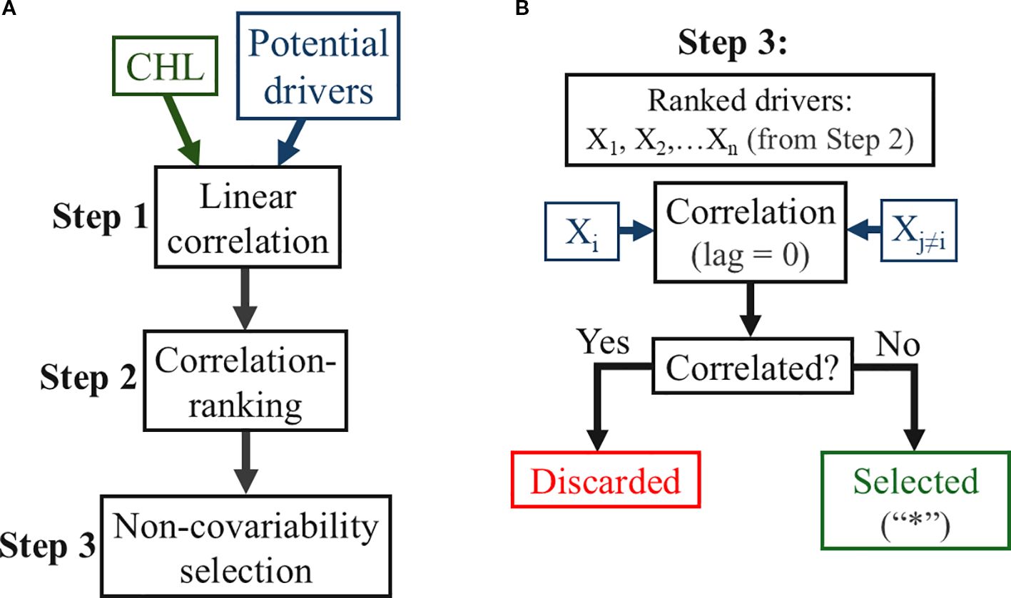
Figure 2. Schematics of the mechanistic-oriented correlation analysis applied in each of the study regions (Figure 1). (A) The regional CHL and the potential drivers are analyzed through 3 subsequent steps. Step 1: the drivers’ series are correlated with the CHL (with lag = 0 for the oceanographic variables; with 0 ≤ lag ≤ 9 months for the teleconnection indices, where the drivers lead the CHL); Step 2: the significantly-correlated (p < 0.05) drivers are ranked according to the absolute-value of their correlation; Step 3: from the ranked drivers, those with no significant correlation between each other are selected for subsequent analysis. (B) Selection process in Step 3: from top to bottom, the ranked drivers (X₁, X₂,…, X_n, where n is the number of significantly-correlated drivers) are correlated (lag = 0) between each other (r = corr (X_i, X_j≠i)), if the correlation (r) is significant the driver (X_j≠i) is discarded, otherwise the driver is marked as selected (labeled with asterisks in Figures 3, 4).

To elucidate the link between the oceanographic variables and the teleconnection indices, i.e. the large-scale dynamical patterns associated with each index, regression maps of the oceanographic variables were calculated as functions of individual climate indices. In preparation for these regression maps, each index was standardized (1998–2021 period), i.e. its mean was subtracted and the result was divided by its standard deviation, to ensure a mean of zero and for not dealing with the indices’ units. Then, a no-intercept linear regression-model was fitted (by a least-square technique) to every point of each variable’s gridded anomaly (1998–2021 period) as function of each standardized climate index; the regression map consists of the fitted coefficients.

2.3 Reconstruction of regional CHL series

Given the relatively short temporal coverage of the CHL datasets, barely long enough for interannual- but insufficient for decadal-variability analyses, it is desirable to extend its temporal extension. Then, herein we implement empirical models to estimate the CHL in each region (Figure 1) using the selected drivers’ series (Section 2.2) as predictors. These models consisted of three multi-linear regressions (Supplementary Section S3.1) and a non-linear approach based on artificial neural networks (Supplementary Section S3.2), defined as follows.

1. Regression of oceanographic variables: Includes the oceanographic fields (Table 1) resulting from the correlation analysis (Figure 2).

2. Regression of teleconnection indices: Includes the climate teleconnection indices (Table 2) resulting from the correlation analysis (Figure 2).

3. Regression of SST EOF modes: Includes the SST principal components (eigen-value series) taken from the first 27 EOF modes of an extended SST product (Supplementary Section S1.3).

4. Neural network model: Includes the selected oceanographic variables (as in the first regression model), based on nonlinear autoregressive networks with exogenous inputs (NARX).

For details about the models, see Supplementary Section S3.

3 Results

3.1 Regional drivers

3.1.1 Region 1: North Brazil Current

In this region, the CHL is significantly correlated with 15 out of the 23 oceanographic variables, but only three show no covariability between each other (Figure 3): sea-surface height (SSH) $(r=0.33),$ total precipitation rate (TPR) $(r=0.24)$ and SSH standard deviation, SD (Sssh) $(r=-0.13)$. The oceanographic variables that explain the regional CHL are in turn explained by large-scale oceanic and atmospheric patterns, that link the regional climatic conditions to those in adjacent and/or remote locations. Some of these climatic patterns are represented by teleconnection indices like the ones described in Section 2.2 and Table 2. The CHL is significantly correlated with 7 out of the 14 indices, but only three show no covariability between each other (Figure 4): Tropical Southern Atlantic (TSA) ($r=0.31$, lag = 5 months), Southern Oscillation Index (SOI) ($r=0.26$, lag = 1 month), and Eastern Atlantic/Western Russia (EAWR) ($r=-0.12$, lag = 4 months).

Figure 3

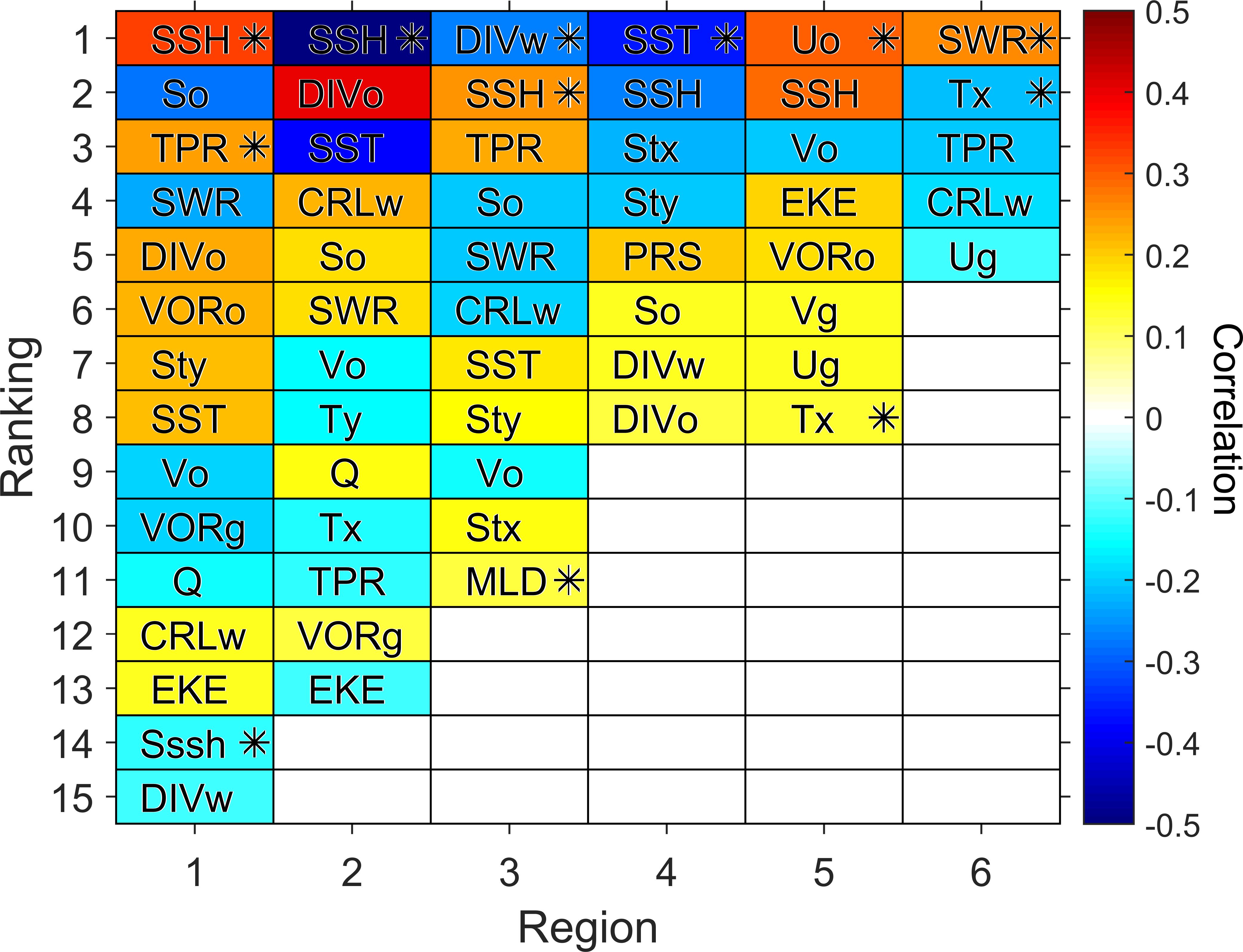
Figure 3. Oceanographic variables (from those in Table 1) significantly correlated (p < 0.05) with the satellite-derived CHL at each of the regions defined in Figure 1, ranked by the absolute value of their correlation for the 1998–2021 period (the highest values at the top). Color corresponds to zero-lag correlation. The asterisks indicate the most correlated variables showing no covariability between each other (Figure 2).

Figure 4

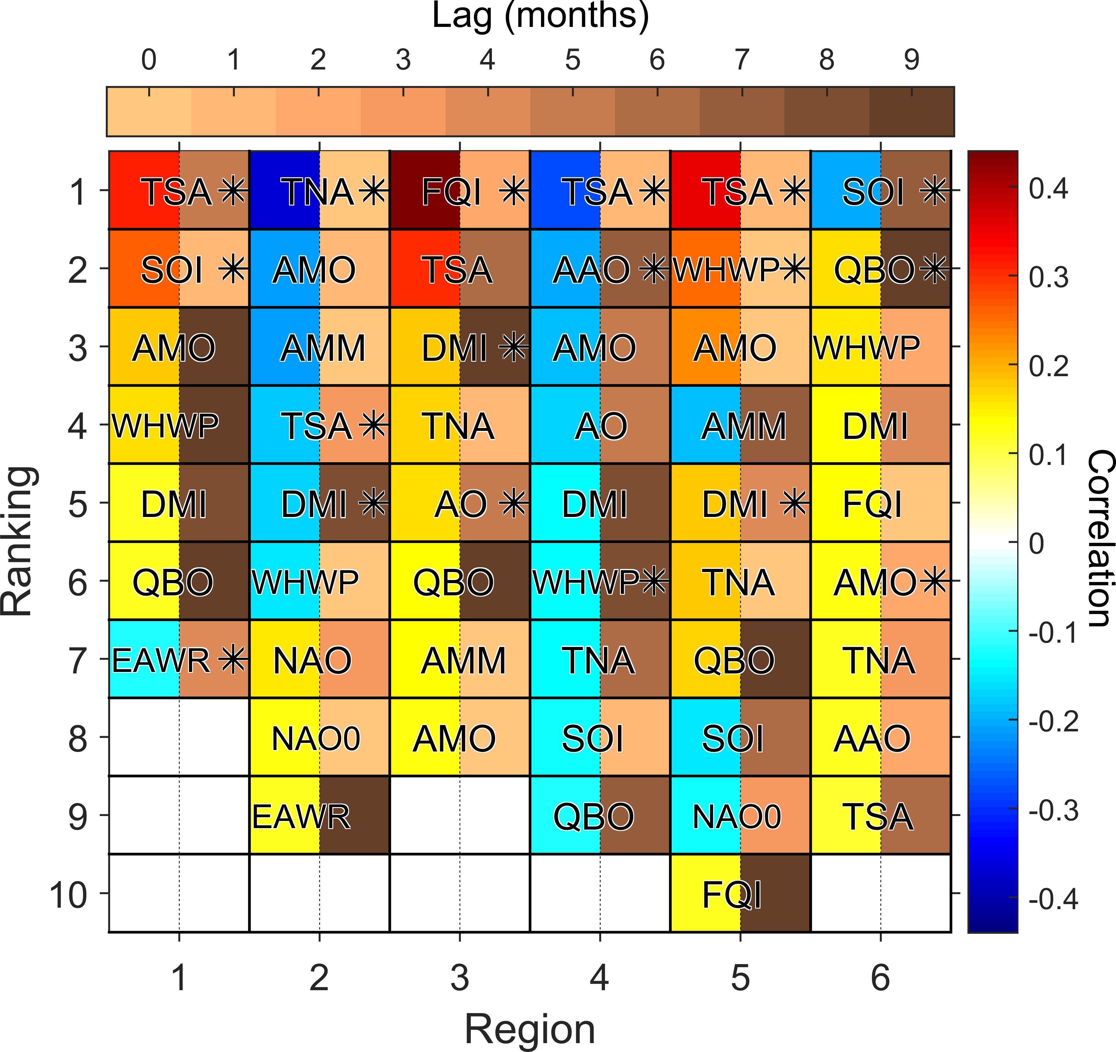
Figure 4. Teleconnection indices (from those in Table 2) significantly correlated (p < 0.05) with the satellite-derived CHL at each of the regions defined in Figure 1, ranked by the absolute value of their correlation for the 1998–2021 period. In each case, both the correlation (blue-to-red) and the lag (beige-to-brown) are indicated. The asterisks indicate the most correlated (lagged) indices showing no covariability between each other (Figure 2).

The TSA (Enfield et al., 1999) is characterized by an equatorial warming that induces a weakening of the North Brazil Current (NBC) and the NBC retroflection (Figure 5a), and of the trade winds (Figure 5b), which affect the regional flows as corroborated by its correlation (same lag of 5 months) with SSH (r = 0.21) and Sssh (r = −0.19). The TSA also induces a positive precipitation anomaly over the region (Figure 5c), hence its correlation (same lag) with TPR (r = 0.15), resulting in a freshwater anomaly enhanced by an increased flow of the Amazon River. The SOI (e.g., Allan et al., 1991), whose positive values correspond to La Niña (cold episodes) and the negative to El Niño (warm episodes), is associated with a roughly coherent intensification of the NBC and the NBC retroflection (Figure 6a), anomalous shoreward winds (Figure 6b). and increased precipitation near the Equator (Figure 6c) presenting a correlation with TPR (r = 0.22). The EAWR (Barnston and Livezey, 1987; Lim, 2015) is associated with a weak variability in the NBC and a weak precipitation decrease (not shown), showing no correlation with the three selected oceanographic variables.

Figure 5

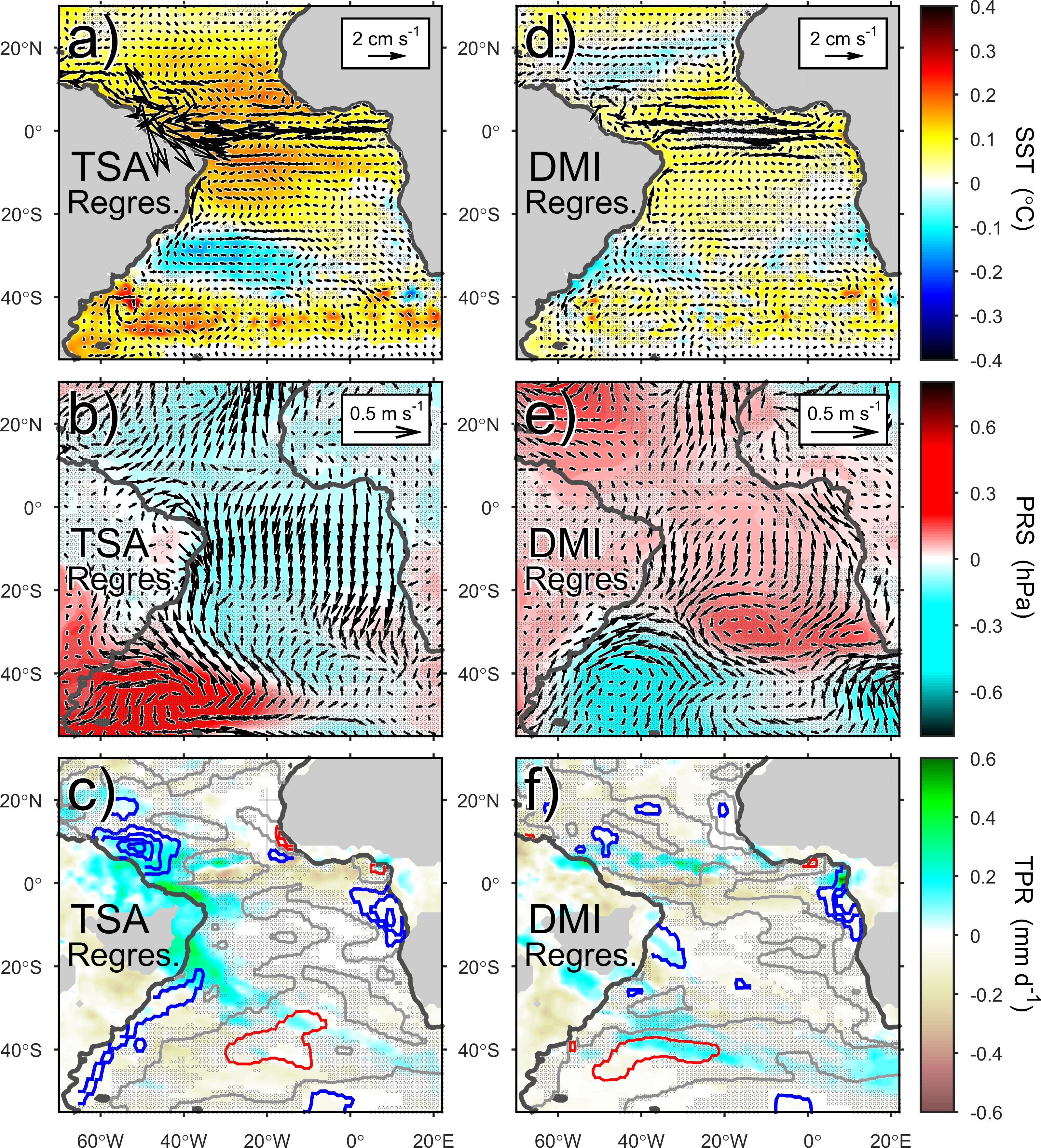
Figure 5. Regression of oceanographic anomalies onto (a–c) the Tropical Southern Atlantic index (TSA) and (d–f) the Dipole-Mode index (DMI) for the 1998–2021 period. These leading indices have lags of 2 and 7 months, respectively. (a, d) SST and surface-current vectors; (b, e) sea-level pressure and wind vectors; (c, f) precipitation rate and salinity contours (intervals of 0.03; red are positive, blue are negative, gray are zero). Shadded areas indicate that at least one of the plotted variables is not significant (95% confidence interval).

Figure 6

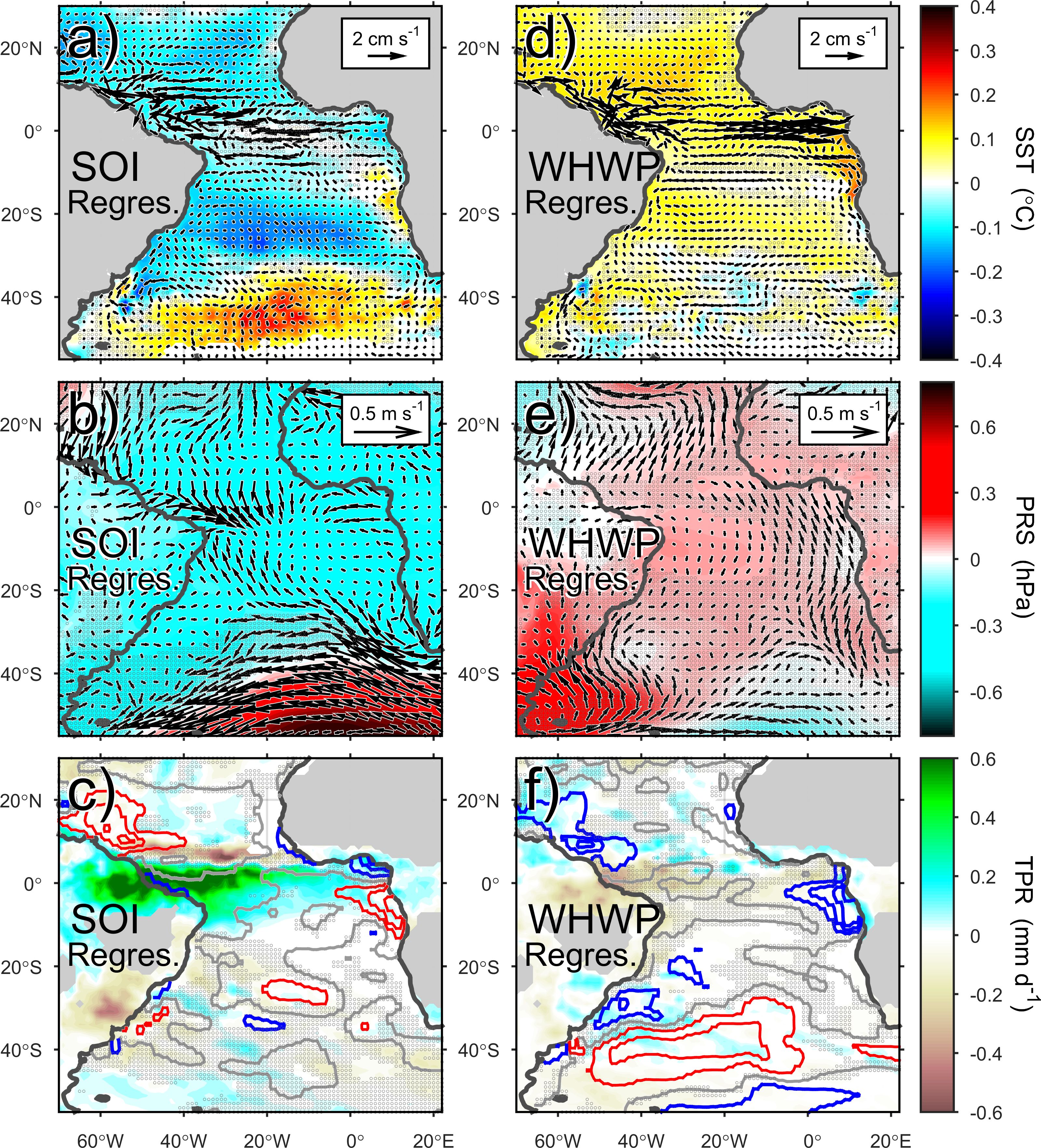
Figure 6. Same as Figure 5, but for (a–c) the Southern Oscillation Index (SOI) and (d–f) the Western Hemisphere Warm Pool index (WHWP). These leading indices have lags of 5 and 4 months, respectively.

3.1.2 Region 2: Mauritania-Senegal

In this region, the CHL is significantly correlated with 13 oceanographic variables, but all of them show some covariability with the selected, top correlated variable (Figure 3): SSH (r = −0.50). The teleconnection indices that independently (between each other) explain the most CHL variability are Tropical Northern Atlantic (TNA) (r = −0.37, lag = 0), TSA (r = −0.18, lag = 3 months) and Dipole Mode Index (DMI) (r = −0.17, lag = 8 months), as shown in Figure 4.

The TNA (Enfield et al., 1999) is associated with a weakening of the trade winds which results in a weaker upwelling on the northern portion of the region (not shown); these effects are evident in the significant TNA-SSH correlation (r = 0.39). The TSA has a weakening effect on the trade winds and the upwelling-favorable winds on the northern portion of the region (Figure 5b), similar to that of the TNA, but resulting in a lower correlation with SSH (r = 0.29). On the other hand, the DMI (Saji et al., 1999; Saji and Yamagata, 2003) causes equatorward near-coastal flows (Figure 5d) and a weakening of the upwelling-favorable winds (Figure 5e); this index shows no significant correlation with SSH.

3.1.3 Region 3: Eastern Brazil

This region, herein considered as a counterpart analogous to Region 4 described in the next section, is characterized by remarkably lower CHL values, but is an important dynamical region in the western Atlantic. In this case the non-covariability variables correlated with CHL are wind-stress divergence (DIVw) (r = −0.27), SSH (r = 0.25) and mixed-layer depth (MLD) (r = 0.12), as shown in Figure 3. In this region the selected climate indices are Fortaleza-Quixeramobim Index (FQI) (r = 0.44, lag = 2 months), DMI (r = 0.18, lag = 9 months), and Arctic Oscillation (AO) (r = 0.16, lag = 5 months), as shown in Figure 4.

The FQI is especially adequate for this region, as expected because it is calculated with two locations at Northeastern Brazil, and it indeed shows the strongest correlation in the ranking for all the regions. FQI is associated with increased precipitation and southward-wind anomalies over this region (not shown), which indicates that this region’s CHL is modulated by displacements of the intertropical convergence zone (ITCZ). The DMI induces weak variability on the surface circulation (Figure 5d), southward winds (Figure 5e) and weak negative precipitation-anomalies (Figure 5f). The AO (Thompson and Wallace, 1998) has effects similar to those of the DMI mentioned above but weaker (not shown). In this region, none of the selected indices is correlated with any of the selected oceanographic variables.

3.1.4 Region 4: Gabon-Congo-Angola

This region is part of the tropical Angolan upwelling system (e.g., Imbol Koungue et al., 2024), hence its driver-linked variables are mostly upwelling-related. As in Region 2, only one variable is selected as the best predictor but it is SST (r = −0.36) instead of SSH (Figure 3). This region’s leading indices are TSA (r = −0.28, lag = 1 month), Antarctic Oscillation (AAO) (r = −0.20, lag = 7 months), and Western Hemisphere Warm Pool (WHWP) (r = −0.14, lag = 8 months).

The TSA induces a weak warming (Figure 5a), evidenced by its correlation with SST (r = 0.48), and an apparent weakening of the South Atlantic Anticyclone, this anomaly’s outer edge causes southward winds (weakened upwelling) over the region (Figure 5b). This index also shows a negative salinity anomaly (Figure 5c) associated with increased flow of the Congo River. The AAO (Gong and Wang, 1999) is associated with a precipitation increase over this region and a reduction in the salinity (not shown), also attributable to an enhanced Congo riverine input. The WHWP (Wang and Enfield, 2001) induces a warming, hence its correlation with SST (r = 0.16), and a weakening of the equatorward flow (Figure 6d), as well as anomalously-poleward winds (Figure 6e), and a moderate excess precipitation and enhanced riverine input (Figure 6f). Notice that even though these WHWP-induced anomalies might not entirely satisfy our significance criterion, the coherent distribution of the wind vectors and the sea-level pressure (SLP) contours, together with the agreement between these two fields (Figure 6e), reinforces our confidence on the plotted results.

3.1.5 Region 5: Brazil-Uruguay-Argentina

CHL in this region is mostly explained by cross-shore water velocity (Uo) (r = 0.30) and cross-shore wind stress (Tx) (r = 0.13) (Figure 3). The selected climate indices that most explain the regional CHL are TSA (r = 0.35, lag = 1 month), WHWP (r = 0.25, lag = 0), and DMI (r = 0.18, lag = 4 months) (Figure 4).

The TSA induces a warming and anticyclonic anomaly at the Region’s central portion (Figure 5a) barely reflected in its correlation with Uo (r = 0.14) and which has a weakening effect on the Malvinas Current (MC), strong onshore/poleward winds driven by an anticyclonic circulation associated with an intense high-pressure anomaly (Figure 5b), and a freshwater anomaly (Figure 5c) most probably associated with increased flow of the La Plata River. The WHWP causes a modest weakening of the MC (Figure 6d), somewhat linked with its correlation with Uo (r = 0.22), anomalous shoreward winds (Figure 6e), and a moderate excess precipitation and enhanced riverine input in the Region’s northern portion (Figure 6f). The DMI causes a weak cooling and some intensification of the poleward flow associated with the Brazil Current (BC) (Figure 5d), strong equatorward winds driven by a low-pressure anomaly off this region (Figure 5e), and a near-coastal increase of the freshwater input (Figure 5f).

3.1.6 Region 6: Namibia-South Africa

Although this region is part of the Benguela Current System, in terms of interannual variability the upwelling plays a minor role to explain the regional CHL. Solar light is the most important driver, represented by shortwave irradiance (SWR) (r = 0.26), followed by the cross-shore winds, represented by cross-shore wind-stress (Tx) (r = −0.21) (Figure 3). The teleconnection indices that most explain this region’s CHL are SOI (r = −0.20, lag = 7 months), Quasi-Biennal Oscillation (QBO) (r = 0.16, lag = 9 months) and Atlantic Multidecadal Oscillation (AMO) (r = 0.13, lag = 2 months) (Figure 4).

The SOI is associated with a warming and a cooling in this region’s northern and southern half, respectively, together with a cyclonic circulation in its southern part that induces an anomalous poleward flow in the Region’s southern half (Figure 6a), and SOI also shows poleward wind anomalies over the whole region (Figure 6b). The QBO (Baldwin et al., 2001) is associated with modest warming and intensification of the equatorward near-coastal flow (induced by an anticyclonic gyre) in the southern portion of the region, and a weak intensification of upwelling-favorable winds over all the region (not shown). This index shows some correlation with SWR (r = 0.16), consistent with the notion of the relation between the mesoscale flow and cloudiness. The AMO (e.g., Enfield et al., 2001) is associated with weak flow intensification a marked weakening of the upwelling-favorable winds, and an anticyclonic wind curl over Cape Agulhas (not shown).

3.2 Reconstruction of regional CHL

3.2.1 Fitting/training 1998–2021 period

In the previous section we identify the oceanographic variables and climate indices that explain the CHL in the analyzed regions. Based on these results, herein we present four different approaches to reconstruct the regional CHL series (Section 2.3), which are potentially useful to extend the CHL estimates to periods when CHL satellite observations are not available. Figure 7 shows a comparison between the satellite-derived CHL and the CHL-reconstruction models for each analyzed region, and the corresponding statistical results are shown in Table 3. RMS errors are normalized by the SD of the satellite-derived CHL for better comparison among the differently-productive regions. In this section we focus on the 1998–2021 period (shaded area in Figure 7), in which the models’ linear coefficients were calculated (Supplementary Section S3.1) and the training of the neural network was carried out (Supplementary Section S3.2).

Figure 7

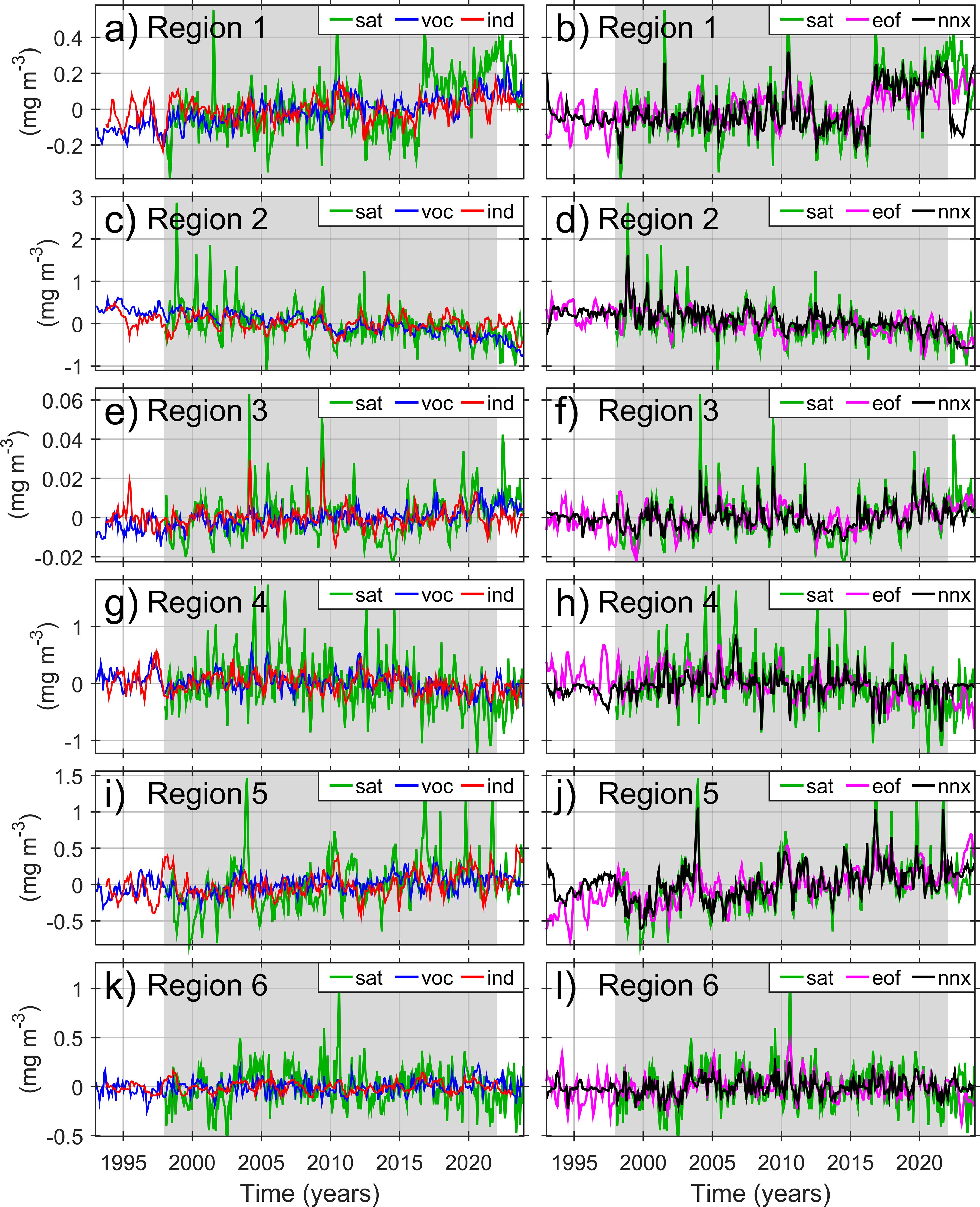
Figure 7. (a–l) Comparison between the regional satellite-derived CHL (“sat”, green line) and CHL-reconstruction models (Section 2.3), in mg m-3, in the six analyzed regions (ordered from top to bottom). These models include the multi-linear models using oceanographic variables (“voc”), climate indices (“ind”) and SST EOF modes (“eof”) (Supplementary Section S3.1), and the neural network model using the oceanographic variables as input data (“nnx”) (Supplementary Section S3.2). The CHL-reconstruction series (“voc”, “ind”, “eof”, “nnx”) cover a time-span from 1993 to 2023, while the satellite-CHL series (“sat”) extends from 1998. The shaded areas indicate the 1998–2021 period, used for the calculation of the coefficients involved in the multi-linear models and for the training of the neural-network model.

Table 3

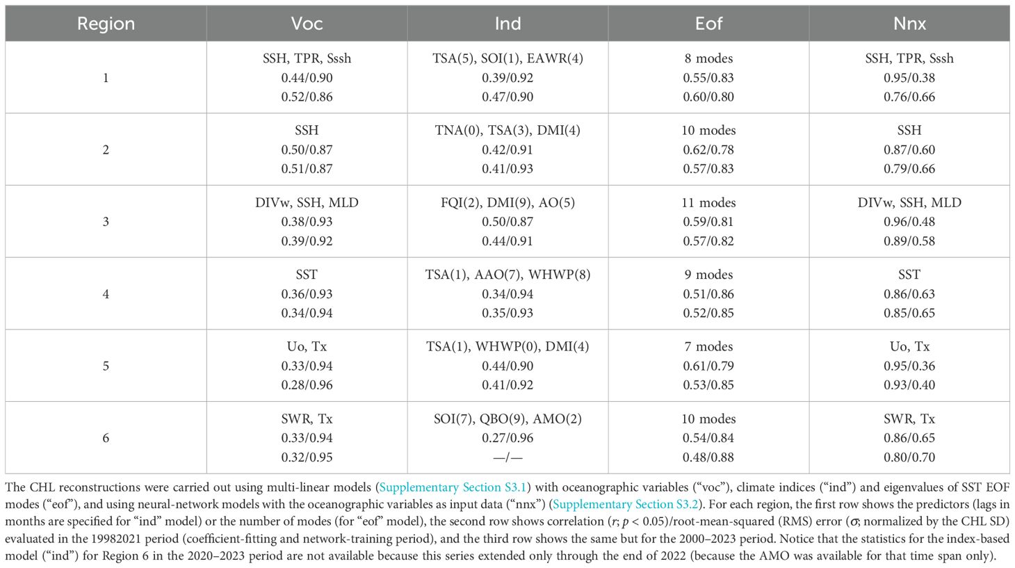
Table 3. Comparative results among the CHL-reconstruction models described in Section 2.3, with respect to the satellite-derived CHL, for the regions shown in Figure 1.

The first CHL-reconstruction approach is a multi-linear regression using oceanographic variables (Supplementary Section S3.1). Essentially, this approach takes the selected variables, i.e. those showing no covariability between each other, from the correlation ranking shown in Figure 3 as predictors to form a model for each region (no lag is applied to the series). This multilinear model captures much of the CHL variability, especially lower-frequency, but there are many CHL peaks that the model underestimates or is unable to reproduce (Figure 7, first column). The correlation range is 0.33-0.50 (Table 3); Region 2 shows the highest correlation (r = 0.50) with the smallest error (σ = 0.87) and Regions 5 and 6 show the lowest correlation (r = 0.33) with the largest error (σ = 0.94). As shown in Figure 3, Region 2 uses only one predictor (SSH), whereas two predictors are used each of Regions 5 (Uo and Tx) and 6 (SWR and Tx).

The second approach to reconstruct the regional CHL is also a multi-linear regression but using the teleconnection indices as predictors (Supplementary Section S3.1), using the selected indices shown in Figure 4 i.e. those with no covariability between each other, and considering the corresponding lags (Table 3). As in the previous case, this model captures much of the CHL variability (Figure 7, first column) but many peaks are underestimated or not reproduced. This index-based model shows no better results, compared to the previous model, in Regions 1, 2 and 6, but it is similar in Region 4 and even slightly better in Regions 3 and 5 (Table 3). Region 3 shows the highest correlation (r = 0.50) with the smallest error (σ = 0.87), and Region 6 shows the lowest correlation (r = 0.27) with the largest error (σ = 0.96).

The third CHL-reconstruction approach consisted also of a multi-linear regression but it uses the eigenvalues of SST EOF modes as predictor variables (Supplementary Section S3.1), using the selected modes and corresponding lags shown in Figure 8. The first 27 EOF modes are above the random confidence-level (Supplementary Section S1.3) and should be (in theory) physically meaningful and safe to use in our analysis. By definition, the EOF modes are linearly independent between each other and hence uncorrelated, but this not necessarily the case when lags are applied (Figure 8) on the eigenvalue series (principal components), hence a covariability-selection makes sense; therefore, the covariability among the lagged eigenvalue series was removed before using them in the model, similarly to the two previous multilinear models.

Figure 8

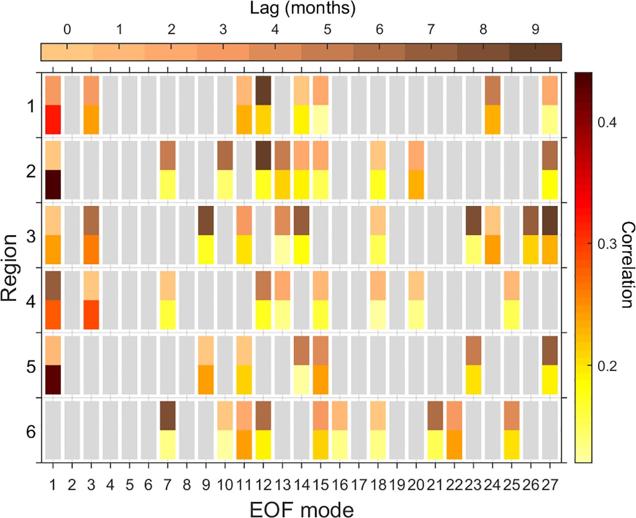
Figure 8. Tabular array indicating the SST EOF modes used in each region (Supplementary Section S3.1). Bars’ color indicates: correlation in the upper halves, the corresponding lag in the lower halves. Gray bars indicate insignificant correlations.

None of the EOF modes showed correlation with all the six regions, and seven (2, 4, 5, 6, 8, 17, 19) out of the 27 modes were not used in the regression model (Figure 8). Region 5 uses the lowest number of modes (7), while Region 3 uses the highest number (11). The EOF-based model is better to reproduce the regional CHL than the models described above (Figure 7, second column); indeed, the EOF-model’s lowest correlation (r = 0.51) is higher than the highest correlation obtained in the previous models, and the errors are smaller (Table 3). Region 2 shows the highest correlation (r = 0.62) with the lowest error (σ = 0.78), and Region 4 shows the lowest correlation (r = 0.51) with the largest error (σ = 0.86).

Finally, a highly non-linear approach is herein adopted to reconstruct the regional CHL, based on NARX (Supplementary Section S3.2). As the first multi-linear approach described above, this model uses the selected, non-covariability oceanographic variables ranked in Figure 3 as predictor variables. This NARX model is remarkably better than the previous models, closely reproducing most of the CHL variability (Figure 7, second column). The model shows correlations over 0.85 and errors under 0.70 (Table 3). Region 3 shows the best represented CHL (Figure 7f) with a nearly perfect correlation (r = 0.96) and a relatively-medium error (σ = 0.48). Regions 4 and 6 (Figures 7h, l) show the lowest correlation (r = 0.86) with the largest errors, but even these “poor” results are better than those from the multi-linear models.

3.2.2 Projection

The CHL reconstructions in the previous section can be used to project the estimated-CHL series either forward or backward in time beyond the fitting/training period (1998-2021), i.e., here we refer to “projection” as the CHL reconstruction beyond the period (1998-2021) that was used for model training. The projections were performed for the 1993–1997 and 2022–2023 periods (Figure 7). However, there are no satellite-CHL data in the 1993–1997 period to evaluate the projection skill. The 2022–2023 period is too short for a statistical comparison consistent with that carried out for the 1998–2021 period, therefore, we decided to use a period of a similar length which includes that period, 2020-2023, and focus on how much the correlations and errors change with respect to those calculated for the 1998–2021 period; these results are also shown in Table 3. The results are similar between both evaluation periods in the model based on oceanographic variables (“voc”), while the results tend to be slightly worse in the index-based model (“ind”), the EOF-based model (“eof”) and especially in the neural-network model, in the projection period (2000-2023). This evaluation is not very sensitive but the series shown in Figure 7 are helpful to corroborate the correlation/error results. The “voc” model is indeed slightly closer to the satellite CHL than the other models, followed by the “eof”; the last years in Region 1’s series are especially problematic for the models, the “nnx” model even shows an abrupt fall right after the projection starts, an apparent unconstrained non-linear response of the model. On the other hand, there are marked differences among the models in the initial 1993–1997 period (Figure 7), when CHL is not available for comparison. In this case, the “nnx” seems to be too different with respect the other models and hence its projection skill is questionable. There is some consistency among the multi-linear models to reproduce some peaks, especially in Region 4 where there is a remarkable agreement between the “voc” and the “ind”. All these results suggest that the CHL can be reasonably projected at least through 2–5 years beyond the fitting period, but using multi-linear models, in particular with the “voc” model.

4 Discussion

4.1 Drivers of chlorophyll-a variabilty

Our comprehensive analysis of observational data has allowed the identification of many of the physical drivers for the CHL in the six analyzed regions, as well as the teleconnection patterns involved in the large-scale patterns. Figure 9 shows a summary of these main results of our analysis. The analyzed regions are characterized by a vigorous interannual variability; comparing the regional CHL SD before (Figure 1) and after removing the monthly climatology (Figure 9) indicates that the interannual variability has roughly half of the amplitude of the mean seasonal cycle in the tropical regions (1 to 4), but they are comparable in the southernmost regions (5 and 6). This interannual variability is a result from different drivers, herein represented by those oceanographic variables that explain a significant fraction of the observed CHL variability.

Figure 9

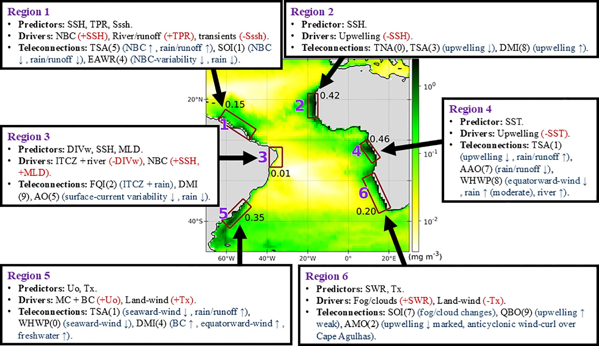
Figure 9. Summary of the main results (predictor variables, physical drivers, teleconnection patterns) for each of the six analyzed regions. The predictors and indices correspond to the non-covariability selections described in Section 3.1; numbers in parentheses correspond to their lags in months. Vertical arrows indicate intensification (↑) or weakening (↓) of the specified process. Signs of the drivers’ predictor variables match their correlation signs in Figure 3. Background color corresponds to the standard deviation of satellite-derived chlorophyll-a (CHL) for the 1998–2021 period, after removing the monthly climatology for the same period. Spatially-averaged values are shown for each region.

In Region 1, SSH and Sssh are variables which can serve as proxies for the regional surface circulations, the North Brazil Current (NBC) (Johns et al., 1998; Vallès-Casanova et al., 2022), the NBC retroflection (Johns et al., 1990; Richardson et al., 1994), and the anticyclonic rings that are shed from it (Richardson et al., 1994; Fratantoni and Glickson, 2002; Bueno et al., 2022; Garzoli et al., 2003) that can interact with other eddies (Subirade et al., 2023). Surface mean circulation is responsible for horizontal export of nutrients (Santos et al., 2008), while eddy features can have different local effects on the CHL (e.g., Pereira et al., 2019). These effects are caused by eddy-wind driven upwelling, vertically transporting nutrients to the surface levels and hence modifying the phytoplankton growth (McGillicuddy et al., 2007; Pereira et al., 2019), or by eddy-interactions which can modify the biogeochemical properties of the water column and shape the CHL distribution (Hernández-Carrasco et al., 2020). Other transient motions like coastal-trapped waves (CTW), both intraseasonal (Imbol Koungue and Brandt, 2021) and interannual (Bachèlery et al., 2020), would affect the local phytoplankton growth. This effect can be by upward nitrate flux induced by nitrocline displacements combined with intense vertical mixing (Körner et al., 2024), or by enhanced CTW-induced along shelf flows (e.g., Rivas, 2017) that might export nutrients and CHL to other zones. Also, the wind fluctuations that generate the CTW might have an enhancing effect of surface seawater turbulence favorable to the phytoplankton (e.g., by turbulent supply of nutrients; Hales et al., 2009). Precipitation rate (TPR) can impact CHL (r = −0.21) through modification of the freshwater input and runoff from land. This runoff carries a large amount of nutrients essential for phytoplankton growth (Santos et al., 2008), and also an important amount of suspended particles that limit the incoming light necessary for the phytoplankton (DeMaster et al., 1986), in addition to the SWR reduced by the prevalent cloudiness that comes with precipitation (e.g., McQuate and Hayden, 1984; Chaves and Cavalcanti, 2001; Yan, 2005).

In Region 2, which is part of the four major Eastern Boundary Upwelling Systems (e.g., Quiñones, 2010), the wind-driven offshore Ekman transport generates a divergence over the shelf (e.g., Trautman and Walter, 2021) and a sea-level decrease near the coast (e.g., Kruse and Huyer, 1983) while cold and saltier water from deeper levels compensates the offshore transport. Dynamical features linked to the upwelling front, like an equatorward alongshore flow (e.g., Allen, 1973) would affect the nutrient distribution, and the mesoscale structures shed from it can increase the CHL (e.g., Hernández-Hernández et al., 2020), especially the cyclonic structures due to a shoaling of the isopycnals and the nitrocline (e.g., Hernández-Hernández et al., 2020), and hence the subsurface chlorophyll-a maximum (e.g., Almazán-Becerril et al., 2012). Rainfall events can interact with upwelling intrusions to produce temporal variations in phytoplankton biomass (Valentin et al., 2021), and cross-shore winds can induce a flux of nutrients and micronutrients from the Saharan desert (Mills et al., 2004; Mahowald et al., 2009; Shi et al., 2022), modulated by the passage of African easterly waves (Bloomfield et al., 2022; Nakamae and Shiotani, 2013).

In Region 3, the atmospheric circulation is influenced by the ITCZ (e.g., De Albuquerque Cavalcanti, 2015) which modulates the wind field, rainfall and solar radiation thus affecting the regional phytoplankton growth. SSH is a proxy for the driving effect by the NBC and the North Brazil Undercurrent (Dossa et al., 2021), together with a weak influence of the Amazon River and the Saõ Francisco River (Rodrigues Holanda et al., 2021).

In Region 4, SST is linked to atmopsheric patterns like the ITCZ which creates strong convective activity, characterized by atmospheric-pressure reductions and wind convergence at surface that generates the thunderstorms that characterize the tropical regions (Huntley, 2019). These storms can lead to a deepening of the mixed-layer depth and a dilution of the deep chlorophyll-a maximum (Barrillon et al., 2023).

In Region 5, cross-shore velocity Uo represents the circulation variability dominated by the Malvinas Current (MC) in the south and the Brazil Current (BC) in the north, which converge near 34^°S (Piola et al., 2018; Artana et al., 2021), and the mesoscale dynamics enhanced as a consequence of the MC-BC interation (+EKE, +CHL) (as in Frey and Kubryakov, 2023). These hydrodynamic features have an influence on the regional transport of nutrients, especially those originated in the La Plata River’s plume and the lagoon systems (Niencheski, 2018). Tx represents the variability of cross-shore winds, responsible for an atmospheric input of limiting micro-nutrients (i.e., iron) from land, mostly from the Patagonian desert (Johnson et al., 2010), and which are driven by the winds associated to high and low pressure systems characteristic of South Brazil and the nearly-weekly southwesterly cold fronts (Rodrigues et al., 2004; Wahrlich et al., 2018).

In Region 6, shortwave-irradiance SWR variability is driven by the characteristic fog and low-level clouds in the Namib area (Andersen et al., 2019, 2020), and this cloudiness would produce some precipitation. Tx represents the cross-shore winds which plays an important role transporting nutrients from desert areas to the ocean surface, in the form of dust plumes linked to salt pans and dry river valleys in the Namib desert (Eckardt and Kuring, 2005). Windblown dust within the river valleys is easily transportable offshore from the Namib over the Benguela Upwelling System (Dansie et al., 2017c), containing great concentrations of bioavailable iron and enriched nitrogen and phosphorus, which may positively impact marine productivity in the southern Atlantic (Dansie et al., 2017a, b).

SST anomalies in the tropical Atlantic (TSA and TNA; Figures 5a–c) have a marked effect on the rainfall over northeastern Brazil (and the Amazon basin) through the modulation of the latitudinal position of the ITCZ (Nobre and Shukla, 1996; Hounsou-Gbo et al., 2019). The El Niño Southern Oscillation (ENSO) also has a significant effect on the rainfall in the western near-equatorial Atlantic; along the ENSO cycle (Figures 6a–c but for SOI < 0), the ascendant branch of the Pacific Walker cell shifts to the east and the Pacific-Atlantic cell shows enhanced subsidence over equatorial South America and the western Atlantic, causing a more stable atmosphere which reduces the moist convection (Rodriguez-Fonseca et al., 2023). Marine resources in the northwest African coast are well affected by the ENSO variability, for example, the El Niño has been used as a predictor of the sardinella population biomass and distribution in the central-southern portion of the Canary Current Upwelling System (López-Parages et al., 2020).

The eastern Atlantic off Mauritania exhibits intense SST interannual varability associated with the Dakar Niño/Niña involving ocean-land-atmosphere coupled processes (Oettli et al., 2016; Koseki et al., 2024), which would have their signature in variables like SSH and others (consistent with the ranked variables in Figure 3). On the eastern tropical Atlantic, positive Dipole Mode Index (DMI) episodes (Figures 5d–f) drive tropospheric circulation changes that lead to an increase in moisture convergence and convection over the Congo basin and an increase in Congo River discharge (Jarugula and McPhaden, 2023), as evidenced in the reduced salinity in that region (Figure 5f). In the western south Atlantic, salinity and CHL anomalies show significant correlation with the Atlantic Multidecadal Oscillation (AMO) (Pacheco et al., 2022), apparently associated with an onshore advection of moist and relatively-warm air.

On the other hand, winds are responsible for upper-ocean nutrient-enrichment processes like coastal upwelling, a determinant factor for phytoplankton growth, and their changes can modify the spatial distribution (and even stability) of the upper-ocean circulation, and hence affect the transports of nutrients and phytoplankton. The wind-field patterns can be also modified by large-scale teleconnection mechanisms. For example, near-equatorial warmings (TSA and TNA) produce a weakening of the trade winds (Nobre and Shukla, 1996; Hounsou-Gbo et al., 2019) (Figure 5b). Also, there is a weak but significant correlation between the ENSO and the Brazil Current (BC) SST (with an 8-month lag when ENSO leads) in austral summer, linked to changes in upwelling-favorable winds and the intensity of the trade winds, associated with changes of the South Atlantic anticyclone intensity and position (Rouault and Tomety, 2022). The ENSO also induces a subsidence over the equatorial western Atlantic, which produces a weakening of the trade winds (Figure 6b for SOI < 0) and a reduction of the upwelling in that area (Rodriguez-Fonseca et al., 2023). These wind-field variations, specifically the wind-stress curl (Fonseca et al., 2004), have a modification effect on the surface equatorial currents (Figures 5a, 6a); the North Brazil Current (NBC) also presents a multidecadal variability (Tretkoff, 2011). Detachment of anticyclonic eddies from the NBC retroflection occurs during periods when this retroflection is weakened (Didden and Schott, 1993), but these eddies’ formation mechanism has been associated with short equatorial Rossby waves, generated by wind variations in the tropical Atlantic (Ma, 1996). The detached eddies can interact with the Amazon River plume, resulting in a CHL increase (Fratantoni and Glickson, 2002), and responsible for the transport of water properties to the northwest (Richardson et al., 1994; Fratantoni and Richardson, 2006).

South of the tropical band, the BC transport is significantly correlated with the sea-level pressure (Schmid and Majumder, 2018) and the wind-stress curl in the western Atlantic (Goes et al., 2019) (Figures 5b, e, 6b–e). The BC transport is also correlated with the ENSO and teleconnection indices not considered in our analysis (namely, the South Atlantic Subtropical Dipole Mode and the Southern Annular Mode) (Schmid and Majumder, 2018). These BC’s variations must modulate the formation of eddies in the Brazil-Malvinas confluence zone (Frey and Kubryakov, 2023), which can be detected by their enhanced CHL levels (Garcia et al., 2004).

On the subtropical eastern coast (around Region 6), Andersen et al. (2020) report that synoptic-scale patterns control the fog and low-level cloud variability off Namibia. They conclude that the fog/clouds are formed by an increased longwave cooling under the dry anomaly close to the coast, and an onshore flow anomaly of marine boundary-layer air masses, modulated by coastal winds and a heat low over southern Africa (generated by greenhouse warming by moist air masses and northerly warm air advection). Our results suggest that the ENSO may modulate the interannual variability of this synoptically-controlled phenomenon. During La Niña conditions (SOI > 0) three dynamical features occur which resemble the conceptual model for April-June proposed by Andersen et al. (2020): a strong synoptic-scale SLP anomaly southwest of Namibia (Figure 6b), a smaller-scale low-pressure system next to the Namibian coast (Figure 6b), and a warming over the Angola-Benguela front (Figure 6a). Thus, this suggests that an El Niño episode would decrease (with a lag of 4–6 months) the occurrence of fog and low-level clouds off Namibia, especially during the austral fall, whereas a La Niña episode would have an opposite effect; this is consistent with the significant correlation between the SOI and this Region’s precipitation TPR (r = 0.18). Fog is an essential component of Namib-region ecosystems (Andersen et al., 2019); as described in Section 3.1.6, the fog and low-level clouds modulate the incoming solar light, limiting the regional phytoplankton growth and the CHL.

4.2 CHL-reconstruction approaches

A relevant application of the identification of the main driver-linked series for the regional CHL is using these series to reconstruct the CHL series by different model approaches. Each CHL-reconstruction approach adopted in this paper has its merits. The multi-linear regression models are able to reproduce significant fractions of the observed CHL variance (especially lower frequencies), with the climate-index model showing poorer results and the SST-EOF model showing better results, but the oceanographic-variable model is the most physically sound. Although the climate-index model shows a lower performance to reproduce the regional CHL (Table 3, Figure 7), it can be easier to evaluate (if the indices are available) compared to the data processing required to the use of the satellite/reanalysis data.

The SST-EOF model, on the other hand, not only shows the best results among the multi-linear models (Table 3, Figure 7) but it requires the processing of one single variable (SST); however, the validity and physical meaning of the higher EOF modes remain to be clarified. Applying a significance criterion like the “N-test” used in our analysis (Supplementary Section S1.3) is most probably not enough to guarantee that the last selected modes are indeed physically sound, but dynamical criteria are necessary to determine this notion, which is out of the scope of this paper. None of the selected EOF modes was used in all the regional models, only two of them, 1 and 15, were used in five of the six regions (Figure 8). EOF-mode 1 is consistent with the SST-anomaly induced by the Tropical Northern Atlantic Index (TNA) and in lesser extent that by the Tropical Southern Atlantic Index (TSA), with the characteristic warming in the Tropical North Atlantic, but with more clear warmings off Benguela and off La Plata River (not shown). EOF-mode 15 shows a different pattern, with an intense signal along the South American eastern coast, from Region 3 to Region 5 where it is stronger, and weaker signals over the southern portion of Region 2 and over the northern portion of Region 6, as well as a signal of opposite sign off Region 4 (not shown).

The neural-network model shows a high performance to reproduce the CHL variability (Figure 7), even if only one predictor variable (Regions 2 and 4) is used. However, deducing the relative importance of one specific input variable (when more than one predictors are used) is complicated since there is no explicit way to clarify the relation-ship between inputs and outputs in these models, which causes difficulty in interpreting the results (Torres-Faurrieta et al., 2016).

Previous papers have also used non-linear CHL-reconstruction models. For example, Martinez et al. (2020a, 2020b) used a machine learning approach (a non-linear statistical approach based on Support Vector Regression) to reconstruct global spatiotemporal CHL variability from selected surface oceanic and atmospheric physical parameters taken from a numerical model. Using a 13 year-long training period, they skillfully reproduced the CHL variability from a 32-years (1979-2010) global physical-biogeochemical simulation, and their reconstructed CHL more accurately reproduced some aspects (e.g., El Niño signature in the tropical Pacific and Indian Oceans) of the satellite-observed CHL variability and trends compared to the model simulation.

The CHL-reconstruction models present the possibility to reproduce CHL in periods when its observation is unavailable. As described in Section 3.2.2, the models were used to project for two periods beyond the fitting/training (1998-2021) period: 1993–1997 and 2022-2023. The comparisons between the projected CHL-reconstructed series and the satellite-observed CHL, and between each other, show that the multi-linear models have a performance comparable to that for the fitting period, but the index-based model and the EOF-based model show a slightly poorer performance compared to the model based on oceanographic variables (Figure 7). The non-linear model (NARX), on the other hand, shows nearly-perfect correlations in the training period (1998-2021) but shows results slightly poorer than those obtained with the multi-linear models (Figure 7). This issue occurs because the neural-network presents a non-linear response during the unconstrained period which produce significant deviations from the observed CHL, which might make this model inconvenient to estimate long-term CHL series. Then, all these results point to a potential use of a model based on oceanographic variables to reproduce and even project (at least for 2–5 years beyond the fitting period if it is this period is long enough), the regional CHL.

5 Conclusions

Herein we present the correlation analysis of a comprehensive dataset (satellite and reanalysis) to identify the physical drivers of the chlorophyll-a (CHL) observed in six key regions in the tropical and south Atlantic. This analysis allows the identification of the main drivers involved in the regional phytoplankton growth represented by the satellite-derived CHL, and provides insights of the teleconnection patterns involved in those drivers. Although numerous driver-linked variables and climate indices modulate the CHL at the analyzed regions, we can short-list the leading dynamical factors as follows.

● At the tropical (north and south of the Equator) western side (American coast), the regional (Regions 1 and 3) CHL is affected by fluctuations of the North Brazil Current, enhanced precipitation linked to the intertropical convergence zone, and the riverine input and runoff, mostly associated with the Tropical Southern Atlantic Index (TSA) and Southern Oscillation Index (SOI).

● At the tropical eastern side (African coast), the regional (Regions 2 and 4) CHL is affected by coastal upwelling, mostly associated with the Tropical Northern Atlantic Index and the TSA.

● At the southernmost western side (Region 5), the CHL is affected by the interaction of Malvinas and Brazil currents and terraneous nutrients by cross-shore winds, mostly associated with the TSA and the Western Hemisphere Warm Pool.

● At the southernmost eastern side (Region 6), the CHL is affected by fog and low-level clouds and terraneous nutrients transported by cross-shore winds, associated with the SOI and the Quasi-Biennial Oscillation.

The identification of the driver-linked variables and climate indices that most explain the regional CHL variability also allows the implementation of different approaches to reconstruct the CHL series as functions of such variables and indices. Multi-linear regressions using oceanographic variables, climate indices, or empirical-orthogonal-function eigenvalues of sea-surface temperature, show a reasonably good performance reproducing significant fractions of CHL variability (mostly lower frequencies), but their results are poorer than the estimates obtained through non-linear, neural-network models. Although these strongly non-linear models show a high predictive skill, deducing relative importance of individual drivers is complicated. To project the regional CHL series beyond the period in which the coefficients/networks were calculated (fitting/training period), the multi-linear models show a better performance since the neural-network model is prone to present ample non-linear deviations with respect to the target variable (CHL). Among the multi-linear models, the one based on oceanographic variables shows a slightly better performance with respect to the other two, and allows the projection of CHL for 2–6 years beyond the fitting period. Thus, the CHL-reconstruction approaches herein adopted open the possibility to estimate the regional CHL when observations or skillful numerical modeling is unavailable, and to carry out long-term predictions like climate-change projections.

Data availability statement

The raw data supporting the conclusions of this article will be made available by the authors, without undue reservation.

Author contributions

DR: Investigation, Data curation, Formal analysis, Writing – original draft, Writing – review & editing. FF: Investigation, Writing – review & editing. SK: Investigation, Writing – review & editing. NK: Funding acquisition, Project administration, Supervision, Writing – review & editing.

Funding

The author(s) declare financial support was received for the research and/or publication of this article. This research was supported by the European Union’s Horizon 2020 research and innovation programme under grant agreement No 817578 (TRIATLAS). DR was also supported by CICESE’s internal project 625118 during the last stage of the preparation of this manuscript, as part of CICESE’s Laboratorio de Modelos Físico-Biológicos.

Acknowledgments

We thank the reviewers for their critical comments and suggestions to earlier versions of this manuscript.

Conflict of interest

The authors declare that the research was conducted in the absence of any commercial or financial relationships that could be construed as a potential conflict of interest.

The handling editor JK declared a past co-authorship with the authors NK and SK.

Generative AI statement

The author(s) declare that no Generative AI was used in the creation of this manuscript.

Any alternative text (alt text) provided alongside figures in this article has been generated by Frontiers with the support of artificial intelligence and reasonable efforts have been made to ensure accuracy, including review by the authors wherever possible. If you identify any issues, please contact us.

Publisher’s note

All claims expressed in this article are solely those of the authors and do not necessarily represent those of their affiliated organizations, or those of the publisher, the editors and the reviewers. Any product that may be evaluated in this article, or claim that may be made by its manufacturer, is not guaranteed or endorsed by the publisher.

Supplementary material

The Supplementary Material for this article can be found online at: https://www.frontiersin.org/articles/10.3389/fmars.2025.1528489/full#supplementary-material

References

Allan R. J., Nicholls N., Jones P. D., and Butterworth I. J. (1991). A further extension of the Tahiti-Darwin SOI, early ENSO events and Darwin pressure. J. Climate 4, 743–749. doi: 10.1175/1520-0442(1991)004<0743:AFEOTT>2.0.CO;2

Crossref Full Text | Google Scholar

Allen J. S. (1973). Upwelling and coastal jets in a continuously stratified ocean. J. Phys. Oceanogr. 3, 245–257. doi: 10.1175/1520-0485(1973)003<0245:UACJIA>2.0

Crossref Full Text | Google Scholar

Almazán-Becerril A., Rivas D., and García-Mendoza E. (2012). The influence of mesoscale physical structures in the phytoplankton taxonomic composition of the subsurface chlorophyll maximum in the west coast off Baja California. Deep-Sea Res. 70, 91–102. doi: 10.1016/j.dsr.2012.10.002

Crossref Full Text | Google Scholar

Andersen H., Cermak J., Fuchs J., Knippertz P., Gaetani M., Quinting J., et al. (2020). Synoptic-scale controls of fog and low-cloud variability in the Namib Desert. Atmos. Chem. Phys. 20, 3415–3438. doi: 10.5194/acp-20-3415-2020

Crossref Full Text | Google Scholar

Andersen H., Cermak J., Solodovnik I., Lelli L., and Vogt R. (2019). Spatiotemporal dynamics of fog and low clouds in the Namib unveiled with ground- and space-based observations. Atmos. Chem. Phys. 19, 4383–4392. doi: 10.5194/acp-19-4383-2019

Crossref Full Text | Google Scholar

Artana C., Provost C., Poli L., Ferrari R., and Lellouche J.-M. (2021). Revisiting the Malvinas Current upper circulation and water masses using a high-resolution ocean reanalysis. J. Gephys. Res. 126, e2021JC017271. doi: 10.1029/2021JC017271

Crossref Full Text | Google Scholar

Bachèlery M.-L., Illig S., and Rouault M. (2020). Interannual coastal trapped waves in the Angola-Benguela Upwelling System and Benguela Niño and Niña events. J. Mar. Syst. 203, 103262. doi: 10.1016/j.jmarsys.2019.103262

Crossref Full Text | Google Scholar

Baldwin M. P., Gray L. J., Dunkerton T. J., Hamilton K., Haynes P. H., Randel W. J., et al. (2001). The quasi-biennial oscillation. Rev. Geophys. 39, 179–229. doi: 10.1029/1999RG000073

Crossref Full Text | Google Scholar

Barnston A. G. and Livezey R. E. (1987). Classification, seasonality and persistence of low-frequency atmospheric circulation pattern. Mon. Weather Rev. 115, 1083–1126. doi: 10.1175/1520-0493(1987)115<1083:CSAPOL>2.0.CO;2

Crossref Full Text | Google Scholar

Barrillon S., Fuchs R., Petrenko A. A., Comby C., Bosse A., Yohia C., et al. (2023). Phytoplankton reaction to an intense storm in the north western Mediterranean Sea. Biogeosciences 20, 141–161. doi: 10.5194/bg-20-141-2023

Crossref Full Text | Google Scholar

Bloomfield H. C., Wainwright C. M., and Mitchell N. (2022). Characterizing the variability and meteorological drivers of wind power and solar power generation over Africa. Meteorol Appl. 29, e2093. doi: 10.1002/met.2093

Crossref Full Text | Google Scholar

Boyce D. G., Dowd M., Lewis M. R., and Worm B. (2014). Estimating global chlorophyll changes over the past century. Prog. Oceanogr. 122, 163–173. doi: 10.1016/j.pocean

Crossref Full Text | Google Scholar

Bueno L. F., Costa V. S., Mill G. N., and Paiva A. M. (2022). Volume and heat transports by North Brazil Current rings. Front. Mar. Sci. 9. doi: 10.3389/fmars.2022

Crossref Full Text | Google Scholar

Carr M.-E. and Kearns E. J. (2003). Production regimes in four Eastern Boundary Current systems. Deep Sea Res. Part II 50, 3199–3221. doi: 10.1016/j.dsr2.2003.07.015

Crossref Full Text | Google Scholar

Chaves R. R. and Cavalcanti I. F. A. (2001). Atmospheric circulation features associated with rainfall variability over Southern Northeast Brazil. Mon. Wea. Rev. 129, 2614–2626. doi: 10.1175/1520-0493(2001)129<2614:ACFAWR>2.0.CO;2

Crossref Full Text | Google Scholar

Chiang J. C. H. and Vimont D. J. (2004). Analogous Pacific and Atlantic meridional modes of tropical atmosphere–ocean variability. J. Climate 17, 4143–4158. doi: 10.1175/JCLI4953.1

Crossref Full Text | Google Scholar

Dansie A. P., Thomas D. S. G., Wiggs G. F. S., and Munkittrick K. R. (2017a). Spatial variability of ocean fertilizing nutrients in the dust-emitting ephemeral river catchments of Namibia. Earth Surf. Process. Landforms 43, 563–578. doi: 10.1002/e

PubMed Abstract | Crossref Full Text | Google Scholar

Dansie A. P., Wiggs G. F. S., and Thomas D. S. G. (2017b). Iron and nutrient content of wind-erodible sediment in the ephemeral river valleys of Namibia. Geomorphology 290, 335–346. doi: 10.1016/j.geomorph.2017.03.016

Crossref Full Text | Google Scholar

Dansie A. P., Wiggs G. F. S., Thomas D. S. G., and Washington R. (2017c). Measurements of windblown dust characteristics and ocean fertilization potential: The ephemeral river valleys of Namibia. Aeolian Res. 29, 30–41. doi: 10.1016/j.aeolia.201

Crossref Full Text | Google Scholar

De Albuquerque Cavalcanti I. F. (2015). The influence of extratropical Atlantic Ocean region on wet and dry years in North-Northeastern Brazil. Front. Environ. Sci. 3. doi: 10.3389/fenvs.2015.00034

Crossref Full Text | Google Scholar

DeMaster D. J., Kuehl S. A., and Nittrouer C. A. (1986). Effects of suspended sediments on geochemical processes near the mouth of the Amazon River: examination of biological silica uptake and the fate of particle-reactive elements, Cont. Shelf Res. 6, 107–125. doi: 10.1016/0278-4343(86)90056-7

Crossref Full Text | Google Scholar

Didden N. and Schott F. (1993). Eddies in the North Brazil Current Retroflection region observed by Geosat Altimetry. J. Geophys. Res. 98, 20121–20131. doi: 10.1029/93JC01184

Crossref Full Text | Google Scholar

Dossa A. N., Silva A. C., Chaigneau A., Eldin G., Araujo M., and Bertrand A. (2021). Near-surface western boundary circulation off Northeast Brazil. Prog. Oceanogr. 190, 102475. doi: 10.1016/j.pocean.2020.102475

Crossref Full Text | Google Scholar

Eckardt F. D. and Kuring N. (2005). SeaWiFS identifies dust sources in the Namib Desert. Int. J. Remote Sens. 26, 4159–4167. doi: 10.1080/01431160500113112

Crossref Full Text | Google Scholar

Enfield D. B., Mestas-Nuñez A. M., Mayer D. A., and Cid-Serrano L. (1999). How ubiquitous is the dipole relationship in tropical Atlantic sea surface temperatures? J. Geophys. Res. 104, 7841–7848. doi: 10.1029/1998JC900109

Crossref Full Text | Google Scholar

Enfield D. B., Mestas-Nuñez A. M., and Trimble P. J. (2001). The Atlantic Multidecadal Oscillation and its relation to rainfall and river flows in the continental U.S. Geophys. Res. Lett. 28, 2077–2080. doi: 10.1029/2000GL012745

Crossref Full Text | Google Scholar

Folland C. K., Colman A. W., Rowell D. P., and Davey M. K. (2001). Predictability of Northeast Brazil rainfall and real-time forecast skill, 1987–98. J. Climate 14, 1937–1958. doi: 10.1175/1520-0442(2001)014<1937:PONBRA>2.0.CO;2

Crossref Full Text | Google Scholar

Fonseca C. A., Goni G. J., Johns W. E., and Campos E. J. D. (2004). Investigation of the North Brazil Current retroflection and North Equatorial Countercurrent variability. Geophys. Res. Lett. 31, L21304. doi: 10.1029/2004GL020054

Crossref Full Text | Google Scholar

Fratantoni D. M. and Glickson D. A. (2002). North Brazil current ring generation and evolution observed with seaWiFS. J. Phys. Oceanogr. 32, 1058–1074. doi: 10.1175/1520-0485(2002)032<1058:NBCRGA>2.0.CO;2

Crossref Full Text | Google Scholar

Fratantoni D. M. and Richardson P. L. (2006). The evolution and demise of North Brazil Current Rings. J. Phys. Oceanogr. 36, 1241–1264. doi: 10.1175/JPO2907.1

Crossref Full Text | Google Scholar

Frey D. I. and Kubryakov A. A. (2023). Dynamic structure of eddies of the Brazil-Malvinas confluence zone revealed by direct measurements and satellite altimetry. J. Geophys. Res. 128, e2023JC019957. doi: 10.1029/2023JC019957

Crossref Full Text | Google Scholar

Garcia C. A. E., Sarma Y. V. B., Mata M. M., and Garcia V. M. T. (2004). Chlorophyll variability and eddies in the Brazil–Malvinas Confluence region. Deep Sea Res. Part II 51, 159–172. doi: 10.1016/j.dsr2.2003.07.016

Crossref Full Text | Google Scholar

Garnesson P., Mangin A., Fanton O., Demaria J., and Bretagnon M. (2019). The CMEMS GlobColour chlorophyll-a product based on satellite observation: multi-sensor merging and flagging strategies. Ocean Sci. 15, 819–830. doi: 10.5194/os-15-819-2019

Crossref Full Text | Google Scholar

Garzoli S. L., Ffield A., and Yao Q. (2003). “North Brazil Current rings and the variability in the latitude of retroflection,” in Elsevier Oceanography Series, vol. 68 . Eds. Goni G. J. and Malanotte-Rizzoli P. (Amsterdam, The Netherlands: Elsevier), 357–373. doi: 10.1016/S04229894(03)80154-X

Crossref Full Text | Google Scholar

Goes M., Cirano M., Mata M. M., and Majumder S. (2019). Long-term monitoring of the Brazil Current transport at 22^°S from XBT and altimetry data: Seasonal, interannual, and extreme variability. J. Geophys. Res. 124, 3645–3663. doi: 10.1029/2018JC014809

Crossref Full Text | Google Scholar

Gong D. and Wang S. (1999). Definition of Antarctic oscillation index. Geophys. Res. Lett. 15, 459–462. doi: 10.1029/1999GL900003

Crossref Full Text | Google Scholar

Gruber N., Lachkar Z., Frenzel H., Marchesiello P., Münich M., McWilliams J. C., et al. (2011). Eddy-induced reduction of biological production in eastern boundary upwelling systems. Nat. Geosci 4, 787–792. doi: 10.1038/ngeo1273

Crossref Full Text | Google Scholar

Guinehut S., Dhomps A.-L., Larnicol G., and Le Traon P.-Y. (2012). High resolution 3-D temperature and salinity fields derived from in situ and satellite observations. Ocean Sci. 8, 845–857. doi: 10.5194/os-8-845-2012

Crossref Full Text | Google Scholar

Hales B., Hebert D., and Marra J. (2009). Turbulent supply of nutrients to phytoplankton at the New England shelf break front. J. Geophys. Res. 114, C05010. doi: 10.1029/2008JC005011

Crossref Full Text | Google Scholar

Hernández-Carrasco I., Alou-Font E., Dumont P.-A., Cabornero A., Allen J., and Orfila A. (2020). Lagrangian flow effects on phytoplankton abundance and composition along filament-like structures. Prog. Oceanogr. 189, 102469. doi: 10.1016/j.po

Crossref Full Text | Google Scholar

Hernández-Hernández N., Arístegui J., Montero M. F., Velasco-Senovilla E., Baltar F., Marrero-Díaz Á., et al. (2020). Drivers of plankton distribution across mesoscale eddies at submesoscale range. Front. Mar. Sci. 7. doi: 10.3389/fmars.2020.00667

Crossref Full Text | Google Scholar

Hersbach H., Bell B., Berrisford P., Hirahara S., Horányi A., Muñoz-Sabater J., et al. (2020). The ERA5 global reanalysis. Q. J. R. Meteorol Soc 146, 1999–2049. doi: 10.1002/qj.3803

Crossref Full Text | Google Scholar

Hounsou-Gbo G. A., Servain J., Araujo M., Caniaux G., Bourlès B., Fontenele D., et al. (2019). SST indexes in the tropical south Atlantic for forecasting rainy seasons in northeast Brazil. Atmosphere 10, 335. doi: 10.3390/atmos1

Crossref Full Text | Google Scholar

Huang B., Xue Y., and Behringer D. W. (2008). Impacts of argo salinity in NCEP global ocean data assimilation system: the tropical Indian ocean. J. Geophys. Res. 113, C08002. doi: 10.1029/2007JC004388

Crossref Full Text | Google Scholar

Huntley B. J. (2019). “Angola in outline: Physiography, climate and patterns of biodiversity,” in Biodiversity of Angola. Eds. Huntley B., Russo V., Lages F., and Ferrand N. (Springer, Cham), 15–42. doi: 10.1007/978-3-030-03083-42

Crossref Full Text | Google Scholar

Imbol Koungue R. A. and Brandt P. (2021). Impact of intraseasonal waves on Angolan warm and cold events. J. Geophys. Res. 126, e2020JC017088. doi: 10.1029/2020JC0

Crossref Full Text | Google Scholar

Imbol Koungue R. A., Brandt P., Prigent A., Aroucha L. C., Lübbecke J., Imbol Nkwinkwa A. S. N., et al. (2024). Drivers and impact of the 2021 extreme warm event in the tropical Angolan upwelling system. Sci. Rep. 14, 16824. doi: 10.1038/s41598-024-67569-7

PubMed Abstract | Crossref Full Text | Google Scholar

Jarugula S. and McPhaden M. J. (2023). Indian Ocean Dipole affects eastern tropical Atlantic salinity through Congo River Basin hydrology. Commun. Earth Environ. 4, 366. doi: 10.1038/s43247-023-01027-6

Crossref Full Text | Google Scholar

Johns W. E., Lee T. N., Beardsley R. C., Candela J., Limeburner R., and Castro B. (1998). Annual cycle and variability of the north Brazil current. J. Phys. Oceanogr. 28, 103–128. doi: 10.1175/1520-0485(1998)028<0103:ACAVOT>2.0.CO

Crossref Full Text | Google Scholar

Johns W. E., Lee T. N., Schott F. A., Zantopp R. J., and Evans R. H. (1990). The North Brazil Current retroflection: Seasonal structure and eddy variability. J. Geophys. Res. 15, 22103–22120. doi: 10.1029/JC095iC12p22103

Crossref Full Text | Google Scholar

Johnson M. S., Meskhidze N., Solmon F., Gassó S., Chuang P. Y., Gaiero D. M., et al. (2010). Modeling dust and soluble iron deposition to the South Atlantic Ocean. J. Geophys. Res. 115, D15202. doi: 10.1029/2009JD013311

Crossref Full Text | Google Scholar

Jones P. D., Jonsson T., and Wheeler D. (1998). Extension to the North Atlantic oscillation using early instrumental pressure observations from Gibraltar and south-west Iceland. Int. J. Climat. 17, 1433–1450. doi: 10.1002/(SICI)1097-0088(19971115)17:13<1433::AID-JOC203>3.0.CO;2-P

Crossref Full Text | Google Scholar

Kessler A., Goris N., and Lauvset S. K. (2022). Observation-based Sea surface temperature trends in Atlantic large marine ecosystems. Prog. Oceanogr. 208, 102902. doi: 10.1016/j.pocean.2022.102902

Crossref Full Text | Google Scholar

Kilpatrick K. A., Podesta G. P., and Evans R. (2001). Overview of the NOAA/NASA Advanced Very High Resolution Radiometer Pathfinder algorithm for sea surface temperature and associated matchup database. J. Geophys. Res. 106, 9179–9197. doi: 10.1029/1999JC000065

Crossref Full Text | Google Scholar

Kilpatrick K. A., Podestá G., Walsh S., Williams E., Halliwell V., Szczodrak M., et al. (2015). A decade of sea surface temperature from MODIS. Remote Sens. Environ. 165, 27–41. doi: 10.1016/j.rse.2015.04.023

Crossref Full Text | Google Scholar

Körner M., Brandt P., Illig S., Dengler M., Subramaniam A., Bachèlery M.-L., et al. (2024). Coastal trapped waves and tidal mixing control primary production in the tropical Angolan upwelling system. Sci. Adv. 10, eadj6686. doi: 10.1126/sciadv.adj6686

PubMed Abstract | Crossref Full Text | Google Scholar

Koseki S., Vázquez R., Cabos W., Gutiérrez C., Sein D. V., and Bachèlery M.-L. (2024). Dakar Niño under global warming investigated by a high-resolution regionally coupled model. Earth Syst. Dyn. 15, 1401–1416. doi: 10.5194/esd-15-1401-2024

Crossref Full Text | Google Scholar

Kruse G. H. and Huyer A. (1983). Relationships among shelf temperatures, coastal sea level, and the coastal upwelling index off Newport, Oregon. Can. J. Fish. Aquat. Sci. 40, 238–242. doi: 10.1139/f83-034

Crossref Full Text | Google Scholar

Lim Y. K. (2015). The East Atlantic/West Russia (EA/WR) teleconnection in the North Atlantic: climate impact and relation to Rossby wave propagation. Clim. Dyn. 44, 3211–3222. doi: 10.1007/s00382-014-2381-4

Crossref Full Text | Google Scholar

López-Parages J., Auger P.-A., Rodríguez-Fonseca B., Keenlyside N., Gaetan C., Rubino A., et al. (2020). El Niño as a predictor of round sardinella distribution along the northwest African coast. Prog. Oceanogr. 186, 102341. doi: 10.1016/j.pocean.2020.102341

Crossref Full Text | Google Scholar

Ma H. (1996). The dynamics of North Brazil Current retroflection eddies. J. Mar. Res. 54, 35–53. Available online at: https://elischolar.library.yale.edu/journalofmarineresearch/2170 (Accessed March 15, 2024).

Google Scholar

Mahowald N. M., Engelstaedter S., Luo C., Sealy A., Artaxo P., Benitez-Nelson C., et al. (2009). Atmospheric iron deposition: Global distribution, variability, and human perturbations. Ann. Rev. Mar. Sci. 1, 245–278. doi: 10.1146/annurev.marine.010908.163727

PubMed Abstract | Crossref Full Text | Google Scholar

Martinez E., Gorgues T., Lengaigne M., Fontana C., Sauzède R., Menkes C., et al. (2020a). Reconstructing global chlorophyll-a variations using a non-linear statistical approach. Front. Mar. Sci. 7. doi: 10.3389/fmars.2020.00464

Crossref Full Text | Google Scholar

Martinez E., Gorgues T., Lengaigne M., Fontana C., Sauzède R., Menkes C., et al. (2020b). Corrigendum: Reconstructing global chlorophyll-a variations using a non-linear statistical approach. Front. Mar. Sci. 7. doi: 10.3389/fmars.2020.618249

Crossref Full Text | Google Scholar

McGillicuddy D. J., Anderson L. A., Bates N. R., Bibby T., Buesseler K. O., Carlson C. A., et al. (2007). Eddy/wind interactions stimulate extraordinary mid-ocean plankton blooms. Science 316, 1021–1026. doi: 10.1126/science.113

Crossref Full Text | Google Scholar

McQuate G. T. and Hayden B. P. (1984). Determination of Intertropical Convergence Zone rainfall in Northeastern Brazil using infrared satellite imagery. Arch. Met. Geoph. Biocl. Ser. B 34, 319–328. doi: 10.1007/BF02269445

Crossref Full Text | Google Scholar

Messié M. and Chavez F. P. (2015). Seasonal regulation of primary production in eastern boundary upwelling systems. Prog. Oceanogr. 134, 1–18. doi: 10.1016/j.pocean.2014

Crossref Full Text | Google Scholar

Mills M. M., Ridame C., Davey M., La Roche J., and Geider R. J. (2004). Iron and phosphorus co-limit nitrogen fixation in the eastern tropical North Atlantic. Nature 429, 292–294. doi: 10.1038/nature02550

PubMed Abstract | Crossref Full Text | Google Scholar

Nakamae K. and Shiotani M. (2013). Interannual variability in Saharan dust over the North Atlantic Ocean and its relation to meteorological fields during northern winter. Atmos. Res. 122, 336–346. doi: 10.1016/j.atmosres.2012.09.012

Crossref Full Text | Google Scholar

Niencheski L. F. (2018). “Nutrient transport, cycles, and fate in Southern Brazil (Southwestern Atlantic Ocean Margin),” in Plankton Ecology of the Southwestern Atlantic, eds. M. S. Hoffmeyer, M. E. Sabatini, F. P. Brandini, D. L. Calliari, N. H. Santinelli (Cham, Switzerland: Springer International Publishing AG), 57–69. doi: 10.1007/978-3-319-77869-3_3

Crossref Full Text | Google Scholar

Nobre P. and Shukla J. (1996). Variations of sea surface temperature, wind stress, and rainfall over the Tropical Atlantic and South America. J. Clim. 9, 2464–2479. doi: 10.1175/1520-0442(1996)009<2464:VOSSTW>2.0.CO;2

Crossref Full Text | Google Scholar

Oettli P., Morioka Y., and Yamagata T. (2016). A regional climate mode discovered in the north Atlantic: Dakar Niño/Niña. Sci. Rep. 6, 18782. doi: 10.1038/srep18782

PubMed Abstract | Crossref Full Text | Google Scholar

Ohde T. and Siegel H. (2010). Biological response to coastal upwelling and dust deposition in the area off Northwest Africa. Cont. Shelf Res. 30, 1108–1119. doi: 10.1016/j.csr.2010.02.016

Crossref Full Text | Google Scholar

Pacheco M. M., Polito P. S., Sato O. T., and Rocha M. R. (2022). Evolution of physical and biological patterns along the tropical and South Atlantic western boundary: A satellite perspective. J. Geophys. Res. 127, e2021JC017714. doi: 10.1029/2021JC

Crossref Full Text | Google Scholar

Patti B., Guisande C., Vergara A. R., Riveiro I., Maneiro I., Barreiro A., et al. (2008). Factors responsible for the differences in satellite-based chlorophyll a concentration between the major global upwelling areas, Estuar. Coast. Shelf Sci. 76, 775–786. doi: 10.1016/j.ecss.2007.08.005

Crossref Full Text | Google Scholar

Pereira F., da Silveira I. C. A., Flierl G. R., and Tandon A. (2019). NPZ response to eddy-induced upwelling in a Brazil Current ring: A theoretical approach. Dyn. Atmos. Oceans 87, 101096. doi: 10.1016/j.dynatmoce.2019.101096

Crossref Full Text | Google Scholar

Piola A. R., Palma E. D., Bianchi A. A., Castro B. M., Dottori M., Guerrero R. A., et al. (2018). “Physical oceanography of the SW Atlantic shelf: A review,” in Plankton Ecology of the Southwestern Atlantic. Eds. Hoffmeyer M. S., Sabatini M. E., Brandini F. P., Calliari D. L., and Santinelli N. H. (Springer International Publishing AG., Cham, Switzerland), 37–56. doi: 10.1007/978-3-319-77869-33

Crossref Full Text | Google Scholar

Quiñones R. (2010). “Eastern boundary current systems,” in Carbon and Nutrient Fluxes in Continental Margins. Global Change – The IGBP Series. Eds. Liu K. K., Atkinson L., Quiñones R., and Talaue-McManus L. (Springer, Berlin, Heidelberg), 25–120. doi: 10.1007/978-3-540-92735-82

Crossref Full Text | Google Scholar

Ravichandran M., Behringer D., Sivareddy S., Girishkumar M. S., Chacko N., and Harikumar R. (2013). Evaluation of the global ocean data assimilation system at INCOIS: the tropical Indian ocean. Ocean Model. 69, 1–13. doi: 10.1016/j.ocemod.2

Crossref Full Text | Google Scholar

Richardson P. L., Hufford G. E., Limeburner R., and Brown W. S. (1994). North Brazil Current retroflection eddies. J. Geophys. Res. 99, 5081–5093. doi: 10.1029/93JC034

Crossref Full Text | Google Scholar

Rivas D. (2017). Wind-driven coastal-trapped waves off southern Tamaulipas and northern Veracruz, western Gulf of Mexico, during winter 2012-2013. Estuar. Coast. Shelf Sci. 185, 1–10. doi: 10.1016/j.ecss.2016.12.002

Crossref Full Text | Google Scholar

Rodrigues M. L. G., Franco D., and Sugahara S. (2004). Climatologia de frentes frias no litoral de Santa Catarina. Rev. Bras. Geofis. 22, 135–151. doi: 10.1590/S0102-261X2004000200004

Crossref Full Text | Google Scholar

Rodrigues Holanda F. S., Hosana dos Santos M., Batista de Jesus J., de Menezes Santos W., Alves Sena E. O., Chagas T. X., et al. (2021). Sediment input from the Saõ Francisco River bank, Northeast Brazil, under low discharge period. Investig. Geogr. 105, e60244. doi: 10.14350/rig.60244

Crossref Full Text | Google Scholar

Rodriguez-Fonseca B., Rodrigues R. R., Polo Sánchez I., Martín-Rey M., Losada T., López Parages J., et al. (2023). ENSO Impact on marine ecosystems and fisheries in the tropical and South Atlantic. Nat. Rev.

Google Scholar

Rossi V., López C., Sudre J., Hernández-García E., and Garçon V. (2008). Comparative study of mixing and biological activity of the Benguela and Canary upwelling systems. Geophys. Res. Lett. 35, L11602. doi: 10.1029/2008GL033610

Crossref Full Text | Google Scholar

Rouault M. and Tomety F. S. (2022). Impact of El Niño–southern oscillation on the Benguela upwelling. J. Phys. Oceanogr. 52, 2573–2587. doi: 10.1175/JPO-D-21-0219.1

Crossref Full Text | Google Scholar

Saji N. H., Goswami B. N., Vinayachandran P. N., and Yamagata T. (1999). A dipole mode in the tropical Indian Ocean. Nature 401, 360–363. doi: 10.1038/43854

PubMed Abstract | Crossref Full Text | Google Scholar

Saji N. H. and Yamagata T. (2003). Possible impacts of Indian Ocean Dipole mode events on global climate. Clim. Res. 25, 151–169. doi: 10.3354/cr025151

Crossref Full Text | Google Scholar

Sánchez-Román A., Pujol M. I., Faugère Y., and Pascual A. (2023). DUACS DT2021 reprocessed altimetry improves sea level retrieval in the coastal band of the European seas. Ocean Sci. 19, 793–809. doi: 10.5194/os-19-793-2023

Crossref Full Text | Google Scholar

Santos M. L. S., Muniz K., and Barros-Neto B. (2008). Nutrient and phytoplankton biomass in the Amazon River shelf waters. An. Acad. Bras. Ciênc. 80, 703–717. doi: 10.1590/S0001-37652008000400011

PubMed Abstract | Crossref Full Text | Google Scholar

Schmid C. and Majumder S. (2018). Transport variability of the Brazil Current from observations and a data assimilation model. Ocean Sci. 14, 417–436. doi: 10.5194/os-14-417-2018

Crossref Full Text | Google Scholar

Shi W., Dong Z., Chen G., Bai Z., and Ma F. (2022). Spatial and temporal variation of the near-surface wind environment in the Sahara Desert, North Africa. Front. Earth Sci. 9. doi: 10.3389/feart.2021.789800

Crossref Full Text | Google Scholar

Subirade C., L’Hégaret P., Speich S., Laxenaire R., Karstensen J., and Carton X. (2023). Combining an eddy detection algorithm with in-situ measurements to study North Brazil Current rings. Remote Sens. 15, 1897. doi: 10.3390/rs15071897

Crossref Full Text | Google Scholar

Thompson D. W. J. and Wallace J. M. (1998). The Arctic Oscillation signature in wintertime geopotential height and temperature fields. Geophys. Res. Lett. 25, 1297–1300. doi: 10.1029/98GL00950

Crossref Full Text | Google Scholar

Torres-Faurrieta K., Dreyfus-León M., and Rivas D. (2016). Recruitment forecasting of Yellowfin tuna in the eastern Pacific Ocean with artificial neuronal networks. Ecol. Inform. 36, 106–113. doi: 10.1016/j.ecoinf.2016.10.005

Crossref Full Text | Google Scholar

Trautman N. and Walter R. K. (2021). Seasonal variability of upwelling and downwelling surface current patterns in a small coastal embayment. Cont. Shelf Res. 226, 104490. doi: 10.1016/j.csr.2021.104490

Crossref Full Text | Google Scholar

Tretkoff E. (2011). Multidecadal variability of the north Brazil current. EOS 92, 200–200. doi: 10.1029/2011EO230016

Crossref Full Text | Google Scholar

Valentin J. L., Gonçalves Leles S., Rivera Tenenbaum D., and Figueiredo G. M. (2021). Frequent upwelling intrusions and rainfall events drive shifts in plankton community in a highly eutrophic estuary, Estuar. Coast. Shelf Sci. 257, 107387. doi: 10.1016/j.ecss.2021.107387

Crossref Full Text | Google Scholar

Vallès-Casanova I., Fraile-Nuez E., Martín-Rey M., Van Sebille E., Cabré A., Olivé-Abelló A., et al. (2022). Water mass transports and pathways in the North Brazil-Equatorial Undercurrent retroflection. J. Geophys. Res. 127, e2021JC018150. doi: 10.1029/2021JC018150

Crossref Full Text | Google Scholar

Wahrlich J., da Silva F. A., Campos C. G. C., Rodrigues M. L. G., and Medeiros J. (2018). Characterization of the predominant wind speed and direction in Santa Catarina, Brazil. Rev. Bras. Climatol. 23, 356–373. doi: 10.5380/abclima.v23i0.57115

Crossref Full Text | Google Scholar

Wang C. and Enfield D. B. (2001). The tropical Western Hemisphere warm pool. Geophys. Res. Lett. 28, 1635–1638. doi: 10.1029/2000GL011763

Crossref Full Text | Google Scholar

Yan Y. Y. (2005). “Intertropical convergence zone (ITCZ),” in Encyclopedia of World Climatology. Encyclopedia of Earth Sciences Series. Ed. Oliver J. E. (Springer, Dordrecht), 429–432. doi: 10.1007/1-4020-3266-8110

Crossref Full Text | Google Scholar