Unraveling the environmental drivers of blue whiting recruitment: 20 years of observations

Recruitment in marine fish is a complex process influenced by multiple ecological factors that often interact in unpredictable ways, making reliable forecasting challenging. Environmental variability further amplifies this uncertainty. This study analyzed the abundance of 0-year class blue whiting (Micromesistius poutassou) from the Spanish bottom trawl survey on the Porcupine Bank (Irish shelf) between 2001 and 2020, focusing on the exceptional recruitment event in 2020. We examined the effects of wind, chlorophyll-a concentration, salinity, temperature, and ocean currents during the spawning season, along with the spawning stock biomass (SSB). Results indicate that recruitment was primarily influenced by the wind-mixing index, chlorophyll-a concentration, and retention index, with no significant correlation to SSB. Although interannual variability in both environmental conditions and recruitment was high, the relationship between environmental factors and recruitment was not always predictable. For instance, while warm and saline years are generally associated with higher recruitment, the period 2002-2012 (characterized by warm and saline waters) only showed strong recruitment in 2003, 2004, 2007, 2009, and 2010. Conversely, although cold and low-salinity conditions are typically linked to lower recruitment, 2020 saw very strong recruitment despite the below-average SSB. Our findings suggest that the exceptional recruitment in 2020 resulted from a unique combination of favorable conditions. Unusually low wind conditions triggered the formation of a stable Taylor column circulation over the Porcupine Bank, promoting phytoplankton accumulation, as evidenced by the elevated chlorophyll-a concentrations. This likely increased food availability for larvae, while the Taylor column also acted as a retention mechanism for larvae and prey. Lagrangian simulations supported this retention hypothesis. Additionally, temperature and salinity conditions during the 2020 spawning season likely optimized the ascent of early life stages from spawning depths to the food-rich surface waters, improving larval feeding success and contributing to the historical recruitment event.

1 Introduction

Fish recruitment, defined as the process by which new individuals enter a population through successful spawning, survival during early life stages, and eventual settlement in a habitat or fishing grounds, is a central concept in fisheries science (Beverton and Holt, 1957). The “Critical Period” hypothesis, introduced by Hjort (1914), remains foundational in understanding the dynamics of fish stock recruitment, particularly emphasizing how early life-stage survival is influenced by environmental conditions. Research on larval ecology (Cushing, 1969; Miller et al., 1988; Cushing, 1990; Peck et al., 2012) has become increasingly important, as small changes in the already high mortality rates during the early developmental stages of fish can lead to significant fluctuations in recruitment (Gulland, 1965). Fish recruitment can be understood as a stepwise process, where the abundance of one stage influences the abundance of the next (e.g., Ulltang, 1996) and is shaped by multiple direct and indirect biological and environmental factors (see Subbey et al., 2014). The effects can be direct, such as when the temporal and spatial match or mismatch of larvae with their food impacts survival (Cushing, 1990), or indirect, when environmental conditions support the prey availability for fish larvae (Beaugrand et al., 2003) or when turbulence caused by intense storms induces malnutrition in larvae (Hillgruber and Kloppmann, 1999; 2000). A further complication arises from the fact that some of these mechanisms are not fully understood, and their impact on recruitment may vary, sometimes being strong, weak, or only transient (Myers, 1998; Stige et al., 2013).

Blue whiting (Micromesistius poutassou, Risso, 1827) is a small, mesopelagic, planktivorous fish that plays an important role in commercial fisheries and that is widely distributed throughout the Northeast and Northwest Atlantic (Pointin and Payne, 2014; Miesner and Payne, 2018; Post, 2021). In the Northeast Atlantic, its range extends from the African coast (Cape Bojador) along the European shelf to the Norwegian Sea, Barents Sea, Iceland and southern Greenland, and the Mediterranean Sea (Pointin and Payne, 2014; Trenkel et al., 2014; Post, 2021). The species primarily inhabit shorelines and the continental shelf and slope areas at depths of 200–600 m but can also be found in surface waters or at depths greater than 1000 m during certain times of the year (Post, 2021). Blue whiting exhibit vertical diel migrations, remaining deeper during the day and moving closer to the surface at night, although this behavior can vary with region, season, and life stage (Bailey, 1982; Johnsen and Godø, 2007). Although the Northeast Atlantic blue whiting is managed as a single stock, substantial evidence indicates the existence of two major population components. Genetic, otolith shape, and larval distribution studies consistently reveal a northern and a southern stock, with a central overlap zone west of Scotland (e.g., Brophy and King, 2007; Was et al., 2008; Pointin and Payne, 2014; Mahe et al., 2016). The main spawning region is located to the west of Great Britain and Ireland, with the Porcupine Bank (Figure 1a) being a major spawning area. The level of mixing among the two components within the main spawning area is uncertain. Skogen et al. (1999) suggested, using an ocean circulation model, that fish from the northern component usually spawns north of the Porcupine Bank, where the ocean currents transport northwards their egg and larvae. Conversely, fish from the southern component spawns south of the bank and their eggs and larvae are transported southward, therefore maintaining a certain degree of separation among the stocks. Nonetheless, the ocean currents interannual variability over the Porcupine Bank could occasionally favor mixing between the stocks.

Figure 1

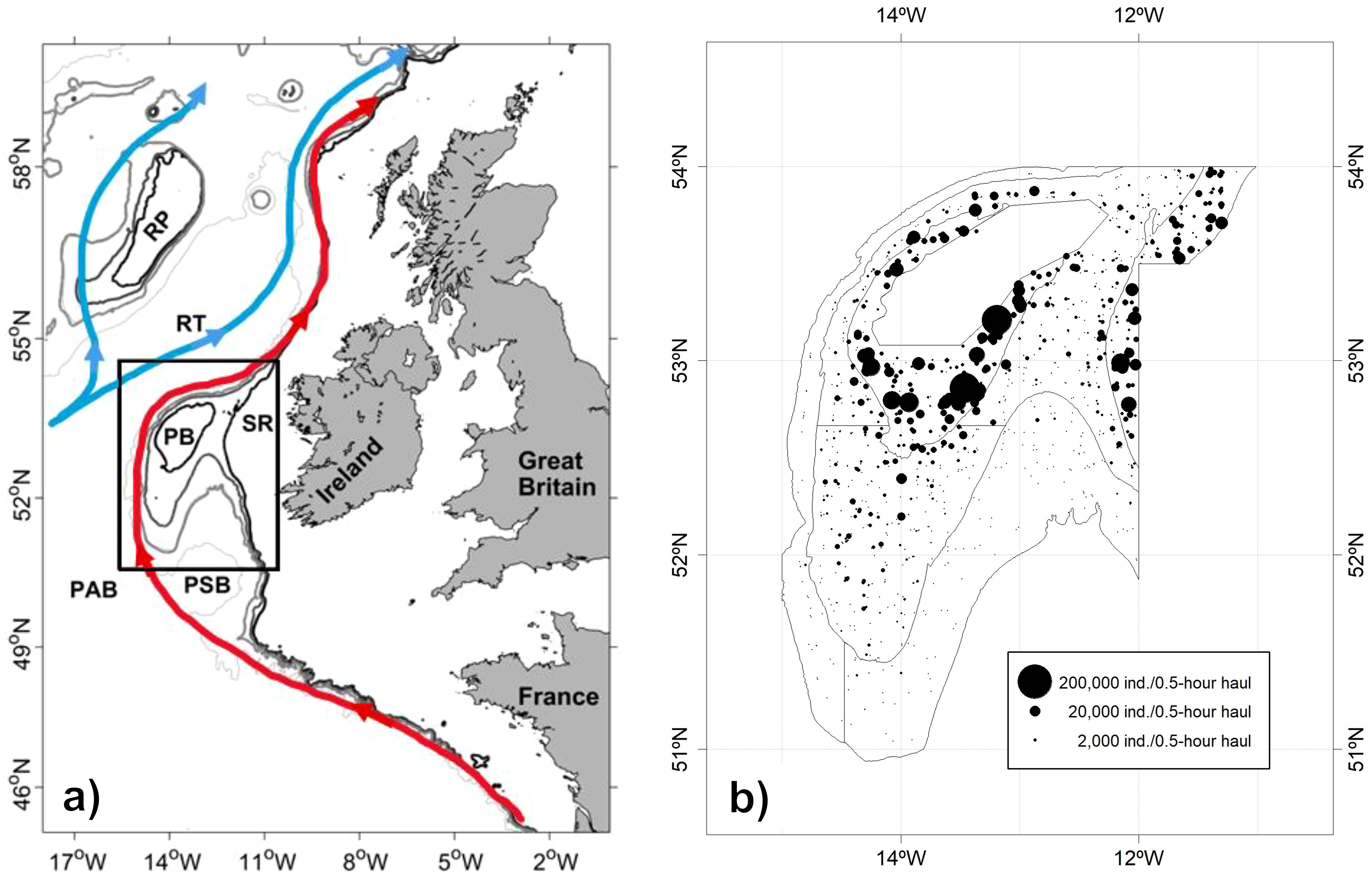
Figure 1. (a) Region of study, showing a schematic of the surface currents pathways (blue: the North Atlantic Current, red: Slope Edge Current). The following isobaths are shown: 300 m (thick black line), 450 m (thick dark grey line), 800 m (thick pale grey line), and 2000 m (thin pale grey line). RP, Rockall Plateau; RT, Rockall Trough; PB, Porcupine Bank; SR, Slyne Ridge; PAB, Porcupine Abyssal Plain; PSB, Porcupine Seabight. The black rectangle shows the sampling region. Adapted from Koman et al. (2022) and Øvrebø et al. (2006). (b) Catch of 0-year class blue whiting (total length < 20 cm) in each haul of the Porcupine survey time series, in number of individuals per 0.5-hour trawl. The boundaries of the Porcupine survey area are highlighted: depth strata are delineated by the isobaths of 300 m (inside the bank), 450 m, and 800 m (outside the bank). The blank area in the center of the Porcupine Bank corresponds to a non-trawlable area.

Spawning mainly occurs from March to May at depths of ~250–600 m (Miesner and Payne, 2018). Blue whiting is known to select optimal oceanographic conditions to maximize the survival of their offspring in the early stages of life, particularly preferring salinities between 35.30 and 35.50. However, spawning locations can vary annually due to fluctuations in the marine environment, which can impact recruitment (Hátún et al., 2009). When the North Atlantic Subpolar Gyre (SPG) is weak, warm (temperature > 9.87°C) and saline (salinity > 35.40) waters from the Eastern North Atlantic Subtropical Gyre enter the spawning area, extending northwards along the European shelf and westwards over the Rockall Plateau (Hátún et al., 2009; Miesner and Payne, 2018). Consequently, spawning occurs at depths with salinities ≥ 35.35 and temperatures ≥ 10°C. These conditions can enhance larval growth and reduce predation, thereby improving survival and recruitment (Hátún et al., 2009; Payne et al., 2012). Conversely, when the SPG is strong, cold (temperature < 9.64°C) and fresh (salinity < 35.38) waters from the North Atlantic restrict high salinities to the Rockall Trough and Porcupine Bank, thereby limiting spawning to these areas (Hátún et al., 2009; Miesner and Payne, 2018). Although variations in blue whiting recruitment may be related to changes in spawning distribution (Miesner and Payne, 2018), they are ultimately driven by the quality of habitat available for early life stages.

Blue whiting eggs are primarily found at depths of 460–580 meters. During the embryonic development, they adjust their neutral buoyancy by adapting to a salinity range from 34 to nearly 40 (Ådlandsvik et al., 2001). Most hatching occurs on the fifth day of incubation (Seaton and Bailey, 1971; Coombs and Hiby, 1979). After hatching, larvae attain neutral buoyancy at a salinity of approximately 36.6, causing them to congregate in the upper 50 m of the water column (Ådlandsvik et al., 2001). The exact duration of the pelagic larval phase is unknown but is estimated to last up to two months (Bailey and Heath, 2001), a crucial period for recruitment dynamics.

One of the main objectives of scientific surveys is to assess recruitment of commercial fish stocks, which is essential for predicting future population sizes and guiding fisheries management. In this study, we present the 2001–2020 record of the Spanish bottom trawl survey, conducted annually in September on the Porcupine Bank. We explore the environmental drivers of blue whiting recruitment, focusing on temperature, salinity, chlorophyll-a (as a proxy for primary productivity), wind mixing index, and relative vorticity during the spawning season (March–May). Besides, we address the effect of the spawning stock biomass from the same year (SSB) and the previous year (SSByear-1) on recruitment. Additionally, we test the hypothesis that the exceptional 0-year-class strength of blue whiting in 2020 resulted from an unusual combination of favorable environmental conditions. By identifying these key environmental factors, we aim to improve our ability to predict future year-class strength and develop more effective fisheries management strategies for blue whiting.

2 Materials and methods

2.1 Study area

The Porcupine Bank (ICES Divisions 7c and 7k) is a large shelf-break bank located approximately 150 to 250 km off the western Irish coast (Figure 1a), covering an area of over 40,700 km². It is a south-north elliptical plateau that forms the north-western margin of the Porcupine Seabight Basin and is characterized by water depths between 300 and 400 m and a width of approximately 100 km (Mohn and White, 2007; Thébaudeau et al., 2016). The slope of the Porcupine Bank on the north and west flanks is steep and narrow towards the Rockall Trough whereas on the south and south-east the bank opens with a gentle slope into the deep embayment of the Porcupine Seabight. At its shallowest point (about 200 km west of Ireland), the Porcupine Bank is typically less than 200 m deep.

In this region, a hydrographic structure known as a Taylor column can develop under low or moderate wind conditions due to the interaction of the local flow with the Porcupine Bank (Kloppmann et al., 2001). In this way, when a steady, homogeneous current encounters the Porcupine bank, it is deflected by the topography and forms a closed anticyclonic circulation around the seamount due to the Earth’s rotation that is known as a Taylor column (White et al., 2007). Under low or no stratification, the Taylor column can reach the ocean surface, but as the stratification increases, it does not extend to the surface and becomes a Taylor cone. This structure is characterized by the doming of isopycnals above the seamount, thus enclosing cold, low-salinity water with an anticyclonic velocity field (Dooley, 1984). The isopycnal doming transports deeper, nutrient-rich water towards the upper layers that might reach the euphotic zone (Genin and Boehlert, 1985). The Taylor column/cone can act as a retention mechanism (Goldner and Chapman, 1997; Mohn et al., 2002) and can induce stratification over the seamount, enhancing productivity (Comeau et al., 1995), though chlorophyll-a levels do not always increase (White et al., 2007).

2.2 Recruitment data

An ongoing Spanish fishery‐independent multi‐species bottom‐trawl survey has been annually conducted on the Porcupine Bank since 2001. One of the main objectives of the survey, carried out in September, is to determine the distribution and relative abundance of recruits of the main commercial species and provide recruitment indices. The survey area extends from 12°W to 15°W longitude and from 51°N to 54°N latitude, following the standard methodology used in the IBTS Northeast Atlantic Surveys (ICES, 2017). The sampling design was randomly stratified into two geographic sectors and three depth strata: < 300 m, 300–450 m, and 450–800 m. Bottom trawls of 30 min at a trawling speed of 3.5 knots were conducted aboard the R/V Vizconde de Eza, a 53 m, 1800 kW stern trawler, using a Baca-GAV 39/52 net with a 20 mm mesh cod end. In each haul, the catch of blue whiting was weighed, and a subsample of 8–10 kg was measured by sex. The stratified mean catch of blue whiting in number of individuals or in terms of biomass per half an hour of trawling was used as the annual index of abundance or biomass. Size-stratified abundance of blue whiting was also estimated by year. Based on otolith age reading (ICES, 2022; 2023), individuals with a total length less than 20 cm were considered 0-year class, i.e., born in the spawning season (March-May) of the same year. Thus, the stratified mean abundance of individuals with a total length less than 20 cm per half an hour of trawling was used as the annual index of recruitment. The survey design and methodology are described in detail in ICES (2017).

As the recruitment data did not meet the assumptions of normality, a one-sample Wilcoxon signed-rank test was applied to evaluate whether annual recruitment significantly differed from the median of the overall time series. Besides, the Holm-Bonferroni correction was applied to take account of multiple comparisons. All statistical analyses were conducted using MATLAB R2023a.

2.3 Remotely sensed and model based environmental data

In order to analyze the potential impact of environmental forcing as drivers of the 0-year class blue whiting recruits, environmental data were obtained from the Marine Copernicus Service (CMEMS) (https://marine.copernicus.eu/) for the period 2001–2020 covering the region of interest (48°-56°N and 16°-8°W). These included maps of monthly means of: (1) satellite-derived Level-4 sea surface temperature (SST, product ID “IFR-L4_GHRSST-SST-ODYSSEA-ATL” for the period 2001–2018 at a spatial resolution of 0.05 degrees, and “IFR-L4-SSTfnd-ODYSSEA-ATL_002” for the period 2019–2020 at a spatial resolution of 0.02 degrees); (2) satellite-derived Level-4 Chlorophyll-a concentration in seawater (product ID “OCEANCOLOUR_ATL_BGC_L4_MY_009_114”, at a spatial resolution of 0.0104 degrees); and (3) 3D fields of temperature, salinity, and ocean currents from the CMEMS Iberian-Biscay-Irish (IBI) Ocean Physics Reanalysis monthly products (“CMEMS IBI-MFC” for the period 2001-2018, at a spatial resolution of 0.0833 degrees, and “IBI-MFC (PdE Production Center)” for the period 2019-2020, at a spatial resolution of 0.0278 degrees). The IBI products are provided at 50 vertical levels using a z-type grid that ranges from a surface level at 0.5 m to the deepest level at 5698 m. Therefore, the products’ vertical resolution varies from ~1.05 m at the surface to ~453.13 m at the deepest level. The full time series (2001-2020) was created by spatially interpolating the 2001–2018 fields to the same spatial resolution as the 2019–2020 fields. The ocean currents were used to calculate the relative vorticity as the curl of the horizontal velocity vector. Finally, monthly means of the ERA5 wind field at 10 m were retrieved from the Copernicus Climate Data Store (https://cds.climate.copernicus.eu/) with a spatial resolution of 0.25 degrees. A wind mixing index (WMI) was calculated as the cube of wind speed, following Cuttitta et al. (2006).

All data were subsampled to retain only the main spawning months (i.e., March, April, and May). The 3D fields (temperature, salinity, currents, relative vorticity) were vertically averaged over the blue whiting spawning depth to provide a proxy for the environmental conditions experienced by the blue whiting eggs at the time of spawning. The depth range (250–600 m) was selected as in Miesner and Payne (2018) and Miesner et al. (2022). Data were averaged across the region of interest and, whenever the bathymetry was shallower than 250 m, the data closest to the seafloor were used. A Wilcoxon Signed-Rank Test was separately performed for each spawning month to test the null-hypothesis that the depth-averaged values of each year were significantly different from the median of the corresponding month time series.

In addition, to assess whether a Taylor column/cone could develop over the Porcupine Bank, three non-dimensional numbers were calculated, namely, the Rossby number, Ro = U/(f×L), the relative height of the seamount to the water depth, α = h₀/H, and the blocking parameter, Bl = α/Ro (White et al., 2007; Ma et al., 2021), where U (m/s) is the ambient current velocity, f (rad s⁻¹) is the Coriolis parameter, L (m) is the width of the Porcupine Bank, h₀ (m) is its height and H (m) is the water depth. The threshold values for the formation of a Taylor column may slightly change under different conditions but in general, a Taylor column cannot be generated if Ro > 0.15-0.2 (Chapman and Haidvogel, 1992) or if Bl < 1-2 (Hogg, 1973; Owens and Hogg, 1980; Chapman and Haidvogel, 1992; Martin and Drucker, 1997). Finally, the 3D currents, relative vorticity, temperature, and salinity fields were analyzed over the Porcupine Bank to confirm the existence of a Taylor column. More specifically, the currents velocity and relative vorticity fields were used to verify the existence of an anticyclonic circulation field over the Porcupine Bank. Additionally, 3D profiles of temperature and salinity were extracted along a longitudinal section placed at 53°N to explore whether the isopycnals were doming above the bank enclosing cold and low-salinity water over it.

All the data extraction and analyses (one-sample Wilcoxon signed-rank test and Holm-Bonferroni correction) were performed using the MATLAB R2023a software package.

2.4 Lagrangian simulations

In order to assess the importance of advection and retention processes on recruitment, a Lagrangian study was undertaken using Opendrift (Dagestad et al., 2018) as the development platform. The Lagrangian model was coupled to the CMEMS IBI – Ocean Physics Reanalysis daily fields as physical forcing. The numerical core of the IBI model is based on the NEMO v3.6 ocean general circulation model, run with a horizontal resolution of 1/12°. Altimeter data, in-situ vertical profiles of temperature and salinity, and satellite sea surface temperature are assimilated.

A Lagrangian simulation was carried out for each year from 2001 to 2020. For each simulation, 10,000 particles were released at 300 m depth at position 53.5°N, 14°W and were temporally distributed using a normal distribution centered on 15 March (Bailey, 1982; Hillgruber and Kloppmann, 1999, 2000). The particle dispersion model incorporated two development phases: the first phase represented the pelagic egg state, with an average duration of 5 days (Seaton and Bailey, 1971; Coombs and Hiby, 1979), and the second one corresponded to the larval stage, which was assumed to last up to two months (Bailey and Heath, 2001). The larvae were assigned behavior that directed them to a depth of 50 m, based on current knowledge of this process (Ådlandsvik et al., 2001). More specifically, if larvae are displaced from a depth of 50 m due to physical processes, they swim upwards or downwards until they reach that depth. The Runge-Kutta advection scheme was used, and vertical advection was estimated using the Sundby (1983) approximation, which derives eddy diffusivity from wind speed. Two-month simulations were run for each year with this configuration to cover the early stages of larval development where environmental variability plays the most important role in larval success (Bailey and Heath, 2001).

Using the trajectory results, a retention index (N50) was calculated as the percentage of particles that traveled less than 50 miles. A one-sample Wilcoxon signed-rank test was performed followed by the Holm-Bonferroni correction (MATLAB R2023a software package) to determine whether the N50 for each year was significantly (at the 95% confidence level) higher or lower than the median.

2.5 Quantile regression

Quantile regression (Mosteller and Tukey, 1977; Koenker and Bassett, 1978) is a statistical technique widely used in quantitative modelling. It allows a regression curve to be fitted to a different part of the statistical distribution of the response variable. Mosteller and Tukey (1977) realized that it was possible to fit regression curves to parts of the distribution of a response variable other than the mean. Although this was possible, it was rarely done and consequently many of the regression analyses gave an incomplete picture of the relationship between the variables. In ecology, a regression model with heterogeneous variances implies that there is no single rate of change that characterizes changes in the probability distribution of the response variable (Cade and Noon, 2003). Focusing only on changes of the mean may underestimate, overestimate, or simply fail to distinguish truly non-zero differences in heterogeneous distributions (Cade et al., 1999).

Quantile regression was used in this study (MATLAB R2023a software package) to explore the relationships between the 95% quantile of blue whiting recruitment and a set of candidate explanatory variables. These included environmental variables (i.e., temperature, salinity, WMI, relative vorticity, and chlorophyll-a), the N50 retention index, and the spawning stock biomass (SSB and SSByear-1). Temperature and salinity were included due to their direct influence on the physiological processes of blue whiting, particularly during spawning and larval development. Chlorophyll-a was used as an indicator of primary productivity and potential food availability for larvae and juveniles. Meanwhile, WMI and relative vorticity were considered due to their roles in nutrient dynamics and plankton distribution. The N50 retention index was used to evaluate the impact of advection and retention processes on recruitment. Spawning stock biomass was introduced to investigate stock–recruitment relationships, whether from the same year or the previous year, as it represents the reproductive potential of the population.

Quantile regression was used to investigate how environmental and biological factors are associated with high levels of blue whiting recruitment, focusing on the upper tail of the recruitment distribution (e.g., the 95th percentile). The analysis was motivated by the exceptionally high recruitment observed in 2020, which served as a reference point to explore potential drivers of extreme recruitment events. By examining high quantiles (> 90th), the model provides insight into the maximum expected recruitment for a given value of a forcing factor (e.g., chlorophyll-a as a proxy for food availability), under the assumption that other modulating factors are not limiting. For this purpose, a spatially-averaged time series was extracted for each depth-averaged environmental variable (see section 2.3) by averaging them over the region enclosed within the shallowest stratum (< 300 m), which included the Porcupine Bank and the region over the adjacent continental shelf, between the 200 m and 300 m bathymetric lines. Finally, a quantile regression was performed for recruitment using the monthly means of each (spatially and depth-averaged) environmental variable for March, April, and May, respectively, the N50 retention index obtained from the Lagrangian simulations, and the SSB and SSByear-1 from the ICES (2022) report. Finally, the Holm-Bonferroni correction was applied to take account of multiple comparisons.

Additionally, to evaluate the interactions between the variables influencing recruitment, a multiple quantile regression model was performed using the Python statistical package statsmodels. A step-forward process was followed, with variables being added based on the lowest p-value as the entry criterion.

3 Results

3.1 Recruitment

Figure 2 shows the stratified indices of blue whiting biomass and recruitment over the 20-year time series of the Porcupine Survey. The Wilcoxon signed-rank test indicated that those years with recruitment values significantly higher than the median (at the 95% confidence level) were 2003, 2004, 2007, 2009, 2010, 2015, and 2020. In 2020, the stratified mean abundance reached 7321 ± 2618.7 recruits per haul, the highest recorded to date, representing 1.6 and 2.1 times the recruitment levels seen during the peaks of 2003 and 2004, respectively. Additionally, 2020 not only recorded the highest stratified mean abundance of recruits, but also the highest stratified mean biomass of blue whiting. The recruitment peak in 2020 is further evident in Figure 3, which shows the size-stratified abundance by year. On the other hand, recruitment was significantly lower than the median in 2005, 2011, 2012, 2013, 2014, 2017, and 2019, with 2014 presenting the lowest value of the time series with 306 ± 75.7 recruits per haul.

Figure 2

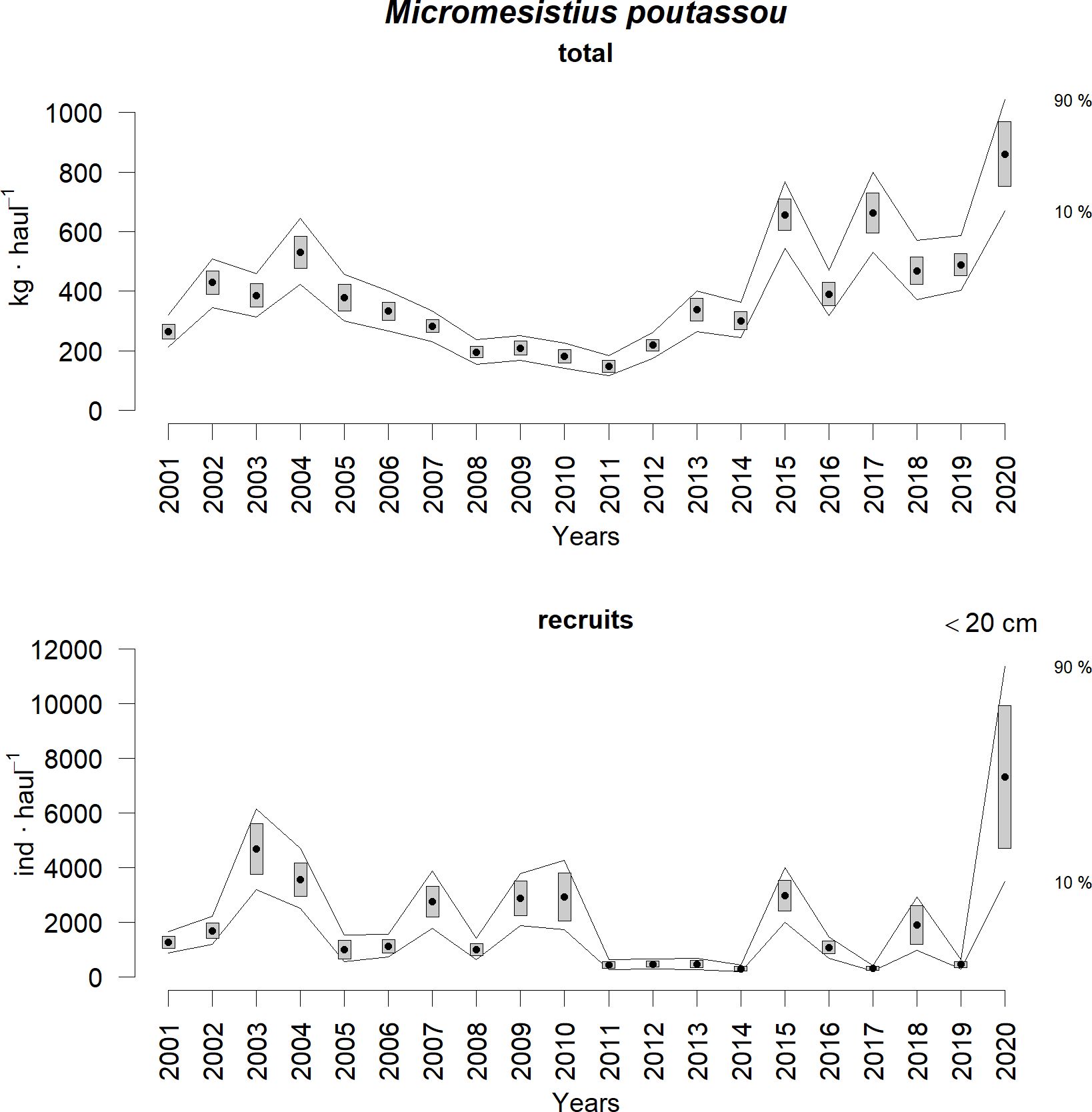
Figure 2. Stratified blue whiting biomass index (top panel) and stratified blue whiting 0-year class abundance index (bottom panel) in the Porcupine Survey time series (2001-2020). Boxes mark the parametric standard error of the stratified abundance indices; lines mark the bootstrap confidence intervals (α = 0.80, bootstrap iterations = 1000).

Figure 3

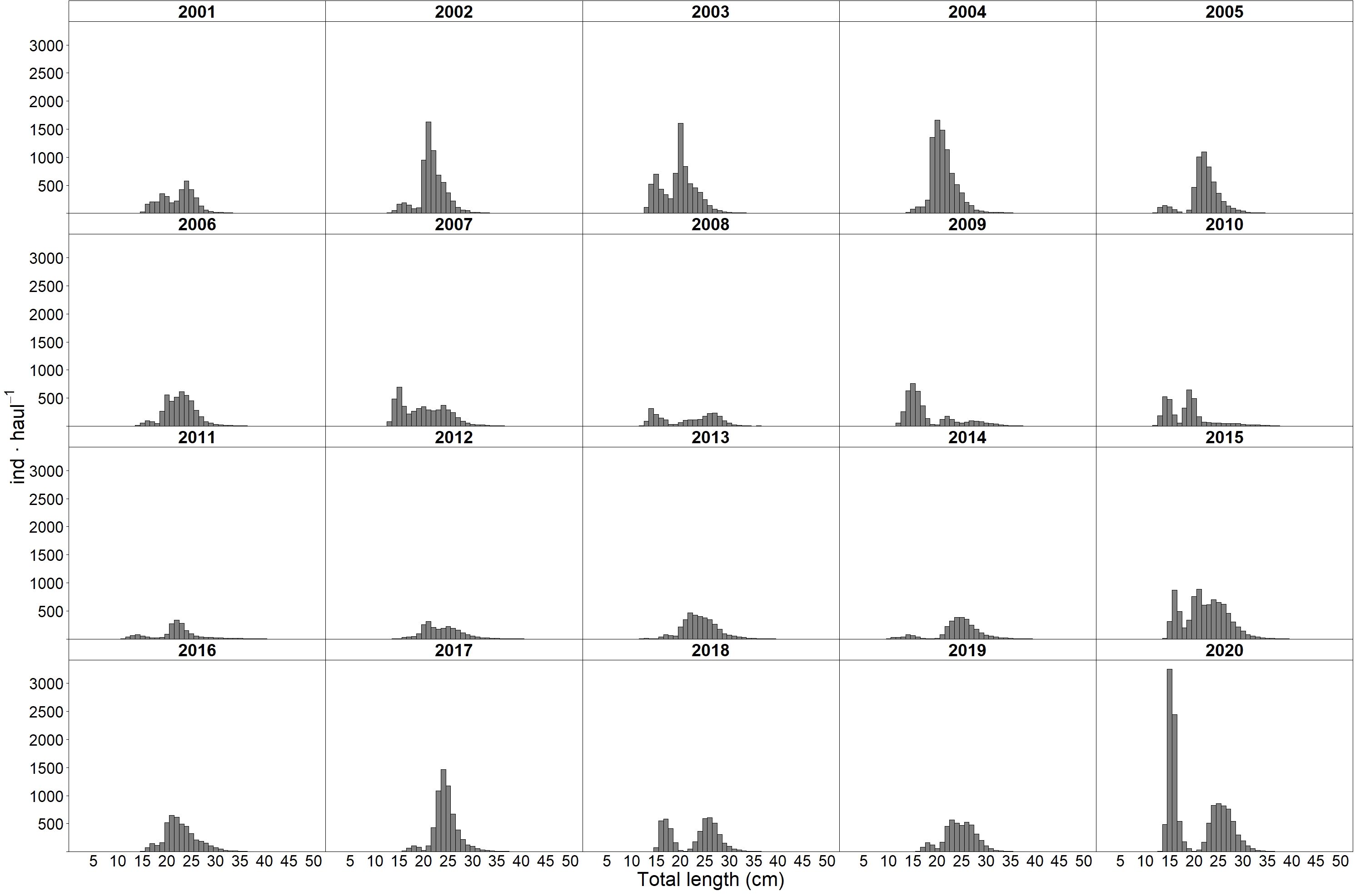
Figure 3. Length distribution of blue whiting in the Porcupine survey time series.

As observed in Figure 1b, recruits were primarily concentrated in the shallower stratum (< 300 m), comprising the central area of the bank and the Slyne Ridge, which connects the bank to the continental shelf. In fact, more than 70% of the recruits were captured within this depth range across the time series.

3.2 Environmental conditions

The depth-averaged (250–600 m) temperature (Supplementary Figures S1–S3) and salinity (Supplementary Figures S4–S6) anomaly maps showed warmer and more saline conditions between 2002-2012, with a notable inter- and intra-annual variability. Monthly wind averages also showed a significant inter-annual variability during the spawning season (March to May), both in terms of wind speed and direction, with the highest intensities in March and the lowest ones in April. In particular, wind speeds were exceptionally low (< 0.9 m s⁻¹) over the Porcupine Bank in April 2020. Furthermore, while in previous years winds typically blew from the west (W, NW or SW), in April 2020 they blew from the east. This variability is also evident in the WMI anomalies (Figure 4; Supplementary Figures S7, S8), with both inter- and intra-annual variability.

Figure 4

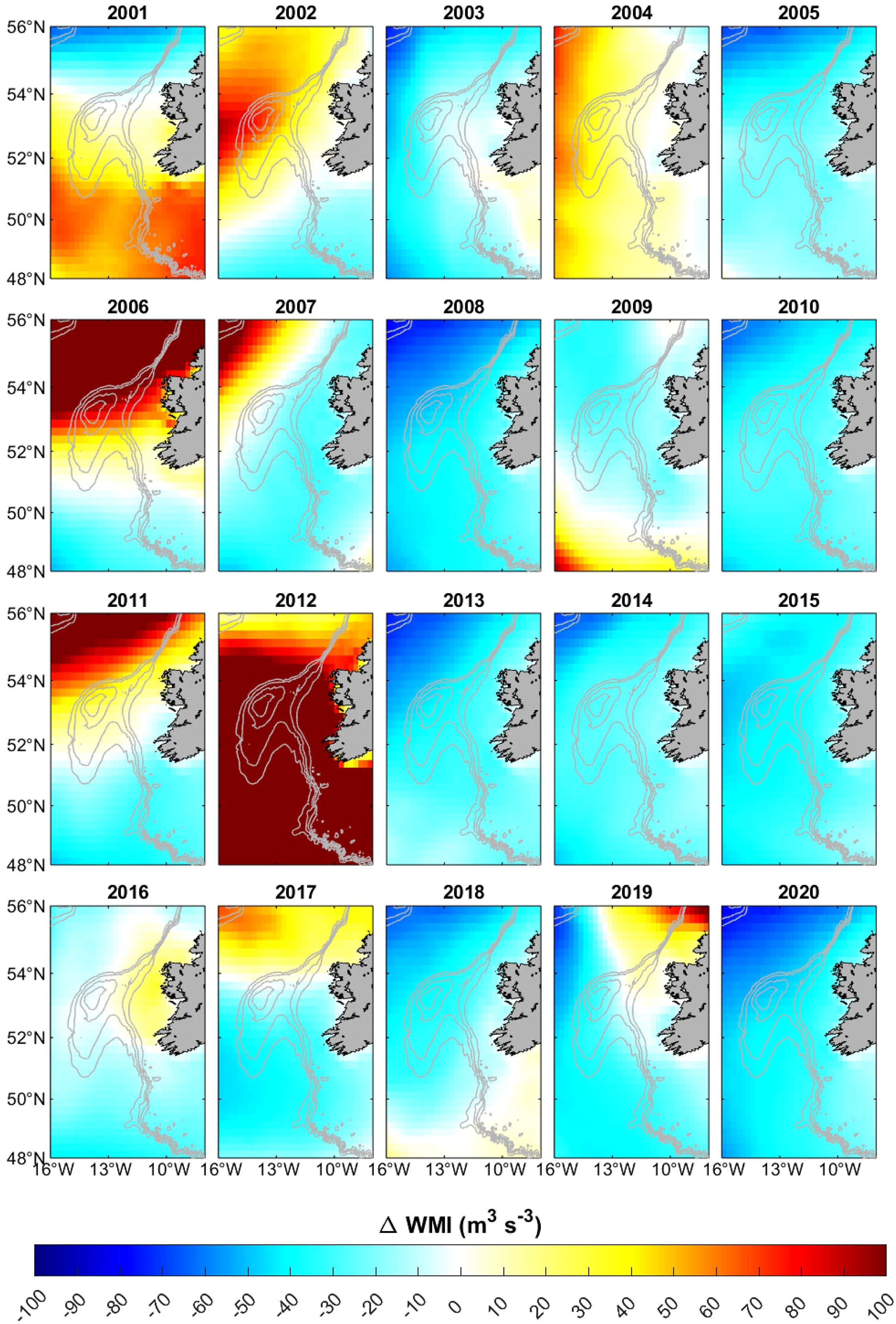
Figure 4. Wind mixing index (WMI) anomalies for April between 2001 and 2020. The 200, 300, 500, and 1000 m isobaths are shown (thick grey line). Years where WMI is significantly different from the median are 2002, 2004, 2005, 2006, 2008, 2010, 2011, 2012, 2013, 2015, 2018, and 2020.

The IBI model showed weak monthly depth-averaged (250–600 m) currents on the Porcupine Bank throughout the spawning period, ranging between 2–7 cm s⁻¹ and 1–5 cm s⁻¹ for March and April, respectively. However, while their direction was either northward or north-westward between 2001 and 2018, in 2019 and 2020 they formed an anticyclonic gyre over the shallowest stratum of the Porcupine Bank, with more intense currents on the western side of the bank. In March and April 2020, the 3D velocity field was almost barotropic, with a column-like vertical structure occupying the entire water column (Figure 5), suggesting the existence of a persistent Taylor column circulation above the bank. This structure was also observed in May 2020, but only down to 40–50 m depth, indicating instead the presence of a Taylor cone. A very similar situation was observed in spring 2019.

Figure 5

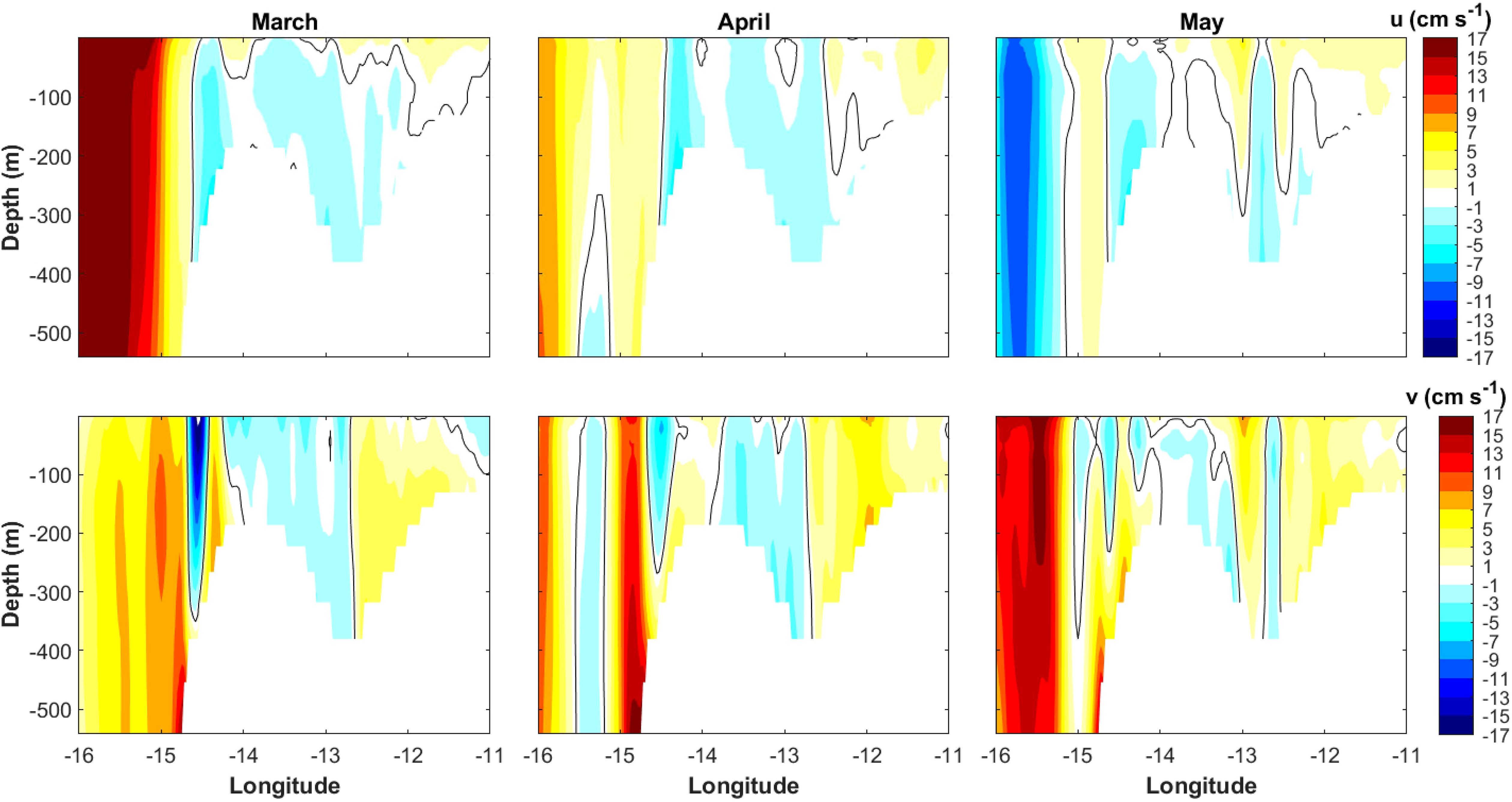
Figure 5. Monthly means of zonal (u, top panel) and meridional (v, bottom panel) currents profiles during the 2020 blue whiting spawning period of March, April, and May along the 53°N line. The black line delimits the zero-value.

This anticyclonic circulation was confirmed by the negative depth-averaged relative vorticity, which showed values of ~ −0.1 s⁻¹, −0.2 s⁻¹, and −0.06 s⁻¹ in March, April, and May 2020, respectively. During previous years, however, the depth-averaged relative vorticity presented absolute values between one and two orders of magnitude lower (positive or negative, depending on the year) (see the depth-averaged relative vorticity anomaly maps in Supplementary Figures S9–S11). Evidence of a closed anticyclonic circulation was also found in 2019, when the vertical currents structure and the temperature and salinity profiles suggested the existence of a Taylor column in April and a Taylor cone in March and May. The presence of a persistent Taylor column or cone during the 2020 spawning season is also supported by the IBI model temperature and salinity profiles (Figure 6), in which a doming of cool (temperature ~9.5-9.7°C) and fresher (salinity ~35.37-35.40) waters can be observed above the Porcupine Bank from March to May, reaching the surface in March and April. Furthermore, a core of lower temperature over the Porcupine Bank was also observed on the satellite SST monthly maps in March and April 2020 (Supplementary Figures S12, S13), confirming the existence of a Taylor column that reached the surface. As for the rest of the years, while an uplift of the isotherms is generally observed on the Porcupine Bank, the isohalines are only uplifted during the years identified as cold and fresh. However, in all cases the conditions for the generation of a Taylor column/cone were met, i.e., Ro << 0.15, and Bl >> 2, indicating that the environmental conditions were sufficient for the development of a Taylor column.

Figure 6

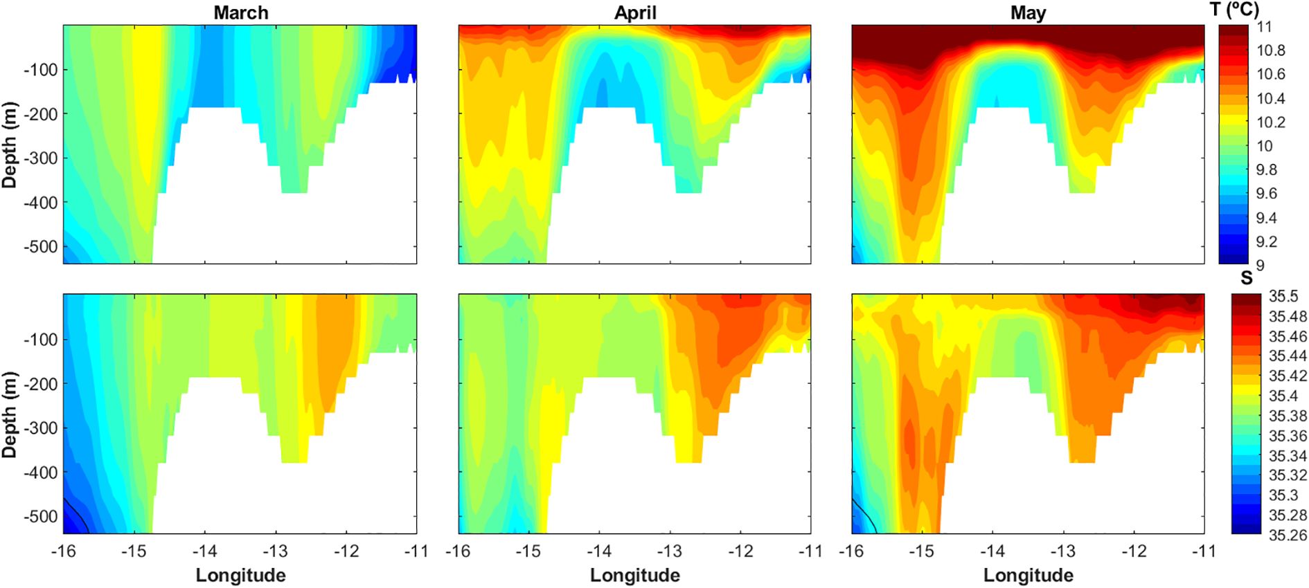
Figure 6. Monthly means of temperature (T, top panel) and salinity (S, bottom panel) profiles during the 2020 blue whiting spawning period of March, April, and May along the 53°N line.

Chlorophyll-a concentrations were low in March throughout the time series (mean values ~0.19 mg m⁻³ over the shallowest stratum), although they showed a notable inter-annual variability (Supplementary Figure S14). In contrast, the chlorophyll-a concentrations increased in April exhibiting a pronounced spatial and inter-annual variability (Figure 7). For example, in years like 2008, 2013, and 2016, negative anomalies were observed across the entire region, corresponding to chlorophyll-a concentrations that were significantly lower than the median. Other years, such as 2003, 2014 or more notably 2020, presented significantly larger concentrations. Finally, it is worth noting the high chlorophyll-a values observed in May 2004 (Supplementary Figure S15).

Figure 7

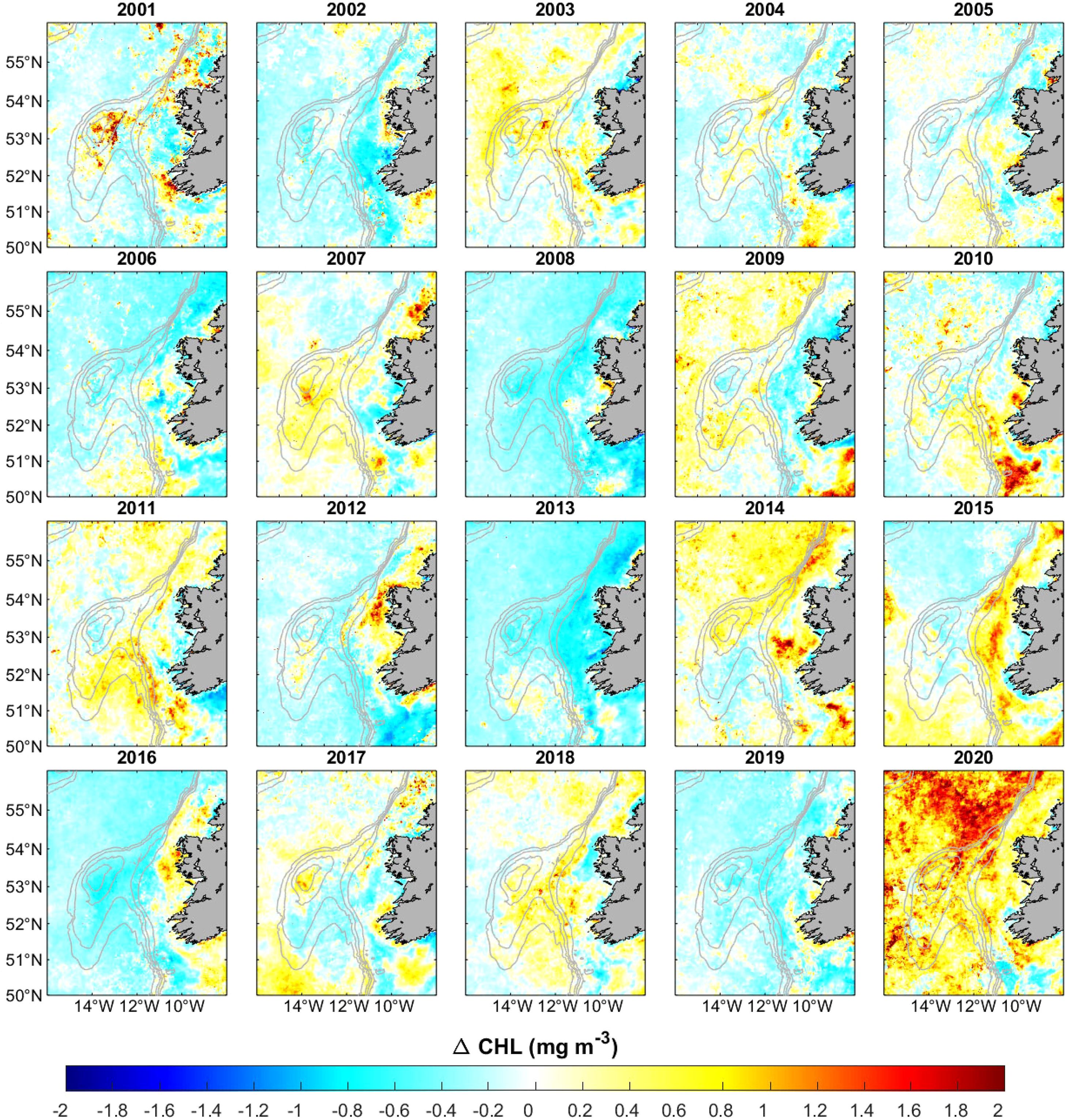
Figure 7. Satellite chlorophyll-a (CHL) anomalies for April between 2001 and 2020. The 200, 300, 500, and 1000 m isobaths are shown (thick grey line). Years where CHL is significantly different from the median are 2001-2003, 2006-2008, 2013, 2014, and 2016-2020.

3.3 Lagrangian simulations

The Lagrangian simulations showed different dispersion scenarios during the study period (Supplementary Figure S16), ranging from years with little advective activity to years with significant particle displacement, as evidenced by the N50 retention index (Figure 8a). In particular, the Wilcoxon signed-rank test indicated that significantly high particle dispersion was observed in 2002, 2004, 2008, 2013, 2015, 2017, and 2018 (Figure 8b), based on this index. In contrast, years such as 2003, 2005, 2011, 2014, 2016, and 2020 showed significantly high retention indexes. Among these, 2003 and 2020 stand out, since the highest number of particles remained in the vicinity of the Porcupine Bank (Figure 8a), traveling only short distances from the release location (Supplementary Figure S16; Figure 8c).

Figure 8

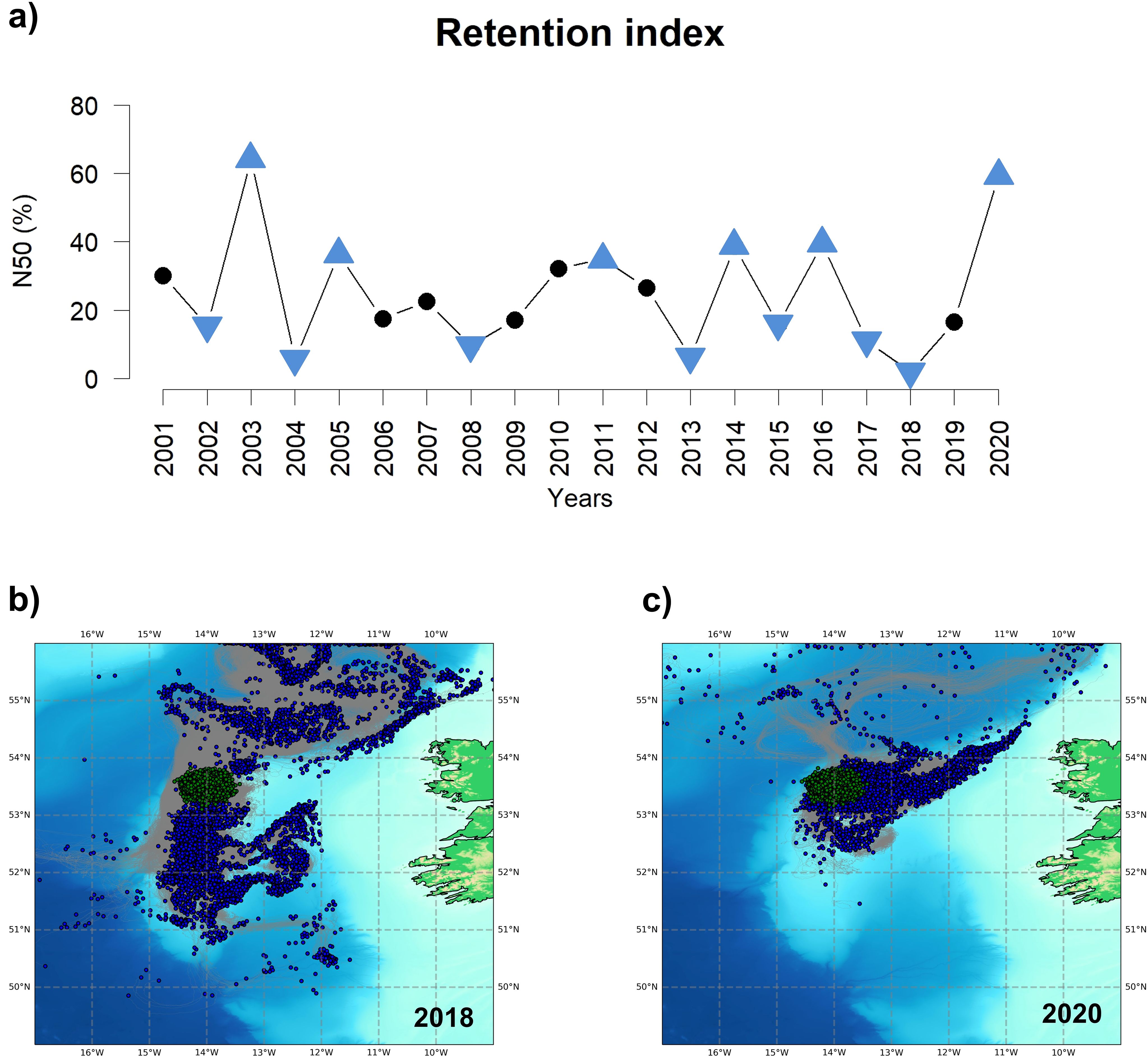
Figure 8. (a) Time series of the N50 retention index expressed as the percentage of particles that moved less than 50 nautical miles. Blue triangles mark those years with a N50 value significantly different from the median at the 95% confidence interval. (b) 2018 and (c) 2020 Lagrangian simulations showing the particles’ initial position (yellow dots), trajectory (grey lines), and final position (blue dots).

3.4 Quantile regression

The quantile regression fit applied on blue whiting recruitment only showed significant relationships with the explanatory variables chlorophyll-a and WMI in April, as well as with N50 (Table 1). The relationship between recruitment and chlorophyll-a concentration and between recruitment and N50 were positive, while the relationship with WMI was negative. In contrast, the quantile regressions for SSB and SSByear-1 showed no significant relationship with recruitment or any of the environmental variables.

Table 1

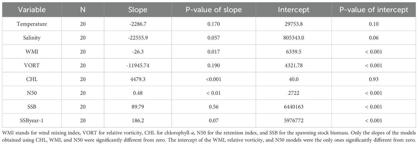
Table 1. Results of the quantile regression fitted on the quantile 0.95 of the blue whiting recruitment.

A multiple quantile regression model was calculated to evaluate the overall response of recruitment to the variables considered in this study (i.e., temperature, salinity, WMI, relative vorticity, chlorophyll-a, the N50 retention index, SSB, and SSByear-1). Prior to this, a cross-correlation matrix was calculated to rule out variables exhibiting strong collinearity. No significant correlations were found among the variables. Multicollinearity was further evaluated using the variance inflation coefficient, which consistently yielded values close to 1, reflecting no significant multicollinearity issues. The resulting model was:

$$Recruitment=4730*CHL-1.7*WMI(n=20,Pseudo{R}^2=0.64)$$

Both variables presented p-values lower than 0.001 and the y-intercept not significantly different from zero.

4 Discussion

The recruitment process in blue whiting (Micromesistius poutassou) is highly complex, shaped by multiple interacting factors that make it difficult to disentangle their relative importance. In this study, the abundance of 0-year-class blue whiting recruits (total length < 20 cm) recorded during the Spanish bottom trawl survey on the Porcupine Bank (in September, from 2001 to 2020) was analyzed. Recruitment patterns were examined in relation to several environmental variables derived from remotely sensed and model data for the spawning season (March-May) as well as with results from Lagragian transport simulations and SSB and SSByear-1 data from the ICES (2022) report. Our findings reveal substantial interannual variability in both meteorological and oceanographic conditions over the study area, as well as in blue whiting recruitment.

Previous studies suggested that when the North Atlantic Subpolar Gyre is weak, resulting in warmer and more saline conditions, blue whiting spawning extends to the Rockall Plateau, potentially enhancing recruitment due to factors such as increased phytoplankton and warm-water zooplankton abundance or reduced predation by mackerel (Hátún et al., 2009; Payne et al., 2012). Despite the period from 2002 to 2012 being classified as warm and saline (Miesner and Payne, 2018), our study showed significantly strong recruitment only in certain years (2003, 2004, 2007, 2009, and 2010; Figure 2), while others showed significantly low recruitment values (i.e., 2005, 2011, 2012). This suggests that recruitment variability is driven by factors beyond large-scale environmental conditions.

The Wind Mixing Index (WMI) also played a role, with April values during this warm and saline period significantly lower than the median only in 2005, and significantly higher in 2004, 2011, and 2012. The low recruitment values in 2011 and 2012 may be linked to turbulence-induced larval malnutrition, which is often associated with high WMI (Hillgruber and Kloppmann, 1999; 2000). However, these WMI variations did not always align with recruitment levels, since 2004 was characterized by high recruitment values under high WMI in April while 2005 showed low recruitment values and low WMI, highlighting the complexity of recruitment dynamics. Nevertheless, quantile regression revealed a significant negative relationship between WMI and recruitment, indicating that, in general, lower WMI values during April tend to favor recruitment, likely by enhancing prey availability and larval survival.

Similarly, chlorophyll-a concentrations, as a proxy for phytoplankton biomass, did not consistently correlate with recruitment during warm and saline years. For instance, while high chlorophyll-a concentrations in April 2003 and 2007 could partially explain strong recruitment, other years with strong (2004, 2009) or weak (2005, 2011, 2012) recruitment exhibited chlorophyll-a concentrations that were not significantly different from the median. Interestingly, in 2004, despite the low chlorophyll-a values during March and April, exceptionally high chlorophyll-a levels were recorded in May (~ 0.8–2 mg m⁻³, Supplementary Figure S15), which, in conjunction with low WMI (Supplementary Figure S8), may indicate a delayed spawning season. This suggests that other factors, such as timing and spatial distribution of primary production, may influence recruitment. In any case, the quantile regression showed a positive and significant relationship between the chlorophyll-a in April and recruitment, supporting the relevance of food availability during early larval stages.

In contrast to warm and saline years, blue whiting spawning is generally restricted to the European Continental Shelf and the Porcupine Bank during cooler and fresher (i.e., with lower salinity) years, conditions typically associated with lower recruitment (Hátún et al., 2009). However, our study found that 2020, a cold and fresh year, produced the strongest recruitment in the 2001–2020 record of the Spanish bottom trawl survey on the Porcupine Bank (Figure 2). The environmental conditions that year were exceptionally favorable, featuring the highest chlorophyll-a values in the time series, the second-highest N50 retention index, and the second-lowest WMI, factors likely contributing to the remarkable recruitment observed. This again highlights the complex and non-linear relationship between recruitment and its drivers. Additionally, the temperature and salinity range values (temperature ~9.5-9.7°C, salinity ~35.37-35.40) during the March and April 2020 profiles (Figure 6) seemed optimum for blue whiting spawning (Miesner and Payne, 2018), which may have provided favorable water density conditions for their eggs and larvae within the entire spawning depth. Nevertheless, further analysis with higher temporal and spatial resolution data would be needed to draw conclusions concerning the influence of water density.

The strong recruitment in 2020 suggests that, while larval observation is typically less frequent during cold and fresh years (Miesner and Payne, 2018), specific environmental conditions may still favor recruitment. For instance, low WMI can enhance larval survival by increasing prey availability due to reduced wind-driven turbulence, thereby improving feeding success (Kloppmann et al., 2002). In our study, quantile regression confirmed a significant negative relationship between WMI and recruitment, supporting the role of this mechanism. This aligns with the significant positive relationship observed between the N50 retention index and recruitment, indicating that larval retention and stability in the recruitment zone are critical factors.

Moreover, sustained low or moderate wind conditions could trigger the onset of a persistent Taylor column circulation over the Porcupine Bank, acting as a retention mechanism of blue whiting larvae (Kloppmann et al., 2001). In this study, in spite of the low WMI observed throughout the spawning season in 2005, 2010, 2016, 2017, 2018, and 2020, a closed anticyclonic circulation indicative of the presence of a Taylor column was only detected in 2020. The moderate wind conditions in March 2020, and particularly the notably calm conditions in April 2020, promoted the generation of a persistent Taylor column/cone circulation over the Porcupine Bank, as evidenced by the doming of cool and low-salinity waters. The doming of isopycnals in this region is a typical feature under low to moderate wind conditions, as previously reported with in situ data (e.g., Ellet and Turrell, 1992; Titov et al., 1993; McMahon et al., 1995; Kloppmann et al., 2001). Furthermore, the negative relative vorticity indicated a closed anticyclonic circulation within the entire water column (March-April) or most of it (May), thus confirming the existence of the Taylor column (March-April) or cone (May) during the 2020 spawning season (March to May). Therefore, the strong recruitment in 2020 suggests that larval retention and food availability played a crucial role. Although this structure is common in the region, it can be eroded by strong vertical mixing caused by storm-induced high current speeds (Kloppmann et al., 2001; Mohn et al., 2002). Under such conditions, currents flowing towards the bank typically generate a meander around it, rather that forming the closed anticyclonic circulation characteristic of a Taylor column (Kudlo et al., 1984). Since the data used in this study correspond to monthly means, it may be assumed that the moderate (March 2020) or low (April 2020) wind conditions, and hence the Taylor column circulation, prevailed above the Porcupine Bank during both months, acting as a retention mechanism, as also suggested by the Lagrangian simulations. Although this structure was also suggested by the vertical currents and the temperature and salinity profiles between March and May 2019, the relatively low retention index obtained in the Lagrangian simulations indicated otherwise. Moreover, the sporadic generation of a short-lived Taylor column circulation in other years cannot be ruled out, as it may not be visible in the monthly mean data used in this study.

The observed isopycnal doming can transport nutrient-rich water to the upper layers, promoting primary production (Genin and Boehlert, 1985). As mentioned above, the highest chlorophyll-a concentrations in the region were observed in April 2020, with average values between 1.2–1.6 mg m⁻³ over the Porcupine Bank. Since chlorophyll-a is a proxy of phytoplankton biomass, and its concentrations above 0.2 mg m⁻³ indicate sufficient planktonic life to sustain fisheries (Butler, 1988), it is expected that the secondary productivity was particularly enhanced during that month, providing sufficient food for blue whiting larvae. This was confirmed by the quantile regression, which showed a strong, positive, and significant correlation between the chlorophyll-a concentration and recruitment. Therefore, our results suggest that the Taylor column/cone observed during the 2020 blue whiting spawning months supports the retention/enrichment/concentration hypothesis proposed by Bakun (2010), wherein successful recruitment is conditioned by the co-occurrence of: i) an enrichment mechanism that increases primary and secondary productivity and food availability for larvae; ii) a retention mechanism that prevents egg and larval loss from the spawning/nursery area; and iii) a concentration mechanism that aggregates food and larvae to enhance trophic interactions.

Consequently, our results suggest that eggs and larvae need to remain close to the bank, but they also require sufficient primary production to support above-average recruitment. This was evident in 2003 and 2020, when both retention and primary production aligned, leading to significantly higher larval viability compared to other years. Conversely, even if particles are advected away from the bank, strong recruitment can still occur during exceptional primary production events, such as in 2004, which showed a low N50 retention index but the highest chlorophyll-a anomalies of the time series in May. Therefore, when both advection and primary production are at intermediate levels, recruitment will likely fall within the mid-range. However, if either factor creates a scenario favorable for increased recruitment, and the other does not counteract, above-normal recruitment levels can be achieved. In fact, the quantile regression indicated that high phytoplankton concentrations, low WMI and high N50 retention index are necessary conditions to obtain high recruitment values. Other variables, such as the spatially- and depth-averaged temperature and salinity or the SSB and SSByear-1 showed no significant correlations with recruitment (p-value > 0.05). Although quantile regression does not offer precise recruitment predictions due to the nature of the monthly-average data, it serves as a valuable tool for resource management in specific scenarios. In this case, it provides crucial insight into the potential maximum recruitment based on a forcing variable, helping to assess whether the coming year is likely to be a good or poor recruitment year for the species. The information derived from this statistical method, using the 0.95 quantile, indicates the maximum expected value of the response variable (recruitment) given an explanatory variable (i.e., phytoplankton) in a scenario where other drivers are favorable.

This study demonstrates that the environmental conditions during the 2020 blue whiting spawning season, particularly in April, were exceptionally favorable for larvae survival over the Porcupine Bank, leading to a unique recruitment event within the 20-year time series. Despite of the local focus of the Spanish bottom trawl research survey, our findings align with the high recruitment estimated for 2021 (71.6 billion) and the record survey index for age-2 in 2022, both corresponding to the 2020 year-class, as reported by ICES (2022). In this context, the 2022 assessment showed a strong increase in the SSB and an 81% increase in catch recommendations for 2023, compared to 2022. Therefore, the results of this study enhance our understanding and management of the recruitment process for this species.

5 Conclusions

The analysis of 0-year class blue whiting recruits from the 2001–2020 records of the Spanish bottom trawl survey on the Porcupine Bank (September) in relation with environmental variables during the spawning season (March-May) revealed key insights into the drivers of recruitment success. While the entire time series was examined, particular attention was given to 2020, which recorded the highest recruitment levels in the 20-year period, being 1.6 and 2.1 times higher than the peaks observed in 2003 and 2004, respectively.

Results highlighted the complexity of blue whiting recruitment, which does not always respond predictably to similar environmental conditions. Key conclusions include:

● Wind mixing index (WMI), chlorophyll-a and the N50 retention index were identified as the main environmental variables affecting recruitment.

● Low WMI was associated with high recruitment, suggesting that reduced wind-induced turbulence improves larval survival by enhancing feeding conditions.

● Sustained low wind conditions may trigger the onset of a Taylor column, which can act as a retention mechanism for larvae and their prey, therefore fostering larval survival.

● The Taylor column may also uplift nutrient-rich waters into the euphotic zone, promoting high chlorophyll-a concentrations.

● Chlorophyll-a concentrations correlated positively with recruitment, reinforcing the importance of primary production for larval success.

● Above-average recruitment is triggered by the conjunction of low wind-induced turbulence, high larval retention, and enhanced primary production, even under low spawning stock biomass.

Data availability statement

The raw data supporting the conclusions of this article will be made available by the authors, without undue reservation.

Author contributions

IL: Conceptualization, Data curation, Formal analysis, Methodology, Software, Validation, Visualization, Writing – original draft, Writing – review & editing, Funding acquisition. MC: Formal analysis, Methodology, Software, Validation, Visualization, Writing – original draft, Writing – review & editing. GG-N: Formal analysis, Methodology, Software, Validation, Visualization, Writing – review & editing. FV: Software, Supervision, Writing – review & editing. FB: Conceptualization, Data curation, Investigation, Methodology, Supervision, Visualization, Writing – original draft, Writing – review & editing, Funding acquisition.

Funding

The author(s) declare financial support was received for the research and/or publication of this article. The survey, included in the PORCUDEM project (PORCUDEM-20233FMP001), was partly funded by the EU through the European Maritime, Fisheries and Aquaculture Fund (EMFAF) within the Spanish National Program of collection, management, and use of data in the fisheries sector and support for scientific advice regarding the Common Fisheries Policy. Masuma Chowdhury was partly supported by a grant funded by the European Commission under the Erasmus Mundus Joint Master Degree Program in Water and Coastal Management in the 2018/2019 class (WACOMA; Project num. 586596-EPP-1-2017-1-IT-EPPKA1-JMD-MOB) and by the Industrial Doctorate Program of the Spanish Ministerio de Ciencia e Innovación (ref. DIN2020-010979/AEI/10.13039/501100011033). The article processing charges was founded by the University of Cadiz through project “Aplicación práctica de los resultados obtenidos en el proyecto SEA-EU DOC” and the "Plan Propio UCA 2025-2027".

Acknowledgments

The authors would like to thank the staff involved in the Spanish Bottom Trawl Survey on the Porcupine Bank (SP-PORC-Q3) carried out by the Spanish Institute of Oceanography (IEO, CSIC) on board the R/V Vizconde de Eza (Ministry of Agriculture, Fisheries and Food, Spain). This study has been conducted using the following E.U. Copernicus Marine Service Information: https://doi.org/10.48670/moi-00153, https://doi.org/10.48670/moi-00152, https://doi.org/10.48670/moi-00287, https://doi.org/10.48670/moi-00029.

Conflict of interest

The authors declare that the research was conducted in the absence of any commercial or financial relationships that could be construed as a potential conflict of interest.

Generative AI statement

The author(s) declare that no Generative AI was used in the creation of this manuscript.

Any alternative text (alt text) provided alongside figures in this article has been generated by Frontiers with the support of artificial intelligence and reasonable efforts have been made to ensure accuracy, including review by the authors wherever possible. If you identify any issues, please contact us.

Publisher’s note

All claims expressed in this article are solely those of the authors and do not necessarily represent those of their affiliated organizations, or those of the publisher, the editors and the reviewers. Any product that may be evaluated in this article, or claim that may be made by its manufacturer, is not guaranteed or endorsed by the publisher.

Supplementary material

The Supplementary Material for this article can be found online at: https://www.frontiersin.org/articles/10.3389/fmars.2025.1535712/full#supplementary-material

References

Ådlandsvik B., Coombs S. H., Sundby S., and Temple G. (2001). Buoyancy and vertical distribution of eggs and larvae of blue whiting (Micromesistius poutassou): observation and modeling. Fisheries Res. 50, 59–72. doi: 10.1016/S0165-7836(00)00242-3

Crossref Full Text | Google Scholar

Bailey R. S. (1982). The population biology of Blue Whiting in the North Atlantic. Adv. Mar. Biol. 19, 257–355. doi: 10.1016/S0065-2881(08)60089-9

Crossref Full Text | Google Scholar

Bailey M. C. and Heath M. R. (2001). Spatial variability in the growth rate of blue whiting (Micromesistius poutassou) larvae at the shelf edge west of the UK. Fisheries Res. 50, 73–87. doi: 10.1016/S0165-7836(00)00243-5

Crossref Full Text | Google Scholar

Bakun A. (2010). Linking climate to population variability in marine ecosystems characterized by non-simple dynamics: conceptual templates and schematic constructs. J. Mar. Syst. 79, 361–373. doi: 10.1016/j.jmarsys.2008.12.008

Crossref Full Text | Google Scholar

Beaugrand G., Brander K. M., Lindley J. A., Souissi S., and Reid P. C. (2003). Plankton effect on cod recruitment in the North Sea. Nature 426, 661–664. doi: 10.1038/nature02164

PubMed Abstract | Crossref Full Text | Google Scholar

Beverton R. J. H. and Holt S. J. (1957). On the dynamics of exploited fish populations. Fishery Investigations 19, 1–533.

Google Scholar

Brophy D. and King P. A. (2007). Larval otolith growth histories show evidence of stock structure in Northeast Atlantic blue whiting (Micromesistius poutassou). ICES J. Mar. Sci. 64, 1136–1144. doi: 10.1093/icesjms/fsm080

Crossref Full Text | Google Scholar

Butler M. J., Mouchot M.-C., Barale V., and LeBlanc C. (1988). The application of remote sensing technology to marine fisheries: an introductory manual. FAO Fish. Tech. Pap.. 295, 165.

Google Scholar

Cade B. S. and Noon B. R. (2003). A gentle introduction to quantile regression for ecologists. Front. Ecol. Environ. 1, 412–420. doi: 10.1890/1540-9295(2003)001[0412:AGITQR]2.0.CO;2

Crossref Full Text | Google Scholar

Cade B. S., Terrell J. W., and Schroeder R. L. (1999). Estimating effects of limiting factors with regression quantiles. Ecology 80, 311–323. doi: 10.1890/0012-9658(1999)080[0311:EEOLFW]2.0.CO;2

Crossref Full Text | Google Scholar

Chapman D. C. and Haidvogel D. B. (1992). Formation of Taylor caps over a tall isolated seamount in a stratified ocean. Geophysical Astrophysical Fluid Dynamics 64, 31–65. doi: 10.1080/03091929208228084

Crossref Full Text | Google Scholar

Comeau L. A., Vezina A. F., Bourgeois M., and Juniper S. K. (1995). Relationship between phytoplankton production and the physical structure of the water column near Cobb seamount, northeast Pacific. Deep Sea Res. 39, 1139–1145. doi: 10.1016/0967-0637(95)00050-G

Crossref Full Text | Google Scholar

Coombs S. H. and Hiby A. R. (1979). The development of the eggs and early larvae of blue whiting, Micromesistius poutassou and the effect of temperature on development. J. Fish Biol. 14, 111–123. doi: 10.1111/j.1095-8649.1979.tb03500.x

Crossref Full Text | Google Scholar

Cushing D. H. (1969). The regularity of the spawning season of some fishes. J. Cons. int. Explor. Mer. 33, 81–92. doi: 10.1093/icesjms/33.1.81

Crossref Full Text | Google Scholar

Cushing D. H. (1990). Plankton production and year-class strength in fish populations: an update of the match/mismatch hypothesis. Adv. Mar. Biol. 26, 249–293. doi: 10.1016/S0065-2881(08)60202-3

Crossref Full Text | Google Scholar

Cuttitta A., Guisande C., Riveiro I., Maneiro I., Patti B., Vergara A. R., et al. (2006). Factors structuring reproductive habitat suitability of Engraulis encrasicolus in the south coast of Sicily. J. fish Biol. 68, 264–275. doi: 10.1111/j.0022-1112.2006.00888.x

Crossref Full Text | Google Scholar

Dagestad K.-F., Röhrs J., Breivik Ø., and Ådlandsvik B. (2018). OpenDrift v1.0: a generic framework for trajectory modelling. Geosci. Model. Dev. 11, 1405–1420. doi: 10.5194/gmd-11-1405-2018

Crossref Full Text | Google Scholar

Dooley H. D. (1984). Aspects of oceanographic variability on Scottish fishing ground [Ph.D. Thesis] (Aberdeen: University of Aberdees).

Google Scholar

Ellet D. J. and Turrell W. R. (1992). “Increased salinity levels in the NE Atlantic,” ICES Hydrography Committee, (CM 1992/C:20).

Google Scholar

Genin A. and Boehlert G. W. (1985). Dynamics of temperature and chlorophyll structures above a seamount. An oceanic experiment. J. Mar. Res. 43, 907–924. doi: 10.1357/002224085788453868

Crossref Full Text | Google Scholar

Goldner D. R. and Chapman D. C. (1997). Flow and particle motion induced above a tall seamount by steady and tidal background currents. Deep Sea Res. 44, 719–744. doi: 10.1016/S0967-0637(96)00131-8

Crossref Full Text | Google Scholar

Gulland J. A. (1965). Survival of the youngest stages of fish and its relation to year class strength. Int. Comm. Northwest Atl. Fish. Spec. Publ. 6, 365–371.

Google Scholar

Hátún H., Payne M. R., and Jacobsen J. A. (2009). The North Atlantic subpolar gyre regulates the spawning distribution of blue whiting (Micromesistius poutassou). Can. J. Fisheries Aquat. Sci. 66, 759–770. doi: 10.1139/F09-037

Crossref Full Text | Google Scholar

Hillgruber N. and Kloppmann M. (1999). Distribution and feeding of blue whiting Micromesistius poutassou larvae in relation to different water masses in the Porcupine Bank area, west of Ireland. Mar. Ecol. Prog. Ser. 187, 213–225. doi: 10.3354/MEPS187213

Crossref Full Text | Google Scholar

Hillgruber N. and Kloppmann M. (2000). Vertical distribution and feeding of larval blue whiting in turbulent waters above Porcupine Bank. J. Fish Biol. 57, pp.1290–1311. doi: 10.1111/j.1095-8649.2000.tb00488.x

Crossref Full Text | Google Scholar

Hjort J. (1914). Fluctuations in the great fisheries of Northern Europe viewed in the lights of biological research. Rapport Proces-Verbaux Des. Réunion Conseil Int. pour l’Exploration la Mer 20, 1–228.

Google Scholar

Hogg N. G. (1973). On the stratified Taylor column. J. Fluid Mechanics 58, 517–537. doi: 10.1017/S0022112073002302

Crossref Full Text | Google Scholar

ICES (2017). Manual of the IBTS north Eastern Atlantic surveys. Ser. ICES Survey Protoc. SISP 15, 92. doi: 10.17895/ices.pub.3519

Crossref Full Text | Google Scholar

ICES (2022). Working group of widely distributed stocks. ICES Sci. Rep. 04, (73). doi: 10.17895/ices.pub.21088804.v1

Crossref Full Text | Google Scholar

ICES (2023). Workshop on age reading of Blue whiting. ICES Sci. Rep. 05, (54). doi: 10.17895/ices.pub.22785875

Crossref Full Text | Google Scholar

Johnsen E. and Godø O. R. (2007). Diel variations in acoustic recordings of blue whiting (Micromesistius poutassou). ICES J. Mar. Sci. 64, 1202–1209. doi: 10.1093/icesjms/fsm110

Crossref Full Text | Google Scholar

Kloppmann M. H., Hillgruber N., and von Westernhagen H. (2002). Wind-mixing effects on feeding success and condition of blue whiting larvae in the Porcupine Bank area. Mar. Ecol. Prog. Ser. 235, 263–277. doi: 10.3354/meps235263

Crossref Full Text | Google Scholar

Kloppmann M., Mohn C., and Bartsch J. (2001). The distribution of blue whiting eggs and larvae on Porcupine Bank in relation to hydrography and currents. Fisheries Res. 50, 89–109. doi: 10.1016/S0165-7836(00)00244-7

Crossref Full Text | Google Scholar

Koenker R. and Bassett G. Jr. (1978). Regression quantiles. Econometrica: J. Econometric Soc. 46, 33–50. doi: 10.2307/1913643

Crossref Full Text | Google Scholar

Koman G., Johns W. E., Houk A., Houpert L., and Li F. (2022). Circulation and overturning in the eastern North Atlantic subpolar gyre. Prog. Oceanography 208, 102884. doi: 10.1016/j.pocean.2022.102884

Crossref Full Text | Google Scholar

Kudlo B. P., Borovkov V. A., and Sapronetskaya N. G. (1984). Water circulation patterns on Flemish cap from observations in 1917-82. NAFO Sci. Counc. Stud. 7, 27–37.

Google Scholar

Ma J., Song J., Li X., Wang Q., and Zhong G. (2021). Multidisciplinary indicators for confirming the existence and ecological effects of a Taylor column in the Tropical Western Pacific Ocean. Ecol. Indic. 127, 107777. doi: 10.1016/j.ecolind.2021.107777

Crossref Full Text | Google Scholar

Mahe K., Oudard C., Mille T., Keating J., Gonçalves P., Clausen L. W., et al. (2016). Identifying blue whiting (Micromesistius poutassou) stock structure in the Northeast Atlantic by otolith shape analysis. Can. J. Fisheries Aquat. Sci. 73, 1363–1371. doi: 10.1139/cjfas-2015-0332

Crossref Full Text | Google Scholar

Martin S. and Drucker R. (1997). The effect of possible Taylor columns on the summer ice retreat in the Chukchi Sea. J. Geophysical Research: Oceans 102, 10473–10482. doi: 10.1029/97JC00145

Crossref Full Text | Google Scholar

McMahon T., Raine R., Titov O., and Boychuk S. (1995). Some oceanographic features of northeastern Atlantic waters west of Ireland. ICES J. Mar. Sci. 52, 221–232. doi: 10.1016/1054-3139(95)80037-9

Crossref Full Text | Google Scholar

Miesner A. K., Brune S., Pieper P., Koul V., Baehr J., and Schrum C. (2022). Exploring the potential of forecasting fish distributions in the North East Atlantic with a dynamic earth system model, exemplified by the suitable spawning habitat of blue whiting. Front. Mar. Sci. 8. doi: 10.3389/fmars.2021.777427

Crossref Full Text | Google Scholar

Miesner A. K. and Payne M. R. (2018). Oceanographic variability shapes the spawning distribution of blue whiting (Micromesistius poutassou). Fisheries Oceanography 27, 623–638. doi: 10.1111/fog.12382

Crossref Full Text | Google Scholar

Miller T. J., Crowder L. B., Rice J. A., and Marschall E. A. (1988). Larval size and recruitment mechanisms in fishes: Toward a conceptual framework. Can. J. Fisheries Aquat. Sci. 45, 1657–1670. doi: 10.1139/f88-197

Crossref Full Text | Google Scholar

Mohn C., Bartsch J., and Meincke J. (2002). Observations of the mass and flow field at Porcupine Bank. ICES J. Mar. Sci. 59, 380–392. doi: 10.1006/jmsc.2001.1174

Crossref Full Text | Google Scholar

Mohn C. and White M. (2007). Remote sensing and modelling of bio-physical distribution patterns at Porcupine and Rockall Bank, Northeast Atlantic. Continental Shelf Res. 27, 1875–1892. doi: 10.1016/j.csr.2007.03.006

Crossref Full Text | Google Scholar

Mosteller F. and Tukey J. W. (1977). Data analysis and regression: a second course in statistics. Reading: Addison-Wesley.

Google Scholar

Myers R. A. (1998). When do environment–recruitment correlations work? Rev. Fish Biol. Fisheries 8, 285–305. doi: 10.1023/A:1008828730759

Crossref Full Text | Google Scholar

Øvrebø L. K., Haughton P. D. W., and Shannon P. M. (2006). A record of fluctuating bottom currents on the slopes west of the Porcupine Bank, offshore Ireland — implications for Late Quaternary climate forcing. Mar. Geology 225, 279–309. doi: 10.1016/j.margeo.2005.06.034

Crossref Full Text | Google Scholar

Owens W. B. and Hogg N. G. (1980). Oceanic observations of stratified Taylor columns near a bump. Deep Sea Res. Part A. Oceanographic Res. Papers 27, 1029–1045. doi: 10.1016/0198-0149(80)90063-1

Crossref Full Text | Google Scholar

Payne M. R., Egan A., Fässler S. M. M., Hátún H., Holst J. C., Jacobsen J. A., et al. (2012). The rise and fall of the NE Atlantic blue whiting (Micromesistius poutassou). Mar. Biol. Res. 8, 475–487. doi: 10.1080/17451000.2011.639778

Crossref Full Text | Google Scholar

Peck M. A., Huebert K. B., and Llopiz J. K. (2012). “Intrinsic and extrinsic factors driving match-mismatch dynamics during the early life history of marine fishes,” in Advances in Ecological Research, No. 47. Eds. Woodward G., Jacob U., and O’Gorman E. J. (Elsevier Academic Press, San Diego), 177–302. doi: 10.1016/b978-0-12-398315-2.00003-x

Crossref Full Text | Google Scholar

Pointin F. and Payne M. R. (2014). A resolution to the blue whiting (Micromesistius poutassou) population paradox? PloS One 9, e106237. doi: 10.1371/journal.pone.0106237

PubMed Abstract | Crossref Full Text | Google Scholar

Post S. L. (2021). Blue whiting (Micromesistius poutassou): behaviour and distribution in Greenland waters [Ph.D. Thesis]. Lyngby: Technical University of Denmark (DTU)

Google Scholar

Seaton D. D. and Bailey R. S. (1971). The identification and development of the eggs and larvae of the blue whiting micromesistius poutassou (Risso). J. Cons. int. Explor. Mer. 34, 76–83. doi: 10.1093/icesjms/34.1.76

Crossref Full Text | Google Scholar

Skogen M. D., Monstad T., and Svendsen E. (1999). A possible separation between a northern and a southern stock of the Northeast Atlantic blue whiting. Fisheries Res. 41, 119–131. doi: 10.1016/S0165-7836(99)00019-3

Crossref Full Text | Google Scholar

Stige L. C., Hunsicker M. E., Bailey K. M., Yaragina N. A., and Hunt G. L. Jr. (2013). Predicting fish recruitment from juvenile abundance and environmental indices. Mar. Ecol. Prog. Ser. 480, 245–261. doi: 10.3354/meps10246

Crossref Full Text | Google Scholar

Subbey S., Devine J. A., Schaarschmidt U., and Nash R. D. M. (2014). Modelling and forecasting stock–recruitment: current and future perspectives. ICES J. Mar. Sci. 71, 2307–2322. doi: 10.1093/icesjms/fsu148

Crossref Full Text | Google Scholar

Sundby S. A. (1983). One-dimensional model for the vertical distribution of pelagic fish eggs in the mixed layer. Deep-Sea Res. 30, 645–661. doi: 10.1016/0198-0149(83)90042-0

Crossref Full Text | Google Scholar

Thébaudeau B., Monteys X., McCarron S., O’Toole R., and Caloca S. (2016). Seabed geomorphology of the porcupine bank, West of Ireland. J. Maps 12, 947–958. doi: 10.1080/17445647.2015.1099573

Crossref Full Text | Google Scholar

Titov O. V., Boychuk S., McMahon T. G., and Raine R. (1993). "Results of oceanographic investigations in the northeast Atlantic in Spring, 1993". ICES Hydrography Committee, (CM 1993/C:54).

Google Scholar

Trenkel V., Huse G., MacKenzie B., Alvarez P., Arrizabalaga H., Castonguay M., et al. (2014). Comparative ecology of widely distributed pelagic fish species in the North Atlantic: implications for modelling climate and fisheries impacts. Prog. Oceanography 129, 219–243. doi: 10.1016/j.pocean.2014.04.030

Crossref Full Text | Google Scholar

Ulltang Ø. (1996). Stock assessment and biological knowledge: can pre-diction uncertainty be reduced? ICES J. Mar. Sci. 53, 659–675. doi: 10.1006/jmsc.1996.0086

Crossref Full Text | Google Scholar

Was A., Gosling E., McCrann K., and Mork J. (2008). Evidence for population structuring of blue whiting (Micromesistius poutassou) in the Northeast Atlantic. ICES J. Mar. Sci. 65, 216–225. doi: 10.1093/icesjms/fsm187

Crossref Full Text | Google Scholar

White M., Bashmachnikov I., Arístegui J., and Martins A. (2007). “Physical processes and seamount productivity,” in Seamounts: Ecology, Fisheries & Conservation. Eds. Pitcher T. J., Morato T., Hart P. J. B., Clark M. R., Haggan N., and Santos R. S (Blackwell, Oxford). doi: 10.1002/9780470691953.ch4

Crossref Full Text | Google Scholar