Modelling the variability and dynamics of river plumes in Hawke’s Bay, Aotearoa New Zealand

A quarter of the freshwater entering the global ocean originates from small rivers, yet the dynamics and environmental impacts of plumes generated by small rivers are understudied. Numerous small rivers with varying discharge rates terminate in Hawke’s Bay, Aotearoa New Zealand (NZ) delivering large amounts of terrigenous material to the bay. In this study, a realistic, high-resolution hydrodynamic model configuration is used to characterise the river plumes generated in Hawke’s Bay. River plume variability on continental shelves is driven by river discharge, wind forcing and ambient currents which were realistically modelled in this study. A number of rivers terminating in Hawke’s Bay were tagged with a passive tracer which allows for individual plumes to be identified and treated separately and also allows for all plumes to be evaluated simultaneously. The passive tracers were used to investigate the spatio-temporal variability on seasonal and interannual timescales and to identify the main plume patterns and their potential forcing mechanisms. The river plumes generated in Hawke’s Bay are confined to the inner shelf (inshore of the 50 m isobath). Plumes from the numerous small and irregularly spaced rivers coalesce and on occasion a single large plume is generated. Plume coalescence is most often unidirectional, as observed for other systems; however, opposing alongshore currents can occasionally lead to bidirectional coalescence. Two antithetic plume patterns were identified through Self-Organizing Map (SOM) analysis: (i) two small consolidated plumes confined to coastal areas, typical of low discharges and downwelling-favourable winds and (ii) a single, large consolidated plume, typical of high river discharges and upwelling-favourable winds.

1 Introduction

River discharge into the coastal ocean serves as the primary interface between terrestrial and marine environments. More than one-third of land-based precipitation is transported to the coastal ocean via rivers (Trenberth et al., 2007). Globally, this amounts to about 36–000 km³ (equivalent to 1 Sv) of freshwater and more than 20 billion tonnes of solid and dissolved material that is delivered through narrow outlets to the coastal ocean on an annual basis (Milliman and Farnsworth, 2013).

In the coastal ocean, river discharges form buoyant river plumes, distinct regions where water properties and dynamics are significantly influenced by the riverine freshwater. Rivers, acting as conduits of terrigenous material such as nutrients, sediments and contaminants to the coastal ocean, therefore plays an important role in physical and biogeochemical processes. The high nutrient concentrations supplied to the coastal marine environment by rivers stimulate phytoplankton (Haywood, 2004; Macdonald et al., 2023) and subsequently zooplankton growth (Schlacher et al., 2008). In addition, the physical processes associated with river plumes have important implications for the transport of larvae, pathogens, contaminants and nutrients (Lohrenz et al., 2008; Lagarde et al., 2018; Gall et al., 2022). Thus, the extent of impact that the terrigenous material will have on the coastal environment depends strongly on the dynamics of river plumes and other physical processes (e.g. mixing, frontal processes and wind forcing (Whitney and Garvine, 2005; Horner-Devine et al., 2015; Basdurak et al., 2020)) occurring in the region where freshwater merges with saline ocean water. Understanding the transport of terrigenous material within river plumes and the interaction with ambient coastal waters is critical for predicting human impacts along the shore and in the coastal environment.

The vast majority of studies on buoyant plume dynamics have focussed on plumes generated by large river systems (drainage basins > 100–000 km²) (e.g. Denamiel et al., 2013; Gong et al., 2019; Horner-Devine et al., 2009; Banas et al., 2009; Chen et al., 2017; Fournier et al., 2017; Liu et al., 2020; Pargaonkar and Vinayachandran, 2021; Silva and Castelao, 2018; Nehama and Reason, 2021). Small rivers (drainage basins << 10–000 km²), contributing 25% of freshwater to the global ocean (Milliman and Syvitski, 1992; Milliman et al., 1999), can experience strong flow for a few days after large rain events, and the plumes generated by these discharge events can be detected long distances from the shoreline (Mertes and Warrick, 2001; O’Callaghan and Stevens, 2015, 2017; McPherson et al., 2021). The scaling relationship between catchment area and plume area derived from three different methods show that smaller rivers disperse over proportionally larger areas than larger rivers (Warrick and Fong, 2004) with the implication that runoff from smaller rivers may have a greater impact on coastal environments compared to the same amount of runoff from a single large river.

The physical structure and spatial scales of river plumes are influenced by a number of factors including: the discharge density and volume, the strength of the Coriolis effect, and speeds and directions of coastal currents and wind stresses. River plumes large enough to be affected by the Coriolis force will be deflected to the left in the Southern Hemisphere and right in the Northern Hemisphere (i.e. anti-cyclonically), moving away from their source in the coastally trapped wave direction as an along-shore coastal current (Fong and Geyer, 2002). Bulge formation is favoured during high discharge conditions and upwelling-favourable winds, while low discharge conditions and downwelling-favourable winds favour coastal current formation (Chant et al., 2008). Satellite and field studies have shown evidence of naturally occurring bulge formation associated with many rivers (Hickey et al., 1998; Chant et al., 2008; Horner-Devine et al., 2008, 2009). However, an anti-cyclonically recirculating bulge as observed in idealised tank experiments and numerical simulations (Avicola and Huq, 2003; Horner-Devine et al., 2006) are seldom observed in nature (Horner-Devine et al., 2009; Chant et al., 2008). The Coriolis effect has a lesser influence on small river plumes compared to large plumes. Small plumes are therefore more susceptible to wind effects (Basdurak and Largier, 2022) which affect plume width, thickness and propagation speed (Lentz and Largier, 2006). Large river plumes extend far offshore and show marked differences between upwelling- and downwellingfavourable conditions due to wind driven Ekman transport (e.g. Berdeal et al., 2002; Hickey et al., 2005). In contrast, small plumes extend far alongshore with a limited offshore extension due to rapid wind-induced deflection. As a result and due to the limited influence of the Coriolis effect, upwelling and downwelling scenarios for small plumes result in plumes with a similar structure but deflected in opposite directions (Basdurak and Largier, 2022).

Numerous small rivers with varying discharge rates flow into Hawke’s Bay, a large (∼2–950 km²; Heath, 1979), semi-circular bay on the east coast of the North Island of Aotearoa New Zealand. Detailed studies of the circulation and river plume dynamics in Hawke’s Bay are limited. Historical studies based on drift card movements as well as temperature and salinity observations describe the surface circulation in Hawke’s Bay as consisting of a strong inflow along the midline of the bay which bifurcates into northward and southward along-shore currents (Ridgway, 1960; Ridgway and Stanton, 1969). The two along-shore currents together with the inflow results in two circulation cells in the bay with outflow around Mahia Peninsula in the north and Cape Kidnappers in the south (Figure 1).

Figure 1

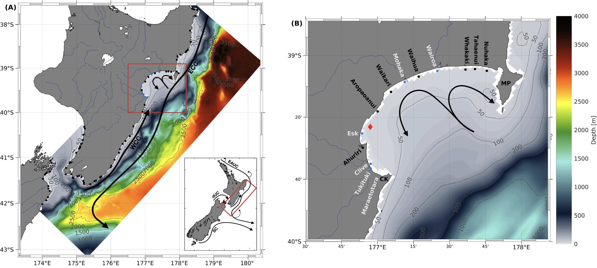
Figure 1. (A) Model domain showing bathymetry in meters. The red polygon shows the zoomed in area of Hawke’s Bay shown in (B). The inset in (A) shows the location of the model domain (red polygon) with respect to New Zealand. The black dots in (A, B) represent rivers with annual mean discharge and the cyan dots represent rivers with time-varying river discharge. The red diamond in (B) shows the location of the HAWQi buoy. ECC, East Cape Current; WCC, Wairarapa Coastal Current; EAUC, East Auckland Current; dUC, d’Urville Current; SC, Southland Current; CK, Cape Kidnappers; MP, Mahia Peninsula.

The large-scale circulation on the east coast of the North Island is dominated by two distinct ocean currents, the East Cape Current (ECC) and the Wairarapa Coastal Current (WCC; Figure 1A) (Chiswell et al., 2015; Stevens et al., 2019). The ECC, an extension of the East Auckland Current, transports warm, saline subtropical water southward offshore of the east coast of the North Island (Chiswell and Roemmich, 1998). The WCC, on the other hand, flows inshore of the ECC and transports cool, fresh water northward along the east coast of the North Island. The WCC occurs within 40–50 km from the coast and extends as far north as Mahia Peninsula (Chiswell, 2000). Historical temperature and salinity measurements collected in Hawke’s Bay, on the continental shelf outside the bay, and to the south of the bay, showed that temperature and salinity in the bay are lower compared to the shelf water along the open coast (Ridgway and Stanton, 1969). Based on these measurements, it was deduced that water in Hawke’s Bay is a mixture of oceanic water entering the bay from south of Cape Kidnappers and fresh water from river discharge. However, the characteristics and dynamics of these coastal buoyant outflows are still ill defined.

In the present study a high-resolution (2 km) hydrodynamic model is used to investigate the spatiotemporal variability of river plumes in Hawke’s Bay. In particular, Self-Organizing Maps (SOMs) are used to identify the dominant river plume patterns, linking them to potential control mechanisms (river discharge, bay-scale circulation, wind forcing). The hydrodynamic model, described in Section 2, spans the period 2013–2017 and includes realistic river discharge for six rivers discharging into Hawke’s Bay which enables us to evaluate the interannual variability of freshwater plumes in Hawke’s Bay.

2 Data and methods

2.1 Hydrodynamic model configuration

The Regional Ocean Modelling System (ROMS) was used to simulate the distribution and advection of freshwater plumes in Hawke’s Bay for the period 2013 to 2017. ROMS is an open source (www.myroms.org), three-dimensional, free-surface, terrain-following hydrodynamic ocean model widely used by the scientific community for a diverse range of applications including coastal circulation (e.g. Chao et al., 2018) and river plume dispersal and dynamics (e.g. Denamiel et al., 2013; Zhang et al., 2009). ROMS uses the hydrostatic and Boussinesq approximations to solve the three-dimensional Reynolds-Averaged Navier-stokes equations (Shchepetkin and McWilliams, 2005; 2009) on a horizontal curvilinear Arakawa C grid. It provides a flexible structure that allows multiple choices for many of the model components such as advection schemes, turbulence models and lateral boundary conditions.

2.1.1 Model domain, forcing and boundary conditions

The model domain covers the continental shelf of the eastern North Island of New Zealand extending from Cook Strait in the south to East Cape in the north (Figure 1). It has a horizontal resolution of ∼2 km with 30 stretched terrain-following vertical levels resulting in a vertical resolution of 0.5–3 m in Hawke’s Bay and 3–90 m offshore. The model bathymetry was constructed from various sources including the NIWA bathymetry database (https://niwa.co.nz/oceans/resources/bathymetry/download-the-data), land elevation data, regional coastline data obtained from Land Information New Zealand (https://data.linz.govt.nz), and the General Bathymetric Chart of the Oceans (GEBCO; https://www.gebco.net/) gridded ocean bathymetry.

The model was initialised on 1 January 2013 with initial and open boundary conditions for the hydrodynamic variables (velocity, temperature, salinity and sea surface height) derived from a global ocean analysis and prediction system based on the Hybrid Coordinate Ocean Model (HYCOM; Chassignet et al., 2009). HYCOM is forced with surface atmospheric forcing provided by the Navy Operational Global Atmospheric Prediction System (NOGAPS). It assimilates data from several sources, including along-track satellite altimetry observations, satellite-measured and in-situ surface temperature and vertical temperature profiles from XBTs, Argo and moorings. The HYCOM product used here provides daily snapshots of the 3-dimensional state of the global ocean on a 1/12° grid.

Tides were imposed at the boundaries of the model domain in terms of the amplitude and phase of 13 tidal constituents derived from the New Zealand tidal model described by Walters et al. (2001). The ROMS tidal forcing scheme uses the amplitude and phase of the tidal constituents to calculate the tidal sea surface height and depth-averaged velocity at each time step and adds them to the lateral boundary data.

At the open boundaries, a nudging layer (10 grid cells) was used to relax the model temperature, salinity and baroclinic velocities towards HYCOM. Weak nudging towards HYCOM was also applied in the interior of the model domain below ∼200 m to prevent it from drifting away from a realistic state. Flather (1976) and Chapman (1985) boundary conditions were imposed at the lateral open boundaries for the barotropic currents and sea surface height, respectively. Radiation conditions (Marchesiello et al., 2001) were used at the boundaries for baroclinic velocities and tracers (e.g. temperature, salinity).

The ROMS simulation is forced at the surface with heat, momentum and freshwater fluxes. The heat and freshwater fluxes were obtained from six-hourly NCEP/NCAR reanalysis data (Kalnay et al., 1996). The NCEP/NCAR reanalysis product provides global atmospheric fields at a 2.5° resolution. The surface heat flux is only prescribed as a boundary condition and there is no feedback from the ocean to the atmosphere heat flux forcing. Consequently, drifts in SST occur due to small but persistent errors in heat flux. To correct for this, a heat flux correction term was applied to the SST, nudging the model SST towards observed SST from the 1/4° daily National Oceanic and Atmospheric Administration (NOAA) optimum interpolation SST analysis (Reynolds et al., 2007). The heat flux correction prevents the modelled SST from drifting too far from reality due to any biases in the surface fluxes but has a negligible effect on the day-to-day variability. Surface wind stress was calculated from 3-hourly winds obtained from the 12 km New Zealand Limited Area Model (NZLAM; Lane et al., 2009). Wind fields from NZLAM were preferred over NCEP/NCAR because wind fields with higher spatio-temporal resolution have been shown to improve model fidelity especially in coastal areas (e.g. Fu and Chao, 1997; Schaeffer et al., 2011; Small et al., 2015).

2.1.2 Freshwater input

The major rivers draining into Hawke’s Bay were represented in the model as point sources of freshwater and each river was tagged with a passive dye tracer. The freshwater sources along with their input locations are listed in Table 1. The input locations for each of the rivers were obtained from the New Zealand River Environment Classification (NZ REC; Biggs et al., 1990; Snelder et al., 2010) and then converted into model grid locations, with adjustments to ensure each freshwater input is located on the model’s land-sea boundary.

Table 1

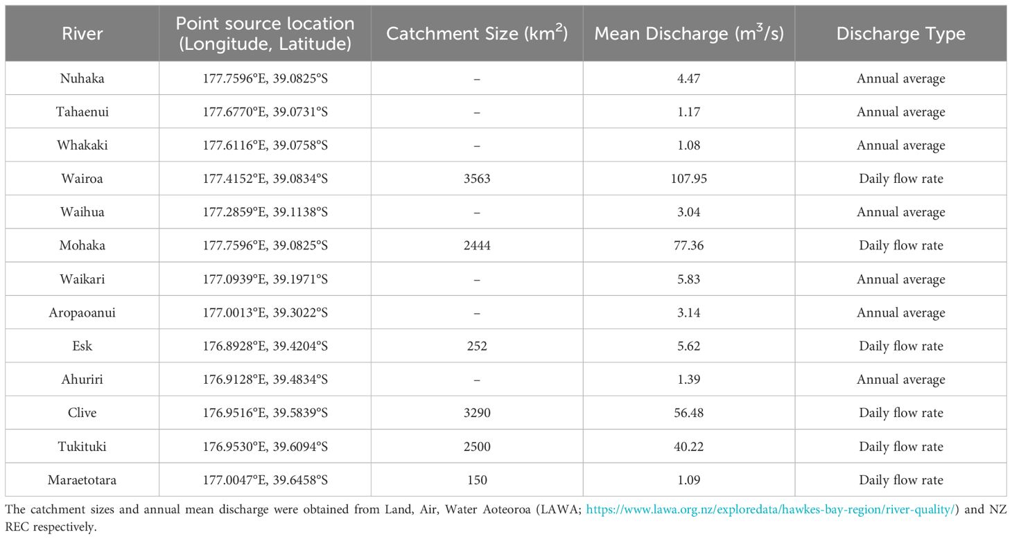
Table 1. Location, catchment size, mean discharge and type of discharge (annual average or daily flow rate) of freshwater point sources listed in order from north to south.

Daily discharges for six rivers discharging into Hawke’s Bay were obtained from the Hawke’s Bay Regional Council for the period 2013-2017 (Table 1). Data gaps exist in the daily discharge time-series however the portion of missing data tends to be small (10%). The k-Nearest Neighbour (kNN) imputation algorithm which replaces missing values in a dataset with the weighted mean value from a number (k) of nearby data points, was used in order to get a complete time-series for each of the six rivers. This algorithm has proven more effective than other imputation methods (e.g. Jadhav et al., 2019) but is sensitive to the value of k. A number of different k values were tested and for the river discharge data it was found that 6 was optimal as it did not change the average of the discharge time-series significantly (Supplementary Figure S1). An annual average flow obtained from the NZ REC was used for the rivers for which daily discharge measurements were not available. Even though all the major rivers are included as point freshwater sources, this study focuses on the six rivers with time-varying discharge. A similar simulation (not shown) run for one year with time-varying river discharge from four additional rivers show similar plume patterns to those presented here indicating that the contribution of these smaller rivers are minor.

The passive tracer computational capabilities of ROMS were used to track the freshwater discharges into Hawke’s Bay from the six rivers with time-varying discharge. To accomplish this, each river was tagged with its own conservative passive tracer (dye tracer) so that water coming in through each river has a dye concentration of 1 kg/m³. The tracer concentration has values between 0 and 1, and represents the concentration of the corresponding river freshwater, i.e. if the tracer has a value of 1 (100%) it means the water parcel is purely river water; if it has a value of 0 (0%) it means the water parcel contains no freshwater from that river. At the open boundaries, all six passive tracers are nudged to the ocean water (tracer is equal to zero) in the same manner as temperature and salinity.

Numerous coastal modelling (e.g. Gong et al., 2019; Johnson et al., 2024; Macdonald et al., 2023; Marta-Almeida et al., 2021) and observational (e.g. Feddersen et al., 2016; Houghton et al., 2009) studies have used dye tracers to study river plumes. However, as noted by Marta-Almeida et al. (2021), river discharge and dye concentration do not always exhibit a linear relationship due to additional sources and sinks of salinity in the ocean. Therefore, a water parcel with very low dye concentration may contain minimal freshwater, making it necessary to define a minimum reference dye concentration below which the dye can no longer be considered representative of riverine freshwater. Following Marta-Almeida et al. (2021), we use the 75th percentile of the cumulative dye tracer concentration to establish a minimum reference dye concentration of 0.1 (or 10%).

2.2 Model evaluation

The model was evaluated against satellite and in situ observations to establish that the modelled ocean hydrodynamics has acceptable fidelity. The model was assessed against high-resolution satellite sea surface temperature as well as against in situ temperature and salinity from a mooring in Hawke’s Bay. The latter is to demonstrate that the model is valid for evaluating the plume dynamics in Hawke’s Bay, while the former is to demonstrate the validity of the model in reproducing the far-field dynamics.

2.2.1 Satellite sea surface temperature

The spatial variability of the modelled sea-surface temperature (SST) was compared with the Multiscale Ultra-high Resolution (MUR) SST data set produced by the Group for High resolution Sea surface Temperature (GHRSST). This data set uses a Multi-Resolution Variational Analysis (MRVA) method to produce daily, gap-free gridded SST estimates from the 1 km MODIS SST observations combined with AVHRR, microwave and in situ SST (Chin et al., 2017).

2.2.2 In situ temperature and salinity

Temperature and salinity from the HAWQi (HAwke’s Bay Water Quality information) water quality buoy were obtained from the Hawke’s Bay Regional Council. The HAWQi water quality buoy, located approximately 5 km offshore in Hawke’s Bay (Figure 1B), collects continuous temperature and conductivity measurements at four depths (0.5 m, 5 m, 10 m, 15 m). This data, available intermittently for the 2015–2017 model period, was used to assess the model’s skill in reproducing the observed temperature and salinity in Hawke’s Bay at two depths, 0.5 m and 15 m.

2.2.3 Validation metrics

The skill of the model was assessed against the observational time-series data through statistical techniques such as the Pearson’s correlation coefficient and root-mean-square differences (RMSD). The RMSD and Pearson’s correlation coefficient were calculated using daily temperature and salinity data as follows:

$$RMSD={[\frac{1}{N}\sum {(M-O)}^2]}^{\frac{1}{2}}$$

$$Corr=\frac{1}{N}\sum \frac{(M-{\mu }_M)(O-{\mu }_O)}{{\sigma }_M{\sigma }_O}$$

where M and O are modelled and observed values of the variable, ${\mu }_M$, ${\mu }_O$, ${\sigma }_M$ and ${\sigma }_O$ are the temporal averages and standard deviations and N is the number of data points.

The model skill was further assessed using the statistical method developed by Willmott (1981)

$$WS=1-\frac{\langle {(M-O)}^2\rangle }{\langle {(|M-{\mu }_O|+|O-{\mu }_O|)}^2\rangle }$$

where angle brackets denote the time average and vertical bars denote absolute values. The Willmott skill parameter is a simple measure of the agreement between two data sets with WS =1 denoting perfect agreement and WS = 0 denoting complete disagreement.

2.3 Analysis

Although each of the six time-varying rivers was tagged with a distinct passive tracer, all analyses were performed using the cumulative tracer concentrations.

2.3.1 Empirical orthogonal function analysis

Empirical orthogonal function (EOF) analysis, a widely used analysis technique, was used to understand the spatial and temporal variability of the river plumes in Hawke’s Bay by applying it to the cumulative daily passive tracer concentration. EOF analysis is used to decompose a space- and time-distributed data set into a set of orthogonal modes that describe the covariability of the data set (Björnsson and Venegas, 1997). In the EOF decomposition, the percentage of variance of the data set explained by each mode is represented by the eigenvalue of that mode. A small number of modes generally captures most of the variance of the data set. EOF analysis is widely used to determine the spatio-temporal variability of river plumes. Lihan et al. (2008) and Chen et al. (2017) applied EOF analysis to satellite derived spectral reflectance to determine the spatio-temporal variability of the Tokachi and Pearl River plumes, respectively. Falcieri et al. (2014), on the other hand, applied EOF analysis to modelled sea surface salinity to determine the spatio-temporal variability of the Po River plume.

2.3.2 Self-Organizing Maps

The Self-Organizing Map (SOM) or Kohonen map (Kohonen, 1990; 2013), is a type of unsupervised, artificial neural network that is particularly adept at pattern recognition and classification. It maps multidimensional data onto a low-dimensional (usually 2-D) space while preserving the topological features of the original data. A detailed description of the SOM theory and algorithm is provided in Kohonen (1998; 2001), Richardson et al. (2003) and Liu et al. (2006a, 2006b). In the field of oceanography, SOM applications include SST and wind pattern extractions from satellite data (e.g. Richardson et al., 2003), identification of vertical chlorophyll profiles from in-situ fluorescence profiles (Silulwane et al., 2001), and the identification and prediction of river plumes (e.g. Falcieri et al., 2014; Lu et al., 2022).

The results obtained from a SOM analysis are sensitive to the set of user-defined parameters which include the number of neural network nodes (i.e. map size), the lattice structure (rectangular vs hexagonal), neighbourhood size and learning rate. A smaller number of neural network nodes (i.e. smaller map size) will result in more general patterns while a larger number of nodes will result in more detailed patterns.

In this study, the SOM was applied to the passive tracers as a means to extract the different river plume patterns that form in Hawke’s Bay under different environmental conditions (river discharge, wind and ocean currents). The SOM was applied to all passive tracers combined as well as to passive tracers associated with the individual rivers; however, only the former is presented here. Sensitivity tests revealed no significant difference between a rectangular and hexagonal lattice structure of the SOM applied to the passive tracers (see Supplementary Figure S2). Additional sensitivity tests also showed that a four-node (2 x 2) SOM best summarises the variability of plume patterns in Hawke’s Bay. A higher number of nodes (e.g. 3 x 3) produced a greater number of patterns, many which were similar in structure (Supplementary Figure S3). Thus, we opted for a SOM with a 2 x 2 rectangular lattice structure with a neighbourhood size of 3 and a high number (1000) of training iterations. Based on the SOM analysis the four river plume patterns identified can be related to other associated variables such as currents and river discharge by aggregating and averaging the variables associated with each pattern.

3 Results

3.1 River discharge variability

A number of high discharge events occurred throughout the 2013–2017 period, most of which where experienced, to different degrees, by all rivers at roughly the same time (Figure 2). The cumulative annual mean discharge was greatest in 2017 (361.60 m³/s) owing to a number of large discharge events. A single high discharge event occurred in 2015 across all rivers resulting in the smallest cumulative annual mean discharge (229.16 m³/s). The river discharge of all six rivers show a similar seasonal cycle with higher discharges in winter (JJA) compared to summer (DJF). The cumulative river discharge displays a maximum discharge of 579.26 m³/s in September and a minimum discharge of 81.72 m³/s in January (not shown).

Figure 2

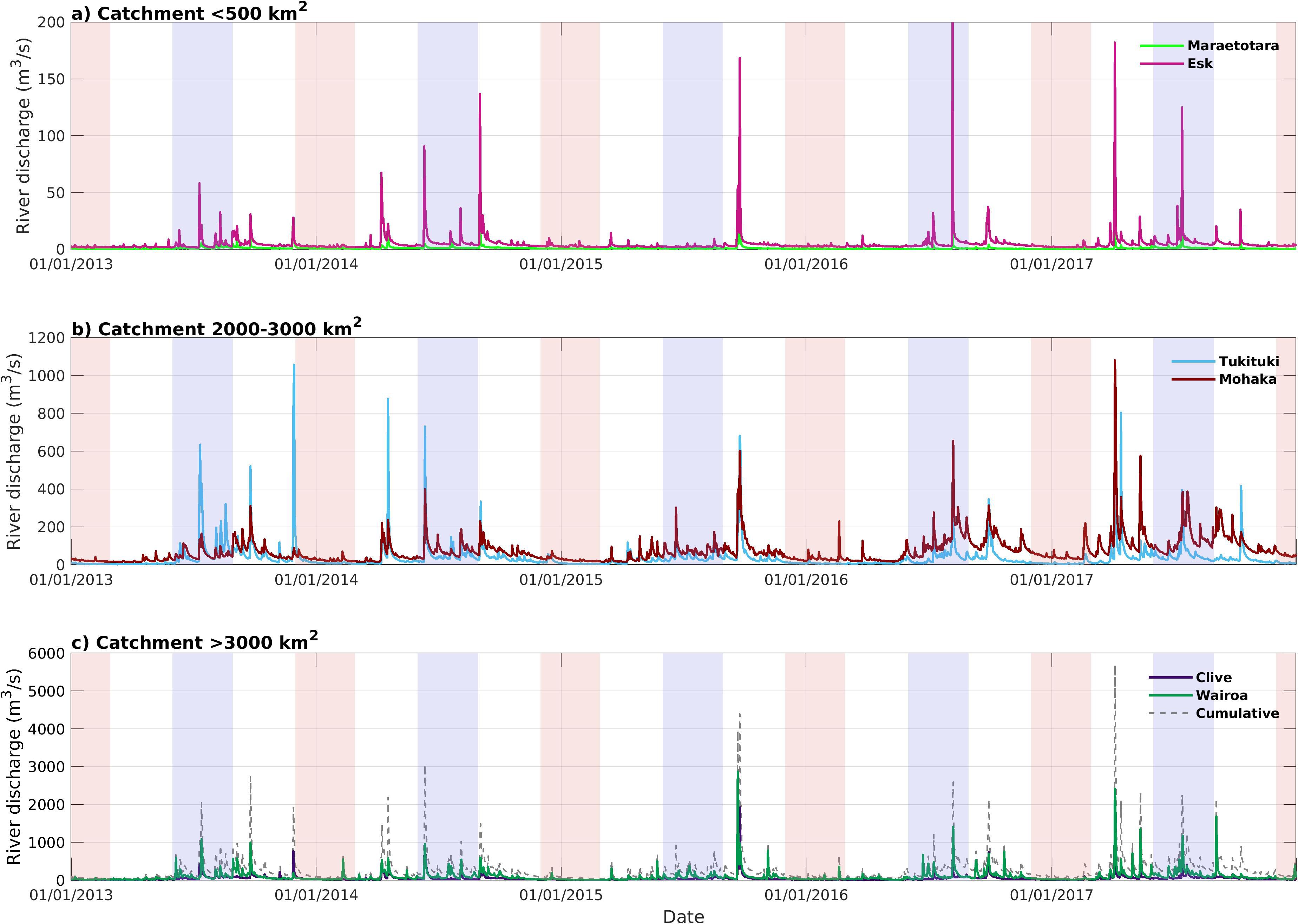
Figure 2. Time-varying river discharge for six rivers discharging into Hawke’s Bay. Different rivers are grouped together based on catchment size obtained from Land, Air, Water Aoteoroa (https://www.lawa.org.nz/explore-data/hawkes-bay-region/river-quality/). The grey dashed line in (c) denotes the cumulative river discharge from the six rivers. Red shading denotes summer months (DJF), while blue shading indicates winter months (JJA). Note the differences in scale between (a–c).

3.2 Model-data comparison

The overall distribution of mean SST is reasonably captured in the model (Figures 3A, B) with a cold bias in the northern part of the domain and a predominantly warm bias throughout the southern part (Figure 3D). Overall, biases are small with magnitudes of less than 1°C, which is small compared to the large variability (greater than 1°C) observed in the satellite SST for this region (Figure 3C). The model reproduces the north-south gradient of SST as is observed in the satellite SST (Figures 3A, B). However, in the model, warmer SST, associated with the ECC, extends further south and is shifted closer to the coast. As a result, the Wairarapa Coastal Current, signified by the cold SST along the southeast coast of the North Island, is narrower and warmer in the model (Figure 3B). In Hawke’s Bay, this study’s focus area, the model compares favourably against the satellite SST. The model reproduces the cross-shelf gradient of SST as is observed in the satellite SST with colder temperatures (16-16.5°C) in Hawke’s Bay and warmer temperatures (>16.5°C) offshore (Figures 3A, B). There is a slight (<0.5°C) overestimation of SST throughout most of the bay (Figure 3D) but this is less than the satellite SST standard deviation in the bay (Figure 3C).

Figure 3

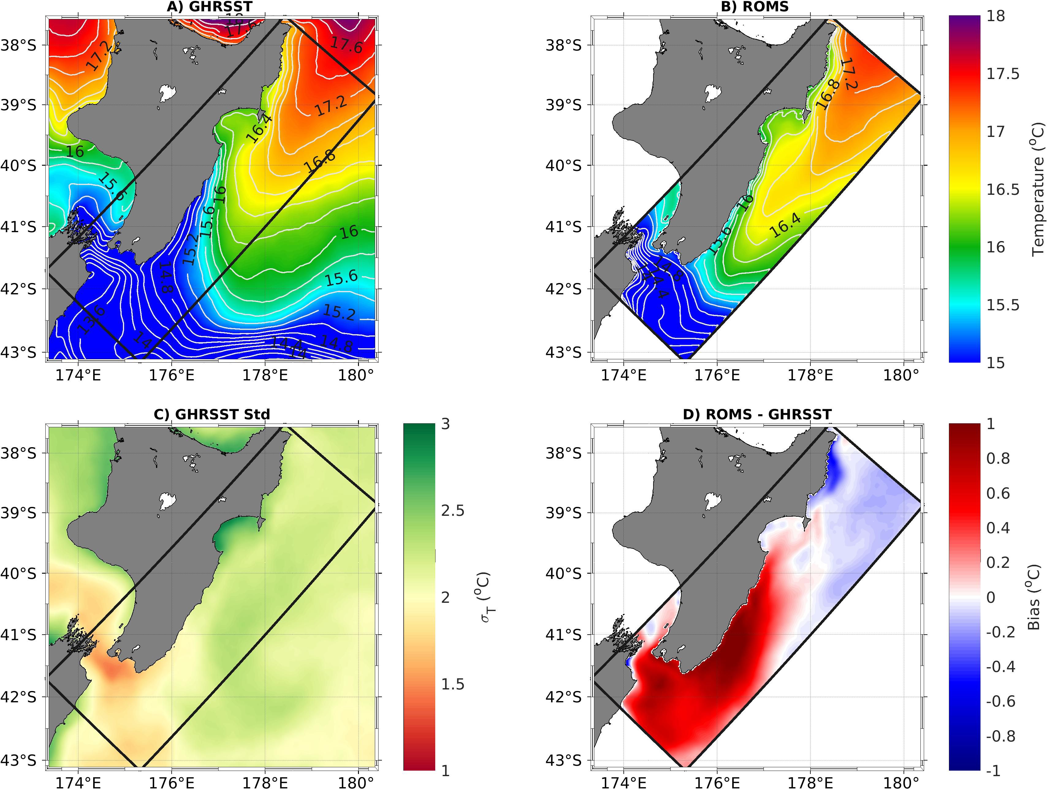
Figure 3. Comparison of satellite-derived (A) and modelled (B) 4-year (2013-2017) mean sea surface temperature. (C) Standard deviation of the satellite-derived SST and (D) model bias (model SST - satellite-derived SST). The black rectangle indicates the model domain.

The comparison between model-simulated and in situ temperature and salinity indicates that the model simulates a realistic temperature and salinity field in Hawke’s Bay (Figure 4; Table 2). The model has high predictive skill (WS>0.95) for both surface (0.5 m) and subsurface temperature (15 m). However, the predictive skill for salinity is lower (WS<0.8).

Figure 4

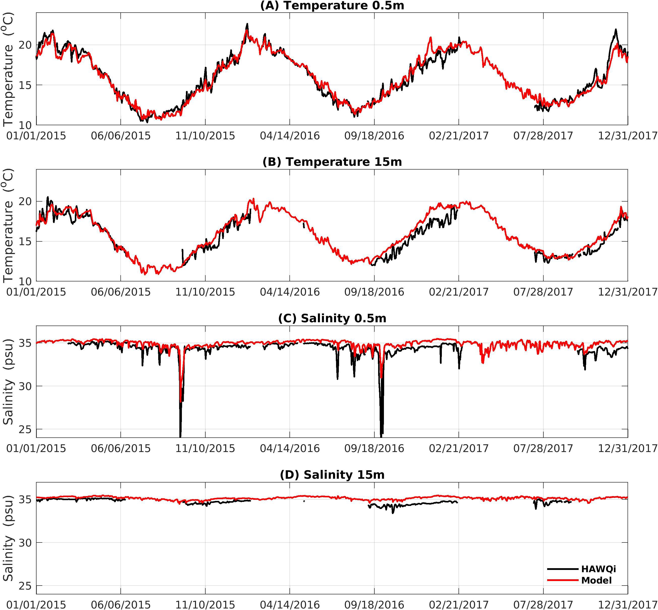
Figure 4. Modelled (red) and observed (black) temperature (A, B) and salinity (C, D) at 0.5 m and 15 m depth. The observed data are from the HAWQi buoy.

Table 2

Table 2. Summary of the validation metrics for temperature and salinity at 0.5 m and 15 m depth of the model simulation compared to observed data.

The high correlation coefficients (r >0.9) and low RMSE values (RMSE < 0.9°C) for temperature (Table 2) indicate that the model realistically simulates the observed seasonal cycle with higher temperatures in summer and lower temperatures in winter (Figures 4A, B). In addition, the model also has reasonable skill in simulating short-term fluctuations. The lower correlation coefficient and higher RMSE of subsurface temperature compared to surface temperature (Table 2) indicates that the model is less skilful in representing subsurface temperatures. The improved skill of the model in representing surface temperatures can, in part, be attributed to the nudging of SST to observed SSTs as described in Section 2.1.1. However, the high predictive skill for subsurface temperatures indicates that the fidelity of the model is not purely an artefact of nudging.

The winter of 2015 was the coldest winter on record and this is reproduced in the model (Figures 4A, B). The observed surface (0.5 m) temperature during the austral summer of 2015/2016 and 2017/2018 had noticeably higher temperatures (>21°C) which are also evident in the model, however the model underestimates the amplitude of these events. The higher temperatures during the summer of 2015/2016 and 2017/2018 can be attributed to marine heatwaves occurring in Hawke’s Bay (Madarasz-Smith and Shanahan, 2020). The 2017/2018 marine heatwave coincides with a coupled ocean-atmosphere heatwave that occurred in the New Zealand region during the austral summer of 2017/2018 (Salinger et al., 2019). This heatwave was the most intense on record and resulted in sea surface temperature anomalies of around 2°C across the entire Tasman Sea/New Zealand region (Salinger et al., 2019).

The model-simulated salinity performs well against the observed salinity, albeit with lower skill scores and correlation coefficients than temperature (Figure 4; Table 2). As with temperature, the model is less skilful in representing subsurface salinity compared to surface salinity. In general, the model tends to over-estimate surface and subsurface salinities (Figures 4C, D). The modelled salinity accurately predicts the timing of low salinity events such as those observed in 2015 and 2016 in response to high river discharge events, however it underestimates the amplitude of these events. High discharge events in 2015 and 2016 reduced surface salinity by ∼10 psu, whereas the model predicts a decreases of about 6 psu and 4 psu for 2015 and 2016, respectively (Figure 4C) The over-estimation of the modelled salinity can, in part, be attributed to an overestimation of salinity in the HYCOM boundary conditions which also does not reproduce the low salinity events (not shown).

3.3 Plume characteristics and drivers

3.3.1 Mean plume characteristics

The time-averaged (2013-2017), depth-integrated passive tracer concentration (Figure 5A) from all six tracers combined reveals the typical dispersal patterns of freshwater in Hawke’s Bay. The freshwater inflow into Hawke’s Bay forms a well defined region of freshwater influence (ROFI), defined here as the region where freshwater concentration exceeds 10% (white contour in Figure 5A), that follows the coast and spreads throughout the bay.

Figure 5

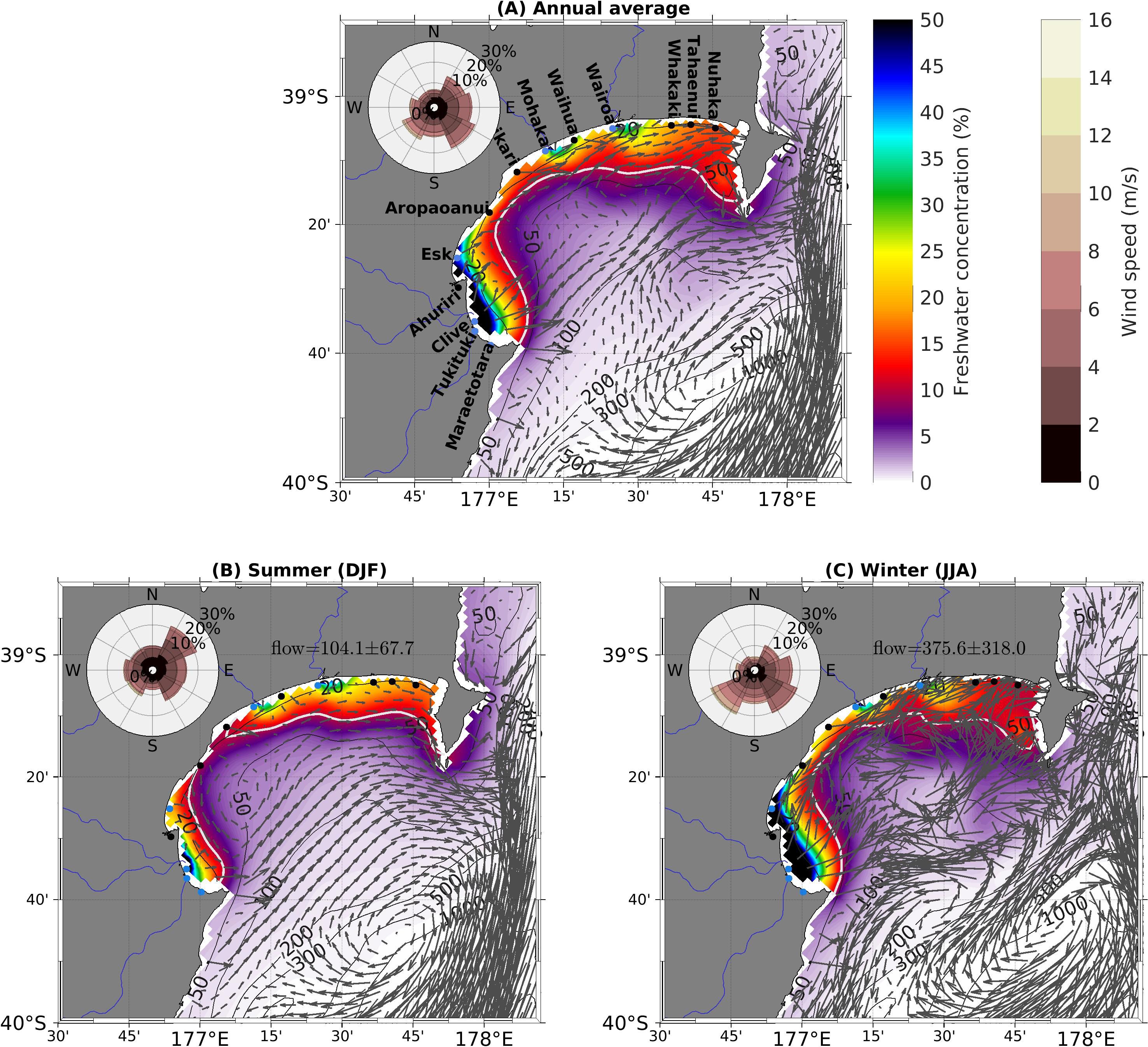
Figure 5. (A) Time-averaged (2013-2017) and seasonal mean dye concentration (colour), currents (grey vectors) and wind (wind roses) for (B) summer (DJF) and (C) winter (JJA) in Hawke’s Bay. The seasonal mean and standard deviation of river discharge is also indicated on (B, C). The white contour denotes freshwater concentrations of 10%. Grey contours denote the model bathymetry in meters.

Distinct plumes of high freshwater concentrations are associated with the six rivers under consideration here: the Wairoa, Mohaka, Esk, Clive, Tukituki and Maraetotara rivers. The most distinct plume of freshwater occurs in the southern Hawke’s Bay where there is a confluence of freshwater plumes from four (Mareatotara, Tukituki, Clive and Esk) of the six rivers. Freshwater is transported northward in a narrow band along the coast and concentrations tend to remain high inshore of the 50 m isobath, decreasing as it is advected within and out of Hawke’s Bay.

The ROFI covers, on average, an area of 1439.81 km² and extends up to ∼88 km from the coast. The southern Hawke’s Bay ROFI, consisting of freshwater inflow from the Maraetotara, Tukituki, Clive and Esk Rivers, makes up ∼40% of the entire ROFI, extending across an area of 563.96 km².

On average, two distinct ROFI form in Hawke’s Bay during summer: one in southern Hawke’s Bay extending from the Maraetotara River to the Aropaoanui River with the highest concentration of freshwater centred around the Clive River, and a second in northern Hawke’s Bay extending from the Waikari River to Mahia Peninsula (Figure 5B). Together these two ROFI cover an area of 999.86 km² with the southern ROFI extending across an area of 283.98 km². The ROFI that forms during winter resembles the time-averaged ROFI (Figure 5A) with a single ROFI extending from Cape Kidnappers in the south to Mahia Peninsula in the north, extending over an area of 1383.82 km². The similarity between the time-averaged ROFI and winter-time ROFI can be attributed to higher freshwater discharges in winter, generating larger river plumes, which dominates the time-averaged pattern.

3.3.2 Spatio-temporal variability

The spatial extent of the ROFI in Hawke’s Bay shows considerable temporal variability ranging from as small as ∼100 km² to ∼3484 km² [25 days after biggest river discharge (Figure 6)]. The area of the ROFI is positively correlated (R = 0.7) with total river discharge at a lag of 7 days which represents the time taken for riverine water to disperse within the bay. In addition, prevailing negative cross-shelf (onshore) and positive alongshore (northward) wind stress over Hawke’s Bay act together to modulate the spatial extent of the ROFI (Figure 6B).

Figure 6

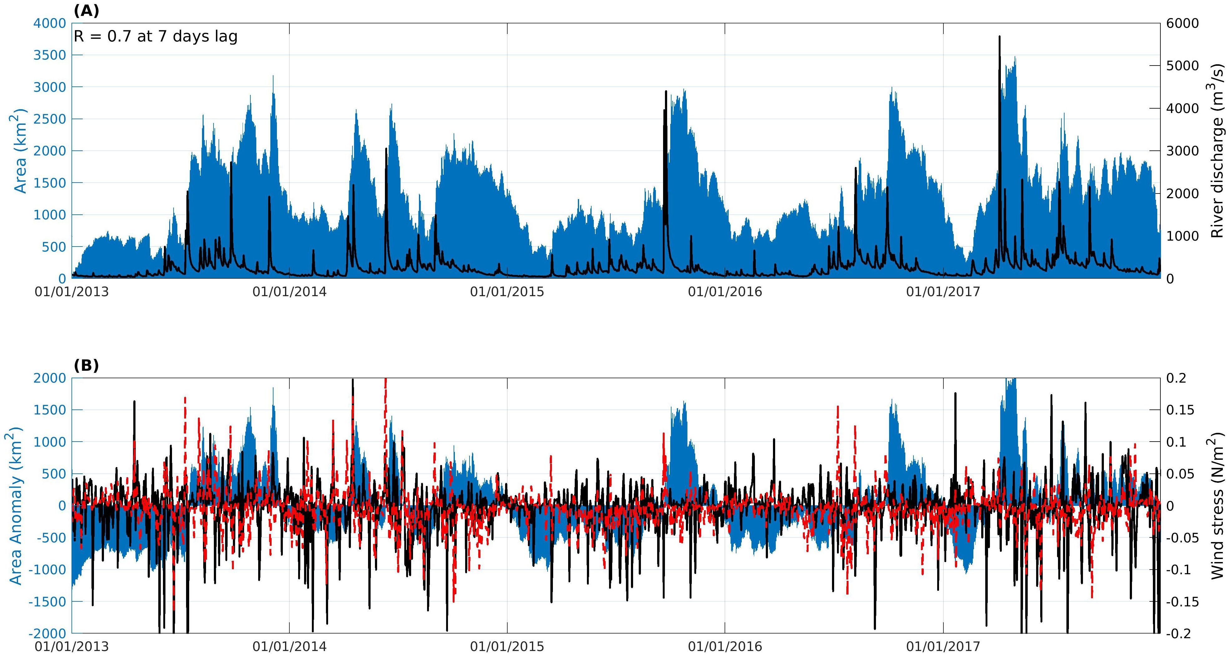
Figure 6. (A) Time-varying cumulative plume area based on a dye concentration of 10% (blue bars) and cumulative river discharge (black line). (B) Plume area anomaly - calculated as the difference between the daily cumulative plume area and the time-averaged plume area - and alongshore (black line) and cross-shelf (dashed red line) wind stress.

The ROFI area anomaly - defined as the difference between the daily spatial extent and the time-averaged spatial extent - reveals prolonged periods (>2 months) of both below- and above-average ROFI extent (Figure 6B). Negative anomalies typically occur in summer, coinciding with low river discharge, while positive anomalies are more common in winter, aligning with periods of high river discharge.

Prolonged periods (>2 months) of above-average ROFI extent followed high river discharge events in 2015, 2016 and 2017. The enlarged ROFI observed in 2015 and 2016 was primarily a result of substantial freshwater input and prevailing cyclonic alongshore circulation, with a secondary contribution from wind forcing. During these periods, weak (<0.05 N/m²) negative alongshore and cross-shelf wind stress enhanced the alongshore advection of freshwater by reinforcing the cyclonic alongshore currents. At the same time, the weak negative cross-shelf wind stress was unlikely to significantly inhibit offshore spreading of the plume. In contrast, the positive area anomaly observed in 2017 coincided with predominantly weak negative cross-shelf wind stress and strong (>0.05 N/m²) positive alongshore wind stress. Similar to the anomalies in 2015 and 2016, the weak negative cross-shelf wind stress likely had minimal influence on offshore advection of freshwater, while the strong alongshore wind stress significantly enhanced the alongshore transport of river plumes.

An EOF analysis of the dye tracer concentration was conducted to identify the dominant spatial patterns of plume variability. Emphasis is placed on the first two EOF modes, which together explains 62.1% of variability in dye concentration. The first mode, explaining ∼52.1% of the overall variability (Figure 7A), shows a single-signed pattern across Hawke’s Bay. The spatial pattern of the first EOF mode, showing high variability in the coastal region, closely resembles the time-averaged ROFI pattern with a distinct bulge in southern Hawke’s Bay and a well extended coastal plume that spreads along the coast. The majority of the variance (>40%) explained by this mode is concentrated in the nearshore region of southern Hawke’s Bay, decreasing both alongshore and cross-shore. Notably, this mode accounts for 70-85% of the variance in southern Hawke’s Bay in the vicinity of the plume generated by the southernmost rivers. The principle component of the first mode (PC1) indicates high temporal variability (Figure 7C) and shows an inverse correlation with the total river discharge. This inverse relationship arises because large discharge events produce more extensive, but diluted freshwater plumes in the bay, while low discharge events lead to more concentrated plumes. The correlation coefficients between PC1 and the daily discharge show maximum inverse correlation (r=0.56) at zero days lag and the correlation coefficient decreases with increasing lag and lead times (Figure 7D). This implies that there is a near immediate response in the freshwater concentration in the bay to the variation of the discharge from the Hawke’s Bay river network.

Figure 7

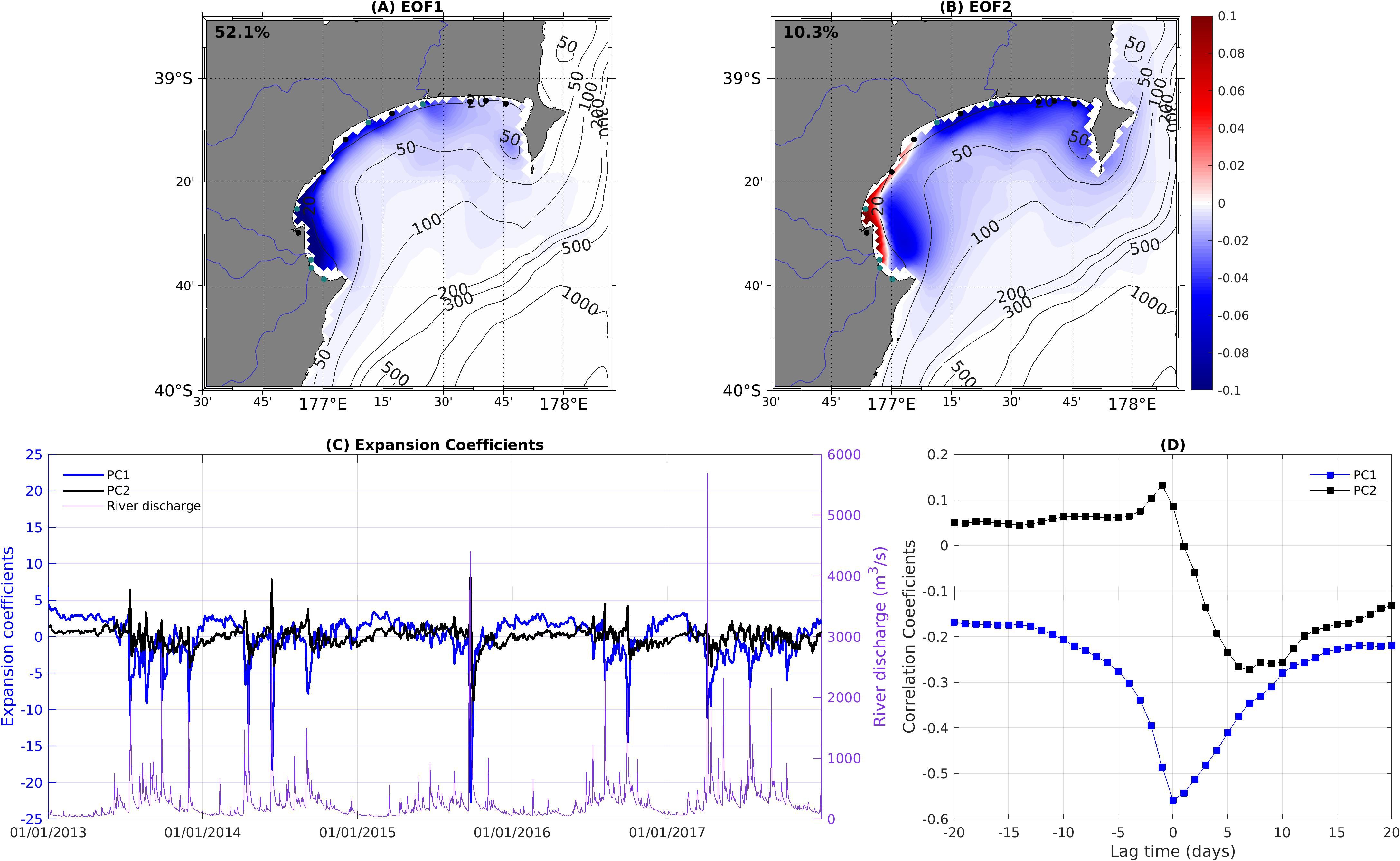
Figure 7. Spatial pattern of the 1st (A) and 2nd (B) EOF mode of the modelled dye tracer concentration. The explained variance of each mode is shown in the left corner. (C) The expansion coefficients of the 1st (blue) and 2nd (black) EOF modes along with the time-series of total river discharge (purple). (D) The correlation coefficients between the two expansion coefficients and the river discharge at different lags.

The second EOF mode explains about 10% of the variance and exhibits an out-of-phase relationship between the ROFI in the south and the north (Figure 7B). The EOF displays positive values inshore of the 20 m isobath in the south and negative values offshore as well as in the north (inshore and offshore). This mode represents a pattern in which the plumes from the south are advected northward while the plumes in the north are advected southward. Similar to the first mode, the principal component of the second mode (PC2) exhibits high temporal variability (Figure 7C). When PC2 is positive (negative), there is an intensification (reduction) of dye concentration in the nearshore region between the Esk and Tukituki rivers and a reduction (intensification) across the rest of the bay. PC2 is weakly correlated with total discharge (Figure 7D) indicating that this pattern is not strongly modulated by river discharge. Additionally, both PC1 and PC2 exhibit weak (r <0.3) correlation with alongshore and cross-shelf wind stress (not shown), suggesting that horizontal plume patterns are only minimally influenced by wind forcing - consistent with the inference for the positive area anomalies observed 2015, 2016 and 2017.

3.3.3 SOM analysis

EOF analysis is capable of extracting the most common patterns but lacks the ability of finding the least occurring or nonlinear patterns since it reduces most of the variability to the first few modes (Björnsson and Venegas, 1997). An alternative representation of the different patterns of ROFI in Hawke’s Bay, even less frequent ones, can be obtained with the Self-Organizing Map. SOM are increasingly being used for classifying and identifying patterns and their frequencies on the base of the data topology rather than the variance. The SOM analysis, as explained in Section 2.3.2, provides a more detailed representation of the ROFI patterns in Hawke’s Bay which may not be captured by the EOF analysis.

The river plume variability in Hawke’s Bay is best described by four patterns (Figure 8). The first plume type (hereafter referred to as Pattern I), occurring 45.9% of the time (Figure 8A), closely resembles the summer average (Figure 5B) and features a prominent northern ROFI and smaller southern ROFI, separated by a cyclonic eddy. In addition, the northern ROFI is associated with north-eastward and eastward alongshore flow, while the southern ROFI is associated with eastward and south-eastward currents associated with the eddy. Pattern I tends to be associated with low river discharge. The average river discharge associated with this pattern is ∼110 m³/s whereas the average cumulative river discharge over the entire time-series (2013-2017) is ∼266 m³/s. The winds associated with Pattern I are predominantly weak (<10 m/s), downwelling-favourable south-easterlies associated with prevailing negative cross-shelf (onshore) and positive alongshore (southward) wind stress. Although weak alongshore currents allow for some alongshore advection of river plumes, they limit the extent of alongshore transport. In combination with downwelling-favourable winds and the cyclonic circulation feature in southern Hawke’s Bay, these factors help maintain the separation between the northern and southern ROFIs.

Figure 8

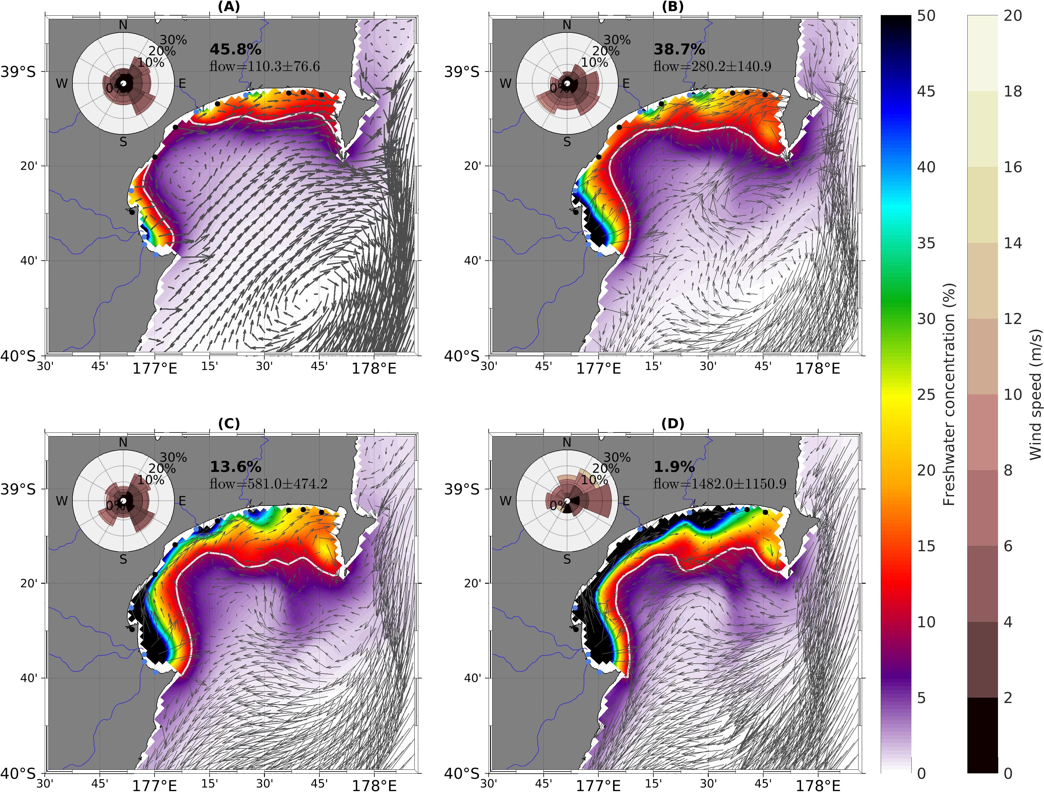
Figure 8. Hawke’s Bay river plume patterns I - IV (A-D) as delineated by Self-Organising Map (SOM) from modelled passive tracer concentrations. The vectors illustrate the surface currents associated with each SOM pattern while the wind roses indicate the spatially averaged wind patterns. The mean and standard deviation of river discharge (m³/s) associated with each pattern along with the appearance percentage is shown on each of the panels.

The second ROFI pattern (Pattern II; 38.4% occurrence) (Figure 8B) strongly resembles the annual and winter averages (Figures 5A, C) and consists of a more continuous and wider ROFI compared to Pattern I. Pattern II is associated with slightly higher river discharge (∼280 m³/s) and stronger alongshore currents (8–10 cm/s compared to 7–9 cm/s for Pattern I) across most of the ROFI. This pattern also shows higher freshwater concentrations off Mahia Peninsula (∼177.8°E, 39.2°S) that is associated with a cyclonic eddy. The winds associated with Pattern II are predominantly downwelling-favourable south-westerlies and south-easterlies. Stronger alongshore currents, driven by intensified south-westerly and south-easterly winds, enhance the alongshore advection of river plumes, leading to the formation of a single, larger ROFI.

The third (13.6% occurrence; Figure 8C) and forth (1.9% occurrence; Figure 8D) plume types (Pattern III and IV, respectively) also consists of a continuous ROFI. However, in Pattern III the ROFI extends further offshore in the northern and southern part of Hawke’s Bay compared to Pattern IV. In addition, the strong plume in the south extends northward forming a continuous ROFI with the plumes generated off the Mohaka and Wairoa rivers. Pattern III is associated with higher river discharges (∼580 m³/s) and cyclonic alongshore circulation which advects the individual river plumes northwards. The winds associated with this pattern are predominantly downwelling-favourable south-easterlies. The increased freshwater input associated with this pattern produces larger individual river plumes, which are advected alongshore by cyclonic currents driven by downwelling-favourable winds. It also results in a continuous, narrow, coastal band of high freshwater concentration.

The fourth and least frequent plume type (Pattern IV) consists of a single ROFI along the coasts that extends northward from Cape Kidnappers to well past the Wairoa River (Figure 8D). This pattern is associated with extremely high river discharge (∼1507 m³/s) and strong northward alongshore flow (20–30 cm/s) between the Tukituki and Mohaka rivers and southward alongshore flow (10–20 cm/s) from Mahia Peninsula to the Wairoa River. The winds associated with Pattern IV are predominantly weak (0–6 m/s) easterlies and strong (6–14 m/s) north-easterlies. The extreme freshwater input associated with this pattern generates large individual river plumes which, combined with the bidirectional alongshore currents, lead to the formation of a single, expansive ROFI. Upwelling-favourable winds further contribute to its spatial extent by enhancing offshore advection. Similar to Pattern II, both Pattern III and IV show higher freshwater concentrations off Mahia Peninsula that is associated with a cyclonic eddy. However, in the latter two types the eddy is stronger resulting in more freshwater entrainment.

4 Discussion

A statistical approach applied to a realistic 3D hydrodynamical model with passive tracers representing riverine water was used to describe the plume patterns generated in Hakwe’s Bay. In addition, the plume patterns were also linked to potential drivers such as river discharges and winds. The hydrodynamic model was forced with realistic surface forcing, tides and freshwater input from all of the main rivers terminating in Hawke’s Bay.

The model was evaluated against high-resolution satellite derived SST as well as in situ time series of temperature and salinity measured in the bay. The comparisons show that the model realistically simulates the larger scale circulation, namely the East Cape Current and the Wairarapa Coastal Current as well as the bay-scale dynamics. In particular, the comparison with in situ measurements show that the model realistically captures the timing of events (e.g. heatwaves) even if the amplitudes of these events are underestimated.

4.1 Plume characteristic

The freshwater from six rivers draining into Hawke’s Bay form a well defined ROFI that is primarily confined inshore of the 50 m isobath and extends, on average, across approximately 50% of the bay (Figure 5). The limited spatial extent of the ROFI can, in part, be attributed to the prevailing south-easterly (downwelling-favourable) winds which impedes the offshore advection of freshwater plumes but promotes the alongshore transport through enhanced cyclonic currents. The two northern rivers, the Wairoa and Mohaka, contributes the most (∼60%) to the ROFI. These two rivers have some of the largest catchment areas and highest average discharge values (Table 1). Thus, as some of the largest contributors of freshwater to Hawke’s Bay it is expected that they would contribute significantly to the ROFI.

River discharge is the primary driver of seasonal variability of plumes generated by large (e.g. AmazonOrinoco plume (Da and Foltz, 2022), Po river plume (Falcieri et al., 2014) and small rivers (Korshenko et al., 2023) in other parts of the world. Similarly, the combined plume that forms in Hawke’s Bay shows strong seasonal variability linked to river discharge variability. The first mode of the EOF analysis (Figure 7), explaining more than 50% of the variability, closely resembles the time-averaged and mean winter ROFI pattern (Figure 5). In winter, a single ROFI extends across almost half the bay whereas in summer two distinct ROFI, a northern and southern, are formed which, together, extends across ∼30% of the bay. The seasonal difference observed in the areal extent can, primarily, be attributed to seasonal differences in river discharge.

Winter is characterised by higher average river discharge as well as more variable discharge (375.58 ± 317.99 m³/s) compared to summer (104.07 ± 67.74 m³/s). In addition, high discharge events (discharge > 1000 m³/s) are more prevalent in winter compared to summer. A higher mean river discharge in winter along with more high discharge events results in larger individual river plumes and an overall larger areal extent in winter compared to summer. The inverse correlation of the principle component with river discharge (Figure 7D) indicates that high discharge events characteristic of winter result in more extensive but diffuse freshwater plumes whereas low discharge events result in more concentrated freshwater plumes.

Although the weak correlation between the principle components from the EOF analysis and wind stress suggest a limited influence of wind on freshwater concentration, winds, especially seasonal differences, still play a role in shaping the spatial extent of river plumes in Hawke’s Bay. Prevailing south-westerly winds during winter, which are downwelling-favourable, drive strong cyclonic alongshore currents that enhance the alongshore advection of freshwater while limiting offshore spreading (Figure 5C). In contrast, north-easterly (upwelling-favourable) winds in summer weaken the opposing alongshore currents, thereby reducing the alongshore transport of freshwater (Figure 5B). Additionally, a cyclonic circulation feature in southern Hawke’s Bay helps maintain the separation between the northern and southern ROFIs, resulting in an overall smaller ROFI during summer compared to winter.

The extreme low salinity events (salinity <30 psu) observed in 2015 and 2016 in the WRIBO dataset provides further examples of the influence of wind on the spatial extent of freshwater plumes in Hawke’s Bay at longer timescales. The large discharge events resulting in the low salinity resulted in very large freshwater plumes with total plume areas exceeding the average area of ∼1300 km² by more than 1000 km² for up to a month (Figure 6B). The above average freshwater discharges experienced by the southernmost rivers (Clive, Esk and Tukituki) combined with strong offshore currents, generated a large freshwater bulge in southern Hawke’s Bay. Strong cyclonic alongshore currents aided with the northward advection of the southern plume to coalesce with the plume associated with the Wairoa and Mohaka rivers as seen for Pattern III (Figure 8C). The prevailing offshore (negative) cross-shore wind-stress facilitated the offshore transport of freshwater into Hawke’s Bay contributing to the above normal areal extent.

At shorter timescales (days to weeks), the response of freshwater plumes to river discharge variability is more varied with some plumes responding immediately to variations in discharge (Mendes et al., 2014; Fernández-Nóvoa et al., 2015) whereas others have a more delayed response (Fernández-Nóvoa et al., 2017; Chen et al., 2017). The strong correlation between the expansion coefficient of the first EOF and cumulative river discharge at zero lag (Figure 7D) indicates that there is an immediate response in the freshwater concentration of the plumes related to variations in discharge. However, the lagged correlation between the time-varying cumulative areal extent of the freshwater plumes generated in Hawke’s Bay and cumulative river discharge (Figure 6) indicates that the areal extent of freshwater plumes in the bay do not respond immediately to variations in discharge, instead the response time of the ROFI spatial extent to discharge from the river network is ∼1 week. This lagged response time in the ROFI spatial extent to changes in river discharge is likely due to greater retention of freshwater in the nearshore region as a result of weak nearshore currents. A similar response time was reported for the ROFI generated in the Firth of Thames/Hauraki Gulf, New Zealand (O’Callaghan and Stevens, 2017) as well as the Pearl River plume (Chen et al., 2017). For the Firth of Thames ROFI, the lagged response time was attributed to weak current speeds (O’Callaghan and Stevens, 2017).

4.2 Plume coalescence

Warrick and Farnsworth (2017), using physical scaling relationships of coastal watersheds and their buoyant plumes along with idealized modelling, postulated that 1) coastal margins with numerous small rivers (catchment size <10–000 km²) were more likely to have coalescing river plumes than coastal settings with large catchment areas (>100–000 km²) and 2) irregularly spaced river mouths that places some plumes relatively close to each other with respect to their size will result in more regular coalescence. The rivers terminating in Hawke’s Bay fit both of these criteria: all the rivers terminating in Hawke’s Bay have catchment sizes <5–000 km² and the rivers are irregularly and closely spaced (Figure 1; e.g. ∼40 km between Esk and Mohaka rivers, <4 km between Tukituki and Clive rivers). Additional factors such as coastal circulation, wind and river discharge also play an important role in plume coalescence (Mendes et al., 2016; Saldías et al., 2012, 2016; Warrick and Farnsworth, 2017).

Distinct plumes are associated with each of the individual rivers draining into Hawke’s Bay. The rivers in southern Hawke’s Bay (the Clive, Tukituki and Maraetotara rivers) are located in close proximity to each other compared to the rivers in northern Hawke’s Bay (the Wairoa and Mohaka). Thus, when plumes turn left due to wind and rotational forcing they merge forming a single plume that propagates northward (i.e. in the direction of Kelvin Wave propagation). The coalescence of river plumes in southern Hawke’s Bay is evident in all four SOM patterns (Figure 8) indicating that coalescence of these plumes are persistent and occurs under a range of environmental conditions. Therefore, it can be surmised that the close proximity of the rivers is the primary cause of the coalescence. The consolidated plume forming in southern Hawke’s Bay frequently merges with the plume generated at the mouth of the Esk River located slightly further north. This merger tends to occur under high discharge conditions and/or when northward alongshore currents dominate in the southern part of Hawke’s Bay. The northward elongation of the southern ROFI is facilitated by the prevailing positive alongshore wind stress (downwelling-favourable wind), which drives northward alongshore advection. The plumes generated by the two northernmost rivers, the Mohaka and Wairoa, also coalesce but only under high discharge conditions and is a result of larger plumes associated with each of the rivers along with alongshore plume advection by winds and currents. On rare occasions, opposing alongshore currents in northern and southern Hawke’s Bay advect the northern and southern plumes towards each other resulting in a single extensive ROFI as seen in Pattern IV from the SOM analysis (Figure 8D). The bidirectional advection of plumes in Hawke’s Bay tend to occur under upwelling-favourable conditions. Coalescence of the northern and southern plumes can also occur when high discharge conditions coincide with strong unidirectional along-shore currents (Figures 5C, 8C). Under these conditions the large plume generated in southern Hawke’s Bay is advected northward by strong, wind-enhanced alongshore currents to merge with the northern plume. Weak unidirectional alongshore currents accompanied by weak positive or negative alongshore wind stress, on the other hand, resulting in weak alongshore advection act to keep the northern and southern plumes separate (Figures 5B, 8A).

River plume coalescence have been observed for a number of other systems from remote sensing data (Saldías et al., 2012, 2016) and numerical modelling (Mendes et al., 2016; Gong et al., 2019) and suggest that coalescence mainly occurs during high discharge and downwelling-favourable conditions. Mendes et al. (2016) noted that plume interaction between the Douro River and Minho River along the Western Iberian coast only occurs under downwelling-favourable winds and as such is unidirectional with the Douro River plume merging with the upstream Minho River plume. Coalescence of small river plumes along the Chilean coast also tend to occur only during downwelling-favourable winds accompanied by high discharge events ( (Saldías et al., 2012, 2016). Plume coalescence in Hawke’s Bay also mainly occurs under high discharge and downwelling-favourable conditions, however, occasionally coalescence occurs under upwelling-favourable conditions and coalescence is not always unidirectional. These results suggest that the dynamics of plume coalescence along exposed coastlines might be different to those in embayments.

4.3 Plume patterns and drivers

The ROFI in Hawke’s Bay was further delineated into four distinct patterns (Figure 8) through Self-Organizing Maps. This analysis technique also allowed us to identify the drivers associated with each of the four plume patterns identified. The most dominant plume pattern (Figure 8A), composed of a distinct northern and southern ROFI, is associated with low river discharge, and weak downwelling (south-easterly) winds. This pattern occurs mainly during summer and autumn when low discharge events dominate. The weak freshwater discharge results in relatively smaller individual plumes which coalesce to form two individual ROFI. The ROFI generated in southern Hawke’s Bay, associated with eastward alongshore currents, is separated from the northern ROFI by a cyclonic eddy. This separation is further reinforced by the alongshore advection of the northern ROFI, driven by cyclonic currents. The downwelling winds act to confine the plumes close to the coast by deflecting them towards the coast while also facilitating some alongshore advection. Together these drivers act to create a small area of freshwater influence in Hawke’s Bay, confined to a narrow strip close to the coast.

The two intermediate plume patterns (Figures 8B, C), both characterised by a single ROFI, develop under similar conditions. Elevated river discharge - greater than that associated with Pattern I - produces larger individual river plumes. Their close proximity, combined with stronger cyclonic flow which facilitates alongshore advection, results in a single, large ROFI. As with Pattern I, downwelling-favourable winds support alongshore transport while keeping the plume confined inshore of the 50 m isobath.

The rarest plume pattern (Figure 8D), occurring mainly during winter and spring, is associated with high river discharge events, strong alongshore currents and strong upwelling-favourable winds. The high discharge events generate large individual plumes which coalesce to form a single, expansive ROFI. The coalescence of the individual plumes is primarily driven by the close proximity of the river mouths, but is also influenced by additional forcing mechanisms. Prevailing upwelling-favourable winds associated with this pattern enhance cross-shelf advection of freshwater while simultaneously promoting alongshore transport. This alongshore advection is further reinforced by bidirectional alongshore currents: cyclonic flow in the south advects the southern plume northward, while anti-cyclonic flow in the north transports the northern plume southward, resulting in a single, merged plume Thus, plumes formed under these conditions (high discharge, strong upwelling-favourable winds, strong alongshore currents) will be more expansive than plumes formed under average conditions.

Antithetical ROFI patterns such as pattern I and IV identified for Hawke’s Bay have also been identified for other regions through SOM analysis. Falcieri et al. (2014), using SOM analysis on modelled sea surface salinity of the northern Adriatic sea also found two opposing ROFI patterns where one, small plume confined to coastal areas, was associated with low discharges and/or north-easterly katabatic wind events. The second pattern, a wider plume extending into the Basin, was associated with high river discharges and/or southeast-southwest winds. Lu et al. (2022), applying SOM analysis to modelled sea surface salinity, identified 6 patterns for the Minjiang River plume in the East China Sea. The two most commonly occurring patterns, representing small plumes (accounting for 50% probability) were linked to weak river runoff. The rarest pattern, representing the largest plume, was linked to high runoff volumes. The latter is also thought to be driven by wind patterns (southwest monsoon) and coastal currents (northward) whereas the more frequent patterns are driven by downwelling-favourable winds that pushes the plumes inshore.

5 Conclusions

Numerous rivers drain into Hawke’s Bay, delivering large volumes of sediment, freshwater, and nutrients. Despite the conceived importance of river plumes on coastal ecosystems little is known about the characteristics and dynamics of river plumes in Hawke’s Bay. A high-resolution hydrodynamic model with passive tracers representing the river discharge from six rivers was implemented to investigate the river plumes in Hawke’s Bay. The analysis of the modelled passive tracers allowed us to reach the following conclusions:

● The rivers draining into Hawke’s Bay form a well defined ROFI that, on average, spans nearly half of the bay. Its areal extent is influenced by river discharge, wind forcing and ocean currents. While river discharge controls the initial plume size, the prevailing downwelling-favourable winds and cyclonic alongshore currents govern the subsequent alongshore and offshore propagation of the plumes.

● The ROFI in Hawke’s Bay exhibits significant seasonal and interannual variability in its areal extent. While seasonal differences in river discharge is the primary driver of this seasonality, seasonal variations in wind forcing also play an important role. During winter, high river discharge, combined with downwelling-favourable winds and strong cyclonic alongshore currents, generates an expansive, continuous ROFI. In contrast, summer conditions - characterised by low river discharge, upwelling-favourable winds, weak alongshore currents and the presence of a cyclonic eddy - result in the formation of two separate ROFI.

● The numerous small and irregularly spaced rivers discharging into Hawke’s Bay often generate plumes that coalesce to form a single, large ROFI. In the south, plume merging is primarily modulated by the close proximity of the southernmost rivers. However, plume coalescence across Hawke’s Bay is also influenced by river discharge, alongshore wind stress, and alongshore currents. High river discharge produces larger individual plumes, while positive alongshore wind stress and cyclonic circulation enhance alongshore freshwater propagation, promoting the merging of the plumes generated in northern and southern Hawke’s Bay. Conversely, low river discharge and weak alongshore currents tend to maintain the separation between the northern and southern ROFIs.

● Unlike the unidirectional plume coalescence generally observed along exposed coasts, coalescence in Hawke’s Bay can be both unidirectional and bidirectional. Along exposed coasts, plume coalescence typically occurs during high discharge events under downwelling-favourable wind conditions - a pattern also observed for unidirectional coalescence in Hawke’s Bay. However, bidirectional coalescence in Hawke’s Bay arises during rare events when high river discharge coincides with upwelling-favourable winds and opposing alongshore currents in the northern and southern parts of the bay.

● As observed for other systems, the main plume patterns identified for Hawke’s Bay are closely linked to physical drivers such as river discharge, ocean currents and wind forcing. The most common pattern develops during low discharge events and downwelling-favourable wind conditions, while the least frequent pattern occurs under high discharge events combined with upwelling-favourable winds.

Other factors not considered here that could impact the plume dynamics in Hawke’s Bay are tides and waves. Idealised numerical simulations of the impact of waves on river plumes have shown that waves reduce the offshore propagation of river plumes by enhancing the alongshore spreading (Gerbi et al., 2013; Rodriguez et al., 2018). Tidal currents also impact the alongshore propagation by advecting plumes upand downcoast (Basdurak et al., 2020; Li and Rong, 2012). Both of these factors are likely to modulate the ROFI characteristics and patterns observed in this study. Therefore, future studies should focus on the impact of tides and waves on the ROFI in Hawke’s Bay.

Data availability statement

The raw data supporting the conclusions of this article will be made available by the authors, without undue reservation.

Author contributions

CC: Conceptualization, Data curation, Formal Analysis, Investigation, Methodology, Visualization, Writing – original draft, Writing – review & editing. HM: Methodology, Writing – review & editing.

Funding

The author(s) declare that financial support was received for the research and/or publication of this article. This work was supported by the Ministry of Business, Innovation and Employment (MBIE) Strategic Science Investment Fund.

Acknowledgments

We are grateful to the Hawke’s Bay Regional Council for initiating a pilot study that lead to this piece of work and for providing the daily river discharge data and the in situ temperature and salinity data. We thank Mark Hatfield for originally setting up the model domain used in this work.

Conflict of interest

Authors CC and HM were employed by National Institute of Water and Atmospheric Research NIWA Ltd.

Generative AI statement

The author(s) declare that no Generative AI was used in the creation of this manuscript.

Publisher’s note

All claims expressed in this article are solely those of the authors and do not necessarily represent those of their affiliated organizations, or those of the publisher, the editors and the reviewers. Any product that may be evaluated in this article, or claim that may be made by its manufacturer, is not guaranteed or endorsed by the publisher.

Supplementary material

The Supplementary Material for this article can be found online at: https://www.frontiersin.org/articles/10.3389/fmars.2025.1536550/full#supplementary-material

References

Avicola G. and Huq P. (2003). The characteristics of the recirculating bulge region in coastal buoyant outflows. J. Marine Res. 61, 435–463. doi: 10.1357/002224003322384889

Crossref Full Text | Google Scholar

Banas N., MacCready P., and Hickey B. (2009). The Columbia River plume as cross-shelf exporter and along-coast barrier. Continental Shelf Res. 29, 292–301. doi: 10.1016/j.csr.2008.03.011

Crossref Full Text | Google Scholar

Basdurak N. B. and Largier J. L. (2022). Wind effects on small-scale river and creek plumes. J. Geophysical Research: Oceans 127. doi: 10.1029/2021jc018381

Crossref Full Text | Google Scholar

Basdurak N. B., Largier J. L., and Nidzieko N. J. (2020). Modeling the dynamics of small-scale rver and creek plumes in tidal waters. J. Geophysical Research: Oceans 125. doi: 10.1029/2019jc015737

Crossref Full Text | Google Scholar

Berdeal G., Hickey B. M., and Kawase M. (2002). Influence of wind stress and ambient flow on a high discharge river plume. J. Geophysical Research: Oceans 107, 13–1–13–24. doi: 10.1029/2001jc000932

Crossref Full Text | Google Scholar

Biggs B. J. F., Duncan M. J., Jowett I. G., Quinn J. M., Hickey C. W., Davies-Colley R. J., et al. (1990). Ecological characterisation, classification, and modelling of New Zealand rivers: An introduction and synthesis. New Z. J. Marine Freshwater Res. 24, 277–304. doi: 10.1080/00288330.1990.9516426

Crossref Full Text | Google Scholar

Björnsson H. and Venegas S. (1997). A manual for EOF and SVD analyses of climatic data (Montreal, Canada: Department of Atmospheric and Ocean Sciences and Centre for Climate and Global Change Research, McGill University). Tech. Rep. 97-1.

Google Scholar

Chant R. J., Glenn S. M., Hunter E., Kohut J., Chen R. F., Houghton R. W., et al. (2008). Bulge formation of a buoyant river outflow. J. Geophysical Research: Oceans 113, 148–161. doi: 10.1029/2007jc004100

Crossref Full Text | Google Scholar

Chao Y., Farrara J. D., Zhang H., Armenta K. J., Centurioni L., Chavez F., et al. (2018). Development, implementation, and validation of a California coastal ocean modeling, data assimilation, and forecasting system. Deep Sea Res. Part II: Topical Stud. Oceanography 151, 49–63. doi: 10.1016/j.dsr2.2017.04.013

Crossref Full Text | Google Scholar

Chapman D. C. (1985). Numerical treatment of cross-shelf open boundaries in a barotropic coastal ocean model. J. Phys. Oceanography 15, 1060–1075. doi: 10.1175/1520-0485(1985)015<1060:NTOCSO>2.0.CO;2

Crossref Full Text | Google Scholar

Chassignet E., Hurlburt H., Metzger E. J., Smedstad O., Cummings J., Halliwell G., et al. (2009). US GODAE: global ocean prediction with the HYbrid coordinate ocean model (HYCOM). Oceanography 22, 64–75. doi: 10.5670/oceanog.2009.39

Crossref Full Text | Google Scholar

Chen Z., Gong W., Cai H., Chen Y., and Zhang H. (2017). Dispersal of the Pearl River plume over continental shelf in summer. Estuarine Coastal Shelf Sci. 194, 252–262. doi: 10.1016/j.ecss.2017.06.025

Crossref Full Text | Google Scholar

Chin T. M., Vazquez-Cuervo J., and Armstrong E. M. (2017). A multi-scale high-resolution analysis of global sea surface temperature. Remote Sens. Environ. 200, 154–169. doi: 10.1016/j.rse.2017.07.029

Crossref Full Text | Google Scholar

Chiswell S. M. (2000). The wairarapa coastal current. New Z. J. Marine Freshwater Res. 34, 303–315. doi: 10.1080/00288330.2000.9516934

Crossref Full Text | Google Scholar

Chiswell S. M., Bostock H. C., Sutton P. J., and Williams M. J. (2015). Physical oceanography of the deep seas around New Zealand: a review. New Z. J. Marine Freshwater Res. 49, 286–317. doi: 10.1080/00288330.2014.992918

Crossref Full Text | Google Scholar

Chiswell S. M. and Roemmich D. (1998). The East Cape Current and two eddies: A mechanism for larval retention? New Z. J. Marine Freshwater Res. 32, 385–397. doi: 10.1080/00288330.1998.9516833

Crossref Full Text | Google Scholar

Da N. D. and Foltz G. R. (2022). Interannual variability and multiyear trends of sea surface salinity in the amazon-orinoco plume region from satellite observations and an ocean reanalysis. J. Geophysical Research: Oceans 127. doi: 10.1029/2021jc018366

Crossref Full Text | Google Scholar

Denamiel C., Budgell W. P., and Toumi R. (2013). The Congo River plume: Impact of the forcing on the far-field and near-field dynamics. J. Geophysical Research: Oceans 118, 964–989. doi: 10.1002/jgrc.20062

Crossref Full Text | Google Scholar

Falcieri F. M., Benetazzo A., Sclavo M., Russo A., and Carniel S. (2014). Po River plume pattern variability investigated from model data. Continental Shelf Res. 87, 84–95. doi: 10.1016/j.csr.2013.11.001

Crossref Full Text | Google Scholar

Feddersen F., Olabarrieta M., Guza R. T., Winters D., Raubenheimer B., and Elgar S. (2016). Observations and modeling of a tidal inlet dye tracer plume. J. Geophysical Research: Oceans 121, 7819–7844. doi: 10.1002/2016jc011922

Crossref Full Text | Google Scholar

Fernández-Nóvoa D., Gómez-Gesteira M., Mendes R., deCastro M., Vaz N., and Dias J. M. (2017). Influence of main forcing affecting the Tagus turbid plume under high river discharges using MODIS imagery. PloS One 12, e0187036. doi: 10.1371/journal.pone.0187036

PubMed Abstract | Crossref Full Text | Google Scholar

Fernández-Nóvoa D., Mendes R., deCastro M., Dias J., Sánchez-Arcilla A., and Gómez-Gesteira M. (2015). Analysis of the influence of river discharge and wind on the Ebro turbid plume using MODIS-Aqua and MODIS-Terra data. J. Marine Syst. 142, 40–46. doi: 10.1016/j.jmarsys.2014.09.009

Crossref Full Text | Google Scholar

Flather R. A. (1976). A tidal model of the northwest European continental shelf. Memoires la Societe Royale Des. Sci. Liege 10, 141–164.

Google Scholar

Fong D. A. and Geyer W. R. (2002). The alongshore transport of freshwater in a surface-trapped river plume. J. Phys. Oceanography 32, 957–972. doi: 10.1175/1520-0485(2002)032<0957:tatofi>2.0.co;2

Crossref Full Text | Google Scholar

Fournier S., Vandemark D., Gaultier L., Lee T., Jonsson B., and Gierach M. M. (2017). Interannual variation in offshore advection of amazon-orinoco plume waters: observations, forcing mechanisms, and impacts. J. Geophysical Research: Oceans 122, 8966–8982. doi: 10.1002/2017jc013103

Crossref Full Text | Google Scholar

Fu L. and Chao Y. (1997). The sensitivity of a global ocean model to wind forcing: A test using sea level and wind observations from satellites and operational wind analysis. Geophysical Res. Lett. 24, 1783–1786. doi: 10.1029/97gl01532

Crossref Full Text | Google Scholar

Gall M. P., Davies-Colley R., Milne J., and Stott R. (2022). Suspended sediment and faecal contamination in a stormflow plume from the Hutt River in Wellington Harbour, New Zealand. New Z. J. Marine Freshwater Res., 1–21. doi: 10.1080/00288330.2022.2088569

Crossref Full Text | Google Scholar

Gerbi G. P., Chant R. J., and Wilkin J. L. (2013). Breaking surface wave effects on river plume dynamics during upwelling-favorable winds. J. Phys. Oceanography 43, 130709132809008. doi: 10.1175/jpo-d-12-0185.1

Crossref Full Text | Google Scholar

Gong W., Chen L., Chen Z., and Zhang H. (2019). Plume-to-plume interactions in the Pearl River Delta in winter. Ocean Coastal Manage. 175, 110–126. doi: 10.1016/j.ocecoaman.2019.04.001

Crossref Full Text | Google Scholar

Haywood G. J. (2004). Some effects of river discharges and currents on phytoplankton in the sea off Otago, New Zealand. New Z. J. Marine Freshwater Res. 38, 103–114. doi: 10.1080/00288330.2004.9517222

Crossref Full Text | Google Scholar

Heath R. A. (1979). Broad classification of New Zealand inlets with emphasis on residence times. New Zealand J. Mar. Freshw. Res. 10 (3), 429–444. doi: 10.1080/00288330.1976.9515628

Crossref Full Text | Google Scholar

Hickey B., Geier S., Kachel N., and MacFadyen A. (2005). A bi-directional river plume: The Columbia in summer. Continental Shelf Res. 25, 1631–1656. doi: 10.1016/j.csr.2005.04.010

Crossref Full Text | Google Scholar

Hickey B. M., Pietrafesa L. J., Jay D. A., and Boicourt W. C. (1998). The Columbia River Plume Study: Subtidal variability in the velocity and salinity fields. J. Geophysical Research: Oceans 103, 10339–10368. doi: 10.1029/97jc03290

Crossref Full Text | Google Scholar

Horner-Devine A. R., Fong D. A., and Monismith S. G. (2008). Evidence for the inherent unsteadiness of a river plume: Satellite observations of the Niagara River discharge. Limnology Oceanography 53, 2731–2737. doi: 10.4319/lo.2008.53.6.2731

Crossref Full Text | Google Scholar

Horner-Devine A. R., Fong D. A., Monismith S. G., and Maxworthy T. (2006). Laboratory experiments simulating a coastal river inflow. J. Fluid Mechanics 555, 203–232. doi: 10.1017/s0022112006008937

Crossref Full Text | Google Scholar

Horner-Devine A. R., Hetland R. D., and MacDonald D. G. (2015). Mixing and transport in coastal river plumes. Annu. Rev. Fluid Mechanics 47, 1–26. doi: 10.1146/annurev-fluid-010313-141408

Crossref Full Text | Google Scholar

Horner-Devine A. R., Jay D. A., Orton P. M., and Spahn E. Y. (2009). A conceptual model of the strongly tidal Columbia River plume. J. Marine Syst. 78, 460–475. doi: 10.1016/j.jmarsys.2008.11.025

Crossref Full Text | Google Scholar

Houghton R. W., Chant R. J., Rice A., and Tilburg C. (2009). Salt flux into coastal river plumes: Dye studies in the Delaware and Hudson River outflows. J. Marine Res. 67, 731–756. doi: 10.1357/002224009792006142

Crossref Full Text | Google Scholar

Jadhav A., Pramod D., and Ramanathan K. (2019). Comparison of performance of data imputation methods for numeric dataset. Appl. Artif. Intell. 33, 913–933. doi: 10.1080/08839514.2019.1637138

Crossref Full Text | Google Scholar

Johnson E. E., Collins C., Suanda S. H., Wing S. R., Currie K. I., Vance J., et al. (2024). Drivers of neritic water intrusions at the subtropical front along a narrow shelf. Continental Shelf Res. 277, 105248. doi: 10.1016/j.csr.2024.105248

Crossref Full Text | Google Scholar

Kalnay E., Kanamitsu M., Kistler R., Collins W., Deaven D., Gandin L., et al. (1996). The NCEP/NCAR 40-year reanalysis project. Bull. Am. Meteorological Soc. 77, 437–471. doi: 10.1175/1520-0477(1996)077⟨0437:tnyrp⟩2.0.co;2

Crossref Full Text | Google Scholar

Kohonen T. (1990). The self-organizing map. Proc. IEEE 78, 1464–1480. doi: 10.1109/5

Crossref Full Text | Google Scholar

Kohonen T. (1998). The self-organizing map. Neurocomputing 21, 1–6. doi: 10.1016/s0925-2312(98)00030-7

Crossref Full Text | Google Scholar

Kohonen T. (2001). Self-organizing maps (Berlin, Germany: Springer-Verlag).

Google Scholar

Kohonen T. (2013). Essentials of the self-organizing map. Neural Networks 37, 52–65. doi: 10.1016/j.neunet.2012.09.018

PubMed Abstract | Crossref Full Text | Google Scholar

Korshenko E., Panasenkova I., Osadchiev A., Belyakova P., and Fomin V. (2023). Synoptic and seasonal variability of small river plumes in the northeastern part of the black sea. Water 15, 721. doi: 10.3390/w15040721

Crossref Full Text | Google Scholar

Lagarde R., Teichert N., Faivre L., Grondin H., Magalon H., Pirog A., et al. (2018). Artificial daily fluctuations of river discharge affect the larval drift and survival of a tropical amphidromous goby. Ecol. Freshwater Fish 27, 646–659. doi: 10.1111/eff.12381

Crossref Full Text | Google Scholar

Lane E., Walters R., Gillibrand P., and Uddstrom M. (2009). Operational forecasting of sea level height using an unstructured grid ocean model. Ocean Modelling 28, 88–96. doi: 10.1016/j.ocemod.2008.11.004

Crossref Full Text | Google Scholar

Lentz S. J. and Largier J. (2006). The influence of wind forcing on the chesapeake bay buoyant coastal current*. J. Phys. Oceanography 36, 1305–1316. doi: 10.1175/jpo2909.1

Crossref Full Text | Google Scholar

Li M. and Rong Z. (2012). Effects of tides on freshwater and volume transports in the Changjiang River plume. J. Geophysical Research: Oceans 117. doi: 10.1029/2011jc007716

Crossref Full Text | Google Scholar

Lihan T., Saitoh S.-I., Iida T., Hirawake T., and Iida K. (2008). Satellite-measured temporal and spatial variability of the Tokachi River plume. Estuarine Coastal Shelf Sci. 78, 237–249. doi: 10.1016/j.ecss.2007.12.001

Crossref Full Text | Google Scholar

Liu Y., Weisberg R. H., and He R. (2006a). Sea surface temperature patterns on the west florida shelf using growing hierarchical self-organizing maps. J. Atmospheric Oceanic Technol. 23, 325–338. doi: 10.1175/jtech1848.1

Crossref Full Text | Google Scholar

Liu Y., Weisberg R. H., and Mooers C. N. K. (2006b). Performance evaluation of the self-organizing map for feature extraction. J. Geophysical Research: Oceans 111. doi: 10.1029/2005jc003117

Crossref Full Text | Google Scholar

Liu Z., Zu T., and Gan J. (2020). Dynamics of cross-shelf water exchanges off Pearl River Estuary in summer. Prog. Oceanography 189, 102465. doi: 10.1016/j.pocean.2020.102465

Crossref Full Text | Google Scholar

Lohrenz S. E., Redalje D. G., Cai W.-J., Acker J., and Dagg M. (2008). A retrospective analysis of nutrients and phytoplankton productivity in the Mississippi River plume. Continental Shelf Res. 28, 1466–1475. doi: 10.1016/j.csr.2007.06.019

Crossref Full Text | Google Scholar

Lu W., Wang J., Jiang Y., Chen Z., Wu W., Yang L., et al. (2022). Data-driven method with numerical model: A combining framework for predicting subtropical river plumes. J. Geophysical Research: Oceans 127. doi: 10.1029/2021jc017925

Crossref Full Text | Google Scholar

Macdonald H., Collins C., Plew D., Zeldis J., and Broekhuizen N. (2023). Modelling the biogeochemical footprint of rivers in the Hauraki Gulf, New Zealand. Front. Marine Sci. 10. doi: 10.3389/fmars.2023.1117794

Crossref Full Text | Google Scholar

Madarasz-Smith A. and Shanahan B. (2020). State of the hawke’s bay coastal marine environment: 2013 to 2018 (Hawke's Bay, New Zealand: Hawke’s Bay Regional Council). Publication No. 5425.

Google Scholar

Marchesiello P., McWilliams J. C., and Shchepetkin A. (2001). Open boundary conditions for long-term integration of regional oceanic models. Ocean Modelling 3, 1–20. doi: 10.1016/s1463-5003(00)00013-5

Crossref Full Text | Google Scholar

Marta-Almeida M., Dalbosco A., Franco D., and Ruiz-Villarreal M. (2021). Dynamics of river plumes in the South Brazilian Bight and South Brazil. Ocean Dynamics 71, 59–80. doi: 10.1007/s10236-020-01397-x

Crossref Full Text | Google Scholar

McPherson R. A., Stevens C. L., O’Callaghan J. M., Lucas A. J., and Nash J. D. (2021). Mechanisms of lateral spreading in a near-field buoyant river plume entering a fjord. Front. Marine Sci. 8. doi: 10.3389/fmars.2021.680874

Crossref Full Text | Google Scholar

Mendes R., Sousa M. C., deCastro M., Gómez-Gesteira M., and Dias J. M. (2016). New insights into the Western Iberian Buoyant Plume: Interaction between the Douro and Minho River plumes under winter conditions. Prog. Oceanography 141, 30–43. doi: 10.1016/j.pocean.2015.11.006

Crossref Full Text | Google Scholar

Mendes R., Vaz N., Fernández-Nóvoa D., Silva J., deCastro M., Gómez-Gesteira M., et al. (2014). Observation of a turbid plume using MODIS imagery: The case of Douro estuary (Portugal). Remote Sens. Environ. 154, 127–138. doi: 10.1016/j.rse.2014.08.003

Crossref Full Text | Google Scholar

Mertes L. A. and Warrick J. A. (2001). Measuring flood output from 110 coastal watersheds in California with field measurements and SeaWiFS. Geology 29, 659–662. doi: 10.1130/0091-7613(2001)029<0659:mfofcw>2.0.co;2

Crossref Full Text | Google Scholar

Milliman J. D. and Farnsworth K. L. (2013). River discharge to the coastal ocean: a global synthesis (United Kingdom: Cambridge University Press).

Google Scholar

Milliman J. D., Farnsworth K. L., and Albertin C. S. (1999). Flux and fate of fluvial sediments leaving large islands in the East Indies. J. Sea Res. 41, 97–107. doi: 10.1016/s1385-1101(98)00040-9

Crossref Full Text | Google Scholar

Milliman J. D. and Syvitski J. P. M. (1992). Geomorphic/tectonic control of sediment discharge to the ocean: the importance of small mountainous rivers. J. Geology 100, 525–544. doi: 10.1086/629606

Crossref Full Text | Google Scholar

Nehama F. P. and Reason C. J. (2021). The wind-driven response of the Zambezi River plume along the Sofala Bank: A numerical model study. Regional Stud. Marine Sci. 46, 101891. doi: 10.1016/j.rsma.2021.101891

Crossref Full Text | Google Scholar

O’Callaghan J. M. and Stevens C. L. (2015). Transient river flow into a fjord and its control of plume energy partitioning. J. Geophysical Research: Oceans 120, 3444–3461. doi: 10.1002/2015jc010721

Crossref Full Text | Google Scholar

O’Callaghan J. M. and Stevens C. L. (2017). Evaluating the surface response of discharge events in a New Zealand gulf-ROFI. Front. Marine Sci. 4. doi: 10.3389/fmars.2017.00232

Crossref Full Text | Google Scholar

Pargaonkar S. M. and Vinayachandran P. N. (2021). Wind forcing of the Ganga-Brahmaputra river plume. Ocean Dynamics 71, 125–156. doi: 10.1007/s10236-020-01429-6

Crossref Full Text | Google Scholar

Reynolds R. W., Smith T. M., Liu C., Chelton D. B., Casey K. S., and Schlax M. G. (2007). Daily high-resolution-blended analyses for sea surface temperature. J. Climate 20, 5473–5496. doi: 10.1175/2007jcli1824.1

Crossref Full Text | Google Scholar

Richardson A., Risien C., and Shillington F. (2003). Using self-organizing maps to identify patterns in satellite imagery. Prog. Oceanography 59, 223–239. doi: 10.1016/j.pocean.2003.07.006

Crossref Full Text | Google Scholar

Ridgway N. M. (1960). Surface water movements in Hawke Bay, New Zealand. New Z. J. Geology Geophysics 3, 253–261. doi: 10.1080/00288306.1960.10423597

Crossref Full Text | Google Scholar

Ridgway N. M. and Stanton B. R. (1969). Some hydrological features of Hawke Bay and nearby shelf waters. New Z. J. Marine Freshwater Res. 3, 545–559. doi: 10.1080/00288330.1969.9515316

Crossref Full Text | Google Scholar

Rodriguez A. R., Giddings S. N., and Kumar N. (2018). Impacts of nearshore wave-current interaction on transport and mixing of small-scale buoyant plumes. Geophysical Res. Lett. 45, 8379–8389. doi: 10.1029/2018gl078328

Crossref Full Text | Google Scholar

Saldías G. S., Largier J. L., Mendes R., Perez-Santos,´ I., Vargas C. A., and Sobarzo M. (2016). Satellite-measured interannual variability of turbid river plumes off central-southern Chile: Spatial patterns and the influence of climate variability. Prog. Oceanography 146, 212–222. doi: 10.1016/j.pocean.2016.07.007

Crossref Full Text | Google Scholar

Saldías G. S., Sobarzo M., Largier J., Moffat C., and Letelier R. (2012). Seasonal variability of turbid river plumes off central Chile based on high-resolution MODIS imagery. Remote Sens. Environ. 123, 220–233. doi: 10.1016/j.rse.2012.03.010

Crossref Full Text | Google Scholar

Salinger M. J., Renwick J., Behrens E., Mullan A. B., Diamond H. J., Sirguey P., et al. (2019). The unprecedented coupled ocean-atmosphere summer heatwave in the New Zealand region 2017/18: drivers, mechanisms and impacts. Environ. Res. Lett. 14, 044023. doi: 10.1088/1748-9326/ab012a

Crossref Full Text | Google Scholar

Schaeffer A., Garreau P., Molcard A., Fraunié P., and Seity Y. (2011). Influence of high-resolution wind forcing on hydrodynamic modeling of the Gulf of Lions. Ocean Dynamics 61, 1823–1844. doi: 10.1007/s10236-011-0442-3

Crossref Full Text | Google Scholar

Schlacher T. A., Skillington A. J., Connolly R. M., Robinson W., and Gaston T. F. (2008). Coupling between marine plankton and freshwater flow in the plumes off a small estuary. Int. Rev. Hydrobiology 93, 641–658. doi: 10.1002/iroh.200711050

Crossref Full Text | Google Scholar

Shchepetkin A. F. and McWilliams J. C. (2005). The regional oceanic modeling system (ROMS): a splitexplicit, free-surface, topography-following-coordinate oceanic model. Ocean Modelling 9, 347–404. doi: 10.1016/j.ocemod.2004.08.002

Crossref Full Text | Google Scholar

Shchepetkin A. F. and McWilliams J. C. (2009). Correction and commentary for “Ocean forecasting in terrain-following coordinates: Formulation and skill assessment of the regional ocean modeling system” by Haidvogel et al., J. Comp. Phys. 227, pp. 3595–3624. J. Comput. Phys. 228, 8985–9000. doi: 10.1016/j.jcp.2009.09.002

Crossref Full Text | Google Scholar

Silulwane N., Richardson A., Shillington F., and Mitchell-Innes B. (2001). Identification and classification of vertical chlorophyll patterns in the Benguela upwelling system and Angola-Benguela front using an artificial neural network. Afr. J. Marine Sci. 23, 37–51. doi: 10.2989/025776101784528872

Crossref Full Text | Google Scholar

Silva C. E. and Castelao R. M. (2018). Mississippi river plume variability in the gulf of Mexico from SMAP and MODIS-aqua observations. J. Geophysical Research: Oceans 123, 6620–6638. doi: 10.1029/2018jc014159

Crossref Full Text | Google Scholar

Small R. J., Curchitser E., Hedstrom K., Kauffman B., and Large W. G. (2015). The benguela upwelling system: quantifying the sensitivity to resolution and coastal wind representation in a global climate model*. J. Climate 28, 9409–9432. doi: 10.1175/jcli-d-15-0192.1

Crossref Full Text | Google Scholar

Snelder T., Biggs B., and Weatherhead M. (2010). New Zealand River Environment Classification user guide (Wellington, N.Z: Ministry for the Environment). Tech. Rep. OCLC: 669796658.

Google Scholar

Stevens C. L., O’Callaghan J. M., Chiswell S. M., and Hadfield M. G. (2019). Physical oceanography of New Zealand/Aotearoa shelf seas – a review. New Z. J. Marine Freshwater Res. 55, 6–45. doi: 10.1080/00288330.2019.1588746

Crossref Full Text | Google Scholar

Trenberth K. E., Smith L., Qian T., Dai A., and Fasullo J. (2007). Estimates of the global water budget and its annual cycle using observational and model data. J. Hydrometeorology 8, 758–769. doi: 10.1175/jhm600.1

Crossref Full Text | Google Scholar

Walters R. A., Goring D. G., and Bell R. G. (2001). Ocean tides around New Zealand. New Z. J. Marine Freshwater Res. 35, 567–579. doi: 10.1080/00288330.2001.9517023

Crossref Full Text | Google Scholar

Warrick J. A. and Farnsworth K. L. (2017). Coastal river plumes: Collisions and coalescence. Prog. Oceanography 151, 245–260. doi: 10.1016/j.pocean.2016.11.008

Crossref Full Text | Google Scholar

Warrick J. A. and Fong D. A. (2004). Dispersal scaling from the world’s rivers. Geophysical Res. Lett. 31. doi: 10.1029/2003gl019114

Crossref Full Text | Google Scholar

Whitney M. M. and Garvine R. W. (2005). Wind influence on a coastal buoyant outflow. J. Geophysical Research: Oceans 110. doi: 10.1029/2003jc002261

Crossref Full Text | Google Scholar

Willmott C. J. (1981). On the validation of models. Phys. Geography 2, 184–194. doi: 10.1080/02723646.1981.10642213

Crossref Full Text | Google Scholar

Zhang W. G., Wilkin J. L., and Chant R. J. (2009). Modeling the pathways and mean dynamics of river plume dispersal in the New York bight. J. Phys. Oceanography 39, 1167–1183. doi: 10.1175/2008jpo4082.1

Crossref Full Text | Google Scholar