Abstract
Particle size spectra, describing particle abundance as a function of size, are essential for understanding marine ecosystem structure and biogeochemical processes. The slopes of size spectra provide insights into ecosystem characteristics. However, capturing size spectrum across the wide range of particle sizes requires integrating multiple imaging systems, as no single instrument spans the entire size spectrum of diverse particle types. This study employed three imaging systems - Underwater Vision Profiler 5 (UVP5), the Continuous Plankton Imaging and Classification Sensor (CPICS) and LISST-HOLO2 - each with a distinct size resolution, to construct a continuous particle size spectrum spanning a broad size range. Calibration experiments were carried out using olive stone granules (0 -1000 µm) divided into five size classes to ensure size spectra obtained from each instrument are directly comparable. Four binarization methods were evaluated for particle edge detection to measure particle sizes, with results highlighting method-specific biases. Otsu thresholding underestimated sizes for low-contrast particles, while Canny thresholding overestimated sizes for interference-affected particles. Optimal methods were selected for each instrument, enabling alignment of size spectra across systems. The study demonstrates that integrating imaging systems and applying appropriate data processing methods can effectively generate size spectra over broad size ranges. This approach provides a robust framework for studying particle-driven processes and carbon cycling in marine ecosystems, emphasizing the importance of careful thresholding and visual validation.
1 Introduction
In ocean ecosystems, organism abundance typically follows a pyramid structure based on size and trophic level; for example, phytoplankton (small primary producers) are significantly more abundant than their consumers (zooplankton) and, in turn, their predators (such as small fish). This relationship between size and abundance has been observed consistently across marine environments, including open ocean ecosystems, coastal waters, and the deep sea (Sheldon et al., 1972; Chisholm, 1992), and is often described in the abundance as a function of size which is commonly called ‘size spectra’. The shape of the size spectra - typically expressed in terms of the slopes - varies across ecosystems, reflecting the dominance of particle size classes. A steeper slope indicates a higher abundance of smaller particles (for example single-celled phytoplankton or fine sediments) while a flatter slope of size spectrum suggests that larger particles are more abundant (for example chain-forming diatoms, copepods and larger zooplankton) (Clements, 2022; Guidi et al., 2009).
Besides providing insights into ecosystem structure, the slopes of size spectra can be interpreted into particle-driven organic matter fluxes to investigate the biological carbon pump (Guidi et al., 2008). Since larger particles (‘marine snow’) are generally associated with higher sinking velocities (though see review by (Williams and Giering, 2022)), they facilitate efficient transport of organic matter from the surface ocean to the deep sea. Furthermore, slopes of size spectra enable us to investigate the dynamics of formation and fragmentation process, as well as the strength of marine snow (i.e., particle bonding within marine snow and their resistance to fragmentation) (Takeuchi et al., 2024). Both particle-driven organic matter fluxes and slopes of particle size spectra can vary significantly with depth (Cael et al., 2021; Omand et al., 2020), investigating particle size spectra through the water column is therefore a valuable approach to understand the role they play in biogeochemical cycles.
Particle size spectra are often derived from optical scattering instruments or imaging systems with in-situ platforms that can collect data throughout water column and benchtop systems that measure discrete water samples (e.g. LISST-100X, Underwater Vision Profiler, FlowCam) (Picheral et al., 2010; Reynolds et al., 2010). Measurements from these platforms are widely applied to show varying particle dynamics across different aquatic systems, depth and environmental events (Accardo et al., 2025; Rühl and Möller, 2024). However, each system is limited to resolving particles within a specific size range (Lombard et al., 2019; Giering et al., 2020a), which restricts the ability to construct continuous size spectra including a broad range of particle sizes and types. For instance, a single system cannot effectively capture both microscopic organisms such as single-celled phytoplankton which can be as small as around 1 micrometer, and macroscopic organisms such as jellyfish which can grow to several centimeters in size. Furthermore, some forms of particles such as marine snow span a wide size range - from microscopic to macroscopic scales (Simon et al., 2002) as they undergo dynamic processes of aggregation and fragmentation (Burd and Jackson, 2009; Jackson, 1990). Hence, constructing comprehensive particle size spectra that capture the full diversity of in-situ particles is particularly challenging with a single measurement system.
Such comprehensive size spectra spanning micrometer to centimeter scales have been generated by combining multiple size spectra obtained from independently deployed different imaging systems or laboratory experiments (Jackson et al., 1997; Stemmann et al., 2008; Zhang et al., 2023; Dugenne et al., 2024). Independently collected, nearly simultaneous datasets can demonstrate the contribution of different particles (i.e. phytoplankton, marine snow, fecal pellets, zooplankton) to local ecosystems. However, fully understanding the interaction among different particles requires simultaneously collected data, and generating the comprehensive size spectra from multiple instruments is essential.
Here, we integrated three different camera systems on one steel frame, enabling us to collect simultaneous in-situ size spectra with the aim to vertically image the water column to develop full size spectra across different size scales. Due to the differences in each instrument’s recording systems (e.g., light sources, camera systems, and object detection), cross-calibration with particles of known size was performed to validate the system’s ability to capture a continuous size distribution from the microscale to the centimeter scale. We will present the size distributions of known size particles (olive stone granules with five size ranges) simultaneously measured by the three optical systems in the laboratory experiments to demonstrate the consistency across the instruments.
2 Materials and equipment
The three cameras systems we used are: (1) The Underwater Vision Profiler 5 (UVP5, Hydoptic) measures particle sizes ranging from 64 µm to approximately 50 mm, (2) the Continuous Plankton Imaging and Classification System (CPICS, Coastal Ocean Vision) captures particle sizes between 40 µm and 12 mm, and (3) the LISST HOLO2 (Sequoia Scientific) detects particles from 25 µm to 2.5 mm. These three optical instruments were mounted on a custom-designed steel frame to facilitate vertical profiling (Figure 1a), allowing for the measurements of in-situ particles from 25 µm to 50 mm. This frame allows for the simultaneous collection of particle images, with a design that ensures an unobstructed area beneath the instruments to reduce turbulence that could otherwise affect particle size and concentration measurements during descent (e.g., turbulence-driven fragmentation can decrease size of fragile particles such as marine snow).
Figure 1
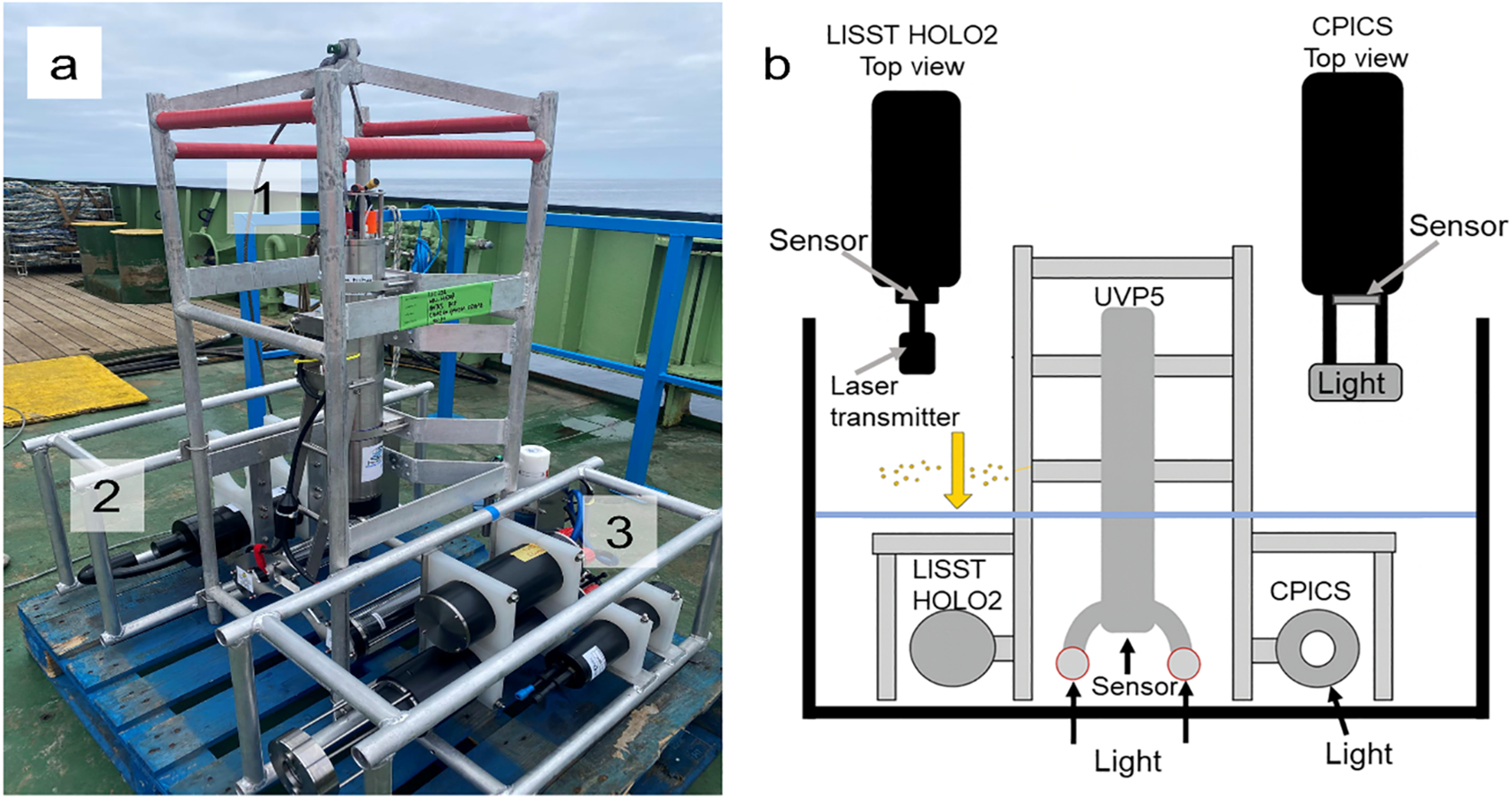
Images of assembled instruments and experiment setup. (a) Three optical devices mounted on a custom designed frame during the field works: UVP5 (1), LISST HOLO2 (2), and CPICS (3). (b) Schematic picture of experimental setup.
2.1 Underwater vision profiler 5
The UVP5 (Hydroptics, France) is an optical instrument developed for imaging large particles, such as aggregates and zooplankton, in aquatic environments (Picheral et al., 2010). The camera is mounted vertically, facing downward approximately 40 cm above the light source, capturing images along its path at a frequency of 20 Hz. The sampling volume spans 3.11cm in depth with a field of view of 22 cm × 18 cm. Illumination is provided by 42 red LEDs with a wavelength of 625 nm and flashes of approximately 100 µs duration, as described by the manufacturer. Images are recorded in grayscale with a pixel resolution of 88 µm. An internal processor (x86 AMD Geode GX533, 400 MHz CPU) in the camera housing automatically extracts in-focus particles, or regions of interest, to internal memory. Although the system has the option to save full-frame images, we opted to save only regions of interest to optimize memory use. The system also provides an algorithm that automatically generates size distributions; however, we applied our algorithm to generate size distributions for comparisons with other systems.
2.2 LISST HOLO2
The LISST HOLO2 (Sequoia Scientific, Inc., USA) records holographic images using optical interference and diffraction to provide three-dimensional views of particles. The electronic sensor (CCD) is positioned horizontally, approximately 50 mm from the laser housing, which emits collimated laser light with a wavelength of 658 nm. As particles pass through the laser’s optical path, they generate interference patterns that are captured as holograms. These holograms are recorded at a frequency of 10 Hz, with a pixel resolution of 4.4 µm, providing a field of view of approximately 5.3 mm × 7.0 mm and a sample volume of ~1.8 cm³ per hologram. The recorded holograms require digital reconstruction to produce actual images of the particles. We used the particle image extraction software suite FastScan, developed by the University of Aberdeen, for hologram reconstruction and auto-focusing (Liu et al., 2023; Thevar et al., 2023), which extracts in-focus particles as regions of interest.
2.3 Continuous plankton imaging and classification sensor
The CPICS (Coastal Ocean Vision, USA) records images in RGB color, capturing particles in true color. The camera (Prosilica GT 1380) is positioned horizontally, with white strobe lights mounted opposite the camera to provide uniform illumination. The sample volume is approximately 0.33 cm³, with a field of view measuring 1.5 cm × 1.1cm. Particles moving through the sampling volume are recorded at a frequency of 10 Hz, with a pixel resolution of 4.5 µm. An internal Jetson TX2 processor automatically detects in-focus particles, or regions of interest, and stores them in internal memory. Although full-frame savings are available, we opted to save only the regions of interest to optimize memory usage.
2.4 Calibration particles
Olive stone granules (BioPowder.com, https://www.bio-powder.com/en/) were used as reference particles with known size ranges due to their hydrophobic properties, which help to minimize light reflection and scattering during imaging with the optical instruments. Five distinct particle size ranges (0 - 50 µm, 100 - 300 µm, 300 - 600 µm, 600 - 800 µm, and 800 - 1000 µm) were defined to represent the overall span of particle sizes considered in this study. These ranges were merged into a continuous dataset for subsequent analysis of the full size spectrum for all the instruments, enabling validation of the size spectra across the instruments.
3 Methods
3.1 Calibration setup
Calibration experiments were conducted on two separate occasions (26 May 2022 and 22 April 2023) using a plastic container with dimensions of approximately 1.5 m × 1.5 m × 1 m (Figure 1b). The instrument frame, housing the three optical devices, was positioned vertically within the container to replicate its orientation during field operations. Fresh water at approximately 20 °C was used to prevent particle buoyancy or aggregation caused by salinity gradients. The water level was maintained at a consistent height of 0.5 m throughout both experiments to ensure stable conditions.
During the preliminary trials, particles were mixed with water in a small bottle and then released above the sampling volume of each instrument by gently squeezing the bottle. This method facilitated particle introduction but posed challenges in ensuring precisely controlling the volume of particles uniformly passing through the sampling volume of the instruments. Additionally, the process of squeezing the particle-water mixture out of the bottle caused excessive initial velocity to the particles, resulting in motion blur and reduced image quality. The method of particle introduction was refined to reduce particle velocity and minimize motion blur, enhancing image quality. Particles were gradually introduced using a small plastic container, held approximately 5cm from the water surface. We merged particles of five size classes (5 grams per particle size class) and released them from the container for approximately 30 seconds allowing them to become naturally moistened at the surface. Particles were then left to settle naturally through the sampling volume, minimizing turbulence and enhancing uniform distribution. Particle images were simultaneously captured by the three instruments throughout the experiments and a total of 391,828 images, 23,030 images, and 53,602 images were 244 recorded by UVP5, CPICS and LISST HOLO2, respectively.
3.2 Measuring particle sizes
Image filtering to separate particles and artefactual features (i.e. extreme motion blur, bubbles and interference patterns, Supplementary Figure S1) was performed by trained convolutional neural network (AlexNet, F-1 score = 0.9, detailed method in Supplementary Materials). Although 20 - 40% of images were excluded during filtering, most removals reflected optical artifacts or poorly resolved features rather than true particle absence. Including such detections would distort size spectra due to motion blur, focus errors, or scattering artifacts. We therefore retained only particles with reliably measurable morphology, following standard plankton imaging practice. All filtered images were then converted into grayscale and binarized to facilitate size analysis. We used the regionprops function in MATLAB (R2023b, Mathworks Inc.) to approximate each particle as an ellipse and extract geometric properties. Two metrics were used to characterize particle sizes; major axis length (MajAL, in cm) corresponding to the length of the major axis of the best-fit ellipse, and equivalent spherical diameter (ESD, in cm), calculated as the diameter of a two-dimensional circle with the same area as the detected particle region. For all instruments, a minimum particle size threshold of 5 pixels was set to ensure reliable particle recognition. Since each imaging system produces different types of images, we applied four binarizing algorithms to determine the most effective method to detect particles - Otsu, Canny, Sobel, and Prewitt. Each algorithm offers a distinct approach to separating particles from the background and identifying particle features and they are commonly compared when selecting robust edge detection method (Canny, 1986; Liu et al., 2018; Onyedinma Ebele et al., 2025; Otsu, 1979). We visually inspected the subset of binarized images based on three criteria: (1) edge clarity, the degree to which particle are clearly separating particles from the background, with continuous boundaries and minimal noise; (2) fragmentation, evaluating whether the full shape of each particle is retained without breakage; (3) completeness, assessing whether all visible particles are fully captured. To confirm that our simplified approach with a default setting provided robust results, a 10% subset of images was also processed with additional preprocessing (background correction, denoising, and contrast normalization) and with optimized Canny thresholds (the most parameter-sensitive method) following Ohman et al. (2019). Results differed by less than 10% from the defaults and the changes in particle outlines were negligible; the optimized thresholds and the number of edge pixels remained consistent. These checks confirm that the default settings provided robust and reproducible edge detection across instruments.
3.3 Size distribution
We constructed number size spectra using logarithmically increasing size bins (following Petrik et al., 2013), a powerful method to describe size distribution of marine particles, where large particles are typically less common. Number of particles, N, in each logarithmically increasing size bin (MajAL and ESD; 0.01 cm - 0.56 cm with 100.065 cm bin width) was calculated. Nlog was divided by the bin width and the sample volume (Vim) to obtain normalized particle abundance (n = N/(bin width)/Vim), and log10(n) was plotted against the logarithm of the average bin size to construct a number size spectrum. Any bin with the insufficient number of particles N < 10 was discarded before computing the spectrum. Normalized particle abundance - defined as (raw particle count divided by total sample volume and bin width, n, cm4) was plotted as a function of particle size. For each instrument, size spectra were plotted together, and raw particle counts in each bin were indicated in color (Figure 2), highlighting the most abundant size bin for each instrument. This comparison allowed us to confirm that the normalization procedure did not alter the relative shape of the size distributions. We also fitted linear regression lines from the peak of number.
Figure 2
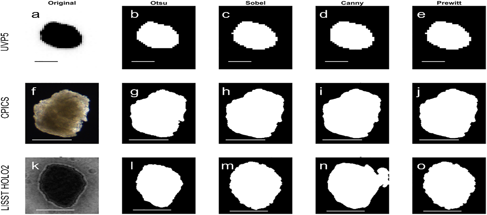
Example images of particles in uniform shapes showing the small difference in the different thresholding methods when images are clear. Columns show (a, f, k) original image, (b, g, l) Otsu, (c, h, m) Sobel, (d, i, n) Canny and (e, j, o) Prewitt. Upper row (a–e) UVP5: binarized images are almost identical. Middle row (f–g) CPICS: binarized images are almost identical. Bottom row (k–o) LISST HOLO2: particle was slightly overestimated by Canny.
4 Results and discussion
4.1 Impact of thresholding methods on binarization quality and particle sizes
For high particle-background contrast images, four thresholding methods (Otsu, Sobel, Canny and Prewitt) showed similar outcomes of binarized images (Figure 2) and passed our visual inspection criteria (edge clarity, fragmentation and completeness). In contrast, for images with irregular patterns, the method choice became more critical for the binarization quality (Figure 3), resulting in failing the visual inspection and inaccurate particle size measurements. For example, when UVP5 captured multiple particles within the regions of interest and there was a contrast between particles (with one darker than the other), Otsu thresholding failed to accurately capture the full shape of the lighter-colored particle (i.e. failing completeness) (Figure 3b). It incorrectly detected the dark spot within the light-colored particle and erased the lighter portion, leading to underestimation of particle abundance and sizes- up to 80% smaller when the particle-background contrast was weak (contrast ratio, minimum intensity/maximum intensity > 0.5). Similarly, Otsu thresholding was less effective when CPICS captured particles with highly reflective spots and weak contrast between the particle and background (i.e. failing edge clarity and fragmentation) (Figure 3g), resulting in underestimating particle size - up to 65% smaller when the contrast ratio exceeded 0.8. In both cases, Canny thresholding provided more accurate particle descriptions (Figures 4d, i). In contrast, Otsu thresholding accurately described particles for LISST HOLO2 even when the interference pattern around the particles was prominent (Figure 3k), while Canny thresholding tended to overestimate particle sizes in this instance - up to approximately four times larger - by detecting the noise around the particles (i.e. failing the edge clarity) (Figure 4n).
Figure 3
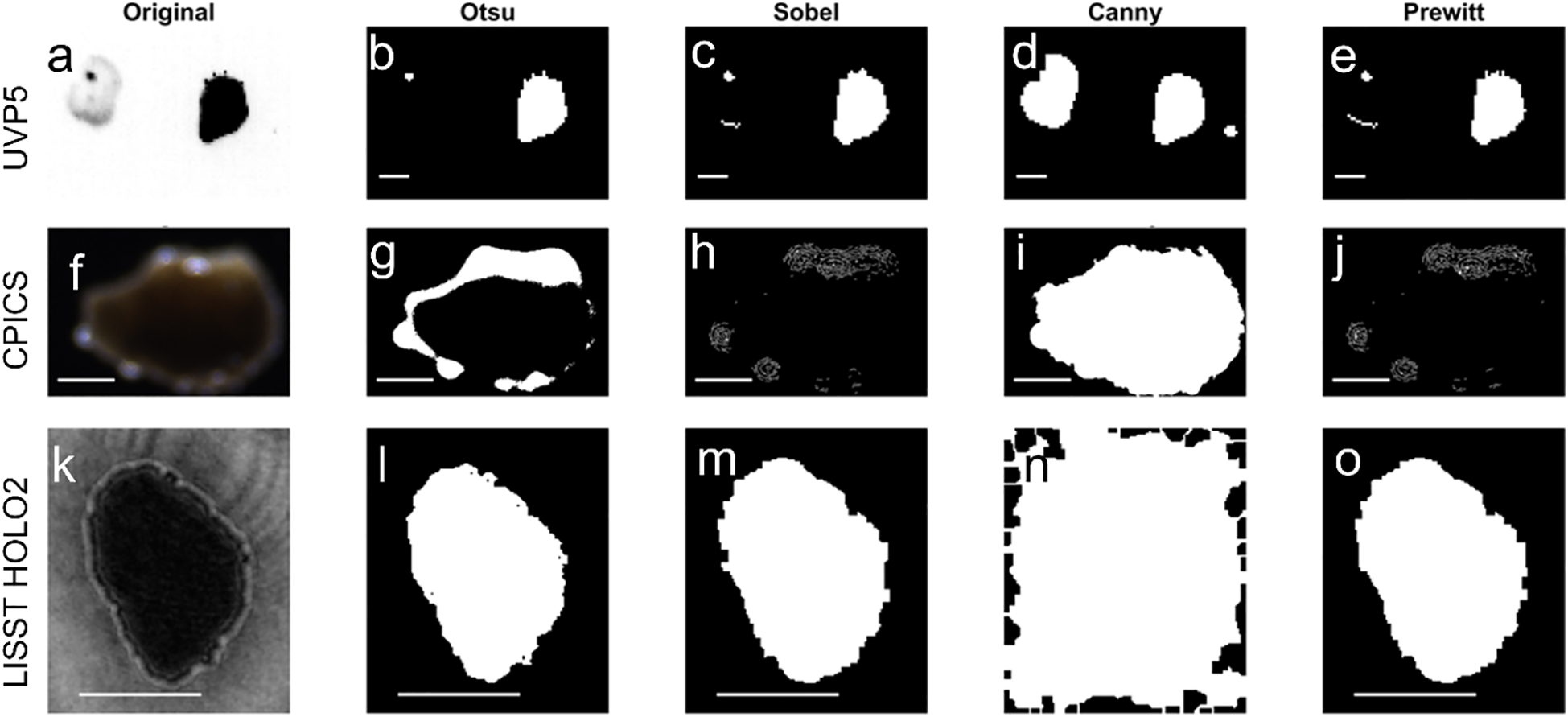
Example image of non-standard particles highlighting the need for careful selection of thresholding algorithms, which may have to differ for different instruments. Columns show (a, f, k) original image, (b, g, l) Otsu, (c, h, m) Sobel, (d, i, n) Canny and (e, j, o) Prewitt. Upper row (a–e) UVP5: Two particles with different lighting are best picked up by Canny. Middle row (f–g) CPICS: particles with high reflecting spots and weak contrast between particle and background are best described by Canny. Bottom row (k–o) LISST HOLO2: Particles with interference patterns in the background are best described b.
Figure 4
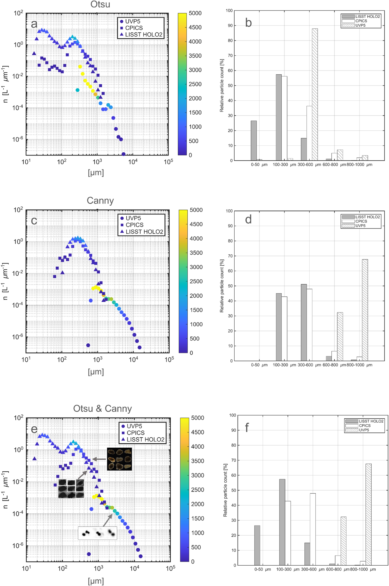
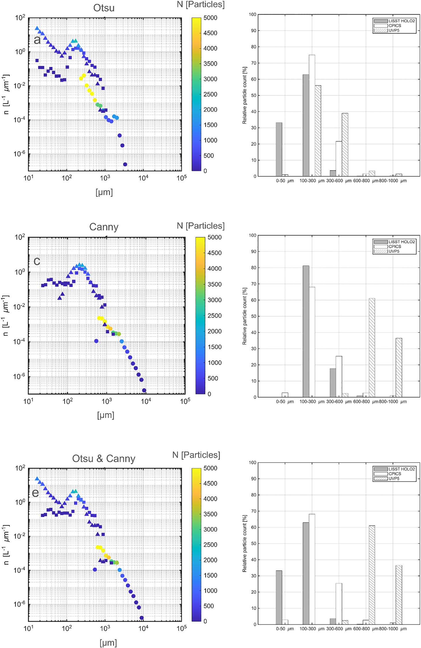
Particle size distributions in MajAL computed from different binarization methods. (a, b) Otsu thresholding; (c, d) Canny thresholding; (e, f) Otsu thresholding for LISST-HOLO2 and Canny thresholding for UVP5 and CPICS. Left panels (a, c, e) Number size spectra - Normalized particle abundance (n, L-1 μm-1) against sizes (MajAL, μm). Circles: UVP5; Squares: CPICS; Triangles: LISST HOLO2. Color indicates the raw particle counts of particles in each size bin. Right panels (b, d, f) Relative particle counts from each instrument (%) within the five distinct size ranges used in the experiments. White with diagonal lines: UVP5;Solid white: CPICS; Solid gray: LISST-HOLO2.
We further investigated how the different binarization methods impact on the number size spectra by comparing the spectra generated from the sizes measured using Otsu thresholding and Canny thresholding methods (Figures 4a-d-f). The underestimation of weakly contrasted particle sizes by CPICS and UVP5 under Otsu thresholding resulted in aparent high abundance of small particles (MajAL < 0.01 cm for and CPICS, MajAL < 0.1 cm for UVP5) (Figure 4a) which was not observed in the size spectra generated using the Canny thresholding method (Figure 4c). This trend is reflected in the fitted linear regression slopes from the peak of each size spectrum, which were steeper for Otsu (-3.44 for UVP5, -3.91 for CPICS, -5.86 for LISST HOLO2) than for Canny (-2.98, -4.30, and -5.63, respectively), indicating that Otsu detects proportionally fewer large particles. In contrast, Canny thresholding tends to overestimate the size of particles in LISST HOLO2 images when interference patterns remain visible around the particles (Figure 3n). This led to an apparent excess of larger particles (MajAL > 0.1 cm) and absence of small particles (MajAL < 0.01 cm) in the resulting size spectra (Figure 4c).
The influence of the thresholding algorithm on particle size measurements and consequently size spectra, as observed in our results, is particularly surprising given that we are using fairly homogeneous and ‘simple-shaped’ particles with clearly defined edges. This finding suggests the substantial impact of the thresholding method selection on particle size measurements and subsequent interpretations with in-situ biological particles, which typically possess more complex shapes and less defined edges (Giering et al., 2020b). Indeed, the limitations of edge detection, and resulting inaccurate measurements of particle size and abundance, have been reported for measurements of complex-shaped natural particles (i.e. filament, spines), which can have critical consequences when size estimates are converted to ecological parameters such as biovolume (Huang and Bochdansky, 2025; Kraft, 2021; Sosik and Olson, 2007). Although, we selected Canny for UVP5 and CPICS, and Otsu for LISST HOLO2 for the further analysis because these methods performed the most accurate edge detection, these earlier studies on natural particles highlight that routine visual inspection remains crucial to identify the most effective method and reduce misinterpretation in future in-situ work. One effective approach would be to generate a collage of images (raw + binarized, such as Figures 2, 3) for, at least, 5 randomly selected images within each size bin. This visual inspection will help researchers assess whether the chosen thresholding algorithm is appropriate to describe the particle size spectra. Such careful inspection and selection of suitable binarization methods will be even more crucial when measuring the natural particles, such as marine snow, as these exhibit more complex shapes and edges (Giering et al., 2020b; Liu et al., 2023) compared to the uniform particles with well-defined edges used in this study.
4.2 Size distribution: number size spectra
The observed particle size across the three instruments ranged from 100 µm to 1 cm, which exceeded the maximum size of the source particles (1 mm) used in the experiment. Visual inspection of the images revealed that these unexpected large particles were due to particle flocculation. Since flocculation is a natural process that can be seen in any aquatic system (e.g. marine snow), we did not exclude these large particles as noise. The size spectra for each instrument (Figures 4, 5) shows distinct peaks corresponding to the most frequently detected particle sizes. The highest raw counts of particles per bin were observed at 0.02 cm, 0.03 cm, 0.09 cm for LISST HOLO2, CPICS, and UVP5, respectively. These bins provide more statistically stable (i.e., less noisy) estimates of relative abundance because they contain more observations, although this does not necessarily imply greater sizing accuracy. While normalized particle numbers typically decrease continuously as bin sizes increase, fluctuations along the size spectra (peaks and troughs) can occur naturally [e.g. through cohorts or high abundance of a particular species (Zhou et al., 2009; Giering et al., 2019)] or because the bin size approached the limit of detection for a given instrument. The latter is often associated with a ‘dropping off’ in the slope towards the extremes of the instrument-specific spectra. Bins containing very few detected particles carry higher sampling uncertainty in their estimated concentrations and should therefore be interpreted with caution, particularly when combining spectra from different instruments. We suggest including the raw particle counts in the number size spectra (as indicated in color in Figures 4, 5) as a potential guideline to validate the reliability of the number size spectra. In our case, this examination method revealed that the UVP5 and LISST-HOLO2 size spectra align best when two different thresholding algorithms are used (Figure 4e).
Figure 5
Particle size distributions in ESD computed from different binarization methods. (a, b) Otsu thresholding; (c, d) Canny thresholding; (e, f) Otsu thresholding for LISST-HOLO2 and Canny thresholding for UVP5 and CPICS. Left panels (a, c, e) Number size spectra - Normalized particle abundance (n, L-1 μm-1) against sizes (ESD, μm). Circles: UVP5; Squares: CPICS; Triangles: LISST HOLO2. Color indicates the raw particle counts of particles in each size bin. Right panels (b, d, f) Relative particle counts from each instrument (%) within the five distinct size ranges used in the experiments. White with diagonal lines: UVP5; Solid white: CPICS; Solid gray: LISST-HOLO2.
To further evaluate the effective detection ranges of each instrument, we quantified their relative contributions to total particle counts across five defined size classes (Figures 4b, d, f). Under the Otsu thresholding, LISST-HOLO2 dominated detections in the small size classes (0 - 50 µm and 100 - 300 µm; 84%), whereas UVP5 accounted for nearly all detections in the largest ranges (> 300 µm; >98.6%). CPICS contributed primarily to the intermediate range (100 - 300 µm; 56%), reflecting its optimal detection window. Under the Canny thresholding, the overall pattern was similar: LISST-HOLO2 and CPICS detected the majority of particles below 600 µm (up to 96.1% and 90.7%, respectively), whereas UVP5 was dominant above 600 µm (up to 99.9%). These results confirm that each instrument performed best within its designed operational size range - LISST-HOLO2 for small particles, CPICS for intermediate sizes, and UVP5 for larger particles. Although both thresholding methods produced consistent overall trends, our comparison showed least misinterpretation of particle features during binarization (Figure 3), and the size spectra aligned most closely when the Otsu method is applied to the LISST-HOLO2 and the Canny method to the CPICS and UVP5 (Figure 4e). This indicates that applying the Otsu thresholding to LISST-HOLO2 and the Canny thresholding to CPICS and UVP5 provides the most effective approach in our setup.
We also constructed size spectra using ESD to evaluate how different size approximations influence the size spectra (Figure 5). Since particles are transformed into spherical shapes to obtain ESD, ESD naturally appears smaller than MajAL for elongated particles. The degree of difference between the two can vary with particle shape, and this sensitivity becomes important when analyzing marine particles that have large variations in the shape. While our number size spectra did not show significant differences between MajAL and ESD - likely because our particles were relatively uniform in shape - we observed a slightly higher abundance of small sizes with ESD. The choice between MajAL and ESD should therefore depend on the aim of analysis with natural marine particles. For example, ESD may be more useful when studying volume-based or mass-related processes, while MajAL may be more important when studying the dynamics of particles. In particular, turbulence can cause fragmentation, and the Kolmogorov scale (the smallest eddy scale) can be a key factor in fragmentation (Takeuchi et al., 2019).
Overall, the three number size spectra were well aligned despite variations in the recording system between the instruments (Figures 4e, 5e), demonstrating that multiple optical imaging systems can be effectively combined to generate a continuous size spectrum across broad size ranges. Comparable comprehensive size spectra have also been produced by combining sequentially collected in-situ plankton images (Jackson et al., 1997; Stemmann et al., 2008; Zhang et al., 2023; Dugenne et al., 2024; Lombard et al., 2019; Greer et al., 2020b). A key distinction of our study is that all instruments are mounted on the same frame capturing images simultaneously and ensuring consistent measurement conditions across instruments. Since environmental conditions can alter particle number size spectra, simultaneous deployment is crucial when using multiple instruments to construct a comprehensive size spectrum in dynamic systems. Time scale matters as if the interval between sequential deployments is longer than the time processes that alter size spectra, the resulting conclusions may be misleading. Turbulence, for example, can make change rapidly (on the order of seconds to minutes) and may also drive a significant change during extreme event such as storms. Such change in turbulence can influence the particle dynamics through dispersion and avoidance behavior of plankton (Haury et al., 1990; Incze et al., 2001) (Basterretxea et al., 2020; Durham, 2013) or aggregation and fragmentation of marine snow (Rühl and Möller, 2024). For the longer time scale (several hours to days), biological processes may have a pronounced influence on particle dynamics; such as growth of phytoplankton (Prairie, 2019), zooplankton grazing (Giering, 2014) or zooplankton diurnal vertical migration (Ohman and Romagnan, 2016). Our setup which allows deploying the entire system on a single frame is therefore an effective setup to minimize spatiotemporal variability and produce more directly comparable size spectra from each instrument. On a practical level, the operation of all instruments on one frame makes deployment easier and ensures that the sampling conditions, such as lowering speed and potential ship-based influences (i.e. waves and ship motions) - all of which can affect size spectra through e.g. disaggregation, avoidance and attraction of zooplankton - are the same.
5 Conclusion
This study demonstrated that integrating three optical imaging instruments on a single platform enables the computation of continuous particle size spectra spanning several orders of magnitude -from micrometers to centimeters. The experiment revealed that the selection of the binarization method is critical when examining particle size distributions. Although the particles used in this study were relatively uniform in shape, we found that some methods effectively captured particle boundaries and sizes, while others misrepresented particle shapes - depending on the image type. Such misinterpretation can substantially affect the derived size spectra and, consequently, the ecological interpretation of particle size distributions. Careful inspection and validation of binarization outcomes are therefore strongly recommended. While we adopted a simplified binarization workflow in this study, further parameter tuning may be necessary when analyzing more complex or irregularly shaped marine particles.
Our findings also highlight that the choice of size metric - equivalent spherical diameter (ESD) versus major axis length (MajAL) - strongly influences the resulting size spectra and its interpretation. By integrating multiple instruments and addressing these methodological aspects, we established a robust framework for constructing number size spectra across broad size ranges. Such measurements spanning broad particle size ranges are directly applicable to in situ observations and enhance our understanding of particle-driven carbon fluxes and ecosystem dynamics.
Statements
Data availability statement
The raw data supporting the conclusions of this article will be made available by the authors, without undue reservation.
Author contributions
MT: Conceptualization, Methodology, Validation, Visualization, Writing – original draft, Writing – review & editing, Data curation, Formal Analysis, Investigation, Software. ZL: Software, Writing – original draft, Writing – review & editing. WM: Investigation, Writing – original draft, Writing – review & editing. YVC-P: Investigation, Software, Writing – original draft, Writing – review & editing. TT: Software, Writing – original draft, Writing – review & editing. JW: Investigation, Writing – original draft, Writing – review & editing. SG: Conceptualization, Funding acquisition, Methodology, Project administration, Resources, Supervision, Validation, Visualization, Writing – original draft, Writing – review & editing.
Funding
The author(s) declare that financial support was received for the research and/or publication of this article. This work was supported through the ANTICS project, receiving funding from the European Research Council (ERC) under the European Union’s Horizon 2020 research and innovation programme (Grant Agreement No 950212). YVCP’s participation was supported through a shipboard training fellowship from Nippon Foundation and the Partnership for Observation of the Global Ocean.
Acknowledgments
We thank Kevin Saw, David Paxton and Stephen Shorter for helping with the logistics of the calibration experiments.
Conflict of interest
The authors declare that the research was conducted in the absence of any commercial or financial relationships that could be construed as a potential conflict of interest.
Generative AI statement
The author(s) declare that no Generative AI was used in the creation of this manuscript.
Any alternative text (alt text) provided alongside figures in this article has been generated by Frontiers with the support of artificial intelligence and reasonable efforts have been made to ensure accuracy, including review by the authors wherever possible. If you identify any issues, please contact us.
Publisher’s note
All claims expressed in this article are solely those of the authors and do not necessarily represent those of their affiliated organizations, or those of the publisher, the editors and the reviewers. Any product that may be evaluated in this article, or claim that may be made by its manufacturer, is not guaranteed or endorsed by the publisher.
Supplementary material
The Supplementary Material for this article can be found online at: https://www.frontiersin.org/articles/10.3389/fmars.2025.1538403/full#supplementary-material
References
1
Accardo A. Laxenaire R. Baudena A. Speich S. Kiko R. Stemmann L. (2025). Intense and localized export of selected marine snow types at eddy edges in the South Atlantic Ocean. Biogeosciences22, 1183–1201. doi: 10.5194/bg-22-1183-2025
2
Basterretxea G. Font-Muñoz J. S. Tuval I. (2020). Phytoplankton orientation in a turbulent ocean: A microscale perspective. Front. Mar. Sci.7. doi: 10.3389/fmars.2020.00185
3
Burd A. B. Jackson G. A. (2009). Particle aggregation. Ann. Rev. Mar. Sci.1, 65–90. doi: 10.1146/annurev.marine.010908.163904
4
Cael B. B. Cavan E. L. Britten G. L. (2021). Reconciling the size-dependence of marine particle sinking speed. Geophys Res. Lett.48, e2020GL091771. doi: 10.1029/2020GL091771
5
Canny J. (1986). A computational approach to edge detection. IEEE Trans. Pattern Anal. Mach. Intell.8, 679–698. doi: 10.1109/TPAMI.1986.4767851
6
Chisholm S. W. (1992). “ Phytoplankton size,” in Primary productivity and biogeochemical cycles in the sea. Eds. FalkowskiP. G.WoodheadA. D.ViviritoK. ( Springer US, Boston, MA), 213–237. doi: 10.1007/978-1-4899-0762-2_12
7
Clements D. J. (2022). Constraining the particle size distribution of large marine particles in the global ocean with in situ optical observations and supervised learning. Global Biogeochem Cycles36, e2021GB007276. doi: 10.1029/2021GB007276
8
Dugenne M. Corrales-Ugalde M. Luo J. Y. Kiko R. O’Brien T. D. Irisson J.-O. et al . (2024). First release of the Pelagic Size Structure database: global datasets of marine size spectra obtained from plankton imaging devices. Earth Syst. Sci. Data16, 2971–2999. doi: 10.5194/essd-16-2971-2024
9
Durham W. M. (2013). Turbulence drives microscale patches of motile phytoplankton. Nat. Commun.4, 2148. doi: 10.1038/ncomms3148
10
Giering S. L. (2014). Reconciliation of the carbon budget in the ocean's twilight zone. Nature507, 480–483. doi: 10.1038/nature13123
11
Giering S. L. C. Cavan E. L. Basedow S. L. Briggs N. Burd A. B. Darroch L. J. et al . (2020a). Sinking organic particles in the ocean—Flux estimates from in situ optical devices. Front. Mar. Sci.6. doi: 10.3389/fmars.2019.00834
12
Giering S. L. C. Hosking B. Briggs N. Iversen M. H. (2020b). The interpretation of particle size, shape, and carbon flux of marine particle images is strongly affected by the choice of particle detection algorithm. Front. Mar. Sci.7. doi: 10.3389/fmars.2020.00564
13
Giering S. L. C. S. L. C. Wells S. R. S. R. Mayers K. M. J. K. M. J. Schuster H. Cornwell L. Fileman E. S. E. S. et al . (2019). Seasonal variation of zooplankton community structure and trophic position in the Celtic Sea: A stable isotope and biovolume spectrum approach. Prog. Oceanogr177, 101943–101943. doi: 10.1016/j.pocean.2018.03.012
14
Greer A. T. (2020b). High-resolution sampling of a broad marine life size spectrum reveals differing size- and composition-based associations with physical oceanographic structure. Front. Mar. Sci.7. doi: 10.3389/fmars.2020.542701
15
Guidi L. (2009). Effects of phytoplankton community on production size and export of large.pdf. Limnology Oceanogr54, 1829–2272. doi: 10.4319/lo.2009.54.6.1951
16
Guidi L. Jackson G. A. Stemmann L. Miquel J. C. Picheral M. Gorsky G. (2008). Relationship between particle size distribution and flux in the mesopelagic zone. Deep Sea Res. Part1, 1364–1374. doi: 10.1016/j.dsr.2008.05.014
17
Haury L. R. Yamazaki H. Itsweire E. C. (1990). Effects of turbulent shear flow on zooplankton distribution. Deep Sea Res. Part1 37, 447–461. doi: 10.1016/0198-0149(90)90019-R
18
Huang H. Bochdansky A. B. (2025). Optimizing an image analysis protocol for ocean particles in focused shadowgraph imaging systems. Front. Mar. Sci.12. doi: 10.3389/fmars.2025.1539828
19
Incze L. S. Hebert D. Wolff N. Oakey M. Dye D. (2001). Changes in copepod distributions associated with increased turbulence from wind stress. Mar. Ecol. Prog. Ser.213, 229–240. doi: 10.3354/meps213229
20
Jackson G. A. (1990). A model of the formation of marine algal flocs by physical coagulation processes. Deep Sea Res. Part A. Oceanogr Res. Papers37, 1197–1211. doi: 10.1016/0198-0149(90)90038-W
21
Jackson G. A. Maffione R. Costello D. K. Alldredge A. L. Logan B. E. Dam H. G. (1997). Particle size spectra between 1 μm and 1 cm at Monterey Bay determined using multiple instruments. Deep Sea Res. Part Oceanogr Res. Pap44, 1739–1767. doi: 10.1016/S0967-0637(97)00029-0
22
Kraft K. (2021). First application of IFCB high-frequency imaging-in-flow cytometry to investigate bloom-forming filamentous cyanobacteria in the baltic sea. Front. Mar. Sci.8. doi: 10.3389/fmars.2021.594144
23
Liu Z. Giering S. Thevar T. Burns N. Ockwell M. Watson J. (2023). “ Machine-learning-based size estimation of marine particles in holograms recorded by a submersible digital holographic camera,” in OCEANS 2023 - ( Limerick Ireland: IEEE). 1–8. doi: 10.1109/OCEANSLimerick52467.2023.10244456
24
Liu Z. Watson J. Allen A. (2018). Efficient image preprocessing of digital holograms of marine plankton. IEEE J. Ocean Eng.43, 83–92. doi: 10.1109/JOE.2017.2690537
25
Lombard F. Boss E. Waite A. M. Vogt M. Uitz J. Stemmann L. et al . (2019). Globally consistent quantitative observations of planktonic ecosystems. Front. Mar. Sci.6. doi: 10.3389/fmars.2019.00196
26
Ohman M. D. Romagnan J. -B. (2016). Nonlinear effects of body size and optical attenuation on Diel Vertical Migration by zooplankton. Limnol. Oceanogr.61, 765–770. doi: 10.1002/lno.10251
27
Ohman M. D. Davis R. E. Sherman J. T. Grindley K. R. Whitmore B. M. Nickels C. F. et al . (2019). Zooglider: An autonomous vehicle for optical and acoustic sensing of zooplankton. Limnol Oceanogr Methods17, 69–86. doi: 10.1002/lom3.10301
28
Omand M. M. Govindarajan R. He J. Mahadevan A. (2020). Sinking flux of particulate organic matter in the oceans: Sensitivity to particle characteristics. Sci. Rep.10, 5582. doi: 10.1038/s41598-020-60424-5
29
Onyedinma Ebele G. Asogwa Doris C. Onwumbiko Joy N. (2025). Exploring the effectiveness of sobel, canny, and prewitt edge detection algorithms on digital images. World J. Adv Eng. Technol. Sci.15, 1722–1730. doi: 10.30574/wjaets.2025.15.1.0346
30
Otsu N. (1979). A threshold selection method from gray-level histograms. IEEE Trans. Syst Man Cybernetics9, 62–66. doi: 10.1109/TSMC.1979.4310076
31
Petrik C. M. Jackson G. A. Checkley D. M. (2013). Aggregates and their distributions determined from LOPC observations made using an autonomous profiling float. Deep Sea Res. Part Oceanogr Res. Pap74, 64–81. doi: 10.1016/j.dsr.2012.12.009
32
Picheral M. Guidi L. Stemmann L. Karl D. M. Iddaoud G. Gorsky G. (2010). The Underwater Vision Profiler 5: An advanced instrument for high spatial resolution studies of particle size spectra and zooplankton. Limnology Oceanogr: Methods8, 462–473. doi: 10.4319/lom.2010.8.462
33
Prairie J. C. Montgomery Q. W. Proctor K. W. Ghiorso K. S. (2019). Effects of Phytoplankton Growth Phase on Settling Properties of Marine Aggregates. J. Mar. Sci. Eng.7, 265. doi: 10.3390/jmse7080265
34
Reynolds R. A. Stramski D. Wright V. M. Woźniak S. B. (2010). Measurements and characterization of particle size distributions in coastal waters. J. Geophys Res.115. doi: 10.1029/2009JC005930
35
Rühl S. Möller K. O. (2024). Storm events alter marine snow fluxes in stratified marine environments. Estuarine Coast. Shelf Sci.302, 108767. doi: 10.1016/j.ecss.2024.108767
36
Sheldon R. W. Prakash A. Sutcliffe W. H. (1972). The size distribution of particles in the ocean1. Limnol Oceanogr17, 327–340. doi: 10.4319/lo.1972.17.3.0327
37
Simon M. Grossart H. P. Schweitzer B. Ploug H. (2002). Microbial ecology of organic aggregates in aquatic ecosystems. Aquat. Microbial Ecol.28, 175–211. doi: 10.3354/ame028175
38
Sosik H. M. Olson R. J. (2007). Automated taxonomic classification of phytoplankton sampled with imaging-in-flow cytometry. Limnology Oceanogr: Methods5, 204–216. doi: 10.4319/lom.2007.5.204
39
Stemmann L. Eloire D. Sciandra A. Jackson G. A. Guidi L. Picheral M. et al . (2008). Volume distribution for particles between 3.5 to 2000 μm in the upper 200 m region of the South Pacific Gyre. Biogeosciences5, 299–310. doi: 10.5194/bg-5-299-2008
40
Takeuchi M. Doubell M. J. Jackson G. A. Yukawa M. Sagara Y. Yamazaki H. (2019). Turbulence mediates marine aggregate formation and destruction in the upper ocean. Sci. Rep.9, 16280. doi: 10.1038/s41598-019-52470-5
41
Takeuchi M. Giering S. L. C. Yamazaki H. (2024). Size distribution of aggregates across different aquatic systems around Japan shows that stronger aggregates are formed under turbulence. Limnol Oceanogr69, 2580–2595. doi: 10.1002/lno.12686
42
Thevar T. Burns N. Ockwell M. Watson J. (2023). An ultracompact underwater pulsed digital holographic camera with rapid particle image extraction suite. IEEE J. Ocean Eng.48, 566–576. doi: 10.1109/JOE.2022.3220880
43
Williams J. R. Giering S. L. C. (2022). In situ particle measurements deemphasize the role of size in governing the sinking velocity of marine particles. Geophys. Res. Lett.49, e2022GL099563. doi: 10.1029/2022GL099563
44
Zhang X. Huot Y. Gray D. Sosik H. M. Siegel D. Hu L. et al . (2023). Particle size distribution at Ocean Station Papa from nanometers to millimeters constrained with intercomparison of seven methods. Elem. Sci. Anthr11, 94. doi: 10.1525/elementa.2022.00094
45
Zhou M. Tande K. S. Zhu Y. Basedow S. (2009). Productivity, trophic levels and size spectra of zooplankton in northern Norwegian shelf regions. Deep Sea Res. Part II Top. Stud. Oceanogr56, 1934–1944. doi: 10.1016/j.dsr2.2008.11.018
Summary
Keywords
optical instruments, marine snow, size distribution, calibration methods, thresholding
Citation
Takeuchi M, Liu Z, Major W, Contreras-Pacheco YV, Thevar T, Williams JR and Giering SLC (2025) Cross-calibration of multiple optical instruments for the measurement of particle size distributions in water. Front. Mar. Sci. 12:1538403. doi: 10.3389/fmars.2025.1538403
Received
02 December 2024
Revised
10 November 2025
Accepted
12 November 2025
Published
10 December 2025
Volume
12 - 2025
Edited by
David Alberto Salas de León, National Autonomous University of Mexico, Mexico
Reviewed by
Heidi M Sosik, Woods Hole Oceanographic Institution, United States
Kaisa Kraft, Finnish Environment Institute (SYKE), Finland
Updates
Copyright
© 2025 Takeuchi, Liu, Major, Contreras-Pacheco, Thevar, Williams and Giering.
This is an open-access article distributed under the terms of the Creative Commons Attribution License (CC BY). The use, distribution or reproduction in other forums is permitted, provided the original author(s) and the copyright owner(s) are credited and that the original publication in this journal is cited, in accordance with accepted academic practice. No use, distribution or reproduction is permitted which does not comply with these terms.
*Correspondence: Marika Takeuchi, Marika.Takeuchi@noc.ac.uk
Disclaimer
All claims expressed in this article are solely those of the authors and do not necessarily represent those of their affiliated organizations, or those of the publisher, the editors and the reviewers. Any product that may be evaluated in this article or claim that may be made by its manufacturer is not guaranteed or endorsed by the publisher.