 Huanqing Huang
 Alexander B. Bochdansky
- Department of Ocean and Earth Sciences, Old Dominion University, Norfolk, VA, United States
A variety of imaging systems are in use in oceanographic surveys, and the opto-mechanical configurations have become highly sophisticated. However, much less consideration has been given to the accurate reconstruction of imaging data. To improve reconstruction of particles captured by Focused Shadowgraph Imaging (FoSI)—a system that excels at visualizing low-optical-density objects, we developed a novel object detection algorithm to process images with a resolution of ~ 12 μm per pixel. Suggested improvements to conventional edge-detection methods are relatively simple and time-efficient, and more accurately render the sizes and shapes of small particles ranging from 24 to 500 μm. In addition, we introduce a gradient of neutral density filters as a part of the protocol serving to calibrate recorded gray levels and thus determine the absolute values of detection thresholds. Set to intermediate detection threshold levels, particle numbers were highly correlated with beam attenuation (cp) measured independently. The utility of our method was underscored by its ability to remove imperfections (dirt, scratches and uneven illumination), and by capturing the transparent particle features such as found in gelatinous plankton, marine snow and a portion of the oceanic gel phase.
1 Introduction
Investigating the spatiotemporal distribution of particulate organic matter and plankton organisms is essential for enhancing our understanding of the ocean ecology and particle fluxes. Over the years, methodologies used for collecting particle data have evolved from traditional tools such as plankton nets and sediment traps to cutting-edge optical systems including satellites and in-situ cameras. Optical instruments tailored for oceanographic observations, in terms of shadowgraph cameras including but not limited to In-situ Ichthyoplankton Imaging System (IRIIS), Zooplankton Visualization and Imaging System (ZooVIS) and other devices such as the Video Plankton Recorder (VPR), Underwater Vision Profiler (UVP), Lightframe On-sight Key species Investigation (LOKI), Zooglider, Laser In Situ Scattering, Transmissometry and Holography (LISST-Holo) and digital holographic cameras have expanded our insight into ocean particle abundances with their high spatiotemporal coverage (Davis et al., 1992; Gorsky et al., 1992; Cowen and Guigand, 2008; Picheral et al., 2010; Stemmann and Boss, 2012; Bochdansky et al. (2013); Schmid et al., 2016; Choi et al., 2018; Ohman et al., 2019; Giering et al., 2020a; Picheral et al., 2022; Daniels et al., 2023; Takatsuka et al., 2024; Li et al., 2024; Greer et al., 2025). However, given the variety of platforms there has not been a consensus on what constitutes a particle, and what does not, a problem that is exacerbated by the numerical dominance of particles with low optical density (OD) and reflectance (Bochdansky et al., 2022). As a result, a large portion – if not the majority – of aquatic particles have not been accounted for by the optical systems listed above due to the particle-gel continuum (Verdugo et al., 2004; Mari et al., 2017; Bochdansky et al., 2022). In other words, the number of particles per volume is largely dependent on the sensitivity of the instrument, and the threshold settings used in the binarization step from the original grayscale image (Bochdansky et al., 2022). Particle concentrations can therefore only be compared among deployments of the same optical system and identical calibration (e.g., Picheral et al., 2010) and when different instruments are compared the offsets in particle numbers have to be aligned among instrument platforms (Jackson and Checkley, 2011; Zhang et al., 2023).
Prior research has suggested that the choice of analytical methods for processing in-situ image data significantly influences the derived particle information (Schmid et al., 2016; Giering et al., 2020b), which implies a well-designed image analysis protocol can extract more useful information, while a poorly constructed one may hinder the visualization of potential patterns within the same dataset. A variety of particle detection methods have been employed in plankton image analysis, including global binarization (Sieracki, 1998; Davis et al., 2005), Canny Edge detection (Ohman et al., 2019; Orenstein et al., 2020), unsupervised learning segmentation (Cowen and Guigand, 2008; Iyer, 2012; Luo et al., 2018; Cheng et al., 2020b; Durkin et al., 2021; Takatsuka et al., 2024), and other image processing pipelines (Olson and Sosik, 2007; Tsechpenakis et al., 2007; Cheng et al., 2020a; Picheral et al., 2022). However, the literature provides limited detail on these methods. Additionally, the threshold, a primary parameter determining the number and size of particles in the processing algorithm, has often been set arbitrarily. For example, in the Focused Shadowgraph Imaging (FoSI) approach used in this study, which depends largely on light absorbance and to a much lesser extent on scatter, a higher threshold (indicating lower sensitivity) tends to reveal optically dense particles only, whereas lower thresholds with higher sensitivity enable us the visualization of additional particles with low OD (Bochdansky et al., 2022).
Moreover, to study small and low-optical-density particles via FoSI, acquiring particle information from images is complicated by the fact that particles ranging from tens to hundreds of micrometers are often represented by only a few pixels. Global thresholding implemented based on the gray level of image pixels, can produce noisy and incomplete particle edges when dealing with faint particles, which has a larger effect on the reconstruction of smaller particles biasing particle number spectra. While Canny edge detection reduces noise in images, it tends to overestimate edges and overlook smaller particles (Ma et al., 2017; Stephens et al., 2019; Giering et al., 2020b). Misinterpretation of large particles using unsuitable algorithms, especially for those consisting of multiple small fragments, further distorts the particle number spectrum (Bochdansky et al., 2022).
Even with the application of a currently elusive, ideal algorithm in terms of extracting particle images, the challenge increases when attempting to compare data across different optical systems. As a result, these cross-comparisons are exceedingly rare. Establishing robust and standardized criteria is thus crucial for creating objective benchmarks for particle detection. To address this issue, we propose the use of stepped neutral density (ND) filters containing 11 gradients with OD values from 0.04 to 1.0 as a calibration procedure for FoSI. While ND filters have not been widely used in oceanography as a standard reference, OD has been employed in ZooScan to ensure image comparability across various laboratory settings (Gorsky et al., 2010). In photomicrography, one study used ND filters as reference slides to obtain consistent images (Kim et al., 2011).
Here, we first describe an image processing protocol (Figure 1) tailored to the FoSI camera with neutral density filter calibration, preprocessing and quality enhancing algorithms, and the removal of images containing schlieren artifacts using machine learning. Implementing particle reconstructions at various sensitivity settings, we demonstrate the effect thresholds have on particle analysis. While our analysis is mostly geared towards shadowgraph imaging such as FoSI, ISIIS and ZooVIS, much of the image analysis tools provided here can be applied to other platforms as well. The narrative provides much detail and justifications for each individual step in the image analysis pipeline so that it simultaneously serves as an introduction and tutorial for novice users.
Figure 1. Pipeline of the image analysis protocol for image preprocessing, including illumination correction, image subtraction, and MicroDetect edge detection, followed by segmentation into small regions of interests (ROIs).
2 Materials and equipment
FoSI features a straightforward design with an inline configuration of illumination and camera resulting in high sensitivity and a large depth of field compared to non-shadowgraph imaging systems (Figure 2). A red-light LED (625 nm, Cree XLamp) is used as a point source. The light is collimated by a 25.4 mm plano-convex lens (focal length = 150 mm) and travels through 24.4 mm thick sapphire windows that delimit a sample space of exactly 3 cm before it is focused by another plano-convex lens (focal length = 100 mm) into a 25 mm camera lens (Marshall Electronic, V-4325, f/2.5) attached to a board camera (ImagingSource, model DMM 27UR0135-ML, 1/3” sensor). While only the center of the image volume is perfectly in focus, image blur is tolerable at extreme distances of the image volume and the blur is symmetrical so that the edges of particles are rendered accurately after binarization (Watanabe and Nayar, 1998; de Lange et al., 2024). The images are labeled consecutively with the date and time in the format {Image number} + {YY-MM-DD} + {HH-MM-SS}. Sorting the image sequence in chronological order from the beginning to the end is a crucial prerequisite for analysis in MATLAB, as the implemented function dir in the current analysis does not sort the list of data by their labeled image numbers. The captured images are in grayscale and saved as bitmaps. We do not recommend using jpeg or other compressions as we found artefacts associated with these formats after binarization (unpublished results).
Figure 2. Optical configuration of Focused Shadowgraph Imaging (FoSI). Built into a pressure case, the operational depth of this system is 6000 m. Dotted lines represent the light path. Rays are parallel across the imaging gap producing shadows on the sensor.
FoSI acquires 1280 960 pixels images, with a spatial resolution of 11.9 μm per pixel. The depth of field is adjustable depending on the oceanic system FoSI is deployed in. For the data presented in this study it was set to 3 cm, which lead to the total sample volume of ~5.18 milliliters per image before image subtraction. During image analysis, the image data were converted using function im2double() and analyzed as matrices of double-precision arrays rather than image variable (uint8 variable) because they allow the numbers to have decimals in their precision and are not limited to integers and the fixed numeric boundaries of 0 to 255. For instance, during the calculation of reference images, the rolling average of 100 sequential frames using uint8 variables cannot exceed 255, e.g., 100 + 200 equals to 300 numerically but in uint8, it is capped at 255. In other words, any pixel values greater than 255 are truncated to 255, and those less than 0 are set to 0.
Prior to image segmentation, the grayscale images were converted into binary images. A binary image contains only white (value = 1) and black (value = 0) pixels. The regions of interest (ROIs), which contain useful features, are represented by clusters of white pixels, while the black pixels form the background. The corresponding code for algorithms mentioned in the current study was created and executed using MATLAB 2022a (The MathWorks, Inc.).
Large batch analysis was conducted at Old Dominion University High Performance Computing Center (ODU HPC) run by bash scripts. We also compared beam attenuation, derived from light transmission data collected by a transmissometer (WET Labs C-Star, with a path length of 25 centimeters) and fluorescence (Chelsea Aqua 3) with the results analyzed by the current protocol, as well as UVP5 particle spectrum data from the same region and season but in a different year (Kiko et al., 2022).
3 Method
3.1 Illumination correction
Illumination unevenness impairs the accuracy of particle information, as varying brightness levels alter the dynamic range of pixels at different regions within the same image. Thresholding is a technique in image processing that converts grayscale images into binary images (black or white pixels). Local adaptive thresholding can overcome illumination unevenness since unlike global thresholding which applies a single threshold value to process the entire image, local adaptive thresholding determines the threshold value of a pixel by the small local neighborhood of that pixel (Otsu, 1975; Lie, 1995; Bradley and Roth, 2007; Singh et al., 2012; Roy et al., 2014). However, for consistency we employed global thresholding by using one constant threshold value across the entire image. Because of that, whole-image illumination correction was necessary. Based upon our investigation, flat-field correction, a method that removes the effects of illumination unevenness by applying an inverse matrix containing pixelwise correction factors of the uncorrected image and ideal even-illuminated image, has been used to effectively address this problem (Figure 3) (Seibert et al., 1998; Emerson and Little, 1999; Abdelsalam and Kim, 2011; Luo et al., 2018; Ohman et al., 2019; Wang et al., 2019). More precisely, flat-field correction involved creating a pixel-by-pixel correction factor matrix based on a standard gray level and a reference (or standard) image. This matrix was then applied to the original image to correct for variations in illumination, resulting in a more uniform final image (Figure 3). The binary image produced by global thresholding significantly benefited from prior illumination correction, as it served to alleviate the impact of edge effects and other uneven lighting issues. The current protocol adopted a correction method based on Wilkinson (1994). To implement this method, we first computed the correction factor for each pixel as described in Equation 1:
where Gain(x,y) denotes a matrix of a pixel-by-pixel correction factor, Gs the standard gray level, B(x,y) the blank image. While matrices are not capable of performing division operations with other matrices, Gs is assigned to each element in matrix B(x,y). The multiplication of correction factor matrix with the uncorrected image generates the corrected images,
where I(x, y) is the raw image, Gain(x, y) the output from Equation 2, and C(x, y) the corrected image.
Figure 3. Gradient neutral density filter before (left) and after (right) illumination correction. The darker stripes exhibit higher OD values than the lighter stripes in this original image positive.
Image correction begins with a standard gray level, a blank image, and a raw image (the image to be corrected). The standard gray level was determined by calculating the average gray level across the entire dataset (e.g., images of an entire cast), and this value was used as a reference for the correction process. The standard value was computed by first averaging the whole image sequence to one single image and then applying it to each pixel that is representative for the background gray level. Thus, the Gain function Equation 1 contains the correction factors for each pixel. A blank image is generated by averaging the deep-sea images with low particle concentration or images taken in particle free water (e.g., deionized water). Note that Equations 1, 2 should be applied to each image in the sequence after quality control and the obtained correction matrices might vary from image to image.
Overcorrection due to severely uneven illumination may occur when the images exhibit dark corner, in which case we capped the correction factors using clip() function to prevent this drawback. However, this step was not needed for images in this study and that exhibit minimal variance in illumination.
3.2 Image subtraction
Some severe artifacts such as dirt or scratches on optical surfaces may persist despite illumination correction, and image subtraction was subsequently applied to mitigate those artifacts. Function imabsdiff() is used to attain the subtraction (Equation 3),
where denotes the ith corrected image (numbered as ith image) in a chronological sequence, is in the second subtraction, in which j=i+1. denotes the subtraction results of two corrected images. The subtracted image can either be a blank image, or in oceanographic casts, two consecutive images are subtracted from each other. Each image is solely used once to avoid data redundancy (Figure 4), reducing the image number to half and increasing the image volume for the resultant images by twofold (to ~ 10 ml). It is noteworthy that a particle is only registered as a particle when it appears or disappears in sequential images. Particles that remain stationary, or those that are shaded by another particle in subsequent images are not registered. In typical oceanographic deployments, where water always moves in front of the camera, is typically replaced completely for each image, and when particle concentrations are low, shading and self-shading of particles represent a minor problem. In highly productive environments, with a significant amount shading, a blank image based on particle free water is a better choice.
Figure 4. A diagram of the illumination correction and subtraction. The illumination correction is implemented on each image, while the subtraction half the number of images.
3.3 Threshold calibration (gray level calibration)
The term “threshold” represents the gray level used to differentiate between the background and objects within an image during binarization. It is simply the sensitivity level at the post-production level (i.e., after the images were recorded), with a lower threshold corresponding to a higher sensitivity level.
To ensure the equivalency of sensitivity levels across different camera setups, a stepped ND filter (Edmund Optics, #32-599) was introduced for calibration purposes (Figure 5). The ND filter used in this study comprises 11 stripes, with OD ranging from 0.04 to 1.0, where lower OD values indicate more transparent stripes. OD, or absorbance in turn, is defined as
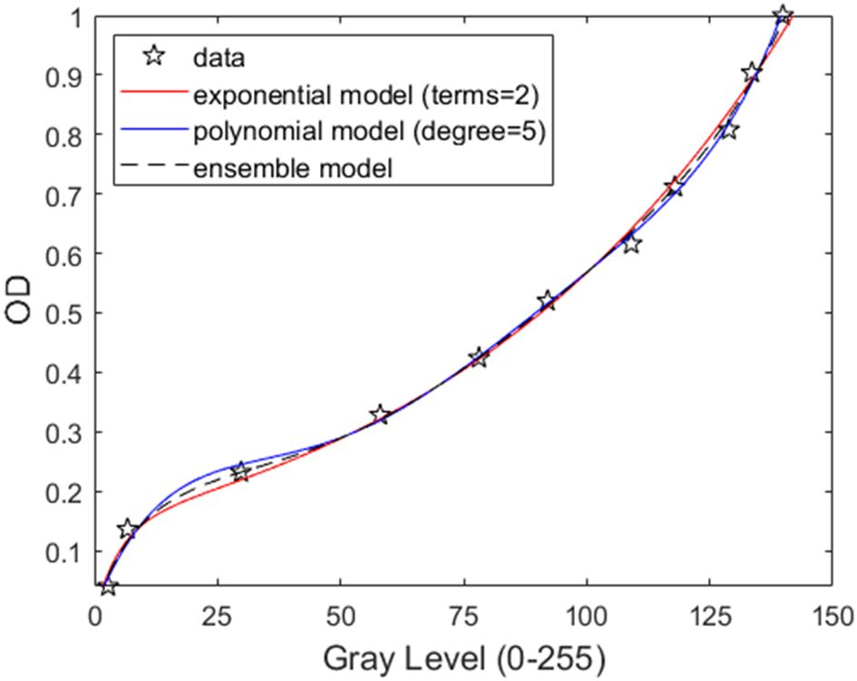
Figure 5. OD levels of the neutral density array plotted against their gray levels. The blue line represents a 5th order polynomial, the red line the 2-parameter exponential model, and the dashed black line the ensemble model.
where T is transmittance in % (Beer, 1852). According to Equation 4, an OD of 1 thus corresponds to a transmission of 10% of the light (90% absorbed).
The same illumination correction and subtraction procedures outlined in Section 3.1 and 3.2 were performed prior to measuring gray levels. A manually cropped 200 200 pixels area was subsequently selected, and the median gray level was computed for the corresponding OD strip. To predict the relationship between OD and gray level, the first model tested was a fifth-degree polynomial function (Equation 5), exhibiting an r2 value of 0.9992 (Figure 5).
where x here denotes gray level in this case. f(x) denotes the predicted OD value. p1, p2, p3, p4, p5, p6 denote the constants.
The exponential model also accurately predicted the relationship (Equation 6),
where x is the gray level and denotes the predicted OD. e denotes the exponential constant. a, b, c, d are the constant variables. Although the fit is slightly weaker than the previous one (r² = 0.9976), the prediction remains closely aligned with the observed OD for gray levels below 100.
Within the gray level interval between 0 and 50, the exponential model undershoots while the polynomial model overshoots the predicted OD value. Therefore, to achieve the highest accuracy, an ensemble model was used as shown in Equation 7,
where and are weighting factors for and , respectively. The dashed line in Figure 5 showed an example of choosing both weighting factors to be 0.5, which averages the results of the two models. The results of the ensemble model for corresponding OD values across gray levels 0 to 255 are provided in Supplementary Table 1.
3.4 The MicroDetect algorithm
This section is a critical component of our pipeline and named for the fact that detection of particles in the size range from 24 to 500 μm was optimized with this method. The name was derived from the Sieburth scale (Sieburth et al., 1978), which categorizes plankton into seven size classes. Here we show the major steps and underlying rationale for each step. Note this threshold-Canny combined algorithm was inspired by Nayak et al. (2015). The full MATLAB code together with example images is available in the Supplementary Section. Consult the MATLAB Imaging Toolbox for more details on the individual functions.
The first step involved a preprocessed grayscale image diff and a selected threshold value T (see below for the practical selection of threshold values) as the inputs of MicroDetect. A modified Canny edge detection function subsequently enhances the reconstruction of particles, for the purpose of noise reduction, and particle edges refinement. The edge detection was performed first through global thresholding, the command used here is Img=diff > T, where the pixels with gray level higher than T are classified as object pixels thus becoming white pixels in a binary image. Note “>“ was used since the image subtraction step results in image negatives with dark background and bright particles. Herein, the left side of the command was assigned as the names of the output image.
Following global thresholding, a simple morphological operation bridges 0-valued pixels with two or more 1-valued pixels in the neighborhood by Img1=bwmorph(Img, ‘bridge’). The neighborhood defined here refers to 8-connected pixels centering at the 0-valued pixels. The term 8-connectedness relates to how pixels touch each other. In 4-connectedness, pixels are only considered part of an edge when they touch on their flat sides. In 8-connectedness, they are considered a part of an edge if they touch on the corners as well. Next, an operation Img2=imfill(Img1, ‘holes’) function serves to fill the 0-valued pixels surrounded by 1-valued pixels. Particles less than 3 pixels were removed using Img3=bwareaopen(Img2, 3) to reduce noise.
Before applying Canny edge detection, we used the imclose function with Img4 = imclose(Img3, SE). This close operation performs a dilation followed by an erosion. Dilation expands the particles by adding more pixels to the boundaries, while erosion contracts them by removing pixels from the boundaries. This step further bridged the gaps of those nearby but unconnected clusters around the particle boundaries. The variable SE represents the structuring element, defined as SE = strel(‘disk’, 1). The structuring element is a matrix that determines whether a pixel is added or removed from a boundary by defining the shape of the neighborhood of that pixel (a disk-shaped structuring element in this case). Although the structuring element could be adjusted dynamically, the protocol only used a single value for consistency.
Conventional Canny edge detection involves four stages. All steps are integrated into one function named CannyDetection, which are called with the command Img5 = CannyDetection(Img4). This function operates in four steps as follows (Canny, 1986):
3.4.1 Smoothing
The input image is blurred with a 5x5 Gaussian filter (σ = 1.42).
3.4.2 Computing edge gradients
Sobel kernel filters illustrated in Figure 6 (Sobel and Feldman, 1968), were applied convolutionally to calculate the pixel intensity changes, also known as intensity gradients in horizontal (Gx) and vertical (Gy) directions respectively. The gradient magnitude for a given pixel G(x,y) was then computed by Equation 8:
![Two 3×3 operators labeled Gx and Gy. Gx contains values: top row [−1, 0, 1], middle row [−2, 0, 2], bottom row [−1, 0, 1]. Gy contains values: top row [1, 2, 1], middle row [0, 0, 0], bottom row [−1, −2, −1].](https://www.frontiersin.org/files/Articles/1539828/fmars-12-1539828-HTML-r1/image_m/fmars-12-1539828-g006.jpg)
Figure 6. The operators of Sobel edge detection. Gx and Gy calculate the intensity gradient in the x and y axis direction, respectively.
Since edge gradient is a vector defined by a quantity along with direction, the gradient directions, which represent the directions of the intensity gradients on the basis of the horizontal and vertical gradients, Gx and Gy, were determined using the four-quadrant inverse tangent function atan2(Gy, Gx), as given by Equation 9:
Subsequently, the directions were converted from radians to degrees and adjusted to 0°, 45°, 90°, or 135° with approximation. The identification of gradient directions facilitated the following non-maximum suppression step.
3.4.3 Non-maximum suppression
This step preserved only the maximum gradient in . The algorithm examined whether the processed pixel has the maximum gradient intensity in comparison to the adjacent two pixels along the gradient direction. The processed pixel preserved its gradient if it has the maximum gradient intensity, otherwise its gradient intensity is set to zero.
3.4.4 Hysteresis thresholding
Hysteresis thresholding allows the closely located line sections with only small gaps in between to form a continuous line. We set the lower and upper thresholds to be 0.01 and 0.02 of the maximum gradient intensity, respectively. The selection of lower and upper thresholds in Canny edge detection typically follows a ratio between 1:2 and 1:3. The ratio of these thresholds has a more significant influence on the results than using the specific threshold values. Additionally, empirical testing across various threshold ratios revealed minimal impact on the results when the ratio is equal to or less than 1:2. Specifically, pixels were classified based on their intensity gradient: those with gradients higher than the upper threshold were marked as edge pixels, whereas those below the lower threshold were marked as non-edges, and those with gradients in between were considered edge pixels only if they connected to pixels above the upper threshold.
A series of delicate morphological operations were performed after Canny edge detection. The function Img6=bwmorph(Img5, ‘bridge’) was applied to bridge gaps of a single pixel wide. Then the command Img7=imfill(Img6, ‘holes’) filled in the holes within the perimeter of the particle. Since conventional Canny edge detection tends to overestimate particle size (Ma et al., 2017; Stephens et al., 2019; Giering et al., 2020b), we added the following command that removes excess particle edges created by the algorithm for a more accurate rendering of the particle: Img7(edge_from_canny ~= 0)=0 (Figure 7D). The holes were filled again, and particles less than 3 pixels in area were removed from the image. Finally, the output of global thresholding was reinforced by applying fill_edge=imfill(Img4 | Img7, ‘holes’), ensuring that the hole-filled union of Img7 and Img4 generate the final edge detection results.
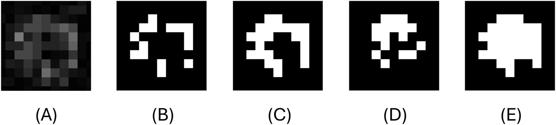
Figure 7. Example of edge detection in a particle under threshold=11. (A) is the particle after quality enhancement. (B) is the binary particle with global thresholding . (C) is the binary image after processing image B through the morphological operator. (D) is the binary particle after modified Canny Edge detection. (E) the final output of the modified Canny edge detection used in this study.
3.5 Ringing artifact removal
When parallel light beams travel through regions adjacent to high-contrast interfaces, fringe interference artifacts are prone to occur. These artifacts are frequently encountered in out-of-focus images of dense copepods and fecal pellets. Ringing artifacts are similar to Gibbs ringing that pose a significant challenge in medical imaging diagnosis as well (Yatchenko et al., 2011; Veraart et al., 2016). Various techniques exist for Gibbs artifact removal (Nasonov et al., 2007; Block et al., 2008; Krylov and Nasonov, 2008; Krylov and Nasonov, 2009; Nasonov and Krylov, 2009), and due to their similarities we can apply it to our protocol. We employed the cross-section method from the ringing level estimation of Nasonov and Krylov (2009) (Figure 8).

Figure 8. The flow chart of the Ringing artifact removal process. One major axis for each object are calculated from the longest Euclidian distance between two points along the particle edges and cross (orthogonal) lines are drawn based on that.
The method first creates a series of cross lines along the major axis of the particles, determined by identifying the two farthest points on the object’s edge. Perpendicular cross lines on each pixel along the major axis were calculated by the pixel coordinate and slope since the slope product of two perpendicular lines in a two-dimensional Cartesian plane is always -1. The primary principle in this process was to distinguish the main signal from noisy signal in each cross section along the major axis (Nasonov and Krylov, 2009). We analyzed the signal in each cross-section line using findpeaks() function to obtain both peaks and troughs as maximum gray level in each signal serves to define the main signal baseline. Essentially, the function searches for the local maximum and minimum values in a signal vector which further serves as a reference to filter out the weak sections, i.e., the part assumed to be the artifact. The signal segments continuously greater than 60% of the maximum are considered the main signal and peak signals lower than 60% are considered noises. Finally, based on the monotony of the peak signals, the nonmonotonic ones are removed since they might potentially be Gibbs artifacts (Figures 9A–D).
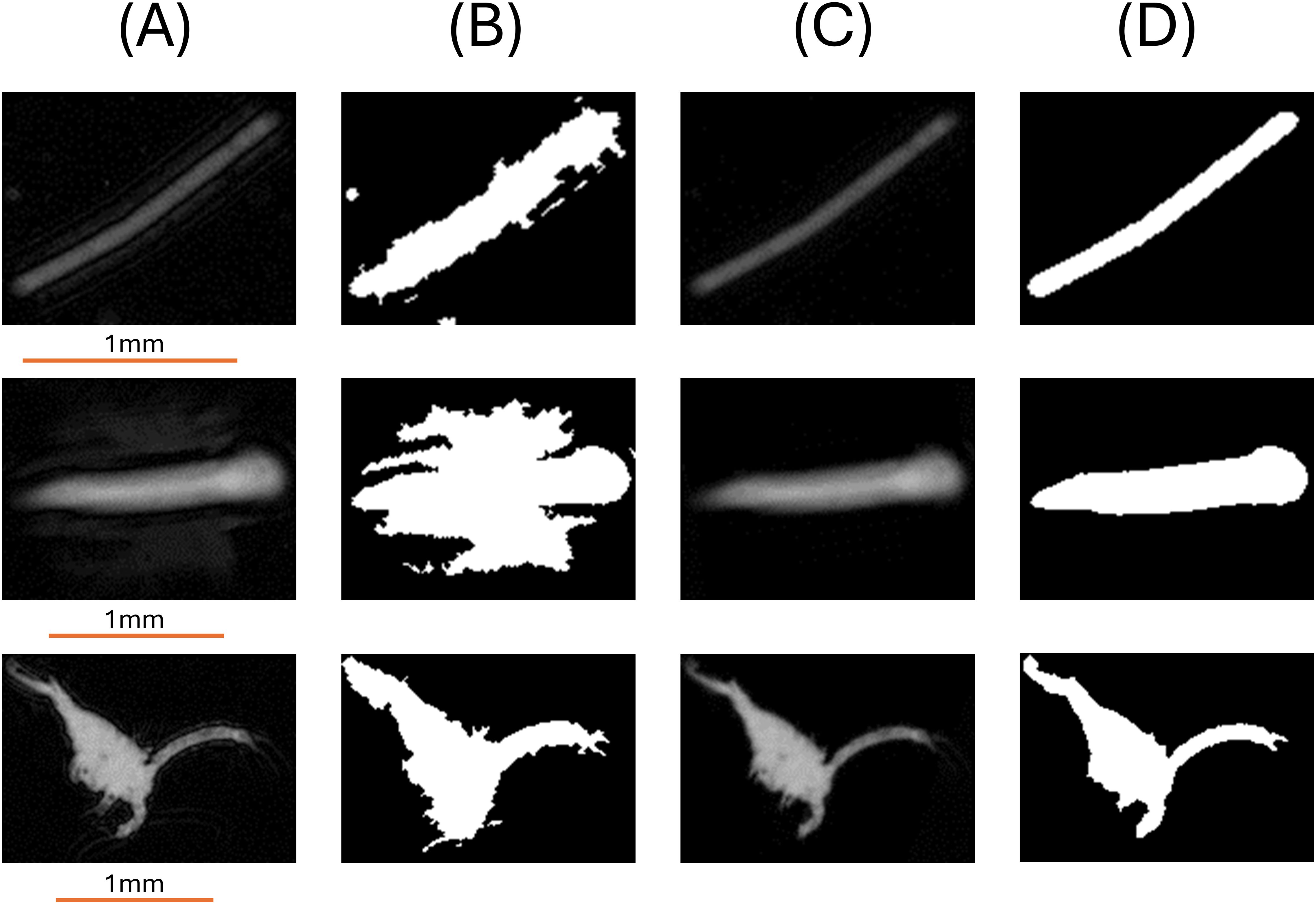
Figure 9. Example particles before and after removal of the ringing artifacts. (A) Original grayscale image, (B) original binary image, (C) grayscale image after ringing effect removal, (D) binary "deringed" image.
3.6 Special case: schlieren detection
In this section, we incorporated a preprocessing step to eliminate low-quality images ahead of the analysis owing to background distortion due to density discontinuities.
Schlieren, typically caused by inhomogeneous media such as the camera moving through pycnoclines in our case, exhibits curved structures and distorts true particle information during image binarization. It is noteworthy that schlieren are not authentic particles but rather manifestations of density differences, and simple brightness-level-based particle detection algorithms often misidentify schlieren as particles. Even the accuracy of transmissometers can be impaired by schlieren effects (Karageorgis et al., 2015). Hence these artifacts need to be removed from the dataset before further analysis. By checking our FoSI image data collected from various oceanic systems, we observed the schlieren phenomenon associated only with strong pycnoclines.
To the best of our knowledge, the impact of schlieren had only been addressed in a few in-situ image studies (Mikkelsen et al., 2008; Luo et al., 2018; Ellen et al., 2019) and discussions on schlieren detection and filtering methods are very limited, except for Luo et al. (2018). Based on the distinction of morphological characteristics between schlieren and real particles, we built two algorithms for schlieren detection.
3.6.1 Feature-based schlieren detection
Prior to schlieren detection, a reference schlieren-free image was acquired either by calculating the rolling average of a certain number of images or recording an image in clean water. Unlike the above image analysis pipeline, schlieren detection omitted the illumination correction. The first step involved numerically subtracting the reference image from the target image. Note the positive or negative signs were preserved, in which the data were not technically treated as ‘image’, since the brightness level on an image cannot be lower than 0. This was based on the observation in Figure 10A that different from the predominant real particles captured in the image, schlieren showed sections brighter than the background adjacent to features darker than the background. Following the subtraction process, the resultant grayscale images were further converted into binary images using the MicroDetect Algorithm (described in Section 2.5), with a threshold value of 0.001 in double precision. The primary strategy involves enhancing negative pixels post-subtraction (i.e., brighter than background) to find anomalies featured by schlieren. Consequently, a threshold value of 0.001 is preferred over 0 to effectively eliminate noises falling within the range of 0 to 0.001 (Figure 10C). A threshold of 0 might introduce excessive noise into the binary image, complicating the detection of schlieren structures. Objects less than 30 pixel area were removed in the subsequent step to retain only the segments representing broader schlieren effects.
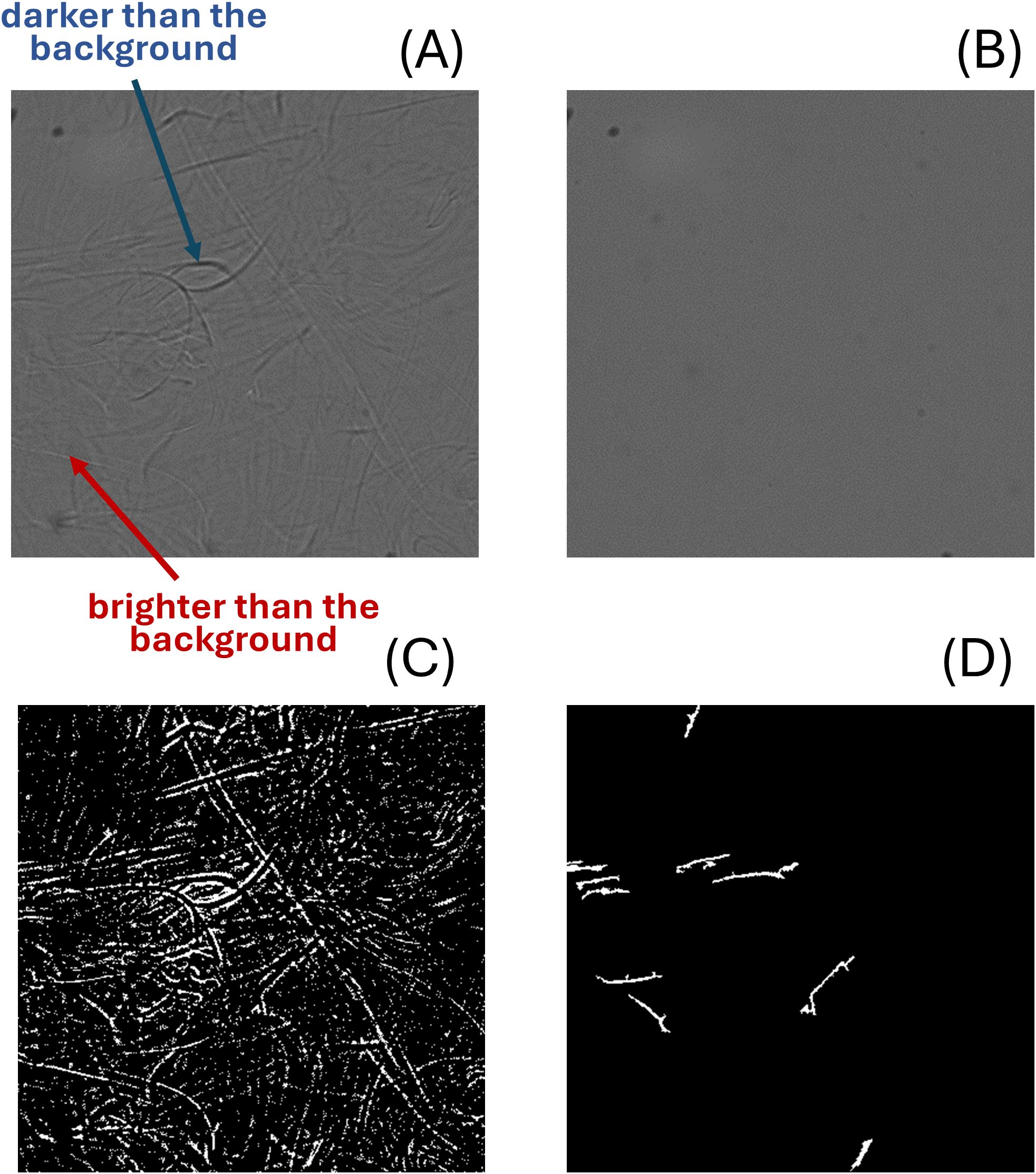
Figure 10. An example of schlieren detection (A) The raw schlieren image. (B) a blank image. (C) The binary image highlighting the negative pixels (brighter than background after subtraction). (D) The binary image after using the MicroDetect and the schlieren feature filter.
The schlieren structure filter evaluates aspect ratio and areas of each particle. We computed the former feature from the ratio of minor and major axes of an ellipse with the same normalized second central moment with the ROIs (Yuill, 1971). Specifically, the filter preserved objects exhibiting aspect ratio less than 0.2 as well as areas greater than 100 pixels². The MATLAB function regionprops() is used to determine the major and minor axis lengths. In cases when schlieren are intense and cover a large region in the image, a high-pass filter with a 40,000 pixel area threshold was introduced to capture these features instead. Following the enumeration of schlieren structures across the entire image, an image was classified as a schlieren image if there were three or more such structures present simultaneously (Figure 10D).
3.6.2 Deep learning-based schlieren detection
Transfer learning is a deep learning model widely implemented in computer vision related tasks (Ahmed et al., 2008; Simonyan and Zisserman, 2014; Bozinovski, 2020). In comparison to traditional machine learning methods, transfer learning demonstrates improved performance by achieving high prediction accuracy with minimal manual annotation (Cheplygina et al., 2019; Shaha and Pawar, 2018; Zhuang et al., 2020; Morid et al., 2021). We used transfer learning to classify schlieren patterns in addition to the feature-based detection model above.
The base model was a pretrained VGG-16, a deep learning model known for its high performance in image classification (Simonyan and Zisserman, 2014). The model was initially trained on ImageNet, a large-scale dataset comprising 20,000 types of images not including schlieren. Nevertheless, the features learned from ImageNet appeared to be transferable in the current study.
The dataset used in this study consisted of 594 images categorized into two classes: schlieren and no schlieren. This dataset was further divided into training, testing, and validation sets in a 7:1:2 ratio. The last five layers were made trainable while keeping all other layers frozen to retain the initial parameters. We froze some layers to retain the learning that has already occurred, focusing on training only the last five layers to adjust the weights for the new schlieren dataset. Unlike the typical approach of resizing images to 244 244 pixels, the original image size of 1280 960 pixels was maintained to minimize information loss. The learning rate was set at 10–5 with 50 epochs and a batch size equal to 20. The program used in the current protocol is a modified version of the Python demo provided by Elgendy (2020).
4 Results
4.1 Comparison of the particle abundance with beam attenuation (cp)
We first compared particle abundance derived from the Fall 2021 Oceanic Flux Program (OFP) cruise with the beam attenuation coefficient (cp). The results were crucial for validating our findings with respect to a widely used optical property. The cp coefficient is used as a proxy for particle concentration, particularly for particles ranging from 0.5 to 20 μm Equivalent Spherical Diameter (ESD) (Gardner et al., 2003). Our analysis from FoSI revealed a similar trend across most casts when examining particle abundance of those ranging from 24 to 50 μm ESD (Figure 11 and Figure 12; Supplementary Table 2; Supplementary Table 3). This specific size range was chosen because it is in the smaller part of the size spectrum in FoSI, and therefore more related to those observed with the transmissometer while larger particles create statistical noise due to their rarity. The scarcity of larger particles was apparent in the number spectrum analysis (Figure 13). In the epipelagic zone, the coefficient of determination (r2) of cp and FoSI particle numbers reached their highest values at thresholds between 13 to 21 with the corresponding attenuation values ranging from 0.7711 to 0.8848 across different casts (Supplementary Table 2). We also observed a slight increase in r2 values as we increased sensitivity (by lowering the threshold, see above), substantiating that the emerging particles at lower thresholds, at least down to a threshold of 21, possess characteristics beyond mere random noise. For linear regression analysis between cp and particle numbers, the p-values were smaller than 0.0001 except for cast-4 at threshold equal to 11 (Supplementary Table 2). The correlations became poorer, at thresholds < 13 in general. In addition to particle abundance, linear regression analyses of particle-projected area, total particle volume (TPV) with cp were conducted for comparison. Overall, particle area and volume parameters showed a consistent pattern in linear regression analyses. Nonetheless, the particle projected area shows the lowest r2 under same sensitivity level and cast, whereas the r2 values of TPV fell between particle abundance and area.
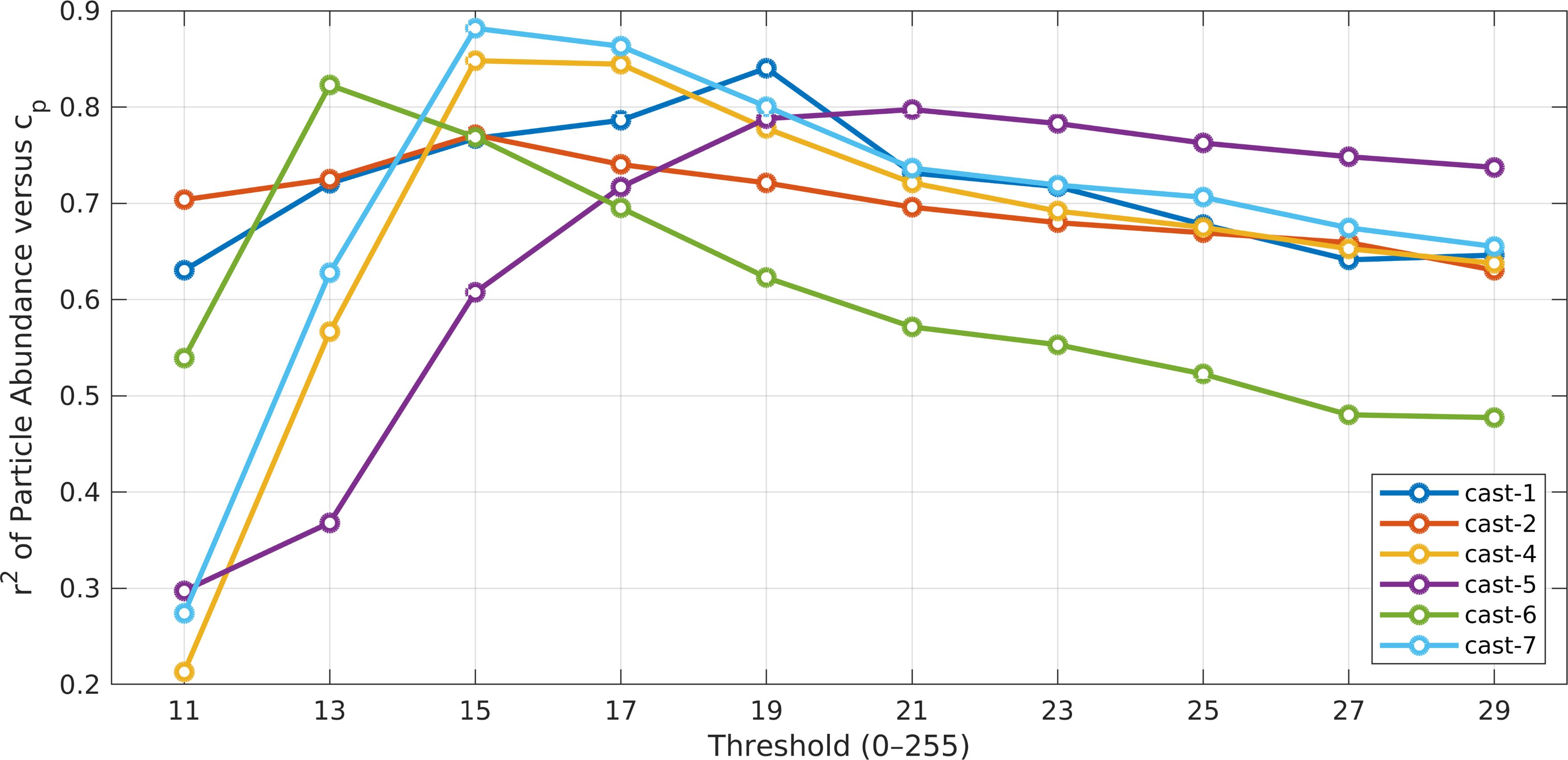
Figure 11. The coefficients of determination (r2) between particle abundance in the 22-40 µm size range and the beam attenuation coefficients (0-200 m depth range). r2 values reach their highest values at intermediate threshold (i.e., sensitivity) values.
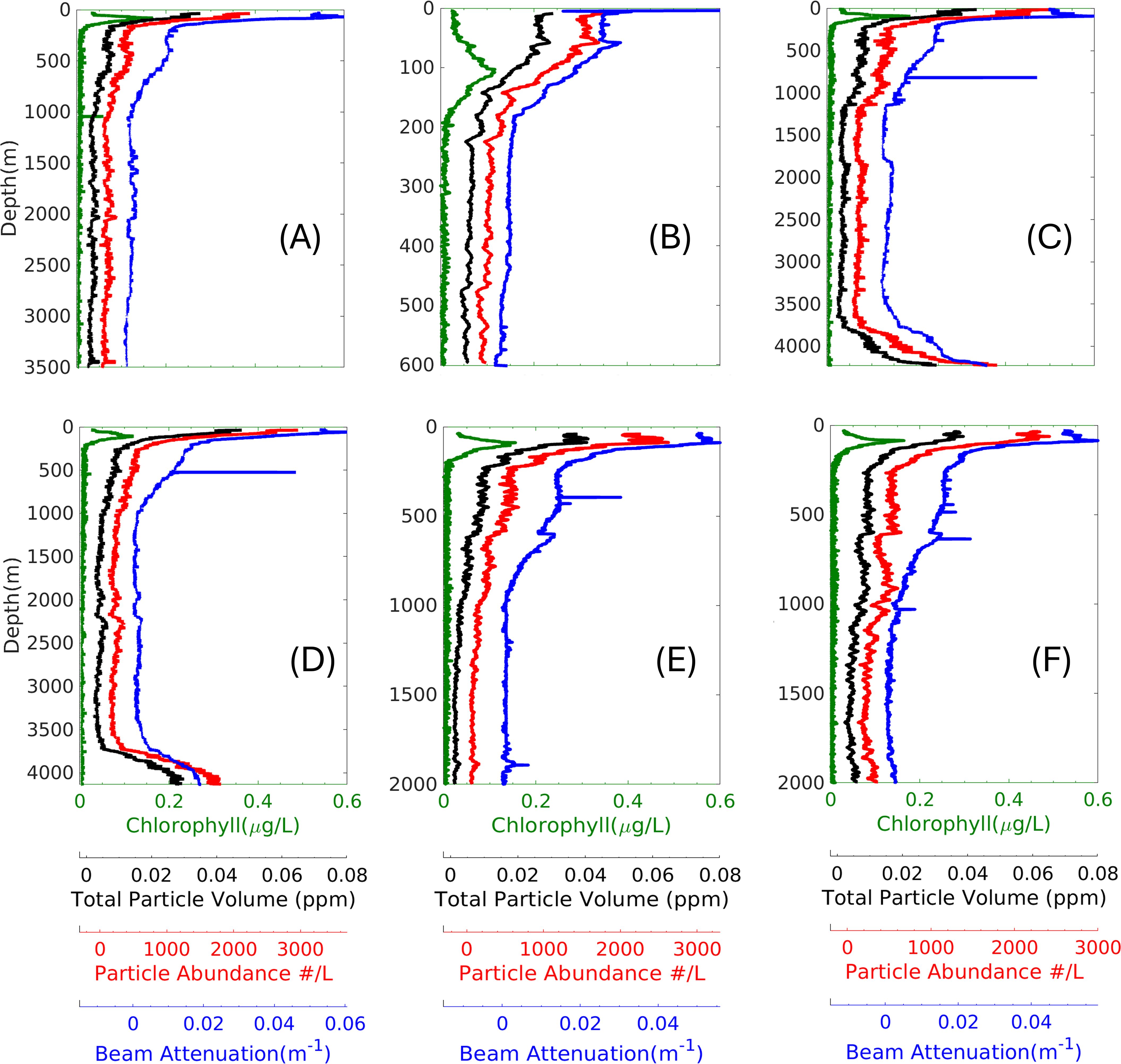
Figure 12. Vertical profiles of particle data ranging from 24-50 µm, beam attenuation, and relative chlorophyll fluorescence during the OFP October cruise. (A–F) represent cast numbers 1, 2, 4, 5, 6, and 7, respectively. Particle data were analyzed at threshold 11.
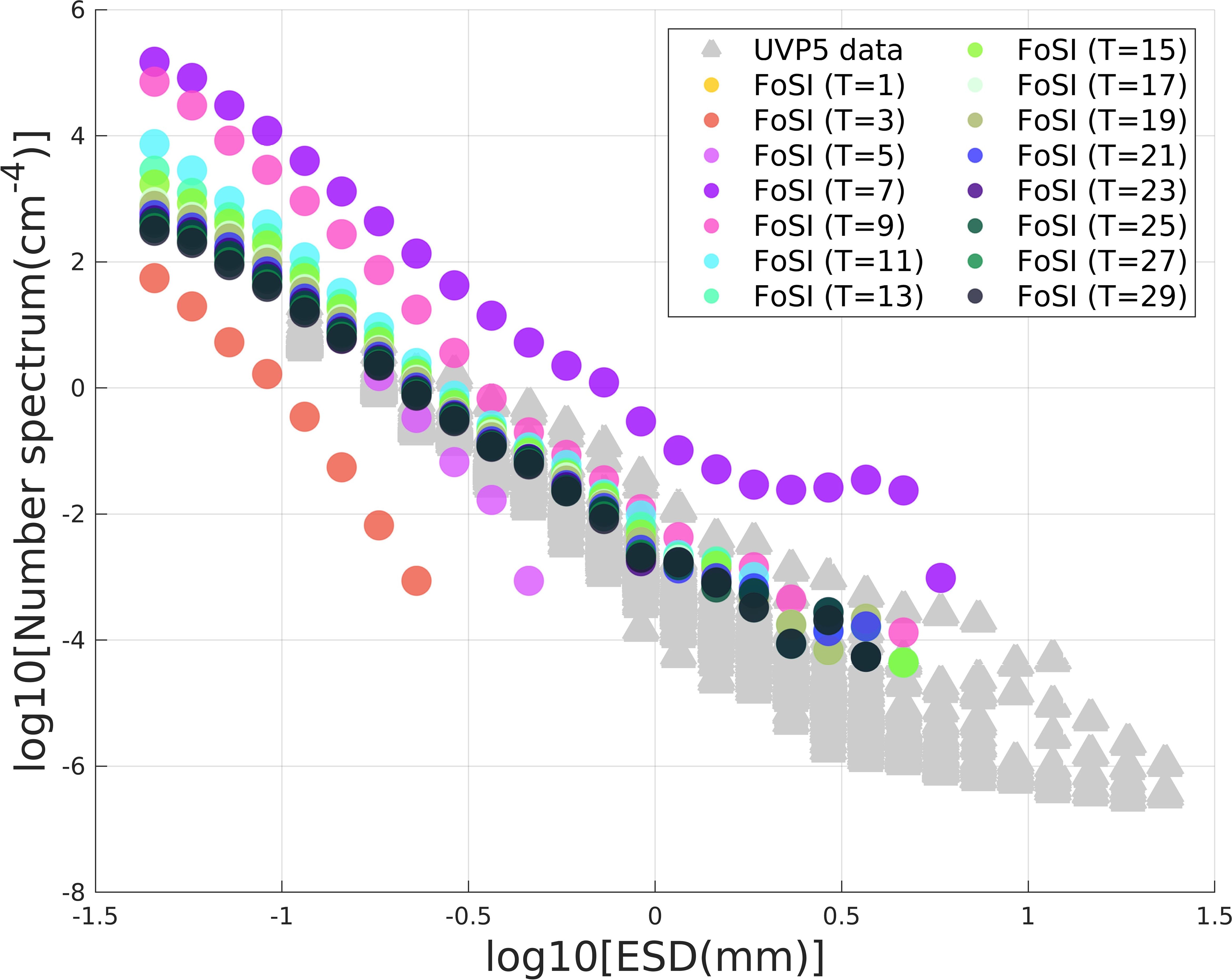
Figure 13. Number spectra of the FoSI data at various thresholds in comparison to UVP5 data from the same region (Kiko et al., 2022). The different colors represent different thresholds (i.e., sensitivities) of particle reconstruction in FoSI while the yellow lines are the particle number spectra of the UVP5.
For direct comparison, the vertical profiles of particle abundance, TPV, cp and chlorophyll data for the corresponding casts were shown in Figures 12A–F for a particle size range of 24-50 μm ESD. Particle abundance tightly correlated with cp in the epipelagic zone (<= 200m), which became weaker in the deep ocean (> 200m) where the transmissometer reached its lower dynamic range limit. We observed a peak in the particle abundance and TPV in the nepheloid layer due to resuspension (Figures 12C, D) that was simultaneously captured by the transmissometer. Chlorophyll maximum depth could be found in the surface layer; however, the chlorophyll concentration rapidly dropped to undetectable levels in the mesopelagic zone. Notably, the Chlorophyll maximum depth aligned with particle abundance peak in some but not all casts.
4.2 Reconstruction of gel-type particles
To investigate how the MicroDetect algorithm performed on recognizing the transparent particle fraction, we compared the binary image processed by global thresholding and our algorithm at a high sensitivity level (threshold = 13, corresponding to OD=0.1681 based on Figure 5 and Supplementary Table 1). The results showed that the MicroDetect algorithm is capable of recognizing the gel-like portion of inhomogeneous particles, such as marine snow, Rhizaria and Appendicularia, the transparent fraction of which are almost undetectable using the global thresholding method (Figure 14). In Figure 14A, the MicroDetect Algorithm not only captured the transparent gel matrices of marine snow particles but also identified fragmented small particles as part of larger irregular aggregates. The enhancement seen with MicroDetect Algorithm suggested its capacity in terms of recognizing transparent particle features in the ocean environment, accounting for more accurate particle reconstruction at the same sensitivity level. It is noteworthy that the goal was not to highlight detailed features in the particles but to arrive at a more accurate representation of the true particle dimensions. The accurate rendering of larger connected particles is important as it influences the slopes of particle size spectra. Another possible solution for this problem is density-based spatial clustering as suggested by Bochdansky et al. (2022).
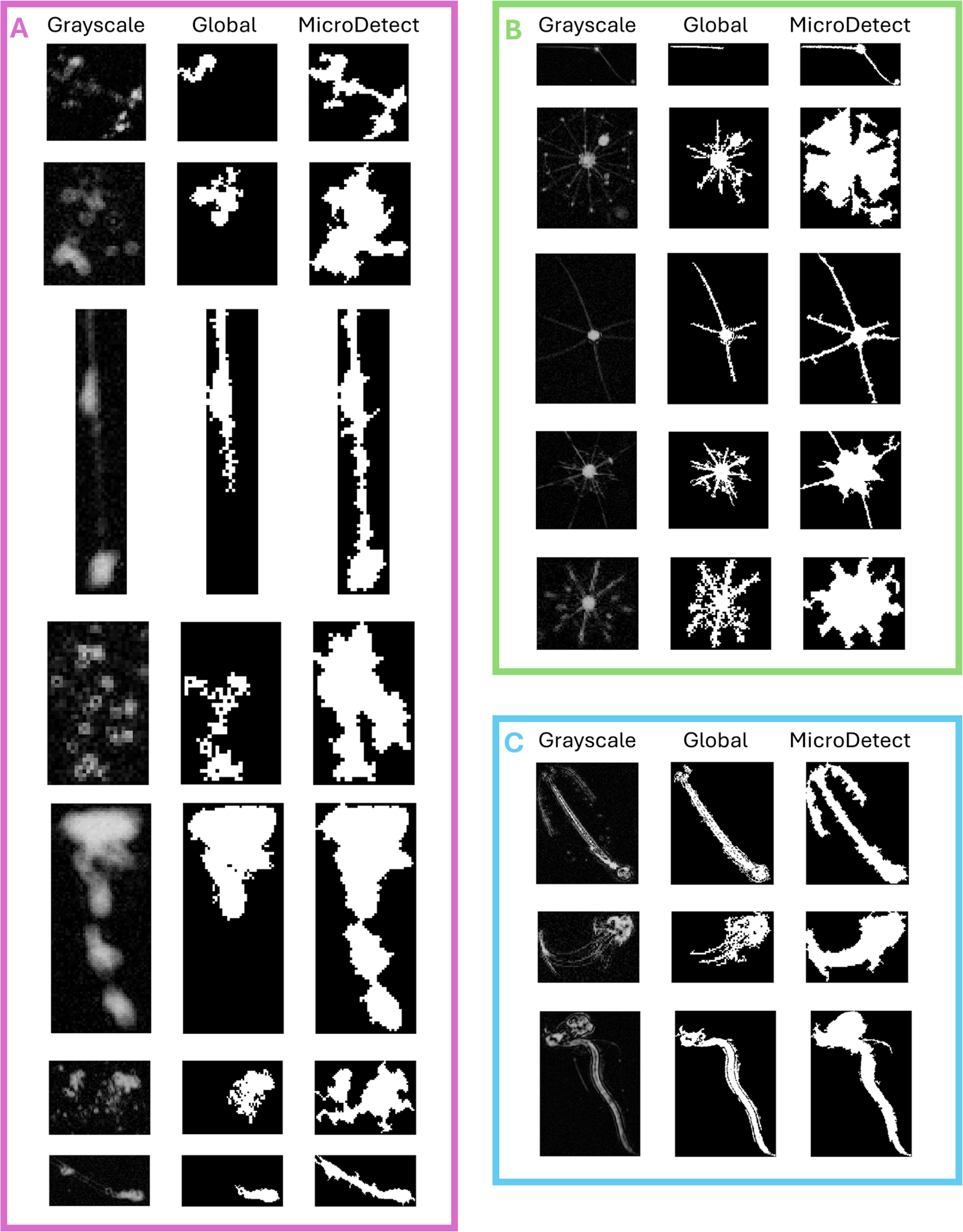
Figure 14. The ROI segmentation results comparing the traditionally used global thresholding with our new edge detection algorithm. (A) marine snow, (B) Rhizaria, (C) Appendicularia. The global thresholding method only identifies a fraction of the particles, underscoring the advantage of our edge detection technique. Unlike simple thresholding, our method can discern fainter portions of a particle even at the same threshold level. Note the particle images in the figures are not to scale.
4.3 Comparison of particle number spectra between FoSI and UVP5 data collected in the same region
We defined 28 particle size classes within the range of 0.0403 millimeters to 26 millimeters as in Kiko et al., 2022. This analysis used the particle data from the upper 400 m collected in spring 2021 during an Oceanic Flux Program (OFP) cruise.The particle number spectra were created using Equation 10 described in Jackson et al. (1997),
where n refers to the particle number spectrum, Su refers to the upper value of the size class. Sl refers to the lower value of the size class. Vsamp represents the sample volume. The particle number spectrum represents the number of particles in each size class, divided by the size class width and sample volume (Jackson et al., 1997). FoSI and UVP5 were deployed at the same site but different years (Figure 13). The elevation of the FoSI particle number spectra was substantially higher than the UVP5 except for two casts (Figure 13) indicating that shadowgraph imaging is capable of detecting more particles especially those with low OD. While the threshold selected for UVP spectrum analysis is unknown, the particle numbers detected by FoSI at threshold equivalent to 7 (OD= 0.1168) fall approximately two orders of magnitude higher than the UVP spectra (Figure 13).
5 Discussion
The method described in this paper presented a detailed image analysis pipeline primarily designed for shadowgraph imaging. In contrast to other existing image analysis algorithms, our method more efficiently extracted information to small and low-optical-density particles from in-situ images. The accurate particle recognition protocol will support studies that require high-resolution data as a solid foundation to further investigate the biological significance of aquatic particles (Verdugo et al., 2004; Giering et al., 2020a; Irby et al., 2024; Huang et al., 2024).
The illumination correction involved the simple flat fielding method devoid of histogram equalization, as any change in image contrast may alter the preceding calibration model. Overcorrection occurred when some pixels in an image are extremely bright (close to 255) or dark (close to 0) (Xu et al., 2010). Piccinini and Bevilacqua, 2018 described a method to avoid overcorrection by maintaining all the pixels with 255 unchanged in the image before and after illumination correction. To resolve this issue in our protocol, we added an artifact mask to exclude those overcorrected pixels. Similarly, illumination correction has been applied to effectively acquire clean particle data in microscopic images (Leong et al., 2003).
Changes in OD are explicitly observed in shadowgraph imaging systems because the configurations enable us to identify this difference. A similar calibration is not feasible with other optical systems such as LISST which are based on scatter, and which lack the capacity to recognize this variation. Threshold calibration offers objective comparison across different camera settings accompanied by an explicit absolute OD value. Having a precise OD value that determines the analytic threshold provides an objective reference (OD) that makes the results comparable. As previously discussed (Bochdansky et al., 2022), the threshold selection process is highly arbitrary when particles are extracted from in-situ images and few researchers aware that varying these thresholds can result in differences of several orders of magnitude in the estimated particle abundance (Figure 13).
Image subtraction is a simple yet critical step in image processing (Oberholzer et al., 1996; Russ, 2006). Gray levels in an image cannot be negative, meaning the image subtraction always results in a positive value. Meanwhile, even if the probability of overlap is low in oligotrophic environments (Conte et al., 2001; Gundersen et al., 2001), absolute subtraction might cause some errors when particles in two consecutive images overlap on the same pixel regions. In cases of high particle concentrations such as estuarine and coastal systems, we recommend filming deionized water images taken either before or after the cast as reference or by physically decreasing the imaging gap between light source and the camera housing to decrease the image volume. In oligotrophic systems such as in the Sargasso Sea and in deep sea environments as shown here, particles are so rare that particle overlaps are a statistically negligible problem.
In shadowgraphs, particles are typically darker than the background, but few exceptions arose during the analysis as we occasionally observed gel-like particles brighter than the background seawater, which was also observed in the presence of schlieren (Figure 10). Most marine particles are known to be of higher OD than the surrounding seawater (Mobley, 2022). However, it is conceivable that gels as well as density discontinuities such as schlieren lead to a lensing effect in which light is concentrated in certain small regions of the image sensor.
In our search for an effective algorithm to analyze millions of small particles from large datasets, we conducted experiments on various edge detection methods, ranging from local thresholding to more complex techniques. Our analysis corroborated results of a previous study on particle detection techniques (Giering et al., 2020b). For example, using Canny detection alone tends to fragment large particles and introduce significant Gibbs ring artifacts. The noises around the large particles are likely to be amplified by Canny detection as wiggly lines. Under the same threshold, Canny detection was found to overestimate particle size, while other algorithms, such as Prewitt and Roberts edge detection (Roberts, 1963; Prewitt, 1970), struggled to detect faint particles (Supplementary Figure 5). Although the Otsu method (Otsu, 1975) automatically determines the threshold based on brightness variation, it had been proved less effective for detecting small, faint particles (Cai et al., 2014; Yuan et al., 2016). In contrast to the algorithms above, our MicroDetect Algorithm was derived from the Canny edge detection algorithm as described by Nayak et al., 2015. To tailor the original algorithm for particle analysis, we eliminated the morphological opening filter, which tends to inflate particle size in our application. Additionally, we removed edges detected by the Canny method after filling in holes to minimize overestimation Figures 7A–E. Although machine learning algorithms are known for their effectiveness in image edge detection (Arteta et al., 2012; Irisson et al., 2022; Panaïotis et al., 2022; Yao et al., 2022), we believe that the MicroDetect Algorithm can be exceptionally practical for image classification following the ROI segmentation, hence decided to set aside the computationally expensive techniques.
The proposed feature-based schlieren detection can be programmed with relatively simple functions. Nevertheless, the applicability of our schlieren detection algorithm is limited to evenly illuminated images. When dealing with image data influenced by severely uneven illumination, the algorithm may fail. Another drawback is attributed to the area filter used to exclude schlieren, which may falsely eliminate large particles with high-aspect ratio, e.g., large medusae, some elongated marine snow particles, diatom chain or marine snow debris (Bochdansky et al., 2016). By contrast, the deep learning-based schlieren detection outperforms in terms of accuracy while the outputs depend largely on data quality during training. Since the training image set requires update when it is applied to a new camera setting, the manual selection and training greatly increase the complexity of the process.
Several studies made intercomparisons of particle parameters measured by different optical instruments. The study of Behrenfeld and Boss (2006) showed a high correlation at upper 200 m North Pacific of Coulter Counter-based particle (~1.5-40μm) data and cp (r2 = 0.77) which compares well with the results presented in the current study (Supplementary Table 2). The spikes in the cp were not seen in the FoSI data (Figure 12), because they are rare large particles that pass through the light beam of the transmissometer (Briggs et al., 2013; Giering et al., 2020a). Our results resembled a LISST-100 study suggesting cp is less sensitive to the change of particle size and correlates better with particle abundance than TPV (Boss et al., 2009). Another study inferred particle projected area reflects cp better than TPV because the particles are imaged as two-dimensional projections (Hill et al., 2011), however, we did not observe this in FoSI data. Our results showed that the correlations ranked with cp as particle abundance > TPV > particle projected area (Supplementary Tables 2, 3). Additionally, the statistical results indicate that higher sensitivity levels lead to a stronger correlation between cp and particle abundance for particles ranging from 22 to 40 μm, with the r2 peaking at thresholds between 13 and 19 (see Supplementary Table 1 for the corresponding OD values).
We selected marine snow, Rhizaria and Appendicularia to represent particles containing transparent features that sometimes lead to fragmentation during image analysis. Marine snow particles include aggregates greater than 0.5 millimeter that contain transparent gel matrices. Previous investigations revealed the unique, yet elusive characteristics of marine snow based on optical and fluid mechanical observations (Honjo et al., 1984; Petrik et al., 2013; Markussen et al., 2020; Chajwa et al., 2024; Cael and Guidi, 2024). Chajwa et al. (2024) visualized the mucus comet-tails on sinking marine snow particles with high-resolution Particle Image Velocimetry (PIV) and further inferred that the optically invisible fraction of marine snow visualized via the flow field around the particles contributed greatly to the particle size and their sinking velocity. While not perfect, our MicroDetect Algorithm recognized at least a large portion of the mucus matrix (Figure 14A). As the particle size increases, one may assume that sinking velocity of these particles increases according to Stoke’s law. However, it appeared that this is not universally true (Iversen and Lampitt, 2020). Since the gels are neutrally or even positively buoyant (Azetsu-Scott and Passow, 2004; Engel, 2009; Mari et al., 2017; Romanelli et al., 2023), they reduce the particle sinking velocities as clearly demonstrated by Chajwa et al. (2024). This indicates that for the same image data, the improved object detection algorithm will extract more information on the potential sinking velocity of particles. Rhizaria are a group of protists abundant in the mesopelagic zone. Studying them has been challenging owing to their fragile structure and easily being dissolved in fixatives (Matsuzaki et al., 2015; Nakamura et al., 2015; Biard et al., 2015, 2018; Biard and Ohman, 2020; Mars Brisbin et al., 2020). Consequently, researchers use in situ optical devices (Biard et al., 2016, 2018; Nakamura et al., 2017; Biard et al., 2020; Mars Brisbin et al., 2020). The MicroDetect Algorithm detects the endoplasm and spicules of Radiolaria as well as the much more transparent ectoplasm that harbors algae and food vacuoles and is difficult to detect by most photographic systems (Ohtsuka et al., 2015) (Figure 14B).
Similarly, Appendicularia and Cnidaria, both broadly distributed zooplankton worldwide (Cairns, 1992; Båmstedt et al., 2005; Capitanio et al., 2008; Kodama et al., 2018; Williams, 2011) exhibit transparent features in their bodies that are not rendered well with conventional image analysis tools but are better outlined using the MicroDetect Algorithm (Figure 14C). However, FoSI cannot visualize the entire transparent structures on Appendicularian houses even at higher sensitivities (Bochdansky et al., 2022). While the MicroDetect Algorithm more accurately recovered their actual sizes, the loss of image details will hinder the taxonomic identification of these plankter. In fact, the ROIs extracted from the original gray scale images will be a better fit than the binary images in terms of identification using machine learning algorithms.
In conclusion, this paper provides a detailed step-by-step workflow for the analysis of oceanographic images from a shadowgraph system. The primary advancement of our method involved the development of the MicroDetect Algorithm to better reconstruct the ocean particles from 24 to 500 μm. Additionally, the novel protocol significantly improved the recognition of gel-like structures in the water column and transparent parts of plankton organisms. This highlights potential new approaches for studies of the oceanic gel phase independent of traditional Alcian Blue staining methods. Finally, we addressed the most vexing problems in image analysis and hope that by the application of neutral density filters as presented here, a standardization of different shadowgraph cameras can be achieved in the future.
Data availability statement
The raw data supporting the conclusions of this article will be made available by the authors, without undue reservation.
Author contributions
HH: Conceptualization, Data curation, Formal Analysis, Investigation, Methodology, Software, Validation, Visualization, Writing – original draft, Writing – review & editing. AB: Conceptualization, Data curation, Funding acquisition, Project administration, Resources, Supervision, Validation, Writing – review & editing.
Funding
The author(s) declare that financial support was received for the research and/or publication of this article. This project was supported by the Natural Science Fundation (NSF) under Grant #2128438.
Acknowledgments
We thank Maureen Conte (Bermuda Institute of Ocean Sciences), Rut Pedrosa Pàmies (Marine Biological Laboratory, Woods Hole) and the crew of the RV Atlantic Explorer for their kind support.
Conflict of interest
The authors declare that the research was conducted in the absence of any commercial or financial relationships that could be construed as a potential conflict of interest.
Generative AI statement
The author(s) declare that no Generative AI was used in the creation of this manuscript.
Publisher’s note
All claims expressed in this article are solely those of the authors and do not necessarily represent those of their affiliated organizations, or those of the publisher, the editors and the reviewers. Any product that may be evaluated in this article, or claim that may be made by its manufacturer, is not guaranteed or endorsed by the publisher.
Supplementary material
The Supplementary Material for this article can be found online at: https://www.frontiersin.org/articles/10.3389/fmars.2025.1539828/full#supplementary-material
References
Abdelsalam D. G. and Kim D. (2011). Coherent noise suppression in digital holography based on flat fielding with apodized apertures. Optics Express 19, 17951–17959. doi: 10.1364/OE.19.017951
Ahmed A., Yu K., Xu W., Gong Y., and Xing E. (2008). “Training hierarchical feed-forward visual recognition models using transfer learning from pseudo-tasks,” in Computer Vision–ECCV 2008: 10th European Conference on Computer Vision, vol. 10. (Springer Berlin Heidelberg, Marseille, France), 69–82. Proceedings, Part III.
Arteta C., Lempitsky V., Noble J. A., and Zisserman A. (2012). “Learning to detect cells using non-overlapping extremal regions,” in Medical Image Computing and Computer-Assisted Intervention–MICCAI 2012: 15th International Conference, vol. 15. (Springer Berlin Heidelberg, Nice, France), 348–356. Proceedings, Part I.
Azetsu-Scott K. and Passow U. (2004). Ascending marine particles: Significance of transparent exopolymer particles (TEP) in the upper ocean. Limnology oceanography 49, 741–748. doi: 10.4319/lo.2004.49.3.0741
Båmstedt U., Fyhn H. J., Martinussen M. B., Mjaavatten O., and Grahl-Nielsen O. (2005). Seasonal distribution, diversity and biochemical composition of Appendicularians in Norwegian fjords. Response of marine ecosystem to global change: ecological impact of Appendicularians. GB Sci. Publisher, 233–259.
Beer. (1852). Bestimmung der Absorption des rothen Lichts in farbigen Flüssigkeiten. Annalen der Physik, 162 (5), 78-88.
Behrenfeld M. J. and Boss E. (2006). Beam attenuation and chlorophyll concentration as alternative optical indices of phytoplankton biomass. J. Mar. Res. 64, 431–451. doi: 10.1357/002224006778189563
Biard T., Krause J. W., Stukel M. R., and Ohman M. D. (2018). The significance of giant Phaeodarians (Rhizaria) to biogenic silica export in the California Current Ecosystem. Global Biogeochemical Cycles 32, 987–1004. doi: 10.1029/2018GB005877
Biard T. and Ohman M. D. (2020). Vertical niche definition of test-bearing protists (Rhizaria) into the twilight zone revealed by in situ imaging. Limnology Oceanography 65, 2583–2602. doi: 10.1002/lno.11472
Biard T., Pillet L., Decelle J., Poirier C., Suzuki N., and Not F. (2015). Towards an integrative morpho-molecular classification of the Collodaria (Polycystinea, Radiolaria). Protist 166, 374–388. doi: 10.1016/j.protis.2015.05.002
Biard T., Stemmann L., Picheral M., Mayot N., Vandromme P., Hauss H., et al. (2016). In situ imaging reveals the biomass of giant protists in the global ocean. Nature 532, 504–507. doi: 10.1038/nature17652
Block K. T., Uecker M., and Frahm J. (2008). Suppression of MRI truncation artifacts using total variation constrained data extrapolation. Int. J. Biomed. Imaging 2008. doi: 10.1155/2008/184123
Bochdansky A. B., Clouse M. A., and Herndl G. J. (2016). Dragon kings of the deep sea: marine particles deviate markedly from the common number-size spectrum. Sci. Rep. 6, 1–7. doi: 10.1038/srep22633
Bochdansky A. B., Huang H., and Conte M. H. (2022). The aquatic particle number quandary. Front. Mar. Sci. 9, 994515. doi: 10.3389/fmars.2022.994515
Bochdansky A. B., Jericho M. H., and Herndl G. J. (2013). Development and deployment of a point-source digital inline holographic microscope for the study of plankton and particles to a depth of 6000 m. Limnology Oceanography: Methods 11, 28–40. doi: 10.4319/lom.2013.11.28
Boss E., Slade W., and Hill P. (2009). Effect of particulate aggregation in aquatic environments on the beam attenuation and its utility as a proxy for particulate mass. Optics Express 17, 9408–9420.
Bozinovski S. (2020). Reminder of the first paper on transfer learning in neural networks 1976. Informatica 44, 291–302. doi: 10.31449/inf.v44i3.2828
Bradley D. and Roth G. (2007). Adaptive thresholding using the integral image. J. Graphics Tools 12, 13–21. doi: 10.1080/2151237X.2007.10129236
Briggs N. T., Slade W. H., Boss E., and Perry M. J. (2013). Method for estimating mean particle size from high-frequency fluctuations in beam attenuation or scattering measurements. Appl. Optics 52, 6710–6725. doi: 10.1364/AO.52.006710
Cael B. B. and Guidi L. (2024). Tiny comets under the sea. Science 386, 149–150. doi: 10.1126/science.ads5642
Cai H., Yang Z., Cao X., Xia W., and Xu X. (2014). A new iterative triclass thresholding technique in image segmentation. IEEE Trans. image Process. 23, 1038–1046. doi: 10.1109/TIP.83
Cairns S. D. (1992). Worldwide distribution of the stylasteridae (Cnidaria: Hydrozoa). Scientia Marina.
Canny J. (1986). A computational approach to edge detection. IEEE Trans. Pattern Anal. Mach. Intell. 6), 679–698. doi: 10.1109/TPAMI.1986.4767851
Capitanio F. L., Curelovich J., Tresguerres M., Negri R. M., Delia Viñas M., and Esnal G. B. (2008). Seasonal Cycle of Appendicularians at a Coastal Station (38° 28′ s, 57° 4′ w) of the SW Atlantic Ocean. Bull. Mar. Sci. 82, 171–184.
Chajwa R., Flaum E., Bidle K. D., Van Mooy B., and Prakash M. (2024). Hidden comet-tails of marine snow impede ocean-based carbon sequestration. arXiv preprint arXiv:2310.01982 386 (6718), eadl5767. doi: 10.1126/science.adl576
Cheng X., Cheng K., and Bi H. (2020a). Dynamic downscaling segmentation for noisy, low-contrast in situ underwater plankton images. IEEE Access 8 (9), 111012–111026. doi: 10.1109/Access.6287639
Cheng X., Ren Y., Cheng K., Cao J., and Hao Q.. (2020b). Method for training convolutional neural networks for in situ plankton image recognition and classification based on the mechanisms of the human eye. Sensors 20 (9), 2592. doi: 10.3390/s20092592
Cheplygina V., De Bruijne M., and Pluim J. P. (2019). Not-so-supervised: a survey of semi-supervised, multi-instance, and transfer learning in medical image analysis. Med. image Anal. 54, 280–296. doi: 10.1016/j.media.2019.03.009
Choi S. M., Seo J. Y., Ha H. K., and Lee G. H. (2018). Estimating effective density of cohesive sediment using shape factors from holographic images. Estuarine Coast. Shelf Sci. 215, 144–151. doi: 10.1016/j.ecss.2018.10.008
Conte M. H., Ralph N., and Ross E. H. (2001). Seasonal and interannual variability in deep ocean particle fluxes at the Oceanic Flux Program (OFP)/Bermuda Atlantic Time Series (BATS) site in the western Sargasso Sea near Bermuda. Deep Sea Res. Part II: Topical Stud. Oceanography 48, 1471–1505. doi: 10.1016/S0967-0645(00)00150-8
Cowen R. K. and Guigand C. M. (2008). An operational in situ ichthyoplankton imaging system (ISIIS). OceanObs. doi: 10.4319/lom.2008.6.126
Daniels J., Sainz G., and Katija K. (2023). New method for rapid 3D reconstruction of semi-transparent underwater animals and structures. Integr. Organismal Biol. 5, obad023. doi: 10.1093/iob/obad023
Davis C. S., Gallager S. M., Berman M. S., Haury L. R., and Strickler J. R. (1992). The Video Plankton Recorder (VPR): design and initial results. Arch. Hydrobiol. Beih 36, 67–81.
Davis C. S., Thwaites F. T., Gallager S. M., and Hu Q. (2005). A three-axis fast-tow digital Video Plankton Recorder for rapid surveys of plankton taxa and hydrography. Limnology Oceanography: Methods 3, 59–74. doi: 10.4319/lom.2005.3.59
de Lange S. I., Sehgal D., Martínez-Carreras N., Waldschläger K., Bense V., Hissler C., et al. (2024). The impact of flocculation on in situ and ex situ particle size measurements by laser diffraction. Water Resour. Res. 60, e2023WR035176.
Durkin C. A., Buesseler K. O., Cetinić I., Estapa M. L., Kelly R. P., and Omand M. (2021). A visual tour of carbon export by sinking particles. Global Biogeochemical Cycles 35, e2021GB006985. doi: 10.1029/2021GB006985
Ellen J. S., Graff C. A., and Ohman M. D. (2019). Improving plankton image classification using context metadata. Limnology Oceanography: Methods 17, 439–461. doi: 10.1002/lom3.10324
Emerson G. P. and Little S. J. (1999). Flat-fielding for CCDs in AAVSO observations, I. J. Am. Assoc. Variable Star Observers 27, 49–54.
Engel A. (2009). “Determination of marine gel particles,” in Practical guidelines for the analysis of seawater (CRC Press), 125–142.
Gardner W. D., Mishonov A. V., and Richardson M. J. (2003). “Global POC synthesis using ocean color measurement calibrated with JGOFS and WOCE data on beam attenuation and POC,” in EGS-AGU-EUG Joint Assembly. 12905.
Giering S. L. C., Cavan E. L., Basedow S. L., Briggs N., Burd A. B., Darroch L. J., et al. (2020a). Sinking organic particles in the ocean—flux estimates from in situ optical devices. Front. Mar. Sci. 6, 834. doi: 10.3389/fmars.2019.00834
Giering S. L., Hosking B., Briggs N., and Iversen M. H. (2020b). The interpretation of particle size, shape, and carbon flux of marine particle images is strongly affected by the choice of particle detection algorithm. Front. Mar. Sci. 7, 564. doi: 10.3389/fmars.2020.00564
Gorsky G., Aldorf C., Kage M., Picheral M., Garcia Y., and Favole J. (1992). Vertical distribution of suspended aggregates determined by a new underwater video profiler. In Annales de lInstitut océanographique 68 (1-2), 275–280.
Gorsky G., Ohman M. D., Picheral M., Gasparini S., Stemmann L., Romagnan J. B., et al. (2010). Digital zooplankton image analysis using the ZooScan integrated system. J. plankton Res. 32, 285–303. doi: 10.1093/plankt/fbp124
Greer A. T., Duffy P. I., Walles T. J., Cousin C., Treible L. M., Aaron K. D., et al. (2025). Modular shadowgraph imaging for zooplankton ecological studies in diverse field and mesocosm settings. Limnology Oceanography: Methods 23, 67–86. doi: 10.1002/lom3.10657
Gundersen K., Orcutt K. M., Purdie D. A., Michaels A. F., and Knap A. H. (2001). Particulate organic carbon mass distribution at the Bermuda Atlantic Time-series Study (BATS) site. Deep Sea Res. Part II: Topical Stud. Oceanography 48, 1697–1718. doi: 10.1016/S0967-0645(00)00156-9
Hill P. S., Boss E., Newgard J. P., Law B. A., and Milligan T. G. (2011). Observations of the sensitivity of beam attenuation to particle size in a coastal bottom boundary layer. J. Geophys. Res.: Oceans 116.
Honjo S., Doherty K. W., Agrawal Y. C., and Asper V. L. (1984). Direct optical assessment of large amorphous aggregates (marine snow) in the deep ocean. Deep Sea Res. Part A. Oceanographic Res. Papers 31, 67–76. doi: 10.1016/0198-0149(84)90073-6
Huang H., Ezer T., and Bochdansky A. B. (2024). Biological-physical interaction of particle distribution: the turbulent mixed-layer pump and particle sinking explored through modeling and observations. In American Geophysical Union, Ocean Sciences Meeting. 2134, PS34D–2134. Available online at: https://ui.adsabs.harvard.edu/abs/2024AGUOSPS34D2134H/abstract
Iversen M. H. and Lampitt R. S. (2020). Size does not matter after all: No evidence for a size-sinking relationship for marine snow. Prog. Oceanogr. 189, 102445. doi: 10.1016/j.pocean.2020.102445
Irby M. S., Huang H., and Bochdansky A. B. (2024). Classification of plankton and particulate matter from the north Atlantic based on shadowgraph images from an underwater microscope. ODU knowledge EXPO. Available online at: https://digitalcommons.odu.edu/undergradsymposium/2024/posters/8/
Irisson J. O., Ayata S. D., Lindsay D. J., Karp-Boss L., and Stemmann L. (2022). Machine learning for the study of plankton and marine snow from images. Annu. Rev. Mar. Sci. 14, 277–301. doi: 10.1146/annurev-marine-041921-013023
Jackson G. A. and Checkley J. D.M. (2011). Particle size distributions in the upper 100 m water column and their implications for animal feeding in the plankton. Deep Sea Res. Part I: Oceanographic Res. Papers 58 (3), 283–297. doi: 10.1016/j.dsr.2010.12.008
Jackson G. A., Maffione R., Costello D. K., Alldredge A. L., Logan B. E., and Dam H. G. (1997). Particle size spectra between 1 μm and 1 cm at Monterey Bay determined using multiple instruments. Deep Sea Res. Part I: Oceanographic Res. Papers 44, 1739–1767.
Karageorgis A., Georgopoulos D., Gardner W., Mikkelsen O., and Velaoras D. (2015). How schlieren affects beam transmissometers and LISST-Deep: an example from the stratified Danube River delta, NW Black Sea. Mediterranean Marine Sci. 16, 366–372.
Kiko R., Picheral M., Antoine D., Babin M., Berline L., Biard T., et al. (2022). A global marine particle size distribution dataset obtained with the Underwater Vision Profiler 5. Earth System Sci. Data Discussions 2022, 1–37. doi: 10.5194/essd-14-4315-2022
Kim J. Y., Kim J. W., Seo S. H., Kye Y. C., and Ahn H. H. (2011). A novel consistent photomicrography technique using a reference slide made of neutral density filter. Microscopy Res. Technique 74, 397–400. doi: 10.1002/jemt.20921
Kodama T., Iguchi N., Tomita M., Morimoto H., Ota T., and Ohshimo S. (2018). Appendicularians in the southwestern Sea of Japan during the summer: abundance and role as secondary producers. J. Plankton Res. 40, 269–283. doi: 10.1093/plankt/fby015
Krylov A. and Nasonov A. (2008). “Adaptive total variation deringing method for image interpolation,” in 2008 15th IEEE International Conference on Image Processing. 2608–2611 (IEEE).
Krylov A. S., Nasonov A. V., and Chernomorets A. A. (2009). “Combined linear resampling method with ringing control,” in Proceedings of GraphiCon, Vol. 2009. 163–165.
Leong F. W., Brady M., and McGee J. O. D. (2003). Correction of uneven illumination (vignetting) in digital microscopy images. J. Clin. Pathol. 56, 619–621. doi: 10.1136/jcp.56.8.619
Li E., Saggiomo V., Ouyang W., Prakash M., and Diederich B. (2024). ESPressoscope: A small and powerful approach for in situ microscopy. PloS One 19, e0306654. doi: 10.1371/journal.pone.0306654
Lie W. N. (1995). Automatic target segmentation by locally adaptive image thresholding. IEEE Trans. Image Process. 4, 1036–1041. doi: 10.1109/83.392347
Luo J. Y., Irisson J. O., Graham B., Guigand C., Sarafraz A., Mader C., et al. (2018). Automated plankton image analysis using convolutional neural networks. Limnology Oceanography: Methods 16 (12), 814–827. doi: 10.1002/lom3.10285
Mari X., Passow U., Migon C., Burd A. B., and Legendre L. (2017). Transparent exopolymer particles: Effects on carbon cycling in the ocean. Prog. Oceanography 151, 13–37. doi: 10.1016/j.pocean.2016.11.002
Markussen T. N., Konrad C., Waldmann C., Becker M., Fischer G., and Iversen M. H. (2020). Tracks in the snow–advantage of combining optical methods to characterize marine particles and aggregates. Front. Mar. Sci. 7, 476. doi: 10.3389/fmars.2020.00476
Mars Brisbin M., Brunner O. D., Grossmann M. M., and Mitarai S. (2020). Paired high-throughput, in situ imaging and high-throughput sequencing illuminate acantharian abundance and vertical distribution. Limnology Oceanography 65, 2953–2965. doi: 10.1002/lno.11567
Matsuzaki K. M., Suzuki N., and Nishi H. (2015). Middle to Upper Pleistocene polycystine radiolarians from Hole 902-C9001C, northwestern Pacific. Paleontological Res. 19, 1–77. doi: 10.2517/2015PR003
Mikkelsen O. A., Milligan T. G., Hill P. S., et al. (2008). The influence of schlieren on in situ optical measurements used for particle characterization. Limnology Oceanography: Methods 6 (3), 133–143. doi: 10.4319/lom.2008.6.133
Mobley C. (2022). The oceanic optics book. Dartmouth, NS, Canada: International Ocean Colour Coordinating Group (IOCCG). doi: doi.org/10.25607/OBP-1710
Morid M. A., Borjali A., and Del Fiol G. (2021). A scoping review of transfer learning research on medical image analysis using ImageNet. Comput. Biol. Med. 128, 104115. doi: 10.1016/j.compbiomed.2020.104115
Nakamura Y., Imai I., Yamaguchi A., Tuji A., Not F., and Suzuki N. (2015). Molecular phylogeny of the widely distributed marine protists, Phaeodaria (Rhizaria, Cercozoa). Protist 166, 363–373. doi: 10.1016/j.protis.2015.05.004
Nakamura Y., Somiya R., Suzuki N., Hidaka-Umetsu M., Yamaguchi A., and Lindsay D. J. (2017). Optics-based surveys of large unicellular zooplankton: a case study on radiolarians and phaeodarians. Plankton Benthos Res. 12, 95–103.
Nasonov A. V. and Krylov A. S. (2009). “Adaptive image deringing,” in Proceedings of GraphiCon, vol. 2009, 151–154.
Nasonov A., Krylov A. S., and Lukin A. (2007). “Post-processing by total variation quasi-solution method for image interpolation,” in Proceedings of GraphiCon, Vol. 2007. 178–181.
Nayak A. A., Venugopala P. S., Sarojadevi H., and Chiplunkar N. N. (2015). An approach to improvise canny edge detection using morphological filters. Int. J. Comput. Appl. 116.
Oberholzer M., Östreicher M., Christen H., and Brühlmann M. (1996). Methods in quantitative image analysis. Histochem. Cell Biol. 105, 333–355. doi: 10.1007/BF01463655
Ohman M. D., Davis R. E., Sherman J. T., Grindley K. R., Whitmore B. M., Nickels C. F., et al. (2019). Zooglider: an autonomous vehicle for optical and acoustic sensing of zooplankton. Limnology Oceanography: Methods 17 (1), 69–86. doi: 10.1002/lom3.10301
Ohtsuka S., Suzaki T., Horiguchi T., Suzuki N., and Not F. (2015). “Marine protists,” in Diversity and Dynamics (Springer, Tokyo (Japan).
Olson R. J. and Sosik H. M. (2007). A submersible imaging-in-flow instrument to analyze nano-and microplankton: Imaging FlowCytobot. Limnol. Oceanogr.: Methods 5, 195–203.
Orenstein E. C., Ratelle D., Briseño-Avena C., Carter M. L., Franks P. J., Jaffe J. S., et al. (2020). The Scripps Plankton Camera system: A framework and platform for in situ microscopy. Limnology Oceanography: Methods 18, 681–695. doi: 10.1002/lom3.10394
Panaïotis T., Caray–Counil L., Woodward B., Schmid M. S., Daprano D., Tsai S. T., et al. (2022). Content-aware segmentation of objects spanning a large size range: application to plankton images. Front. Mar. Sci. 9, 870005. doi: 10.3389/fmars.2022.870005
Petrik C. M., Jackson G. A., and Checkley D. M. Jr. (2013). Aggregates and their distributions determined from LOPC observations made using an autonomous profiling float. Deep Sea Res. Part I: Oceanographic Res. Pap. 74, 64–81.
Piccinini F. and Bevilacqua A. (2018). Colour vignetting correction for microscopy image mosaics used for quantitative analyses. BioMed. Res. Int. 2018 (1), 7082154. doi: 10.1155/2018/7082154
Picheral M., Catalano C., Brousseau D., Claustre H., Coppola L., Leymarie E., et al. (2022). The Underwater Vision Profiler 6: an imaging sensor of particle size spectra and plankton, for autonomous and cabled platforms. Limnology Oceanography: Methods 20, 115–129. doi: 10.1002/lom3.10475
Picheral M., Guidi L., Stemmann L., Karl D. M., Iddaoud G., and Gorsky G. (2010). The Underwater Vision Profiler 5: An advanced instrument for high spatial resolution studies of particle size spectra and zooplankton. Limnology Oceanography: Methods 8, 462–473. doi: 10.4319/lom.2010.8.462
Prewitt J. M. (1970). “Object enhancement and extraction,” in Picture processing and Psychopictorics, 10 (1), 15–19.
Roberts L. G. (1963). Machine perception of three-dimensional solids. Cambridge, MA, USA: Massachusetts Institute of Technology. Available online at: https://dspace.mit.edu/handle/1721.1/11589.
Romanelli E., Sweet J., Giering S. L. C., Siegel D. A., and Passow U. (2023). The importance of transparent exopolymer particles over ballast in determining both sinking and suspension of small particles during late summer in the Northeast Pacific Ocean. Elem Sci. Anth 11, 00122. doi: 10.1525/elementa.2022.00122
Roy P., Dutta S., Dey N., Dey G., Chakraborty S., and Ray R. (2014). “Adaptive thresholding: A comparative study,” in 2014 International conference on control, Instrumentation, communication and Computational Technologies (ICCICCT) (IEEE), 1182–1186.
Schmid M. S., Aubry C., Grigor J., and Fortier L. (2016). The LOKI underwater imaging system and an automatic identification model for the detection of zooplankton taxa in the Arctic Ocean. Methods Oceanography 15, 129–160. doi: 10.1016/j.mio.2016.03.003
Seibert J. A., Boone J. M., and Lindfors K. K. (1998). “Flat-field correction technique for digital detectors,” in Medical Imaging 1998: Physics of Medical Imaging, vol. 3336. (SPIE), 348–354.
Shaha M. and Pawar M. (2018). “Transfer learning for image classification,” in 2018 second international conference on electronics, communication and aerospace technology (ICECA) (IEEE), 656–660.
Sieburth J. M., Smetacek V., and Lenz J. (1978). Pelagic ecosystem structure: Heterotrophic compartments of the plankton and their relationship to plankton size fractions 1. Limnol. Oceanogr 23, 1256–1263.
Sieracki C. K., Sieracki M. E., and Yentsch C. S. (1998). An imaging-in-flow system for automated analysis of marine microplankton. Mar. Ecol. Prog. Ser. 168, 285–296.
Simonyan K. and Zisserman A. (2014). Very deep convolutional networks for large-scale image recognition. arXiv preprint arXiv:1409.1556. doi: 10.48550/arXiv.1409.1556
Singh T. R., Roy S., Singh O. I., Sinam T., and Singh K. M. (2012). A new local adaptive thresholding technique in binarization. arXiv preprint arXiv:1201.5227 256 (3), 231–236. doi: 10.48550/arXiv.1201.5227
Sobel I. and Feldman G. (1968). A 3x3 isotropic gradient operator for image processing. A talk at Stanford Artif. Project, 271–272.
Stemmann L. and Boss E. (2012). Plankton and particle size and packaging: from determining optical properties to driving the biological pump. Annu. Rev. Mar. Sci. 4, 263–290. doi: 10.1146/annurev-marine-120710-100853
Stephens L. I., Payne N. A., Skaanvik S. A., Polcari D., Geissler M., and Mauzeroll J. (2019). Evaluating the use of edge detection in extracting feature size from scanning electrochemical microscopy images. Analytical Chem. 91, 3944–3950. doi: 10.1021/acs.analchem.8b05011
Takatsuka S., Miyamoto N., Sato H., Morino Y., Kurita Y., Yabuki A., et al. (2024). Millisecond-scale behaviours of plankton quantified in vitro and in situ using the Event-based Vision Sensor. Ecol. Evol. 14, e70150. doi: 10.1002/ece3.70150
Tsechpenakis G., Guigand C., and Cowen R. K. (2007). “Image analysis techniques to accompany a new in situ ichthyoplankton imaging system,” in OCEANS 2007-Europe. 1–6 (IEEE).
Veraart J., Fieremans E., Jelescu I. O., Knoll F., and Novikov D. S. (2016). Gibbs ringing in diffusion MRI. Magnetic resonance Med. 76 (1), 301–314. doi: 10.1002/mrm.25866
Verdugo P., Alldredge A. L., Azam F., Kirchman D. L., Passow U., and Santschi P. H. (2004). The oceanic gel phase: a bridge in the DOM–POM continuum. Mar. Chem. 92, 67–85. doi: 10.1016/j.marchem.2004.06.017
Wang Y., Bai X., Liu S., Deng Y., Zhang Z., and Sun Y. (2019). Flat-fielding of full-disk solar images with a gaussian-type diffuser. Solar Phys. 294, 1–15. doi: 10.1007/s11207-019-1527-2
Watanabe M. and Nayar S. K. (1998). Rational filters for passive depth from defocus. Int. J. Comput. Vision 27, 203–225.
Wilkinson M. H. F. (1994). Shading correction and calibration in bacterial fluorescence measurement by image processing system. Comput. Methods programs biomedicine 44, 61–67. doi: 10.1016/0169-2607(94)90086-8
Williams G. C. (2011). The global diversity of sea pens (Cnidaria: Octocorallia: Pennatulacea). PloS One 6, e22747. doi: 10.1371/journal.pone.0022747
Xu D., Doutre C., and Nasiopoulos P. (2010). Correction of clipped pixels in color images. IEEE Trans. Visualization Comput. Graphics 17 (3), 333–344. doi: 10.1109/TVCG.2010.63
Yao X., Pathak V., Xi H., Chaware A., Cooke C., Kim K., et al. (2022). Increasing a microscope’s effective field of view via overlapped imaging and machine learning. Optics Express 30, 1745–1761. doi: 10.1364/OE.445001
Yatchenko A. M., Krylov A. S., and Nasonov A. V. (2011). “MRI medical image ringing detection and suppression,” in 8th Open German-russian Workshop” Pattern Recognition and Image Understanding”(OGRW-8-2011) (Lobachevsky State University of Nizhny Novgorod), 259–262.
Yuan X., Martínez J. F., Eckert M., and López-Santidrián L. (2016). An improved Otsu threshold segmentation method for underwater simultaneous localization and mapping-based navigation. Sensors 16, 1148. doi: 10.3390/s16071148
Yuill R. S. (1971). “The standard deviational ellipse; an updated tool for spatial description,” in Geografiska Annaler: Series B, Human Geography, 53 (1), 28–39.
Zhang X., Huot Y., Gray D., Sosik H. M., Siegel D., Hu L., et al. (2023). Particle size distribution at Ocean Station Papa from nanometers to millimeters constrained with intercomparison of seven methods. Elem Sci. Anth 11, 00094. doi: 10.1525/elementa.2022.00094
Keywords: optical oceanography, particle imaging, shadowgraphy, binarization, edge-detection, gels, particulate organic carbon, schlieren
Citation: Huang H and Bochdansky AB (2025) Optimizing an image analysis protocol for ocean particles in focused shadowgraph imaging systems. Front. Mar. Sci. 12:1539828. doi: 10.3389/fmars.2025.1539828
Received: 04 December 2024; Accepted: 11 June 2025;
Published: 16 July 2025.
Edited by:
David Alberto Salas de León, National Autonomous University of Mexico, MexicoReviewed by:
Christoph Waldmann, Technical University of Applied Sciences Luebeck, GermanyZhao Dong, Hebei University of Engineering, China
Copyright © 2025 Huang and Bochdansky. This is an open-access article distributed under the terms of the Creative Commons Attribution License (CC BY). The use, distribution or reproduction in other forums is permitted, provided the original author(s) and the copyright owner(s) are credited and that the original publication in this journal is cited, in accordance with accepted academic practice. No use, distribution or reproduction is permitted which does not comply with these terms.
*Correspondence: Huanqing Huang, aWNheTIzM0BnbWFpbC5jb20=