Western boundary current system in the Weddell Sea: interplay of thermohaline gradients and wind stress forcing across seasonal scales

We investigate the seasonal dynamics of the Western Boundary Current System (WBCS) in the Weddell Gyre, focusing on the interaction between thermohaline gradients and wind stress forcing. Using high-resolution reanalysis data (GLORYS12V1) and altimetry observations, we analyze the horizontal and vertical structure of the WBCS along the extended ADELIE transect located in the northwestern sector of the Weddell Gyre, a key section in the western part of the SR04 WOCE line. Our analysis well captures the multi-jet structure of bottom-intensified currents, including the Antarctic Coastal Current (CC), Antarctic Slope Front (ASF), Weddell Front (WF), and a newly identified feature, first reported in this work, the Inner Weddell Current (IWC). Seasonal variations show maximum full-depth volume transport in autumn (40 ± 0.6 Sv) and minimum in summer (33.8 ± 3.0 Sv), with strong correlations to wind stress curl (R² ~0.8). Correlation analyses indicate that wind stress forcing plays a predominant role in the IWC compared to the jets closer to the coast, where steep density gradients and topographic steering have a stronger influence. As a result, the IWC emerges as a major wind-driven component, contributing over half of the full-depth volume transport (16.2 ± 3.0 Sv out of 37.3 ± 5.0 Sv) and playing a key role in water mass recirculation within the Weddell Gyre. Throughout the water column, salinity primarily controls the density field in the upper ocean, whereas at depth, the bottom-intensified cores of the ASF and WF are solely driven in the northeastward flow direction by temperature gradients. This pattern strengthens in winter, when temperature and salinity gradients steepen over the continental slope due to deep water mass formation. In contrast, in the IWC domain, both temperature and salinity gradients contribute to the northeastward geostrophic flow. These results provide a climatological baseline for understanding the seasonal and spatial variability of the WBCS, highlighting the complementary roles of thermohaline gradients and wind stress forcing in shaping its different components.

1 Introduction

The major feature of the circulation in the Weddell Sea is a cyclonic wind-driven gyre, subject to thermohaline forcing and topographic steering (Absy et al., 2008; Mueller and Timmermann, 2018; Vernet et al., 2019). This gyre is located between 65-78°S and 60°W-20°E (Figure 1), and is primarily driven by wind stress forcing, modulated by seasonal variations (Wang et al., 2012). Along its southern boundary, the Weddell Sea is bounded by the Antarctic continent, while along its northern boundary, it is open to the Southern Ocean.

Figure 1

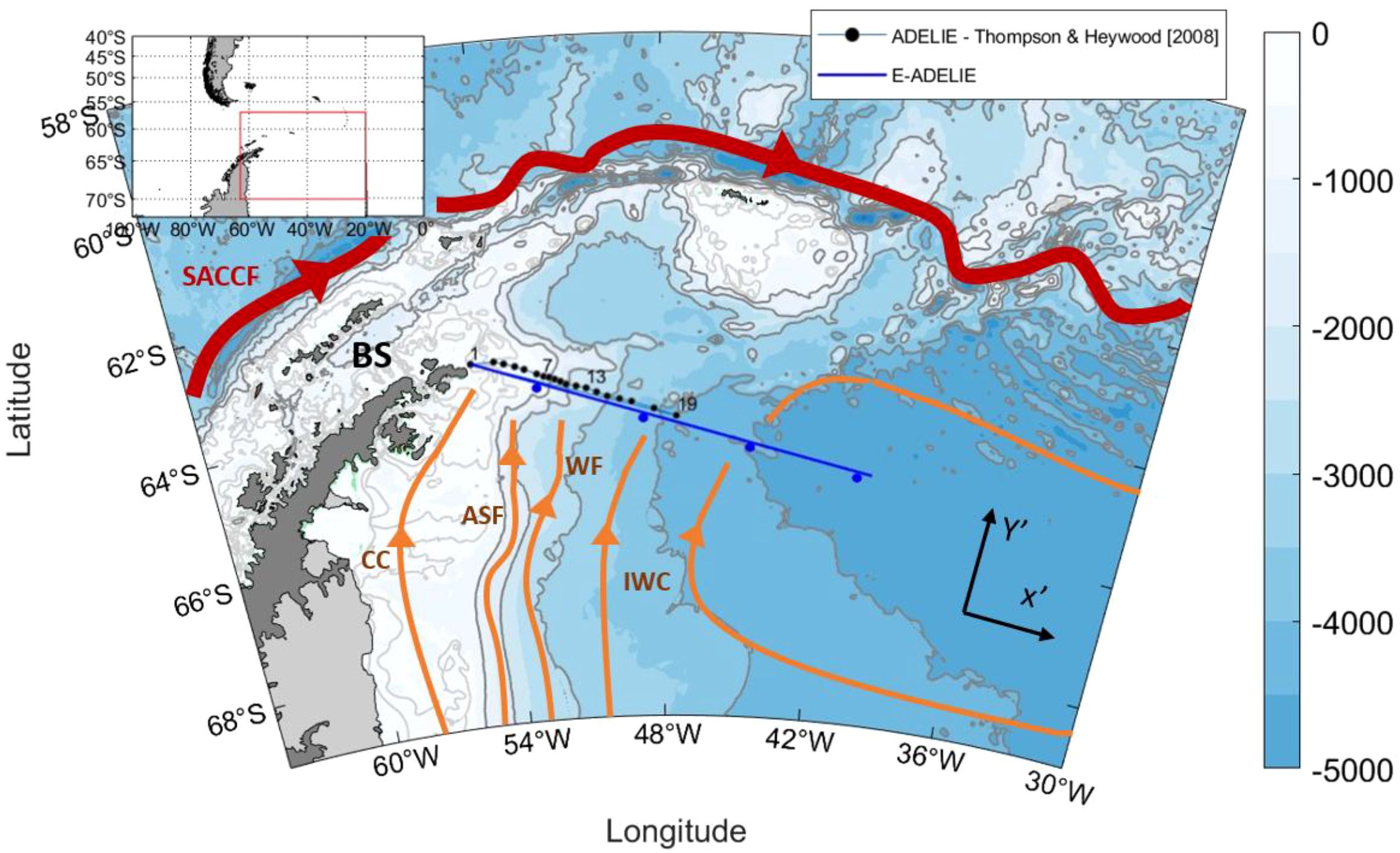
Figure 1. Bathymetric map of the northwestern sector of the Weddell Gyre depicting the study area with the approximate location of major oceanographic features and currents. Acronyms represent the Southern Antarctic Circumpolar Current Front (SACCF), Antarctic Coastal Current (CC), Antarctic Slope Front (ASF), Weddell Front (WF), Inner Weddell Current (IWC), and Bransfield Strait (BS). The ADELIE transect (Cruise 158 of RRS James Clark Ross in February 2007), as studied by Thompson and Heywood (2008), and the E-ADELIE transect are shown. ADELIE stations are marked with black dots and labelled with station numbers. The E-ADELIE transect is depicted in blue, with four blue dots indicating distances of 100, 300, 500, and 700 km from the coast to offshore. The new velocity field reference frame is displayed on the right. Fine light gray lines represent bathymetric contours at 200 and 400 m depth, while darker gray lines indicate depths of 1000, 2000, 3000, 4000, and 4500 m. The bathymetry originates from topo_8.2.img (Smith and Sandwell, 1997).

A particularly complex pattern of currents takes place along the Western Boundary Current System (WBCS) of the Weddell Sea. Over this domain, a multi-jet structure is present (Figure 1). Water masses flowing within the western branch of the gyre either recirculate within the gyre or leave the basin towards the Bransfield Strait or the Scotia Sea, and then flow northward into the South Atlantic Ocean (Naveira Garabato et al., 2002; Hellmer et al., 2005). These exported water masses change the Earth’s climate by redistributing the total heat and carbon content in the global ocean (Lumpkin and Speer, 2007; Styles et al., 2023; Talley et al., 2003; Vernet et al., 2019). Hence, if climate models and global ocean circulation reanalysis products do not resolve the Weddell Gyre circulation and converge towards aligned results, long-term projections could become divergent and lead to inconclusive future case scenarios.

In this work, we assess the baseline variability of the Weddell Gyre circulation along its western boundary, focusing on seasonal variability, to establish a foundation for future research exploring longer-term variability. The WBCS of the Weddell Sea presents three major bottom-intensified currents, corresponding to the Antarctic Coastal Current (CC), the Antarctic Slope Front (ASF), and the Weddell Front (WF) as shown in Figure 1 (Kerr et al., 2012; Stewart and Thompson, 2016; Thompson et al., 2018). The CC is primarily barotropic and drives the exit of Weddell waters towards the Bransfield Strait, allowing the leakage of near-freezing surface to subsurface waters (Morrison et al., 2023). In this manner, the CC forms a cold-water pathway which feeds the west Antarctic Peninsula and maintains regionally low rates of glacier retreat (Cook et al., 2016). Further offshore, the ASF is formed along the continental slope of Antarctica as a strong, narrow and persistent jet (Thompson and Heywood, 2008; Vernet et al., 2019). The ASF exhibits two northward-flowing cores, where the shoreward core is mainly barotropic, and the offshore core has a significant baroclinic component. Similarly, the WF core also shows an important baroclinic component, with velocities decreasing from the bottom to the surface (Thompson and Heywood, 2008).

Across the ASF, there is a rapid change in temperature and salinity mainly due to the interaction between two water masses: the colder and fresher waters of the Antarctic continental shelf, formed as a result of sea-ice formation and melting processes; and, the relatively warm and saline waters sourced by the Antarctic Circumpolar Current (ACC), entering the gyre from the eastern section (Thompson and Heywood, 2008; Vernet et al., 2019). The former water mass is known as Antarctic Surface Water (AASW), while the latter water mass is a modified Circumpolar Deep Water known as Warm Deep Water (WDW) within the Weddell Sea (Schröder and Fahrbach, 1999). Over the continental shelf, dense shelf water produced during sea-ice formation cascades down the continental slope and mixes with WDW. This process allows the dense water to reach the ocean bottom and continue its pathway through the global ocean. This dense bottom water is known as Antarctic Bottom Water (AABW), which originates from Weddell Sea Bottom Water (WSBW) and Weddell Sea Deep Water (WSDW) before exiting the Weddell Sea (Naveira Garabato et al., 2002; Llanillo et al., 2023; Muench and Gordon, 1995; Orsi et al., 1999; Stewart and Thompson, 2012).

Given its location, hydrographic structure, and dynamics, the ASF plays a crucial role in the exchange of heat, salt, and nutrients between the deep ocean and the Antarctic continental shelf waters, influencing the distribution of marine ecosystems and the dynamics of sea-ice formation and melting (Vernet et al., 2019). In this region, the melting of ice shelves is strongly influenced by the WDW (Cook et al., 2016). Beyond the north-western Weddell Sea, other regions of the gyre are also subject to oceanic forcing that influences sea-ice dynamics and glacier retreat. In particular, the eastern Weddell Gyre and the ice shelves along Dronning Maud Land are affected by the intrusion of relatively warm modified WDW, which can modulate basal melt rates (Mueller and Timmermann, 2018). However, the ASF is not entirely circumpolar; it is interrupted by the Antarctic Peninsula, separating the Pacific and Atlantic sectors of the Southern Ocean (Thompson et al., 2018). Specifically, it is absent along the West Antarctic Peninsula and large parts of the Bellingshausen Sea. Further oceanward, the WF is located as a major frontal system linked to high mesoscale variability in the form of eddies and meanders (Heywood et al., 2004; Thompson and Heywood, 2008). An overview of the water masses which compose the multi-jet structure of the WBCS in the reanalysis products as compared to observations is provided in the Supplementary Material, including their main characteristics (Figure A1 and Table A1-A2).

For a realistic simulation of ocean dynamics in high-latitude basins like the Weddell Sea, careful attention to horizontal resolution is essential (Neme et al., 2021; Renner et al., 2009). An idealized model study of the Weddell Gyre by Styles et al. (2023) explored how mesoscale eddies influence the Gyre’s transport and interaction with the ACC. The authors varied horizontal resolutions across eddy-parameterized (80 and 40 km), eddy-permitting (10 and 20 km), and eddy-rich (3 km) scales. They found that the strongest transport (45 Sv) occurred at eddy-permitting scales, which partially resolved large ocean eddies and enhanced thermal wind transport. The weakest transport (12 Sv) was at eddy-parameterized resolutions. Their recommendation to ocean modelers is to approach the eddy-permitting resolution with care when simulating the Southern Ocean and to consider employing parameterizations that are compatible with partially resolved mesoscale eddies. Styles et al. (2023) adopted a time-averaged forcing to produce the Weddell Gyre and ACC in their study, acknowledging that this idealized approach poses limitations, as the real ocean’s Weddell Gyre and ACC experience pronounced seasonal fluctuations. These fluctuations significantly alter the Gyre’s transport (Neme et al., 2021) and the density structure on its western boundary (Hattermann, 2018). However, estimates of the Weddell Gyre transport based on observations are constrained across seasons, particularly during winter, and exhibit considerable variability.

The scarcity of year-round estimates of the Weddell Gyre transport based on observations fuels the motivation behind this work. We use an open-access global ocean eddy-resolving reanalysis product and altimetry observations to investigate the seasonal variability of the Weddell Gyre circulation along its western boundary, building on previous observational and modelling works. The target is to characterize the key dynamical features of seasonal variations and assess the interplay of thermohaline gradients and wind stress forcing across seasonal scales. To this end, we select the historical transect known as ADELIE (Antarctic Drifter Experiment: Links to Isobaths and Ecosystems), which corresponds to western part of the SR04 WOCE section, as the study area. The ADELIE transect is depicted in Figure 1 and constitutes the most convenient reference frame to assess the ocean dynamics in the northwest of the Weddell Gyre. This location serves as a gateway for water masses sourced from the Weddell Sea, where they either exit the basin or recirculate within the gyre, potentially influencing downstream processes in the thermohaline circulation (Thompson and Heywood, 2008). Estimates of volume transport across this (or analogous) transects have been reported in the literature to range between 24–29 Sv, depending mainly on the season and the performed sampling strategy (Gordon et al., 2020; Muench and Gordon, 1995; Thompson and Heywood, 2008). However, in-situ observations reported in the literature are mostly representative of the free sea-ice seasons since the extreme meteorological conditions prevailing during the rest of the year prevent continuous observations. Also, remotely-sensed observations about the surface ocean dynamics are limited during the sea-ice seasons because the presence of the sea-ice cover poses a major challenge for satellite sampling. Hence, the use of reanalysis products becomes crucial so that the governing year-round ocean dynamics in this region can be explored without time gaps. Accordingly, we analyze the horizontal and vertical structure of the WBCS and its volume transport across an extended version of the historical ADELIE transect using a reanalysis product. We refer to this transect hereafter as the Extended ADELIE transect (E-ADELIE, Figure 1). This transect captures the full circulation across the western Weddell Gyre, extending from the northernmost tip of the Antarctic Peninsula oceanward through the WBCS into the Gyre’s interior.

The manuscript is structured as follows: Section 2 describes the data and methods. Section 3 presents the results and discussion, including the analysis of the horizontal and vertical structure of the WBCS using altimetry data and GLORYS12V1, the characterization of the seasonal cycle of volume transport, and an examination of the thermohaline and wind forcings driving this seasonality. Finally, Section 4 concludes the manuscript with a summary of the main findings.

2 Data and methods

In this section, we present the open-access reanalysis product analyzed in this study, along with its main configuration details. Next, we describe the altimetry and wind products used to complement our analyses. Lastly, we outline essential aspects of the methodology, including the rotation of the reference system, considerations for volume transport computations, the extrapolation technique used to fill data gaps over the continental slope while accounting for bottom-intensified jets, and the calculation of wind stress in an ocean influenced by sea-ice formation. For the seasonal analysis, we follow the criteria of Zhang et al. (2011) and Dotto et al. (2021) to define austral seasons as follows: summer (January–March), autumn (April–June), winter (July–September), and spring (October–December).

In the following, we use the term velocity field to refer to the combination of geostrophic and ageostrophic components. When only geostrophic balance is used in calculations, that velocity is simply referred to as the geostrophic velocity. Additionally, a variable accompanied by a prime indicates the rotated component (i.e., perpendicular to the transect or cross-transect component; see new reference frame in Figure 1). These conventions apply equally to both velocity and volume transport. Finally, the baroclinic and barotropic components are calculated as follows. The barotropic component is obtained by averaging the velocity profile over depth at each location, while the baroclinic component is derived by subtracting the barotropic component from the velocity profile at each location.

To investigate seasonal variability, we constructed a 12-point seasonal climatology based on monthly mean fields (January–December) averaged over the 1993–2020 period. This approach allows a higher temporal resolution than four broad seasonal means and enhances the robustness of correlation analyses. Throughout the manuscript, we use the term monthly exclusively in this context, not to analyze monthly variability per se, but to derive a resolved seasonal cycle. The mean state refers to the multi-year (1993–2020) climatological average, used as a reference or baseline for comparisons.

2.1 Data

We use GLORYS12V1, a global ocean eddy-resolving reanalysis product provided by the Copernicus Marine Environment Monitoring Service (CMEMS) and available at https://doi.org/10.48670/moi-00021. This product is based on the NEMO platform (Nucleus for European Modelling of the Ocean) and forms part of the Global Ocean Data Assimilation Experiment (GODAE) (Bell et al., 2009; Chassignet, 2011; Dombrowsky et al., 2009).

GLORYS12V1 is derived from the GLOBAL_REANALYSIS_PHY_001_030 product and is based on the NEMO 3.1 ocean model coupled with the LIM2 sea-ice model using the EVP rheology scheme. The system is forced by ECMWF atmospheric reanalyzes (ERA-Interim and ERA5), with corrections applied to shortwave and longwave radiation and precipitation. Vertical mixing is represented using a Turbulent Kinetic Energy (TKE) scheme with a fixed mixing length of 10 meters, and the model uses 50 vertical levels with a fixed vertical coordinate system. Surface salinity is restored using both 3D salinity profiles (from surface to bottom) and 2D sea surface salinity data. Sea-ice concentration is assimilated using data from both CERSAT and OSISAF sources. Regarding the horizontal resolution, it is 0.08°, approximately 5.4 km, which enables the resolution of mesoscale features globally, including at high latitudes. The bathymetry source is ETOPO1 for deep ocean regions and GEBCO8 for coastal and continental shelf areas. Moreover, the dataset provides daily-averaged outputs from January 1st, 1993 to June 1st, 2021. Key physical variables used in this study include potential temperature (°C), salinity (10⁻³), the meridional and zonal components of ocean velocity (v and u in m s^-1), sea-ice area fraction, and sea-ice thickness (m).

The surface circulation from GLORYS12V1 is compared to the geostrophic circulation in the study area, obtained from the altimetry product SEALEVEL_GLO_PHY_L4_MY_008_047, which is derived from multiple altimeter missions spanning 1993 to 2020. This data, processed by the DUACS system, has a spatial resolution of 0.25° and daily temporal coverage. Given the harsh winter conditions and extensive sea-ice cover in the Weddell Sea, traditional altimetry presents challenges. The altimetry product used accounts for sea-ice, flagging data when ice concentration exceeds 15%. To construct climatological surface velocity sections along the E-ADELIE transect, we set a threshold criterion requiring at least 70% data coverage per year for spring, summer, and autumn. This means that a minimum of 63 days of data per 90-day season is needed for the season of a given year to be included in the time-averaging process. However, to represent winter, this threshold must be reduced to 40% so that a handful of years enters into play in the time-averaging process. Once the seasonal average for all available years is calculated, we constructed the climatology for each season. By applying these thresholds, the following years are included in the seasonal averages that we present in this study: summer (29 years: 1993–2021 but 2015), autumn (8 years: 1993, 1999, 2000, 2002, 2006, 2009, 2011, 2021), winter (5 years: 2001, 2004, 2008, 2018, 2021) and spring (10 years: 1996, 2001, 2003, 2004, 2008, 2010, 2011, 2016, 2018, 2021).

This study employed the CMEMS altimetry product distributed between 2021 and November 2024. While this version is no longer available through the CMEMS catalogue, it was the official release at the time of data processing. Users accessing the CMEMS platform today may encounter a newer version: https://doi.org/10.48670/moi-00148. However, the product used here was previously validated in the study region and demonstrated to be suitable for mesoscale applications, as reported by Veny et al. (2025).

Finally, to keep consistency, the wind stress products used for further analyses in this study are the same as those used to force the GLORYS12V1 reanalysis. GLORYS12V1 uses ERA-Interim and ERA5 datasets. Since ERA-Interim was discontinued in 2019, ERA5 forcing fields have been applied starting from January 2019. In Figure 2, the area analyzed for correlations of volume transport across the E-ADELIE transect and basin-scale wind forcing is highlighted in red dashed lines.

Figure 2

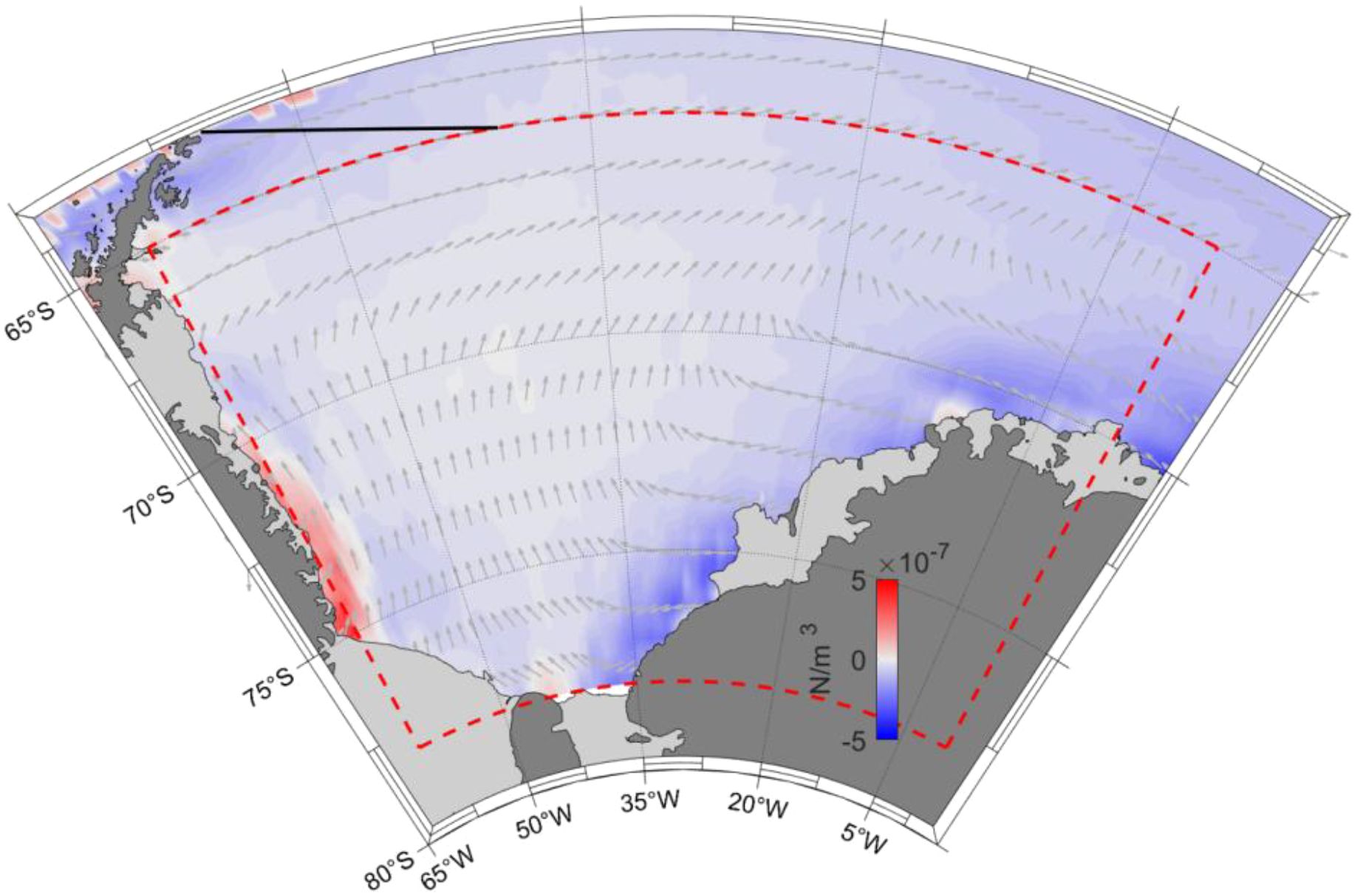
Figure 2. Horizontal map of the climatological wind stress (unit vectors) and wind stress curl (N/m³) over the Weddell Sea area between 1993 and 2020 (ERA-Interim and ERA5). The E-ADELIE transect is marked in black solid line. The area analyzed for correlations of volume transport across the E-ADELIE transect and basin-scale wind forcing is highlighted in red dashed lines.

2.2 Methods

For volume transport calculations, we compute the velocities perpendicular to E-ADELIE, denoted as lowercase v’. This procedure allows us to quantify the outflow of Weddell Sea waters across the E-ADELIE transect. The rotation angle is estimated from the average angle of the E-ADELIE transect with respect to the true east. Thus, the Cartesian coordinates were rotated 15.79 degrees clockwise from the true east. Subsequently, the rotated volume transport (uppercase V’), hereafter referred as the cross-ADELIE volume transport, is estimated daily from v’ at every time step of GLORYS12V1 (1993-2020) following Equation 1:

$\begin{array}{ll}{V}^{\prime }(t)= {\int }_0^{D_L} {\int }_{-h}^0 v^{\prime }(t)dzdx\text{'}& (1)\end{array}$

Here, 0 and DL denote the westernmost and easternmost integration limits, respectively. The values 0 and -h represent the integration depths, ranging from the surface at 0 m to the bottom, depending on the location. Finally, v’ refers to the time-dependent cross-ADELIE velocity component. The deepest bottom boundary for the integration is set at 4400 m because it corresponds with the last available depth provided by GLORYS12V1 in this region, even though one must note that the seafloor reaches depths down to 4800 m offshore E-ADELIE (~500 km). In all cases, the time-averaged and associated standard deviation of V’ are computed for the entire time coverage of GLORYS12V1 (1993-2020).

To account for bottom-intensified jets and ensure accurate volume transport calculations along the continental slope, we employed an extrapolation method to fill in data gaps near the sea-bottom. This method, available in MATLAB as inpaint_nans by D’Errico (2024) has been already tested and utilized successfully in Veny et al. (2022). The employed algorithm performs realistic extrapolation by considering the surrounding gradients to fill in data gaps. The function is applied in segments, taking pairs of stations to ensure its good performance and accurate results. A comparison of the mean V’ calculated between 1993–2020 for GLORYS12V1 along E-ADELIE, before and after applying the bottom extrapolation, shows an increase of about 4 Sv accounting for the data gaps along the continental slope.

We use Sea Surface Height (SSH) data provided by GLORYS12V1 to determine the geostrophic velocity at the surface, which will serve as our reference level. To assess the contribution of thermohaline gradients to the velocity field provided by GLORYS12V1, we separately calculate the geostrophic velocities considering only temperature gradients (with uniform salinity) and those due to salinity gradients (with uniform temperature). For both estimations, mean seasonal temperature and salinity fields have been used (accounting for four seasons during the 1993–2020 period).

We compute wind stress accounting for the drag coefficient values as a function of sea-ice concentration, as proposed by Lüpkes and Birnbaum (2005), following Equation 2:

$\begin{array}{ll}\tau = \rho · U_{10}^{ 2} · C_i& (2)\end{array}$

where ρ represents the air density (1.2 kg m^-3); $U_{10}=\sqrt{u_{10}^2+v_{10}^2}$ is the wind speed at 10 m above the surface (with $u_{10}^2$ and $v_{10}^2$ denoting the eastward and northward velocity components, respectively); and, C_i is the drag coefficient calculated following Lüpkes and Birnbaum (2005), which accounts for variations in sea-ice concentration by adjusting the surface roughness and momentum flux accordingly. For a full description of the formulation and parameter values, the reader is referred to Lüpkes and Birnbaum (2005). Wind stress curl is computed from the τ_x and τ_y components of the wind stress, accounting for sea-ice over the Weddell Sea. To assess the average wind patterns acting over the study area, basin-scale calculations are performed (see Figure 2). Finally, the relationship between the seasonal cycles of the wind forcing and volume transport driven by the WBCS is addressed through correlation analyses.

All reported ± values throughout this manuscript correspond to the standard deviation of the respective variable computed over the full time series. These values reflect the temporal variability of the dataset and are not formal estimates of statistical error.

Lastly, regarding the horizontal boundaries of each jet (CC, ASF, WF, and IWC), we note that there is no standardized method in the literature for their precise delimitation. In this study, we defined the lateral extents of each jet based on the spatial structure of surface and bottom velocity fields (see Figures 3b, d, 4b), identifying the points along the transect where velocity magnitudes consistently increase and then decrease. These transitions, interpreted as velocity gradients, were used to delineate the start and end of each jet. Our approach also considered the approximate positions reported by Thompson and Heywood (2008), ensuring consistency with previous work and allowing for a robust estimation of the spatial width of each current.

Figure 3

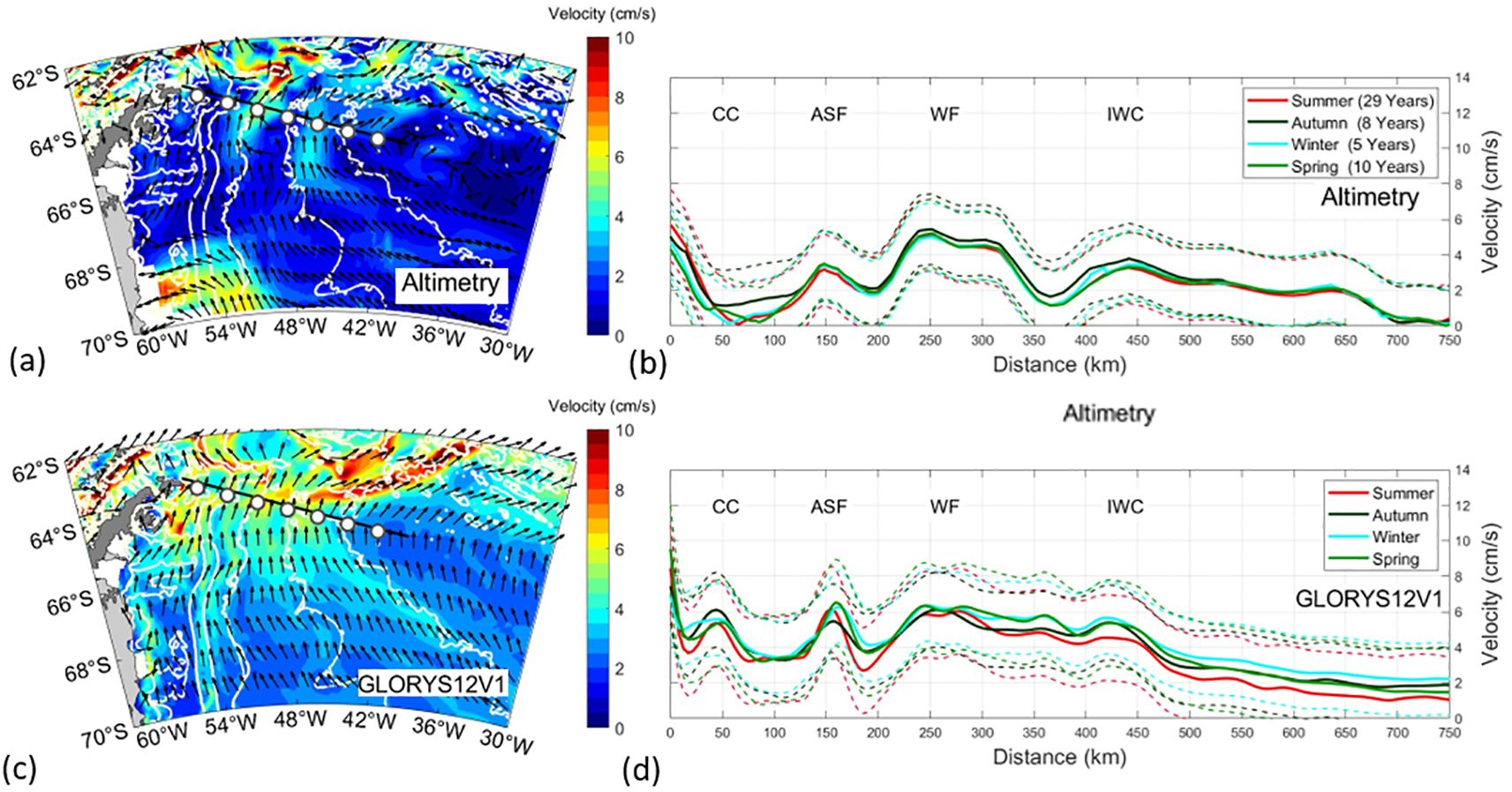
Figure 3. (a, c) present the horizontal structure of the WBCS in the Weddell Gyre. (a) shows time-averaged surface geostrophic velocities derived from altimetry data (2001, 2004, 2008, 2018, 2021), whereas (c) shows time-averaged surface velocities from GLORYS12V1 (1993-2020). The flow direction is indicated with unit vectors. The E-ADELIE transect is indicated by a black line, with white dots marking every 100 km between 0 and 750 km along the x-axis of (b, d). Fine white lines trace bathymetric contours at 200 and 400 m depth, while thicker white lines correspond to depths of 1000, 2000, 3000, 4000, and 4500 m. (b) shows the seasonal surface geostrophic velocity (cm/s) along E-ADELIE and computed from altimetry data (1993-2020; see section 2.1 for the years corresponding to each season). (d) is analogous to (b), but it shows the seasonal surface velocity (cm/s) computed from GLORYS12V1 data (1993-2020). The dashed lines indicate the seasonal mean value ± the standard deviation.

Figure 4

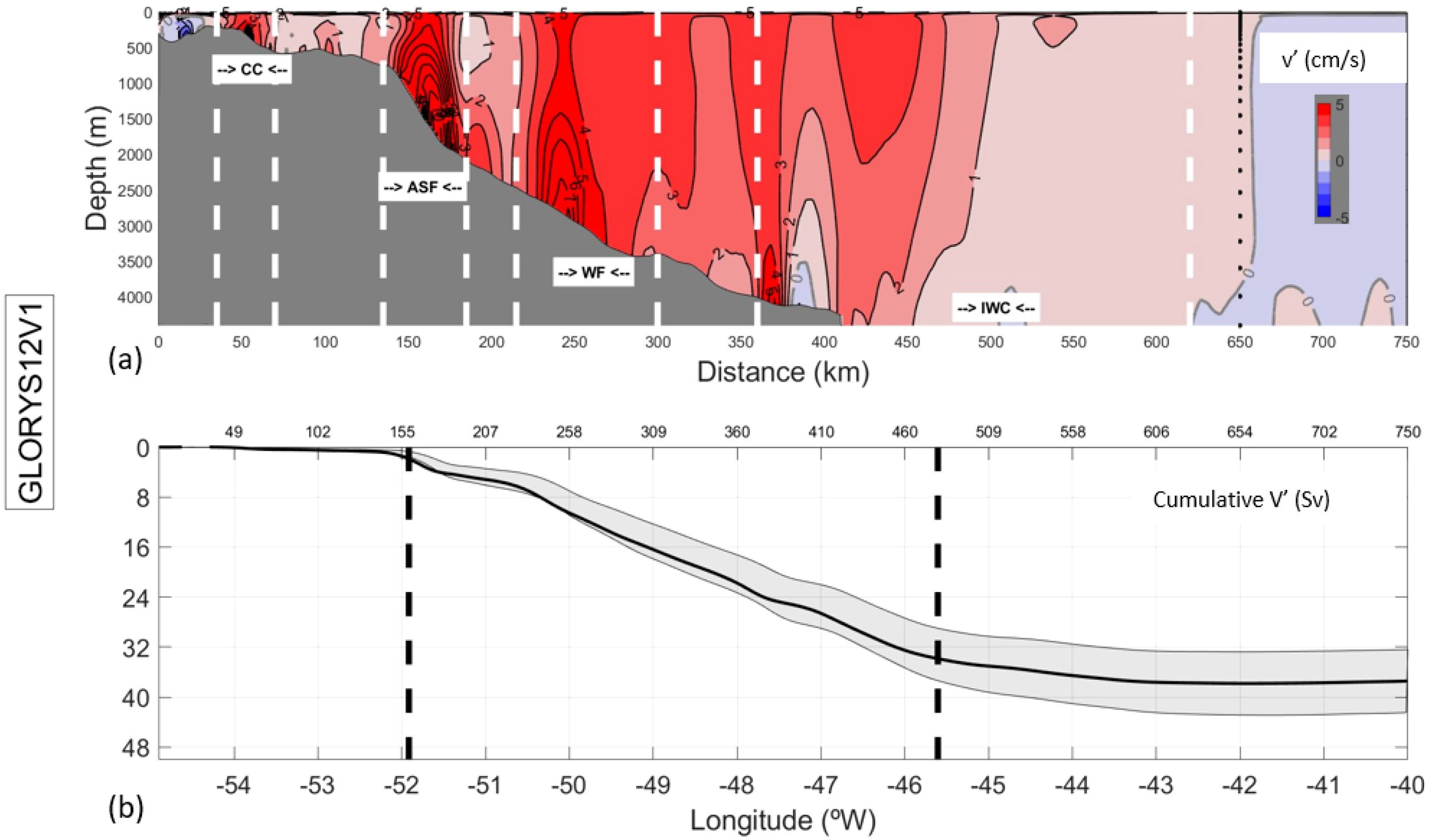
Figure 4. (a) Time-averaged velocity field of v′ (cm/s) along the E-ADELIE transect. (b) Cumulative transport V′ (Sv) of the time-averaged velocity field v′ along E-ADELIE. The time average corresponds to the period from 1993 to 2020. Dashed black lines are used as reference locations for discussing the results in the text. Black dots at 650 km offshore indicate the vertical resolution of the GLORYS12V1 output. The position of the fronts is defined following the white dashed lines and their acronyms, corresponding to: Coastal Current (CC), Antarctic Slope Front (ASF), Weddell Front (WF), Inner Weddell Current (IWC).

3 Results and discussion

The applicability of Sverdrup dynamics for calculating the Weddell Gyre transport is not straightforward and has been questioned for decades, as in Gordon et al. (1981), where its transport was estimated to be ~76 Sv using wind stress data and applying Sverdrup balance. Subsequent studies using moorings and ship data have provided lower estimates with larger ranges: 20–56 Sv in Fahrbach et al. (1991) and about 30 Sv in Yaremchuk et al. (1998). A review of the existing literature identifies several papers that have addressed the Weddell Gyre transport using idealized models, reanalysis products, and observations, as listed in Table 1 (see section 3.2). Beyond these full-depth transport estimates, some studies have focused on the export of WSBW (a component of AABW, along with WSDW). Gordon et al. (2010) identified a seasonal cycle in the export of WSBW southeast of the South Orkney Islands, with variability linked to wind forcing over the western Weddell Sea. Fahrbach et al. (2001) estimated an average bottom water transport of 1.3 ± 0.4 Sv in the northwestern Weddell Sea, with fluctuations on both annual and interannual timescales. More recently, Llanillo et al. (2023) provided updated estimates of WSBW transport, reporting annual-mean values of 3.4 ± 1.5 Sv, further illustrating the long-term variability in deep water export.

Table 1

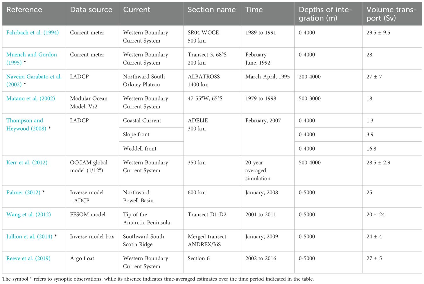
Table 1. Review of volume transport estimates computed across transects analogous to ADELIE, based on both observational and model data.

In the next sections, we assess the seasonal variations of the WBCS of the Weddell Gyre, building on the framework established in the literature, using an open-access global ocean circulation reanalysis product (GLORYS12V1) and altimetry data.

3.1 Horizontal structure

We present the climatological spatial structure of the WBCS of the Weddell Gyre at the surface, based on the time-averaged velocity field from altimetry data (2001, 2004, 2008, 2018, 2021) and GLORYS12V1 output (1993–2020). These results are shown in Figure 3a, c (upper and lower panels, respectively).

The most prominent feature derived from altimetry data (geostrophic velocity field) and GLORYS12V1 output (velocity field) is the multi-jet structure of the WBCS. This structure consists of a series of parallel-aligned jets (CC, ASF, WF) and a broad current running nearly perpendicular to the transect E-ADELIE, departing from the Antarctic Peninsula’s tip and extending oceanward (Figure 3). The latter current is a previously unreported feature of the Weddell Gyre’s circulation, described extensively for the first time in this study, which we refer to as the Inner Weddell Current (IWC). This multi-jet structure is in good agreement with studies based on in-situ observations (Muench and Gordon, 1995; Thompson and Heywood, 2008) and modelling studies (Stewart and Thompson, 2016; Matano et al., 2002). In this study, GLORYS12V1 output and altimetry data present the ASF centered at ~150 km, and the WF centered at ~260 km, from the coastline to offshore distances, with a width approaching 100 km in all cases (Figure 3). These locations are in agreement with those reported in Thompson and Heywood (2008), and derived from Shipborne Acoustic Doppler Current Profiler (SADCP) and Lowered Acoustic Doppler Current Profiler (LADCP) measurements, supporting the good performance of both products. This is further reinforced by recent validation efforts of these products conducted in nearby regions with similarly challenging conditions due to sea-ice and limited in-situ data (Artana et al., 2017; Damini et al., 2025; Ferrari et al., 2017; Frey et al., 2021, 2023; Veny et al., 2025).

The individual jets are clearly identified in the surface velocity sections sampled along E-ADELIE (Figure 3b, d). Notably, the CC appears as a distinct coastal flow only in the GLORYS12V1 output, with increasing magnitude near the shore. In contrast, it is absent in the altimetry data, likely due to the influence of land proximity. Maximum mean climatological speeds for each jet, derived from altimetry data and GLORYS12V1 output (Figure 3), are consistent and of the same order of magnitude: 4 cm/s for the ASF and 6 cm/s for the WF in altimetry data, and 6 cm/s for both jets in GLORYS12V1. As expected from time-averaging, these values are generally lower than synoptic SADCP and LADCP measurements reported by Thompson and Heywood (2008), which indicate 20 cm/s for the ASF and 10 cm/s for the WF. Additionally, the IWC stands out as a distinct broad current in altimetry data, flowing northeastward as a part of the inner core of the Weddell Gyre, where interior waters recirculate. The presence of the IWC is confirmed year-round, as it appears in the seasonal surface geostrophic velocity sections shown in Figure 3b. Although less prominent, the IWC is also visible in the seasonal surface velocity sections shown in Figure 3d. This current is observed between 350 km and 620 km offshore the Antarctic Peninsula in altimetry data and GLORYS12V1 output, reaching maximum seasonal mean values between 4 to 6 cm/s, respectively (Figure 3b, d). The presence of these jets across all seasons and its consistent positioning suggest that, despite the uneven seasonal coverage of SSH data (29 years of summer data compared to only 5 years of winter data), these observations can be considered representative of all seasons for the purposes of this study.

Generally, the weaker strength of the modelled jets as compared to observations can be attributed to two factors. First, the SADCP and LADCP data reflect synoptic measurements, while the GLORYS12V1 output presented here are time-averaged climatological values, which tend to be smoother. Second, reanalysis products assimilate remotely-sensed data, including scatterometer and altimetry measurements, which often underestimate direct velocity measurements by 4-64%, as reported in Hart-Davis et al. (2018). This assimilation process may contribute to the underestimation of velocities, particularly in boundary currents, where altimetry-derived geostrophic velocities often fail to capture the full intensity of the flow (Hewitt et al., 2020). Lastly, the GLORYS12V1’s resolution (1/12°) limits its ability to resolve mesoscale and submesoscale dynamics, markedly in polar boundary current systems, leading to weaker eddy kinetic energy and underestimated velocity magnitudes.

3.2 Vertical structure and cumulative volume transport

The vertical structure of the WBCS is depicted in Figure 4 through time-averaged vertical sections of the rotated velocity field (v’) and cumulative transport (V’) along E-ADELIE, based on GLORYS12V1 data. The vertical distribution of v’ (Figure 4a) reveals a multi-jet structure characterized by bottom-intensified flows, including three distinct jets (CC, ASF, WF) and a broader current (IWC) extending toward the gyre’s interior. This structure is consistent with previous observations from the surface analysis of altimetry data and GLORYS12V1 output (Figure 3). The oceanward distribution of the cumulative transport per km, V’, within E-ADELIE shows a marked increase in transport values between a distance of 150 km and 470 km offshore; this domain is bounded by vertical dashed black lines in Figure 4b. The observed increase is nearly linear, with transport values of approximately 0.08 Sv per km. By performing an analogous analysis over the direct velocity measurements from Thompson and Heywood (2008), we find a higher rate of cumulative volume transport increase, at 0.11 Sv per km (based on transport estimates in their Figure 11). We attribute the lower cumulative transport rate in the GLORYS12V1 output to the influence of the reanalysis product’s horizontal resolution on resolving the mesoscale structure and associated high eddy kinetic energy of the WBCS, as discussed in the introduction. Beyond the offshore distance of 470 km, where the linear increase in cumulative volume transport weakens, the cumulative transport remains nearly constant at around 36 Sv.

When computing the cross-transect volume transport from the surface down to 4400 m depth over the IWC domain, spanning from about 50 km east of the Weddell Front and up to 620 km offshore from the Antarctic Peninsula, we obtain 16.2 ± 3.0 Sv in GLORYS12V1 output. This indicates that the IWC drives around 43% of the volume transport driven by the WBCS along the E-ADELIE section (37.3 ± 5.0 Sv), hence becoming the primary contributor to the transport of Weddell-sourced waters across the section.

3.3 Volume transport across seasonal scales

In this section, we analyze the seasonal variations of the full-depth volume transport captured in GLORYS12V1 output across the E-ADELIE transect. To this aim, we compute volume transport estimates following the methodology and assumptions detailed in section 2 (see Equation 1). Accordingly, GLORYS12V1 output provides a time-averaged (1993-2020) volume transport estimate of V’ = 37.3 ± 5.0 Sv. The comparison between the total volume transport (37.3 ± 5.0 Sv) and the estimate considering only northward flow (positive values, 37.9 ± 5.0 Sv) reveals a difference of less than 1 Sv. This suggests that the southward flow in this region is nearly negligible compared to the northward transport. In Figure 5, we present the seasonal cycle of the volume transport driven by the WBCS in the Weddell Sea through a series of monthly climatological estimates (see section 2): (a) full-depth cross-transect volume transport (V’) derived from GLORYS12V1 output, including a set of previously reported estimates of volume transport following the literature review presented in Table 1; (b) surface (0–100 m) cross-transect volume transport (V’) and Weddell Sea Bottom Water volume transport (V’) derived from GLORYS12V1 output and delimited using the threshold value of neutral density (γ_n) ≥ 28.4 kg/m³, as reported in the bibliography (Thompson and Heywood, 2008); and, (c) basin-scale wind stress and wind stress curl.

Figure 5

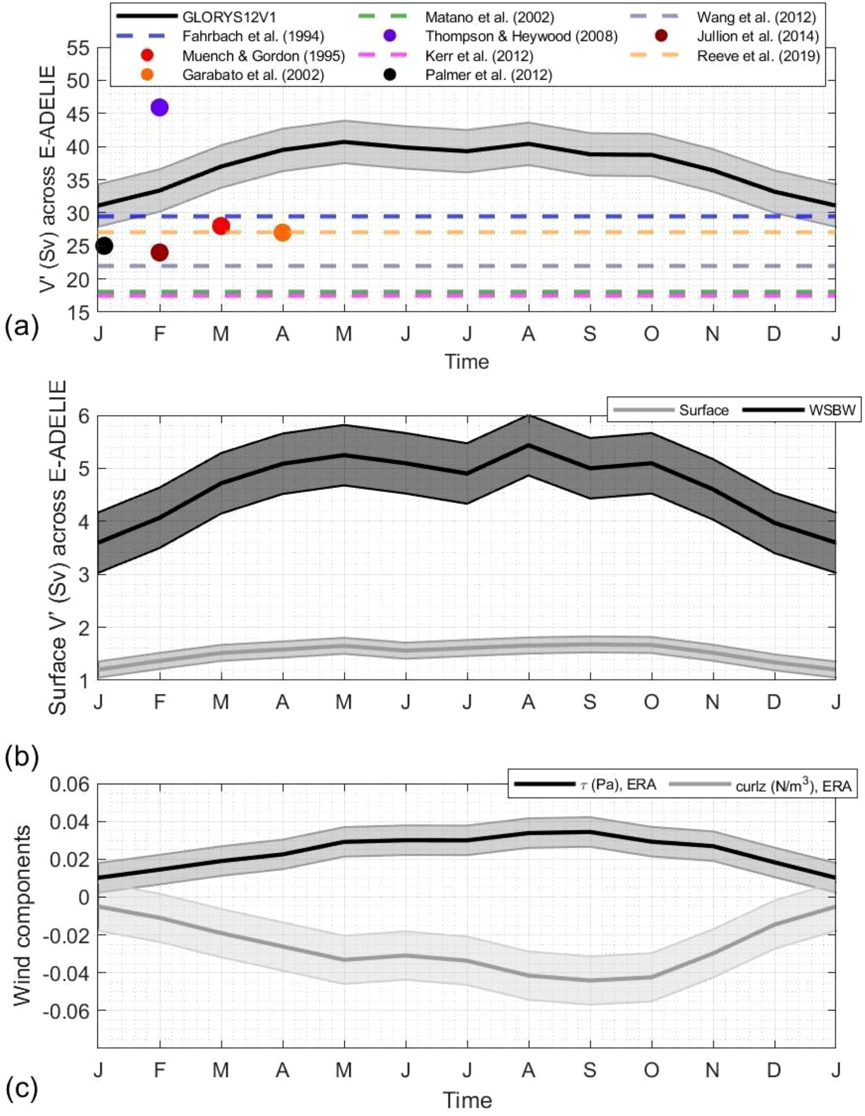
Figure 5. (a) Wind stress (τ) and volume transport (V′), across the E-ADELIE transect with their corresponding standard deviations (shaded areas around the climatological values). Observational data for transects analogous to E-ADELIE, as reported in the literature and listed in Table 1, are plotted as colored dots for synoptic-scale measurements and as horizontal dashed lines for time-averaged estimates. (b) Same as (a), but computed for the WSBW (γ_n ≥ 28.4 kg/m³) in black, and for the surface layer (0–100 m depth) in grey. (c) Basin-scale seasonal cycles of wind stress (black) and wind stress curl (grey) in Pa and N/m³, respectively. The wind stress curl is multiplied by 10⁶ for plotting purposes to match the range of the wind stress. The area under consideration is depicted in Figure 2.

The seasonal cycle of V’ peaks at 39.5 ± 0.8 Sv during winter and 40 ± 0.6 Sv in autumn, while the minimum values occur in summer at 33.8 ± 3.0 Sv, followed by spring values of 36.1 ± 2.8 Sv (Figure 5a). This seasonal variation results in a maximum seasonal amplitude of approximately 10 Sv. In Figure 5a, volume transport estimates previously reported in the literature (observational and modelling studies) are depicted as dots for synoptic values and as dashed lines for time-averaged values. At this point, it is worthwhile noting that formerly reported estimates represent full-depth integrated volume transports computed across transects similar to E-ADELIE. Notably, these estimates are generally consistent with model-based estimates from GLORYS12V1 output, particularly during summer and early autumn, when weather conditions in the study area are less extreme, and more observational data for assimilation purposes are available. The largest difference is observed in the time-averaged modelling-based estimates reported by Matano et al. (2002) and Kerr et al. (2012) summarized in Table 1; Figure 5a. These studies reported significantly lower volume transport values than the seasonal climatological estimates derived from GLORYS12V1 output (Figure 5a). Overall, comparisons with observational and modelling-based estimates in the literature suggest a realistic performance of GLORYS12V1. Furthermore, GLORYS12V1 has been validated in other studies, such as Lellouche et al. (2021), which demonstrated its robust performance globally and specifically within the Antarctic region.

Regarding the surface volume transport (Figure 5b), this reaches its highest levels during autumn and winter, peaking in May, August, and October at 1.65, 1.66, and 1.67 Sv, respectively, while its lowest level occurs in summer (January) at 1.20 Sv. Similarly, WSBW transport exhibits three distinct peaks from autumn to winter, with the highest values in May, August, and October (5.25, 5.44, and 5.01 Sv, respectively) and a minimum in summer (January) at 3.60 Sv. These results align with observations reported in Llanillo et al. (2023), who reported a peak in mid-autumn at 4.65 Sv and a minimum in mid-summer at 2.80 Sv.

A comparison of the seasonality of V’, surface V’, and WSBW V’ with the seasonality of wind stress, averaged spatially over the study area using ERA-Interim and ERA5 wind datasets, reveals a predominantly consistent pattern across the three panels (Figure 5c). This observation motivates a more detailed examination in the following section of the role of wind stress in driving the meridional transport of the WBCS, as captured by GLORYS12V1 in this region.

3.4 Interplay of thermohaline gradients and wind stress forcing

The dynamics governing the WBCS in the Weddell Gyre are shaped by a complex interplay of thermohaline gradients and wind stress forcing. These driving forces vary across spatial and temporal scales, influencing the development and intensity of the jets within the WBCS.

In the northern Weddell Sea, between approximately 50°S and 60°S, westerly winds dominate, while easterlies prevail south of 65°S. This wind pattern plays a crucial role in shaping the region’s ocean circulation, including the formation and dynamics of the Weddell Gyre. The strength of these winds varies seasonally, with a significant weakening during the austral summer, reducing wind-driven currents by nearly 50% compared to their winter and fall intensities (Armitage et al., 2018; Talley et al., 2011; Schröder and Fahrbach, 1999).

Figure 5 highlights the similarity between the seasonal cycles of cross-transect volume transport (V’), surface volume transport and WSBW volume transport, with the seasonal pattern of both wind stress and wind stress curl averaged over the study area. To assess this relationship in the Weddell Sea based on GLORYS12V1 output, we analyzed the correlations between the volume transport components (Figure 5a, b) and both wind stress and wind stress curl (Figure 5c). The results, presented in Table 2, demonstrate strong and statistically significant correlations between the surface, full-depth and bottom volume transport driven over the domain of the WBCS of the Weddell Sea, and both the wind stress and wind stress curl, with R² values ranging from 0.7 to 0.9. These findings are consistent with the theoretical framework of a wind-driven gyre modulated by the seasonal variability of wind stress curl (Azaneu et al., 2017; Franco et al., 2007; Von Gyldenfeldt et al., 2002; Le Paih et al., 2020; Wang et al., 2012). Existing analyses of the wind stress forcing in the WBCS have focused primarily on observations and modelling of the bottom water volume transport (Llanillo et al., 2023; Wang et al., 2012). However, to the best of our knowledge, this is the first time that an open-access global ocean reanalysis product has been assessed over the WBCS of the Weddell Sea to this aim, opening avenues to further explore the influence of wind stress forcing on each element of the multi-jet structure of this current system.

Table 2

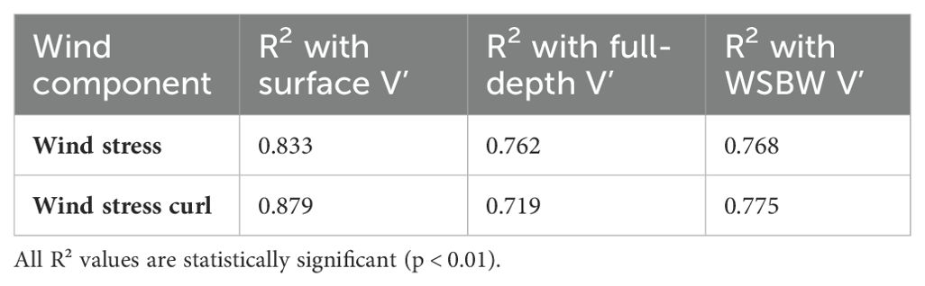
Table 2. R² values from linear regression models investigating the relationship between the seasonal wind stress and wind stress curl, and the seasonal cross-transect components of the surface (1–100 m), full-depth and Weddell Sea Bottom Water (WSBW) volume transports.

Expanding upon the theoretical framework of wind-driven gyres—where a single, fast-flowing western boundary current is typically expected—, we performed correlation analyses between the basin-wide wind stress forcing (see the forcing area in Figure 2) and the volume transport driven by each jet (see the domain for each jet in Figure 4). This analysis allowed us to assess whether wind forcing uniformly controls the temporal variability of the entire multi-jet system, or if different drivers influence each jet individually. The results reveal an oceanward increase in R², where the CC, ASF, and WF exhibited R² values of 0.3, 0.3, and 0.5, respectively, while the IWC reached an R² of 0.8. These findings indicate that wind stress forcing has a more significant influence on the IWC compared to the CC, ASF, and WF. Flowing away from the continental slope and, hence, less influenced by topographic steering, the IWC lacks an apparent thermohaline front, unlike the ASF and the WF (Figure 6).

Figure 6

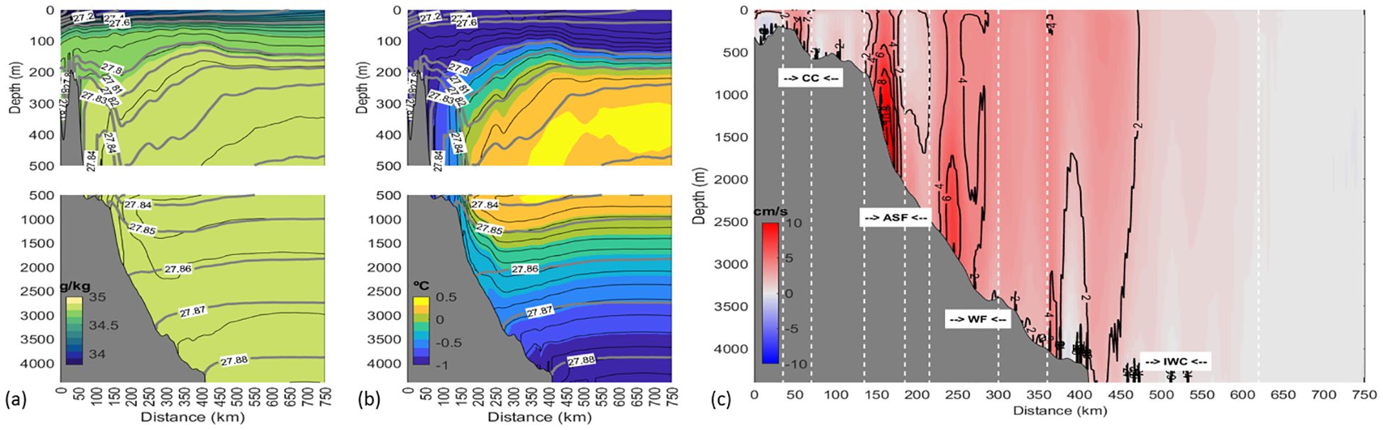
Figure 6. Vertical sections along the E-ADELIE transect showing (a) Absolute Salinity (g/kg), (b) Conservative Temperature (°C), and (c) geostrophic velocity (gv’, cm/s) under mean conditions (1993–2020) as represented in the GLORYS12V1 product. In (a) and (b), isopycnals are shown in gray with their respective values. In (a), isohalines (black contours) are plotted at 0.05 g/kg intervals from 0 to 500 m and at 0.01 g/kg intervals from 500 m to the bottom, without labels. In (b), isotherms (black contours) are plotted at 0.2°C intervals from 0 to 500 m and at 0.1°C intervals from 500 m to the bottom, without labels. In (c), gv’ contours are labeled with their respective values. The positions of the main currents and fronts are indicated by white dashed lines, with acronyms representing the Coastal Current (CC), the Antarctic Slope Front (ASF), the Weddell Front (WF), and the Inner Weddell Current (IWC).

In line with the increasing oceanward R² between the basin-wide wind stress forcing and the volume transport driven by each jet, we also find that the barotropic component of each jet is the predominant contributor—and in some cases, the only one—to the high correlation observed between the wind forcing and the volume transport in Table 2. Table 3 shows that the barotropic component exhibits R² values of approximately 0.4 for the CC, ASF, and WF jets, and values exceeding 0.7 for the IWC.

Table 3

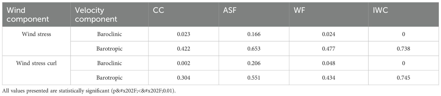
Table 3. R² values from linear regression models investigating the relationship between the seasonal wind stress (curl) and the seasonal cross-transect volume transport, V′, attributed to the baroclinic and barotropic velocity components for each jet (CC, ASF, WF, IWC) in GLORYS12V1.

The seasonal intensification of the baroclinic component of the WBCS, particularly across the ASF and WF, reflects the development of steep lateral density gradients during winter and early spring. These gradients strengthen during the period of sea-ice formation, when brine rejection in coastal polynyas increases shelf salinity and density, enhancing stratification near the slope (Tamura et al., 2008). This buoyancy forcing coincides with the seasonal eddy-driven upwelling and shoaling of isopycnals along the continental slope, which promotes onshore intrusions of warm, salty Circumpolar Deep Water (CDW) that enhance the thermal component of the density gradients (Stewart and Thompson, 2016; Thompson et al., 2018). The combined effect results in the formation of a V-shaped frontal structure (present in Figure 6a, b and Figure A1 for in-situ measurements (a, b) and for GLORYS (c, d))—a defining feature of the Dense Shelf regime described by Thompson et al. (2018)—that supports baroclinic shear and intensified geostrophic transport along the ASF. While the barotropic component, driven primarily by wind forcing (Table 3), dominates at shorter (monthly and intraseasonal) time scales, it interacts with the background stratification and bathymetry to modulate the vertical shear and structure of baroclinic jets. Overall, the emergence of a baroclinic circulation is fundamentally linked to these seasonal-scale processes involving buoyancy forcing, eddy activity, and topographic steering. Our results are thus consistent with the dynamical framework proposed for ASF systems where dense shelf water formation drives the seasonal evolution of the baroclinic structure (Thompson et al., 2018, their Figures 3b, e, 4c).

As discussed by Thompson and Heywood (2008), these jets are primarily geostrophic. This is evident from the comparison of Figures 4a, 6c, where the time-averaged velocity and geostrophic velocity fields are shown to resemble each other. Based on their geostrophic nature, Figure 7 independently evaluates the contributions of temperature and salinity gradients to the geostrophic velocity for each season. This is done by performing calculations where either only the temperature (left-hand side panels) or only the salinity gradients (right-hand side panels) are considered. This approach has been followed in previous studies to examine the relative dominance of each player in driving geostrophic flows (Batteen and Huang, 1998; Menezes et al., 2013). The color coding is interpreted as follows: red shades indicate areas where the geostrophic field computed using temperature (or salinity) data alone flows in the same direction as the overall multi-jet (northeastward), whereas blue shades indicate areas where it flows in the opposite direction (southwestward). Spatial variability is evident, particularly over the bottom-intensified cores of the ASF and WF, where temperature gradients strongly contribute to northeastward flows, while salinity gradients produce weaker northeastward flows (over the WF) and even reversed flows (over the ASF). In contrast, within the IWC region, both temperature and salinity gradients appear to support northeastward flows.

Figure 7

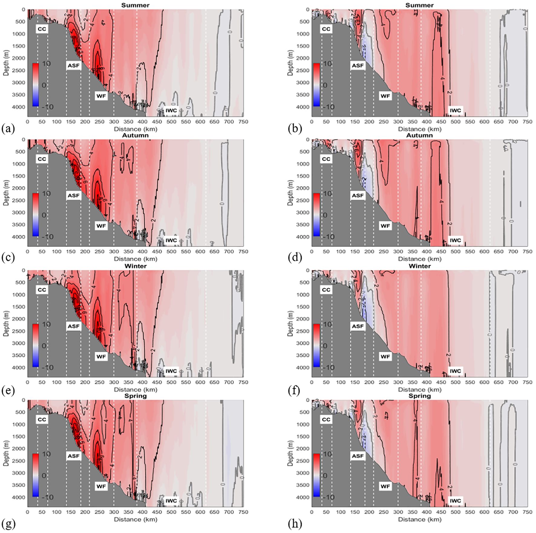
Figure 7. Seasonal geostrophic velocity field (gv, cm/s) along the E-ADELIE transect, for two scenarios. Left-hand panels (a, c, e, g) show geostrophic velocities computed with temperature gradients only (uniform salinity field). Right-hand panels (b, d, f, h) show geostrophic velocities computed with salinity gradients only (uniform temperature field). Rows correspond to: summer (a, b), autumn (c, d), winter (e, f), and spring (g, h), respectively (from top to bottom). The position of the jets is defined following the white dashed lines and their acronyms, corresponding to: Coastal Current (CC), Antarctic Slope Front (ASF), Weddell Front (WF), Inner Weddell Current (IWC).

These behaviors are further clarified in Figure 6. In the upper ocean, the isohalines overlap the isopycnals more closely than the isotherms, supporting that salinity gradients dominate the geostrophic flows in polar regions. However, at depth, neither the isohalines nor the isotherms are preferentially aligned with the isopycnals over the continental slope. This suggests that the bottom-intensified cores of the ASF and WF result from the combined effects of both temperature and salinity gradients, with temperature playing the dominant role in directing the flow (see Figure 7). Conversely, away from the slope and within the IWC domain (Figure 6), both the isohalines and isotherms mirror the pattern of the isopycnals, indicating a combined contribution to the flow direction, as supported by the calculations in Figure 7.

Although seasonal differences are not evident in Figure 7 over the domain of the bottom-intensified cores of the ASF and WF, some variability could reasonably be expected given that these jets are strongly linked to deep water formation and the sinking of dense waters following winter sea-ice formation (Llanillo et al., 2023; Wang et al., 2012). These differences become more pronounced in Figure 8 when the geostrophic field computed using both temperature and salinity contributions is subtracted from each seasonal field computed using only temperature and salinity gradients. Generally, salinity-driven geostrophic flows more strongly counteract the overall flow driven by temperature over the bottom-intensified cores of the ASF and WF, and the temperature-driven geostrophic flows are also stronger in winter. These observations are consistent with the steeper temperature and salinity gradients in the upper ocean after the sea-ice formation season (beginning in autumn) and the subsequent sinking of dense water down the continental slope. In summer, both temperature and salinity gradients relax, and the bottom-intensified cores of the ASF and WF appear embedded within a joint, weaker and broader core.

Figure 8

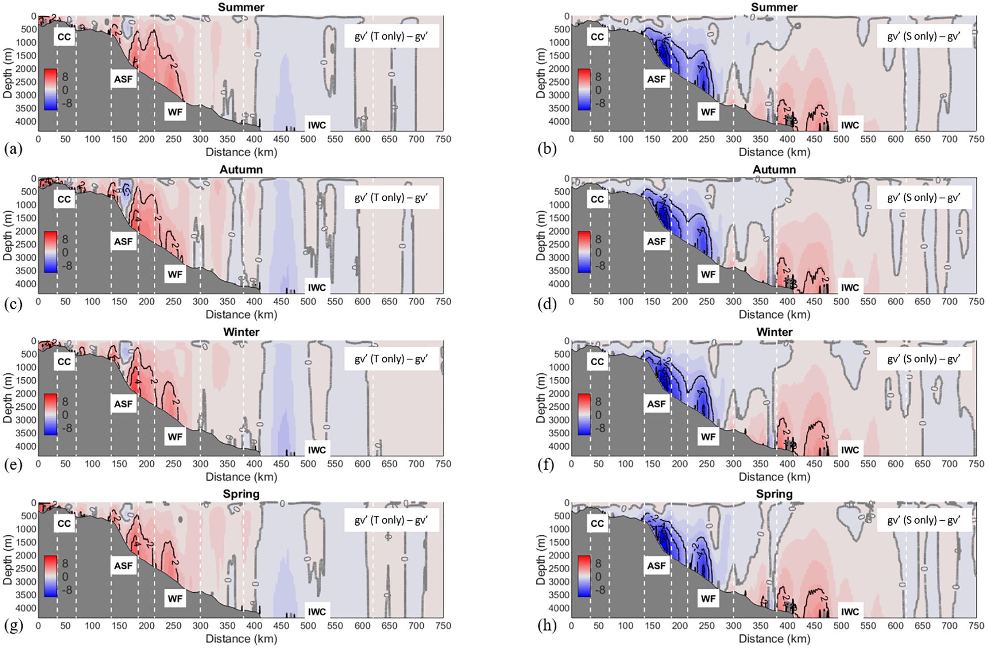
Figure 8. Seasonal geostrophic fields (gv’, cm/s) along the E-ADELIE transect assessing temperature and salinity contributions relative to the full geostrophic field. Left-hand panels show fields based solely on temperature, and right-hand panels show fields based solely on salinity, after subtracting the corresponding full geostrophic field computed with both temperature and salinity contributions. Rows represent summer, autumn, winter, and spring (from top to bottom). The position of the jets is defined following the white dashed lines and their acronyms, corresponding to: Coastal Current (CC), Antarctic Slope Front (ASF), Weddell Front (WF), Inner Weddell Current (IWC).

Results from this section indicate that the ASF and WF are primarily governed by geostrophic dynamics, with thermohaline gradients playing a crucial role in driving the core of the bottom-intensified jets—consistent with their association with steep density fronts over the continental slope (Thompson and Heywood, 2008; Thompson et al., 2018). However, additions are made to previous knowledge, as the dominant thermohaline influence varies with season and depth. This builds on previous studies reporting that the position and strength of the ASF are also, to some extent, sensitive to wind stress forcing on seasonal and interannual timescales (Su et al., 2014; Youngs et al., 2015; Meijers et al., 2016), as it remains an integral part of the western branch of a wind-driven ocean gyre. In contrast, the IWC appears to be driven mainly by wind stress forcing, as it lacks a distinct thermohaline front, likely due to its offshore location where step density gradients over the slope due to water mass formation are absent and topographic steering is less significant. These findings underscore the importance of seasonally- and depth-dependent analyses for understanding the interplay between thermohaline gradients and wind stress forcing in shaping the WBCS dynamics of the Weddell Sea, providing a comprehensive framework for predicting future circulation scenarios.

4 Conclusions

This study provides a comprehensive analysis of the seasonal variability and driving mechanisms of the Western Boundary Current System (WBCS) in the Weddell Gyre, using high-resolution data from the eddy-resolving global ocean reanalysis GLORYS12V1 and altimetry observations. The results confirm the persistent multi-jet structure of the WBCS, consisting of the Antarctic Coastal Current (CC), Antarctic Slope Front (ASF), Weddell Front (WF), and the newly identified Inner Weddell Current (IWC). The IWC emerges as a significant wind-driven feature, contributing approximately 43% of the total volume transport across the E-ADELIE transect (16.2 ± 3.0 Sv out of 37.3 ± 5.0 Sv), highlighting its key role in the recirculation of interior waters within the Weddell Gyre.

The seasonal variability of the WBCS is strongly modulated by wind stress curl, with maximum transport occurring in autumn (40 ± 0.6 Sv) and minimum values in summer (33.8 ± 3.0 Sv). Correlation analyses reveal a dominant influence of wind forcing on the IWC (R² ~0.8), while the CC, ASF, and WF exhibit weaker correlations (R² = 0.3, 0.3, and 0.5, respectively), indicating a lower dependence on wind forcing. Complementarily, thermohaline gradients are found to be particularly important over the continental slope, shaping the ocean dynamics of the ASF and WF through steep density fronts. In the upper ocean, salinity gradients control the density field, strongly influenced by sea-ice formation and melting processes. However, at depth, temperature gradients steer the northeastward-flowing geostrophic flow within the bottom-intensified cores of the ASF and WF, whereas salinity gradients play a counteracting role. This effect is most pronounced during winter when temperature and salinity gradients steepen due to deep water mass formation cascading down the continental slope, strengthening horizontal gradients against the ocean interior. Conversely, in the IWC domain, both temperature and salinity gradients contribute to the geostrophic flow, supporting its northeastward transport.

In this context, altimetry data confirms the presence of the IWC and this study represents the first systematic exploration of its structure and variability using a reanalysis product. These findings provide a crucial step toward integrating the IWC into our broader understanding of the WBCS and its role in the Weddell Gyre. We suggest that future research should focus on refining its dynamics, assessing its interannual variability, and evaluating its implications for large-scale ocean circulation.

Overall, this research provides new insights into the interplay between thermohaline gradients and wind stress forcing in shaping the WBCS in the Weddell Sea, emphasizing the importance of depth-dependent and seasonally resolved analyses. The results also highlight the value of open-access high-resolution reanalysis products, such as GLORYS12V1, in capturing the mesoscale and bottom-intensified dynamics of high-latitude boundary current systems. By establishing a robust climatological baseline, this study lays the groundwork for future investigations into the interannual and decadal variability of the WBCS in the Weddell Sea.

Data availability statement

The original contributions presented in the study are included in the article/Supplementary Material. Further inquiries can be directed to the corresponding author/s.

Author contributions

TP: Data curation, Investigation, Methodology, Writing – original draft, Writing – review & editing. BA: Conceptualization, Data curation, Formal Analysis, Funding acquisition, Investigation, Methodology, Resources, Supervision, Visualization, Writing – review & editing. ÁR: Conceptualization, Funding acquisition, Writing – review & editing. MV: Methodology, Software, Writing – review & editing. ÁM: Funding acquisition, Supervision, Writing – review & editing.

Funding

The author(s) declare that financial support was received for the research and/or publication of this article. This work has been supported by the EUROPEAN COMMISSION-Research Executive Agency (REA) through the MISSION ATLANTIC project (Grant agreement ID: 862428), owing to the program/call H2020-BG-2018-2020/H2020-BG-2019-2, and by the Spanish government (Ministerio de Economía y Competitividad) through the COUPLING II project (PID2023-148583NB-C21). TP-V is grateful to the Canary government (Agencia Canaria de Investigación, Innovación y Sociedad de la Información de la Consejería de Universidades, Ciencia e Innovación y Cultura) and to the Fondo Social Europeo Plus (FSE+) Programa Operativo Integrado de Canarias 2021-2027, Eje 3 Tema Prioritario 74 (85%), for the financial support awarded through a PhD scholarship (TESIS2022010091).

Conflict of interest

The authors declare that the research was conducted in the absence of any commercial or financial relationships that could be construed as a potential conflict of interest.

The author(s) declared that they were an editorial board member of Frontiers, at the time of submission. This had no impact on the peer review process and the final decision.

Generative AI statement

The author(s) declare that Generative AI was used in the creation of this manuscript. ChatGPT (GPT-4, developed by OpenAI) was used to assist with language refinement and phrasing during manuscript preparation. The final version was thoroughly reviewed and verified multiple times by the authors.

Publisher’s note

All claims expressed in this article are solely those of the authors and do not necessarily represent those of their affiliated organizations, or those of the publisher, the editors and the reviewers. Any product that may be evaluated in this article, or claim that may be made by its manufacturer, is not guaranteed or endorsed by the publisher.

Supplementary material

The Supplementary Material for this article can be found online at: https://www.frontiersin.org/articles/10.3389/fmars.2025.1540777/full#supplementary-material

References

Absy J. M., Schröder M., Muench R., and Hellmer H. H. (2008). Early summer thermohaline characteristics and mixing in the western Weddell Sea, Deep-Sea Res. Part II: Top. Stud. Oceanogr. 55, 1117–1131. doi: 10.1016/j.dsr2.2007.12.023

Crossref Full Text | Google Scholar

Armitage T. W. K., Kwok R., Thompson A. F., and Cunningham G. (2018). Dynamic topography and sea level anomalies of the Southern Ocean: Variability and teleconnections. J. Geophys. Res.: Oceans 123, 613–630. doi: 10.1002/2017JC013534

Crossref Full Text | Google Scholar

Artana C., Ferrari R., Koenig Z., Sennéchael N., Saraceno M., Piola A. R., et al. (2017). Malvinas Current volume transport at 41°S: A 24-year long time series consistent with mooring data from 3 decades and satellite altimetry. J. Geophys. Res.: Oceans 123, 378–398. doi: 10.1002/2017JC013600

Crossref Full Text | Google Scholar

Azaneu M., Heywood K. J., Queste B. Y., and Thompson A. F. (2017). Variability of the antarctic slope current system in the Northwestern Weddell Sea. J. Phys. Oceanogr. 47 (12), 2977–2997. doi: 10.1175/JPO-D-17-0030.1

Crossref Full Text | Google Scholar

Batteen M. L. and Huang M. J. (1998). Effect of salinity on density in the Leeuwin current system. J. Geophys. Res. 103, 693–624. doi: 10.1029/98JC01373

Crossref Full Text | Google Scholar

Bell M. J., Lefèbvre M., Le Traon P.-Y., Smith N., and Wilmer-Becker K. (2009). GODAE: the global ocean data assimilation experiment. Oceanography 22, 14–21. doi: 10.5670/oceanog.2009.62

Crossref Full Text | Google Scholar

Chassignet E. P. (2011). “Isopycnic and hybrid ocean modeling in the context of GODAE,” in Operational Oceanography in the 21st Century. (Netherlands: Springer). 263–293. doi: 10.1007/978-94-007-0332-2_11

Crossref Full Text | Google Scholar

Cook A. J., Holland P. R., Meredith M. P., Murray T., Luckman A., and Vaughan D. G. (2016). Ocean forcing of glacier retreat in the western Antarctic Peninsula. Science 353, 283–286. doi: 10.1126/science.aae0017, PMID: 27418507

PubMed Abstract | Crossref Full Text | Google Scholar

D’Errico J. (2024). inpaint_nans, MATLAB Central File Exchange. Available online at: https://www.mathworks.com/matlabcentral/fileexchange/4551-inpaint_nans (Accesed March 20, 2024).

Google Scholar

Damini B. Y., Brum A. L., Hall R. A., Dotto T. S., Azevedo J. L. L., Heywood K. J., et al. (2025). Summer circulation and water mass transport in Bransfield Strait, Antarctica: An evaluation of their response to the combined effects of the Southern Annular Mode and El Niño–Southern Oscillation. Deep-Sea Res. Part I 202, 104516. doi: 10.1016/j.dsr.2025.104516

Crossref Full Text | Google Scholar

Dombrowsky E., Bertino L., Brassington G. B., Chassignet E. P., Davidson F., Hurlburt H. E., et al. (2009). GODAE system in operation. Oceanography 22, 80–95. doi: 10.5670/oceanog.2009.68

Crossref Full Text | Google Scholar

Dotto T. S., Mata M., Kerr R., and Garcia C. (2021). A novel hydrographic gridded data set for the northern Antarctic Peninsula, Earth Syst. Sci. Data 13, 671–696. doi: 10.5194/essd-13-671-2021

Crossref Full Text | Google Scholar

Fahrbach E., Harms S., Rohardt G., Schröder M., and Woodgate R. A. (2001). Flow of bottom water in the northwestern Weddell Sea. J. Geophys. Res.: Oceans 106, 2761–2778. doi: 10.1029/2000JC900142

Crossref Full Text | Google Scholar

Fahrbach E., Knoche M., and Rohardt G. (1991). : An estimate of water mass transformation in the southern Weddell Sea. Mar. Chem. 35, 25–44. doi: 10.1016/S0304-4203(09)90006-8

Crossref Full Text | Google Scholar

Fahrbach E., Rohardt G., Schröder M., and Strass V. (1994). Transport and structure of the Weddell gyre. Annales Geophys 12, 840–855. doi: 10.1007/s00585-994-0840-7

Crossref Full Text | Google Scholar

Ferrari R., Artana C., Saraceno M., Piola A. R., and Provost C. (2017). Satellite altimetry and current-meter velocities in the Malvinas Current at 41°S: Comparisons and modes of variations. J. Geophys. Res.: Oceans 122, 9572–9590. doi: 10.1002/2017JC013340

Crossref Full Text | Google Scholar

Franco B. C., Mata M. M., Piola A. R., and Garcia C. A. E. (2007). Northwestern Weddell Sea deep outflow into the Scotia Sea during the austral summers of 2000 and 2001 estimated by inverse methods, Deep-Sea Res. Part I: Oceanogr. Res. Pap. 54, 1815–1840. doi: 10.1016/j.dsr.2007.06.003

Crossref Full Text | Google Scholar

Frey D., Krechik V., Gordey A., Gladyshev S., Churin D., Drozd I., et al. (2023). Austral summer circulation in the Bransfield Strait based on SADCP measurements and satellite altimetry. Front. Mar. Sci. 10. doi: 10.3389/fmars.2023.1111541

Crossref Full Text | Google Scholar

Frey D. I., Piola A. R., Krechik V. A., Fofanov D. V., Morozov E. G., Silvestrova K. P., et al. (2021). Direct measurements of the Malvinas Current velocity structure. J. Geophys. Res.: Oceans 126, e2020JC016727. doi: 10.1029/2020JC016727

Crossref Full Text | Google Scholar

Gordon A. L., Huber B. A., and Abrahamsen E. P. (2020). Interannual variability of the outflow of weddell sea bottom water. Geophysical Res. Lett. 47 (4). doi: 10.1029/2020GL087014

Crossref Full Text | Google Scholar

Gordon A. L., Huber B., McKee D., and Visbeck M. (2010). A seasonal cycle in the export of bottom water from the Weddell Sea. Nat. Geosci. 3, 551–556. doi: 10.1038/ngeo916

Crossref Full Text | Google Scholar

Gordon A. L., Martinson D. G., and Taylor H. W. (1981). The wind-driven circulation in the Weddell-Enderby Basin. Deep Sea Res. Part A. Oceanogr. Res. Papers 28, 151–163. doi: 10.1016/0198-0149(81)90087-X

Crossref Full Text | Google Scholar

Hart-Davis M. G., Backeberg B. C., Halo I., van Sebille E., and Johannessen J. A. (2018). Assessing the accuracy of satellite-derived ocean currents by comparing observed and virtual buoys in the Greater Agulhas Region. Remote Sens. Environ. 216, 735–746. doi: 10.1016/j.rse.2018.03.040

Crossref Full Text | Google Scholar

Hattermann T. (2018). Antarctic thermocline dynamics along a narrow shelf with easterly winds. J. Phys. Oceanogr. 48, 2419–2443. doi: 10.1175/JPO-D-18-0064.1

Crossref Full Text | Google Scholar

Hellmer H., Schodlok M., Wenzel M., and Schröter J. (2005). On the influence of adequate Weddell Sea characteristics in a large-scale global ocean circulation model. Ocean Dyn. 55, 88–99. doi: 10.1007/s10236-005-0112-4

Crossref Full Text | Google Scholar

Hewitt H. T., Roberts M., Mathiot P., Biastoch A., Blockley E., Chassignet E. P., et al. (2020). Resolving and parameterising the ocean mesoscale in earth system models. Curr. Climate Change Rep. 6, 137–152. doi: 10.1007/s40641-020-00164-w

Crossref Full Text | Google Scholar

Heywood K. J., Garabato N. A. C., Stevens D. P., and Muench R. D. (2004). On the fate of the Antarctic Slope Front and the origin of the Weddell Front. J. Geophys. Res. 109, C06021. doi: 10.1029/2003JC002053

Crossref Full Text | Google Scholar

Jullion L., Garabato N. A., Bacon S., Meredith M. P., Brown P. J., Torres-Valdés S., et al. (2014). The contribution of the Weddell Gyre to the lower limb of the Global Overturning Circulation. J. Geophys. Res.: Oceans 175, 238. doi: 10.1038/175238c0

Crossref Full Text | Google Scholar

Kerr R., Heywood K. J., Mata M. M., and Garcia C. A. E. (2012). On the outflow of dense water from the Weddell and Ross Seas in OCCAM model. Ocean Sci. 8, 369–388. doi: 10.5194/os-8-369-2012

Crossref Full Text | Google Scholar

Lellouche J.-M., Greiner E., Bourdallé-Badie R., Garric G., Melet A., Drévillon M., et al. (2021). The copernicus global 1/12° Oceanic and sea ice GLORYS12 reanalysis. Front. Earth Sci. 9. doi: 10.3389/feart.2021.698876

Crossref Full Text | Google Scholar

Le Paih N., Hattermann T., Boebel O., Kanzow T., Lüpkes C., Rohardt G., et al. (2020). Coherent seasonal acceleration of the Weddell Sea boundary current system driven by upstream winds. J. Geophys. Res.: Oceans 125, e2020JC016316. doi: 10.1029/2020JC016316

Crossref Full Text | Google Scholar

Llanillo P. J., Kanzow T., Janout M. A., and Rohardt G. (2023). The deep-water plume in the northwestern Weddell Sea, Antarctica: Mean state, seasonal cycle and interannual variability influenced by climate modes. J. Geophys. Res.: Oceans 128, e2022JC019375. doi: 10.1029/2022JC019375

Crossref Full Text | Google Scholar

Lumpkin R. and Speer K. (2007). Global Ocean meridional overturning. J. Phys. Oceanogr. 37, 2550–2562. doi: 10.1175/JPO3130.1

Crossref Full Text | Google Scholar

Lüpkes C. and Birnbaum G. (2005). Surface drag in the Arctic marginal sea-ice zone: a comparison of different parameterisation concepts. Bound.-Lay. Meteorol. 117, 179–211. doi: 10.1007/s10546-005-1445-8

Crossref Full Text | Google Scholar

Matano R. P., Gordon A. L., Muench R. D., and Palma E. D. (2002). A numerical study of the circulation in the northwestern Weddell Sea. Deep-Sea Res. Part II: Top. Stud. Oceanogr. 49, 4827–4841. doi: 10.1016/S0967-0645(02)00161-3

Crossref Full Text | Google Scholar

Meijers A., Meredith M., Abrahamsen E., Morales Maqueda M., Jones D., and Naveira Garabato A. (2016). Wind-driven export of Weddell Sea slope water. J. Geophys. Res.: Oceans 121, 7530–7546. doi: 10.1002/2016jc011757

Crossref Full Text | Google Scholar

Menezes V. V., Phillips H. E., Schiller A., Domingues C. M., and Bindoff N. L. (2013). Salinity dominance on the Indian ocean eastern gyral current. Geophys. Res. Lett. 40, 5716–5721. doi: 10.1002/2013GL057887

Crossref Full Text | Google Scholar

Morrison A. K., England M. H., Hogg A. M., and Kiss A. E. (2023). Weddell Sea control of ocean temperature variability on the western Antarctic Peninsula. Geophys. Res. Lett. 50, e2023GL103018. doi: 10.1029/2023GL103018

Crossref Full Text | Google Scholar

Mueller D. R. and Timmermann R. (2018). Weddell sea circulation. Encyclopedia Ocean Sci. 3, 479–485. doi: 10.1016/B978-0-12-409548-9.11631-8

Crossref Full Text | Google Scholar

Muench D. and Gordon L. (1995). Circulation and transport of water along the western Weddell Sea margin. J. Geophys. Res. 100, 503–515. doi: 10.1029/95JC00965

Crossref Full Text | Google Scholar

Naveira Garabato A. C., Mcdonagh E. L., Stevens D. P., Heywood K. J., and Sanders R. J. (2002). On the export of antarctic bottom water from the weddell sea. Deep-Sea Res. II, 49. doi: 10.1016/S0967-0645(02)00156-X

Crossref Full Text | Google Scholar

Neme J., England M. H., and Hogg A. M. (2021). Seasonal and interannual variability of the Weddell Gyre from a high-resolution global ocean-sea ice simulation during 1958–2018. J. Geophys. Res.: Oceans 126, e2021JC017662. doi: 10.1029/2021JC017662

Crossref Full Text | Google Scholar

Orsi A. H., Johnson G. C., and Bullister J. L. (1999). Circulation, mixing, and production of Antarctic Bottom Water. Prog. Oceanogr. 43, 55–109. doi: 10.1016/S0079-6611(99)00004-X

Crossref Full Text | Google Scholar

Palmer G. M. (2012). Outflow of Weddell Sea waters into the Scotia Sea through the western sector of the South Scotia Ridge. Doctoral thesis from Universitat de les Illes Balears. (Department of Physics). Available online at: https://www.tdx.cat/handle/10803/107969page=1. (Accessed March 20, 2024).

Google Scholar

Reeve K. A., Boebel O., Strass V., Kanzow T., and Gerdes R. (2019). Horizontal circulation and volume transports in the Weddell Gyre derived from Argo float data. Prog. Oceanogr. 175, 263–283. doi: 10.1016/j.pocean.2019.04.006

Crossref Full Text | Google Scholar

Renner A. H. H., Heywood K. J., and Thorpe S. E. (2009). Validation of three global ocean models in the Weddell Sea. Ocean Model. 30, 1–15. doi: 10.1016/j.ocemod.2009.05.007

Crossref Full Text | Google Scholar

Schröder M. and Fahrbach E. (1999). On the structure and the transport of the eastern Weddell Gyre. Deep-Sea Res. Part II: Top. Stud. Oceanogr. 46, 501–527. doi: 10.1016/S0967-0645(98)00112-X

Crossref Full Text | Google Scholar

Smith W. H. and Sandwell D. T. (1997). Global sea floor topography from satellite altimetry and ship depth soundings. Science 277, 1956–1962. doi: 10.1126/science.277.5334.1956

Crossref Full Text | Google Scholar

Stewart A. L. and Thompson A. F. (2012). Sensitivity of the ocean’s deep overturning circulation to easterly Antarctic winds. Geophys. Res. Lett. 39. doi: 10.1029/2012GL053099(17)

Crossref Full Text | Google Scholar

Stewart A. L. and Thompson A. F. (2016). Eddy generation and jet formation via dense water outflows across the Antarctic continental slope. J. Phys. Oceanogr. 46, 3729–3750. doi: 10.1175/JPO-D-16-0145.1

Crossref Full Text | Google Scholar

Styles A. F., Bell M. J., and Marshall D. P. (2023). The sensitivity of an idealized Weddell Gyre to horizontal resolution. J. Geophys. Res.: Oceans 128, e2023JC019711. doi: 10.1029/2023JC019711

Crossref Full Text | Google Scholar

Su Z., Stewart A. L., and Thompson A. F. (2014). An idealized model of Weddell Gyre export variability. J. Phys. Oceanogr. 44, 1671–1688. doi: 10.1175/JPO-D-13-0263.1

Crossref Full Text | Google Scholar

Talley L. D., Pickard G. L., Emery W. J., and Swift J. H. (2011). Descriptive physical oceanography: an introduction. (6th ed.). (Oxford, United Kingdom: Academic Press, an imprint of Elsevier).

Google Scholar

Talley L. D., Reid J. L., and Robbins P. E. (2003). Data-based meridional overturning streamfunctions for the global ocean. J. Climate 16, 3213–3226. doi: 10.1175/1520-0442(2003)016<3213:DMOSFT>2.0.CO;2

Crossref Full Text | Google Scholar

Tamura T., Ohshima K. I., and Nihashi S. (2008). Mapping of sea ice production for Antarctic coastal polynyas. Geophysical Res. Lett. 35 (7). doi: 10.1029/2007GL032903

Crossref Full Text | Google Scholar

Thompson A. F. and Heywood K. J. (2008). Frontal structure and transport in the northwestern Weddell Sea. Deep-Sea Res. Part I: Oceanogr. Res. Pap. 55, 1229–1251. doi: 10.1016/j.dsr.2008.06.001

Crossref Full Text | Google Scholar

Thompson A. F., Stewart A. L., Spence P., and Heywood K. J. (2018). The antarctic slope current in a changing climate. Rev. Geophys. 56, 741–770. doi: 10.1029/2018RG000624

Crossref Full Text | Google Scholar

Veny M., Aguiar-González B., Marrero-Díaz A., and Rodríguez-Santana A. (2022). Seasonal circulation and volume transport of the Bransfield Current. Prog. Oceanogr. 204, 102795. doi: 10.1016/j.pocean.2022.102795

Crossref Full Text | Google Scholar

Veny M., Aguiar-González B., Ruiz-Urbaneja A., Pereira-Vázquez T., Puyal-Astals L., and Marrero-Díaz Á. (2025). Boundary currents in the Bransfield Strait: Near-surface interbasin water volume and heat exchange. Front. Mar. Sci. 12. doi: 10.3389/fmars.2025.1555552

Crossref Full Text | Google Scholar

Vernet M., Geibert W., Hoppema M., Brown P. J., Haas C., Hellmer H. H., et al. (2019). The Weddell Gyre, Southern Ocean: present knowledge and future challenges. Rev. Geophys. 57, 623–708. doi: 10.1029/2018RG000604

Crossref Full Text | Google Scholar

Von Gyldenfeldt A.-B., Fahrbach E., García M. A., and Oder M. S. (2002). Flow variability at the tip of the Antarctic Peninsula. Deep-Sea Res. II 49. doi: 10.1016/S0967-0645(02)00157-1

Crossref Full Text | Google Scholar

Wang Q., Danilov S., Fahrbach E., Schröter J., and Jung T. (2012). On the impact of wind forcing on the seasonal variability of Weddell Sea Bottom Water transport. Geophys. Res. Lett. 39 (6). doi: 10.1029/2012GL051198

Crossref Full Text | Google Scholar

Yaremchuk M., Nechaev D., Schroter J., and Fahrbach E. (1998). A dynamically consistent analysis of circulation and transports in the southwestern Weddell Sea. Annales Geophysicae 16, 1024–1038. doi: 10.1007/s00585-998-1024-7

Crossref Full Text | Google Scholar

Youngs M. K., Thompson A. F., Flexas M. M., and Heywood K. J. (2015). Weddell Sea export pathways from surface drifters. J. Phys. Oceanogr. 45, 1068–1085. doi: 10.1175/JPO-D-14-0103.1

Crossref Full Text | Google Scholar

Zhang Y., Seidel D. J., Golaz J. C., Deser C., and Tomas R. A. (2011). Climatological characteristics of Arctic and Antarctic surface-based inversions. J. Clim. 24, 5167–5186. doi: 10.1175/2011JCLI4004.1

Crossref Full Text | Google Scholar