Abstract
The Yellow River is the largest inflow into the Bohai Sea, and its inflow changes directly affect the ecological environment and marine health of the Bohai Sea. Therefore, accurate prediction of the inflow of the Yellow River is crucial for maintaining the ecological balance of the Bohai Sea and protecting marine resources. Time decomposition algorithms, combined with machine learning, are effective tools to enhance the capabilities of inflow prediction models. However future data leakage from decomposition items was ignored in many studies. It is necessary to develop the right method to operate time decomposition to avoid future data leakage. In this study, the inflow from the Yellow River into the sea was predicted based on a machine learning model (light gradient boosting machine, LightGBM) and a time decomposition algorithm (seasonal and trend decomposition using loess, STL), and the future data leakage in different ways of using STL were evaluated. The results showed that the overall performance of the STL–LightGBM model was better than that of the LightGBM model. The STL–LightGBM took the historical inflow for 8 days as the input, and predicted that the average NSE of the next 1–7 days would reach 0.720. Even when the forecast period was 7 days, the STL–LightGBM (NSE: 0.549 for 7-day lead time) was 0.105 higher than the LightGBM (NSE: 0.444 for 7-day lead time). We found that STL pretreatment of the entire test set overestimated the true performance of STL–LightGBM. It is recommended that the STL preprocesses each sample of the test set to avoid future data leakage. The study can provide help for water resources management and offshore environmental management.
1 Introduction
The Bohai Sea, located in the western Pacific Ocean, is a shallow, semi-enclosed marginal sea and China’s only inland sea (Cheng et al., 2023). The Yellow River is the second longest river in China, accounting for more than 75% of the total freshwater input into the Bohai Sea (Liu et al., 2022). The Yellow River Estuary (YRE) has the broadest and most complete wetland ecosystem in China’s temperate zone (Bai et al., 2012; Li et al., 2009). The river’s inflow not only influences the ecology of the YRE but also transports a large amount of nutrients to the Bohai Sea, affecting the health of the marine ecological environment (Liu et al., 2021; Yang F. X. et al., 2024). Predicting the flow of the Yellow River into the sea can prepare decision-makers and avoid or minimize potential losses and disasters (Liu et al., 2024; Xu et al., 2016).
Inflow forecasting models are generally divided into process-driven models and data-driven models (Jiang et al., 2020, 2024; Kratzert et al., 2019; Xie et al., 2023). Data-based inflow prediction methods mostly involve machine learning (Reichstein et al., 2019). Compared with traditional process-driven models, machine learning methods can accurately capture the nonlinear characteristics between input and output data without understanding the physical mechanism, and accurately predict and analyze the target variables using a simple modeling process (Shen, 2018; Wu J. H. et al., 2023). In recent years, many studies have used machine learning methods to establish the relationship between hydrological variables in different watersheds and have achieved satisfactory results (Althoff and Destouni, 2023; Huang et al., 2024; Singh et al., 2023; Wang S, et al., 2022; Zhi et al., 2021). However, hydrological time series data are composed of trend, seasonality, periodic motion, and error components, and irregular random motion leads to inherently nonlinear, complex, and non-stationary time series (Apaydin et al., 2021; Jehanzaib et al., 2023). The complexity of the inflow process makes it difficult for machine learning models to distinguish and identify these characteristics, which is challenging for the accurate long-term prediction of inflow. Therefore, different data preprocessing methods, such as decomposition techniques, are needed to improve the prediction accuracy of the models (Apaydin et al., 2021; He et al., 2024; Parisouj et al., 2023; Zuo et al., 2020).
The most competitive machine learning models need at least three elements: preprocessing methods, machine learning models, and appropriate training algorithms (He et al., 2021). Signal processing is a frequently used time series processing method, which can weaken the redundant content of the signal, filter out the mixed noise and interference, and transform the signal into a form that is easy to process, transmit, and analyze for subsequent processing (Zuo et al., 2020). The commonly used signal processing methods include wavelet analysis, Fourier transform, ensemble empirical mode decomposition (EEMD), variational mode decomposition (VMD), singular spectrum analysis (SSA), and seasonal and trend decomposition using loess (STL). In addition to this signal processing, an ensemble model is another method to improve the accuracy of the modeling. Ensemble models aim to give full play to the advantages of various prediction models by properly combining different prediction models, thus making comprehensive use of all the information (Abbasi et al., 2021). An ensemble model can effectively make use of the information decomposed by an algorithm and improve the prediction accuracy of the system. Some studies have also confirmed this view, such as artificial neural network (ANN) based on SSA (Apaydin et al., 2021) and support vector machine (SVM) based on EEMD and VMD (Chen S, et al., 2021).
Despite the growing popularity of signal processing-based time series forecasts in hydrology and water resources, the correct design and interpretation of this integrated signal processing model has not always been scrutinized, which often leads to invalid prediction design and cannot be used in real-world scenarios (Du et al., 2017; Quilty and Adamowski, 2018). The impact of test data feature leakage (i.e., the “future data” issue) in ensemble model decomposition algorithms is often overlooked, representing a critical blind spot in current research. Test data feature leakage can lead to premature exposure of target variable information, giving the model an unrealistically advantageous performance during the testing phase. This results in an overestimation of the model’s predictive capabilities, ultimately undermining its practical applicability. Therefore, a thorough investigation of this issue is crucial for enhancing the scientific rigor and reliability of machine learning-based hydrological prediction models.
The development of a machine learning model requires training data and test sets. The test set does not participate in the training, and it is mainly used to test the accuracy of the training model. It cannot be used as the basis for the selection of algorithms such as parameter adjustment and feature selection. Before the ensemble model testing of certain decomposition methods, some preprocessing methods must be used to deal with the test set. He et al. (2024) proposed a seasonal decomposition-based gated recurrent unit (SD-GRU) method for daily inflow prediction. Chen S, et al. (2021) employed EEMD and VMD for signal decomposition, introducing a hybrid model based on a two-stage decomposition, SVM, and ensemble methods for annual inflow prediction. In addition, the STL decomposition method effectively extracts trend and seasonal components, demonstrating strong adaptability and interpretability in hydrological time series analysis and forecasting (Cleveland and Cleveland, 1990). Compared to other signal decomposition methods, STL offers significant advantages in handling non-stationarity and enhancing model generalization (Hyndman and Athanasopoulos, 2018). However, these methods of preprocessing test set data in time series may lead to future data leakage (the decomposed feature contains the information from the target variable). The input features of the test set must not contain information from the target variables, otherwise, the data features will be leaked, and the credibility of the test set will be decreased.
This study thus aimed to develop an ensemble model based on STL decomposition, a machine learning model, and an ensemble method to improve prediction of the Yellow River inflow into the sea under different pre-processing scenarios. This is important for improving the habitat conditions and maintaining the biodiversity of the YRE. Specifically, the study: (1) used autocorrelation analysis and STL to select time-lag features and identify flow time series features, respectively; (2) identified the characteristics of time lags and the influence of lead time on the model by developing inflow forecasting models with different time windows and different lead times; and (3) considered the rigor of the test set by setting different STL pretreatment scenarios to compare the combined effects of STL and member models in different scenarios.
2 Methodology
2.1 Autocorrelation analysis and partial correlation analysis
Autocorrelation analysis (ACF) and partial correlation analysis (PACF) can quantitatively represent the inherent correlation of multi-feature time series, and the methods are usually used to calculate the time dependence on the past (Chen et al., 2020). ACF can quantitatively measure the correlation between the observations of time t and the previous k periods, whereas PACF can measure the correlation between two specific and discontinuous periods. The autocorrelation coefficient of ACF can be calculated as follows (Equation 1):
where time t observation, is time observation, is the average value of all observed value, and k is the lag time (days). The PACF can be calculated as follows (Equations 2, 3):
Through the above equations, the correlation of different time delays can be calculated.
2.2 Sliding window
The original time series was transformed into input and output marker subseries for better model training. The sliding window (SW) method was used to construct the input and output of training samples based on continuous time series observations (Ramkumar and Jothiprakash, 2024; Zhang et al., 2019). The time series training samples generated by the SW method can be represented as follows (Equation 4):
where is the complete sequence, Input represents an input at the time to day, output represents the output at time . The operational mode of the SW is shown in Figure 1. The size of the SW not only makes the number of training samples of time series significantly different but also influences the input subsequence and output sequence associated with each training sample. Compared with a large SW size, a small SW size will provide more training samples, but the samples may not contain enough input information; a larger SW size will result in fewer training samples, and irrelevant interference information will be included in the model input set. Therefore, the appropriate sliding window size should be chosen. No other additional features (such as precipitation and temperature) were used in this study, which aimed to predict future inflow from historical flow data and its terms of STL decomposition.
Figure 1
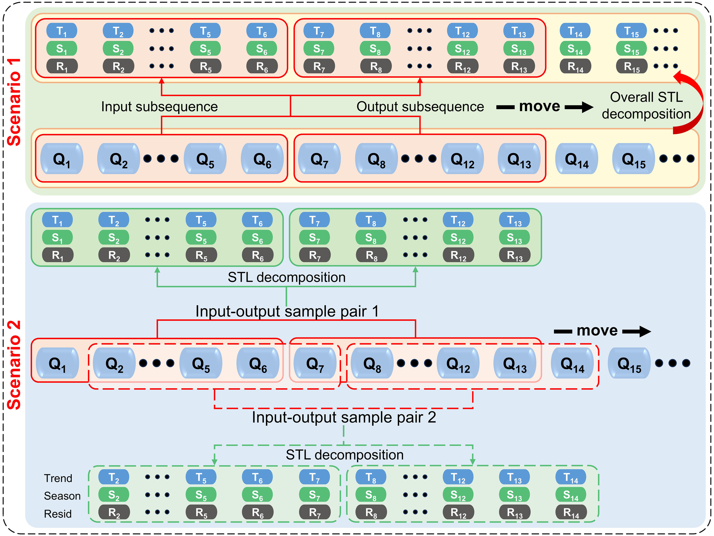
The operation mode of the sliding window and scenario settings. Window size of 6 is used as an example.
2.3 Seasonal and trend decomposition using loess
STL is a widely used and robust method for decomposing time series, in which loess (locally weighted regression) is a method for estimating nonlinear relations. The STL decomposition method was proposed by Cleveland and Cleveland (1990), and has several advantages: STL can handle any type of seasonality, not just monthly and quarterly data; seasonal items can change over times; and the rate of change can be easily controlled. STL was used to decompose the time series of Yellow River inflow into three items: trend term, seasonal term, and residual term (Equation 5).
where the original time series data, seasonal components, trend components and residual components are expressed as , , , and . They range from 1 to N (sequence length). The key of the STL algorithm is locally weighted regression, which combines the simplicity of traditional linear regression and the flexibility of nonlinear regression to fit a smooth two-dimensional scatter map. The process of the decomposition algorithm is shown in Figure 2.
Figure 2
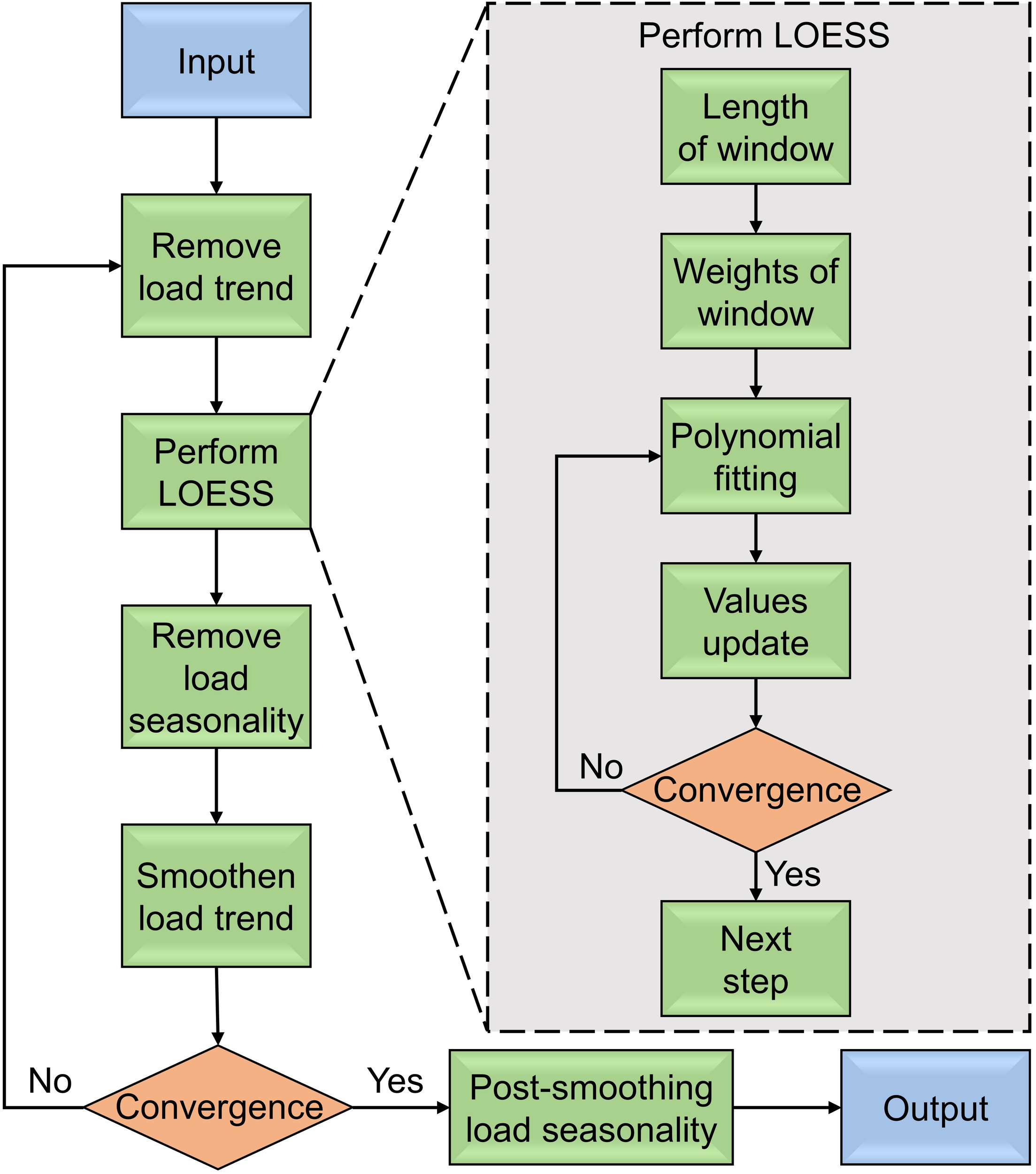
The process of the STL algorithm.
2.4 Light gradient boosting machine
Light gradient boosting machine (LightGBM) was originally developed jointly by Microsoft and Peking University to solve the problems of efficiency and scalability of the gradient boosting decision tree (GBDT) when applied to high-dimensional input characteristics and large amounts of data (Ke et al., 2017). LightGBM does not use information gain to segment the internal nodes of each tree as traditional GBDT does. LightGBM combines two innovative techniques: gradient-based one-side sampling (GOSS) and exclusive feature bundling (EFB) to segment internal nodes. For the GOSS algorithm, a is the proportion of larger gradient samples, and is the proportion of randomly selected smaller gradient samples, and the distribution is divided into data sets A and B. When calculating the information gain, it is necessary to ensure that discarding some samples with smaller gradients will not affect the model training, thus the coefficient will be multiplied by the reserved smaller gradient samples. After the last iteration, the sample data are sorted in descending order of gradient. The final calculated gain is as follows (Equation 6):
where , and denotes the negative gradients of the loss function for the LightGBM outputs in each iteration.
In addition to using GOSS for sampling, LightGBM uses EFB to speed up the training process without losing accuracy. Many applications have high and sparse input features that are mutually exclusive at the same time (i.e., these features cannot be non-zero at the same time). However, the EFB algorithm can bind mutually exclusive features in data sets to form a low-dimensional feature set, which can effectively avoid the calculation of zero-value features. In the algorithm, a table recording non-zero features can be established for each feature. By scanning the data in the table, the time complexity of creating a histogram can be effectively reduced. These two algorithms solve the problem of the number of data and the number of data features, respectively. Compared to other tree-based models such as XGBoost and Random Forest, LightGBM offers faster training speed and superior processing capability for large-scale time series data. Previous studies have demonstrated its strong performance in hydrological forecasting, particularly in inflow prediction, where it effectively captures nonlinear relationships and temporal dependencies (Ke et al., 2017). In the current study, the input and output variables of the LightGBM models were historical flow and future flow, respectively, while the input and output variables of the STL–LightGBM models were historical flow and its terms of STL decomposition and future flow, respectively. A training-testing set division ratio of 6:4 was used, and the data were divided multiple times during model training by the K-Fold (K=5) cross-validation method to alleviate the model’s dependence on specific samples. To improve the model performance, hyperparameter tuning was performed using Python’s Hyperopt library. The Tree-structured Parzen Estimator (TPE) algorithm was used to efficiently search the hyperparameter space for the best combination to enhance the generalization ability and prediction accuracy of the model.
3 Case study
3.1 Study area and data
Here, a case study was conducted for the Lijin hydrological station (Figure 3). Lijin Station (37°31′37.2″ N, 118°18′29.52″ E), located in Dongying, Shandong Province, China, 104 km from the estuary of the Yellow River, is the last hydrological station before the Yellow River enters the Bohai Sea. We collected the inflow as raw experimental dataset records (data source: http://www.yrcc.gov.cn/) obtained every day (from January 2009 to December 2021). The Yellow River has the largest amount of sediment in the world (Qiu et al., 2024), and part of the land in Dongying is formed from deposition from the Yellow River (Wang and Sun, 2021). The Yellow River has historically flooded from time to time. The river outflow also transports many nutrients into the Bohai Sea, affecting the health of the marine ecological environment (Yang F. X. et al., 2024). Hypoxia often occurs in the Bohai Bay, mainly because of the considerable pollution burden (Wang et al., 2023; Wei et al., 2019; Wu et al., 2022). If some flow data can be predicted in advance, decision-makers can be prepared to avoid and reduce some unnecessary losses and disasters. Because the YRE is fed from a wide range of river basins, the temporal and spatial characteristics of the variables affecting the inflow are difficult to identify. This study aims to explore the potential of the STL–LightGBM approach by using only inflow time series data, allowing for a clearer evaluation of the STL algorithm and LightGBM model without interference from external variables. This approach helps isolate the model’s core mechanisms, reduces complexity, enhances generalization. Therefore, to predict the inflow efficiently and succinctly, no additional features (such as precipitation and temperature) were used in this study. The aim of the study was to predict future inflow through historical inflow data and its terms of STL decomposition.
Figure 3
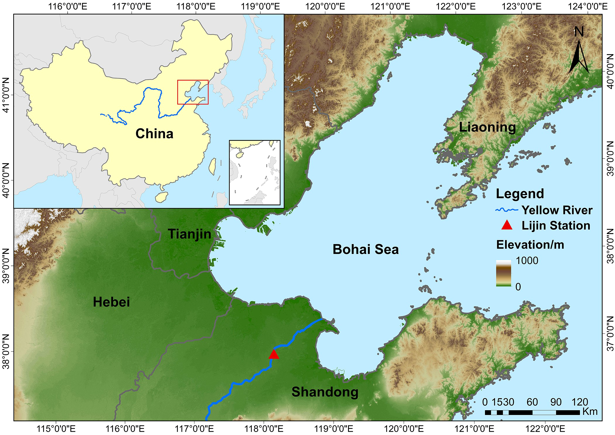
Map of the YRE and the location of Lijin Station.
3.2 Open-source software and performance metrics
This study relied on Python 3.7 open-source libraries, including Numpy, Math, and Pandas. Statsmodels was used to compute the ACF, PACF and STL. The LightGBM and Sklearn packages were used to implement LightGBM and SW. Matplotlib and Seaborn were used to draw figures. The packages were installed using Anaconda on the Windows 10 system. All the experiments were conducted on a workstation equipped with an Intel i5-10600KF CPU, a 16 GB RAM, and an NVIDIA GTX Geforce 3060 (12GB) GPU.
In this study, the Nash-Sutcliffe efficiency (NSE) and root mean square error (RMSE) were used to evaluate the performance of the LightGBM and STL–LightGBM models. These measures were defined by the following formulas (Equations 7, 8):
where represents the observed data, is the value of prediction, and and denote the mean observed and predicted values, respectively.
3.3 Predicting variable selection
The selection of input variables is very important for time series prediction (Tran et al., 2015). In this study, ACF was used to calculate the time lag of inflow. Figure 4 showed the autocorrelation functions and partial autocorrelation functions for various lag numbers at the Lijin Station. There was significant autocorrelation in the flow into the sea at different times. The ACF thresholds of ≥0.7, ≥0.6, and ≥0.5 represent different levels of autocorrelation in time series, commonly used to assess the temporal dependence of data in time series modeling. The PACF further validates the lag windows determined by the ACF, ensuring that the selected lags effectively capture the most significant historical information in the time series. Considering PACF and ACF comprehensively, we used different time delays (input variables) and different lead times (output variables) to train the machine learning model, as detailed in Table 1.
Figure 4
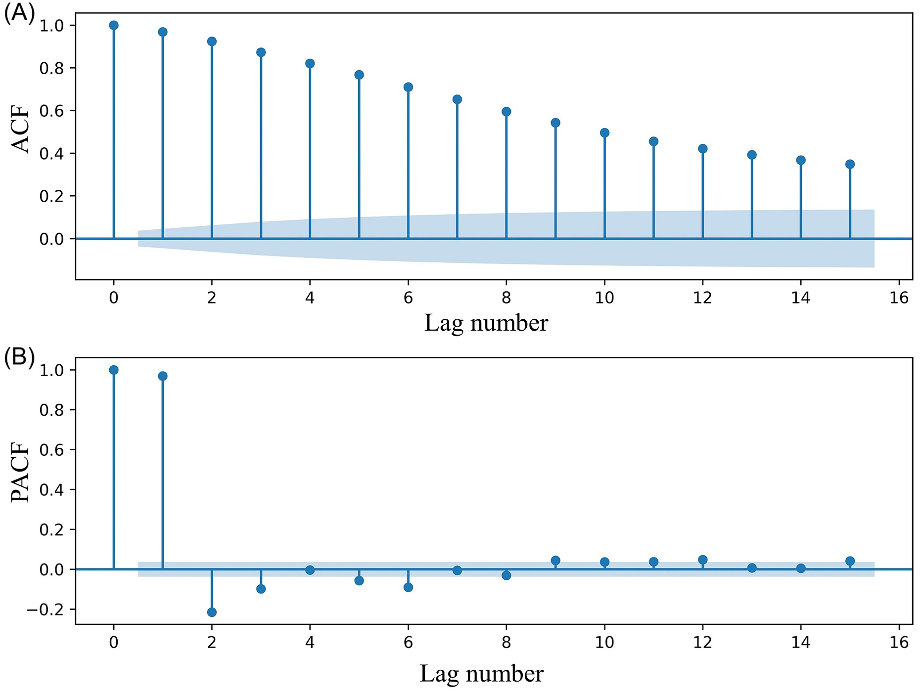
ACF (A) and PACF (B) of the runoff of Lijin Station. The shaded area in the figures indicates the ± 95% confidence level.
Table 1
| Sliding windows (days) | Leading time (days) | ACF | Model |
|---|---|---|---|
| 6 | 1-7 | >=0.7 | LightGBM6 |
| 8 | 1-7 | >=0.6 | LightGBM8 |
| 12 | 1-7 | >=0.5 | LightGBM12 |
Sliding window size based on ACF value.
3.4 STL pre-processing methods
The time-series flow data were divided into a 60% training set and a 40% test set. The effects of different STL application scenarios on the performance of the machine learning model were compared. The following scenarios were set (Figures 1, 5).
Figure 5
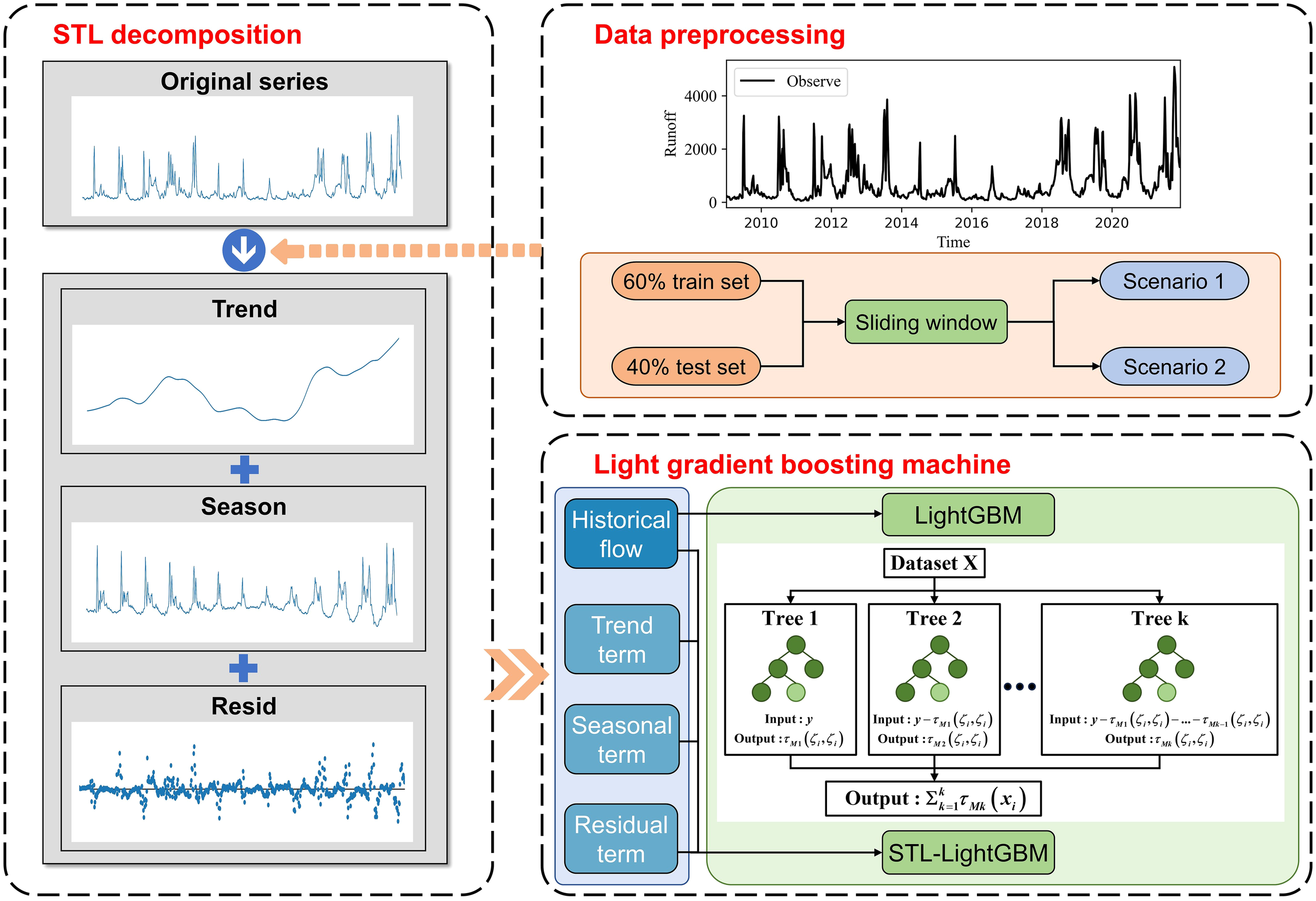
Structure of the technique used in this study.
Scenario 1: The original data set was divided into a training set and test set, and the training set and test set were processed into input and output subsequence through the time SW. The training set and test set were decomposed by STL. The historical flow ( to ) and decomposition terms (trend term, seasonal term, and residual term) were used as input variables of the model, and the future flow () was used as the output variable to train and test the model (abbreviated as S1).
Scenario 2: The original data set was divided into a training set and test set, and the training set and test set were processed into input and output subsequence through the time sliding window. For the training set and test set, each sample pair was decomposed by STL. Its historical flow ( to ) and its decomposition term were taken as input variables of the model, and its future flow () was used as output variable to train and test the model (abbreviated as S2). As shown in Figure 1, during the training process, the model can only use historical data from the training set and does not access any information from the test set. In the testing phase, the trained model is used exclusively for prediction without refitting or adjusting parameters based on the test data, thereby preventing information leakage.
Another scenario decomposed the original data set into new data by STL. The data generated by STL were divided into a training set and a test set. The model was trained and tested by using the time SW as the input and output subsequence. The results of this scheme and scenario 1 were similar and will not be repeated in this study.
4 Results
4.1 Results of time autocorrelation
For a time series, whether the data series has time autocorrelation or not should be determined (Apaydin et al., 2021). Figure 4A shows the autocorrelation diagram of the inflow, wherein the horizontal axis represents the number of delay periods (days), and the longitudinal axis represents the autocorrelation coefficient. This is located on one side of the zero axis for a long time, which is a typical characteristic of a monotone trend series. At the same time, there is an obvious fluctuation pattern, which is typical of strong autocorrelation of a time series with periodic variation. The time series is also a non-stationary series that contained a trend, seasonal, or periodic series. We used the STL decomposition algorithm to extract the time characteristics in preparation for the establishment of the machine learning model.
4.2 STL analysis
In this study, STL was used to improve the prediction potential of the model. Figure 6 shows the decomposition results using the STL method of the data series of the Yellow River flow data. As shown in Figure 6, the seasonal component exhibits a clear and regular annual cycle, with runoff peaks typically occurring between June and September each year. This seasonal pattern is highly consistent with the hydrological cycle of the Yellow River Basin and is closely related to the annual water and sediment regulation measures (Jia and Yi, 2023; Zhang et al., 2021). Notably, the seasonal component remains relatively stable across different years and was hardly affected by extreme events, indicating that the STL method demonstrates high accuracy and robustness in extracting seasonality from time series data. From 2015 to 2017, the trend component shows a significant downward trend. This change in trend corresponds to fluctuations in the residual component, suggesting that the fundamental pattern of runoff in the Yellow River may have undergone changes during this period. The residual component captures abnormal variations beyond the trend and seasonality. During extreme runoff events, the residuals exhibit marked deviations, especially from June to September each year, showing sharp fluctuations.
Figure 6
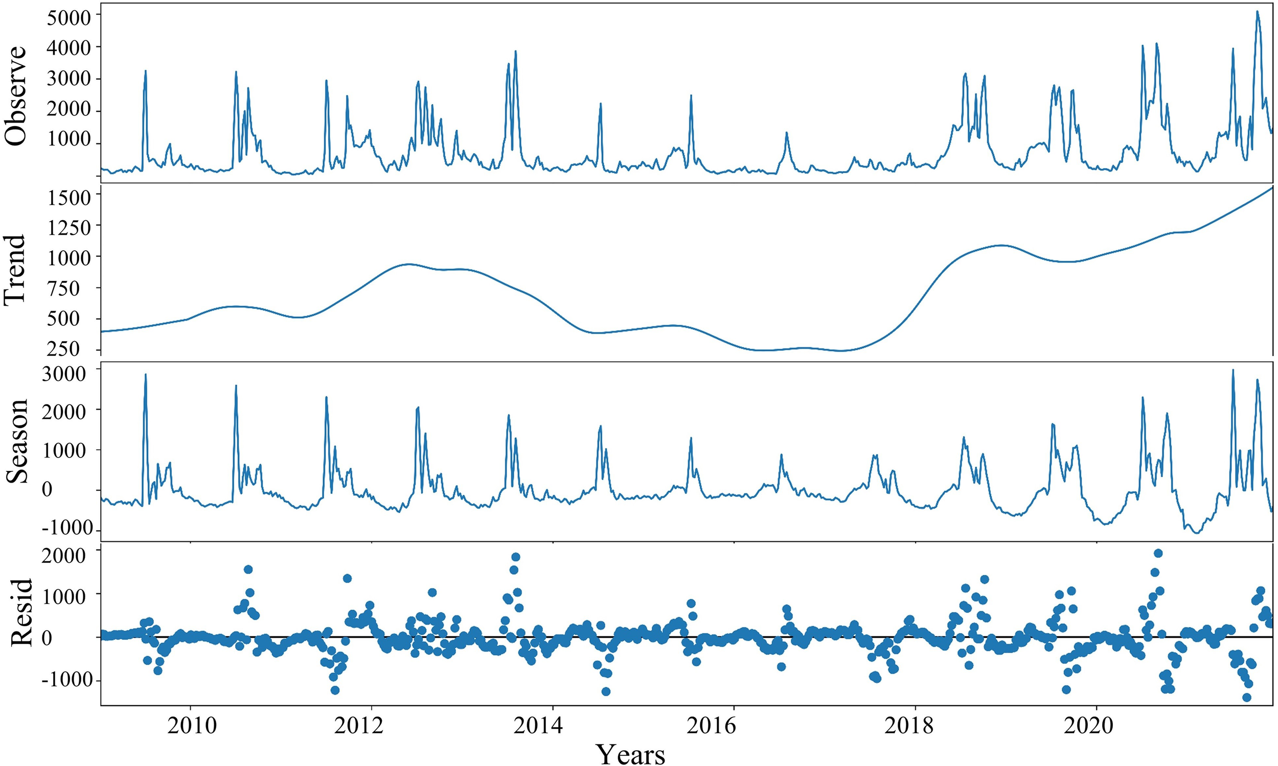
Decomposed daily runoff using the STL method.
4.3 Model cross-validation
Cross-validation algorithm was employed, by dividing the whole dataset to 5-sub classes, to check the accuracy and robustness of the models. The cross-validation process was consistent across different models, and the results were similar. Therefore, the analysis was focused solely on the S2-LightGBM8 model. Figure 7A illustrates the 5-fold cross-validation process of the TPE algorithm for searching the optimal structure of the S2–LightGBM8 model. The lowest RMSE value was recorded in the first fold. Among different lead times, the RMSE values of L1 were the lowest, indicating the best performance in short-term prediction. The RMSE values of L4 were moderate, while L7 exhibited high RMSE values, suggesting that prediction accuracy decreased as the lead time increased. Figure 7B shows the variation of RMSE values with iteration under different lead times. After the Fifteenth iteration, a significantly decrease in RMSE was observed, followed by a stable trend with further iterations. The decline in RMSE values indicated the high efficiency of the TPE algorithm in optimizing parameters and tuning the structure of the S2–LightGBM8 model.
Figure 7
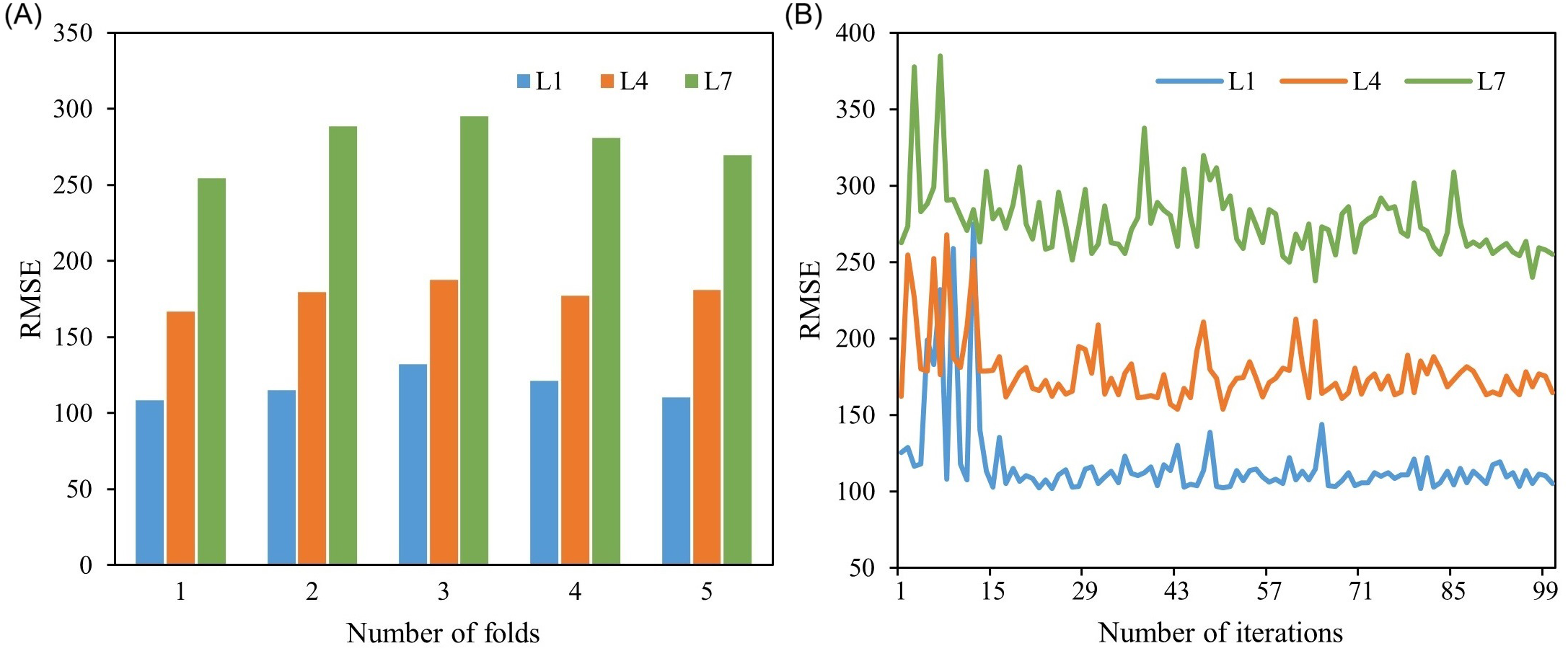
Cross-validation results of the S2-LightGBM8 model: (A) RMSE by number of folds; (B) RMSE variation with iterations. L1, L4, and L7 respectively represent 1-day lead time, 4-day lead time, and 7-day lead time.
4.4 Model performance under different SW
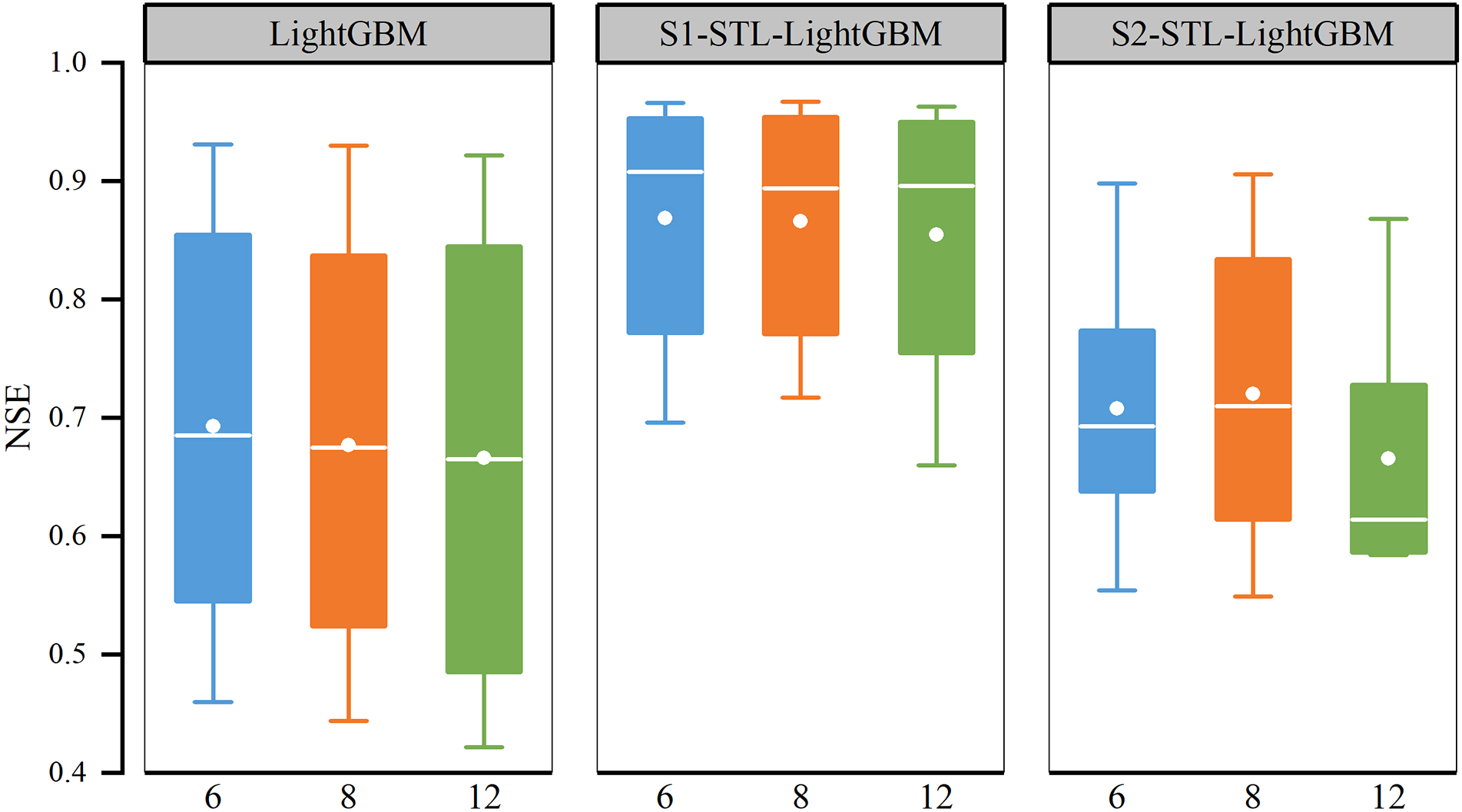
The prediction performance of the original model (LightGBM) and the STL–LightGBM model under different SW (LightGBM6, STL–LightGBM6, LightGBM8, STL–LightGBM8, LightGBM12, STL–LightGBM12) were compared, and the best SW of the model was determined based on the NSE and RMSE. The results showed that the prediction performance of the LightGBM model and STL–LightGBM varied with the size of SW (Tables 2, 3). When the lead time of S1–STL–LightGBM was less than 2 days, the S1–STL–LightGBM8 performed better. For example, when the lead time was 2 days, the NSE (RMSE) of S1–STL–LightGBM8 was 0.954 (211.342), which was better than that of the other SW models. When the lead time was 3–5 days, S1–STL–LightGBM6 had the best performance, with the best values of NSE (0.941, 0.908, and 0.845) and RMSE (239.763, 299.538, and 389.868). The overall performance of the model was reflected by the mean value. S1–STL–LightGBM6 had the highest average NSE (0.869) and the lowest average RMSE (334.883). S2–STL–LightGBM was similar to S1–STL–LightGBM. When the SW was 8 days, the performance was slightly better when predicting short-term flow (lead time: 1–4 days), but the performance decreased with the increase in the lead time. It is observed that the overall effect of STL–LightGBM8 was better than the other SW models in S2 (Figure 8), and the model was more robust. In addition, according to the results of the autocorrelation analysis (Figure 4), when the prediction factor (input) was closer to the target variable (output), the contribution of the model was greater, and there was a higher autocorrelation. This result was similar to that of Chen et al. (2020). The results also showed that the flow of the Yellow River into the sea could be predicted by time autoregressive machine learning based on a single variable.
Table 2
| Metric | Model | Lead time (days) | ||||||
|---|---|---|---|---|---|---|---|---|
| 1 | 2 | 3 | 4 | 5 | 6 | 7 | ||
| NSE | LightGBM6 | 0.931 | 0.855 | 0.766 | 0.685 | 0.608 | 0.545 | 0.460 |
| STL-LightGBM6 | 0.966 | 0.953 | 0.941 | 0.908 | 0.845 | 0.772 | 0.696 | |
| LightGBM8 | 0.930 | 0.837 | 0.743 | 0.675 | 0.585 | 0.524 | 0.444 | |
| STL-LightGBM8 | 0.967 | 0.954 | 0.924 | 0.894 | 0.837 | 0.771 | 0.717 | |
| LightGBM12 | 0.922 | 0.845 | 0.718 | 0.665 | 0.606 | 0.485 | 0.422 | |
| STL-LightGBM12 | 0.963 | 0.950 | 0.929 | 0.896 | 0.830 | 0.755 | 0.660 | |
| RMSE | LightGBM6 | 260.377 | 376.581 | 478.825 | 555.302 | 619.537 | 667.800 | 727.755 |
| STL-LightGBM6 | 181.516 | 214.669 | 239.763 | 299.538 | 389.868 | 472.955 | 545.873 | |
| LightGBM8 | 261.633 | 399.182 | 502.262 | 564.332 | 637.923 | 683.061 | 738.251 | |
| STL-LightGBM8 | 179.635 | 211.342 | 273.444 | 322.232 | 399.969 | 473.608 | 526.772 | |
| LightGBM12 | 276.437 | 389.842 | 525.924 | 572.863 | 621.572 | 710.940 | 752.975 | |
| STL-LightGBM12 | 190.956 | 221.322 | 264.687 | 318.871 | 408.116 | 490.345 | 577.543 | |
Performance statistics using LightGBM and S1-STL–LightGBM for predicting flow at 1 to 7 days ahead during the testing period.
Table 3
| Metric | Model | Lead time (days) | ||||||
|---|---|---|---|---|---|---|---|---|
| 1 | 2 | 3 | 4 | 5 | 6 | 7 | ||
| NSE | LightGBM6 | 0.931 | 0.855 | 0.766 | 0.685 | 0.608 | 0.545 | 0.460 |
| STL-LightGBM6 | 0.898 | 0.774 | 0.724 | 0.693 | 0.675 | 0.638 | 0.554 | |
| LightGBM8 | 0.930 | 0.837 | 0.743 | 0.675 | 0.585 | 0.524 | 0.444 | |
| STL-LightGBM8 | 0.906 | 0.834 | 0.776 | 0.710 | 0.653 | 0.614 | 0.549 | |
| LightGBM12 | 0.922 | 0.845 | 0.718 | 0.665 | 0.606 | 0.485 | 0.422 | |
| STL-LightGBM12 | 0.868 | 0.728 | 0.676 | 0.584 | 0.614 | 0.603 | 0.586 | |
| RMSE | LightGBM6 | 260.377 | 376.581 | 478.825 | 555.302 | 619.537 | 667.800 | 727.755 |
| STL-LightGBM6 | 316.467 | 470.386 | 519.787 | 548.182 | 564.132 | 596.041 | 661.442 | |
| LightGBM8 | 261.633 | 399.182 | 502.262 | 564.332 | 637.923 | 683.061 | 738.251 | |
| STL-LightGBM8 | 304.129 | 403.531 | 469.065 | 533.411 | 583.064 | 615.244 | 664.881 | |
| LightGBM12 | 276.437 | 389.842 | 525.924 | 572.863 | 621.572 | 710.940 | 752.975 | |
| STL-LightGBM12 | 360.064 | 516.345 | 564.006 | 638.719 | 615.624 | 624.365 | 637.180 | |
Performance statistics using LightGBM and S2-STL–LightGBM for predicting flow at 1 to 7 days ahead during the testing period.
Figure 8
Performance of the projected LightGBM and STL–LightGBM models. X-axis (6, 8, and 12) represents the size of the sliding window.
4.5 Comparison of prediction results at different lead times
To compare the effects of different lead times on the prediction performance of models, Figure 9 shows the prediction results of the model with a window size of 8 and the lead time of 1, 4, and 7 days, respectively. When the lead time was 1 day (Figure 9A), the predicted values of the three models fitted well with the observed values, and the overall fitting effect was satisfactory. The results showed that the three models were able to use the historical flow for 8 days as an input variable to predict the flow into the sea in the next 1-day period. Figure 9B shows the fit of the predicted value of the model with the real value with a lead time of 4 days. The prediction results were worse than those with a forecast period of 1 day, and the original model (LightGBM) was also the worst of all the models. The prediction with low inflow was better than that with high inflow. Compared with other forecast periods, the prediction effect of the 7-day lead time was the worst, especially the prediction near the peak, where most of the sample forecasts underestimated the observed value (Figure 9C). The results showed that the performance of all the models decreased in varying degrees with an increase in the lead time. In other words, the accuracy of models in predicting the inflow of the Yellow River into the sea in the coming 7 days was lower than that for the next 1-day period.
Figure 9
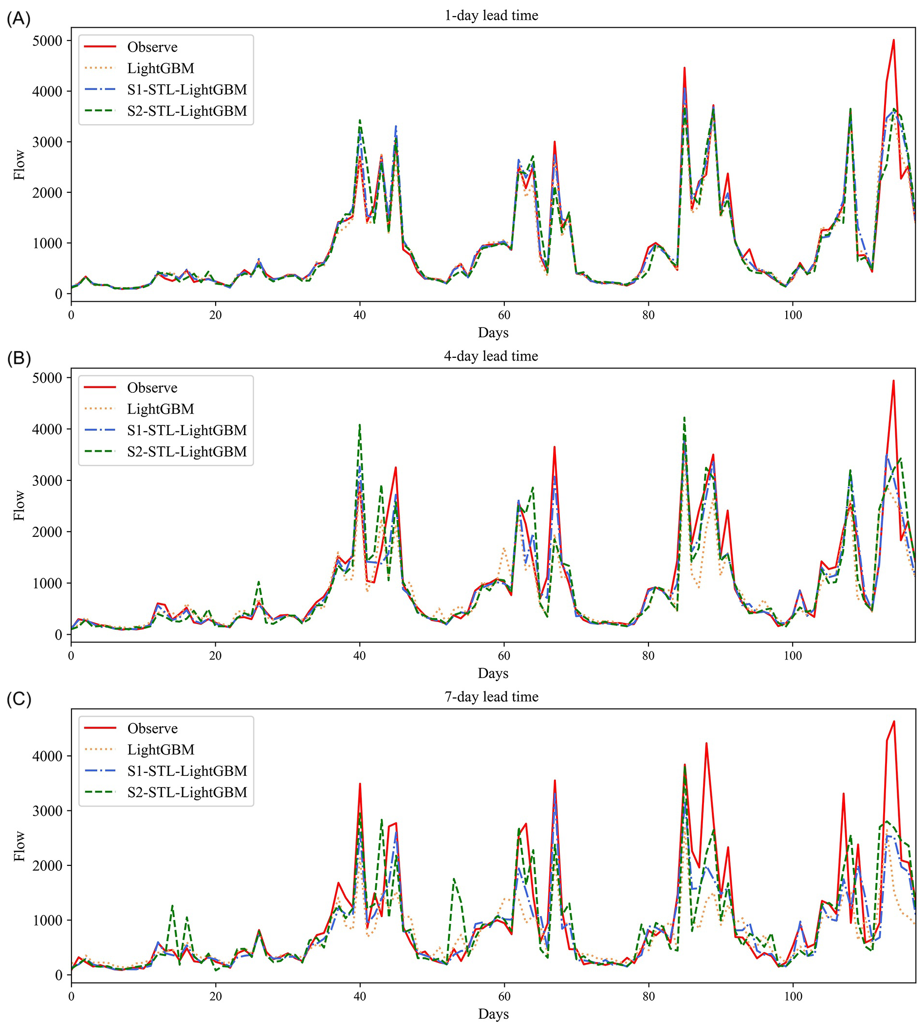
Predicted and observed runoff time series with prediction lead times ranging from 1 to 7 days using LightGBM and STL–LightGBM during the testing period: (A) 1-day lead time; (B) 4-day lead time; and (C) 7-day lead time.
Taylor diagrams of three models were drawn to measure the changes in model performance with different lead times (Figure 10). Taylor diagrams are often used to evaluate the accuracy of models, and the commonly used accuracy indicators are the correlation coefficient, standard deviation, and RMSE. As shown in Figure 10A, the distance on the diagram of the three models was relatively close, the results were good, and the correlation coefficients all reached more than 0.95. For the predicted value, the standard deviation was close to 1, indicating that the performance was relatively stable. Figure 10A shows that all three models could well predict the inflow into the sea in the next 1-day period. However, with the extension of the lead time, the scatter points of the three models become dispersed, indicating a decline in their predictive performance (Figures 10B, C). Especially when the lead time was 7 days, the correlation coefficient of the original model (LightGBM) was less than 0.75, indicating that the original model could not predict the sea flow on the seventh day.
Figure 10
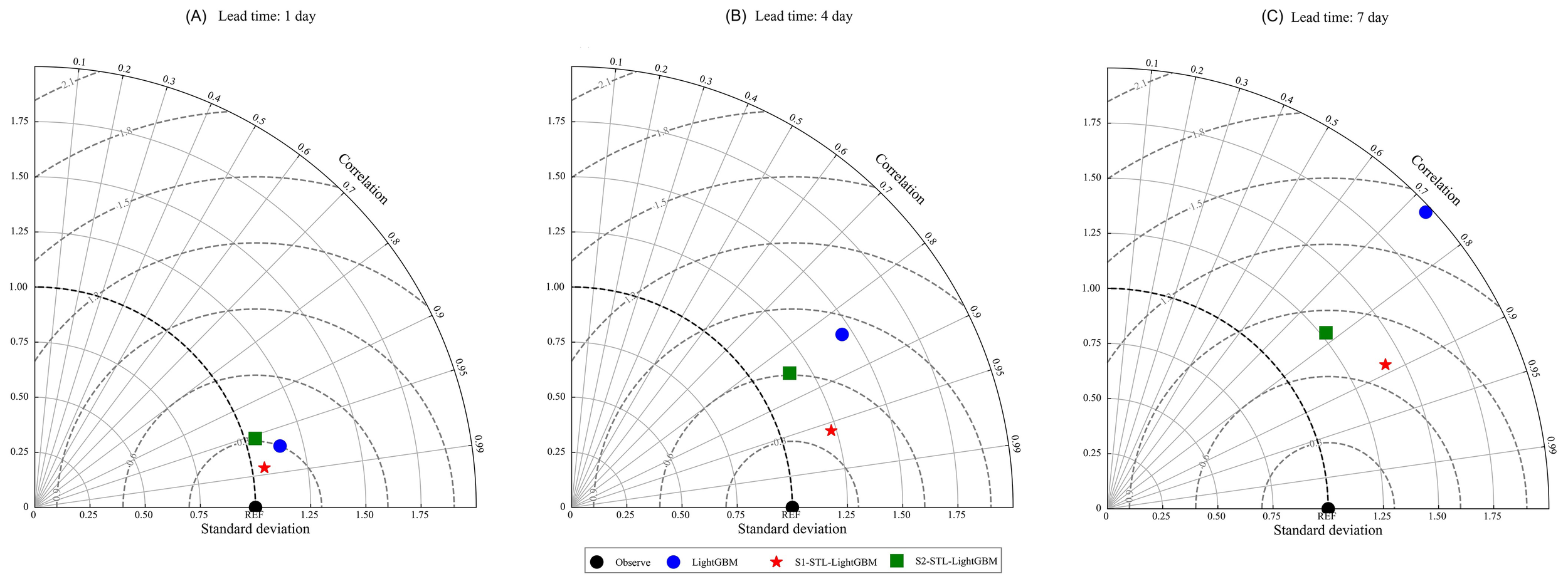
Taylor diagram of the model performance: (A) 1-day lead time; (B) 4-day lead time; and (C) 7-day lead time. The scatter in the Taylor diagram represents the model, the radiation represents the correlation coefficient, the horizontal and vertical axes represent the standard deviation, and the dotted line represents the root mean square error.
4.6 Comparison of prediction performance between STL–LightGBM and LightGBM
From the above analysis and discussion, STL technology was observed to have significantly improved the prediction ability of the LightGBM model. In this section, we discuss the improvement of the original model in different scenarios and the reasons for it. We found that the performance of the model decreased with the growth of the lead time, but the decline in the S1–STL–LightGBM performance was less than that of the original model. From the radar diagram (Figure 11), we can observe that with the extension of the lead time, the improvement of the LightGBM model by S1–STL increased gradually. At the lead time reached seven days, the NSE of S1–STL was approximately 0.3 higher than that of the LightGBM model. In addition, we can observe that when the lead time was 4 days and 7 days, the S1–STL–LightGBM was much better than the original model (Figures 8, 9). This also confirms that the S1–STL scheme can effectively improve the long-term prediction ability of the original model.
Figure 11
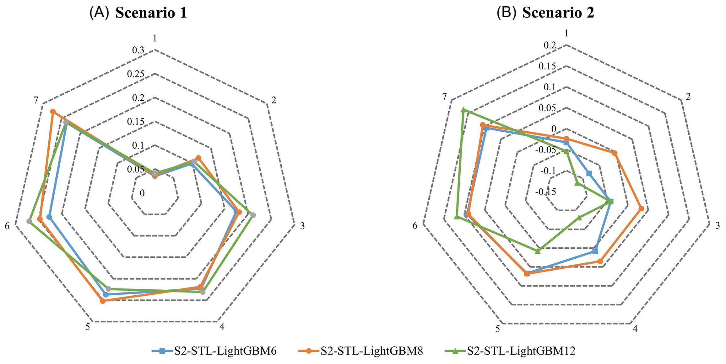
Radar diagram of the model performance for Scenarios 1 (A) and Scenarios 2 (B). The dotted line represents the NSE difference between the STL–LightGBM model and the LightGBM model.
The promotion ability of S2–STL was, however, different from that of S1–STL. Through Figure 11, we can clearly observe that S2–STL did not improve the prediction ability of the original model 3 days before the lead time and it reduced the accuracy. When the lead time reached the fourth day, the prediction ability of S2–STL was greater than that of the original model. For example, when the forecast period was 7 days, the S2–STL–LightGBM8 increased by 0.105 compared with the NSE of the LightGBM8 model (Table 3), and the result was satisfactory. From the above results, we can also conclude that both S1–STL and S2–STL improved the long-term prediction ability of the original model. In other words, STL can help address the problem that the performance of the model decreases as the lead time increases.
5 Discussion
5.1 Effect of different lead times on model performance
In general, the prediction performance of inflow models decreases as the lead time increases, which is also the case in our study. Figures 8, 9 clearly show that all models could predict flow for 1-day lead time. However, with the increase of the lead time, the prediction ability of models declined. This was because when the lead time was short, there was a simple linear relationship between t day and : flow into the sea, and thus all the models could predict the 1-day flow ( day). Therefore, there was no significant difference in the prediction effect of different models with a 1-day lead time.
However, with the extension of the lead time, the autocorrelation of time flow series weakened rapidly, the correlation between : and became complex and nonlinear, and the performance of the model decreased. The inflow of the Yellow River into the sea is affected by the climate of the mainstream of the Yellow River every year, and the annual rainfall is different as is the inflow into the sea (Wang et al., 2024; Wang and Sun, 2021). The flow of the Yellow River into the sea is also influenced by human activities (Shi et al., 2019), such as reservoir regulation, urbanization, agricultural practice, soil and water conservation measures, and mining (Dou et al., 2023; Wang and Cheng, 2022; Wu X, et al., 2023; Xin and Liu, 2022; Yu et al., 2021). We assumed that obtaining more data through various techniques, such as upstream reservoir operation, precipitation, may improve the predictive performance of the model.
5.2 Data leakage in time series preprocessing
STL decomposition, as a classical time series preprocessing method, relies on global trend fitting and seasonal smoothing. Studies have pointed out that any smoothing operation applied to the entire test set may introduce data leakage during the testing phase (Yang X. Y. et al., 2024). Therefore, if STL decomposition is performed on the entire test set at once during testing, the decomposition result of a given sample may be influenced by future observations. This essentially introduces future information into the model, which is equivalent to the model “seeing the future” during training or testing. Such a practice violates the fundamental assumption of causality in time series forecasting, which requires models to be trained solely on historical data, and may thus result in misleading evaluations of model performance (Qian et al., 2019). However, many existing studies have not fully recognized the potential data leakage issues arising from using decomposition methods such as STL on the entire test set, which may lead to overestimation of the improvements these methods bring to machine learning models (Apaydin et al., 2021; Chen Z, et al., 2021; Zuo et al., 2020).
To address this issue, we proposed a stepwise decomposition strategy (S2–STL), which ensured that, at each time point, STL decomposition only utilized the current and past observations to extract trend and seasonal components. This guaranteed that the generated features did not contain any future information and strictly adhered to the causality constraints required for time series modeling (see Figure 1). Theoretically, S2–STL could be regarded as a recursive adaptation of STL’s local smoothing philosophy, where the sliding window moved forward with time, relying solely on historical observations to simulate the real information boundaries in forecasting tasks. Compared with global decomposition approaches, stepwise decomposition offered distinct advantages in model generalization and stability. This strategy has already been validated in meteorological time series (Wang and Wu, 2016) and hydrological runoff forecasting (Quilty and Adamowski, 2018).
Results demonstrated significant differences in model performance between S1–STL and S2–STL. In S1–STL, STL was first applied to the entire test set before generating input-output pairs through a sliding window, which meant that each input variable’s trend, seasonal, and residual components may implicitly contain future information from the target variable. This process provided the model with prior signals that were unavailable in actual forecasting scenarios, resulting in systematically underestimated test errors and overestimated generalization capabilities. Similarly, seasonality patterns extracted from the full dataset reduce the learning burden for the model, thereby exaggerating the performance gains attributed to STL decomposition. In contrast, S2–STL performed recursive decomposition based solely on historical data, effectively preventing future information leakage and providing an accurate representation of the decomposition strategy’s true utility in real-world forecasting tasks.
In conclusion, S2–STL not only adhered strictly to the causality principle inherent in time series forecasting but also effectively mitigated the risks of information leakage due to improper preprocessing, making it a rigorous and reliable strategy for time series decomposition.
5.3 The role of STL in predicting inflow into the sea
This study used the STL method for time series decomposition. Although methods like empirical mode decomposition (EMD), SSA, and wavelet transform (WT) are also widely applied, they differ significantly from STL in terms of decomposition logic and applicability. EMD often produces unstable decomposition results when handling time series with strong trends and is not suitable for extracting long-term trends (Yang X. Y. et al., 2024). SSA is computationally intensive, primarily used for signal denoising rather than specifically designed for seasonal decomposition, and requires complex hyperparameter adjustments. While WT is suitable for non-stationary data, the choice of wavelet basis significantly impacts the decomposition results (Quilty and Adamowski, 2018), adding complexity to its application. In contrast, STL provides a clear mathematical formulation, does not rely on parameter selection, is applicable to data of different time scales, and can reliably decompose trend and seasonal components. Regarding data leakage, this study specifically investigated the potential data leakage when time series decomposition methods were combined with machine learning models. Our research found that unreasonable decomposition strategies may lead to data leakage. S2–STL avoided data leakage through stepwise decomposition, offering a rigorous and practically applicable decomposition strategy for forecasting tasks. While other decomposition methods follow different mechanisms that may lead to different data leakage patterns and require further research.
Through the pre-processing of the time series (Apaydin et al., 2021), we observed that the inflow data of the Yellow River into the sea was a non-stationary time series, which contained trend, seasonality, or periodicity. STL decomposed the original dataset into trend items, seasonal terms, and residual terms based on loess. These data combined with historical observation data made the characteristics of the input samples more abundant. STL was very resilient to outliers in the inflow data, resulting in a robust component subseries. The robustness of components could be translated into enhanced prediction accuracy for these subseries of prediction methods. The newly generated series reflected the seasonality and trend characteristics of the original data, and then improved the prediction ability of the model (He et al., 2021).
Inflow exhibits distinct periodic variations, and extracting the seasonal component helps the model better capture cyclic patterns, reducing prediction errors caused by periodic changes in the data. The trend component reflects the long-term variations in inflow, providing LightGBM with smooth and stable input features. In long-term forecasting tasks with extended lead times, the original time series may exhibit significant fluctuations. Extracting the trend component helps mitigate short-term disturbances, enhancing the model’s robustness in long-term predictions. This explains why both S1–STL and S2–STL outperform the original LightGBM model in long-term forecasting. The residual component contains non-periodic, random fluctuations. If not properly handled, these residuals may introduce noise and affect the model’s generalization ability. However, STL decomposition effectively separates trend and seasonal signals, allowing LightGBM to focus on learning more representative residual information. This reduces the impact of random fluctuations on the model and enhances its accuracy in long-term predictions.
The difference in the STL decomposition term between S1 and S2 was analyzed from the point of view of the test set value. As shown in Figure 12, we observed that when the input variable of the original test set (test set of LightGBM) was close to the target variable, the correlation was strong, which was consistent with the previous ACF results (Figure 4). The correlation between the seasonal items of S1–STL and the target variable (output) in each lag time was greater than that of historical observation data. It is obviously unreasonable that the characteristics of the data in the sample are leaked owing to the overall STL decomposition of the test set. However, we observed that the correlation between the three STL decomposition items of S2–STL and the target variable increased with the increase of leading time, and the correlation between the seasonal term and the target variable was less than the historical observation data, which may be due to the trend of STL degradation of the sample by loess. Although the improvement of S2–STL was not as strong as that of S1–STL, S2–STL was more in line with the practical application of the model. To sum up, the forecasting ability of STL–LightGBM was better than that of LightGBM, especially the forecast ability (NSE) over 7 days was improved by 0.1. Because STL can improve the problem that the performance of the model decreases with the increase of the lead time, STL can improve the machine learning ability of prediction of the Yellow River’s inflow into the sea.
Figure 12
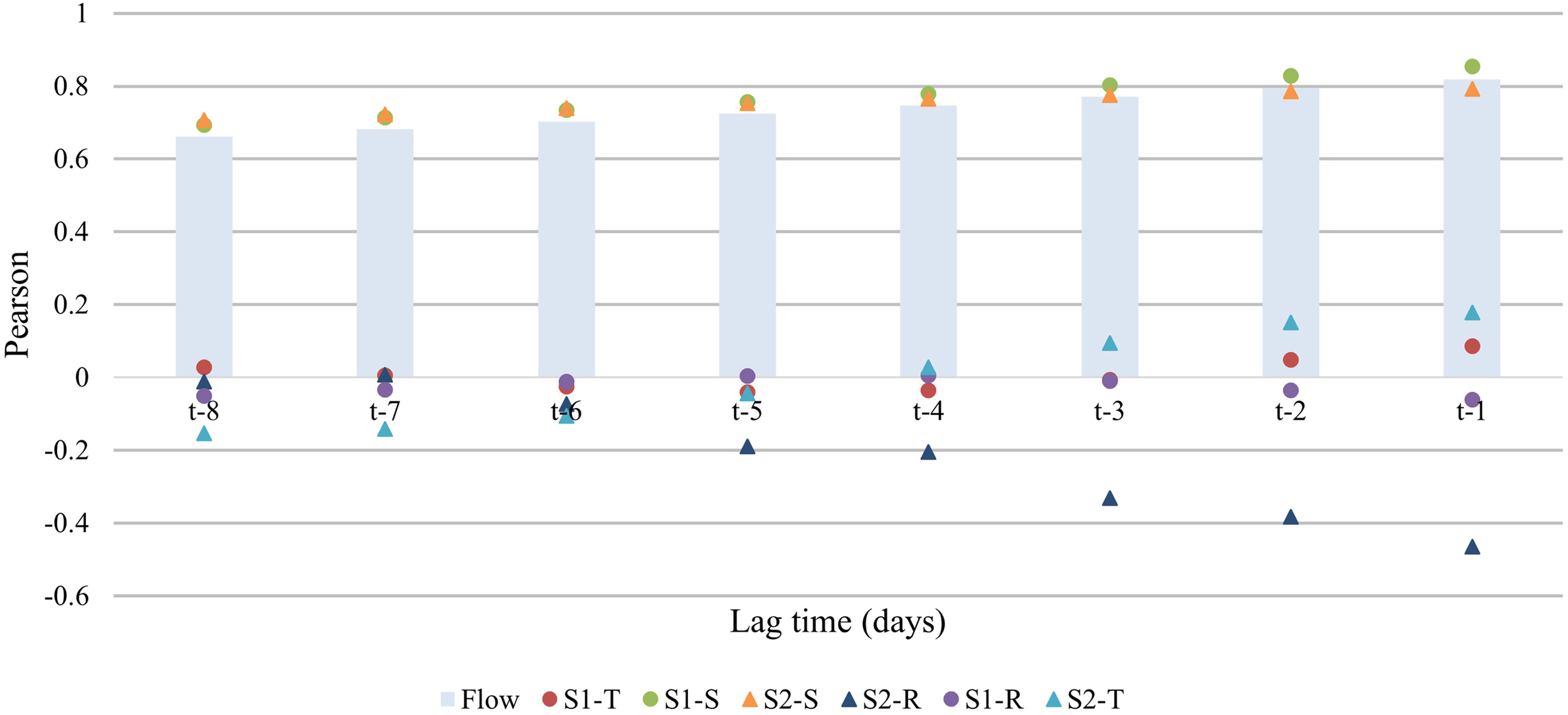
Correlation diagram between decomposition term of STL and the target variable.
5.4 Advantages of STL–LightGBM in predicting coastal inflow
The inflow of the Yellow River plays a crucial role in shaping the offshore ecosystem’s health of the Bohai Sea. As shown in Figure 6, due to the short-term interruption of Water-Sediment Regulation Scheme (WSRS) from 2015 to 2017, the discharge into the sea showed a declining trend during this period (Wang J. J. et al., 2022). This further highlights the significant regulatory role of WSRS in the hydrological processes of the LYR. These changes also had a notable impact on the seasonal pattern of the Yellow River, altering its natural flow regime and affecting the timing and magnitude of inflow variations. During the WSRS, the Yellow River transported over 20% of the annual discharge and 60% of the annual sediment load to the YRE (Liu et al., 2012; Li and Sheng, 2011). This sudden large input has significantly altered the physical and chemical characteristics of the estuary, affecting the ecological balance of the Bohai Sea (Yang F. X. et al., 2024). These ecological changes not only have a profound impact on the Bohai Sea’s ecosystem but also directly affect the sustainable development of fisheries and regional environmental health.
Predicting river inflow into the sea is a key aspect of offshore environmental management (Vinayachandran et al., 2015). The volume of water and sediment discharged during WSRS greatly exceeds that of natural flood seasons (Ji et al., 2020), significantly affecting the spatiotemporal distribution of suspended sediment concentrations (Liu, 2015). The Bohai Sea faces several major ecological issues, such as eutrophication, hypoxia, and sediment pollution, all of which are closely related to river inflows. Additionally, river inflows can impact fish habitats and breeding conditions, and accurately predicting inflow variations can help adjust fishery harvesting plans to prevent overfishing. The STL–LightGBM framework proposed in this study combines STL with the LightGBM model to extract key seasonal and trend patterns from time series data, significantly improving prediction accuracy.
The model proposed in this study used streamflow time series and its decomposition components as input variables, without relying on external factors such as regional meteorology, topography, soil, or human activities. This enhances the model’s transferability across different regions. The results showed that the inflow data itself exhibits significant temporal autocorrelation (Figure 4), meaning that future streamflow can be effectively predicted based solely on past streamflow data. For example, in short-term flow forecasting for the Yellow River Basin, accurate predictions can be made using only the past 7–14 days of streamflow data (Wang et al., 2025). Moreover, previous studies have also confirmed the feasibility of forecasting future runoff based solely on historical streamflow data (Parsaie et al., 2024; Shi et al., 2025; Xu et al., 2024). Therefore, as long as other regions or rivers have sufficient historical streamflow data, the method holds potential for other basins, but further validation is required.
This framework enables early prediction of ecological changes and provides scientific guidance for addressing issues such as hypoxia and eutrophication. Additionally, this prediction technology holds significant potential for offshore environmental monitoring and early warning systems, supporting the management of fisheries resources, water quality maintenance, and ecological protection. It provides a solid foundation for ensuring the long-term health and stability of the Bohai Sea’s ecological environment.
6 Conclusion
In this study, on the basis of the historical single variable of the sea inflow of the Yellow River, STL was used to improve the prediction effect of the machine learning model on future inflow. The main results were as follows:
-
The LightGBM model could predict the recent flow based on the historical inflow of the Yellow River into the sea, and the prediction performance of LightGBM model decreased rapidly with the increase of the lead time. Taking LightGBM8 as an example, the NSEs of 1-, 4-, and 7-day (lead time) were 0.930, 0.675 and 0.444, respectively.
-
STL can improve the prediction ability of traditional machine learning models. In Scenario 2, when the lead time was 6 days and 7 days, the NSEs of STL–LightGBM8 were 0.614 and 0.549, respectively, which are better than that of LightGBM. It is recommended that the STL preprocesses each sample of the test set because this is practical. STL pretreatment of the entire test set overestimated the true performance of the STL–LightGBM.
This study conducted hydrological time series prediction based on data from the Lijin Hydrological Station and obtained several important conclusions. However, some limitations and areas for improvement remain: (1) Choice of decomposition methods: STL was used for time series decomposition, but it is not the only option. Future studies could explore alternatives such as EMD, SSA, or WT to assess their effectiveness in hydrological prediction. (2) Method generalizability: Although the method performed well on data from the Lijin Station, it should be tested on other stations to evaluate its adaptability under different hydrological conditions. (3) Optimization strategies: More advanced techniques, such as Bayesian optimization, could be used to fine-tune key parameters like window size and improve overall model performance. (4) Model extension: Future work could also explore deep learning models like LSTM and Transformer to further enhance predictive capability.
Statements
Data availability statement
Publicly available datasets were analyzed in this study. This data can be found here: http://www.yrcc.gov.cn/.
Author contributions
SW: Conceptualization, Data curation, Methodology, Software, Validation, Visualization, Writing – original draft, Writing – review & editing. KY: Data curation, Methodology, Validation, Visualization, Writing – original draft, Writing – review & editing. HP: Conceptualization, Data curation, Formal Analysis, Funding acquisition, Investigation, Methodology, Resources, Writing – original draft, Writing – review & editing.
Funding
The author(s) declare that financial support was received for the research and/or publication of this article. This study was financially supported by programs of the National Natural Science Foundation of China (grant number U190621) and the Open Research Fund of State Key Laboratory of Simulation and Regulation of Water Cycle in River Basin, China Institute of Water Resources and Hydropower Research (grant number SKL2024YJZD02).
Conflict of interest
The authors declare that the research was conducted in the absence of any commercial or financial relationships that could be construed as a potential conflict of interest.
Generative AI statement
The author(s) declare that no Generative AI was used in the creation of this manuscript.
Publisher’s note
All claims expressed in this article are solely those of the authors and do not necessarily represent those of their affiliated organizations, or those of the publisher, the editors and the reviewers. Any product that may be evaluated in this article, or claim that may be made by its manufacturer, is not guaranteed or endorsed by the publisher.
References
1
Abbasi M. Farokhnia A. Bahreinimotlagh M. Roozbahani R. (2021). A hybrid of Random Forest and Deep Auto-Encoder with support vector regression methods for accuracy improvement and uncertainty reduction of long-term streamflow prediction. J. Hydrol.597, 125717. doi: 10.1016/j.jhydrol.2020.125717
2
Althoff D. Destouni G. (2023). Global patterns in water flux partitioning: Irrigated and rainfed agriculture drives asymmetrical flux to vegetation over runoff. One Earth6, 1246–1257. doi: 10.1016/j.oneear.2023.08.002
3
Apaydin H. Taghi Sattari M. Falsafian K. Prasad R. (2021). Artificial intelligence modelling integrated with Singular Spectral analysis and Seasonal-Trend decomposition using Loess approaches for streamflow predictions. J. Hydrol.600, 126506. doi: 10.1016/j.jhydrol.2021.126506
4
Bai J. H. Xiao R. Zhang K. J. Gao H. F. (2012). Arsenic and heavy metal pollution in wetland soils from tidal freshwater and salt marshes before and after the flow-sediment regulation regime in the Yellow River Delta, China. J. Hydrol.450-451, 244–253. doi: 10.1016/j.jhydrol.2012.05.006
5
Chen X. Huang J. X. Han Z. Gao H. K. Liu M. Li Z. Q. et al . (2020). The importance of short lag-time in the runoff forecasting model based on long short-term memory. J. Hydrol.589, 125359. doi: 10.1016/j.jhydrol.2020.125359
6
Chen S. Ren M. M. Sun W. (2021). Combining two-stage decomposition based machine learning methods for annual runoff forecasting. J. Hydrol.603, 126945. doi: 10.1016/j.jhydrol.2021.126945
7
Chen Z. Xu H. Jiang P. Yu S. N. Lin G. Bychkov I. et al . (2021). A transfer Learning-Based LSTM strategy for imputing Large-Scale consecutive missing data and its application in a water quality prediction system. J. Hydrol.602, 126573. doi: 10.1016/j.jhydrol.2021.126573
8
Cheng X. Y. Zhu J. R. Chen S. L. (2023). Dynamic response of water flow and sediment transport off the Yellow River mouth to tides and waves in winter. Front. Mar. Sci.10. doi: 10.3389/fmars.2023.1181347
9
Cleveland R. B. Cleveland W. S. (1990). STL: a seasonal-trend decomposition procedure based on Loess. J. Off. Stat.6, 3–73.
10
Dou X. Y. Guo H. D. Zhang L. Liang D. Zhu Q. Liu X. T. et al . (2023). Dynamic landscapes and the influence of human activities in the Yellow River Delta wetland region. Sci. Total Environ.899, 166239. doi: 10.1016/j.scitotenv.2023.166239
11
Du K. C. Zhao Y. Lei J. Q. (2017). The incorrect usage of singular spectral analysis and discrete wavelet transform in hybrid models to predict hydrological time series. J. Hydrol.552, 44–51. doi: 10.1016/j.jhydrol.2017.06.019
12
He H. T. Gao S. C. Jin T. Sato S. Zhang X. Y. (2021). A seasonal-trend decomposition-based dendritic neuron model for financial time series prediction. Appl. Soft Comput.108, 107488. doi: 10.1016/j.asoc.2021.107488
13
He F. F. Wan Q. J. Wang Y. Q. Wu J. Zhang X. Q. Feng Y. (2024). Daily runoff prediction with a seasonal decomposition-based deep GRU method. Water16, 618. doi: 10.3390/w16040618
14
Huang L. T. Wang H. X. Liu H. F. Zhang S. A. Guo W. X. (2024). Quantitatively linking ecosystem service functions with soil moisture and ecohydrology regimes in watershed. Sci. Total Environ.955, 176866. doi: 10.1016/j.scitotenv.2024.176866
15
Hyndman R. J. Athanasopoulos G. (2018). Forecasting: Principles and Practice. 2nd Edn (Melbourne, VIC: OTexts). Available at: https://otexts.com/fpp2/ (Accessed March 18, 2024).
16
Jehanzaib M. Ali S. Kim M. J. Kim T. (2023). Modeling hydrological non-stationarity to analyze environmental impacts on drought propagation. Atmos. Res.286, 106699. doi: 10.1016/j.atmosres.2023.106699
17
Ji H. Pan S. Chen S. (2020). Impact of river discharge on hydrodynamics and sedimentary processes at yellow river delta. Mar. Geology425, 106210. doi: 10.1016/j.margeo.2020.106210
18
Jia W. F. Yi Y. J. (2023). Numerical study of the water-sediment regulation scheme (WSRS) impact on suspended sediment transport in the Yellow River Estuary. Front. Mar. Sci.10. doi: 10.3389/fmars.2023.1135118
19
Jiang Z. F. Lu B. H. Zhou Z. G. Zhao Y. R. (2024). Comparison of process-driven SWAT model and data-driven machine learning techniques in simulating streamflow: a case study in the Fenhe River Basin. Sustainability16, 6074. doi: 10.3390/su16146074
20
Jiang S. J. Zheng Y. Solomatine D. (2020). Improving AI system awareness of geoscience knowledge: symbiotic integration of physical approaches and deep learning. Geophys. Res. Lett.47, e2020GL088229. doi: 10.1029/2020GL088229
21
Ke G. L. Meng Q. Finely T. Wang T. F. Chen W. Ma W. D. et al . (2017). “LightGBM: A highly efficient Gradient Boosting Decision Tree,” in Advances in Neural Information Processing Systems 30 (NIPS 2017), ed GuyonI. (New York: Curran Associates Inc Press), 3149–3157.
22
Kratzert F. Klotz D. Herrnegger M. Sampson A. K. Hochreiter S. Nearing G. S. (2019). Toward improved predictions in ungauged basins: Exploiting the power of machine learning. Water Resour. Res.55, 11344–11354. doi: 10.1029/2019WR026065
23
Li G. Y. Sheng L. X. (2011). Model of water-sediment regulation in Yellow River and its effect. Sci. China Tech. Sci.54, 924–930. doi: 10.1007/s11431-011-4322-3
24
Li S. N. Wang G. X. Deng W. Hu Y. M. Hu W. W. (2009). Influence of hydrology process on wetland landscape pattern: a case study in the Yellow River Delta. Ecol. Eng.35, 1719–1726. doi: 10.1016/j.ecoleng.2009.07.009
25
Liu S. M. (2015). Response of nutrient transports to water–sediment regulation events in the Huanghe basin and its impact on the biogeochemistry of the Bohai. J. Mar. Syst.141, 59–70. doi: 10.1016/j.jmarsys.2014.08.008
26
Liu C. S. Li W. Z. Hu C. H. Xie T. N. Jiang Y. Q. Li R. X. et al . (2024). Research on runoff process vectorization and integration of deep learning algorithms for flood forecasting. J. Environ. Manage.362, 121260. doi: 10.1016/j.jenvman.2024.121260
27
Liu S. M. Li L. W. Zhang G. L. Liu Z. Yu Z. G. Ren J. L. (2012). Impacts of human activities on nutrient transports in the Huanghe (Yellow River) estuary. J. Hydrol.430-431, 103–110. doi: 10.1016/j.jhydrol.2012.02.005
28
Liu W. Shi C. X. Zhou Y. Y. (2021). Trends and attribution of runoff changes in the upper and middle reaches of the Yellow River in China. J. Hydro-environ. Res.37, 57–66. doi: 10.1016/j.jher.2021.05.002
29
Liu C. X. Zhang X. D. Wang T. Chen G. Z. Zhu K. Wang Q. et al . (2022). Detection of vegetation coverage changes in the Yellow River Basin from 2003 to 2020. Ecol. Indic.138, 108818. doi: 10.1016/j.ecolind.2022.108818
30
Parisouj P. Jun C. Bateni S. M. Heggy E. Band S. S. (2023). Machine learning models coupled with empirical mode decomposition for simulating monthly and yearly streamflows: a case study of three watersheds in Ontario, Canada. Eng. Appl. Comput. Fluid Mech.17, 2242445. doi: 10.1080/19942060.2023.2242445
31
Parsaie A. Ghasemlounia R. Gharehbaghi A. Haghiabi A. Chadee A. A. Nou M. R. G. (2024). Novel hybrid intelligence predictive model based on successive variational mode decomposition algorithm for monthly runoff series. J. Hydrol.634, 131041. doi: 10.1016/j.jhydrol.2024.131041
32
Qian Z. Pei Y. Zareipour H. Chen N. (2019). A review and discussion of decomposition-based hybrid models for wind energy forecasting applications. Appl. Energy235, 939–953. doi: 10.1016/j.apenergy.2018.10.080
33
Qiu Z. Q. Liu D. Duan M. W. Chen P. P. Yang C. Li K. Y. et al . (2024). Four-decades of sediment transport variations in the Yellow River on the Loess Plateau using Landsat imagery. Remote Sens. Environ.306, 114147. doi: 10.1016/j.rse.2024.114147
34
Quilty J. Adamowski J. (2018). Addressing the incorrect usage of wavelet-based hydrological and water resources forecasting models for real-world applications with best practices and a new forecasting framework. J. Hydrol.563, 336–353. doi: 10.1016/j.jhydrol.2018.05.003
35
Ramkumar D. Jothiprakash V. (2024). Forecasting influent wastewater quality by chaos coupled machine learning optimized with Bayesian algorithm. J. Water Process. Eng.61, 105306. doi: 10.1016/j.jwpe.2024.105306
36
Reichstein M. Camps-Valls G. Stevens B. Jung M. Denzler J. Carvalhais N. (2019). Deep learning and process understanding for data-driven Earth system science. Nature566, 195–204. doi: 10.1038/s41586-019-0912-1
37
Shen C. P. (2018). A transdisciplinary review of deep learning research and its relevance for water resources scientists. Water Resour. Res.54, 8558–8593. doi: 10.1029/2018WR022643
38
Shi P. Xu L. Qu S. M. Wu H. S. Li Q. F. Sun Y. Q. et al . (2025). Assessment of hybrid kernel function in extreme support vector regression model for streamflow time series forecasting based on a bayesian estimator decomposition algorithm. Eng. Appl. Artif. Intell.149, 110514. doi: 10.1016/j.engappai.2025.110514
39
Shi P. Zhang Y. Ren Z. P. Yu Y. Li P. Gong J. F. (2019). Land-use changes and check dams reducing runoff and sediment yield on the Loess Plateau of China. Sci. Total Environ.664, 984–994. doi: 10.1016/j.scitotenv.2019.01.430
40
Singh U. Maca P. Hanel M. Markonis Y. Nidamanuri R. R. Nasreen S. et al . (2023). Hybrid multi-model ensemble learning for reconstructing gridded runoff of Europe for 500 years. Inf. Fusion97, 101807. doi: 10.1016/j.inffus.2023.101807
41
Tran H. D. Muttil N. Perera B. J. C. (2015). Selection of significant input variables for time series forecasting. Environ. Modell. Software64, 156–163. doi: 10.1016/j.envsoft.2014.11.018
42
Vinayachandran P. N. Jahfer S. Nanjundiah R. S. (2015). Impact of river runoff into the ocean on Indian summer monsoon. Environ. Res. Lett.10, 54008. doi: 10.1088/1748-9326/10/5/054008
43
Wang X. W. Cheng H. (2022). Dynamic changes of cultivated land use and grain production in the lower reaches of the Yellow River based on GlobeLand30. Front. Environ. Sci.10. doi: 10.3389/fenvs.2022.974812
44
Wang F. Li X. G. Tang X. H. Sun X. X. Zhang J. L. Yang D. Z. et al . (2023). The seas around China in a warming climate. Nat. Rev. Earth Environ.4, 535–551. doi: 10.1038/s43017-023-00453-6
45
Wang J. Y. Li X. Wu R. Y. Mu X. P. Baiyinbaoligao Wei J. H. et al . (2025). A runoff prediction approach based on machine learning, ensemble forecasting and error correction: a case study of source area of yellow river. J. Hydrol.658, 133190. doi: 10.1016/j.jhydrol.2025.133190
46
Wang S. Peng H. Liang S. K. (2022). Prediction of estuarine water quality using interpretable machine learning approach. J. Hydrol.605, 127320. doi: 10.1016/j.jhydrol.2021.127320
47
Wang J. J. Shi B. Yuan Q. Y. Zhao E. J. Bai T. Yang S. P. (2022). Hydro-geomorphological regime of the lower yellow river and delta in response to the water–sediment regulation scheme: process, mechanism and implication. Catena219, 106646. doi: 10.1016/j.catena.2022.106646
48
Wang H. Sun F. B. (2021). Variability of annual sediment load and runoff in the Yellow River for the last 100 years, (1919–2018). Sci. Total Environ.758, 143715. doi: 10.1016/j.scitotenv.2020.143715
49
Wang Y. M. Wu L. (2016). On practical challenges of decomposition-based hybrid forecasting algorithms for wind speed and solar irradiation. Energy112, 208–220. doi: 10.1016/j.energy.2016.06.075
50
Wang W. S. Yang H. B. Huang S. Z. Wang Z. M. Liang Q. H. Chen S. D. (2024). Trivariate copula functions for constructing a comprehensive atmosphere-land surface-hydrology drought index: a case study in the Yellow River basin. J. Hydrol.642, 131784. doi: 10.1016/j.jhydrol.2024.131784
51
Wei Q. S. Wang B. D. Yao Q. Z. Xue L. Sun J. C. Xin M. et al . (2019). Spatiotemporal variations in the summer hypoxia in the Bohai Sea (China) and controlling mechanisms. Mar. Pollut. Bull.138, 125–134. doi: 10.1016/j.marpolbul.2018.11.041
52
Wu C. Kan J. J. Narale D. D. Liu K. Sun J. (2022). Dynamics of bacterial communities during a seasonal hypoxia at the Bohai Sea: Coupling and response between abundant and rare populations. J. Environ. Sci.111, 324–339. doi: 10.1016/j.jes.2021.04.013
53
Wu J. H. Wang Z. C. Dong J. H. Cui X. F. Tao S. Chen X. (2023). Robust runoff prediction with explainable artificial intelligence and meteorological variables from deep learning ensemble model. Water Resour. Res.59, e2023WR035676. doi: 10.1029/2023WR035676
54
Wu X. Yue Y. Borthwick A. G. L. Slater L. J. Syvitski J. Bi N. et al . (2023). Mega-reservoir regulation: a comparative study on downstream responses of the Yangtze and Yellow rivers. Earth-Sci. Rev.245, 104567. doi: 10.1016/j.earscirev.2023.104567
55
Xie Y. T. Sun W. Ren M. M. Chen S. Huang Z. X. Pan X. Y. (2023). Stacking ensemble learning models for daily runoff prediction using 1D and 2D CNNs. Expert Syst. Appl.217, 119469. doi: 10.1016/j.eswa.2022.119469
56
Xin Y. Liu X. Y. (2022). Coupling driving factors of eco-environmental protection and high-quality development in the yellow river basin. Front. Environ. Sci.10. doi: 10.3389/fenvs.2022.951218
57
Xu D. M. Li Z. Wang W. C. (2024). An ensemble model for monthly runoff prediction using least squares support vector machine based on variational modal decomposition with dung beetle optimization algorithm and error correction strategy. J. Hydrol.629, 130558. doi: 10.1016/j.jhydrol.2023.130558
58
Xu B. C. Yang D. S. Burnett W. C. Ran X. B. Yu Z. G. Gao M. S. et al . (2016). Artificial water sediment regulation scheme influences morphology, hydrodynamics and nutrient behavior in the Yellow River estuary. J. Hydrol.539, 102–112. doi: 10.1016/j.jhydrol.2016.05.024
59
Yang X. Y. Li J. Y. Jiang X. C. (2024). Research on information leakage in time series prediction based on empirical mode decomposition. Sci. Rep.14, 28363. doi: 10.1038/s41598-024-80018-9
60
Yang F. X. Yu Z. G. Bouwman A. F. Chen H. T. Wu M. F. Liu J. et al . (2024). Significant impacts of artificial regulation on nutrient concentrations and transport in Huanghe River. J. Oceanol. Limnol. 42, 1865–1879. doi: 10.1007/s00343-024-3234-6
61
Yu D. X. Han G. X. Wang X. J. Zhang B. H. Eller F. Zhang J. Y. et al . (2021). The impact of runoff flux and reclamation on the spatiotemporal evolution of the Yellow River estuarine wetlands. Ocean Coastal Manage.212, 105804. doi: 10.1016/j.ocecoaman.2021.105804
62
Zhang J. J. Li F. Lv Q. M. Wang Y. B. Yu J. B. Gao Y. J. et al . (2021). Impact of the Water–Sediment Regulation Scheme on the phytoplankton community in the Yellow River estuary. J. Clean. Prod.294, 126291. doi: 10.1016/j.jclepro.2021.126291
63
Zhang Y. F. Thorburn P. J. Xiang W. Fitch P. (2019). SSIM—a deep learning approach for recovering missing time series sensor data. IEEE Internet Things J.6, 6618–6628. doi: 10.1109/JIOT.2019.2909038
64
Zhi W. Feng D. P. Tsai W. P. Sterle G. Harpold A. Shen C. P. et al . (2021). From hydrometeorology to river water quality: Can a deep learning model predict dissolved oxygen at the continental scale? Environ. Sci. Technol.55, 2357–2368. doi: 10.1021/acs.est.0c06783
65
Zuo G. G. Luo J. G. Wang N. Lian Y. N. He X. X. (2020). Decomposition ensemble model based on variational mode decomposition and long short-term memory for streamflow forecasting. J. Hydrol.585, 124776. doi: 10.1016/j.jhydrol.2020.124776
Summary
Keywords
Bohai Sea, inflow, LightGBM, seasonal and trend decomposition using loess, time series pretreatment
Citation
Wang S, Yang K and Peng H (2025) Using a seasonal and trend decomposition algorithm to improve machine learning prediction of inflow from the Yellow River, China, into the sea. Front. Mar. Sci. 12:1540912. doi: 10.3389/fmars.2025.1540912
Received
12 December 2024
Accepted
14 April 2025
Published
09 May 2025
Volume
12 - 2025
Edited by
Haosheng Huang, Louisiana State University, United States
Reviewed by
Gonçalo Jesus, National Laboratory for Civil Engineering, Portugal
Yanfeng Li, Beijing Normal University, China
Updates
Copyright
© 2025 Wang, Yang and Peng.
This is an open-access article distributed under the terms of the Creative Commons Attribution License (CC BY). The use, distribution or reproduction in other forums is permitted, provided the original author(s) and the copyright owner(s) are credited and that the original publication in this journal is cited, in accordance with accepted academic practice. No use, distribution or reproduction is permitted which does not comply with these terms.
*Correspondence: Hui Peng, pengh@ouc.edu.cn
†These authors have contributed equally to this work and share first authorship
Disclaimer
All claims expressed in this article are solely those of the authors and do not necessarily represent those of their affiliated organizations, or those of the publisher, the editors and the reviewers. Any product that may be evaluated in this article or claim that may be made by its manufacturer is not guaranteed or endorsed by the publisher.