Abstract
Introduction:
Over the past three decades, approximately 16% of the world’s tidal flats have been lost. In the Yellow River Delta (YRD), the reduction in sediment supply due to decreased Yellow River discharge has raised concerns regarding the morphological stability of tidal flats.
Methods:
To investigate the response of tidal flat development to reduced sediment input, a novel physical model experiment was conducted using natural silt from the YRD tidal flat. Offshore sediment concentration was decreased to simulate reduced sediment supply. An Argus system was deployed in the wave basin for the first time to capture the morphological changes during the experiment.
Results:
The results indicate that 94% of suspended sediment settles during its transport from offshore to the tidal flat. Suspended sediment concentration (SSC) in the subtidal zone increased during flood tides and decreased during ebb tides. With decreasing SSC, comb-shaped flow marks formed along the vertical shoreline in the intertidal zone, while the subtidal zone was dominated by the development of sand waves. For a given SSC, sand wave morphology and development patterns varied across different cross-shore profiles; conversely, for a given profile, different SSC levels led to distinct sand wave characteristics.
Discussion:
This study demonstrates the significant influence of SSC on tidal flat morphology and sediment dynamics. The findings suggest that continued reductions in sediment supply could exacerbate erosion risks in the YRD, highlighting the need for sediment management strategies to preserve tidal flat stability.
Introduction
Tidal flats are formed by the accumulation of clay and silt under tidal influences and are primarily found in the intertidal, supratidal, and subtidal zones. The Yellow River (YR) transports large amounts of sediment, which accumulate in the delta, contributing to the formation of tidal flats (Wang et al., 2017). These tidal flats play a critical role in energy transport, material exchange, and the maintenance of species diversity (Chen et al., 2016). Since 1984, sediment inflow into the sea via the YR has significantly decreased (Wang et al., 2010; Liu et al., 2020), leading to a reduction in suspended sediment concentration (SSC) in the offshore delta. The central scientific question of this study is: How do varying SSC influence sediment transport dynamics and tidal flat morphology, especially in fine-sediment-dominated environments like the Yellow River Delta? By investigating the impact of SSC fluctuations on sediment transport and tidal flat evolution, this study seeks to provide a deeper understanding of the interplay between wave-current dynamics, sediment availability, and tidal flat morphology, contributing to the broader field of coastal dynamics research.
SSC is a key factor in marine dynamics, influencing erosion, accretion, and the nearshore ecological environment. Significant research has been conducted globally to explore its role in tidal flat evolution. Shen et al. (2023) investigated the vertical sediment distribution and transport mechanisms in Zhoushan Archipelago tidal flats. Their results highlighted the importance of SSC fluctuations in sediment resuspension and vertical transport, driven by wave heights and currents. Similarly, Zhang et al. (2023) analyzed the impacts of tidal flat reclamation on SSC dynamics in the flood-dominant Wenzhou coast, revealing significant alterations in sediment transport pathways and SSC distributions due to reclamation activities. These findings underline the critical role of SSC in shaping tidal flat morphodynamics. Other research has emphasized the microtopographical responses of tidal flats to SSC variations. Zhang et al. (2021) demonstrated that surges during very shallow water periods significantly affect sediment transport and bed changes, with SSC peaks contributing to enhanced erosion or deposition depending on tidal conditions. Li et al. (2023) expanded on this by examining feedback mechanisms between SSC and tidal flat evolution in Hangzhou Bay. Their numerical simulations showed that SSC dynamics are intricately linked to sediment fluxes, lateral circulation, and morphological changes in estuarine systems. Wang et al. (2014) used a numerical model based on the Wanggang tidal flat in central Jiangsu, China, to simulate the relationship between SSC and erosion-accretion dynamics in the intertidal zone. Their study identified an SSC of 0.4 kg/m³ as the critical threshold at which the tidal flat transitions from accretion to erosion. They further predicted that the Wanggang tidal flat may face an increased risk of erosion in the future. Despite these advancements, most studies have focused on the macroscopic relationships between SSC and tidal flat morphodynamics. Few have explored how SSC variations influence microtopographic development at different stages, leaving a gap in understanding the intricate interplay between SSC and tidal flat evolution.
Research on tidal flat development has extensively utilized remote sensing, numerical simulations, and field observations. While these methods have advanced our understanding of tidal flat morphology, they exhibit notable limitations. Remote sensing provides a macroscopic perspective, enabling large-scale tidal flat morphology analysis (Tseng et al., 2017; Choi et al., 2010; Cao et al., 2024). However, it is challenging to quantitatively characterize microtopographic features using this approach. Numerical simulations offer insights into tidal flat dynamics (Siegle et al., 2018; Cao et al., 2019; Mei et al., 2023) but often struggle to accurately simulate sediment transport pathways and the coupled effects of waves and currents. The reliance on empirical formulas for key physical parameters limits their reliability and practical significance. Field observations provide valuable in-situ data (Cahoon et al., 2011; Brunetta et al., 2021; Zhao et al., 2022) but are time-consuming and often hindered by extreme weather conditions and the complexity of underwater observations. To address these limitations, physical models have emerged as an important tool for studying tidal flat hydrodynamics and sediment transport. Researchers have employed experimental basin or flume to investigate tidal flat development (Vlaswinkel and Cantelli, 2011; Stefanon et al., 2012; Gong et al., 2017; Geng et al., 2020). These experiments provide a controlled environment to simulate tidal flat evolution, bridging gaps left by other methodologies. However, existing physical model experiments primarily focus on the effects of single tidal forces, often using lightweight materials such as powdered coal, plastic, or wood. These materials fail to replicate the cohesive properties of natural sediments and do not account for the combined effects of waves, tides, and currents, limiting their applicability in reproducing real-world tidal flat systems.
This study addresses the limitations of previous approaches by investigating the correlation between SSC and the evolution of tidal flat microtopography under varying SSC conditions. A physical model experiment is developed using natural cohesive sediments from the YRD to simulate the combined effects of waves, tides, and currents. Custom-designed devices, including the Water and Sand Uniform Mixing and Tidal Circulation system and the Create Waves and Currents system, are employed alongside typical methods such as image distortion correction, the drying method, and geospatial interpolation. These tools enable a detailed analysis of tidal flat responses to reductions in SSC. The results of this research not only predict the future development trends of YRD tidal flats but also provide theoretical support for the rational use of tidal flat resources and the sustainable economic development of coastal areas.
Study domain
The YRD is situated in the northern part of Shandong Province, China, between Laizhou Bay and the Bohai Sea, with coordinates of 118°05’E–119°10’E and 37°14’N–38°10’N, respectively. This continental fan-shaped delta is characterized by weak tides and formed by the accumulation of sediment transported by the YR (Figure 1). The slope of the tidal flat is relatively gentle, ranging from approximately 2/10000 to 7/10000 (Prior et al., 1986). Since 1855, the YR has undergone 11 shifts, extending from the Taoerhe Estuary in the north to the Zimaihe Estuary in the south. The modern YRD, with Ninghai as the apex, covers an area of approximately 5450 km² (Saito et al., 2000). The most recent major shift occurred in 1976 when the estuary channel moved southeast from Diaokou to Qingshuigou, a distance of 50 kilometers (Yang et al., 2011).
Figure 1
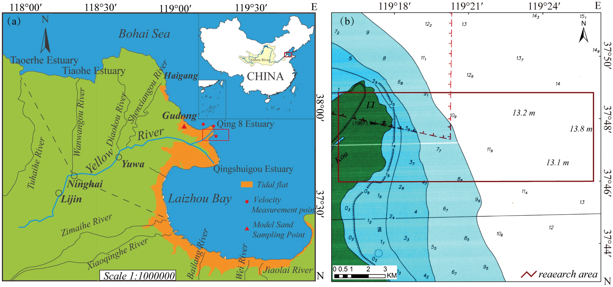
(a) Annual sediment load of the Yellow River; (b) Annual runoff of the Yellow River.
According to the 1950-2017 annual sediment load and runoff statistics of the Yellow River from Lijin Hydrological Station (Figure 2), the sediment load of the YR has declined annually since 1984. In 1984, the sediment load volume was 9.33×10⁸ t, whereas in 2017, it decreased to 0.08×10⁸ t, representing a reduction of 99.14%. Measured data indicate that the SSC near the YR estuary during the flood season in 1984 ranged from 2.13 to 14.9 kg/m³ (Zhou et al., 2007).
Figure 2
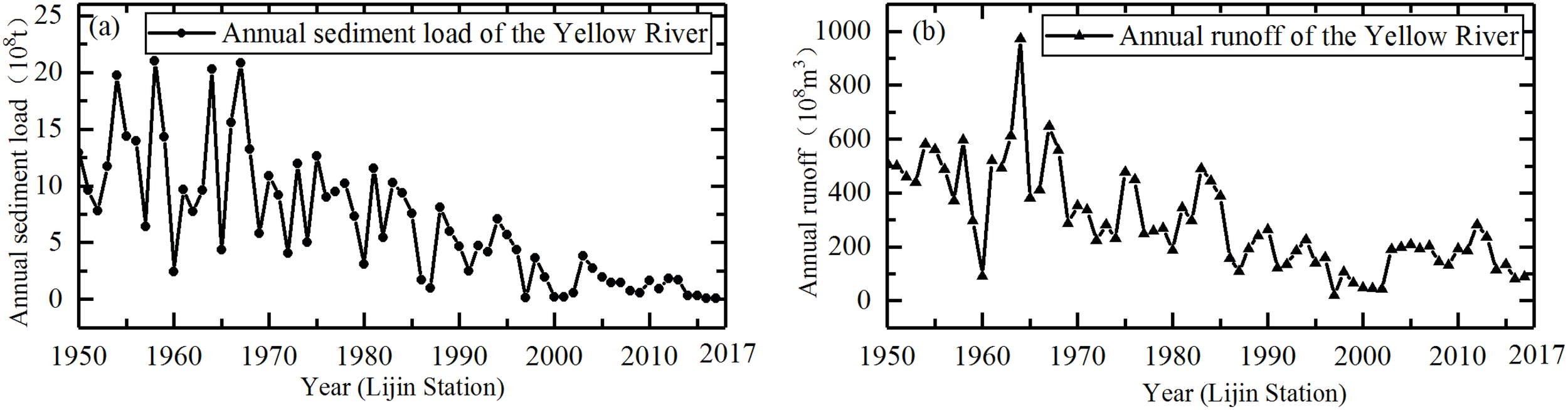
(a) Annual sediment load of the Yellow River; (b) Annual runoff of the Yellow River.
Waves near the YR Estuary exhibit seasonal characteristics, corresbasining to changes in wind direction. The predominant wave direction is NE, with a maximum wave height of 5.1 m and a maximum period of 8.2 s. The average tidal range in most sea areas of the YRD is 0.73-1.77 m, while near Qingshuigou, it is 1.1-1.5 m (Hu and Cao, 2003). The average high tide duration is 5 hours and 23 minutes, and the average low tide duration is 6 hours and 53 minutes. Measured data show that the velocity range of the YR estuary is 0.02-1.4 m/s (Xia et al., 1991).
Experimental design and research methods
A physical model experiment scales down the natural system to a laboratory scale according to the similarity criterion. It can then be used to simulate the movement and transformation patterns of natural materials. In this study, sediment movement includes both suspended and bedload sediment. During the experiment, tidal flat deformation is primarily driven by bed erosion. Wide tidal flats can be simulated using a perverted scale. Based on these considerations, this study employs a perverted scale, mobile bed, and full-sediment experiment to investigate the effects of reduced suspended sediment concentration on tidal flat morphology due to the combined influence of tidal currents, waves, and sediment transport in nearshore areas. According to the “Technical Regulations for Modeling Tidal Currents and Sediment in Coastal and Estuarine Areas,” the model variability can range from 3 to 10. Therefore, a model variability of 7.5 is used, with a vertical scale of λh = 100 and a horizontal scale of λl = 750.
The main similarity rules
According to the tidal current equation (Dou, 2001), we can obtain the velocity scale λu (Equation 1) and time scale λt (Equation 2) according to the water depth scale λh under the similar conditions of inertial force and gravity.
According to the linear wave theory (Hedges, 1976), we can determine the scaling value of the wave period λT (Equation 3). If the wave velocity of the model and the prototype are similar, the wave height scale λH (Equation 4) and the wavelength scale λL must be the same, calculated according to the water depth scale λh.
Wave breaking is influenced not only by water depth, wavelength, and wave height, but also by the slope of the tidal flat. Based on the relationship between wavelength, wave height, water depth, and slope (Hayashi et al., 1977), wave breaking is influenced by the slope when the prototype slope exceeds 1/50 (Equation 5). However, when the slope is less than 1/50, wave breaking is not affected by the slope. The slope of the YRD is relatively gentle, significantly less than 1/50, and therefore wave breaking is not influenced by the slope. Both the prototype and the model can achieve similarity in wave breaking. The equation for the allowable variability in the model is as follows:
where m represents the prototype slope, and the model variability is set to 7.5 in this study, which satisfies the requirements.
Based on the equations for suspended sediment transport and riverbed erosion and accretion (Dou et al., 1987), the scaling values for sediment settling velocity λω, (Equation 6) suspended sediment concentration λS*, (Equation 7) and suspended sediment movement time λts (Equation 8) can be derived as follows.
in this equation, λγ0 represents the scaling factor for the dry bulk density of sediment, λγs is the scaling factor for the particle density of the sediment, and λρ;s-ρ; is the scaling factor for the difference between the particle density and the water density.
Based on the equations for bed load transport and bed erosion and accretion (Dou, 2001), the scaling values for the bed load transport λN (Equation 9) and bed load movement time λts (Equation 10) can be derived.
After calculation, the model similarity scaling values are shown in Table 1.
Table 1
| Name | Symbol | Size | Name | Symbol | Size |
|---|---|---|---|---|---|
| Plane Vertical |
λl | 750 | Wave height and length | λH&λL | 100 |
| λh | 100 | Wave period | λT | 10 | |
| Velocity | λu | 10 | Sediment settling velocity | λω | 1.33 |
| Time | λt | 75 | SSC | λs* | 1 |
| Sediment erosion and accretion time | λts | 75 | Bed load transport | λN | 1000 |
The main similar scale.
The experimental device and sediment preparation
The experiment was conducted at the Coastal Engineering Laboratory of Ludong University, Yantai, China. The wave-current basin (Figure 3a) measures 27 m × 7 m × 1 m, while the tidal flat simulation area covers 7 m × 7 m× 0.2 m (slope 1:35). The experimental setup consists of four components: the tidal flat simulation area, the Water and Sand Uniform Mixing and Tidal Circulation device (Figure 3b), the Create Waves and Currents device (Figure 3c), and the Argus system. The Water and Sand Uniform Mixing and Tidal Circulation device has dimensions of 3 m × 1.5 m × 1.5 m and is constructed from welded stainless steel plates. It has a capacity of 6 m³ to hold muddy water. This device is used to prepare the muddy water and simulate both flood and ebb tides. The Create Waves and Currents device mainly consists of a wavemaker and a large number of nozzles, which generate waves and currents in the basin.
Figure 3
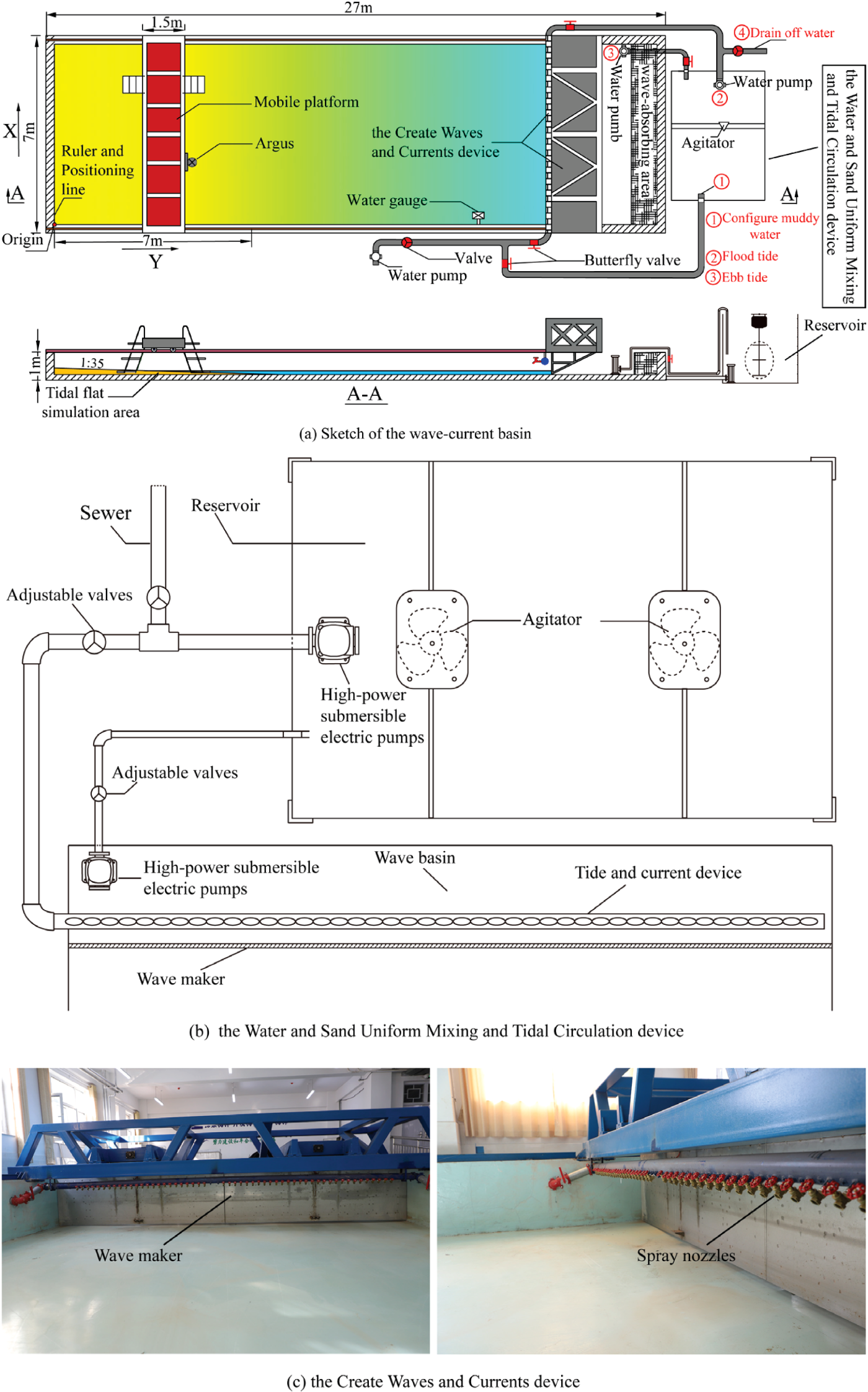
(a) Sketch of the wave-current basin; (b) the Water and Sand Uniform Mixing and Tidal Circulation device; (c) the Create Waves and Currents device.
Figures 3a, b illustrate the working principle of the Water and Sand Uniform Mixing and Tidal Circulation device. Assuming a still water level of 10 cm, a tidal range of 1 cm, and suspended sediment concentrations of 5 kg/m³, 2 kg/m³, and clear water, respectively, the process begins by injecting clear water into the wave basin until the still water level reaches 10 cm. Next, muddy water is prepared (indicated by red ① in Figure 3a). 4 m3 of clear water are added to the reservoir, and the agitators are activated. Then, 20 kg of dry sand is slowly added to the reservoir. Under sufficient mixing, the SSC in the reservoir is maintained at 5 kg/m³. The flood tide is simulated next (indicated by red ② in Figure 3a). A high-power pump is started, and the muddy water is continuously delivered to the wave basin through a nozzle array. The flow rate is adjusted by controlling the valve on the pipeline. When the water level rises by 1 cm, the pump is turned off. The ebb tide is then simulated (indicated by red ③ in Figure 3a). The pump in the wave basin is activated, and the muddy water is drawn back into the reservoir. Again, the flow rate is adjusted using the valve. When the water level decreases by 1 cm, the pump is turned off. After completing the tidal cycle, the water in the wave basin and reservoir is drained by activating pumps ② and ③ and opening valve④. The process for the “2 kg/m³ SSC” condition is similar. The “clear water” condition follows the same procedure, except that no sand is added to the reservoir.
The grain size of natural sediment in tidal flats exhibits distinct zonal distribution characteristics. As shown in Figure 1, during the ebb tide phase on September 15, 2018, at 4:30 PM, rectangular quadrats measuring 50 m in length and 2 m in width were established in the middle and upper sections of the tidal flat located south of Gudong (119.09°E, 37.84°N). A custom-made sampler with dimensions of 3 cm × 3 cm × 3 cm was used to randomly collect surface sediment to a depth of 2 cm from both quadrats. The samples were then transported to the laboratory for particle size analysis. For the experimental sand, surface sediment to a depth of 10 cm was collected using a soil shovel and placed into cement bags. A total of 400 bags were collected, with approximately 300 bags from the middle section of the tidal flat and 100 bags from the upper section. The total weight of the collected sediment was approximately 15 tons. The sediment from the middle section of the tidal flat was used as the bed load in the basin, while the sediment from the upper section was used as suspended sediment in the basin. In the laboratory, particle size analysis was performed using the Malvern Mastersizer 2000 laser diffraction particle size analyzer. According to the analysis results, the average grain size of the bed load ranged from 0.0378 to 0.0472 mm, with sand content ranging from 10.46% to 15.54%, silt content ranging from 84.46% to 88.01%, and clay content ranging from 0% to 1.69%. The average grain size of the suspended sediment ranged from 0.022 to 0.033 mm, with sand content ranging from 7.21% to 10.51%, silt content ranging from 88.01% to 92.76%, and clay content ranging from 0.04% to 3%.
All the sediment was naturally dried indoors and then crushed into powder using a roller. The natural density, dry density, saturated wet density, and porosity of the sediment were measured using the cutting ring method. Five measurements were taken, and the average value was calculated. The results showed that the natural density was 1510 kg/m³, the dry density was 890 kg/m³, the saturated wet density was 1750 kg/m³, and the porosity was 52.2%.
In the basin, slope lines with a ratio of 1:35 were marked every 2 m to indicate the gradient. Sand was then added to the basin, and a 2-meter-wide scraper was used along the slope lines to level the surface until the slope of the entire tidal flat was uniform (see Supplementary Figure 1a). The tidal flat was immersed in water for 12 hours to achieve full saturation. Afterward, sand was added along the slope lines, and the surface was leveled again using the scraper.
Experimental process
The experiment had five cases: 100% SSC, 65% SSC, 30% SSC, 15% SSC and clear water, which corresponded to suspended sand concentrations of 14.9 kg/m³, 9.7 kg/m³, 4.5 kg/m³, 2.2 kg/m³, and 0 kg/m³, respectively. It should be noted that the topography for each case was not reshaped to initial slope. This approach was adopted to simulate the linear superimposition effect of the reduced sediment input from the Yellow River on the evolution of the tidal flat in the real world. Each group underwent 36 tide cycles to simulate the 18-day dynamics of wave-current coupling in the prototype.
Due to the extremely gentle slope of the tidal flats in the Yellow River estuary, a slope of 1:35 was used to represent the gentle slope in the experimental setup, given the existing laboratory conditions. Based on the previously discussed marine dynamic environment of the Yellow River estuary and the similarity scaling factors provided in Table 1, the following model parameters were set: tidal range, wave height, flood duration, and ebb duration. As shown in Figure 4, the still water depth was 13.5 cm, and the tidal range was 1.5 cm. Specifically, the tide rises from 13.5 cm to 15 cm and falls from 15 cm to 13.5 cm. Consequently, the area from 0 cm to 176 cm is classified as the supratidal zone, from 176 cm to 227 cm as the intertidal zone, and from 227 cm to 700 cm as the subtidal zone. The flood tide lasts approximately 4 minutes and 18 seconds, while the ebb tide lasts approximately 5 minutes and 30 seconds. Regular waves were employed in the tests: incident wave height H = 0.05 m, and incident wave period T = 0.8 s.
Figure 4
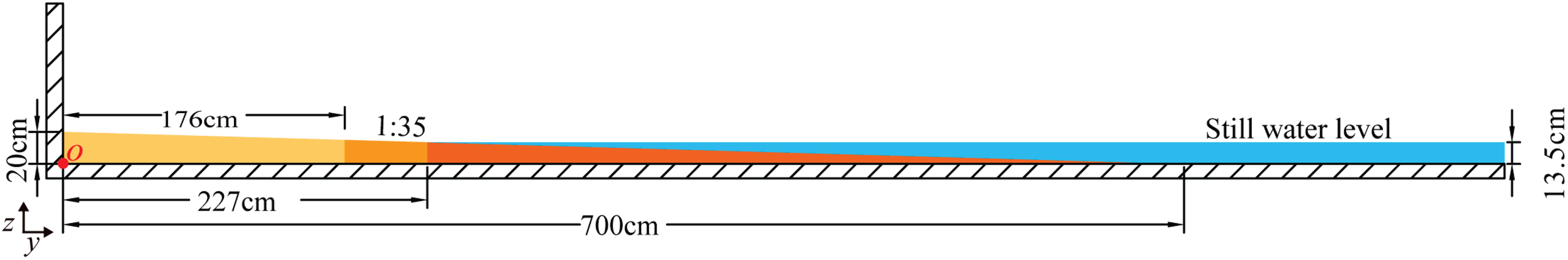
The schematic diagram of the tidal flat in the basin.
The experimental data collection consisted of four primary components:
-
Sediment concentration variation in the subtidal zone: Water samples were collected at five stages: at the beginning of the flood tide, the middle of the flood tide, the end of the flood tide, the middle of the ebb tide, and the end of the ebb tide, across the 10th, 20th, 30th, and 36th tidal cycles. A total of 80 muddy water samples (excluding clear water samples) were collected from the surface layer (2 cm) of the water at the subtidal zone (y = 500 cm) using bottles with a capacity of 500 ml. SSC was measured using the drying method.
-
Sand wave movement pattern and development mechanism: As shown in Supplementary Figure 1, the position, wave height, wavelength, wave form, and slope form of sand waves were recorded for different profiles under each case. The results are presented in Supplementary Figures 4–8.
-
Snapshots of the tidal flat: The Argus system, installed on a mobile platform, was used to capture photographs of each quadrat on the tidal flat. The photos are shown in Supplementary Figures 9–13. For specific quadrat (Nos. 1 to 9), the camera was placed at the following locations: x=116.5 cm, y=345 cm, z=129 cm; x=349 cm, y=345 cm, z=129 cm; x=582 cm, y=345 cm, z=129 cm; x=116.5 cm, y=578 cm, z=129 cm; x=349 cm, y=578 cm, z=129 cm; x=582 cm, y=578 cm, z=129 cm; x=116.5 cm, y=811 cm, z=129 cm; x=349 cm, y=811 cm, z=129 cm; x=349 cm, y=811 cm, z=129 cm.
-
Spatial distribution of erosion and accretion: Tidal flat elevations for each condition were manually measured at the sampling points shown in Supplementary Figure 2. The change in topography at each measurement location was determined by the elevation difference before and after wave-current action. Kriging interpolation was then applied to the elevation differences for spatial interpolation, in order to study the spatial distribution of erosion and deposition on the tidal flat.
Model validation
Hydrodynamic validation
An acoustic Doppler velocimeter (ADV) with 10 Hz sample rate was placed at the front edge of the tidal flat to measure the flow velocity. Based on the prototype velocity range of 0.02-1.4 m/s, the experimental basin should produce a velocity range of 0.2-14 cm/s. As shown in Supplementary Figure 3, the water velocity range for ebb tide is approximately 0.03-15.3 cm/s, while for flood tide it is 0.18-14.9 cm/s. These ranges satisfy the required specifications.
As shown in Figure 5a, a comparison is made between the observed and experimental tidal duration curves. The observed data were collected from the Kendong Tidal Station near the YRD during the spring tide on May 9, 2024. As indicated in the figure, the tidal processes of both the flood and ebb tides are consistent in duration. Regarding tidal heights, the errors in the high tides at hours 0, 12, and 24 are 8 cm, 19 cm, and 20 cm, respectively. The errors in the low tides at hours 7 and 19 are 17 cm and 28 cm. When converted to the model scale, the maximum tidal height error is 2.8 mm. The tidal pattern near the Yellow River Estuary is irregular semi-diurnal, with significant differences in the tidal range between the two high and low tides. However, the experimental device used to simulate tidal cycles can only produce regular flood and ebb tides. As a result, the errors in tidal heights are unavoidable. The Yellow River Estuary is a micro-tidal estuary, where tidal dynamics are relatively weak and tidal influence on sediment transport and scouring is minimal. Therefore, we consider the errors in tidal heights in this experiment to have a negligible effect on the development of tidal flats.
Figure 5
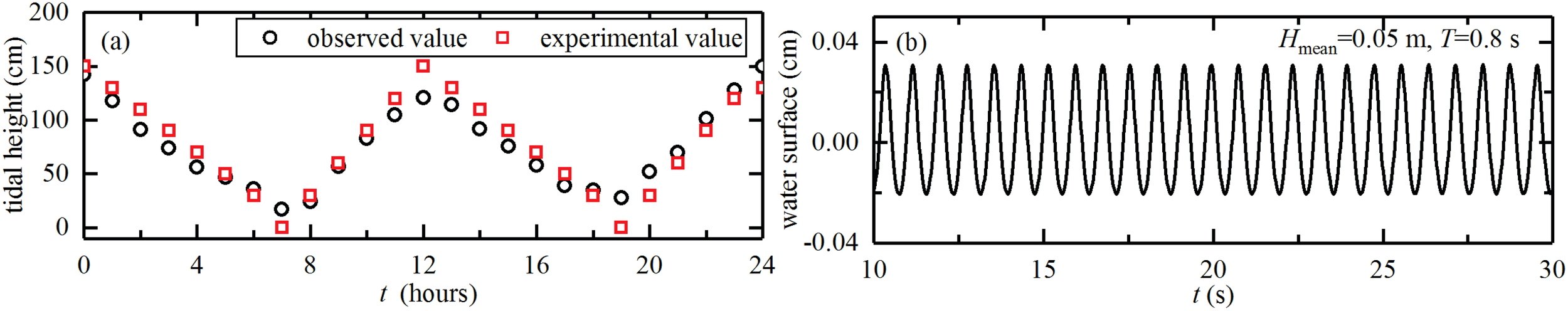
(a) Tide validation at the field scale; (b) wave boundary conditions in the experimental basin.
As shown in Figure 5b, the wave boundary conditions for the experimental basin are illustrated. When the basin is empty, the wave gauge is placed 20 cm in front of the wavemaker to measure the incident wave height and verify the stability of the wave form. The mean wave height (Hmean) and period (T) were calculated over 10 wave cycles. The results indicate a mean wave height of 0.05 m and a period of 0.8 s, with a stable wave form that meets the required wave conditions for the experiment.
Validation of sediment mobilization velocity
Using the sediment initial movement velocity equation for silt (Dou, 1999), the calculated initial movement velocity in the basin is 7.39 cm/s, indicating that the sediment is capable of mobilization.
Results
Variation of sediment concentration in the subtidal zone
In Figure 6, “10th” denotes the tenth tide cycle. The abbreviations BF, MF, EF, ME, and EE correspond to the beginning of the flood tide, the middle of the flood tide, the end of the flood tide, the middle of the ebb tide, and the end of the ebb tide, respectively. As shown in the figure, the higher the SSC at the experimental boundary, the SSC in the subtidal zone. For the boundary SSC of 100% to clear water, the corresponding average SSC in the subtidal zone were 0.97 kg/m³, 0.51 kg/m³, 0.29 kg/m³, and 0.13 kg/m³, respectively. The SSC in the subtidal zone was only 6.5%, 5.3%, 6.4%, and 6.0% of the boundary input SSC. This indicates that a large portion of the suspended sediment settles during transport from the offshore zone to the tidal flat, with only about 6% reaching the subtidal zone. Additionally, within a tidal cycle, the SSC in the subtidal zone fluctuates. The pattern can be summarized as follows: the SSC in the subtidal zone gradually increases during the flood tide and gradually decreases during the ebb tide.
Figure 6
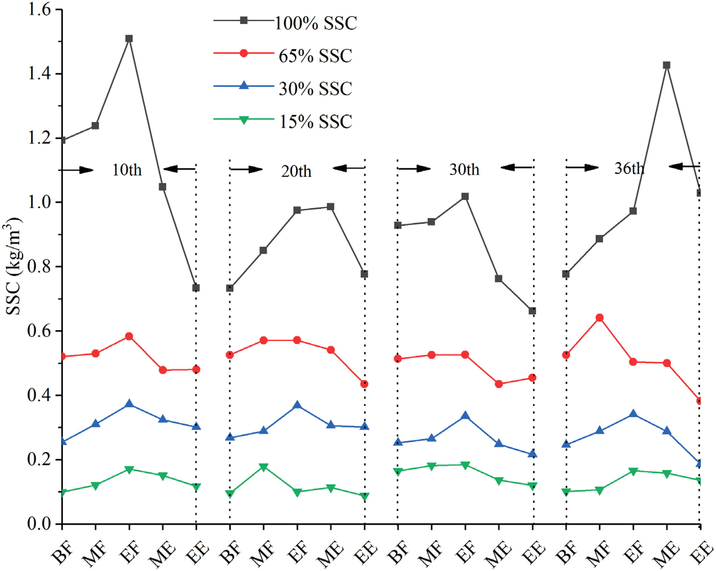
SSC in subtidal zone.
Although the SSC observed during the tidal cycle shows notable fluctuations, it is possible that the system may reach a dynamic equilibrium over longer time scales. This equilibrium could be influenced by factors such as sediment supply, tidal forces, and hydrodynamic conditions, leading to a more stable state of SSC in the subtidal zone. However, further long-term monitoring and analysis are necessary to confirm this hypothesis and accurately characterize the behavior of SSC over extended periods.
Sand wave movement pattern
Data on sand wave characteristics (Figure 7) were collected along different longitudinal profiles, ranging from x = 50 cm to x = 650 cm (Supplementary Figure 1). Supplementary Figures 4–8 present the statistical results of sand wave height, wavelength, angle, wave form, and slope form. The notation WF-SF represents wave form and slope form.
Figure 7
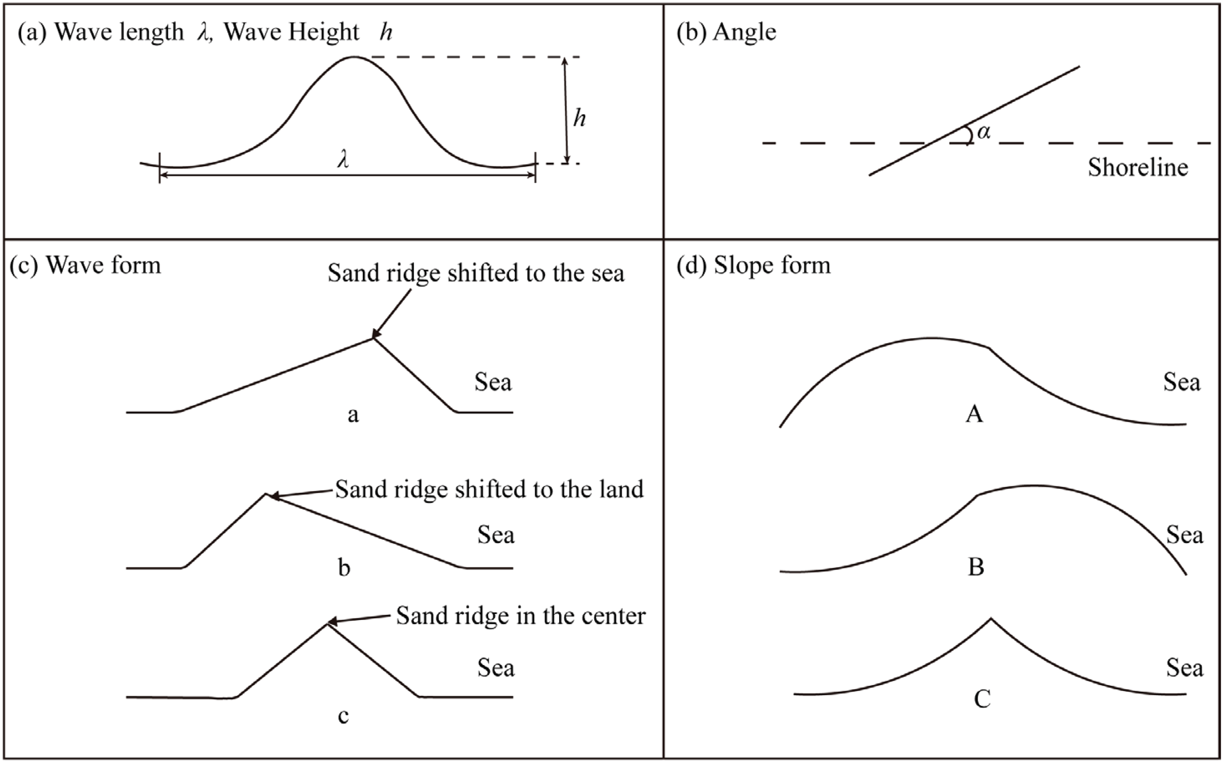
Sand wave characteristic diagram: (a) wave length and wave height; (b) angle; (c) wave form; (d) slope form.
The wave height, wavelength, wave form, and slope form of sand waves evolve as SSC decreases. However, the decrease in SSC has a relatively small effect on the angle of the sand waves. For instance, in the x = 50 cm profile (Supplementary Figures 4a–c – 8a–c), in the region where y > 600 cm, as SSC decreases, the sand wave height first decreases, then increases. The wavelength stabilizes around 2 cm, then decreases to 1 cm, and finally increases to around 3 cm. The wave form undergoes an a-c-a-c change, while the slope form shows a C-A-C-A pattern. However, the angle of the sand waves remains unchanged and is parallel to the shoreline. Under the same SSC condition, the statistical characteristics of sand waves differ significantly across profiles. For example, under 100% SSC (Supplementary Figure 4), the wave height increases progressively from land to sea at profiles x = 50 cm, x = 350 cm, x = 500 cm, and x = 650 cm, while the wave height at the x = 200 cm profile first increases and then decreases. Other statistical features also vary significantly across different profiles.
Supplementary Figure 4 presents the statistical results of sand wave characteristics under 100% SSC conditions. Except for the x = 200 cm profile, sand wave height generally increases from the intertidal zone toward the subtidal zone, with the maximum height occurring in the subtidal zone. The maximum sand wave heights at x = 50 cm, x = 350 cm, x = 500 cm, and x = 650 cm are 2.2 mm, 3.0 mm, 2.0 mm, and 2.1 mm, respectively. No consistent pattern was observed in wavelength variations across different profiles, with wave lengths ranging between 1.3 cm and 3.4 cm. In the subtidal zone, higher flow velocity and relatively stable hydrodynamic conditions facilitate sediment accumulation and redistribution, leading to the formation of higher sand waves. In contrast, the intertidal zone experiences periodic water level fluctuations and wave-induced scouring, which limit sediment stability and constrain sand wave height. The wavelength of sand waves is influenced by multiple factors, including water depth, flow velocity, and sediment grain size. Variations in local environmental conditions at different locations may result in random fluctuations in wavelength rather than a systematic trend. In the intertidal zone, sand waves form an angle with the shoreline, whereas in the subtidal zone, they are mostly parallel to the shoreline. Considerable differences were found in wave form and slope form across profiles. Generally, the c-A and b-C combinations dominate.
As shown in Supplementary Figures 5–7, the development process of sand waves can be summarized as follows: Sand wave height tends to be higher in the subtidal zone, with an average height of approximately 1 mm. No clear pattern is observed in wavelength variations across different profiles, with wave lengths fluctuating around 2 cm. In the intertidal zone, sand waves form an angle of approximately 50° with the shoreline, whereas in the subtidal zone, they are nearly parallel to the shoreline. As sediment concentration decreases, the proportion of sand waves exhibiting the “c-A” combination increases.
As illustrated in Supplementary Figure 8, after the clear-water experiment, sand wave height gradually increases from the intertidal to the subtidal zone, with higher sand waves observed further offshore, reaching a maximum height of approximately 3 mm. A similar trend is observed for wavelength, which increases from the intertidal to the subtidal zone, with a maximum value of approximately 2.7 cm. The orientation of sand waves follows the previously described pattern. After the clear-water experiment, all profiles were predominantly occupied by the “c-A” combination.
Tidal flat development responses to the decrease of SSC
As shown in Supplementary Figures 9–13, the first three samples (Nos. 1, 2, and 3) in each case exhibit flow marks that are nearly perpendicular to the shoreline. These marks have an average depth of approximately 0.5 mm and a width of around 0.5 mm. In contrast, the remaining samples are dominated by sand wave movement, with sand wave development varying as SSC decreases.
The tidal flat landforms observed after 36 tide cycles under 100% SSC are presented in Supplementary Figure 9. In this case, Nos. 4, 5, and 6 exhibit sand waves that are regularly distributed and parallel to the shoreline. Sand scales have developed in Nos. 7-3, 8-1, and 9-2. These sand scales result from the growth of sand waves as water flow intensity increases. In No. 7-1, both sand waves and flow marks coexist, indicating significant influence from tidal currents in this region. Supplementary Figure 10 displays results under the 65% SSC condition. The sand waves in Nos. 4 and 5 resemble those observed in the 100% SSC experiment. However, compared to the 100% SSC condition, Nos. 6, 7, 8, and 9 appear flatter, with fewer sand waves in certain area. Under the 30% SSC condition (Supplementary Figure 11), the density of sand wave increases in Nos. 4 and 5, and erosion begins to appear on the right side of No. 4. Nos. 6, 7, 8, and 9 are characterized by extensive flow marks oriented downslope, suggesting a strong influence of ebb currents. At 15% SSC (Supplementary Figure 12), the overall topography becomes flatter compared to the 30% SSC experiment, with continued erosion in Nos. 4 and 5. Unlike the 30% SSC condition, no flow marks are observed in Nos. 6, 7, 8, and 9. The clear water results (Supplementary Figure 13) show severe erosion in Nos. 4 and 5. Under these conditions, the density of sand waves is maximized, and sand scales are observed in No. 6-1. In the absence of suspended sediment, the water flow energy acts directly on the bed, leading to increased erosion intensity and a higher number of sand waves. In high-SSC environments, accretion rates are higher, facilitating the formation of flow marks and even stratified sediment layers along the flow direction. In contrast, in low-SSC environments, the accretion rate decreases, and wave-current interactions primarily shape sand waves rather than forming continuous flow marks on the surface.
Spatial distribution of erosion and accretion
The spatial distribution of erosion and accretion in tidal flat morphology, shown in Figure 8, was formed after a total of 180 tidal cycles. These cycles involved the coupled effects of waves and currents under conditions of 100% SSC (14.9 kg/m³), 65% SSC, 30% SSC, 15% SSC, and clear water, with each case running for 36 tidal cycles. As shown in Figure 8, the tidal flat at y (176-476 cm) was dominated by erosion, exhibiting a fan-shaped distribution, with erosion intensity increasing from the margins toward the center. The maximum erosion observed was approximately 0.7 cm, with an erosion rate of approximately 0.0039 mm/min. The tidal flat at y (476-700 cm) was predominantly characterized by accretion, with intensity increasing from land to sea. The maximum accretion was approximately 1.2 cm, and the accretion rate was approximately 0.0067 mm/min.
Figure 8
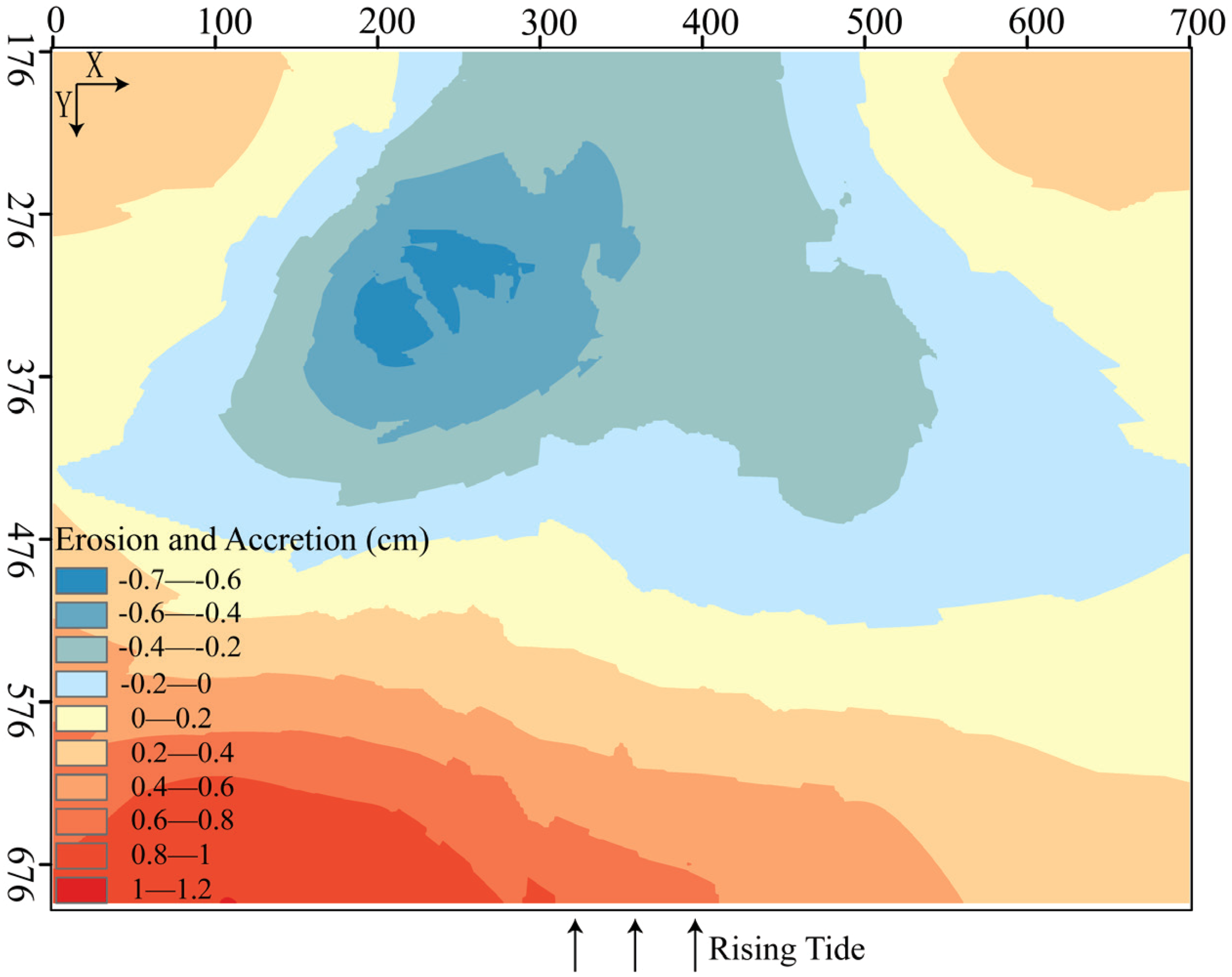
The spatial distribution of erosion and accretion after 180 tide cycles.
For the 100% SSC condition (Figure 9), the tidal flat was primarily characterized by accretion, with a small area of erosion. Accretion intensity increased gradually in a fan-shaped pattern, reaching its maximum at the basin margins. The maximum accretion, approximately 0.7 cm, occurred in the lower subtidal zone, with an accretion rate of approximately 0.194 mm/min. A small area of erosion, approximately 0.07 cm with an erosion rate of 0.002 mm/min, was observed at the center of the intertidal zone.
Figure 9
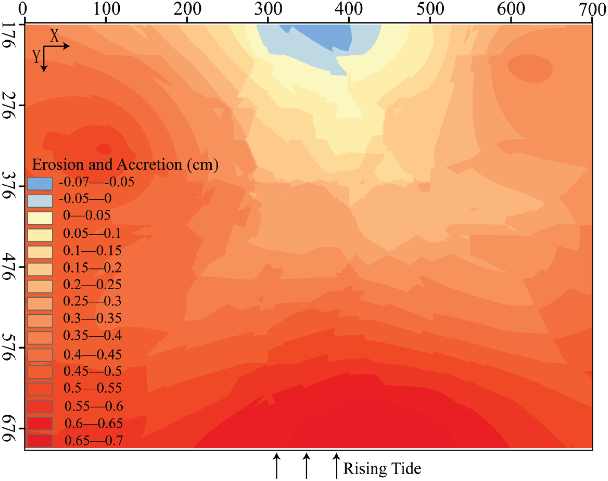
The spatial distribution of erosion and accretion for 100% SSC.
For the 65% SSC condition (Figure 10), both erosion and accretion were present on the tidal flat. Erosion intensity decreased from the center toward the margins (350-476 cm). The maximum erosion, approximately 0.33 cm, occurred in the middle of the subtidal zone, with an erosion rate of 0.009 mm/min. Accretion was primarily concentrated on the right side of the intertidal zone, with the maximum accretion, approximately 0.25 cm, and an accretion rate of 0.007 mm/min.
Figure 10
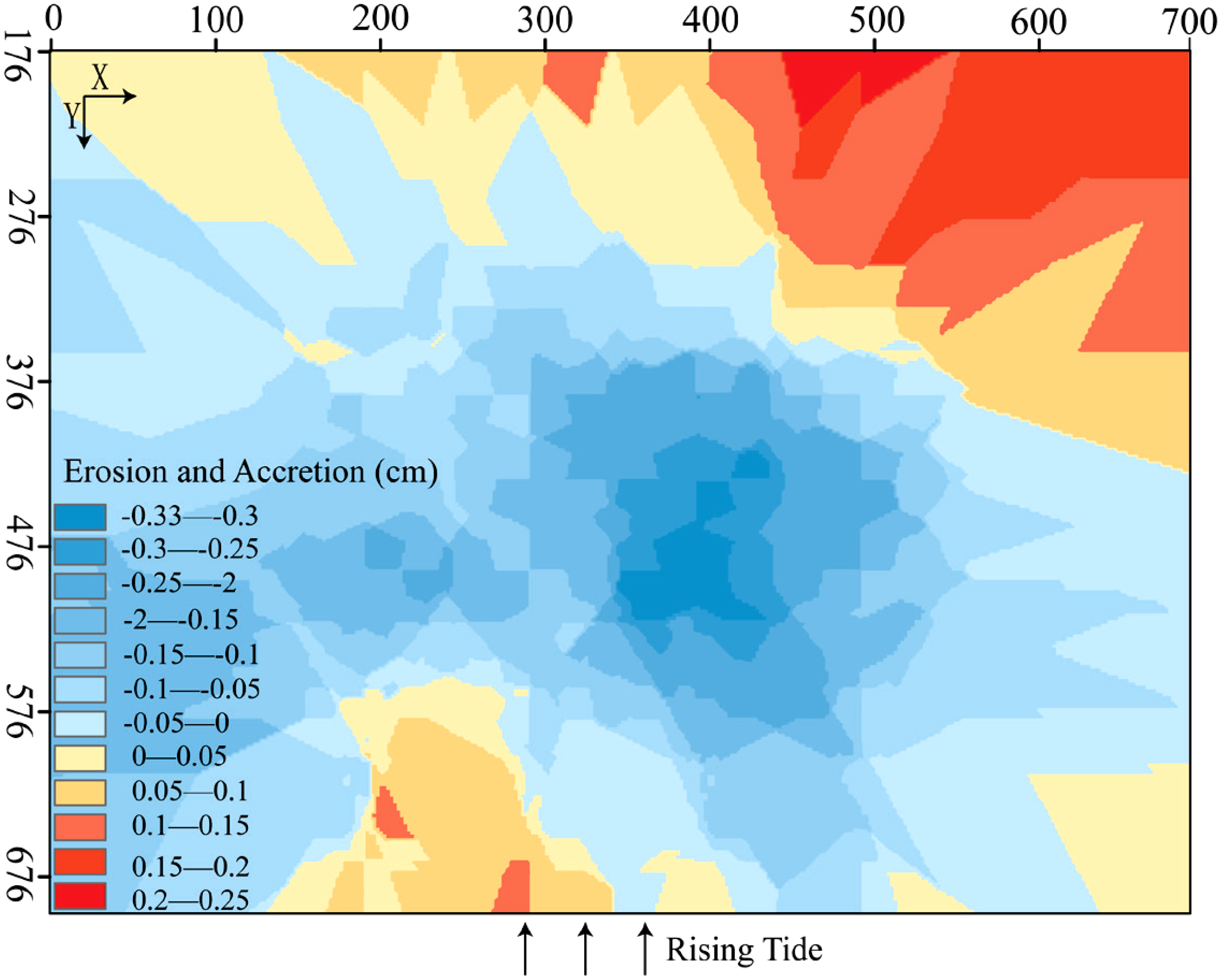
The spatial distribution of erosion and accretion for 65% SSC.
For the 30% SSC condition (Figure 11), the tidal flat was predominantly eroded, with some areas of accretion. The maximum erosion, approximately 0.3 cm, was observed in the lower subtidal zone, with an erosion rate of 0.009 mm/min. Accretion was concentrated on the right side of the intertidal zone, with the maximum accretion, approximately 0.1 cm, and an accretion rate of 0.003 mm/min.
Figure 11
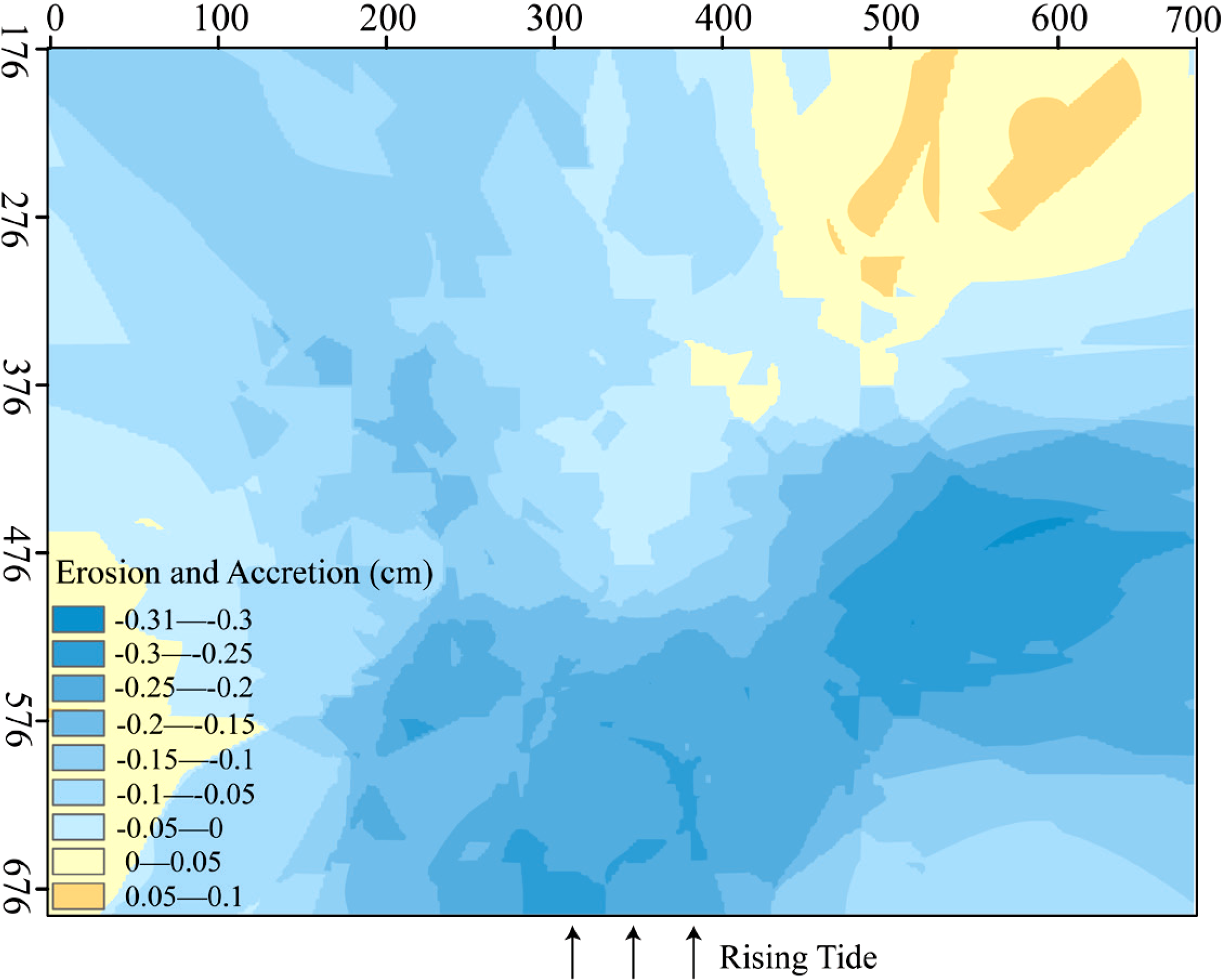
The spatial distribution of erosion and accretion for 30% SSC.
For the 15% SSC condition (Figure 12), the tidal flat was also dominated by erosion, with some accretion. The maximum erosion, approximately 0.2 cm, occurred in the subtidal zone, with an erosion intensity of 0.006 mm/min. Accretion was concentrated on the left side of the intertidal zone, with the maximum accretion, approximately 0.05 cm, and an accretion intensity of 0.001 mm/min.
Figure 12
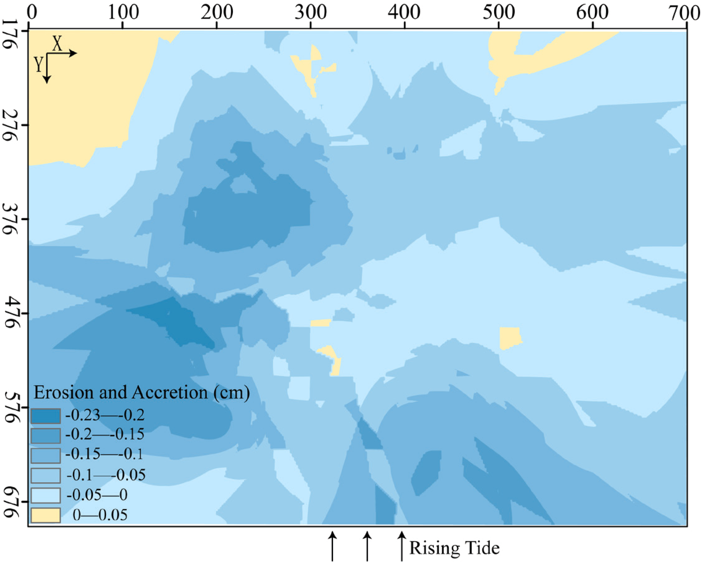
The spatial distribution of erosion and accretion for 15% SSC.
For the 0% SSC condition (Figure 13), the entire tidal flat was eroded. The maximum erosion was approximately 0.23 cm, with an erosion rate of 0.006 mm/min.
Figure 13
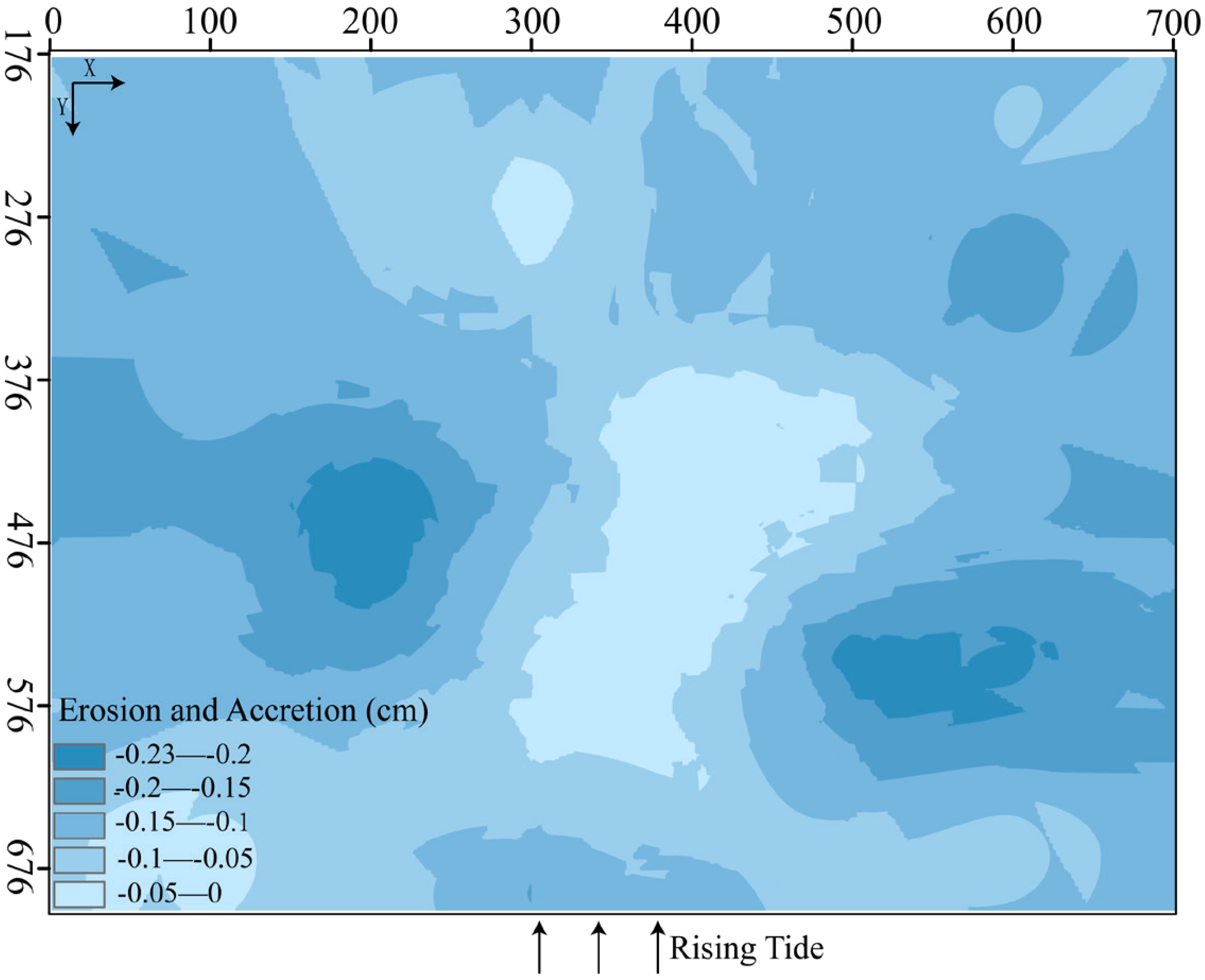
The spatial distribution of erosion and accretion for 0% SSC.
In general, both accretion and erosion coexist on the tidal flats. Taking the 7 m isobath as the boundary, the landward side was eroded, while the seaward side showed accretion. The closer a location is to the sea, the greater the accretion intensity. Specifically, for the 100% SSC condition, the entire tidal flat was dominated by accretion, with only a small area of erosion. For the 65% SSC condition, both erosion and accretion were present. For the 30% SSC and 15% SSC conditions, the tidal flat was predominantly eroded, with some areas of accretion. For the 0% SSC condition, the entire tidal flat was eroded.
As SSC was gradually reduced from 100% to 0%, the tidal flat underwent a transition from nearly complete accretion with minimal erosion to a state where both erosion and accretion coexisted, and eventually to a predominantly erosional state with minimal accretion. This progression suggests that the Yellow River Delta (YRD) may face an increased risk of erosion in the future.
Discussion
Figure A3 shows the custom-designed devices: (b) the Water and Sand Uniform Mixing and Tidal Circulation device, and (c) the Create Wave and Current device. The flow rate of the flooding tide is controlled by adjustable valves, with the spray nozzles closer to the valves generating slightly higher flow velocity and flow rate. Additionally, the ebb tide flow is generated by a high-power submersible pump and adjustable valves, located in the northwest corner of the wave basin, resulting in an asymmetric ebb flow. This uneven water flow distribution may lead to asymmetric sediment transport in the tidal flat, causing the distribution of sand waves and the extent of erosion and accretion to show a certain degree of asymmetry.
Due to limitations in sediment-carrying capacity, when SSC exceeds this capacity, a large amount of suspended sediment settles from the water onto the tidal flat. As a result, only about 6% of the SSC reaches the subtidal zone. Although a significant amount of suspended sediment does not enter the tidal flat, measured data show that a higher SSC input corresponds to a higher SSC in the subtidal zone. During the flood tide, the hydrodynamic force increases, enhancing the capacity for sediment transport. Most of the energy is used to resuspend the sediment, while the remaining energy scours the seabed and replenishes the sediment. Similarly, during the ebb tide, the hydrodynamic force weakens, reducing sediment transport capacity. The excess sediment gradually settles, causing a decrease in suspended sediment concentration over the course of the ebb tide.
Wave form c and slope form A were the most frequently observed in the results. In the model experiments, the hydrodynamic difference between flood and ebb tides was small, so waveform c dominated. However, some areas were influenced by either flood or ebb tide dominance, resulting in waveforms a or b.
As shown in Figure 14, on the seaward slope, flow velocity gradually increases, enhancing the scouring effect. The shear force from the water flow and the turbulence of the bottom bed cause sediment on the seaward slope to roll or jump along the slope surface and continue advancing with the flow, resulting in erosion. After the water flow crosses the crest, it enters the deceleration zone. As the flow speed slows, a vortex forms on the landward slope, where transported sediment accumulates. The principles of SF-B are similar to those of SF-A.
Figure 14
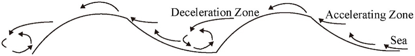
The trajectory of water points on the bed (Slope form A).
The results indicate that as SSC decreases, the erosion and accretion dynamics of tidal flats undergo significant changes. One crucial factor influencing these dynamics is the behavior of fine particles, particularly silt (80–90% of the sediment), which plays an important role in the stability and structure of the sediment bed. When suspended sediment concentrations are high, fine particles can settle into the interstitial spaces between coarser sand grains. This process, known as flocculation, enhances the cohesion of the sediment mixture by binding fine and coarse particles together. The increased cohesion reduces the bed’s erodibility, especially under low-flow conditions, which helps explain the observed accretion at high SSC.
Additionally, the cohesive nature of fine particles contributes to strengthening the sediment structure, particularly in deeper layers. As these fine particles accumulate in the sediment, they improve the overall resistance of the sediment bed to erosion, even under higher flow velocities. This phenomenon helps explain why sediment beds in environments with high SSC are more resistant to erosion, with the cohesive fine particles enhancing bed stability.
Our experimental results support these mechanisms, showing that high SSC conditions lead to greater accretion, likely due to the enhanced sediment cohesion from fine particles. These findings suggest that fine particles play a crucial role in controlling the stability and morphology of tidal flats, contributing to both accretion and resistance to erosion under varying SSC conditions.
However, it is important to note that due to the differences in scale between the experimental basin and natural environments, some scale effects may influence the sediment transport and settling behavior. The smaller dimensions of the experimental tank may lead to different flow characteristics and turbulence dynamics compared to real-world systems. Specifically, the settling velocity of sediment particles could differ because the experimental basin does not fully replicate the larger-scale turbulence and boundary layer effects found in natural tidal flats. These differences should be considered when extrapolating the results to natural systems. Nonetheless, the experiment still provides valuable insights into the general trends of sediment transport under varying SSC conditions and tidal forces. Additionally, it does not incorporate the specific geometry of the tidal flats, limiting its representation of the Yellow River Delta’s complex topography. Future studies will address this by incorporating tidal flat geometry and other factors to improve the model’s accuracy and representativeness.
Conclusion
-
Suspended sediment is primarily transported from the sea to tidal flats, with a significant portion settling along the way. As shown in Figure 6, the sediment concentration in the subtidal zone is typically less than 6% of the input SSC. Additionally, this study reveals that under consistent hydrodynamic conditions, a reduction in offshore sediment concentration results in lower SSC levels in the subtidal zone. The concentration of suspended sediment follows a distinct pattern, with a gradual increase during high tide and a corresponding decrease during low tide.
-
Under different SSC conditions, tidal flat morphology continuously evolves, with distinct morphological features appearing in various regions. The intertidal zone is primarily characterized by flow marks, while sand wave movement dominates the subtidal zone. The key factors influencing sand wave development are changes in SSC and water-sediment exchange. Within the same SSC condition, significant differences exist in the statistical characteristics and variation patterns of sand waves between different profiles. Additionally, under different SSC conditions, the development of sand waves at the same profile varies noticeably. Changes in SSC affect the number, wave height, wavelength, wave form, and slope form of sand waves, which in turn influence the development trends and distribution patterns of sand waves at each profile. However, the angle of the sand waves is less affected by SSC.
-
The spatial distribution of erosion and accretion on tidal flats, as illustrated in Figure 8, clearly demonstrates how SSC influences tidal flat morphology. The 7-meter isobath serves as a boundary where erosion occurs landward and accretion occurs seaward, with a stronger accretion intensity closer to the sea. For example, under 100% SSC conditions, the tidal flat is predominantly accretional, with minimal erosion. As SSC decreases to 65% and 30%, both erosion and accretion coexist, with a greater tendency toward erosion at lower SSC levels. At 15% SSC and clear water conditions, erosion dominates, leading to significant alterations in the tidal flat morphology. This trend suggests that as sediment transport in the Yellow River decreases, tidal flats may face an increasing risk of erosion in the future, a phenomenon that aligns with predictions made in previous studies (Cao et al., 2023).
-
The findings of this study suggest that the tidal flats in the Yellow River Delta (YRD) will continue to undergo changes as the SSC decreases. As indicated by the spatial distribution of erosion and accretion across various SSC conditions, the Yellow River Delta may transition to a more erosional state if current sediment transport trends persist. This trend is evident when comparing the experimental basin results (Figures 9–11) with historical data, which show a marked decline in sediment transport since 1984 (Lijin Hydrological Station, Figure 2). This study provides valuable insights into sediment transport mechanisms in tidal flats influenced by varying SSC conditions. The results suggest that the interplay between wave-current dynamics and sediment availability plays a crucial role in shaping tidal flat morphology.
Given that many tidal flats worldwide, including the Mississippi River Delta (USA), Ganges Delta (India), Amazon River Delta (Brazil), and Waikato River Estuary (New Zealand), are dominated by fine-grained sediments, the findings of this study may be applicable to similar environments. This is particularly relevant in the context of global tidal flat loss, with an estimated 16% decrease in tidal flat area worldwide over recent decades (Murray et al., 2019). The study’s findings underscore the importance of understanding the dynamics of sediment transport in these regions, where fine sediments play a dominant role. By linking the results of this study to broader global trends, we emphasize the significance of sediment management in tidal flats facing similar challenges globally. Future research could further explore the generalizability of these mechanisms across different tidal settings with varying hydrodynamic and sedimentary conditions.
Statements
Data availability statement
The raw data supporting the conclusions of this article will be made available by the authors, without undue reservation.
Author contributions
FY: Data curation, Formal analysis, Investigation, Visualization, Writing – original draft, Writing – review & editing. CZ: Conceptualization, Funding acquisition, Supervision, Writing – review & editing. QW: Funding acquisition, Project administration, Writing – review & editing. XL: Investigation, Supervision, Writing – review & editing. KF: Writing – review & editing.
Funding
The author(s) declare that financial support was received for the research and/or publication of this article. The authors would like to acknowledge the support from the National Natural Science Foundation of China (Grant No. U1706220, 52071057).
Conflict of interest
The authors declare that the research was conducted in the absence of any commercial or financial relationships that could be construed as a potential conflict of interest.
Generative AI statement
The author(s) declare that no Generative AI was used in the creation of this manuscript.
Publisher’s note
All claims expressed in this article are solely those of the authors and do not necessarily represent those of their affiliated organizations, or those of the publisher, the editors and the reviewers. Any product that may be evaluated in this article, or claim that may be made by its manufacturer, is not guaranteed or endorsed by the publisher.
Supplementary material
The Supplementary Material for this article can be found online at: https://www.frontiersin.org/articles/10.3389/fmars.2025.1546802/full#supplementary-material
Supplementary Figure 1The sketch of quadrat division and profile.
Supplementary Figure 2Elevation measurement points.
Supplementary Figure 3Flow velocity in experimental basin.
Supplementary Figure 4100% SSC sand wave movement.
Supplementary Figure 565% SSC sand wave movement.
Supplementary Figure 630% SSC sand wave movement.
Supplementary Figure 715% SSC sand wave movement.
Supplementary Figure 8Clear water sand wave movement.
Supplementary Figure 9Snapshot of tidal flat morphology (100% SSC).
Supplementary Figure 10Snapshot of tidal flat morphology (65% SSC).
Supplementary Figure 11Snapshot of tidal flat morphology (30% SSC).
Supplementary Figure 12Snapshot of tidal flat morphology (15% SSC).
Supplementary Figure 13Snapshot of tidal flat morphology (clear water).
References
1
Brunetta R. Duo E. Ciavola P. (2021). Evaluating short-term tidal flat evolution through UAV surveys: A case study in the Po Delta (Italy). Remote Sens.13, 2322. doi: 10.3390/rs13122322
2
Cahoon D. R. Perez B. C. Segura B. Lynch J. C. (2011). Elevation trends and shrink–swell response of wetland soils to flooding and drying. Estuar. Coast. Shelf Sci.91, 463–474. doi: 10.1016/j.ecss.2010.03.022
3
Cao J. Liu Q. Yu C. Chen Z. Dong X. Xu M. et al . (2024). Extracting waterline and inverting tidal flats topography based on Sentinel-2 remote sensing images: A case study of the northern part of the North Jiangsu radial sand ridges. Geomorphology461, 109323. doi: 10.1016/j.geomorph.2024.109323
4
Cao D. F. Shen Y. M. Su M. R. Yu C. X. (2019). Numerical simulation of hydrodynamic environment effects of the reclamation project of Nanhui tidal flat in Yangtze Estuary. J. Hydrodynamics31, 603–613. doi: 10.1007/s42241-019-0006-4
5
Cao Y. Wang Q. Zhan C. Li R. Qian Z. Wang L. et al . (2023). Evolution of tidal flats in the Yellow River Qingshuigou sub-delta: spatiotemporal analysis and mechanistic changes 1996-2021). Front. Mar. Sci.10, 1286188. doi: 10.3389/fmars.2023.1286188
6
Chen Y. Dong J. Xiao X. Zhang M. Tian B. Zhou Y. et al . (2016). Land claim and loss of tidal flats in the Yangtze Estuary. Sci. Rep.6, 1–10. doi: 10.1038/srep24018
7
Choi J. K. Ryu J. H. Lee Y. K. Yoo H. R. Woo H. J. Kim C. H. (2010). Quantitative estimation of intertidal sediment characteristics using remote sensing and gis. Estuar. Coast. Shelf Sci.88, 125–134. doi: 10.1016/j.ecss.2010.03.019
8
Dou G. R. (1999). Incipient motion of coarse and fine sediment. J. Sediment Res.6, 1–9. doi: 10.16239/j.cnki.0468-155x.1999.06.001 (in Chinese)
9
Dou G. R. (2001). Similarity theory of total sediment transport modeling for estuarine and coastal regions. Hydro-Science Eng.1, 1–12. doi: 10.16198/j.cnki.1009-640x.2001.01.001 (in Chinese)
10
Dou G. Zhao S. Huang Y. F. (1987). Study on two-dimensional total sediment transport mathematic model. Hydro-Science Eng.2, 1–11. doi: 10.16198/j.cnki.1009-640x.1987.02.001 (in Chinese)
11
Geng L. Gong Z. Zhou Z. Lanzoni S. D’Alpaos A. (2020). Assessing the relative contributions of the flood tide and the ebb tide to tidal channel network dynamics. Earth Surface Processes Landforms45, 237–250. doi: 10.1002/esp.v45.1
12
Gong Z. Lyu T. Y. Geng L. Zhou Z. Xu B. B. Zhang C. K. (2017). Mechanisms underlying the dynamic evolution of an open-coast tidal flat-creek system: I: physical model design and tidal creek morphology. Adv. Water Sci.28, 86–95. doi: 10.14042/j.cnki.32.1309.2017.01.010 (in Chinese)
13
Hayashi S. Tsuchida H. Noda S. (1977). Recent Revision of Design Standards on Seismic Effects for Port and Harbour Structures. In Wind and Seismic Effects: Proceedings of the 7th Joint Panel Conference of the US-Japan Cooperative Program in Natural Resources, May 20-23, 1975, Tokyo, Japan. US Department of Commerce, National Bureau of Standards. Vol. 470.
14
Hedges T. S. (1976). An empirical modification to linear wave theory. Proc. Institution Civil Engineers61, 575–579. doi: 10.1680/iicep.1976.3408
15
Hu C. H. Cao W. H. (2003). Variation, regulation and control of flow and sediment in the Yellow River Estuary: I. Mechanism of flow-sediment transport and evolution. J. Sediment Res.5, 1–8. doi: 10.16239/j.cnki.0468-155x.2003.05.001 (in Chinese)
16
Li L. Ren Y. Ye T. Wang X. H. Hu J. Xia Y. (2023). Positive feedback between the tidal flat variations and sediment dynamics: an example study in the macro-tidal turbid hangzhou bay. J. ournal Geophysical Research: Oceans128, e2022JC019414. doi: 10.1029/2022JC019414
17
Liu X. Qiao L. Zhong Y. Wan X. Xue W. Liu P. (2020). Pathways of suspended sediments transported from the Yellow River mouth to the Bohai Sea and Yellow Sea. Estuar. Coast. Shelf Sci.236, 106639. doi: 10.1016/j.ecss.2020.106639
18
Mei X. Leonardi N. Dai J. Wang J. (2023). Cellular automata to understand the prograding limit of deltaic tidal flat. Eng. Appl. Comput. Fluid Mechanics17, 2234038. doi: 10.1080/19942060.2023.2234038
19
Murray N. J. Phinn S. R. DeWitt M. Ferrari R. Johnston R. Lyons M. B. et al . (2019). The global distribution and trajectory of tidal flats. Nature565, 222–225. doi: 10.1038/s41586-018-0805-8
20
Prior D. B. Yang Z. S. Bornhold B. D. Keller G. H. Lu N. Z. Wiseman W. J. et al . (1986). Active slope failure, sediment collapse, and silt flows on the modern subaqueous Huanghe (Yellow River) delta. Geomarine Lett.6, 85–95. doi: 10.1007/BF02281644
21
Saito Y. Wei H. Zhou Y. Nishimura A. Sato Y. Yokota S. (2000). Delta progradation and chenier formation in the Huanghe (Yellow River) delta, China. J. Asian Earth Sci.18, 489–497. doi: 10.1016/S1367-9120(99)00080-2
22
Shen F. Ren Y. Li L. He Z. (2023). Vertical sediment distribution mechanism in tidal flats-A case study in Zhoushan Archipelago. Estuarine Coast. Shelf Sci.293, 108503. doi: 10.1016/j.ecss.2023.108503
23
Siegle E. Dottori M. Villamarin B. C. (2018). Hydrodynamics of a subtropical tidal flat: Araçá Bay, Brazil. Ocean Coast. Manage.164, 4–13. doi: 10.1016/j.ocecoaman.2017.11.003
24
Stefanon L. Carniello L. D’Alpaos A. Rinaldo A. (2012). Signatures of sea level changes on tidal geomorphology: Experiments on network incision and retreat. Geogr. Res. Lett.39, 85–91. doi: 10.1029/2012GL051953
25
Tseng K. H. Kuo C. Lin T. H. Huang Z. Lin Y. Liao W. H. et al . (2017). Reconstruction of time-varying tidal flat topography using optical remote sensing imageries. Isprs J. Photogrammetry Remote Sens.131, 92–103. doi: 10.1016/j.isprsjprs.2017.07.008
26
Vlaswinkel B. Cantelli A. (2011). Geometric characteristics and evolution of a tidal channel network in experimental setting. Earth Surface Processes Landforms36, 739–752. doi: 10.1002/esp.v36.6
27
Wang H. J. Bi N. S. Saito Y. Wang Y. Sun X. Zhang J. et al . (2010). Recent changes in sediment delivery by the Huanghe (Yellow River) to the sea: causes and environmental implications in its estuary. J. Hydrology391, 302–313. doi: 10.1016/j.jhydrol.2010.07.030
28
Wang W. H. Gao S. Xu Y. P. Y. Xu Q. L. Yu Q. Zhao Y.Y (2014). Numerical experiments for the characteristic deposition rates over the tidal flat, central Jiangsu coast. J. Nanjing Univ. (Natural Sciences)50, 656–665. doi: 10.13232/j.cnki.jnju.2014.05.014 (in Chinese).
29
Wang H. J. Wu X. Bi N. S. Li S. Yuan P. Wang A. et al . (2017). Impacts of the dam-orientated water-sediment regulation scheme on the lower reaches and delta of the Yellow River (Huanghe): A review. Global Planetary Change157, 93–113. doi: 10.1016/j.gloplacha.2017.08.005
30
Xia D. X. Wang W. H. Liu C. X. (1991). Gulf of China (Volume 3: northern and eastern bays of shandong peninsula) (Beijing: Ocean Press), 105–107.
31
Yang Z. Ji Y. Bi N. Lei K. Wang H. (2011). Sediment transport off the Huanghe (Yellow River) delta and in the adjacent Bohai Sea in winter and seasonal comparison. Estuarine. Coast. Shelf Sci.93, 173–181. doi: 10.1016/j.ecss.2010.06.005
32
Zhang R. Chen Y. Chen P. Zhou X. Wu B. Chen K. et al . (2023). Impacts of tidal flat reclamation on suspended sediment dynamics in the tidal-dominated Wenzhou Coast, China. Front. Mar. Sci.10, 1097177. doi: 10.3389/fmars.2023.1097177
33
Zhang Q. Gong Z. Zhang C. Lacy J. Jaffe B. Xu B. et al . (2021). The role of surges during periods of very shallow water on sediment transport over tidal flats. Front. Mar. Sci.8, 599799. doi: 10.3389/fmars.2021.599799
34
Zhao B. Liu Y. Wang L. Liu Y. Sun C. Fagherazzi S. (2022). Stability evaluation of tidal flats based on time-series satellite images: A case study of the Jiangsu central coast, China. Estuarine Coast. Shelf Sci.264, 107697. doi: 10.1016/j.ecss.2021.107697
35
Zhou L. Y. Li A. L. Gong S. Y. Liu Y. Zhao D. B. Wen G. T. (2007). Spatial distribution and grain-size characteristics of suspended matters in surface water of yellow river mouth. Mar. Geology Quaternary Geology27, 33–38. doi: 10.16562/j.cnki.0256-1492.2007.05.014 (in Chinese)
Summary
Keywords
Yellow River Delta (YRD), suspended sediment concentration (SSC), tidal flat, co-action of waves and currents, physical model
Citation
Yi F, Zhan C, Wang Q, Li X and Fang K (2025) Physical study of the response of tidal flat development to the reduction in the input of Yellow River sediment into the sea. Front. Mar. Sci. 12:1546802. doi: 10.3389/fmars.2025.1546802
Received
17 December 2024
Accepted
24 March 2025
Published
10 April 2025
Volume
12 - 2025
Edited by
Juan Jose Munoz-Perez, University of Cádiz, Spain
Reviewed by
Jian Zhou, Hohai University, China
Elena Alekseenko, Université du Littoral Côte d’Opale, France
Updates
Copyright
© 2025 Yi, Zhan, Wang, Li and Fang.
This is an open-access article distributed under the terms of the Creative Commons Attribution License (CC BY). The use, distribution or reproduction in other forums is permitted, provided the original author(s) and the copyright owner(s) are credited and that the original publication in this journal is cited, in accordance with accepted academic practice. No use, distribution or reproduction is permitted which does not comply with these terms.
*Correspondence: Chao Zhan, zhanchaolddx@126.com
Disclaimer
All claims expressed in this article are solely those of the authors and do not necessarily represent those of their affiliated organizations, or those of the publisher, the editors and the reviewers. Any product that may be evaluated in this article or claim that may be made by its manufacturer is not guaranteed or endorsed by the publisher.