A multi-dimensional data-driven ship roll prediction model based on VMD-PCA and IDBO-TCN-BiGRU-Attention

Introduction: The motion of a ship at sea is complex. This motion is affected by environmental factors such as wind, waves, and currents. These factors cause the ship’s movement to be nonlinear, dynamic, and uncertain. Such complex motion can impact the ship’s performance and pose a safety risk. This has become an urgent problem in maritime safety. This study aimed to improve the prediction of a ship’s roll motion with high accuracy. As such, the study proposes a combined prediction model. This model integrates data decomposition, dimensionality reduction, deep learning, and optimization techniques.

Methods: The model uses the variational mode decomposition (VMD) method to break down the ship’s roll motion data into components at different scales. This improves the smoothness of the data. Principal component analysis (PCA) is applied to reduce the dimensionality of the decomposed components. This step helps remove noise and redundant features that could affect the prediction results. The core of the model combines temporal convolutional networks (TCNs) and bidirectional gated recurrent units (BiGRUs). These deep learning techniques enable the model to extract both spatial features and temporal dependencies from the data. An attention mechanism is added to focus on the most important features,improving the prediction accuracy of the model. Finally,the improved dung beetle optimization (IDBO) algorithm is used to optimize the hyper-parameters of the model. This step further enhances the model performance.

Results: Simulation experiments were conducted using full-scale data from the Yukun ship. The results show that the proposed prediction model has a root mean square error reduction of about 78.25% and an increase of about 65.63% reliability compared with TCN.

Discussion: The model outperforms traditional methods in terms of accuracy and stability. This demonstrates its potential for improving the prediction of ship motion an attitude.

1 Introduction

Ships play a very important role in the foreign trade of countries worldwide. Therefore, the safety of ship navigation has always been the focus of research by scholars in the field of marine engineering. When faced with a complex maritime environment made up of a combination of wind, waves, currents, and other factors, a ship will produce six degrees of freedom motions such as roll, pitch, and heave, among others. These oscillatory motions combine with each other to form a complex uncertain motion with nonlinear, non-stationary, and time-varying dynamics. Of these, the roll motion has great influence on the ship’s motion attitude, which poses a serious challenge to the maneuverability of the ship during sea operations and the safety of the takeoff and landing of the aircraft on board (Cheng et al., 2019; Huang et al., 2014; Fossen, 2011). Therefore, by grasping the ship roll motion state in a future period of time, the ship’s motion attitude can be adjusted in advance so that the ship can maintain a relatively stable motion attitude, which can improve the safety and efficiency of its maritime operation (Takami et al., 2021; Peng, 2023). At the same time, as the main method of maritime management is also carried out through the boat, the degree of swaying of the law enforcement vessel can be reduced if we can accurately forecast the angle of the ship roll motion. This can effectively reduce the fatigue of the managers and further improve the efficiency and safety of maritime management, which has a very important significance in the study of ship roll prediction in the field of engineering.

Researchers and scholars began the study of the accurate prediction of a ship’s motion attitude very early on. Limited by the development of computing equipment, the study of a ship’s motion attitude is based on traditional statistical analysis of a class of methods. There is also the use of hydrodynamic analysis with the Kalman filtering method (Kaplan, 1969; Triantafyllou and Athans, 1981). However, this method cannot meet the time-varying characteristics of a ship’s motion attitude in the complex ocean. Moreover, it is difficult to achieve a stable and accurate prediction of a ship’s motion attitude. Therefore, it is obvious that this method cannot be realized for engineering applications.

Later, it was found that the use of the ship’s historical motion attitude data to establish a time series model can avoid solving complex ship state equations and response functions. Firstly, it is assumed that the ship’s motion attitude data at sea are a smooth time series, so that an autoregressive (AR) model (Jiang et al., 2020) and a moving average autoregressive (ARMA) model (Broome and Hall, 1998; Moon et al., 2021) can be used for short-term forecasting of a ship’s motion attitude. Under certain conditions, integrating the moving average autoregressive model (ARIMA) (Wang et al., 2021; Zafeiraki, 2022) has shown a stronger performance. These models have the advantages of simple parameter calculations and relatively small computations, but these presuppose that the time series is characterized by smoothness and conformity to normal distribution. However, ships move in complex marine environments and their data are characterized by complexity, nonlinearity, and highly time-varying characteristics. Hence, the prediction accuracy using these models is low and cannot be applied in scenarios of ship motion forecasting.

Breakthroughs in high-performance computing equipment have made machine learning available for practical applications in many fields. Due to its powerful nonlinear approximation capability, machine learning can be used for the accurate forecasting of nonlinear, non-smooth stochastic time series. Extreme learning machines (ELMs) have been proposed for the roll prediction of ships and for very short-term wind speed prediction (Guan et al., 2018; Wang et al., 2018). One drawback faced by ELMs in both applications is that, if the inputs are not reasonable, the prediction results will be poor. In long-time series prediction, what is often used is the support vector regression (SVR) model, which is a variant of the support vector machine (SVM) when applied to regression tasks (Bo and Shi, 2013; Li et al., 2016). Radial basis function (RBF) networks have also been utilized in ship motion time series prediction (Yin et al., 2018). Recurrent neural networks (RNNs) are constructed models dedicated to dealing with time series problems and have performed very well when facing this class of problems (Ni and Ma, 2020; Zhang et al., 2019). However, RNNs run the risk of gradient vanishing and explosion when dealing with longer time series. Therefore, subsequent long short-term memory (LSTM) and gated neural networks (gated recurrent units, GRUs) have emerged to compensate for this shortcoming, which is realized by adding three special gates: input, output, and forgetting (Zhang et al., 2021; Su et al., 2020). Although a lot of effort has been invested in the development of such neural network algorithms to deal with some complex, strongly nonlinear time series data, such as the ship motion attitude data, there are still problems with regard to poor prediction accuracy and unstable prediction results. Therefore, researchers began to turn their attention to hybrid prediction.

A hybrid prediction model is an integrated model composed of different models to achieve a common prediction. Gao et al. (2023) proposed a ship motion attitude prediction model by combining the adaptive discrete wavelet transform (ADWT) algorithm and the spatiotemporal residual recurrent neural network (RRNN), which can use the ADWT to process the input data and then combine with the characteristic of RRNN of being able to change the structure and parameters to effectively improve the prediction accuracy. Zhou et al. (2023) first used variational modal decomposition (VMD) to decompose the input data and then to input the decomposed data into GRU for prediction. At the same time, the binary system optimization (BSO) algorithm was used to optimize the GRU, which also made use of the advantages of different algorithms to complement each other and improve the accuracy of the model prediction results. Of course, there are many other such hybrid forecasting models (Zhang D. et al., 2023; Geng et al., 2024; Zhang et al., 2024; Xu and Yin, 2024), and the selection of appropriate algorithms for the construction of the hybrid forecasting model is extremely crucial for the prediction results.

As ship transverse motion data have both temporal dependence and spatial correlation, in order to obtain the laws between them in ship transverse motion, most of the hybrid prediction methods that combined convolutional neural network (CNN) and RNN have been previously used (Li et al., 2024; Agga et al., 2022; Cui et al., 2024). However, this also made the whole model more complicated, and the results were not too good. Therefore, temporal convolutional networks (TCNs) were developed (Bai et al., 2018), which combine the performance of both, with a fast learning speed. At the same time, it can obtain the temporal relationships in the sequences very well. One of the major challenges of a long time series is the huge amount of data involved. In order to facilitate the model focusing on learning the data with higher importance and avoiding the impact of less important features, an attention mechanism that focuses on feature selection learning was proposed (Bhunia et al., 2019). One of the difficulties of machine learning is parameter tuning. As such, there are many hybrid prediction methods that incorporate intelligent optimization algorithms into the model and use these optimization algorithms to optimize the hyper-parameters (Zhang B. et al., 2023). Fu et al. (2024) proposed the dung beetle optimization (DBO) algorithm to optimize the TCN. The results showed that this model has high accuracy and generalization. The performance of DBO is more stable in most cases, and its convergence is faster compared with other swarm intelligence optimization algorithms. Therefore, its use as a basis for improvement is a more appropriate direction.

Due to the complexity, nonlinearity, and instability of the ship roll data, in order to improve the prediction accuracy of the ship roll motion, a multidimensional data-driven ship transverse motion prediction model based on VMD–principal component analysis (PCA) and improved dung beetle optimization (IDBO)–TCN–bidirectional gated recurrent unit (BiGRU)–Attention is proposed in this paper. Firstly, VMD can decompose the time series ship motion data and remove noise according to its characteristics. The processed data can then effectively reduce its non-stationarity so that the input data have certain characteristics of smooth randomness, which improves the accuracy of data prediction. Secondly, the PCA method was used to extract the important sequences of the time series data after decomposition of the ship’s motion so as to improve the influence of the important data and to reduce the influence of the secondary data on the prediction results. Thirdly, a forecasting model using the IDBO algorithm combined with the attention mechanism optimized over time CNN and GRU was used for forecasting. The proposed hybrid model can improve the accuracy and stability of the ship’s motion attitude prediction. After verification of the real ship data of the Yukun ship, the school training ship of Dalian Maritime University, accurate and real-time prediction of the ship motion attitude is achieved, which improves the safety of ship navigation and provides certain support for the improvement of comfort in the process of maritime management, as well as improving the efficiency and safety in maritime management.

2 Methods

This section introduces the various modules of the hybrid forecasting model for ship roll motion, mainly including the VMD and PCA algorithms in the data pre-processing, the time CNN, the bidirectional gated neural network unit, and the self-attention mechanism in the combined forecasting model, as well as the mechanism of the IDBO algorithm with the hyper-parameter optimization strategy.

2.1 Variational modal decomposition algorithm

Due to empirical modal decomposition (EMD) suffering from endpoint effects and modal component aliasing, Dragomiretskiy and Zosso (2014) proposed variational modal decomposition (VMD). VMD is a non-recursive model that searches for the optimal solution of the variational model in each iteration in order to determine the center frequency of the components of each decomposition and the bandwidth (Liu et al., 2024). As it has very strict constraints, it decomposes the modal components to obtain the minimum sum of the bandwidth of the center frequency, and the original signal can be obtained after all modal components are superimposed.

Its solution process is as follows:

After inputting the ship roll data sequence $A(t)$, in order to make the decomposed individual k sequence satisfy the constraints, then the constrained variational model of the VMD is:

$\begin{array}{ll}\begin{array}{l}\underset{(u_k,{\omega }_k)}{min}\left\{{{\displaystyle {\sum }_k{\Vert }^{{\partial }_t}\left[\left(\delta (t)+\frac{j}{\pi t}\right)\ast u_k(t)\right]e^{j^{{\omega }_{k}t}}\Vert }}_2^2\right\}\\ s.t.\sum _k{u}_k{=}^{A(t)}\end{array}& (1)\end{array}$

In Equation 1, $u_k$ and ${\omega }_k$ are the k modal component and the center frequency, respectively. ${\partial }_t$ is the partial derivative of $t$ With respect to $\delta (t)$ is the Dirac distribution function, and ‘ $*$‘ denotes a convolution operation.

In order to solve the above constrained variational model, the augmented Lagrangian function is introduced. The Equation 2 can be obtained using the quadratic penalty factor and the Lagrangian multiplier:

$\begin{array}{ll}\begin{array}{l}L(\left\{u_k\right\},\left\{{\omega }_k\right\},\lambda )=\alpha \sum _k{{\Vert }^{{\partial }_t}\left[\left(\delta (t)+\frac{j}{\pi t}\right)\ast u_k(t)\right]e^{-j^{{\omega }_{k_t}}}\Vert }_2^2\\ +{{\Vert }^{A(t)}-\sum _k{u}_k(t)\Vert }_2^2+\langle \lambda (t){,}^{A(t)}-\sum _k{u}_k(t)\rangle \end{array}& (2)\end{array}$

$\text{α}$ is the penalty factor; $\text{λ}$ is the Lagrange multiplier; and $\langle \rangle$ is the inner product operator. Based on this unconstrained variational model, the modal component $u_k$ and the Lagrange multiplier ${\omega }_k$ can be obtained by using the alternating multiplier method (ADMM), which was calculated using the Equations 3-4:

$\begin{array}{ll}{\widehat{u}}_k^{n+1}(\omega )=\frac{{\widehat{A}}_{(\omega )-{\sum }_{i\ne k}{\widehat{u}}_i(\omega )+\widehat{\lambda }(\omega )/2}}{1+2\alpha {(\omega -{\omega }_k)}^2}& (3)\end{array}$

$\begin{array}{ll}{\omega }_k^{n+1}=\frac{{\int }_0^{\infty }\omega \left|{\widehat{u}}_k{(\omega )}^2\right|d\omega }{{\int }_0^{\infty }\left|{\widehat{u}}_k{(\omega )}^2\right|d\omega }& (4)\end{array}$

Here, n represents the number of iterations. The above formula was calculated by iteration to obtain the optimal solution.

When applying the VMD for data preprocessing, the number of modal components (k value) and the penalty coefficient (α value) are the two key parameters to be set. Of these, the choice of the number of modal components directly affects the decomposition effect: if the k value is too small, it will lead to insufficient modal components and the phenomenon of modal aliasing; if the k value is too large, it may produce spurious components, which will reduce the reliability of the decomposition results. The penalty coefficient, on the other hand, determines the bandwidth characteristics of each modal function, and its value affects the frequency resolution ability of the modal components. Therefore, a reasonable determination of the values of k and α is a prerequisite to ensuring the effectiveness of the VMD decomposition. In practical applications, parameter optimization can be carried out using the enumeration method, guided by auxiliary algorithms such as the principle of crag maximum and the principle of energy difference or combined with intelligent optimization algorithms to achieve automatic parameter optimization.

The selection of the fitness function is an important factor that affects the accuracy and efficiency of VMD. Currently, the commonly used fitness functions mainly include the following four categories: minimum envelope entropy, minimum information entropy, minimum arrangement entropy, and minimum sample entropy.

$\begin{array}{ll}\begin{array}{l}{E}_p=-{\displaystyle {\sum }_{j=1}^N{p}_{j}lg{p}_j}\hfill \\ p_j=a(j)/{\displaystyle {\sum }_{j=1}^{N}a(j)}\hfill \end{array}\}& (5)\end{array}$

$\begin{array}{ll}H(x)=-{\displaystyle {\sum }_{i=1}^N{p}_{i}lg{p}_i}& (6)\end{array}$

$\begin{array}{ll}H=\frac{\left(-{\sum }_{i=1}^k{P}_i·lg(P_i)\right)}{lg(m!)}& (7)\end{array}$

$\begin{array}{ll}SampEn(m,r,N)=-ln\left[\frac{A^m(r)}{B^m(r)}\right]& (8)\end{array}$

Equation 5 represents the minimum envelope entropy, which describes the sparse characteristics of the original signal, when there is more noise and less feature information in the intrinsic mode function (IMF). Then, the envelope entropy value is larger and, vice versa, the envelope entropy value is smaller. Equation 6 is the minimum information entropy, which is a physical quantity that describes the degree of uncertainty of the system. When the uncertainty value of the probability distribution P is proportional to the corresponding entropy value. Equation 7 is the minimum alignment entropy, whose value can effectively reflect the complexity of the time series. The size of the alignment entropy is inversely proportional to the degree of the time series rules. Equation 8 is the minimum sample entropy, the physical meaning of which is similar to that of the approximate entropy. It is used to measure the probability of the emergence of a new pattern in the signal and to determine its complexity. It is calculated independently of the length of the data and possesses better consistency compared with the approximate entropy. The sample entropy value is inversely proportional to the self-similarity of the sample sequence. In practical applications, it is necessary to choose the appropriate fitness function according to the characteristics of the specific problem in order to achieve the optimal VMD effect.

2.2 Principal component analysis method

The PCA method is a widely used algorithm for dimensionality reduction of data (Sadrara and Khorrami, 2023; Eckert-Gallup et al., 2016). It can construct a new dimensional principal component dataset with the highest variance based on the dimensionality of the original dataset. In fact, the new dataset retains most of the more important features in the original dataset, which can improve the computational efficiency while maintaining a certain degree of accuracy. In this paper, PCA was used to pick out the most important dimensional principal components in the decomposed ship roll data. Its main calculation process is as follows:

1) For an n-dimensional ship roll data $A$, it is first decentered by Equation 9:

$\begin{array}{ll}{x}_i=x_i-\frac{1}{n}{\displaystyle \sum _{j=1}^n{x}_j}& (9)\end{array}$

2) Calculation of the covariance matrix $X{X}^T$ of the ship’s roll data $A$.

3) Eigenvalue decomposition of the covariance matrix is performed to determine the eigenvector $({\omega }_1,{\omega }_1,\cdots ,{\omega }_m)$ corresponding to the largest $m$ eigenvalue, and all of the eigenvectors are normalized to form the eigenvector matrix $B$.

4) The principal component dataset $A_m$ is obtained by multiplying each of the data $x_i$ in the ship roll dataset with the transpose of the eigenvector matrix $B$.

2.3 Temporal convolutional network

TCN is a temporal convolutional network model based on CNN, and it has the ability to capture high-dimensional data features of the CNN. At the same time, TCN also has the ability to memorize long time series of temporal sequences of temporal neural networks. TCN has the advantage of being able to deeply mine large-scale temporal data in parallel, which is suitable for application in multivariate time series feature extraction. TCN consists of three main structures: causal convolution, dilation convolution, and residual connection.

2.3.1 Causal convolution

Causal convolution is a strictly one-way structured time-constrained model where each time step can only rely on its own previous data and cannot see future data. As shown in Figure 1, $(a)$: when the input data $X=\left\{x_1,x_2,x_3,\cdots ,x_t\right\}$, the TCN outputs a prediction of the same length, $Y=\left\{y_1,y_2,y_3,\cdots ,y_t\right\}$. Where the prediction $y_t$ is only related to the input values before $x_{t+1}$ and not to the input values after $x_t$.

Figure 1

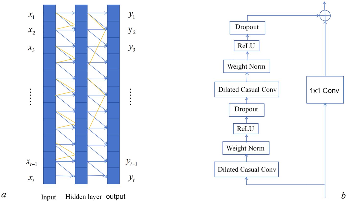
Figure 1. Architecture of the temporal convolutional network (TCN). (a) Dilated causal convolution. (b) Residual block.

2.3.2 Dilation convolution

Due to the existence of causal convolution, TCNs can only increase the network depth to obtain the timing information of sequences and obtain this feature from historical data. When applied to scenarios that require long-term historical information, in order to obtain sufficient temporal features, the traditional convolutional kernel must attempt to increase the depth of the network due to linear stacking, which makes it difficult for TCNs to face large-scale temporal tasks. The problem becomes simple when dilation convolution is applied, which introduces the concept of the expansion coefficient and allows the existence of interval samples in the convolutional inputs, thus allowing the sensing field of the convolution kernel to become exponentially expanded. As shown in Figure 1, the expansion coefficient of the first layer is 1; when the second layer is 3, the relationship between the receptive field and the number of hidden layers reaches an exponential level. The combination of causal and expansion convolution can greatly increase the receptive field of causal convolution, thus achieving historical information acquisition for long time series.

2.3.3 Residual link

Residual connection occurs when the input data can be directly connected to the subsequent layers for output across the previous intermediate layers. Neural networks have the problem of vanishing and exploding gradients, which is due to errors that keep stacking up and passing on as the network structure deepens, leading to the degradation of the neural network. To ensure that the outputs of the two branches have the same dimension, a one-dimensional convolution operation is used to control the data dimension. As shown in Figure 1, the left side is a two-layer causal expansion network, while the right side is the residual direct connection, which can be directly added to the convolution result. The mathematical expression is as Equation 10:

$\begin{array}{ll}{h}_{(x)}=x+f_{(x)}& (10)\end{array}$

where x is the residual connection input; ${\text{h}}_{(\text{x})}$ is the residual connection output; and $f_{(x)}$ is the nonlinear transformation.

2.4 Bidirectional gated recurrent unit model

The GRU is improved based on the LSTM neural network (Elmousaid et al., 2024), which has a simpler structure compared with the LSTM neural network that uses three gates. It has a reduced number of two gates, the updating and resetting gates, and is more effective. The formulas for the specific gate unit update are as Equations 11-14:

$\begin{array}{ll}{r}_t=\sigma (W_r·[h_{t-1},x_t]+b_r)& (11)\end{array}$

$\begin{array}{ll}{z}_t=\sigma (W_z·[h_{t-1},x_t]+{\text{b}}_{\text{z}})& (12)\end{array}$

$\begin{array}{ll}{\tilde{h}}_t=\varphi (W_{\hslash }·[r_t\times h_{t-1},x_t]+{\text{b}}_{\text{h}})& (13)\end{array}$

$\begin{array}{ll}{h}_t=(1-z_t)\times h_{t-1}+z_t\times {\tilde{h}}_t& (14)\end{array}$

where: $x_t,h_{t-1},h_t$ are the vectors of the input data; $\varphi$ is the hyperbolic tangent function; and $z_t$ and $r_t$ are the update gate and the reset gate, respectively. $\sigma$ is the sigmoid function. The update gate is used to control the percentage of information that is brought from the previous state to the next state. The reset gate controls how much information from the previous state is retained by the current candidate set. The principle is shown in Figure 2.

Figure 2

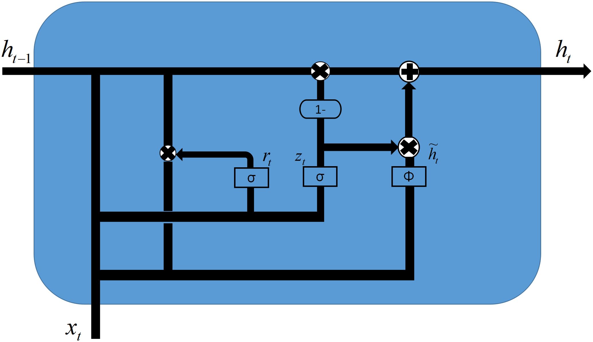
Figure 2. Flowchart of the gated recurrent unit (GRU).

A unidirectional GRU can only focus on the state before the prediction moment. However, the multidimensional ship traverse data have the bidirectionality of the time sequence; that is, the state in the forward and backward two time directions will have a certain impact on the prediction of the current moment. Therefore, a BiGRU network was adopted by connecting the unidirectional GRUs forward and backward, as shown in Figure 3. The BiGRU layer, which is able to analyze the states before and after two moments while expanding the field of view, is more in line with the actual characteristics of the multidimensional ship roll data.

Figure 3

Figure 3. Flowchart of the ship roll prediction model.

2.5 Self-attention mechanism

Self-attention is a type of attention mechanism that correlates different positions of a ship’s transverse motion sequence to compute a representation of the same time series. The self-attention mechanism is not concerned with the relationship between the data source and the output: it will only focus on the relationship between the different elements of the same sequence, even if these two elements are far away from each other. Therefore, the self-attention mechanism is very good at dealing with long-distance sequences and global information.

Its working principle, which is also known as the attention formula, is Equation 15:

$\begin{array}{ll}Attention(Q, K, V)=softmax\left(\frac{Q{K}^T}{\sqrt{d_k}}\right)& (15)\end{array}$

Here, the sources of the key values are all products of the input data matrices and are therefore all a linear transformation of the input data, which is where self-attention comes from.

2.6 Improved dung beetle optimization algorithm

The DBO algorithm is a new swarm intelligence optimization algorithm proposed by Xue and Shen (2023), which was developed from the behavior of dung beetles in nature and has been verified to have better performance than other swarm intelligence optimization algorithms. According to the behavioral characteristics of dung beetles, the algorithm was designed with five behavior patterns: dung beetle rolling, dancing, spawning, foraging, and stealing. In this case, both ball rolling and dancing behaviors can be classified as different behavioral patterns of the dung beetle ball rolling behavior in terms of whether or not it encounters an obstacle. According to the experience summarized from the simulation experiments for ship roll behavior prediction, the initial position and foraging stage is improved to make it more in line with the requirements of ship roll motion prediction.

Firstly, the mathematical model of the dung beetle individual position can be expressed as Equation 16:

$\begin{array}{ll}\begin{array}{l}{x}_i(t+1)=x_i(t)+\alpha k{x}_i(t-1)+b\Delta x\\ \Delta x=\left|x_i(t)-x_{\omega }\right|\end{array}& (16)\end{array}$

where t is the number of iterations; $x_i(t)$ is the position coordinate of the i-th dung beetle at the t-th iteration; k is the deflection coefficient; $b\in (0,1)$; α is either −1 or 1; $x_{\omega }$ is the global most unfavorable position; and Δx is the value of the change of intensity of the light source. The initial position of the dung beetle is randomly generated, but an undesirable random position may make the individual dung beetle fall into a local optimum. Furthermore, the addition of chaotic mapping will speed up its convergence and improve its performance. The use of cubic chaotic mapping can increase the particle diversity, which can reduce the particle optimization time and increase the convergence speed of the algorithm. The principle is shown in Equation 17:

$\begin{array}{ll}{x}_{n+1}=\rho x_n(1-x_n^2)& (17)\end{array}$

Secondly, the initial dung beetle foraging location update model is expressed as Equation 18:

$\begin{array}{ll}\begin{array}{l}{x}_i(t+1)=x_i(t)+C_1(x_i(t)-L_b)+\\ C_2(x_i(t)-U_b)\end{array}& (18)\end{array}$

where $x_i(t)$ denotes the position coordinates of the i-th adult dung beetle at the t-th iteration; C₁ and C₂ denote random numbers and random vectors belonging to (0,1) with normal distribution; and L_b and U_b are the upper and lower boundaries of the optimal foraging range, respectively. The food position must be reached before it can go to the next point. However, the triangular walking strategy does not need to be directly close to the food, but can walk around the food, increasing the randomness of the dung beetle. The formula for the triangle walk strategy is as Equation 19:

$\begin{array}{ll}\begin{array}{l}{L}_1=po{s}_b(t)-po{s}_c(t)\\ {\overrightarrow{L}}_2=rand()\times {\overrightarrow{L}}_1\end{array}& (19)\end{array}$

Afterward, the direction of travel $\beta$ is defined according to the Equation 20.

$\begin{array}{ll}\beta =2\times pi\times rang()& (20)\end{array}$

The Equation 21 is then used to obtain the position acquired after the little dung beetle has wandered away.

$\begin{array}{ll}\begin{array}{l}P=L_1^2+L_2^2-2\times L_1\times L_2\times \cos (\beta )\\ Po{s}_{new}=po{s}_b(t)+r+P\end{array}& (21)\end{array}$

This can improve the foraging speed of dung beetles, improve the convergence speed of the whole algorithm, and avoid falling into the local optimum.

2.7 Prediction model for ship roll motion (IDBO–TCN–BiGRU–Attention)

In this paper, we first combined TCN and BIGRU to construct a hybrid ship roll motion prediction model. As TCN has a strong ability to capture spatial information, and is dependent on the existence of causal convolution operation, it can also obtain historical information in long sequences. However, as it is after all a shallow neural network, TCN alone cannot fully obtain historical information. It can obtain the time series information in the data when combined with BiGRU. Nonetheless, when dealing with long sequences, self-attention has more advantages. Therefore, the self-attention mechanism is added and the IDBO algorithm is finally used to optimize the four hyper-parameters of the learning rate, the number of neurons in BiGRU, the key value of the attention mechanism, and the regularization parameters. Subsequently, the optimal value is assigned to the hybrid prediction model so that a better prediction effect can be obtained. The workflow is shown in Figure 3.

3 Simulation experiments and analysis of results

3.1 Experimental data

The experimental data were based on the measured data of the training ship “Yukun” of Dalian Maritime University. “Yukun” was carrying out the “L” maneuver in the northeast sea area of Weihai when the data were collected. The ship motion attitude data were collected using the “ADU2” data acquisition instrument installed on the bow and stern and the side of the ship, with a collection frequency of 1 Hz. Data collection was from 10:48:00 on August 12, 2012, to 11:06:20 on August 12, 2012, with a total of 1,100 sets of data. For the purpose of training and testing the proposed prediction model, the data were partitioned into two subsets: the first 80% of the data, corresponding to 880 data points, was designated as the training set, while the remaining 20%, or 220 data points, was reserved as the test set. This division ensures that the model is both rigorously trained on a substantial amount of data and evaluated on an independent set to assess its generalization capability.

3.2 Performance evaluation indicators

The root mean square error (RMSE), mean absolute error (MAE), mean square error (MSE), mean absolute percentage error (MAPE), and coefficient of determination are commonly used in a regression task. The smaller the value, the higher the prediction accuracy of the model, and the higher the coefficient of determination, the higher the model credibility. Therefore, we utilized the RMSE, MAE, MSE, and MAPE to evaluate the performance of the prediction model. Equation 22 is the related formulas:

$\begin{array}{ll}\begin{array}{l}MAE=\frac{1}{n}{\displaystyle {\sum }_{i=1}^n\left|y_i-{\tilde{y}}_i\right|}\hfill \\ MSE=\frac{1}{n}{\displaystyle {\sum }_{i=1}^n{\left|y_i-{\tilde{y}}_i\right|}^2}\hfill \\ RMSE=\sqrt{\frac{1}{n}{\displaystyle {\sum }_{i=1}^n{\left|y_i-{\tilde{y}}_i\right|}^2}}\hfill \\ MAPE=\frac{1}{n}{\displaystyle {\sum }_{i=1}^n\frac{\left|y_i-{\tilde{y}}_i\right|}{y_i}}\hfill \end{array}& (22)\end{array}$

where $y_i$ denotes the true value at moment t; ${\tilde{y}}_i$ denotes the predicted value at moment t; and n denotes the number of true values.

$\begin{array}{ll}{R}^2=1-\frac{{\sum }_i{(\widehat{y_i}-y_i)}^2}{{\sum }_i{(\overline{y_i}-y_i)}^2}& (23)\end{array}$

Equation 23 is the formula for the coefficient of determination, where the numerator part represents the sum of the squared differences between the true and the predicted values, similar to the mean square deviation, while the denominator part represents the sum of the squared differences between the true and the mean values, similar to the variance.

3.3 Fitness function of VMD

According to the collected experimental data of the “Yukun,” we used four fitness functions to decompose the roll motion data of the ship. The results are shown in Figure 4. When the minimum envelope entropy (Figure 4A), the minimum permutation entropy (Figure 4B), and the minimum sample entropy (Figure 4D) were used as the fitness functions, the ship roll motion data were decomposed into more than seven modal functions. Even Figures 4B, D were decomposed into more than nine modes. Only the minimum information entropy (Figure 4B) was used as the fitness function for decomposition into six eigenmodal functions. The residuals of the reconstructed data were obtained when the decomposed data were reconstructed, and the difference between the original data in Figure 5 can be clearly seen to be not much different. However, the effect in Figure 5D looks better. From the data in Table 1, it can be seen that the residuals of the decomposition of the four fitness functions are not much different. The difference in the minimum sample entropy was the smallest, but the time taken was more than five times that of the minimum information entropy. Moreover, the residuals and the time of the minimum information entropy were less than those of the minimum envelope entropy. Hence, it is more suitable to choose the minimum information entropy after verification.

Figure 4

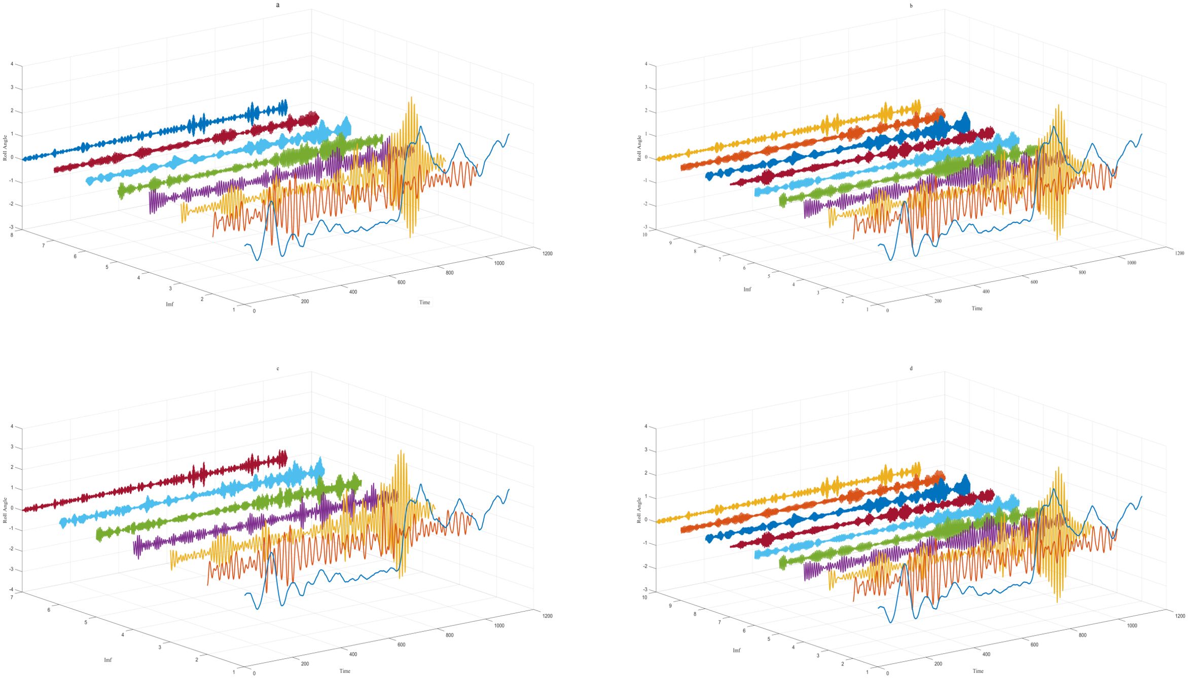
Figure 4. (a–d) Decomposition results on the roll status data.

Figure 5

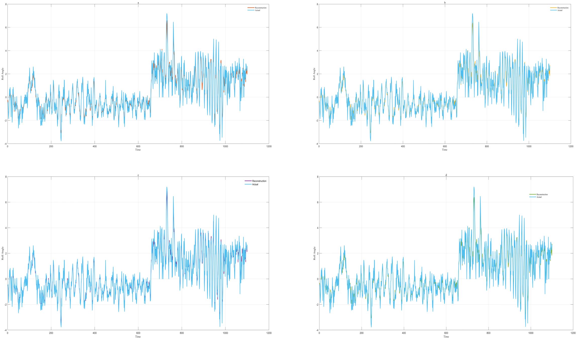
Figure 5. (a–d) Reconstruction error based on different fitness functions.

Table 1

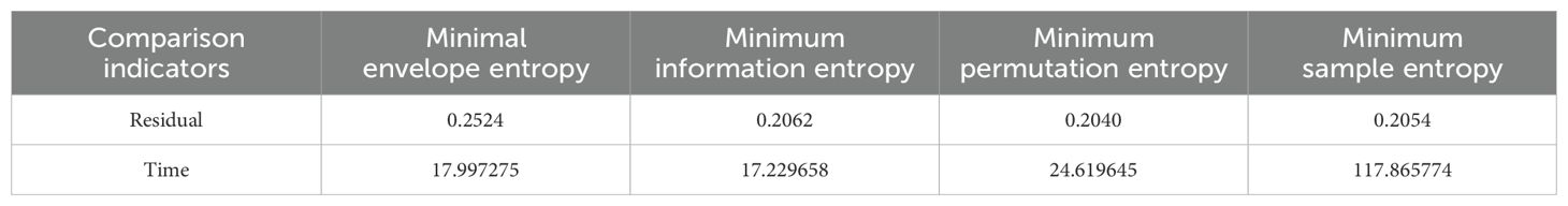
Table 1. Residuals and decomposition time for the four fitness functions.

3.4 Comparison of the forecast results of the different algorithms

The roll motion data of the ship were a time series with complex, nonlinear, and non-stationary characteristics. There are many algorithms for time series prediction. Which algorithm to use is also the first problem in the study of the prediction of the roll motion of ships. In order to use appropriate algorithms for research on ship roll forecasting, this paper used a number of commonly used algorithms, namely, back-propagation (BP), SVM, relevance vector machine (RVM), CNN, LSTM, GRU, TCN, and BiGRU, to conduct simulation and comparison experiments using the measured ship roll motion data. Based on the results of the comparisons, it was determined which method is more appropriate.

As shown in Figure 6, the prediction results of these eight algorithms were compared with the actual data. It can be seen that these algorithms can correctly predict the trend of ship roll motion; however, BP and CNN both had large fluctuations around the end of the 210-s prediction. The prediction results of GRU, RVM, and LSTM tended to be flat, and there was a large error with the actual value. The prediction effect of SVM was quite good, but its determination coefficient was low. The prediction results of TCN and BiGRU had certain advantages compared with the other six algorithms. As shown in Figure 7, except for the obvious large deviation of CNN, the rest of the differences were small. Of course, it can be observed that each prediction effect was not very ideal, which may be related to the fact that unprocessed multidimensional data input was used. However, the residuals of the other seven algorithms were very stable, and there were no large fluctuations, as can be seen from Table 2. The evaluation indicators of the TCN and BiGRU algorithms were in the forefront, particularly the coefficient of determination being close to 60%. It can be seen from Figure 8 that, in addition to the coefficient of determination, the other four evaluation indicators showed a downward trend in the TCN and BiGRU algorithms. This indicates that these two models are more suitable for the prediction of ship roll motion.

Figure 6

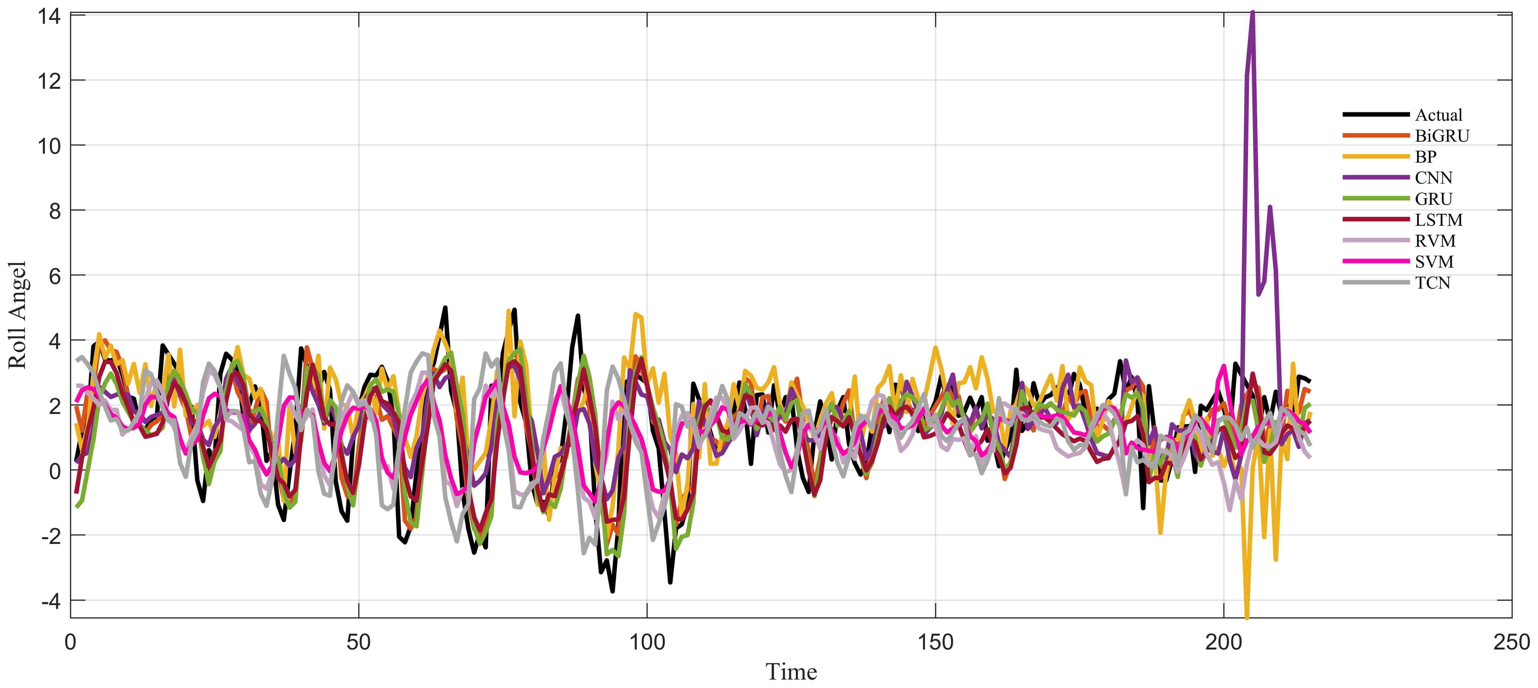
Figure 6. Comparison of the prediction results of the different algorithms with actual data.

Figure 7

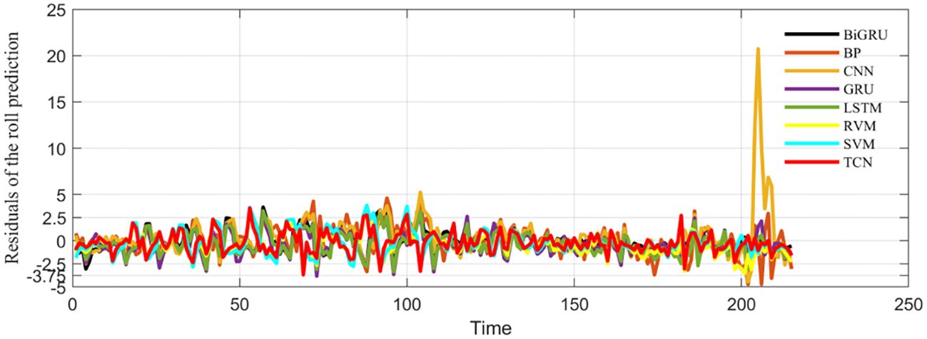
Figure 7. Comparison of the prediction errors of the different algorithms with actual data.

Table 2

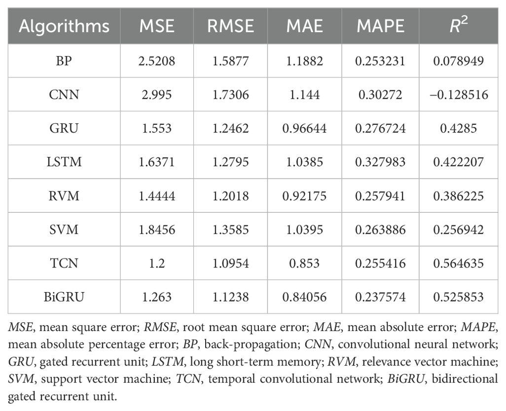
Table 2. Comparison of the evaluation metrics for the different algorithms.

Figure 8

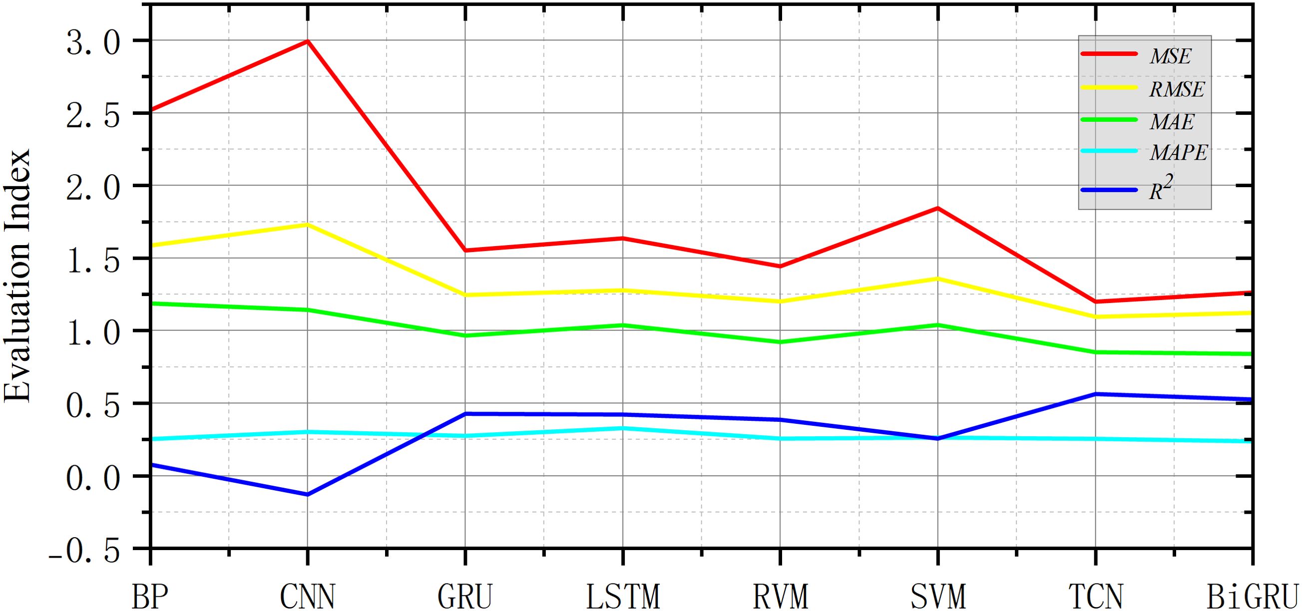
Figure 8. Numerical curves of the different algorithms for mean square error (MSE), root mean square error (RMSE), mean absolute error (MAE), mean absolute percentage error (MAPE), and R2.

3.5 Comparison of the prediction results of the combined model

Based on the results of the comparative experiments on the algorithms, TCN and BiGRU were found to be more suitable for ship roll prediction. Therefore, based on these two algorithms, a hybrid ship roll motion prediction model was built, this time using the VMD algorithm to decompose the input roll data. The PCA was then used to reduce the dimensionality. The original data were reconstituted into the input data, and the input data were compared with VMD–PCA–TCN and VMD–PCA–BiGRU.

Firstly, after Pearson’s correlation analysis, it can be seen from Figure 9 that the correlation coefficient between the ship’s longitude and latitude displacement, ground course, and ground speed and the ship’s roll motion was greater than 0.5, and its correlation was large. After the comparative experiments, it can be seen from Figure 10 that the prediction results of VMD–PCA–BiGRU were very close to the measured data, with the data from VMD–PCA–TCN being second only to the former. However, there was a large error. The results of TCN and BiGRU were still relatively stable, basically consistent with the trend of the measured data, and the error was not very large. It can be seen from Figure 11 that the error of VMD–PCA–TCN was the smallest and has been very stable, while those of the other two had large fluctuations. In particular, the TCN error was the largest compared with those of the other three. According to Figure 12 and Table 3, it is noticeable that the evaluation indicators of VMD–PCA–TCN and VMD–PCA–BiGRU nearly doubled compared with those of TCN and BiGRU, except for the MAPE, which showed a relatively flat decline.

Figure 9

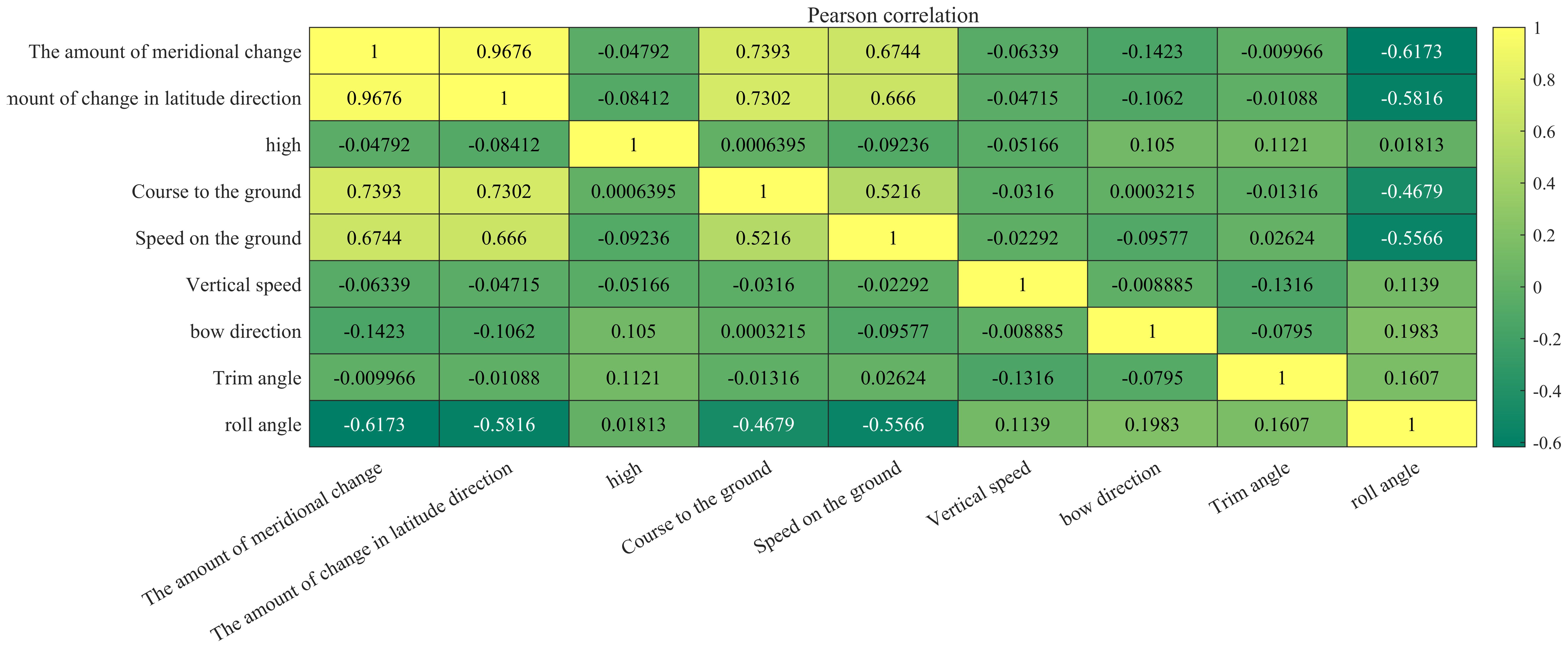
Figure 9. Pearson’s correlations.

Figure 10

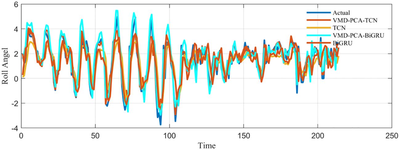
Figure 10. Comparison of the prediction results of the combined models with the actual data.

Figure 11

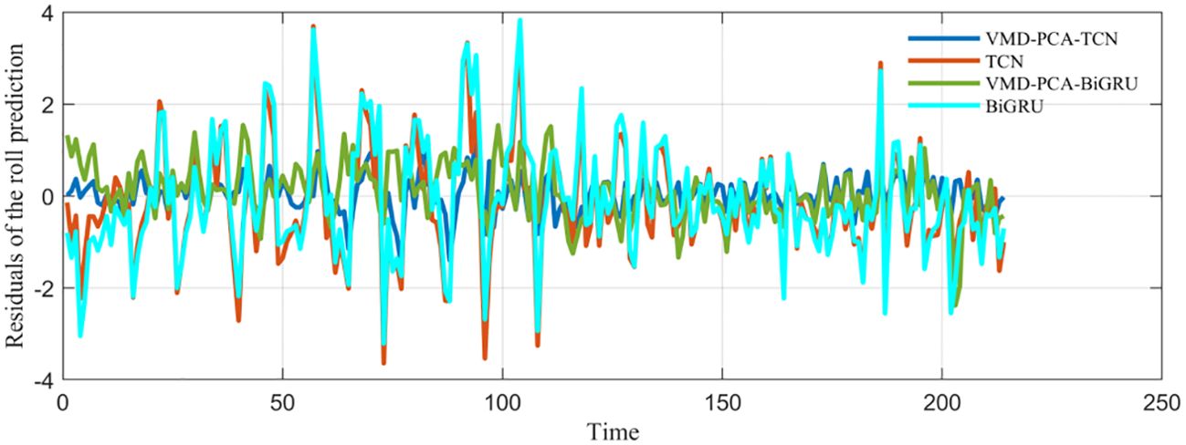
Figure 11. Comparison of the prediction errors of the combined models with the actual data.

Figure 12

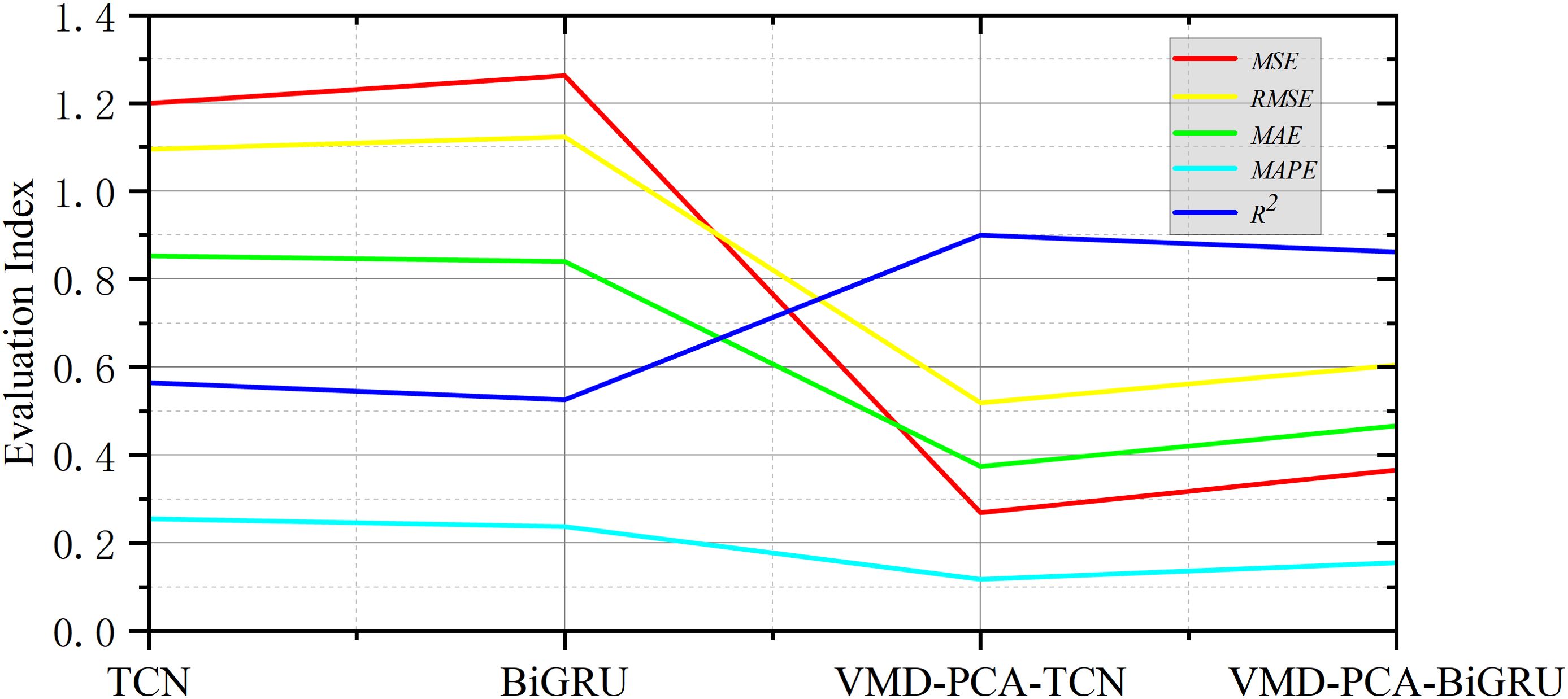
Figure 12. Numerical curves of the combined models for mean square error (MSE), root mean square error (RMSE), mean absolute error (MAE), mean absolute percentage error (MAPE), and R2.

Table 3

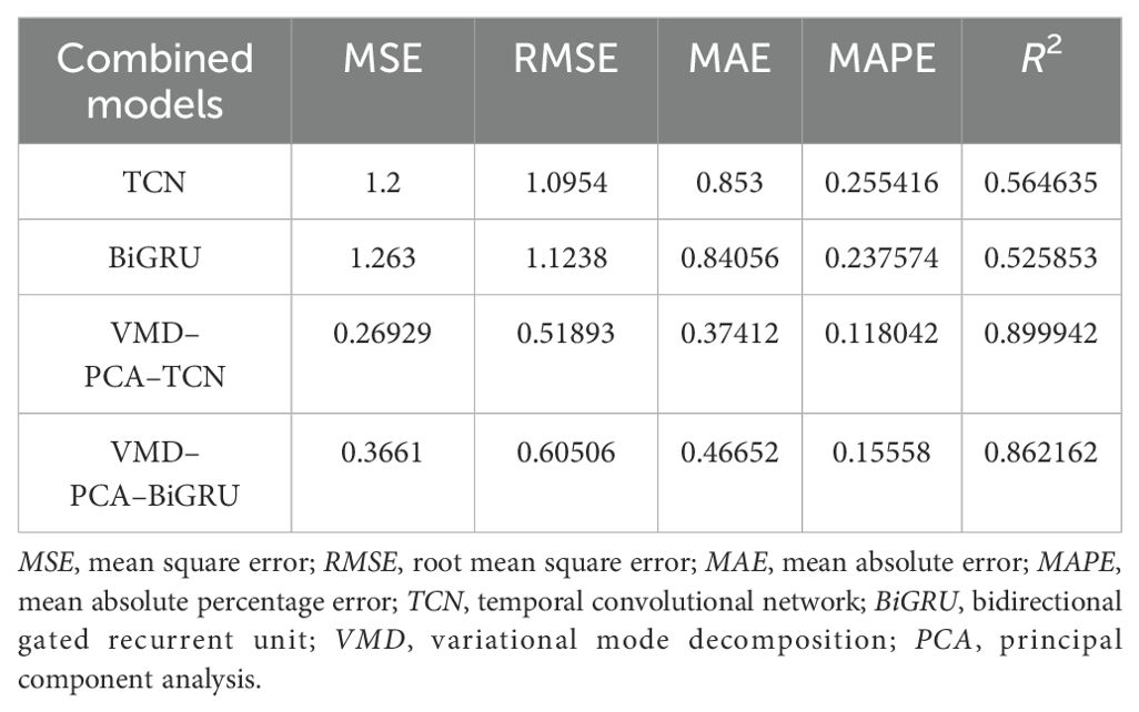
Table 3. Comparison of the evaluation metrics for the combined models.

3.6 Ablation experiments

Ablation experiments were carried out. Each time the removal of a module in the hybrid ship roll prediction model is experimented, each round of experiments is carried out for 10 rounds. The average value was taken to exclude the influence of accidental factors, as observed in Figure 13. It can be seen from the comparison between TCN–BiGRU and VMD–PCA–TCN–BiGRU obtained after adding the data processing module that the four evaluation indicators declined rapidly, while only the MAPE decreased slowly. The comparison between VMD–PCA–TCN–BiGRU and VMD–PCA–TCN–BiGRU–Attention with the self-attention mechanism showed that the MSE and RMSE in the evaluation index had a significant decrease, while the rest of the values were not obvious. This trend was very noticeable after the addition of the optimization algorithm, while the downward trend was not too obvious after the addition of the IDBO algorithm. It can be seen from Table 4 that the four evaluation indicators, i.e., MSE, RMSE, MAE, and MAPE, decreased. The coefficient of determination was also increased, as shown in Figure 14. The prediction results of VMD–PCA–TCN–BiGRU–Attention, VMD–PCA–DBO–TCN–BiGRU–Attention, and VMD–PCA–IDBO–TCN–BiGRU–Attention were the closest to the measured data, which was very noticeable around 80 s. Figure 15 shows that the VMD–PCA–TCN–BiGRU–Attention model was consistent and stable, fluctuating greatly around 190 s, but quickly regaining stability. The rest of the combinations remained in a stable error range.

Figure 13

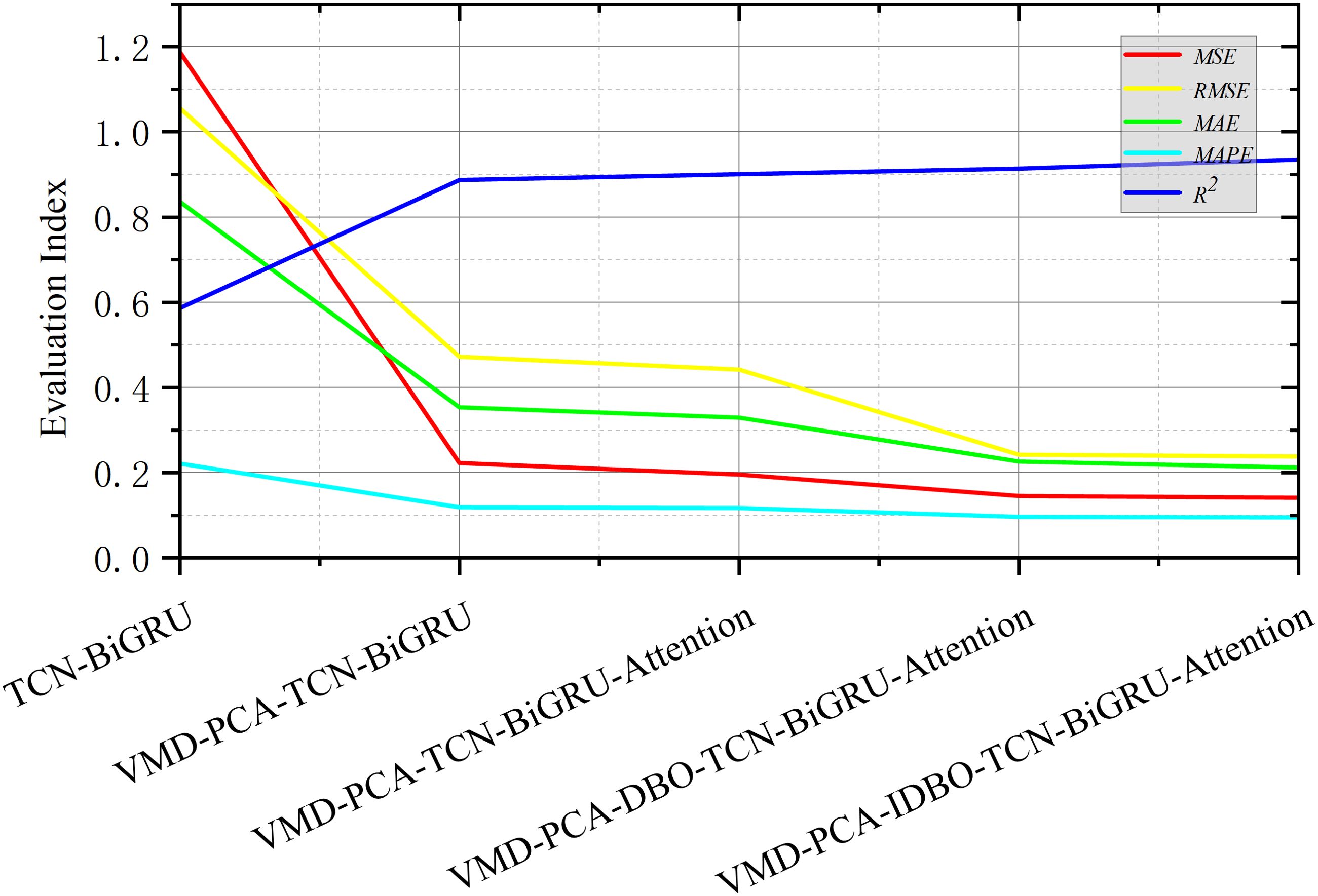
Figure 13. Numerical curves on the ablation experimental models for mean square error (MSE), root mean square error (RMSE), mean absolute error (MAE), mean absolute percentage error (MAPE), and R2.

Table 4

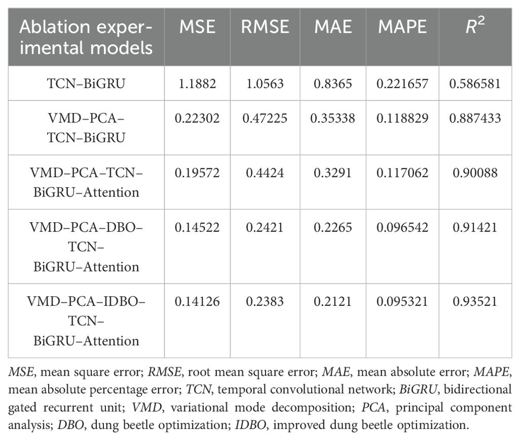
Table 4. Comparison of the evaluation metrics for the ablation experimental models.

Figure 14

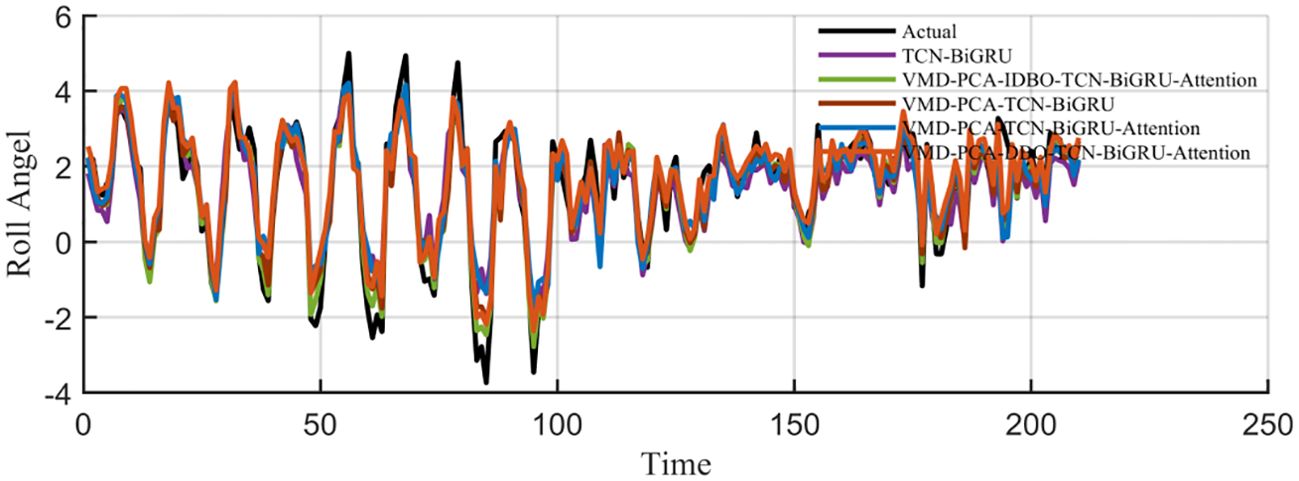
Figure 14. Comparison of the prediction results of the ablation experimental models with the actual data.

Figure 15

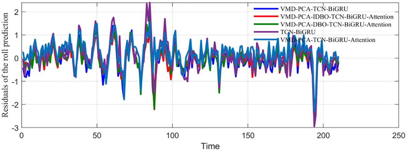
Figure 15. Comparison of the prediction errors of the ablation experimental models with the actual data.

4 Conclusion and discussion

Due to the complex maritime environment and the powerful rocking motion of ships, it is necessary to carry out an accurate prediction of a ship’s roll motion in order to improve the safety of ship navigation, the comfort of the ship’s personnel, and the efficiency of offshore management. Therefore, this paper proposed a hybrid ship roll motion prediction model based on the decomposition algorithm and the deep learning model. The roll motion data of the ship were decomposed and reduced using the VMD–PCA algorithm to reconstruct the new input data. Subsequently, the TCN–BiGRU–Attention model was input for forecasting, and the IDBO algorithm was used to optimize the hyper-parameters. The results showed that: 1) the VMD–PCA–IDBO–TCN–BiGRU–Attention hybrid prediction model proposed in this paper had high prediction accuracy and good prediction effect; 2) the data processing method of the VMD–PCA proposed in this paper had a significant effect on the data of the unstable time-varying characteristics of the ship roll motion and improved the accuracy of prediction models such as the TCN, BiGRU, and TCN–BiGRU; 3) the effect of improving the DBO algorithm was noticeable, which can improve the prediction effect of the high-precision model; and 4) the effect of the self-attention mechanism was not very noticeable when dealing with short sequences, with the self-attention effect being better when dealing with large databases. Overall, the ship motion prediction model showcased outstanding performance on complex datasets, effectively capturing the temporal dynamics and nonlinear behaviors of ship motion. It was proven to be superior in terms of prediction accuracy, convergence speed, and adaptability, offering valuable insights into the future of ship navigation and safety management. By providing a reliable support tool for maritime operations, this model holds significant promise for enhancing the safety and efficiency of ship navigation.

However, several limitations remain, which warrant further investigation. The current model focuses solely on the ship’s intrinsic motion state, without considering external environmental factors such as wind, waves, and currents, which also play a crucial role in a ship’s movement. In addition, the model’s current implementation is based on short-term, off-line predictions, which may not be sufficient for real-time, online forecasting in dynamic maritime environments. This raises the need for further research into the feasibility of deploying the model in an online, real-time setting. Moreover, exploring the potential for lightweight deployment on embedded devices could enhance the practical applications and efficiency of the model, particularly in real-world maritime operations, where real-time prediction is critical. These future directions could expand the utility and scalability of the model, paving the way for broader use in maritime safety and management systems.

Data availability statement

The original contributions presented in the study are included in the article/supplementary material. Further inquiries can be directed to the corresponding author.

Author contributions

HW: Writing – original draft, Writing – review & editing. JY: Conceptualization, Data curation, Investigation, Methodology, Software, Supervision, Writing – original draft. NW: Formal Analysis, Project administration, Validation, Writing – review & editing. LW: Funding acquisition, Resources, Visualization, Writing – review & editing.

Funding

The author(s) declare that financial support was received for the research and/or publication of this article. This work was supported by the National Natural Science Foundation of China under grants 52231014 and 52271361, the Special Projects of Key Areas for Colleges and Universities in Guangdong Province under Grant 2021ZDZX1008, the Natural Science Foundation of Guangdong Province of China under Grant 2023A1515010684, the Technology breakthrough plan project of Zhanjiang under Grant 2023B01024, and the Program for Scientific Research Start-Up Funds of Guangdong Ocean University.

Conflict of interest

The authors declare that the research was conducted in the absence of any commercial or financial relationships that could be construed as a potential conflict of interest.

Generative AI statement

The author(s) declare that no Generative AI was used in the creation of this manuscript.

Publisher’s note

All claims expressed in this article are solely those of the authors and do not necessarily represent those of their affiliated organizations, or those of the publisher, the editors and the reviewers. Any product that may be evaluated in this article, or claim that may be made by its manufacturer, is not guaranteed or endorsed by the publisher.

References

Agga A., Abbou A., Labbadi M., Houm Y. E., and Ou Ali I. H. (2022). CNN-LSTM: An efficient hybrid deep learning architecture for predicting short-term photovoltaic power production. Electric Power Syst. Res. 208, 107908. doi: 10.1016/j.epsr.2022.107908

Crossref Full Text | Google Scholar

Bai S., Kolter J. Z., and Koltun V. (2018). An empirical evaluation of generic convolutional and recurrent networks for sequence modeling. arXiv preprint. doi: 10.48550/arXiv.1803.01271

Crossref Full Text | Google Scholar

Bhunia A. K., Konwer A., Bhunia A. K., Bhowmick A., Roy P. P., Pal U., et al. (2019). Script identification in natural scene image and video frames using an attention based Convolutional-LSTM network. Pattern Recogn. 85, 172–184. doi: 10.1016/j.patcog.2018.07.034

Crossref Full Text | Google Scholar

Bo Z. and Shi A. (2013). Empirical Mode Decomposition Based LSSVM for Ship Motion Prediction Vol. 2013 (Berlin, Heidelberg: Springer), 319–325.

Google Scholar

Broome D. R. and Hall M. S. (1998). Application of ship motion prediction. Int. Marit. Technol. 10, 77–93. Available online at: http://pascal-francis.inist.fr/vibad/index.php?action=getRecordDetail&idt=1587453.

Google Scholar

Cheng X., Li G., Skulstad R., Major P., Chen S., Hildre H. P., et al. (2019). Data driven uncertainty and sensitivity analysis for ship motion modeling in offshore operations. Ocean Eng. 179, 261–272. doi: 10.1016/j.oceaneng.2019.03.014

Crossref Full Text | Google Scholar

Cui X., Zhu J., Jia L., Wang J., and Wu Y. (2024). A novel heat load prediction model of district heating system based on hybrid whale optimization algorithm (WOA) and CNN-LSTM with attention mechanism. Energy 312, 133536. doi: 10.1016/j.energy.2024.133536

Crossref Full Text | Google Scholar

Dragomiretskiy K. and Zosso D. (2014). Variational mode decomposition. IEEE Trans. Signal Process. 62, 531–544. doi: 10.1109/TSP.2013.2288675

Crossref Full Text | Google Scholar

Eckert-Gallup A. C., Sallaberry C. J., Dallman A. R., and Neary V. S. (2016). Application of principal component analysis (PCA) and improved joint probability distributions to the inverse first-order reliability method (I-FORM) for predicting extreme sea states. Ocean Eng. 112, 307–319. doi: 10.1016/j.oceaneng.2015.12.018

Crossref Full Text | Google Scholar

Elmousaid R., Drioui N., Elgouri R., Agueny H., and Adnani Y. (2024). Ultra-short-term global horizontal irradiance forecasting based on a novel and hybrid GRU-TCN model. Results Eng. 23, 102817. doi: 10.1016/j.rineng.2024.102817

Crossref Full Text | Google Scholar

Fossen T. (2011). Handbook of Marine Craft Hydrodynamics and Motion Control (New York, USA and Beijing, China: John Wiley & Sons and science press).

Google Scholar

Fu J., Wu C., Wang J., Haque M. M., Geng L., and Meng J. (2024). Lithium-ion battery SOH prediction based on VMD-PE and improved DBO optimized temporal convolutional network model. J. Energy Storage 87, 111392. doi: 10.1016/j.est.2024.111392

Crossref Full Text | Google Scholar

Gao N., Hu A., Hou L., and Chang X. (2023). Real-time ship motion prediction based on adaptive wavelet transform and dynamic neural network. Ocean Eng 280, 114466. doi: 10.1016/j.oceaneng.2023.114466

Crossref Full Text | Google Scholar

Geng X., Sun Q., Li Y., Zhang S., Zhou Z., and Wang Y. (2024). A data-driven data-augmentation method based on slim-generative adversarial imputation networks for short-term ship-motion attitude prediction. Ocean Eng. 299, 117364. doi: 10.1016/j.oceaneng.2024.117364

Crossref Full Text | Google Scholar

Guan B. L., Yang W., Wang Z. B., and Tang Y. G. (2018). Ship roll motion prediction based on ℓ1 regularized extreme learning machine. PloS One 13, e0206476. doi: 10.1371/journal.pone.0206476

PubMed Abstract | Crossref Full Text | Google Scholar

Huang L. M., Duan W. Y., Yang H., and Chen Y. S. (2014). A review of short-term prediction techniques for ship motions in seaway. J. Ship Mech. 18, 1534–1542. doi: 10.3969/j.issn.1007-7294.2014.12.013

Crossref Full Text | Google Scholar

Jiang H., Duan S. L., Huang L. M., Han Y., Yang H., and Ma Q. W. (2020). Scale effects in AR model real-time ship motion prediction. Ocean Eng. 203, 107202. doi: 10.1016/j.oceaneng.2020.107202

Crossref Full Text | Google Scholar

Kaplan P. (1969). A study of prediction techniques for aircraft carrier motions at sea. Hydronaut 3, 121–131. doi: 10.2514/3.62814

Crossref Full Text | Google Scholar

Li G., Zhang H., Lyu T., and Zhang H. (2024). Regional significant wave height forecast in the east China sea based on the self-attention ConvLSTM with SWAN model. Ocean Eng. 312, 119064. doi: 10.1016/j.oceaneng.2024.119064

Crossref Full Text | Google Scholar

Li M. W., Geng J., Han D.-F., and Zheng T. J. (2016). Ship motion prediction using dynamic seasonal RvSVR with phase space reconstruction and the chaos adaptive efficient FOA. Neurocomputing 174, 661–680. doi: 10.1016/j.neucom.2015.09.089

Crossref Full Text | Google Scholar

Liu Y., Ning C., Zhang Q., Yuan G., and Li C. (2024). Utilizing VMD and BiGRU to predict the short-term motion of buoys. Ocean Eng. 313, 119237. doi: 10.1016/j.oceaneng.2024.119237

Crossref Full Text | Google Scholar

Moon J., Hossain M. B., and Chon K. H. (2021). AR and ARMA model order selection for time series modeling with ImageNet classification. Signal Process. 183, 108026. doi: 10.1016/j.sigpro.2021.108026

Crossref Full Text | Google Scholar

Ni C. H. and Ma X. D. (2020). An integrated long-short term memory algorithm for predicting polar westerlies wave height. Ocean Eng. 215, 107715. doi: 10.1016/j.oceaneng.2020.107715

Crossref Full Text | Google Scholar

Peng X. Y. (2023). Adaptive Modeling and Prediction of Ship Motion (Science Press).

Google Scholar

Sadrara M. and Khorrami M. K. (2023). Principal component analysis–multivariate adaptive regression splines (PCA-MARS) and back propagation-artificial neural network (BP-ANN) methods for predicting the efficiency of oxidative desulfurization systems using ATR-FTIR spectroscopy. Spectrochimica Acta Part A: Mol. Biomolecular Spectrosc. 300, 122944. doi: 10.1016/j.saa.2023.122944

PubMed Abstract | Crossref Full Text | Google Scholar

Su Y. M., Lin J. F., Zhao D. G., Guo C. Y., Wang C., and Guo H. (2020). Real-time prediction of large-scale ship model vertical acceleration based on recurrent neural network. Marine Sci. Eng. 8, 777. doi: 10.3390/jmse8100777

Crossref Full Text | Google Scholar

Takami T., Nielsen U. D., and Jensen J. J. (2021). Real-time deterministic prediction of wave induced ship responses based on short-time measurements. Ocean Eng. 221, 108503. doi: 10.1016/j.oceaneng.2020.108503

Crossref Full Text | Google Scholar

Triantafyllou M. S. and Athans M. (1981). Real Time Estimation of the Heaving and Pitching Motions of a Ship Using a Kalman Filter (Boston MA: IEEE).

Google Scholar

Wang L. L., Li X., and Bai Y. L. (2018). Short-term wind speed prediction using an extreme learning machine model with error correction. Energy Convers. Manage. 162, 239–250. doi: 10.1016/j.enconman.2018.02.015

Crossref Full Text | Google Scholar

Wang P. L., Zhang T., and Xiao Y. J. (2021). Prediction of ship pitch angle based on improved PSO-ARIMA model. J. Shanghai Marit. Univ. 42, 39–43. doi: 10.13340/j.jsmu.2021.01.007

Crossref Full Text | Google Scholar

Xu D. and Yin J. (2024). An enhanced hybrid scheme for ship roll prediction using support vector regression and TVF-EMD. Ocean Eng. 307, 117951. doi: 10.1016/j.oceaneng.2024.117951

Crossref Full Text | Google Scholar

Xue J. and Shen B. (2023). Dung beetle optimizer: A new meta-heuristic algorithm for global optimization. J. Supercomput 79, 7305–7336. doi: 10.1007/s11227-022-04959-6

Crossref Full Text | Google Scholar

Yin J. C., Perakis A. N., and Wang N. (2018). A real-time ship roll motion prediction using wavelet transform and variable RBF network. Ocean Eng. 160, 10–19. doi: 10.1016/j.oceaneng.2018.04.058

Crossref Full Text | Google Scholar

Zafeiraki M. (2022). A comparison of ARIMA and SVR in short-term ship motion prediction. (Utrecht, Netherlands: Utrecht Univ).

Google Scholar

Zhang B., Wang S., Deng L., Jia M., and Xu J. (2023). Ship motion attitude prediction model based on IWOA-TCN-Attention. Ocean Eng. 272, 113911. doi: 10.1016/j.oceaneng.2023.113911

Crossref Full Text | Google Scholar

Zhang D., Zhou X., Wang Z.-H., Peng Y., and Xie S.-R. (2023). A data driven method for multi-step prediction of ship roll motion in high sea states. Ocean Eng. 276, 114230. doi: 10.1016/j.oceaneng.2023.114230

Crossref Full Text | Google Scholar

Zhang L., Feng X., Wang L., Gong B., and Ai J. (2024). A hybrid ship-motion prediction model based on CNN–MRNN and IADPSO. Ocean Eng. 299, 117428. doi: 10.1016/j.oceaneng.2024.117428

Crossref Full Text | Google Scholar

Zhang T., Zheng X. Q., and Liu M. X. (2021). Multiscale attention-based LSTM for ship motion prediction. Ocean Eng. 230, 109066. doi: 10.1016/j.oceaneng.2021.109066

Crossref Full Text | Google Scholar

Zhang Z. D., Ye L., Qin H., Liu Y. Q., Wang C., Yu X., et al. (2019). Wind speed prediction method using shared weight long short-term memory network and Gaussian process regression. Appl. Energy 247, 270–284. doi: 10.1016/j.apenergy.2019.04.047

Crossref Full Text | Google Scholar

Zhou T., Yang X., Ren H., Li C., and Han J. (2023). The prediction of ship motion attitude in seaway based on BSO-VMD-GRU combination model. Ocean Eng. 288, 115977. doi: 10.1016/j.oceaneng.2023.115977

Crossref Full Text | Google Scholar