Physics-informed neural networks to reconstruct surface velocity field from drifter data

Bang, Chiron; Altaher, Ali Salem; Zhuang, Hanqi; Altaher, Ahmed; Srinivasan, Ashwanth; Chérubin, Laurent M.

doi:10.3389/fmars.2025.1547995

ORIGINAL RESEARCH article

Front. Mar. Sci., 10 September 2025

Sec. Physical Oceanography

Volume 12 - 2025 | https://doi.org/10.3389/fmars.2025.1547995

Physics-informed neural networks to reconstruct surface velocity field from drifter data

Chiron Bang¹

Ali Salem Altaher^1,2

Hanqi Zhuang¹

Ahmed Altaher^1,3

Ashwanth Srinivasan⁴

Laurent M. Chérubin^5*

¹Department of Electrical Engineering and Computer Science, Florida Atlantic University, Boca Raton, FL, United States
²College of Medicine, Ibn Sina University of Medical and Pharmaceutical Science, Baghdad, Iraq
³Electronic Computer Center, Al-Nahrain University, Baghdad, Iraq
⁴Tendral, LLC, Miami, FL, United States
⁵Harbor Branch Oceanographic Institute, Florida Atlantic University, Fort Pierce, FL, United States

Accessing ocean velocity data is critical to improving our understanding of ocean dynamics, which affects our prediction capabilities for a range of services that the ocean provides. Because ocean current velocity information is scarce, prediction efforts have mostly relied on numerical models of ocean physics to reconstruct and predict velocity fields at desired spatial and temporal resolutions. However, numerical models, by design, are a simplified representation of the physics laws that govern ocean dynamics, hence error-prone even with data assimilation. Although accurate measurements of the flow field can be obtained using ocean drifters along their trajectories, their Lagrangian nature and sparsity make them unfit to provide direct Eulerian measurements. To address this issue, we apply a deep learning model called Physics-Informed Neural Networks (PINN) to reconstruct ocean surface velocity fields using sparse measurements obtained from drifters. We show that the physics learning part of the network is essential for the accurate reconstruction of the velocity field. In particular, we show the poor performance of the same deep neural network without the physics part, which reveals the ability of the partial differential equations derived by the PINN to capture the flow features’ dynamics. Our method is evaluated on both virtual and real drifters datasets. The reconstructed flow fields reveal the role of small-scale features in improving the representation of mesoscale flow dynamics.

1 Introduction

Satellite-tracked drifters (Sybrandy, 1991) provide direct measurements of currents throughout much of the world’s oceans, offering a unique tool to examine processes such as mean and eddy transport of momentum and heat. In response to the Deepwater Horizon oil spill in the Gulf of Mexico (GoM), a significant amount of research was conducted aimed at better predicting oil dispersion. Tools to better understand the dispersal properties of GoM waters included the design of new drifters (Novelli et al., 2017) and drifter release experiments. For example, the Lagrangian Submesoscale Experiment (LASER) between January and April 2016; the Submesoscale Processes and Lagrangian Analysis on the Shelf (SPLASH) between April and June 2017 among others as described in Lilly and Pérez-Brunius (2021). The latter used a large set of historical surface drifter data from the GoM – 3770 trajectories spanning 28 years and more than a dozen data sources - to create a gridded surface current product called GulfFlow.

While drifters have the unique ability to resolve sea surface velocity at multiple temporal and spatial scales, they present a significant drawback: the sparsity of the data collected. Drifters cannot cover a large area and, most importantly, they only provide information on their trajectories. On the other hand, having access to measurements over an entire region such as the GoM at a chosen time and spatial resolution is crucial for a better understanding of the dynamics of the ocean. Drifters are often treated as moving current meters. Most drifter data are used to understand the transport properties of the flow (Lumpkin and Johnson, 2013) and the Lagrangian characteristics (Mariano et al., 2016; Miron et al., 2017; Deyle et al., 2024). Velocity field estimation from drifter data is mostly used to obtain near-surface velocity climatology for the global ocean (Lumpkin, 2003).

Assimilating drifter velocities or Lagrangian trajectories in numerical models to improve their predictive capacity requires the estimation of the Eulerian velocity field. Two main approaches have been proposed for the assimilation of Lagrangian data. The first approach is based on estimating velocities along trajectories as the ratio between observed position differences and time increments (e.g.,Hernandez et al. (1995)) and directly using these velocities to correct the model results. The second approach introduces an observational operator based on the particle advection equation and corrects the Eulerian velocity field by requiring the minimization of the difference between observed and modeled trajectories (e.g. Molcard et al. (2003)).

Other efforts include methods based on augmenting the state vector of the prognostic variables with the Lagrangian drifter coordinates at assimilation and compute the evolution of the error covariance matrix with the extended Kalman filter (Ide et al., 2002; Kuznetsov et al., 2003; Salman et al., 2006). Lagrangian variational analysis methods allow for statistically robust reconstructions of velocity fields either directly from purely Lagrangian observations or from combinations of Eulerian model/data and Lagrangian datasets. The variational method of (Taillandier et al., 2006a) has been applied to the assimilation of Argo float data in the northwestern Mediterranean Sea (Taillandier et al., 2006b, 2010) and to the reconstruction of the velocity field in the Adriatic Sea (Taillandier et al., 2008). In the latter study, the velocity field reconstruction is only validated through the predicted trajectories of virtual drifters that are compared to the circulation features in Moderate Resolution Imaging Spectroradiometer (MODIS) chlorophyll-a images.

In recent years, machine learning methods have become popular in the field of remote sensing data recovery (Sonnewald et al., 2021; Hu et al., 2021; Park et al., 2019). Previous works have attempted to reconstruct the surface velocity field by using various types of data such as velocity, temperature, salinity, and sea surface height (SSH) (Martin et al., 2023; Thiria et al., 2023). For example, the relationship between salinity and temperature can be used to reconstruct the surface velocity field using convolutional neural networks (Isern-Fontanet et al., 2020). Sinha and Abernathey (2021) leveraged multiple global variables, specifically SSH, sea surface temperature (SST), sea surface salinity (SSS), and wind stress, as input to an artificial neural network to predict surface velocity. Using a local stencil of neighboring grid points as additional input features, they train their deep learning models to effectively “learn” spatial gradients and the physics of surface currents. By using stenciled variables as input to a convolutional neural network, they showed that the model could learn spatial gradients, hence some of the physics contained in the data. In Gonçalves et al. (2019), they reconstruct the submesocale velocity field using a Gaussian Process Regression (GPR) approach with only drifter data. They used half of the observations from the drifters to reconstruct the full velocity field with great success while resolving scales as small as 300 m and 0.6 hours and features associated with the vorticity and strain dynamics of the flow at the submesoscale. They used the other half of the observations from the drifters to validate the reconstructed velocity field.

In the study herein, we propose a new approach that combines physics and deep learning to reconstruct the velocity field from drifter trajectories. This method is described as a Physics-Informed Neural Network or PINN, a deep neural network that learns physics laws to solve supervised tasks, a relatively new concept introduced in 2017 by Raissi et al. (2019). PINN has had applications in hemodynamics and related flow problems, optics and electromagnetism, molecular dynamics, geosciences, and elastostatics problems (Cuomo et al., 2022). For hemodynamics, PINNs are used to study stenotic flow and aneurysmal flow, with standardized vessel geometries (Sun et al., 2020), patient-specific three-dimensional blood flow for intracranial aneurysms (Raissi et al., 2020), or prediction of flow and propagation of pressure waves from magnetic resonance (Kissas et al., 2020). In the field of solving fluid dynamics equations, PINNs are used to determine three-dimensional turbulent fields from two-dimensional electron pressure data (Mathews et al., 2021) or to approximate Euler equation solutions for high-speed aerodynamic flows (Mao et al., 2020). For applications in optics and electromagnetism, PINNs are used to solve the three-dimensional Helmholtz equation, the wave equation for the electric field (Fang, 2022), the swing equation used for power systems (Misyris et al., 2019) or inverse scattering problems in photonic metamaterials and nanooptics technologies (Chen et al., 2020). Long-range molecular dynamics is addressed in Islam et al. (2021), and multiscale bubble growth applications are studied in Lin et al. (2021a, b). In the field of seismology, PINNs are used to invert the earthquake hypocenter by solving the Eikonal equation (Smith et al., 2021) and for finite deformation of elastic plates by solving the Föppl–von Kármán equation (Li et al., 2021).

In our study, PINN is combined with Sparse Regression (SR) to first reconstruct the velocity field from virtual drifter trajectories generated from a numerical model. We follow the method implemented by Chen et al. (2021) to address the challenge of scarce and noisy data for nonlinear spatio-temporal systems to PINN. PINN with SR (hereafter PINN-SR) seamlessly integrates the strengths of deep neural networks for rich representation learning, physics embedding, automatic differentiation, and sparse regression to approximate the solution of system variables, compute essential derivatives, and identify the key derivative terms and parameters that form the structure and explicit expression of the governing equations. The effect of the number of drifters, which determines the scarcity of the field to be reconstructed, is evaluated. The velocity field is also reconstructed via interpolation methods used in space-time averages as in global drifter-derived velocity climatologies or to estimate the Lagrangian characteristics of the flow field Lumpkin (2003). Two interpolation methods are used, namely the Inverse Distance Weighted (IDW) method (Shepard, 1968) and Kriging (Krige, 1951). The reconstructed field is compared to the numerical model output using Root Mean Squared Error (RMSE), Multi-Scale Structural Similarity Index Measurement (Wang et al., 2004, MS-SSIM), and Correlation Coefficients (CC). A second evaluation of the PINN-SR method is conducted with real drifters that are deployed in the GoM for operational prediction of the flow. To the best of our knowledge, this is the first time a deep learning neural network such as PINN has been used to reconstruct a full sea surface velocity field using only data measured from drifters. Finally, PINN-SR is evaluated against a simple deep neural network to quantify the effects of learned physics on the reconstruction of the velocity field.

The remainder of this paper will be organized as follows. Section 2 presents the drifter dataset and the strategy for generating it, and introduces the PINN-SR method used to reconstruct the velocity field, including our data augmentation approach for Lagrangian data. We will also provide a description of the real drifters data used to evaluate the real world application of our method. Section 3 presents the results, including the reconstructed velocity field from the virtual drifters by the PINN-SR and the interpolation methods, and the reconstructed field from the real drifters. The reconstructed velocity fields will also be evaluated and validated in this section. Conclusions will be provided in Section 4.

2 Methods

Our region of interest is the GoM, a semi-enclosed basin connected to the east to the north Atlantic Ocean and to the south to the Caribbean Sea. It is approximately 1592842km² large, located between 21°N and 31°N latitude and 79°W and 96°W longitude. One of the most important circulation features observed in the GoM is the Loop Current (LC) (Wang et al., 2019). The LC plays a crucial role in the dynamics of natural phenomena such as hurricanes (Oey et al., 2007), short-term weather anomalies and GoM circulation (Larranaga, 2023), fisheries (Criales et al., 2019), ecosystem services (Spies et al., 2016), marine mammal habitats (Würsig, 2017), and in the response to anthropogenic and natural disasters (National Academies of Sciences Engineering, and Medicine, 2018; Walker et al., 2011).

Our approach to reconstructing the velocity field from drifter trajectories consists of the implementation of the PINN-SR model used in Chen et al. (2021) for this oceanographic problem. First, we create virtual drifter trajectories from a numerical simulation, then we apply data augmentation to the drifter trajectories, and train the PINN-SR on the augmented drifter data. The virtual velocity field is also reconstructed using a Deep Neural Network (DNN) model (without physics learning) and interpolation methods to show the benefits of the PINN-SR approach. In a second experiment, we apply the PINN-SR to real drifter trajectories in the GoM and compare the reconstructed field velocity features to existing reanalysis products and satellite imagery.

2.1 Generating the virtual drifter dataset

In the the first application of the PINN-SR model of this study, a data assimilated (DA) numerical model simulation was used to generate virtual drifter trajectories. The simulation covers the Intra-America Seas region and was conducted with the three-dimensional HYCOM model (Bleck, 2002; Chassignet et al., 2003; Halliwell, 2004). The implementation of HYCOM is similar to configurations used in other HYCOM-based operational centers such as the Naval Research Laboratory and National Centers for Environmental Prediction (Chassignet et al., 2009). For this regional application, a horizontal Mercator grid with a resolution of approximately 10 km (0.0625°) was used. In the vertical, the model is configured with 30 hybrid (pressure-sigma-isopycnal) layers. Surface atmospheric forcing was obtained from the ECMWF Reanalysis v5 dataset (ERA5) (Hersbach et al., 2023), and the model was also forced with monthly climatological river discharge. The data assimilated in the model include remotely sensed along track sea level anomalies (SLA) from Collecte Localisation Satellites (CLS), gridded maps of 1/4° Optimally Interpolated Sea Surface Temperature (OISST) from NOAA, and in-situ temperature/salinity (T/S) profiles from the ARGO program obtained from USGODAE.org and velocity data from drifters provided by the Woods Hole Group. The velocity data from the drifters were filtered with a Gaussian filter with a time window of 24 hours to filter out the high-frequency oscillations. Drifter data within a time window of 3 days were binned and assimilated.

The velocity field of the DA model was also used as ground truth (Figure 1) to validate the reconstructed velocity field of the PINN-SR. The variables of the DA model used in this study include the daily zonal and meridional surface velocities indicated by u and v, respectively. The DA model field covers the period 01 August - 30 November 2021 and encompasses the geographic zone located between 5.0559 and 37.0482°N and 53 to 99° W. The longitude resolution is 0.0625°, and the latitude resolution varies between 0.0499 and 0.0623°. We resampled the velocity field on a uniform grid with a 0.04° resolution in both directions and within the GoM region between 98.0 and 76.4°W and 18.09 to 31.96°N. Our model was trained with data from all regions of the GoM, but was evaluated in the central LC area of the GoM, one of the most active regions in terms of circulation, i.e. our region of interest between 92 and 84° W and 24 and 29°N (Figure 1). To generate virtual drifters, we used the OpenDrift package, an open-source Python-based framework for Lagrangian particle modeling based on a fourth-order Runge-Kutta scheme (Dagestad et al., 2018). All virtual drifters were initialized on the same day, and the hourly velocity records of the Lagrangian trajectories were obtained for the GoM region from 1 to 30 October 2021 (Figure 2). This period was chosen because it overlaps with the real drifter data trajectories.

Figure 1

Heat map showing ocean flow patterns in the Gulf of Mexico, with a red rectangle highlighting a specific region. Color scale on the right ranges from blue (0.0) to red (2.0). Latitude ranges from 20.0 to 30.0, and longitude from -90 to -80.

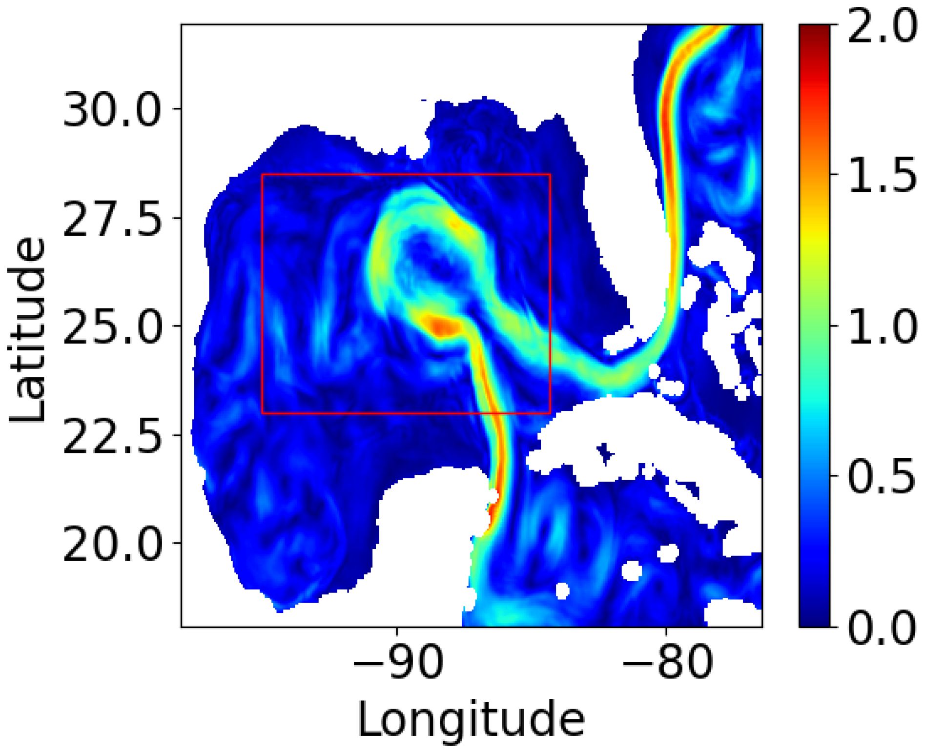
Figure 1. Velocity magnitude in ms⁻¹ snapshot on 1 October 2021 of the data assimilated numerical model. The red rectangle shows the region of interest used for the Physics Informed Neural Network evaluation.

Figure 2

Map showing the drift patterns in the Gulf of Mexico from October 1 to October 30, 2021, using OpenDrift. Green dots indicate initial positions, blue for active drifters, and red for stranded ones, with a total of 400 drifters tracked. Gray lines illustrate drift paths. The map is overlaid with latitude and longitude coordinates.

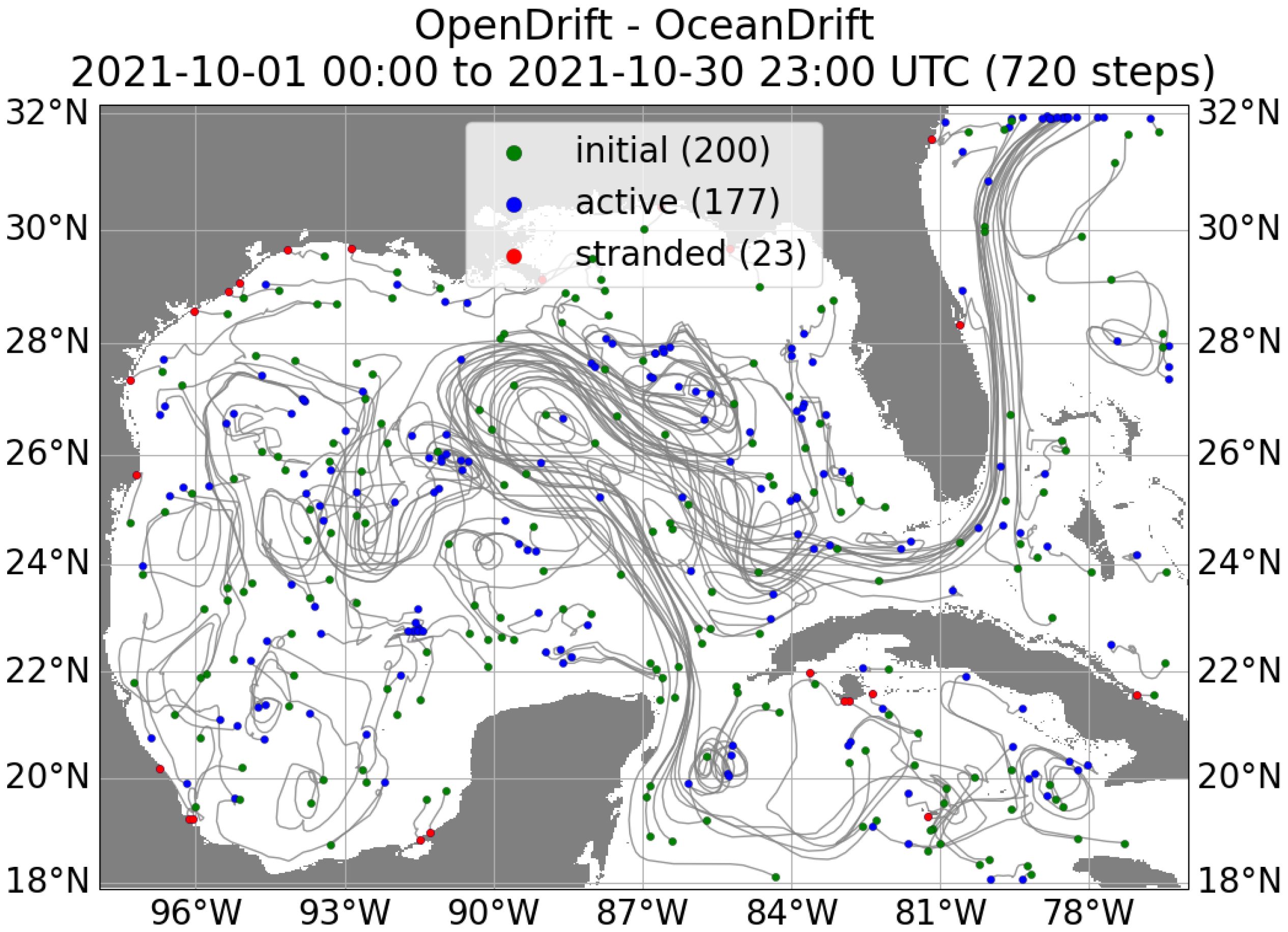
Figure 2. Trajectory of the 200 virtual drifters obtained from OpenDrift model. Green (blue) dots show the initial (final) positions and red dot the stranded position.

At synoptic scales, drifter-based reconstructions of surface velocity fields (influenced by both geostrophic and ageostrophic dynamics) are hampered, even over modest spatial regions, by a lack of contemporaneous drifter measurements with adequate spatial data density (Berta et al., 2015). Therefore, the number of drifters used in the reconstruction process will determine the accuracy of the reconstructed velocity field. A realistic number of drifters used in previous experiments such as LASER (Gonçalves et al., 2019), SPLASH (Lilly and Pérez-Brunius, 2021) or the Grand Lagrangian Deployment (Berta et al., 2015, GLAD) was about 300, which were deployed in a limited area of the GOM. While the PINN-SR method is first evaluated with 200 drifters (corresponding to a total of 144000 data points), the effect of the number of drifters on the accuracy of the reconstructed field was also evaluated by varying their numbers from 25 to 500 with a 25 increment from 25 to 200 and a 50 increment from 200 to 500. This sensitivity analysis will provide the number of drifters at which point the performance of the PINN-SR method plateaus. The initial drifter positions were randomly selected in the GoM region.

2.2 Drifter deployments in the Gulf of Mexico for operational purpose

For offshore operators, navigating the GoM and the waters from Trinidad to Brazil presents unique challenges, especially with strong ocean currents such as the LC and the North Brazil Current. The Woods Hole Group EddyWatch^® service provides a vital solution, offering comprehensive monitoring and forecasting of these powerful currents to ensure safety, reduce nonproductive time, and support operational efficiency. In particular, advanced data collection and analysis is conducted with satellite-tracked drifting buoys. The Far Horizon Drifter (FHD) is an air-deployable, satellite-tracked buoy composed of a cylindrical canister at the surface that transmits GPS coordinates hourly and a 45 m tether connected to a drogue. Ten units are deployed every two weeks in the central GoM in addition to custom deployments for specific operators. EddyWatch^® provides real-time data on current speed, direction, and key ocean phenomena. This data provides deep insight into how currents evolve and affect specific lease areas, enabling operators to adapt quickly to changing conditions. For the purpose of this study, Woods Hole Group provided 119 individual drifter trajectories over the period 31 July 2021 00:00:00–27 November 2021 23:00:00, corresponding to 120 days. This dataset consists of a total of 150568 records averaging 1265 records per drifter, equivalent to 52.7 days per drifter. Throughout the time range, the drifter locations were comprised between 97.22 and 53.68°W and 6.78 and 37.25°N. u and v varied between −4.78 and 4.59m.s⁻¹, and between −4.94 and 4.88m.s⁻¹ respectively. Only drifter trajectories located inside the GoM for the entire time range (Figure 3), which resulted in a total of 98763 records, were used for this study. In order to provide sufficient data points for the model to converge, the entire time period of the deployment was necessary.

Figure 3

Map titled “Drifter Paths in the Gulf of Mexico” shows real drifter trajectories with initial positions marked by green dots and final positions by blue dots. Lines connect these points, illustrating movement patterns. The map covers coordinates from 97.5°W to 80°W and 20°N to 30°N.

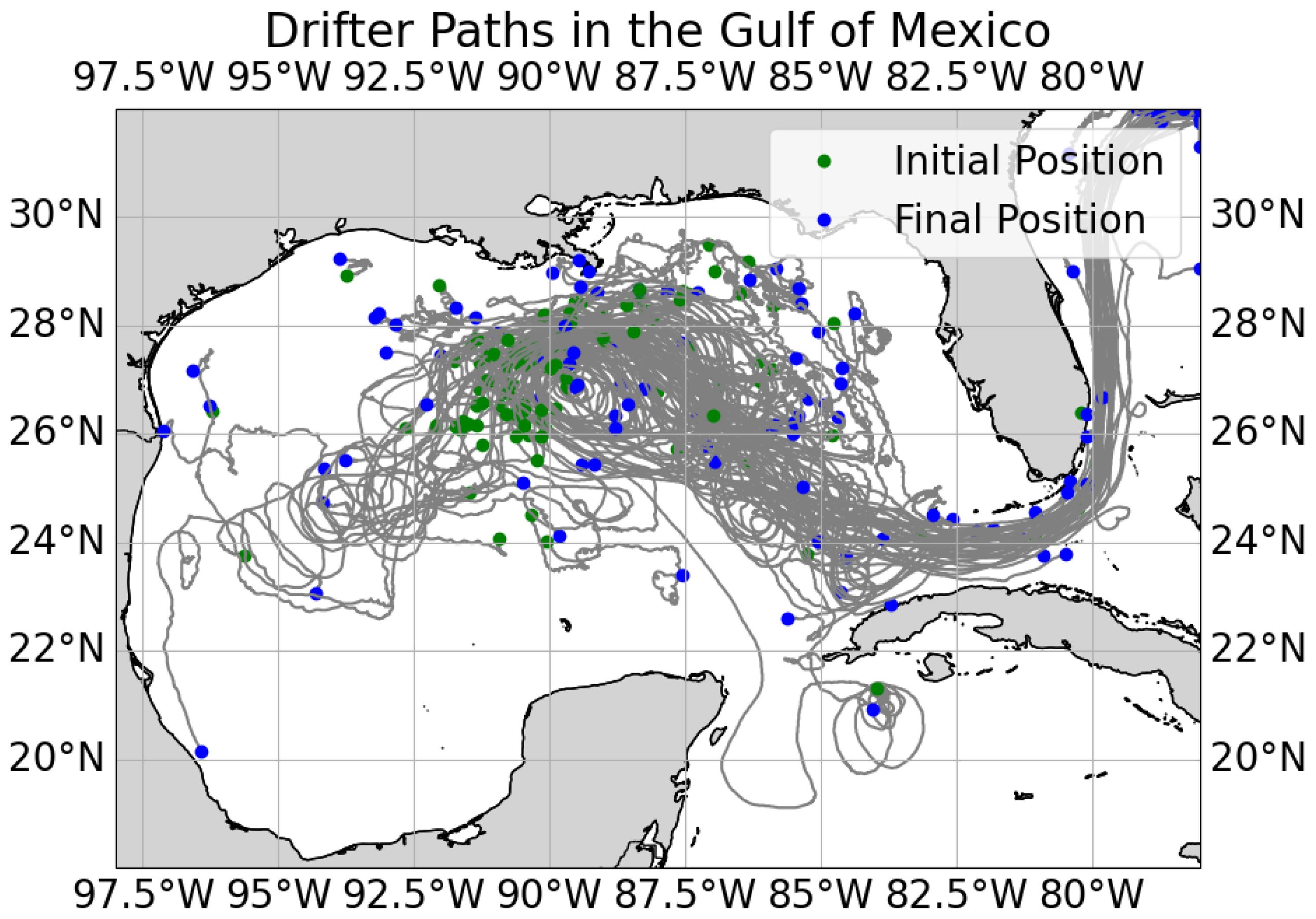
Figure 3. Distribution of Woods Hole Group’s drifters in the Gulf of Mexico over the period 31 July 2021 00:00:00–27 November 2021 23:00:00.

2.3 Data augmentation

In order to extend the footprint of each drifter trajectories, both in time and space, we applied a data augmentation technique. Data augmentation is a technique to increase the quantity and variability of the training samples. To do so, we first gridded the drifter locations on the same grid as the resampled numerical model fields to have a uniform resolution across the dataset. The velocity in a grid cell was obtained by averaging the velocity of all the drifter points in that cell. Then, we performed two types of augmentation, one in space and one in time. The spatial augmentation is grounded in the fact that the velocity does not change much within a certain radius and, in this case, around a drifter position, as suggested by the integral timescale estimation of Mariano et al. (2016) in the GoM. Twice the integral time scale is the time for velocity measurements to become independent; It is fundamental for estimating the effective degree of freedom in a correlated velocity data set and determining how long a Lagrangian motion prediction is reliable. In the northeast GoM, Mariano et al. (2016) estimated an average integral time scale of 1 day. Let’s consider a point $P (x_{t_{k}}^{k}, y_{t_{k}}^{k})$ , k^th point on the trajectory of a drifter, recorded at time t_k. Assuming an average drifter velocity of 0.1 m.s⁻¹ yields the surrounding points in a radius r = 0.08° have the same velocity as P, resulting in eight additional points (Figure 4A).

Figure 4

Diagram comparing data before and after augmentation. Panel A shows a cluster of blue dots within a dashed circle labeled $ P(x^k_{t_k}, y^k_{t_k}) $. Panel B illustrates three separate dots labeled $ P(x^k_{t_k}, y^k_{t_k}) $, $ P1(x^{k+1}_{t_k}, y^{k+1}_{t_k}) $, and $ P2(x^{k+2}_{t_k}, y^{k+2}_{t_k}) $, signifying data after augmentation.

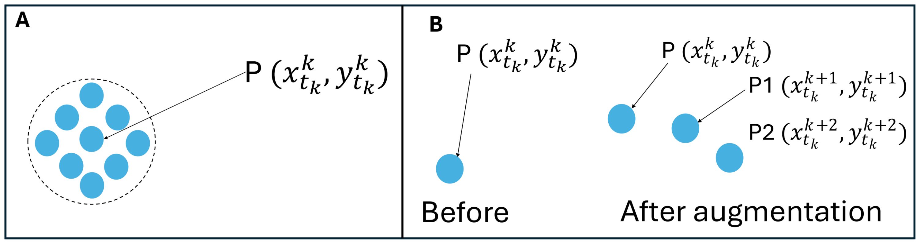
Figure 4. Spatial (A) and temporal (B) augmentation concept. In (A) the spatial augmentation is grounded in the fact that the velocity does not change much within a certain radius. In (B) the velocity at a given location will be the same over a given time period, hence $P (x_{t_{k}}^{k}, y_{t_{k}}^{k}) = P 1 (x_{t_{k} + 1}^{k}, y_{t_{k} + 1}^{k}) = P 1 (x_{t_{k}}^{k + 1}, y_{t_{k}}^{k + 1})$ . $P (x_{t_{k}}^{k}, y_{t_{k}}^{k})$ is the k^th point on the trajectory where $x_{t_{k}}^{k}$ and $y_{t_{k}}^{k}$ are the coordinates of the drifter at time t_k.

The temporal augmentation is based on the fact that the velocity does not change much over time for nearby points, as inferred from the e-folding time scale of less than 12 hours calculated by Mariano et al. (2016) in the northeast GoM. For the point $P (x_{t_{k}}^{k}, y_{t_{k}}^{k})$ , we assume that the velocity of the points located in the same position as N future points (with corresponding time t_k₊₁,t_k₊₂,…,t_k₊_N) on the drifter’s trajectory is the same as the velocity of those future points but for the current time t_k. We chose N = 9 in our experiments, which is equivalent to the next 9 hours due to the hourly resolution of the drifter positions (Figure 4B).

Figure 5 shows a complete example of the augmentation carried out on a sample point. Figure 5A shows a sample position on a drifter trajectory. It first goes through temporal augmentation (Figure 5B) and then through spatial augmentation (Figure 5C). When applied to the whole trajectory (Figure 5D), the resulting augmentation is shown in Figure 5E. The colors show the magnitude of the velocity, which remains consistent with the original trajectories after the augmentation.

Figure 5

Five scatter plots labeled A to E, showing data points with latitude and longitude coordinates. Color gradients from blue to red represent varying data values. Plots A to C show clustered points in a small range, while plots D and E depict more extended, curving paths across wider geographic areas, indicated by the different scales and color bars.

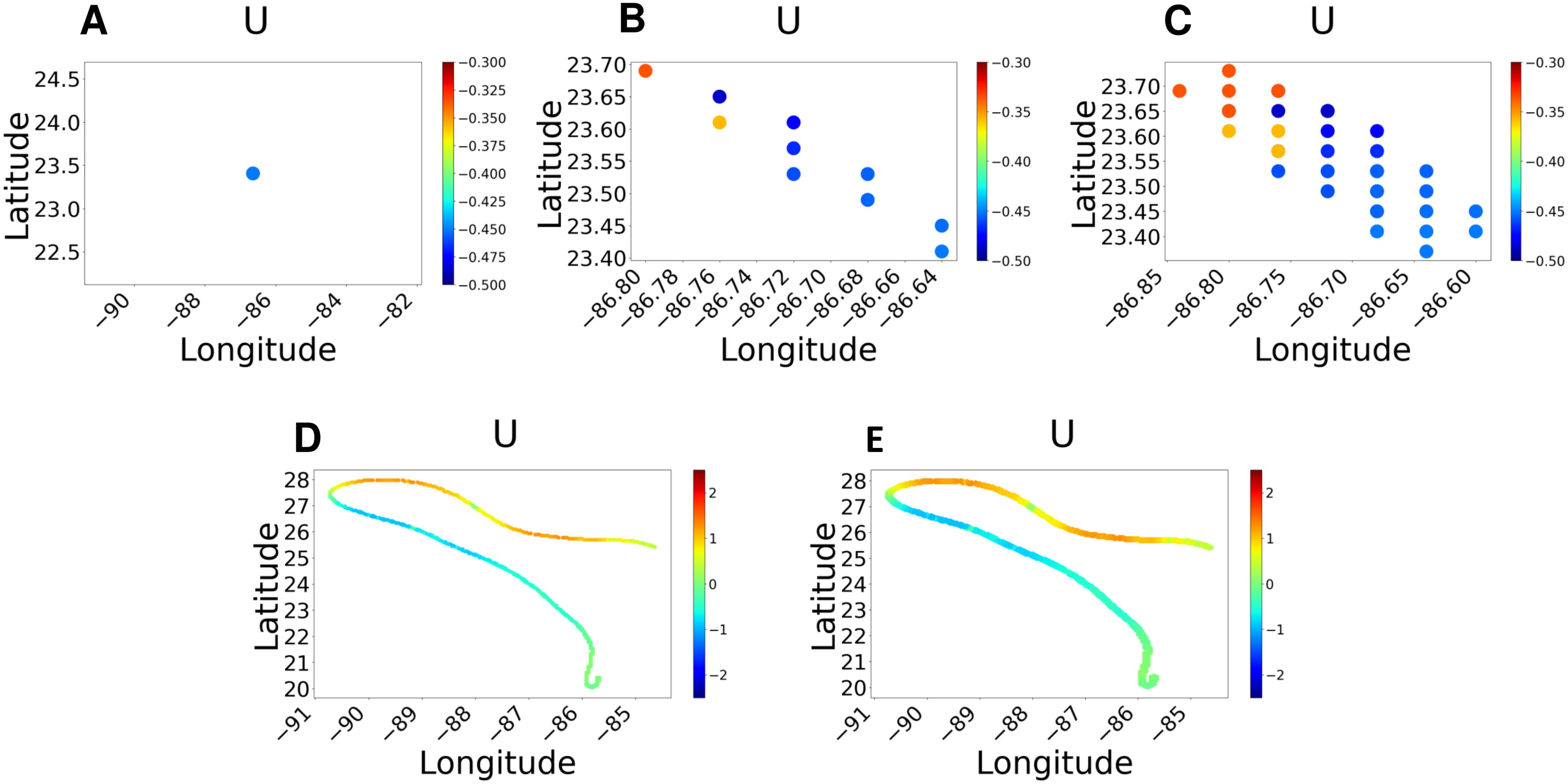
Figure 5. Data augmentation procedure. (A) A point in a drifter’s trajectory, (B) the result of its temporal augmentation, and (C) the output of (B)’s spatial augmentation. (D) shows a drifter trajectory and (E) the augmented data from the trajectory in (D). Colors show the velocity values (m.s⁻¹) at each location. Dots in (A–C) have been enlarged for visibility.

2.4 Physics-informed neural network with sparse regression

PINN has been proposed as an alternative to classical numerical methods, such as finite element methods (FEM), to solve ordinary and partial differential equations (ODE and PDE, respectively). Raissi et al. (2019) showed that PINN can help solve the forward and inverse problems of PDEs. PINN can also be used to uncover differential equations describing a physical phenomenon by adding a loss that encompasses the residual of the differential equation. However, SR is a regression technique that reduces the number of parameters in a model while maintaining a satisfying performance. In our approach, we apply the PINN-SR method proposed by Chen et al. (2021) to reconstruct the velocity field and extract the PDE that governs the movement of water. Chen et al. (2021) used PINN-SR to uncover the Navier-Stokes equations, which are the governing equations of oceanic flows, which govern drifter trajectories. The SR is crucially important because it promotes sparsity for the coefficients of the uncovered differential equations. The equations are encoded in the loss function, which improves the learning process that is not only data driven but also physics driven, and in this case by the geophysical fluid dynamics. SR is also designed to handle the data sparsity and noise inherent to drifter data.

The PINN-SR framework is shown in Figure 6. It relies on a dense (fully connected) DNN that is chosen here as the Mutli-layer Perceptron (MLP). MLP is a modern feedforward artificial neural network, consisting of fully connected neurons with a nonlinear activation function, organized in at least three layers, notable for being able to solve problems requiring non-linear solutions (Cybenko, 1989). The input to the PINN-SR consists of the coordinates and time (x,y,t) of the drifter positions fed to the MLP. The output of the MLP is the velocity vector u = (u,v). Then u is passed through the auto-differentiation module that computes the derivatives w.r.t. x, y, and t. u, v, and their derivatives are used to form the library of candidate terms that can be constant, polynomial, or trigonometric functions. The assumption is that the PDE can be reconstituted by combining those candidate terms. The matrix Λ contains the coefficients of the candidate functions. Λ is a sparse matrix in which sparsity is promoted using Sparse Regression. The goal is to reconstitute the PDE with as few coefficients as possible while maintaining its closeness to the system’s dynamics. Given the complexity of this optimization problem, Alternative Direction Optimization (ADO) was applied. ADO seeks to determine the optimal Λ values that minimize the sparse regression loss (achieved by STRidge, Figure 6) and the optimal θ weights that minimize the loss (achieved with Adam, Figure 6). The MLP weights θ are optimized while the SR weights are fixed, that is, the elements of Λ. Then, θ is frozen and Λ optimized. The loss function has three terms. The first term is the data loss L_d(θ; D_u), the second the physics loss L_p(θ, Λ; D_c) and the third the regularization term $∥ Λ ∥_{0}$ ¹.

Figure 6

Flowchart depicting a process involving machine learning. Stages include “MLP with Unknown Parameters,” featuring an MLP with inputs $t$, $x$, $y$. “Auto differentiation” follows, showing differentiation nodes and function selection. “PDE Construction” involves constructing equations with matrices and sparse representation. “Sparse Regression” shows solving for unknown parameters $\Lambda$. Equations at the bottom indicate loss calculations and iterative solution updates using ADO and STRidge.

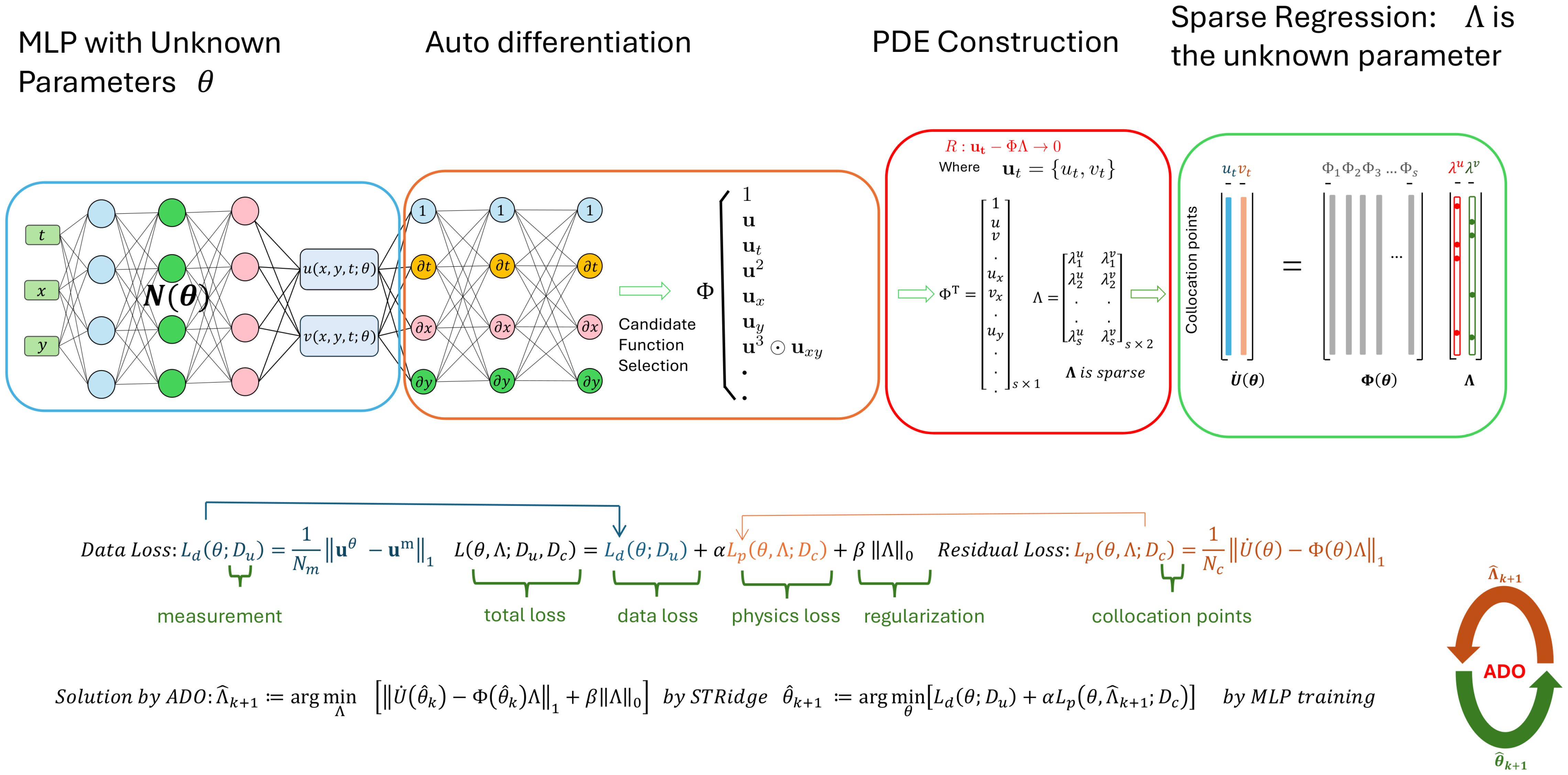
Figure 6. PINN-SR framework proposed by Chen et al. (2021). The Multi-Layer Perceptron (MLP - blue block) input is (x,y,t) and outputs are the velocity components u and v. Then, the auto differentiation (orange block) module computes the derivatives (first, second, third order, etc., depending on the data’s complexity) of u and v w.r.t. x,y,t. The candidate functions are computed using u, v, and their derivatives. For example, u_t and u_x represent the first-order derivatives w.r.t. t and x respectively. The formed candidate functions are regrouped into Φ, which will be used to reconstruct the PDE, whose residual, u_t − ΦΛ, should tend toward zero (red block). Λ coefficients are obtained using Sparse Regression (SR green block) on the collocation points. The formulation of the loss function is provided in the first equation. The formulation of the Alternative Direction Optimization (ADO) is given in the second equation. N_m and N_c represent the number of measurements (data) and collocation points, respectively.

It is important to note that the data loss is computed using the measurement data D_u(corresponding to drifters data in this case), while the physics loss uses collocation points ² D_c. α and β represent weight coefficients (Figure 6). PINN-SR training involves two stages: the pre-training stage and the ADO stage. The pretraining stage focuses on giving prior knowledge to the neural network before engaging in the ADO stage, which allows the improvement of the neural network and the discovery of the differential equation alternatively. For pretraining, stochastic optimizers such as stochastic gradient descent (SGD) Robbins and Monro (1951), Adam Kingma (2014), and others can be used, followed by a deterministic algorithm such as limited-memory Broyden-Fletcher-Goldfarb-Shannon (LBFGS) Liu and Nocedal (1989). In the ADO stage, only a stochastic optimizer is used to optimize the weights of the neural network. For a more detailed discussion of the PINN-SR model, the reader is referred to Chen et al. (2021).

2.5 Training

We used an 80/20 data split for training and validation for all experiments. The MLP used has 8 hidden layers of 60 nodes each and 2 nodes for the output layer because the model predicts both u and v. We used the tanh activation function, which is widely used in PINN because, contrary to ReLU (Rectified Linear Unit (Nair and Hinton, 2010)), it has second-order derivatives. The optimizer used for the PINN-SR pre-training is Adam, with a learning rate of 5.10⁻³ for 10 000 iterations, followed by 40 000 LBFGS-B iterations. For the ADO stage, Adam is maintained but with a learning rate of 1e-3 for 1000 iterations. Six ADO iterations are performed in total. We trained the model on a single Nvidia Tesla V100 GPU of 32 GB of memory for about 6 hours and 15 minutes. We opted for the L1 loss instead of L2 because the latter tends to produce blurry results (Mathieu et al., 2015), thus removing the small-scale dynamics from the reconstructed field. Hyperparameters are summarized in Table 1.

Table 1

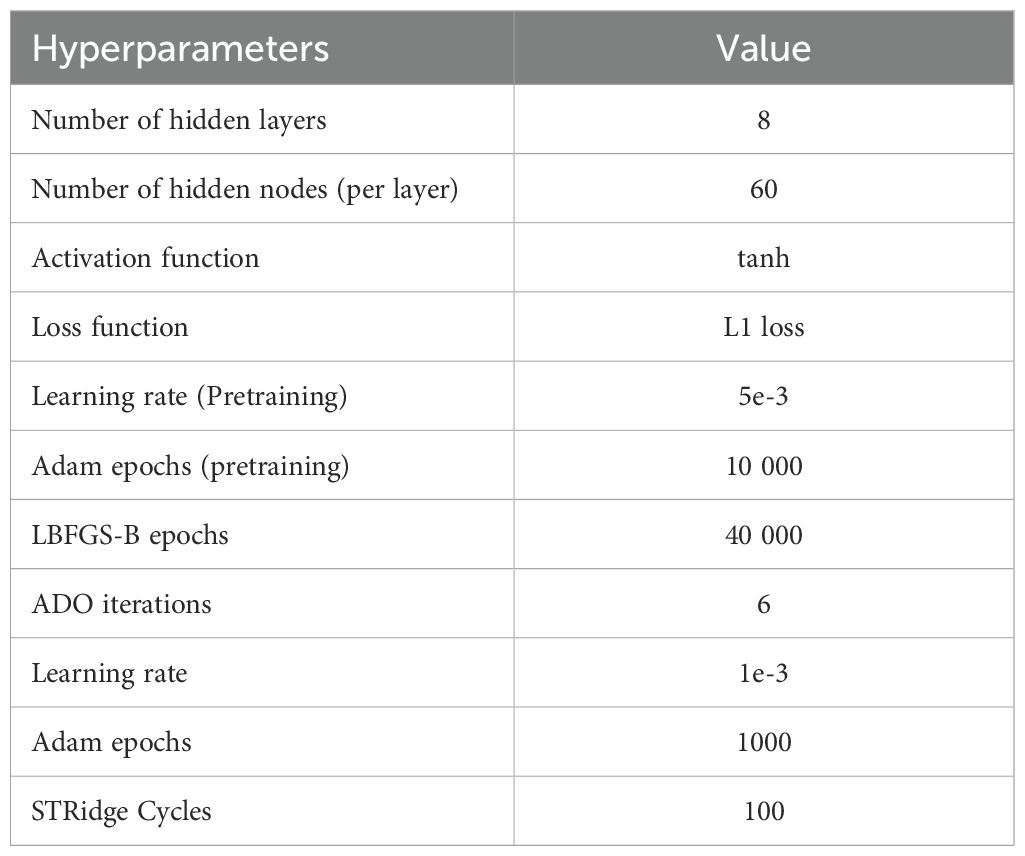
Table 1. Hyperparameter values used to train the PINN.

2.6 Deep neural network and field interpolation

To show the improvement of the PINN-SR approach, the velocity field was also reconstructed with a DNN without physics learning and traditional binning and interpolation methods. The DNN consisted of an MLP with 6 hidden layers of 60 nodes each, trained for 50 000 epochs with the same hyperparameters as in the PINN-SR model (Table 1). The binning and interpolation methods consist of the universalKriging [U-Kriging - (Krige, 1951)] and the inverse distance weighted (IDW) methods. They both used the same number of neighbors, 11, and a radius search of 0.04^°. IDW estimates the value at a desired location by computing the weighted average of the values of the neighboring points, the weights being the inverse distance between the desired location and the neighboring points. U-Kriging is also known as the Gaussian process regression where the spatial distribution of the observed data, their distance to the point of calculation and their spatial correlation are taken into account (Goovaerts and Authorid, 2019). These two methods form the basis for interpolation methods to fill in missing data (Kostopoulou, 2021) and even to correct spatial pattern biases in numerical models due to the spatial autocorrelation property (Chang et al., 2021).

2.7 Evaluation of models performance

We use qualitative and quantitative approaches to assess the performance of our models. The qualitative assessment consists of a visual comparison of the velocity field of the PINN-SR model output and the numerical model. For quantitative assessment, we used RMSE and CC, and MS-SSIM for image similarity analysis (Wang et al., 2003, 2004). RMSE is the point-to-point difference between the predicted and reference fields. The result is a positive real number used to estimate how similar in magnitude the two fields are and is given by:

RMSE = \sqrt{\frac{1}{n . m} \sum_{i = 1}^{n} \sum_{j = 1}^{m} {(I_{i j} - {\hat{I}}_{i j})}^{2}},

where n is the number of rows, m is the number of columns, I_ij is the element of the reference field I at position (i,j), ${\hat{I}}_{i j}$ is the element of reconstructed field $\hat{I}$ at position (i,j). Low RMSE values are indicative of reduced differences in magnitude between two fields.

CC measures the phase alignment between the predicted and reference fields and is expressed as follows:

CC (I, \hat{I}) = \frac{\sum_{i, j} (I_{i j} - \bar{I}) \cdot ({\hat{I}}_{i j} - \bar{\hat{I}})}{\sqrt{\sum_{i, j} {(I_{i j} - \bar{I})}^{2}} \cdot \sqrt{\sum_{i, j} {({\hat{I}}_{i j} - \bar{\hat{I}})}^{2}}},

where $\bar{I}$ and $\bar{\hat{I}}$ are the mean values of the arrays I and $\hat{I}$ , respectively. Phase alignment is reached when CC = 1.

MS-SSIM is used to quantify the similarity between the velocity field arrays, considered here as images. This index was originally developed to assess image quality by quantifying differences between signals from distorted and reference images and can simultaneously consider accuracy, precision, and spatial similarities at multiple scales (Wang et al., 2003, 2004). It can be written as follows.

MS - SSIM (I, \hat{I}) = \frac{1}{L} \sum_{l = 1}^{L} [(\frac{2 μ_{I_{l}} μ_{{\hat{I}}_{l}} + c_{1}}{μ_{I_{l}}^{2} + μ_{{\hat{I}}_{l}}^{2} + c_{1}}) \cdot (\frac{2 σ_{I_{l} {\hat{I}}_{l}} + c_{2}}{σ_{I_{l}}^{2} + σ_{{\hat{I}}_{l}}^{2} + c_{2}}) \cdot (\frac{σ_{I_{l} {\hat{I}}_{l}} + c_{3}}{σ_{I_{l}} σ_{{\hat{I}}_{l}} + c_{3}})]^{α_{l}}

L is the number of levels in the decomposition, $μ_{I_{l}}$ and $μ_{{\hat{I}}_{l}}$ are the means of I and $\hat{I}$ at level l, $σ_{I_{l}}^{2}$ and $σ_{{\hat{I}}_{l}}^{2}$ are the variances of I and $\hat{I}$ at level l, $σ_{I_{l} {\hat{I}}_{l}}$ is the covariance between I and $\hat{I}$ at level l, c₁, c₂, and c₃ are small constants to prevent division by zero or very small denominators, α_l are weights for the components at level l. MS-SSIM varies between 0 and 1 where the latter indicates identical fields.

To evaluate the performance of the real drifters’ reconstructed field, several datasets were used, including model and observations. The reconstructed velocity field was first converted to velocity contours of the 0.7 m.s⁻¹ isotach, which is the critical velocity watched by offshore operators. Those contours were compared to the location of circulation features in the DA model SSH and 0.7 m.s⁻¹ isotach. One kilometer resolution chlorophyll-a imagery from the MODIS sensor obtained from the Optical Oceanography Observatory at University of South Florida were use to validate the presence of small scale circulation features in the flow present in the reconstructed velocity field.

3 Results

3.1 Virtual drifters velocity field reconstruction

The performance of the PINN-SR model is evaluated in terms of the comparison of the reconstructed velocity field with the DA model velocity field. The overall metrics assessment is conducted over the period 1–30 October 2021 and is summarized in Table 2 for the zonal and meridional components of the velocity vector, respectively. Overall, the PINN-SR method performs significantly better than the MLP, IDW, and U-Kriging. The RMSE of the PINN-SR method is 40% less than that of the U-Kriging and IDW methods and 33% less than that of the MLP. The CC between the reference and the PINN-SR reconstructed fields is 18% higher than with IDW and U-Kriging and 11% higher than with MLP. MS-SSIM is 11.6% higher for PINN-SR model than the latter three. Furthermore, the standard deviation of the PINN-SR method is significantly smaller than that of the other three methods for all metrics.

Table 2

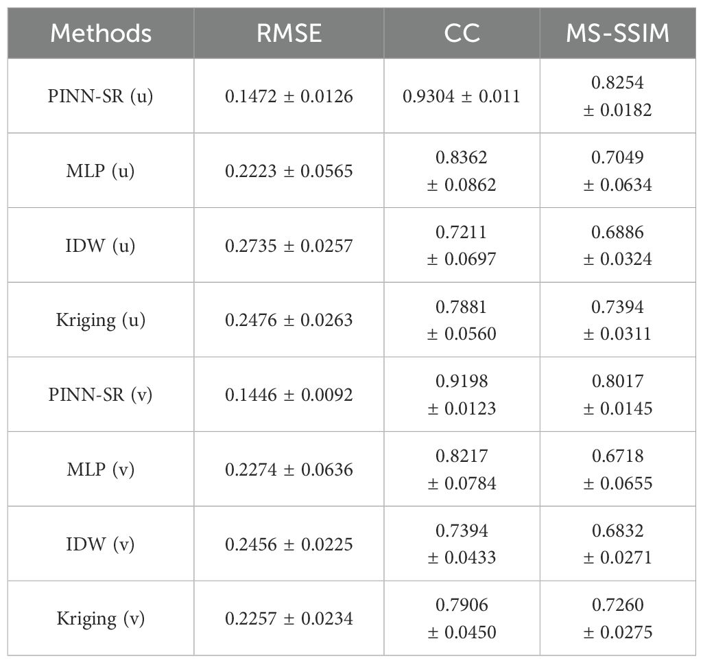
Table 2. Mean and standard deviation of the skill metrics RMSE (m.s⁻¹), CC and MS-SSIM for velocity components u and v, respectively, computed between 1–30 October 2021.

The temporal evolution of the three metrics, for each method, reveals that they vary over time, especially for the U-Kriging and IDW methods (blue and green lines in Figure 7). The metrics for the PINN-SR method exhibit smaller relative variations overall and indicate temporal stability and superior performance of the method over MLP, U-Kriging and IDW. A slight increase of the RMSE, decrease of CC and MS-SSIM can be seen at the end of the testing period, in this particular case. The MLP’s reconstructed field metrics suggest that MPL alone is not as efficient at reconstructing the Eulerian velocity field as the PINN-SR method, especially the meridional velocity field (Figures 7D–F). This result indicates the significant role of the physics-learning part of the algorithm in the reconstruction of the velocity field.

Figure 7

Six line graphs comparing four methods: PINN, MLP, IDW, and Kriging over 30 days. Graph A shows RMSE for “u

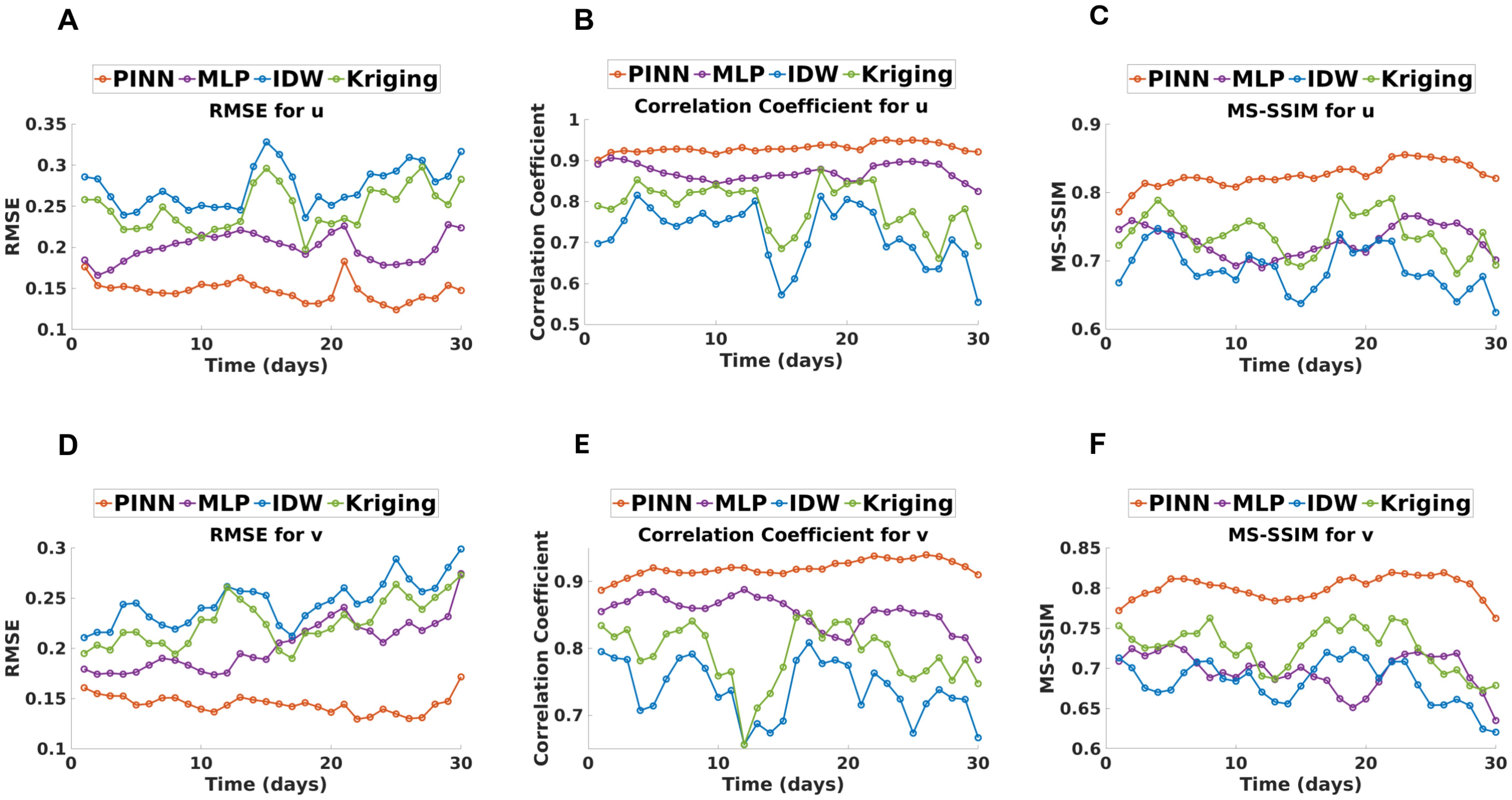
Figure 7. Time evolution from 1–30 October 2021 of RMSE (m.s⁻¹) (A, D), CC (B, E), and MS-SSIM (C, F) for u and v (first and second row respectively) calculated on the region of interest (Figure 1) for the PINN-SR (orange line), the MLP (purple line), the IDW (blue line) and, the Kriging methods (green line). Day 1 is 1 October 2021.

Snapshots of the velocity field (Figures 8, 9) show that the PINN-SR method is capable of reproducing all the features of the velocity fields for the u and v components in terms of location, shape, and magnitude, unlike the U-Kriging and IDW methods. The MLP alone is also capable of capturing the same features of the original velocity field; however, the differences with the PINN-SR reconstructed fields lie in the misalignment of the flow features by MLP as shown in Figure 10, which the MS-SSIM suggests (Table 2). Resolving the underlying physics of the velocity field through its differential equations appears to significantly improve the flow feature dynamics captured by the Lagrangian field.

Figure 8

Graphical representation showing current speed or heat maps data comparisons over seven days from October 1 to October 7, 2021. Each day has five visualizations labeled “Ground Truth,” “PINN,” “MLP,” “Universal Kriging,” and “IDW,” displaying color-coded data from blue to red. Latitude and longitude coordinates are shown with a color bar range of -2 to 2 on the right.

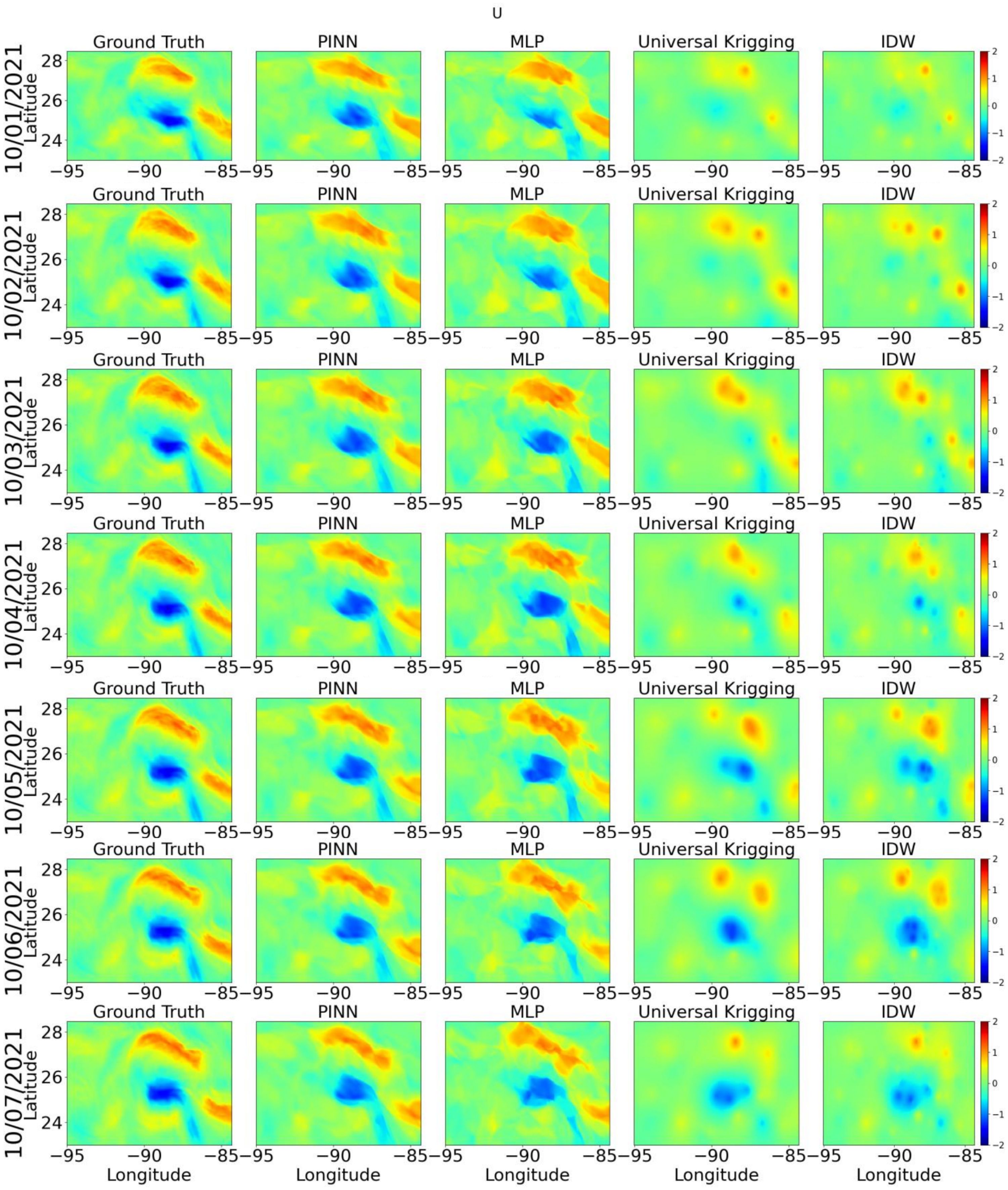
Figure 8. Reference and reconstructed velocity fields (m.s⁻¹) shown by rows of five for the zonal velocity u. From the left to right, is shown the numerical model field, the PINN-SR, MLP, Universal Kriging, and IDW reconstructed field. Each row represents a day from 1–7 October 2021.The x-axis represents the longitude and the y-axis the latitude. The date is shown on the y-axis as well.

Figure 9

Heatmaps displaying geographical data from October 1 to October 7, 2021. Each row represents a day with five columns labeled Ground Truth, PINN, MLP, Universal Kriging, and IDW. The color scale ranges from blue (low values) to red (high values) with coordinates spanning latitudes 24 to 28 and longitudes -95 to -85.

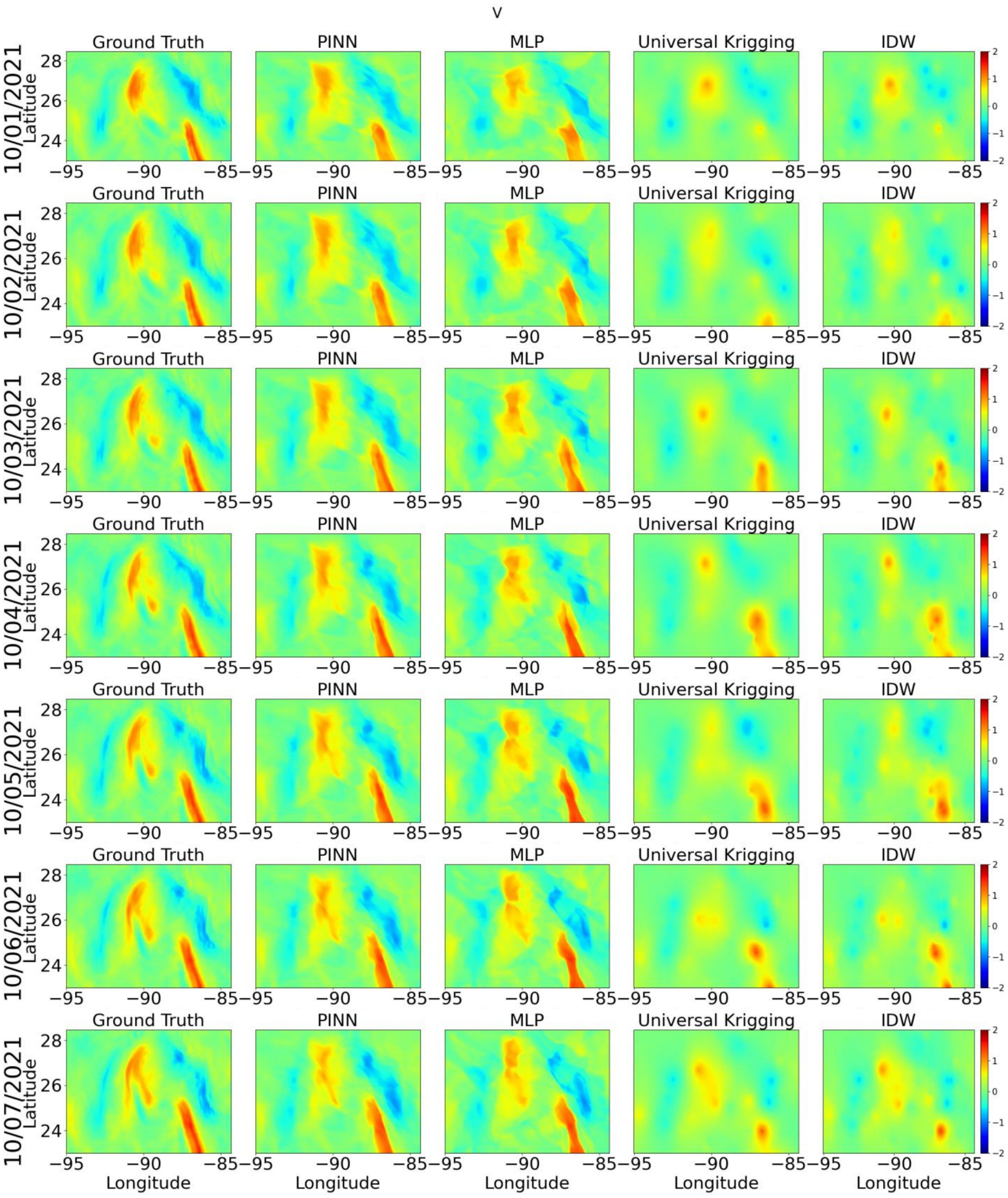
Figure 9. Reference and reconstructed velocity fields (m.s⁻¹) shown by rows of five for the meridional velocity v. From the left to right, is shown the numerical model field, the PINN-SR, MLP, Universal Kriging, and IDW reconstructed field. Each row represents a day from 1–7 October 2021. The x-axis represents the longitude and the y-axis the latitude. The date is shown on the y-axis as well.

Figure 10

Twelve heatmaps show differences between predictions from a neural network and a baseline MLP model for U and V components over several days in October 2021. Each map is labeled with a date ranging from October 1 to October 7, with axes representing latitude and longitude. A color scale to the right indicates values from minus two to two.

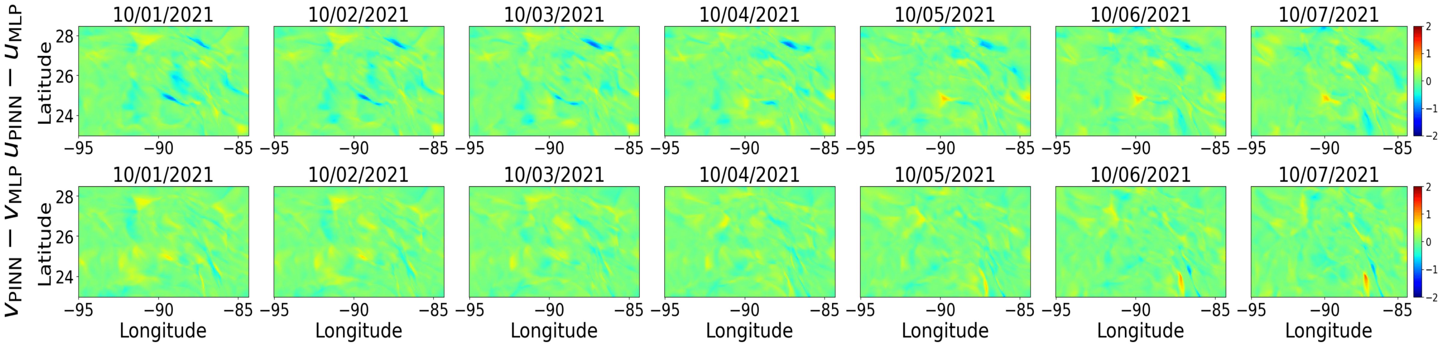
Figure 10. Difference between PINN-SR and MLP reconstructed velocity fields (m.s⁻¹) shown by rows of seven for the zonal (meridional) velocity u (v). Each column represents a day from 1–7 October 2021.The x-axis represents the longitude and the y-axis the latitude.

3.2 Effect of the number of drifters on the reconstructed field

In this section, we evaluate the performance of the PINN-SR based on the number of virtual drifters used for training. The reconstructed field is evaluated in terms of RMSE, CC, and MS-SSIM for each number of drifters as shown in Table 3, which also shows the number of drifters per sq. degree.

Table 3

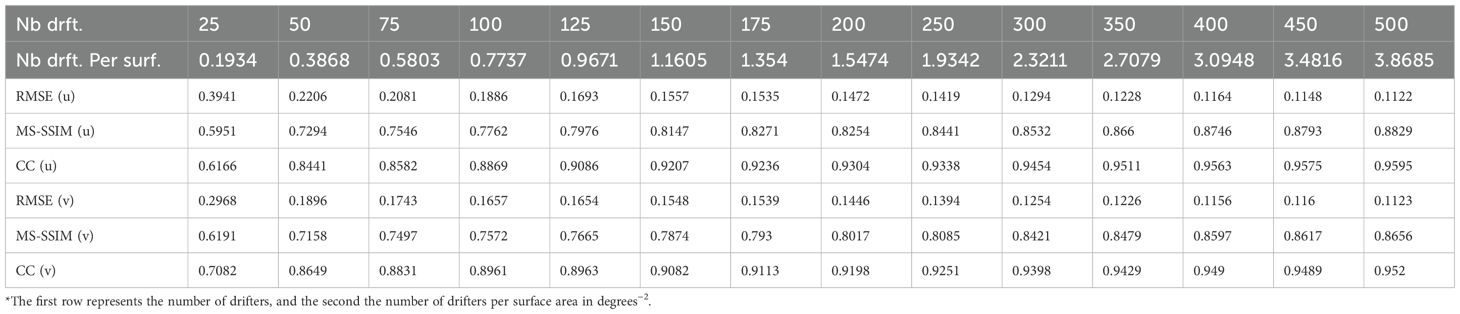
Table 3. PINN-SR metrics evolution with the number of drifters used for training*.

The evolution of the three metrics versus the number of drifters is captured in Figures 11A–C showing the RMSE, the CC, and the MS-SSIM, respectively. For all three metrics, doubling the number of drifters from 25 to 50 shows a rapid improvement in the reconstructed field. As the number of drifters increases, the improvement tends to slowly plateau. The improvement in RMSE becomes less than 10% between 255–300 and 500 drifters versus 60% between 25 and 250 drifters. For the CC, the change is from 1% versus 30%, and for the MS-SSIM, the change is 3.5% versus 42%, respectively. These results suggest that for an ocean basin like the GoM, the minimum number of drifters randomly seeded in the GoM that is necessary to properly reconstruct the velocity field with the PINN-SR method is between 200 and 300, which is the range of the number of drifters used in the most extensive recent drifter experiments in the GoM such as GLAD, LASER and CODE (Berta et al., 2015).

Figure 11

Graphs labeled A, B, and C show relationships between the number of drifters and three metrics: RMSE, Correlation Coefficient, and MS-SSIM. Graph A shows RMSE decreasing as drifters increase. Graph B shows the Correlation Coefficient increasing and plateauing. Graph C shows MS-SSIM generally increasing. Blue and orange lines represent datasets labeled “u” and “v”.

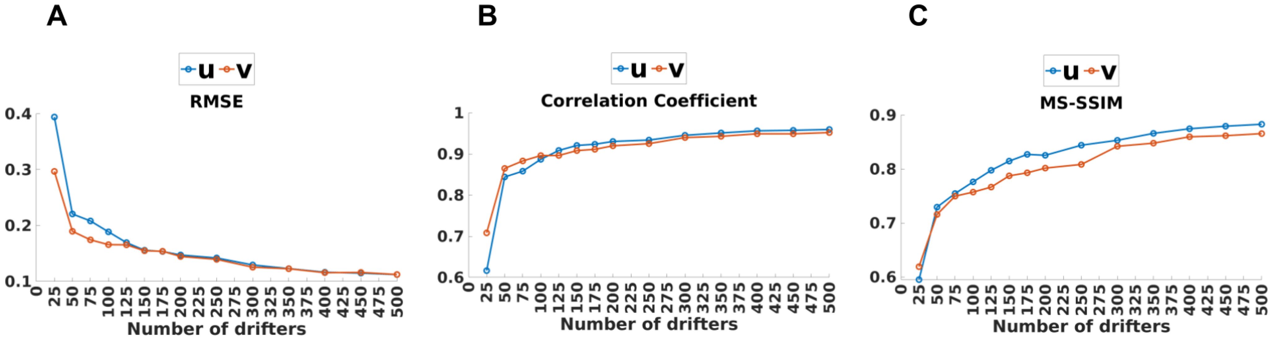
Figure 11. Evolution of the RMSE (A, m.s⁻¹), CC (B), and the MS-SSIM (C) between the PINN-SR reconstructed field and the DA numerical model output as a function of the number of virtual drifters used for training.

3.3 Application to real drifters trajectories

The reconstructed field from the Woods Hole Group drifter data for the period 6–8 November 2021 is shown in Figure 12, which falls during the testing period of the real drifter data. To evaluate the reconstructed field, the circulation features associated with the 0.7 m.s⁻¹ isotach were outlined on the 07 November 2021 velocity field of the DA model (Figure 13a) and on the reconstructed field (Figure 13b). In addition, the contour generated by EddyWatch^® was also made available to this study and is shown in Figures 13a, b. The EddyWatch^® generated contour only outlines the external velocity contour of the LC system and marks the presence of counter-rotating mesoscale eddies around the LC and the LC ring Eddy Verne in the western GoM. The external isotach of the DA model is relatively close in position to the EddyWatch^® contour (Figure 13a), which is derived from a combination of observations and numerical model output that include the DA model used in this study. The isotachs from the reconstructed field PINN-SR show a more complex pattern that encompasses the adjacent counter-rotating structures (Figure 13b) which are resolved by the DA model as shown by the SSH contours in Figure 13c. In particular, the cylconic circulation west of the LC is shown to exhibit higher velocities than what the DA model achieved. This result would suggest that the DA model underestimates the velocity field outside the main flow region of the LC as shown by the drifter location (red dots) that exhibits a speed at that location equal to 0.7 ms⁻1. The isotachs of the PINN-SR reconstructed field outline small-scale energetic features that are visible in the MODIS chlorophyll-a image on the same day as shown by the red circles in Figure 13d. The isotaches also outline velocity contours within existing structures outside the LC that are visible in the MODIS image.

Figure 12

Six-panel grid of maps titled “PINN Reconstructed Field” showing U and V components of a field over a geographic area from November 6 to 8, 2021. Each panel indicates variations in intensity from negative four to four, using color gradients from blue to red. Latitude ranges from 20 to 30 and longitude from -95 to -80.

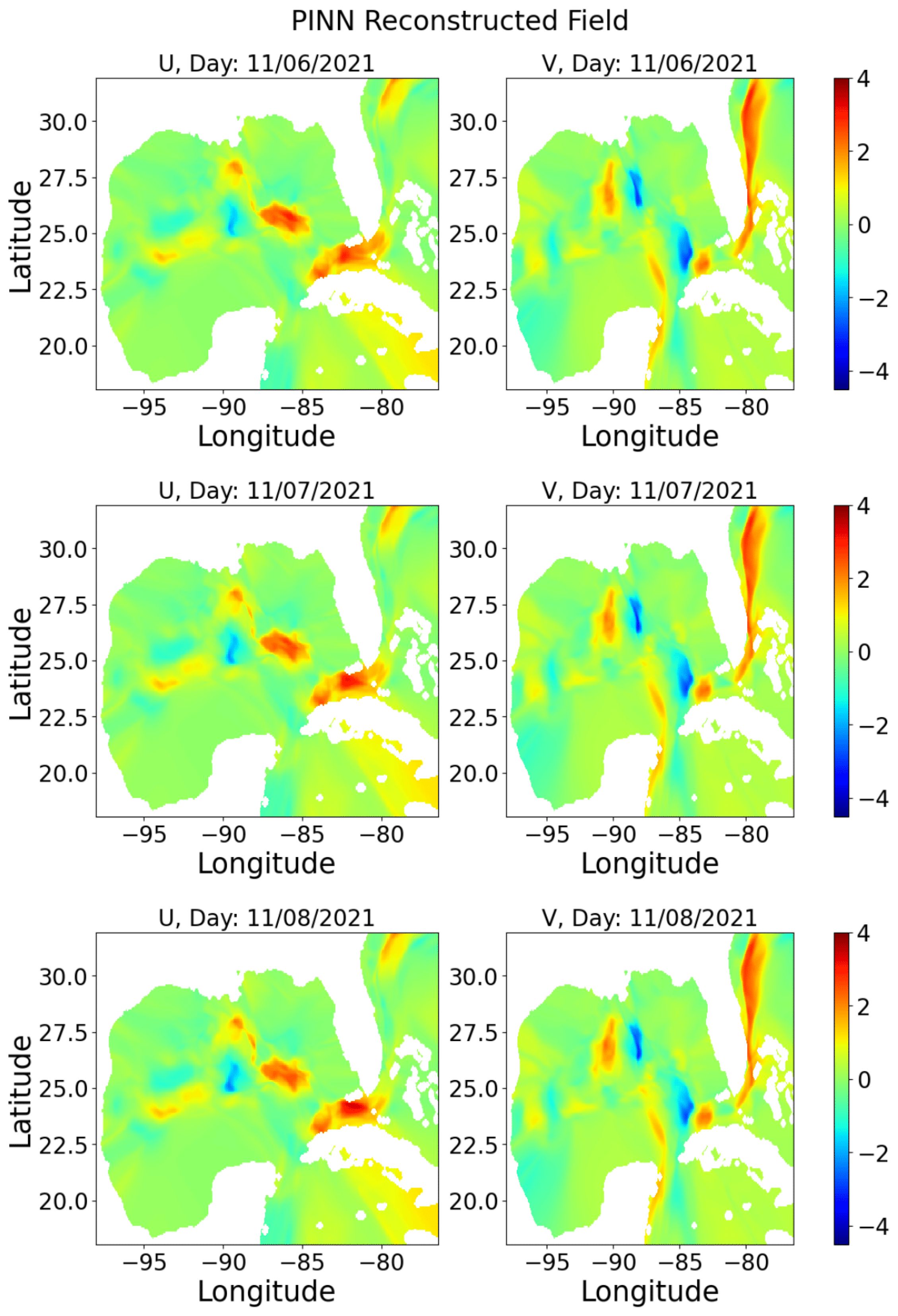
Figure 12. Reconstructed field for the period 6–8 November 2021 over three rows. The left (right) column shows the zonal (meridional) velocity.The x-axis represents the longitude and the y-axis the latitude.

Figure 13

Five maps show the Gulf of Mexico's sea surface conditions and currents on November 7 and 10, 2021. Each map presents contour lines and colored overlays representing different aspects of the ocean's surface such as currents, sea surface height and chlorophyll. Labels indicate longitude, latitude, specific currents, and gyres.

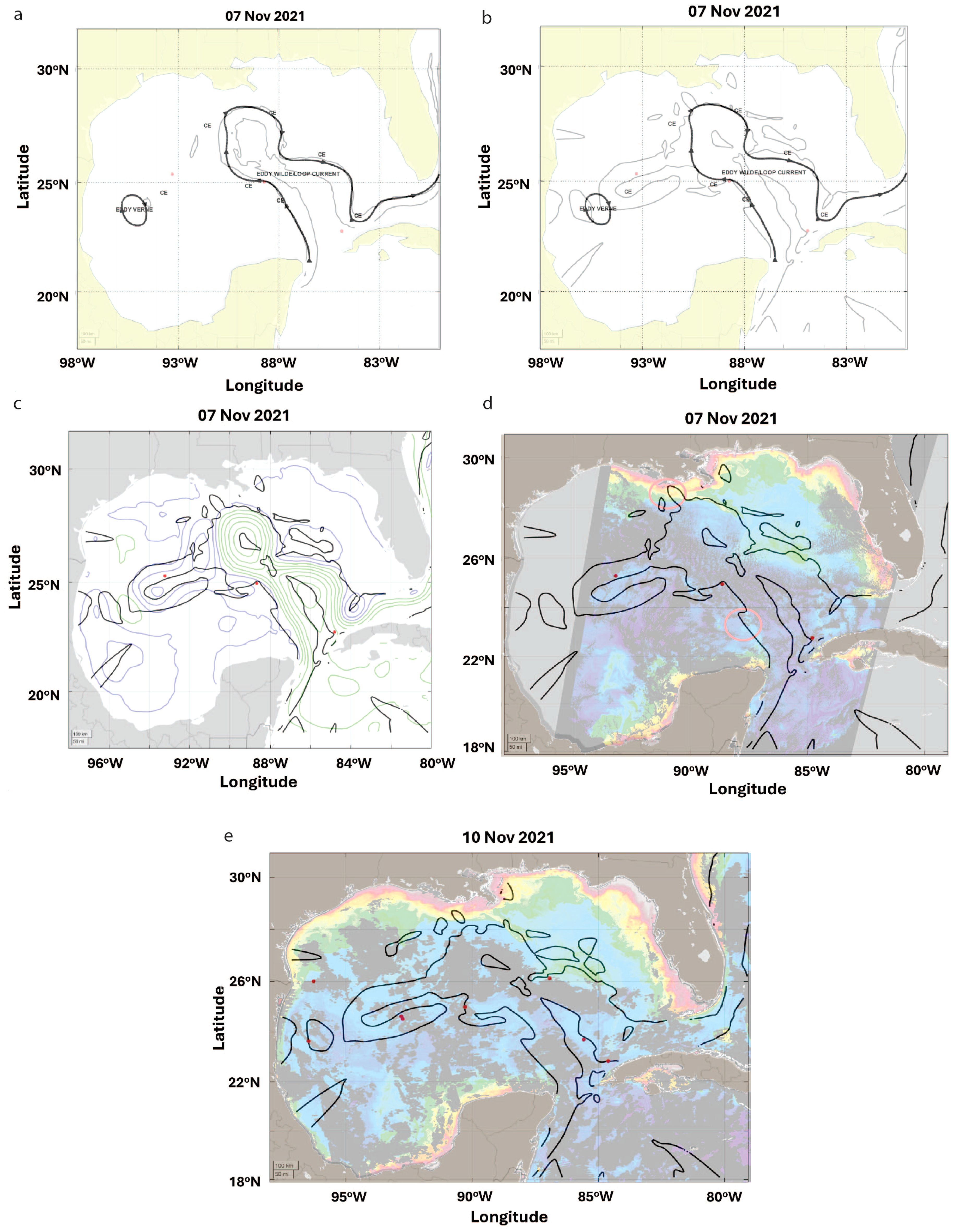
Figure 13. The 0.7 m.s⁻¹ velocity contours from the PINN-SR reconstructed field are compared to the circulation features in the data assimilated (DA) numerical model, EddyWatch^® and the satellite MODIS chlorophyll-a (Chl-a) obtained from the Optical Oceanography Observatory at University of South Florida. (a) 0.7m.s⁻¹ velocity contours from DA model (grey line) and from EddyWatch^® (thick black line with arrows) on 07 November 2021. CE stands for cyclonic eddy and the red dots show the position of the drifters whose velocity was equal to 0.7m.s⁻¹ on that day. (b) 0.7m.s⁻¹ velocity contours from the PINN-SR reconstructed velocity field (grey line) and from EddyWatch^® (thick black line with arrows) on 07 November 2021. (c) DA model SSH contours (colored) overlaid on PINN-SR reconstructed velocity field contours (black line). Positive (negative) heights are shown in green (blue). (d) MODIS satellite chlorophyll-a image on 07 November 2021 overlaid with PINN-SR reconstructed velocity field contours. Colors show the Chl-a concentration and the red circles indicate the presence of circulation features in the Chl-a captured by the velocity contours. (e) Same as (d) on 10 November 2021.

The agreement between the chlorophyll field features and the reconstructed circulation is further shown on 10 November 2021, where a greater number of drifters are present along the contours and where small-scale circulation features that are present in the chlorophyll-a image are also captured by the reconstructed velocity. Note that the velocity contours are likely to not reveal the closed contours of every feature because of the asymmetries in the strain rates and circulation that result in strong deformations of the flow features (Zhang et al., 2024b). Thus, the velocity contours will include frontal features that exhibit the same velocity.

This property would explain to some degree the presence of velocity contours that are offset from the circulation features in the vicinity of Eddy Verne as the eddy speed fluctuates. However, the number of drifters present is that region over the three-month period could have been insufficient to properly capture the eddy velocities, although features situated near the eddy could exhibit higher or equal velocities, which the drifter position, on 10 November, west of the Eddy Verne suggests (Figure 13e). In the LC region, the MODIS image reveals the presence of a multitude of small-scale circulation features that are present along the LC front, north of the LC, some of which appear in the isotach field.

4 Conclusion

Traditionally, surface velocity fields are obtained from altimetric data by geostrophy, which implies that only the geostrophic component of the horizontal velocity field is captured (Wunsch and Stammer, 1998). The increasing interest and need for estimating surface advective transport at 10–100-km spatial scales over relatively short, days to weeks, time scales strengthens the need for velocity observation that resolves submesoscale and mesoscale dynamics (Berta et al., 2015). In contrast to satellite-based altimetry, surface drifter observations provide direct estimates of the local surface velocity field. Although drifter information is routinely used to infer statistical information on basin-scale velocity (Ohlmann et al., 2001; LaCasce, 2008), inferring the velocity field surrounding the drifters has remained challenging due to the sparsity of its observations.

In this study, we assessed the feasibility of reconstructing the velocity field in a large area with a relatively small number of drifters using a deep learning approach. Although we could have used drifters from the various Lagrangian experiments cited in this study, we would have been limited by the lack of validation data, namely the observed velocity field surrounding the drifters. To remedy this challenge, we decided to simulate virtual trajectories with a DA model and use the Eulerian velocity field as the reference. Our approach is rooted in the application of the PINN method, which has been applied in various fields of flow dynamics, from hemodynamics to photonics.

To assess the PINN-SR performance using virtual drifters, we compared the reconstructed field generated by the MLP (no physics learning) and commonly used interpolation methods such as IDW and Kriging. We used relevant metrics such as the RMSE, which quantifies the difference between the prediction and a reference field; the CC, which quantifies how similar two signal variations are; and the MS-SSIM, which is best suited to assess the 2D structural similarity between two images at a patch level and multiple scales. The PINN-SR method performed, as expected, significantly better than the other three methods and showed reduced sensitivity to the evolution of the velocity field (Figure 7). Figures 8, 9 illustrate how the lack of physical dynamics learning through PDEs affects the reconstruction of the velocity field by MLP, IDW and kriging, although the location of the dominant features is accurately located in the MLP reconstructed field. We also evaluated the PINN-SR model with real drifters data, which showed the alignment of the reconstructed velocity contours with the SSH contours of the DA model, rather than its velocity contours, and the correct estimation of the velocity magnitude. In addition to the main circulation features being resolved by the reconstructed field, Chl-a satellite imagery also confirmed the resolution of small-scale energetic features, further validating the reconstructed velocity field.

Due to the limiting role of the sparsity of drifter data, we also examined the effect of the number of drifters on the reconstructed field using the PINN-SR method. Using all three metrics, we showed that the model skill tends to plateau for a number of drifters greater than 250, equivalent to 1.9342 drifters per sq. degrees. Although this number is specific to the GoM region and is associated with a random seeding of the drifters, our study shows that it is sufficient to properly capture the daily LC dynamics on a monthly basis. However, we have not demonstrated that we can reconstruct the velocity field of the complete evolution of the LC, which will be the focus of a future study. The effect of the spatial distribution of the drifters’ initial position is likely to influence the reconstructed velocity field. In a future study, we will address how deployment locations affect the reconstructed field and identify an efficient sampling strategy that minimizes the number of drifters required to properly reconstruct the velocity field at a given location. Indeed, the number of drifters needed and the collocation points for a full velocity field reconstruction impose limitations on the measurement and computational costs.

Despite its nonlinear function representation capability, an MLP could not capture the features of the velocity field as efficiently as the PINN-SR did. It highlights the strength of the PINN method, which, by design, learns the underlying physical processes, greatly improving the reconstruction of flow dynamics through learning of the governing PDEs, hence the flow reconstruction as shown in Figures 8, 9. The physics learning component was shown to be essential for the capture of the circulation features dynamics by the PDEs, which improved the resolution of the mesoscale dynamics. The SR component maintains the efficacy of the method by reconstituting the PDEs with as few coefficients as possible. Although the PDEs are not explicitly provided, they directly contribute to the reconstruction of the velocity field, as demonstrated in our experiments. As far as we know, this is the first attempt to reconstruct the sea surface velocity field with a deep learning model trained only on drifters’ data.

Another aspect to consider is the computational cost of the PINN-SR: training takes roughly 6 h 15 min, whereas each inference completes in just a few milliseconds. Despite this higher upfront expense compared with classical interpolators, the negligible run-time and significantly better accuracy make the network well suited for rapid spatial field reconstruction beyond the drifter locations used for training.

Finally, estimating the Eulerian velocity field from Lagrangrian drifter velocity for data assimilation remains a challenge in oceanography. The velocity of the drifters depends on the influence of various forces, including downwind slippage, Stokes drift, actual surface current, and vertical shear, which is also the result of several constituents. Changes in geometry due to drogue loss, biofouling, and design modification can also lead to a significant variation in observed velocity relative to water speed (Lee and Maximenko, 2025). Wind/wave effects can be identified using a combination of geostrophic velocity from altimetry and wind stress (Lumpkin et al., 2013). However, an important implication of the PINN model not addressed in this study would be the estimation of the contributions of each of the above components through the calculation of the loss function as done in Schmidt et al. (2024) and Limousin et al. (2025) to estimate the separate effects of physical constraints. This approach would greatly enhance the assimilation benefits of drifter velocities by selecting the component to be assimilated. As shown by the extensive literature on the application of PINN to resolve any flow dynamics in various fields and Reynolds flow regime, there appear to have less and less limitations with respect to the resolution of complex flows, including highly variables flow such as tidal currents (Zhang et al., 2024a).

Data availability statement

All the data used in this study can be found here (Bang et al., 2024) and the code here https://github.com/chironbang/PinnDrifters.

Author contributions

CB: Formal analysis, Methodology, Software, Writing – original draft, Writing – review & editing. ASA: Writing – review & editing. HZ: Methodology, Supervision, Validation, Writing – review & editing. AA: Writing – review & editing. AS: Writing – review & editing. LC: Conceptualization, Methodology, Supervision, Writing – review & editing.

Funding

The author(s) declare financial support was received for the research and/or publication of this article. This research was supported in part by the U.S. Department of Energy (DOE) under grant number DE-EE0011382.

Acknowledgments

The authors would like to thank the Woods Hole Group for providing the EddyWatch^® drifter data and velocity contours for this study.

Conflict of interest

Author AS was employed by the company Tendral, LLC.

The remaining authors declare that the research was conducted in the absence of any commercial or financial relationships that could be construed as a potential conflict of interest.

The author(s) declared that they were an editorial board member of Frontiers, at the time of submission. This had no impact on the peer review process and the final decision.

Generative AI statement

The author(s) declare that no Generative AI was used in the creation of this manuscript.

Any alternative text (alt text) provided alongside figures in this article has been generated by Frontiers with the support of artificial intelligence and reasonable efforts have been made to ensure accuracy, including review by the authors wherever possible. If you identify any issues, please contact us.

Publisher’s note

All claims expressed in this article are solely those of the authors and do not necessarily represent those of their affiliated organizations, or those of the publisher, the editors and the reviewers. Any product that may be evaluated in this article, or claim that may be made by its manufacturer, is not guaranteed or endorsed by the publisher.

Footnotes

^ ∥.∥₀ represents the L₀ norm, also called zero norm and ∥.∥₁ the L1 norm also called Manhattan distance
^ Collocation points are the (randomly or adaptively) sampled space-time coordinates where the PINN evaluates the PDE residual, forcing the network to satisfy the physics at those points. They are sampled across the entire prescribed space-time domain.

References

Bang C., Altaher A. S., Zhuang H., Altaher A., Srinivasan A., and Chérubin L. M. (2024). Data assimilated numerical model velocity data. doi: 10.5281/zenodo.10968693