 Dian Zhang1
 Weiwei Yu2*
 Bin Chen2Huamei Huang3
 Jianji Liao2Lingyang Feng2
 Guangcheng Chen2
 Zhiyuan Ma2Qinhua Fang1*
 Shunyang Chen2
 Bin Xie2Zhiyi Kan1Shangke Su2
 Ge Feiyang4Hanmeng Yuan5
- 1College of the Environment and Ecology, Xiamen University, Xiamen, Fujian, China
- 2Third Institute of Oceanography, State Oceanic Administration, Xiamen, China
- 3South China Sea Institute of Planning and Environmental Research, Ministry of Natural Resources, Guangzhou, China
- 4South China Sea Ecological Center, Ministry of Natural Resources, Guangzhou, China
- 5Shenzhen Urban Planning and Land Resource Research Center, Shenzhen, China
Introduction: Understanding ecosystem degradation and estimating its extent are essential to enact decision-making policies in biodiversity conservation, ecosystem restoration, and management. Although many approaches have been proposed to identify the degradation status of an ecosystem, the heavy data burden required lacks targeted degradation information to inform such decision-making restoration policies.
Methods: This study proposes a multi-tiered decision-making framework to diagnose ecosystem degradation based on the most common restoration models that link degradation to restoration. The degradation diagnosis process can be executed step-by-step (i.e., in a physical to chemical to biological order). This study selected a limited number of coastal bay indicators from each layer, and a conceptual ecosystem response profile was applied to guide their degradation criteria settings: stepped for physical indicators, hump-shaped for chemical indicators, and smooth for biological indicators. Daya Bay in China was selected for this case study.
Results: In total, 62% of the bay has degraded by varying degrees, including completely degraded, heavily degraded, moderately degraded, and slightly degraded percentages were 4.64%, 3.78%, 15.16%, and 38.43%, respectively. Moreover, there has been a gradual but continuous spatial change in its degradation degree from north to south and from west to east.
Discussion: Results from this study can be used to identify and prioritize restoration processes. Human-assisted restoration efforts should prioritize its moderately degraded western section and its heavily degraded coastal areas along Yaling Bay and Fanhe Harbour. Our framework provides an efficient, science-based, and novel approach to diagnose the degradation status of the coast, particularly in the absence of long-term observational data, which can be effectively applied to any region or ecosystem.
1 Introduction
Ecosystem degradation is widely defined as an adverse change in composition, structure, functionality, or even goods and services, subsequently becoming a global issue of concern (Delgado and Marín, 2020). Ecosystem restoration is a crucial approach used to reverse and restore ecosystem degradation (Saunders et al., 2020). Understanding ecosystem degradation and estimating its extent is of utmost importance for restoration decision-making policies (McDonald et al., 2016; Saunders et al., 2020). Numerous international policies support ecosystem restoration, such as United Nations Sustainable Development Goals, United Nations Decade of Ecosystem Restoration (2021–2030), Post-2020 Global Biodiversity Framework, and Decade of Ocean Science for Sustainable Development 2021–2030. Various frameworks have been established to address global ecosystem degradation, each with unique focuses. However, current frameworks exhibit significant limitations in bridging ecosystem degradation diagnosis with restoration strategies, which constrains the effectiveness of management practices. For instance, the IUCN Red List of Ecosystems (RLE) identifies the risks of ecosystem collapse but lacks restoration strategies (Bland et al., 2017). The Ocean Health Index (OHI) evaluates the sustainability of marine environments, emphasizing ecosystem services (Halpern et al., 2012). While these frameworks provide valuable insights and tools for comprehending ecosystem conditions, they mainly describe current state rather than offering methods to assess degradation or explicit restoration strategies. Crucially, the fundamental purpose of ecosystem degradation assessment is to inform restoration strategies, distinguishing it from mere health evaluations or risk classifications. The SER International Standards for Ecological Restoration address various facets of ecosystem recovery (SER, 2002; McDonald et al., 2016). There is an urgent need for a model that can diagnose ecosystem degradation diagnosis model to inform and guide restoration efforts.
Ecosystems are inherently dynamic. They involve complex interactions while being exposed to various disturbances, which can often cause irreversible changes (Martina et al., 2020). This complexity makes it challenging to assess their degradation status (Yando et al., 2021). A variety of approaches have been proposed to evaluate degradation, such as ecosystem indicators against reference values or thresholds, particularly focusing on biological diversity, composition structure (Yuan et al., 2014; Sasaki et al., 2015), and ecosystem services reduction (Sutton et al., 2016; Sharafatmandrad and Khosravi Mashizi, 2021). Other approaches use anthropogenic pressures to infer degradation (Cotroneo et al., 2018; Holon et al., 2018) and develop comprehensive indices that combine multiple indicators (Zhu et al., 2011; Yuan et al., 2014; Lin et al., 2021). Despite these approaches, numerous challenges persist, particularly regarding data scarcity. Many assessment techniques require extensive data (Thompson et al., 2013), which is often unavailable, particularly for coastal and marine ecosystems, due to their inherent complexity and high cost of oceanic investigations (Henriques et al., 2014). Besides, the use of too many indices can complicate understanding degradation pathways of degradation (Bland et al., 2017), and degradation findings in many studies are often insufficient to inform restoration decision-making policies (Davidson and Finlayson, 2019; Zhou et al., 2017). To address these issues, there is an urgent need for a streamlined, theoretically robust decision-making framework that directly links degradation assessment with restoration strategies, providing clear direction for ecosystem management and recovery.
Ecosystem degradation may result in regime shifts, where crossing a threshold or tipping point leads to a transition to a different state (Horan et al., 2011). These thresholds or tipping points inform the ecosystem state, indicates when and how much effort is needed for restoration (Jamsranjav et al., 2018). Restoration strategies should ideally be tailored ecosystems’ degradation states. Numerous restoration theories and models explain the relationship between degradation and restoration (King and Hobbs, 2006), Among these, with Milton’s et al. (1994) being most influential (Hobbs and Norton, 1996; Suding and Hobbs, 2009; McDonald et al., 2016; Aronson et al., 2017). The essential factor of this classic model is its threshold theory, which states that the transition between alternative stable states may occur when an ecosystem crosses a critical threshold (Bestelmeyer, 2006; Majumder et al., 2019). This conceptual model assumes that two thresholds represent barriers to potential ecosystem recovery: a biotic barrier and an abiotic barrier, which inform the three main degradation stages of these two barriers (McDonald et al., 2016). Degradation and restoration are regarded as continuous processes punctuated by stepwise changes at thresholds are crossed (King and Hobbs, 2006). Understanding these crucial factors and their potential thresholds that are used to determine ecosystem status will provide novel insight into diagnosing the degradation status and associated linkages that guide restoration initiatives. However, such theoretical models have rarely been applied in quantifying and identifying degradation to inform targeted restoration strategies, particularly with respect to complex coastal and marine ecosystems.
A coastal bay is a body of water enclosed by land on three sides. Coastal bays are one of the most biologically diverse and productive ecosystems on Earth (Castagno et al., 2018). However, they are continuously subjected to ecosystem degradation, predominately caused by anthropogenic activities (Li et al., 2021). Accordingly, coastal bay restoration has received more and more attention in recent years (Zhou et al., 2020). In this study, using a coastal bay in China as a case study, we developed an integrated degradation assessment approach i) to propose a multi-tiered conceptual framework to assess degradation based on a theoretical degradation and restoration model and ii) to identify suitable indicators and associated thresholds for each diagnostic tier. At the same time, this approach was applied to assess the degradation of Daya Bay in the northern section of the South China Sea. This will enrich the data pool to enhance Daya Bay coastal bay ecosystem management, which involves its degradation status, critical degradation factors, restoration approach, priority area, etc. Finally, this study aims to enhance restoration-oriented decision-making policies specific to degradation diagnostic approaches while providing a framework that can be built upon and modified for use in other ecosystems.
2 Methods and data
2.1 Methods
2.1.1 Conceptual model
The diagnosis of ecosystem degradation involves a methodological framework that translate natural scientific data to management information for decision makers. The essential step is the development of a science-based conceptual model. Theoretically, ecosystem components respond differently to external changes, which can be complex, reversible, or irreversible. Each stage of degradation involves various factor, including physical, chemical, and biological processes. Coastal bays have strong interactions between abiotic and biotic elements, with the abiotic environment being crucial for all organisms, particularly those in the physical environment, corresponding to the basic structure of an organism’s ecological niche. Using the classic conceptual framework (i.e., the two-barrier model) as a basis (Hobbs and Harris, 2001; Suding and Hobbs, 2009), this study hypothesizes three potential underlying states with differing characteristics based on two ecosystem recovery barriers: i) physical habitats that have been completely altered or destroyed; ii) physical habitats that remain intact or are within degradation thresholds, but the chemical environment has exceeded its threshold; iii) the abiotic environment (i.e., both physical and chemical) remained intact or is within degradation thresholds, while biotic elements have been destroyed or beyond their thresholds.
Based hypothesis above, a simplified decision model was developed.to illustrate how the condition of coastal bay ecosystem worsens as they surpass key thresholds in biology, chemistry, and physics (Figure 1). These degradation state were categorized into five levels: non-degraded (ND), slightly degraded (SD), moderately degraded (MD), heavily degraded (HD), and completely destroyed (CD), each with tailored restoration strategies (Figure 1b). Specifically, ND indicates ecosystems in good condition without significant degradation; SD reflects a condition where the biological diagnostic threshold is exceeded but abiotic thresholds (chemical and physical) remain intact; MD represents ecosystems that have crossed the chemical diagnostic threshold but not the physical one; HD and CD indicate that physical thresholds have been surpassed, with CD referring to ecosystems where natural characteristics are almost entirely lost. They highlight the different decisive factors that cause degradation under physical, chemical, and biotic perspectives, even though they interact or occur simultaneously rather than being strictly independent (Figure 1a). Critically, while the model appraises the targeted restoration approaches for each degradation level, it is important to consider lower-level restoration strategies alongside those for higher levels. For instance, if physical habitat is completely destroyed and ecosystem reconstruction is needed, additional lower-level interventions, such as habitat modification and improved management practices, are also necessary. This aligns with the understanding that the more severe the degradation, the more challenging the restoration process becomes.
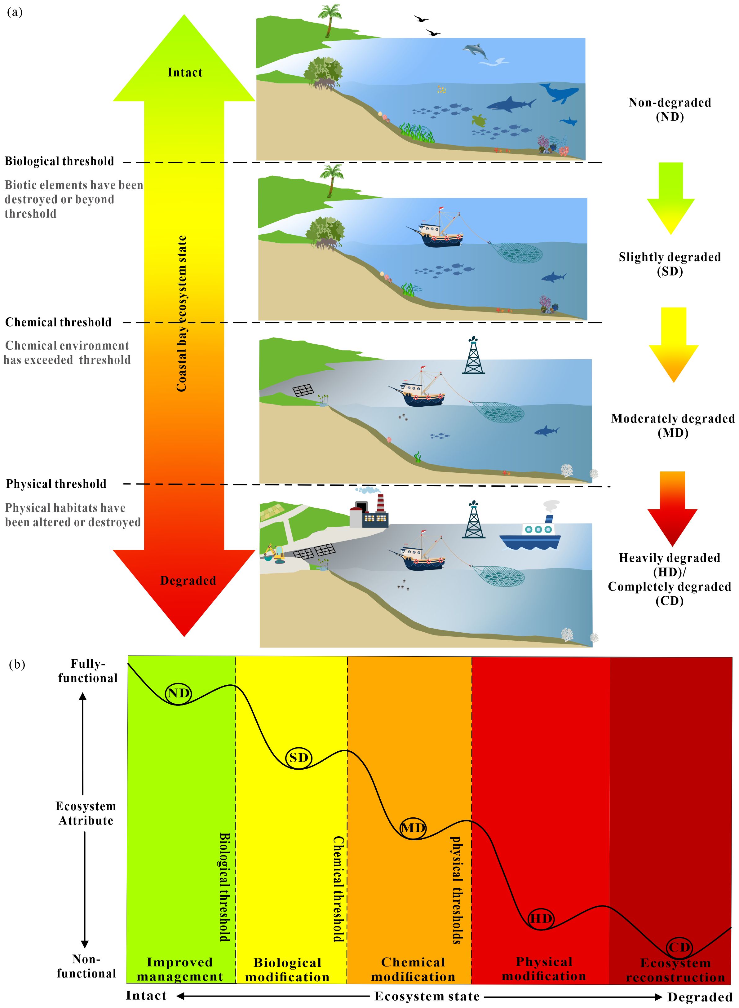
Figure 1. The conceptual coastal bay degradation model. (a) Changes in the coastal bay ecosystem degraded state; (b) The concept model of ecosystem degradation and restoration (modified from McDonald et al., 2016, licensed CC BY-NC 4.0). ND is non-degraded, SD is slightly degraded, MD is moderately degraded, HD is heavily degraded, and CD is completely destroyed.
The model presents a multi-tiered decision-making process structured into three distinct diagnostic stages: physical, chemical, and biological diagnosis (Figure 2). As ecosystem degradation worsens, it becomes easier to distinguish the degraded state from a pristine state due to a more significant constrast with reference data. The model prioritizes abiotic habitat diagnosis, starting with physical diagnosis as the primary decision layer, followed by chemical diagnosis and then biological diagnosis. It aims to minimize initial assessment uncertainties, through prioritizing idenfication of irreversible physical changes. The model assumes that the physical habitat destruction is the most severe form of degradation, inevitably leading to subsequent chemical and biological changes. Artificial habitats are costly and uncertain to restore, whereas semi-natural habitats, like aquaculture ponds are more feasible for coastal wetland restoration (Duncan et al., 2016). Chemical degradation, often linked to human activities, has a higher potential for natural recovery and lower restoration difficulty (Gann et al., 2019). Biological factors show hysteresis in response to environmental changes, making them the final decision layer (Choi et al., 2005; Polo et al., 2022). Thus, there are two critical issues needed to be addressed in this model: identifying diagnosis indicator for each decision node and setting the corresponding thresholds.
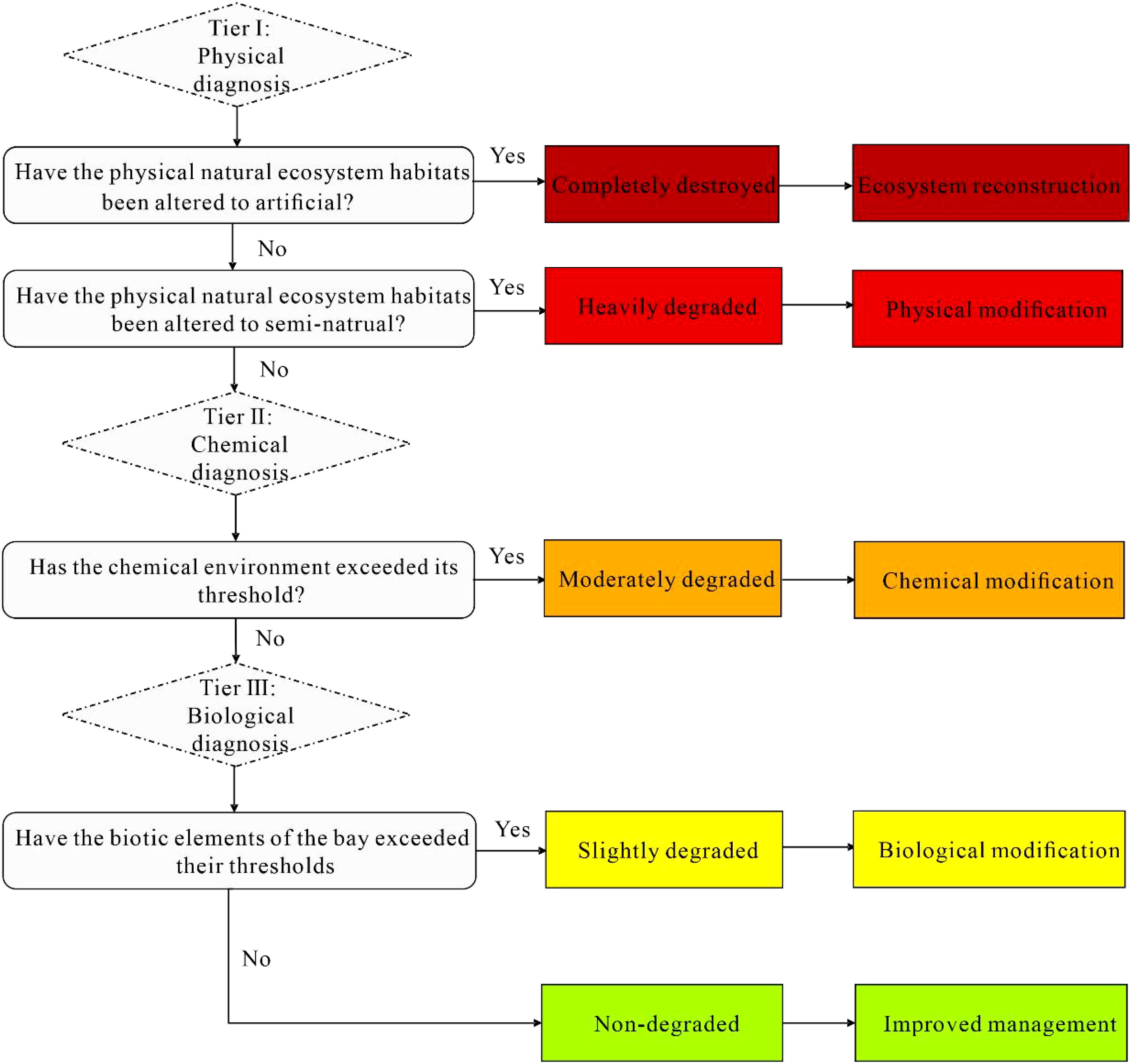
Figure 2. Decision flowchart for degradation diagnosis.
2.1.2 Diagnosis indicators
Many indicators have been used to evaluate the degree of marine ecosystem degradation, such as land cover change (LULC) (Zhou et al., 2017), species biomass loss (Holon et al., 2018), oceanic pollution loads increase, and biodiversity decline (Jiang et al., 2015; Zhou et al., 2017). However, selecting a few effective indicators is essential to avoid oversimplification or confusion (Burgass et al., 2017).
Physical diagnosis focuses on habitat change like landform and substrate type changes. Globally, including along China’s coas, reclamation has been the leading cause for these change (Yuan and Chang, 2021), significantly altering the natural properties of coastal areas. For example, converting a natural coastal wetland to an aquaculture pond shifts its “naturalness” to “semi-naturalness”. Thus, this study uses habitat “naturalness” as a qualitative indicator to rapidly diagnose the degradation level of physical habitat. This is represented by three potential scenarios, namely, natural habitat change will engender a natural, semi-natural, or artificial habitat.
Chemical diagnosis evaluates environmental quality change, particularly in seawater and benthic sediment. To effectively reflect degradation, we focused on key indicators that closely correlate to the habitat requirements and pollution levels, also considering factors like their ease of measurement, cost-effectiveness, and simplicity (Dudley et al., 2018). Dissolved oxygen (DO) is crucial for aquatic life (Guo et al., 2022). Nutrient indicators (i.e., inorganic nitrogen and active phosphate) are typically included due to their prevalence in seawater eutrophication (Andersen et al., 2014). Land-based heavy metals (i.e., Cr, Mn, Zn, etc.) accumulate in sediments, affecting benthic environments and the health of marine organisms (Liang et al., 2023). Environmental indicators should be tailored to the ecosystem’s specific conditions.
Biological diagnosis identifies changes in biological community, including productivity and biological complexity. Coastal bay productivity involves primary productivity (e.g., coastal wetland flora and seawater algae taxon) and fauna production like fish yields. The former can be used as indicators to estimate chlorophyll content in seawater based on resident phytoplankton while the latter can be represented by fish yields, benthic biomass, etc. Biological complexity refers to the variation in the biological structure, process, function, etc., which is generally estimated by biodiversity indicators, such as species diversity (i.e., indicator species) (Duelli and Obrist, 2003) and community diversity (i.e., nekton diversity, benthos diversity, etc.). Healthier ecosystems tend to be regulated more by biotic interactions, whereas for ecosystems with low biotic resources, such resource loss reduces interactive intensity.
Table 1 shows the three diagnosis tiers and their corresponding recommended indicators. Most data necessary for these indicators can easily be obtained by traditional investigation methods or remote sensing.
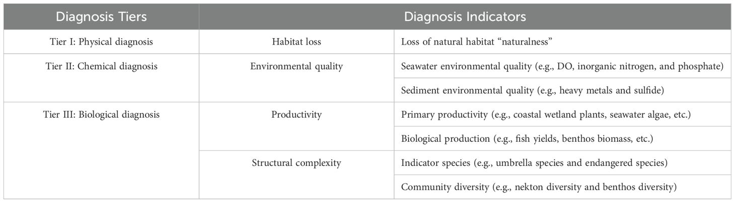
Table 1. Degradation diagnosis tiers and recommended indicators of coastal bay ecosystems.
2.1.3 Degradation thresholds
A threshold is the point or range at which an ecosystem shifts to a different state, and determining these critical thresholds is challenging. Degradation diagnosis is typically regarded as a relative assessment against a healthy, intact or undisturbed ecosystem, with the degree of degradation indicated by the extent of deviation from this reference condition. Defining a baseline reference state is crucial, ideally based on the ecosystem’s pre-degradation state (Kotiaho et al., 2016). On this account, historical data can serve as a reference baseline for an intact or natural state to infer diagnosis thresholds. There are four archetypal ecosystem collapse profile trajectories: abrupt, smooth, stepped, and fluctuating. These profiles illustrate potential ecosystem responses to stress (Bergstrom et al., 2021), offering a theoretical foundation for determining thresholds.
For physical diagnosis, we selected the loss of a natural habitat’s “naturalness” as an indicator, which means a habitat change from natural habitat to semi-natural, or artificial habitat. Ecosystem response to this change tends to be abrupt at each state while appearing stepped when considering all scenarios: і) no change in natural physical habitat; ii) partial loss as habitats shift from natural to semi-natura; ii) compelte loss as habitats become artificial (Figure 3a). Since restoring artificial physical habitats challenging and costly (Stewart-Sinclair et al., 2020), we considered them as a lower threshold and diagnosed as completely destroyed (Figure 2). Correspondingly, semi-natural physical habitats, seen as an upper threshold are diagnosed as heavily degraded, being typically considered high potential restoration targets (Duncan et al., 2016), like aquaculture ponds, cropland, and salterns.
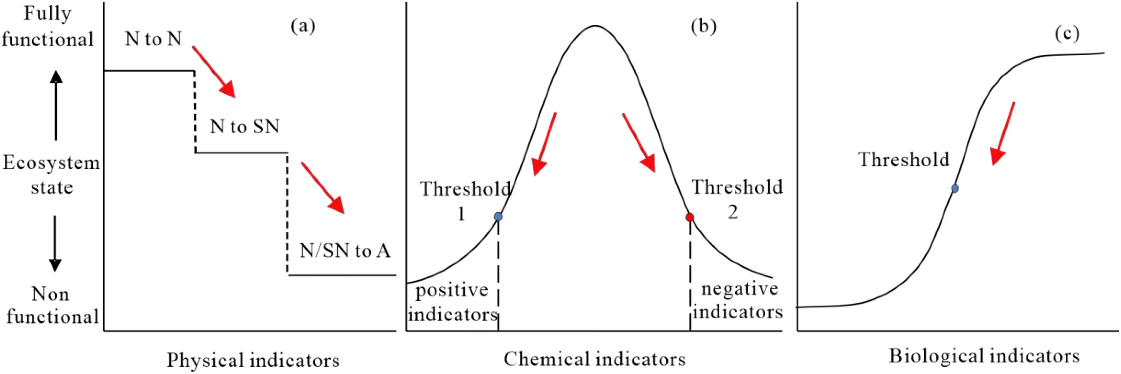
Figure 3. Conceptual framework of ecosystem response to influencing factors. (a) Physical diagnosis (N, natural physical habitats; SN, semi-natural physical habitats; A, artificial physical habitats); (b) chemical diagnosis; (c) biological diagnosis. The red arrow represents the direction of degradation.
For chemical diagnosis, we used environmental quality indicators to gauge chemical environment degradation. Ecosystem response to chemical factors are often exhibiting a hump-shaped pattern (Guimarais et al., 2021). Gaussian mixture models have generally been used to describe these relationships between organnisms and the environment (Cui et al., 2008; Baek et al., 2014), representing ecosystem responses to environmental parameter. Typically, a threshold or a range with two thresholds is used to distinguish between suitable and degraded states (Figure 2b). Environmental quality standards often set the minimum expectation threshold, which serve as the upper threshold for positive indicators (e.g., DO) and the lower threshold for negative indicators (e.g., inorganic nitrogen) (Guimarais et al., 2021; Gibson, 2000). For positive indicators, thresholds are set to 25% of the baseline reference; for negative indicators, thresholds are set to 75% of the baseline reference (Gibson, 2000). This approach has been widely adopted in ecological assessments and provides a statistically robust basis for identifying significant deviations from historical conditions (Yu et al., 2022). Since multiple environmental parameters are often selected, parameters within the same tier are treated as parallel indicators. Diagnostic decisions are then guided by Liebig’s law of the minimum.
For biological diagnosis, many studies have shown that the relationship between biodiversity and ecological processes or functions follows by a logarithmic curve, with a smooth response, and a saturation point as the ecological threshold (Tilman et al., 1997b, 1997). It hypothesized that the response follows a decreasing trend with a distinct threshold or tipping point (Figure 3c). Many studies have conducted long-term monitoring and quantification regarding the definition of biotic thresholds (Kelly et al., 2015; Toth et al., 2015; He et al., 2021). A typical example is vegetation cover (i.e., from approx. 10%–30%) as a biotic threshold (Gao et al., 2011). Defining universal thresholds for each indicator is tough, especially for complex coastal bay ecosystems. Here, the biotic threshold was set to the minimum value of multiple baseline references, with the ecosystem considered slightly degraded when below this value (Figure 3c). This conservative approach helps reduce uncertainty associated with biological variability and avoids overestimating degradation.
2.2 Study area
Daya Bay is one of the largest semi-enclosed bays along the South China Sea’s northern coast, situated on the eastern side of the Pearl River Estuary. It is surrounded by the Dapeng Bay in Shenzhen to the southwest, the Huiyang District to the northwest, and Huidong County in eastern Huizhou, which serves as an important center for ports and shipping, the petrochemical industry, the nuclear power industry, and mariculture and tourism in the Pearl River Delta. Daya Bay habitat types are diverse (i.e., mudflats, mangroves, rock reefs, and coral reefs). The bay is rich in biodiversity and is home to a variety of marine organisms, which include threatened species such as the black-faced spoonbill (Platalea minor) and the green sea turtle (Chelonia mydas).
Daya Bay’s large-scale and intensive development mainly began after China enacted its Economic Reform and Opening-Up policies (Qu et al., 2018). Prior to this period (1980S), the bay ecosystem maintained relatively pristine conditions with minimal anthropogenic impacts (Yu et al., 2022). This study therefore regarded the 1980s as the reference degradation period. Thus, the area of the natural bay region in the 1980s (i.e., 841.42 km2) was defined as the boundary of study area, where the landward boundary was determined by the 1982 coastline and where the seaside was bounded by the mouth of the bay (Figure 4a).
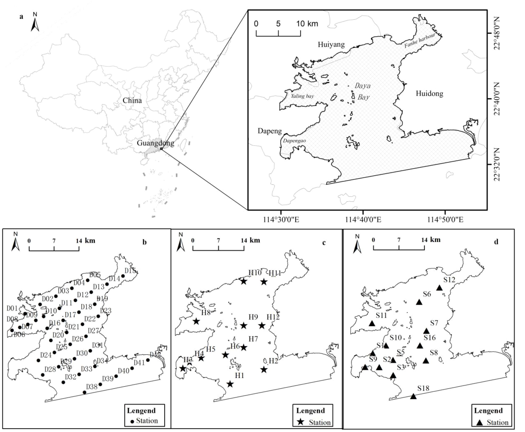
Figure 4. Study Area and distribution of chemical and biological indicators (a: the study area; b: the sampling sites in status quo; c: the sampling sites of long-term survey data for chemical diagnostic indicators; d: the sampling sites in 1987 for biological diagnostic indicators).
Diagnostic indicators for Daya Bay, as shown in Table 2, were selected based on degradation diagnostic tiers and suggested indicators from Table 1. In addition, indicator selection also considered data availability across historical and contemporary periods, as well as the specific ecosystem characteristics of Daya Bay. Following the wetland classification (GB/T24708-2009), land use status classification (GB/T21010-2017), and IPCC land cover types, coastal wetland habitats in this study were classified into natural, semi-natural, and artificial habitats. Natural habitats comprise shallow water, woodland, and mudflats; semi-natural habitats include aquaculture ponds; artificial habitats consist of impervious surfaces. To quantify the degradation of physical habitats loss, we employed ArcGIS spatial analysis tools and the raster calculator to detect habitat type transitions between historical and current periods, and to calculate the associated area loss.
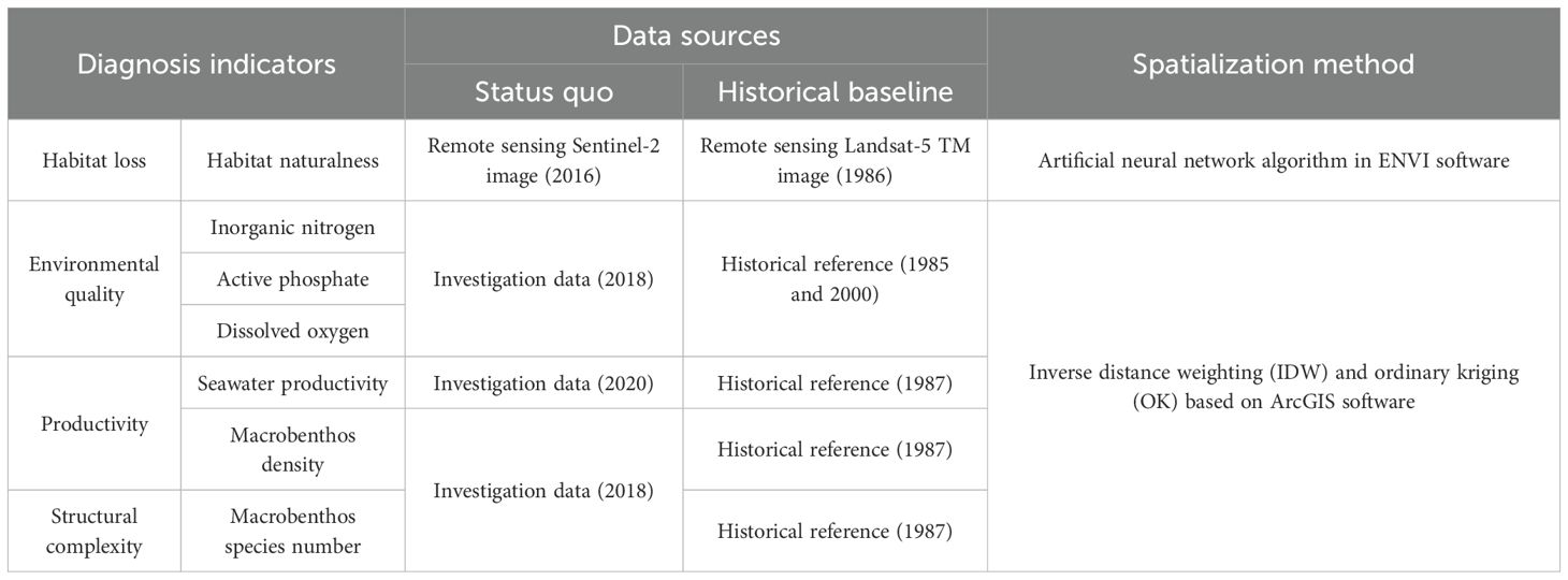
Table 2. Diagnosis indicators, data sources, and spatialization methods for Daya Bay’s ecosystem degradation.
Chemical and biological diagnostic indicator data were obtained from investigations conducted at 76 sampling sites in 2018 and 2020 (Figure 4b), covering primary productivity (37 sampling sites), benthos (39 sampling sites), and seawater environments (39 sampling sites). Historical references were obtained from 11 long-term survey data for chemical diagnostic indicators (Figure 4c) and 12 sampling sites in 1987 for biological diagnostic indicators (Figure 4d). To provide a more accurate and spatially defined degradation diagnosis reference, all data were correspondingly interpolated to 30×30 m using the interpolation method of IDW and OK (Supplementary Figures S1, 2). Spatial autocorrelation test and accuracy assessment were shown in Supplementary Table S1 and Supplementary Figure S3 of Supplementary Materials.
Quantile-percentile methods were applied to infer thresholds for chemical diagnosis indicators (Gibson, 2000), where long-term chemical indicator data (1985-2000) were used as reference baselines, whose data sources were compiled from field surveys conducted by the National Institute of South China Sea Studies. Biological diagnostic indicator thresholds were set to the minimum value of the baseline reference observed in the 1980s (Tilman et al., 1997a), where it was assumed that even meeting the minimum state of an intact ecosystem constituted a healthy environment.
The step-by-step degradation diagnosis was conducted according to the decision flow (shown in Figure 2) to determine the degradation level and inform its corresponding restoration strategies.
3 Results
3.1 Tier I diagnostic results
Daya Bay’s physical habitats significantly changed between 1986 and 2016 (Figure 6). In 1986, its natural, semi-natural, and artificial habitat areas were 814.54 km2, 10.34 km2, and 8.72 km2, respectively. The bay’s total natural habitat area (64.57 km2) was subsequently transformed to semi-natural habitats (25.71 km2) and artificial habitats (38.86 km2), diagnosed as being “completely destroyed” and “heavily degraded”, respectively. The tidal flat loss rate was highest (98.63%) among all habitats (Table 3). Spatially, completely degraded areas were mainly distributed in Daya Bay’s northwestern waters while heavily degraded areas were mainly distributed in the inner bay and ports along the coastlines of Yaling Bay, Fanhe Harbour, and Dapeng Bay (Figure 5a).
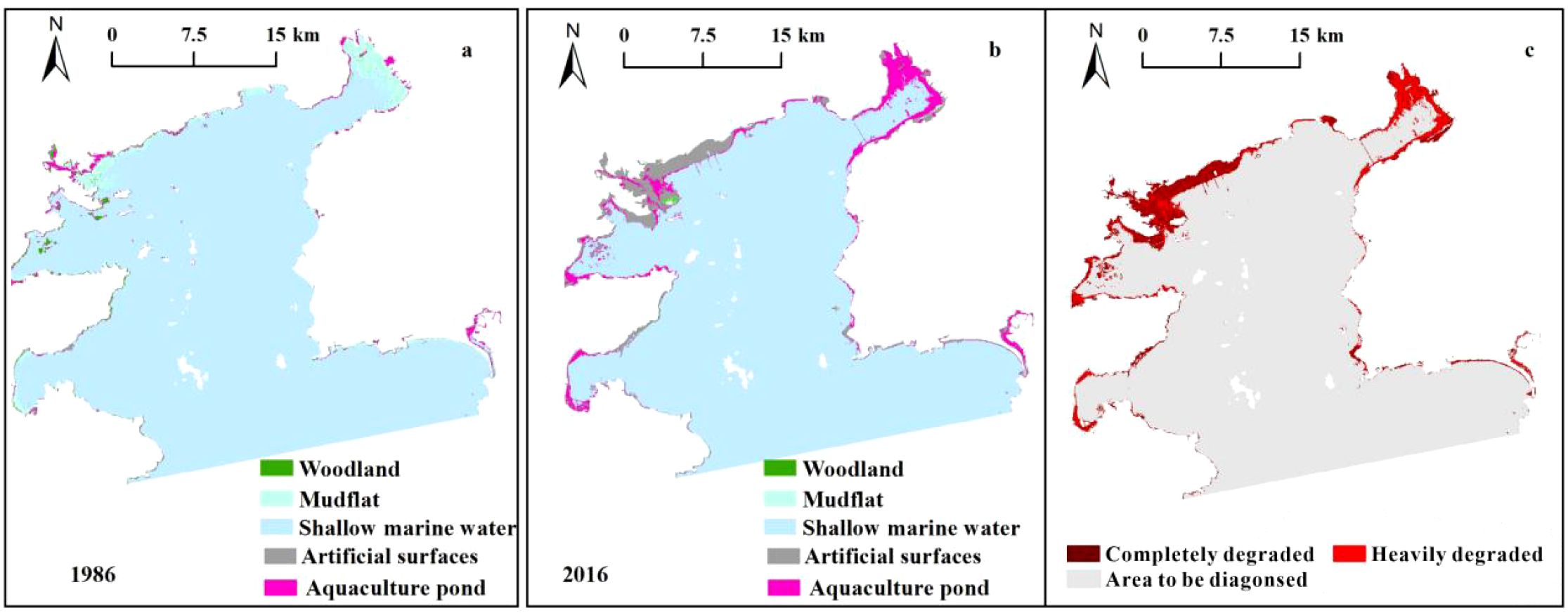
Figure 5. Spatial results of physical diagnosis (c) and habitat type distribution in Daya Bay in 1986 (a) and 2016 (b).
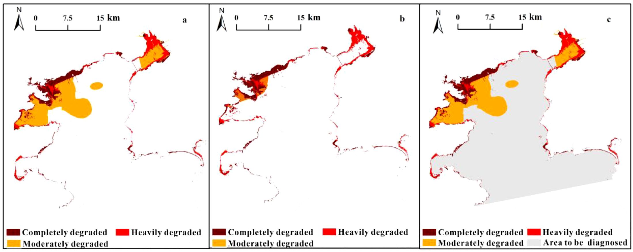
Figure 6. Spatial chemical diagnostic indicator results from Daya Bay (a: inorganic nitrogen; b: active phosphate; c: chemical diagnosis).
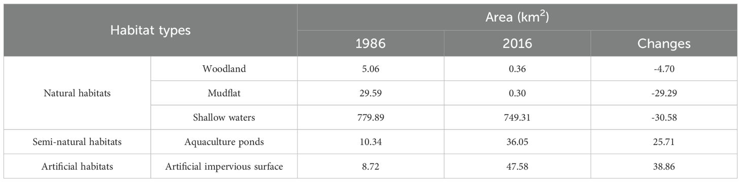
Table 3. Habitat change area in Daya Bay between 1986–2016.
3.2 Tier II diagnostic results
Based on physical diagnostic results, Tier II chemical diagnosis was conducted in the remaining areas. Table 4 provides the chemical parameter concentration range used for diagnosis indicators. Since DO in 2018 was found be higher than that in the 1980s and did not exceed the thresholds, no signs of degradation were observed for this parameter. The diagnosis of the two parallel indicators (i.e., inorganic nitrogen and active phosphate) indicated that an approximate area of 127.58 km2 was diagnosed as being moderately degraded, among which inorganic nitrogen constituted 127.58 km2 (Figure 6a) while active phosphate constituted 18.92 km2 (Figure 6b), and the degraded areas by these two indicators overlap to a large extent. Moderately degraded areas were mainly distributed in the northwestern waters of Daya Bay and Fahe harbor.
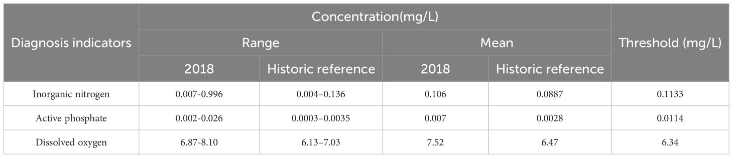
Table 4. Chemical diagnostic indicator concentration ranges.
3.3 Tier III diagnostic results
Tier III biological diagnosis was conducted in the remaining areas after Tier I and Tier II diagnosis concluded. Table 5 provides biological indicator values. A decreasing trend in seawater productivity was observed from central to coastal and outer waters. High macrobenthos density values were observed in Daya Bay’s central water region and water around the Daya Bay Nuclear Power Station. Additionally, high macrobenthos species number values per station were observed in Yaling Bay and Daya Bay’s southwestern waters. The spatial distribution of macrobenthos species numbers was mostly counter to that of its density. Approximately 323.24 km2 was diagnosed as being slightly degraded based on biological diagnosis thresholds, among which no area was identified based on primary productivity (Figure 7a), 21.14 km2 was diagnosed by macrobenthos density (Figure 7b), and 323.24 km2 was diagnosed by macrobenthos species number (Figure 7c). Slightly degraded areas were showed a tendency of spreading from the inner bay to the outer bay.
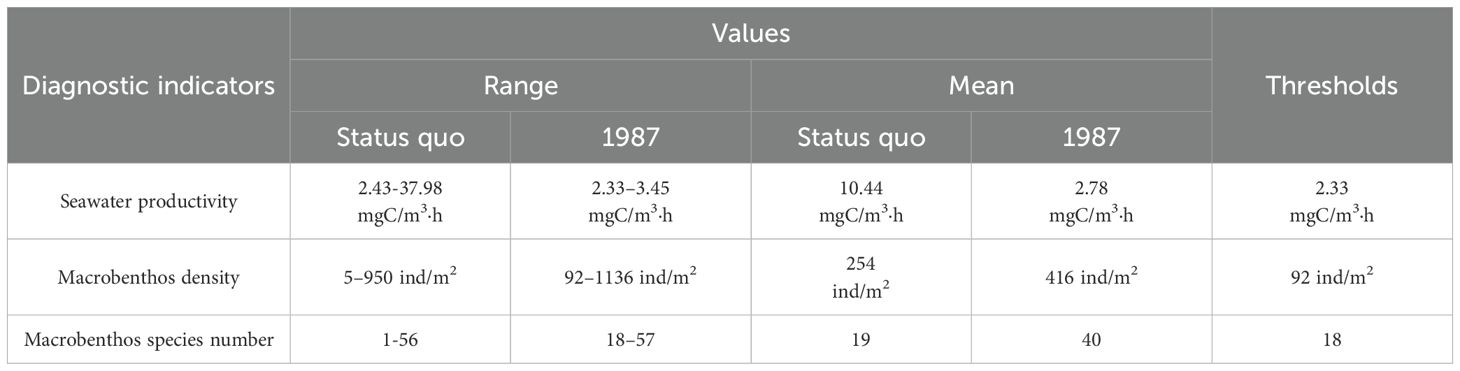
Table 5. Biological diagnostic indicator values.
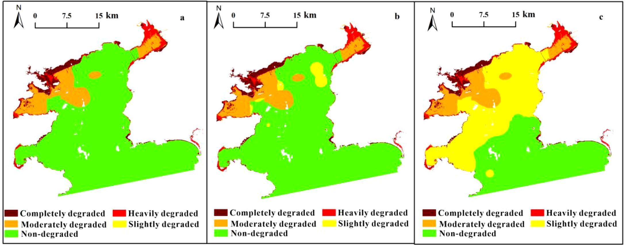
Figure 7. Spatial biological diagnosis indicator results for Daya Bay (a: primary productivity; b: benthos density; c: species number of benthos).
3.4 Final diagnosis decision and restoration summary recommendations
The three tier results showed that Daya Bay’s total degraded area was 527.21 km2, exhibiting varying degradation degrees, which cover 62% of the entire study area. Pertaining to the degradation level, completely degraded, heavily degraded, moderately degraded, and slightly degraded percentages were 4.64%, 3.78%, 15.16%, and 38.43%, respectively (Figure 8). Generally, spatial distribution was characterized by a degradation degree trend from Daya Bay’s northwestern to southeastern waters. Completely degraded areas were mainly distributed in Daya Bay’s northwestern waters, where ecosystem reconstruction is required. Heavily degraded areas were mainly distributed in estuary and port areas along Daya Bay’s coastline (i.e., Yaling Bay and Fanhe Bay), where physical modification is required. Moderately degraded areas were concentrated in Daya Bay’s northwestern waters and Fanhe harbor, where chemical modification is required. Certain slightly degraded areas in the inner bay offshore western section require biomodification (Figure 8).
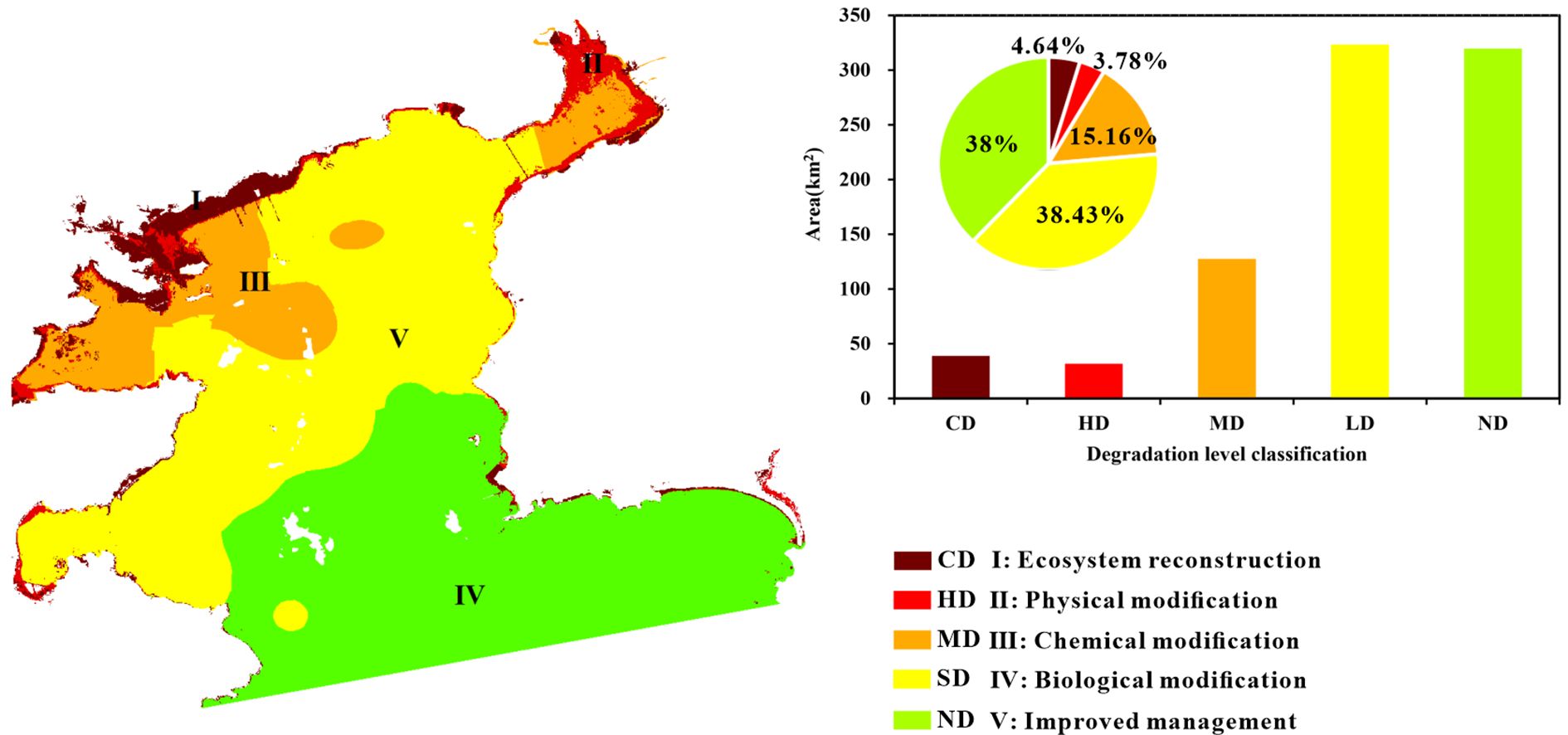
Figure 8. Spatial distribution and area degradation in Daya Bay.
4 Discussion
4.1 Daya Bay restoration priorities
The results revealed spatial heterogeneity in the degradation degrees, with the western waters being more degraded than the eastern ones. This suggests a strong association between anthropogenic activities with the degree of degradation, which is consistent with previous health assessments of Daya Bay (Yu et al., 2022). The degraded areas were predominately found in the western waters of Fanhe Bay and Daya Bay (Figure 8), coinciding with the bay’s main economic center (Man et al., 2022). Huiyang District had the highest urbanization rate and per capita GDP among all counties around the bay, also showed the most severe degradation.
The degree of ecosystem degradation was largely influenced by the factors affected, whether physical, chemical, or biological. Physical habitat destruction, mainly due to large-scale reclamation, was a significant cause of severe and extensive degradation, particularly along the inshore area of Daya Bay (Figure 5). Chemically, there was a significant downward pattern of degradation from northwestern to southeastern (Figure 6), with eutrophication being the primary cause, which is consistent with previous studies (Wang et al., 2004). Interestingly, the near the Daya Bay Nuclear Power Plant had less chemical degradation, possibly due to warm effluents promoting phytoplankton growth, which reduces nutrient concentrations (Peng et al., 2001).
Macrobenthos indicators have significantly contributed to biological diagnosis, with species richness decreasing along most coastal waters of Daya Bay, showing high sensitivity to environmental changes, which is essential for assessing ecosystem degradation (Yokoyama et al., 2007). This aligns with previous findings of a simplified benthic community structure over time (Du et al., 2011; Zhang et al., 2021). The local conservation efforts may have influenced this trend by increasing the abundance of certain species, potentially reducing overall diversity. Slightly degraded areas, identified by macrobenthos, often correlated with moderately degraded areas identified by chemical indicators. Overlay analysis showed in areas identified as chemically degraded, 78.31% also met the biological degradation threshold by macrobenthos. It suggests that some pollution impact on the benthos community. Overfishing may also have influenced macrobenthos composition by altering the food chain (Zhang et al., 2020).
From the perspective degradation status alone, restoration priority in Daya Bay should be given to moderately degraded western areas and heavily degraded areas along the Yaling Bay and Fanhe harbor coastlines. This is because completely destroyed often indicates low cost-effectiveness in restoration efforts, while slightly degraded areas can typically recover naturally through ecosystem resilience. However, it is important to note that identifying priority restoration areas is a multifaceted process. Beyond degradation status, additional factors must be considered, including potential ecosystem services (Strassburg et al., 2020), habitat suitability (Hu et al., 2021), and restoration costs (Stewart-Sinclair et al., 2020).
Our study evaluated Daya Bay’s degradation, but due to data limitations and the dynamic nature of human activities, climate change and environmental factors, our findings reflect only the current state within a specific timeframe. Although our framework was specifically applied to Daya Bay, it is flexible and adaptable to various case studies including semi-enclosed bay systems. It is designed to serve as a scientific baseline against which future ecological restoration outcomes can be evaluated. It’s hoped that future data will allow for an update to these results.
4.2 Consolidating the restoration framework into degradation assessments
Coastal bay ecosystem degradation is an intricate process that consists of the various physical, chemical, and biological processes involved in an already complex and dynamic system. Moreover, coastal bay degradation assessments have mostly confused biotic and abiotic thresholds by using assessment indicators as parallel indicators. This study aimed to simplify the complexity of this process while providing an effective way to assess degradation for decision-makers, whose main goal is to employ an ecologically grounded framework that links degradation and restoration that can effectively distinguish between different degradation levels, which ultimately provide insightful, targeted restoration data. We designed a multi-tiered conceptual degradation diagnosis framework based on a two-barrier model with a sound theoretical foundation (Sheley et al., 2009; McDonald et al., 2016). This model accounts for shifts between different ecosystem states and associative corresponding restoration strategies, outlining a stepwise biotic to abiotic barrier process under increasing degradation severity levels while also providing insight into the recovery potential of different degradation states. Its application in Daya Bay demonstrated that this approach is well-suited for rapidly identifying a diagnostic degradation state. Despite using fewer indicators that those employed in regional health and water environment assessment, it has achieved comparable outcomes (Yu et al., 2022; Wu et al., 2015). Additionally, degradation results showed that Daya Bay’s degradation degree has continuously changed, generally showing a gradual decreasing degradation degree trend from north to south and from west to east. In other words, for two spatially adjacent regions, the degradation degree was typically contiguous to the degradation level, indicating that ecosystem degradation has an edge effect (Feng et al., 2021; Lapola et al., 2023) and undergoes a gradual degradation pattern, which to some extent strengthens the scientificity and effectiveness of the framework. This approach also provides restoration decision-makers with abundant information about degradation states, crucial factors of degradation, corresponding restoration strategies, and even restoration priority areas.
This study primarily conducted an empirical assessment from the perspective of the ecosystem’s intrinsic states. However, the degradation of human-related ecosystem services has gained increasing attention, and recent research increasingly incorporates such factors into degradation diagnostics (Yu et al., 2022; Strassburg et al., 2020). For future research, integrating indicators closely related to ecosystem services, such as fishery productivity and biodiversity loss, into our assessment framework. Such integration will better align ecosystem conditions with societal needs and expectations.
4.3 Threshold settings and uncertainty analysis in the absence of long-term data
Criteria are crucial for ecosystem degradation diagnosis, which are used to explicate qualitative degradation descriptions to quantitative limits informed by science. To accomplish this, decisive indicator thresholds are necessary, here defined as the state at which an ecosystem transforms between two alternative states. As extensive evidence suggests, many complex systems are potentially at risk for exceeding thresholds or tipping points (Briske et al., 2006; Selkoe et al., 2015), while an increasing number of studies have highlighted the importance of tipping points or thresholds in ecosystem management (Kelly et al., 2015; Hillebrand et al., 2020). However, threshold estimation remains a significant challenge (Zhang et al., 2022, 2022; Hillebrand et al., 2020), particularly for complex marine ecosystems. A variety of approaches have been carried out to identify ecosystem thresholds, such as natural variations, expert judgement, detectable changes, and maintaining functions (Hiddink et al., 2023). Ideally, even though threshold settings should be objective and based on sound ecological meaning (Hiddink et al., 2023), they also require long-term and high-quality observations data, which are often difficult to obtain.
In this study, we simplified the threshold setting approach by conceptualizing the ecosystem response profile for each degradation diagnosis indicator, namely, stepped for physical indicators, hump-shaped for chemical indicators, and smooth for biological indicators. Additionally, the historical baseline of an intact state was simplified, regarded as the antithesis of degradation, while the distance from the reference state was used to derive thresholds. This provides a simple and effective approach to infer thresholds in the absence of long-time data series. While our findings demonstrate the utility of this approach, we acknowledge the limitations inherent in spatial interpolation methods, especially in regions with sparse data coverage. Interpolation methods may lack precision in data-sparse areas, where degradation patterns can be nuanced and site-specific. They are limited when the data varies greatly and there are extreme values or significant variation differences in local regions. This highlights the need for ongoing research to supplement observational data and to incorporate advanced mathematical models to predict the changes of these indicators for diagnosis techniques.
Our findings have clearly showed the complexity of exploring shifts between ecosystem states, requiring long-term observational data to explore ecosystem evolutionary processes. Ongoing research on the evolution of ecosystem degradation and its potential tipping points among different ecosystem states will offer new insight into improved degradation degree estimations for purposes of restoration.
5 Conclusions
This study introduced a multi-tiered decision framework for diagnosing ecosystem degradation, which is based on the classic model that links ecosystem degradation and restoration. The framework is executed in a step-by-step manner, progressing from physical to chemical to biotic thresholds. Each layer of degradation diagnosis not only reveals the corresponding degree of degradation but also offers insights into potential recovery strategies. Additionally, this study introduced the conceptual ecosystem response profile to guide the setting of degradation criteria: a stepped profile for physical indicators, a hump-shaped profile for chemical indicators, and a smooth profile for biological indicators. The findings indicated that 62% of Daya Bay has experienced degradation with varying degrees over time. Moreover, there has been a gradual and continuous spatial shift in the degree of degradation, moving from north to south and from west to east. The spatial quantification of degradation provides enhanced information for decision-makers to implement ecosystem management and restoration policies. The application of this model in Daya Bay has demonstrated that the approach is both efficient and scientifically sound, especially in situations where long-term observational data is lacking. Ultimately, this framework for identifying ecosystem degradation is versatile and can be applied to any region or ecosystem.
Data availability statement
The original contributions presented in the study are included in the article/Supplementary Material. Further inquiries can be directed to the corresponding authors.
Author contributions
DZ: Conceptualization, Data curation, Formal Analysis, Methodology, Software, Writing – original draft, Writing – review & editing. WY: Conceptualization, Formal Analysis, Methodology, Writing – original draft, Writing – review & editing. BC: Funding acquisition, Writing – review & editing. HH: Data curation, Investigation, Writing – review & editing. JL: Data curation, Formal Analysis, Software, Writing – review & editing. LF: Data curation, Software, Writing – review & editing. GC: Writing – review & editing. ZM: Writing – review & editing. QF: Conceptualization, Data curation, Formal Analysis, Methodology, Writing – original draft, Writing – review & editing. SC: Writing – review & editing. BX: Writing – review & editing. ZK: Software, Writing – review & editing. SS: Software, Writing – review & editing. GF: Writing – review & editing. HY: Writing – review & editing.
Funding
The author(s) declare that financial support was received for the research and/or publication of this article. The research was funded by the National Key R&D Program of China (2022YFF0802203). Support was also received from the Project of China Engineering Science and Technology Development Strategy Fujian Research Institute (2020-FJ-XZ-7, 2023-FJ-XZ-3), and the Provincial Environmental Protection and Technology Plan of Fujian (2022R015).
Conflict of interest
The authors declare that the research was conducted in the absence of any commercial or financial relationships that could be construed as a potential conflict of interest.
Generative AI statement
The author(s) declare that no Generative AI was used in the creation of this manuscript.
Publisher’s note
All claims expressed in this article are solely those of the authors and do not necessarily represent those of their affiliated organizations, or those of the publisher, the editors and the reviewers. Any product that may be evaluated in this article, or claim that may be made by its manufacturer, is not guaranteed or endorsed by the publisher.
Supplementary material
The Supplementary Material for this article can be found online at: https://www.frontiersin.org/articles/10.3389/fmars.2025.1549897/full#supplementary-material
References
Andersen J. H., Fossing H., Hansen J. W., Manscher O. H., Murray C., and Petersen D. L. J. (2014). Nitrogen inputs from agriculture: towards better assessments of eutrophication status in marine waters. Ambio 43, 906–913. doi: 10.1007/s13280-014-0514-y
Aronson J., Blignaut J. N., and Aronson T. B. (2017). Conceptual frameworks and references for landscape-scale restoration: reflecting back and looking forward. Ann. Missouri Botanical Garden 102, 188–200. doi: 10.3417/2017003
Baek S. H., Son M., Kim D., Choi H. W., and Kim Y. O. (2014). Assessing the ecosystem health status of Korea Gwangyang and Jinhae bays based on a planktonic index of biotic integrity (P-IBI). Ocean Sci. J. 49, 291–311. doi: 10.1007/s12601-014-0029-2
Bergstrom D., Wienecke B., Van den Hoff J., Hughes L., Lindenmayer D., Ainsworth T., et al. (2021). Combating ecosystem collapse from the tropics to the Antarctic. Global Change Biol. 27, 1692–1703. doi: 10.1111/gcb.15539
Bestelmeyer B. T. (2006). Threshold concepts and their use in rangeland management and restoration: the good, the bad, and the insidious. Restor. Ecol. 14, 325–329. doi: 10.1111/j.1526-100X.2006.00140.x
Bland L. M., Keith D. A., Miller R. M., Murray N. J., and Rodr´ıguez J. P. (2017). Guidelines for the application of IUCN Red List of Ecosystems Categories and Criteria version 1.1. International Union for Conservation of Nature (Gland, Switzerland: International Union for Conservation of Nature (IUCN)). Available online at: https://portals.iucn.org/library/sites/library/files/documents/2016-010-v1.1.pdf (Accessed March 10, 2024).
Briske D. D., Fuhlendorf S. D., and Smeins F. E. (2006). A unified framework for assessment and application of ecological thresholds. Rangeland Ecol. Manage. 59, 225–236. doi: 10.2111/05-115R.1
Burgass M. J., Halpern B. S., Nicholson E., and Milner-Gulland E. J. (2017). Navigating uncertainty in environmental composite indicators. Ecol. Indic. 75, 268–278. doi: 10.1016/j.ecolind.2016.12.034
Castagno K. A., Jimenez-Robles A. M., Donnelly J. P., Wiberg P. L., Fenster M. S., and Fagherazzi S. (2018). Intense storms increase the stability of tidal bays. Geophysical Res. Lett. 45, 5491–5500. doi: 10.1029/2018GL078208
Choi J. S., Frank K. T., Petrie B. D., and Leggett W. C. (2005). “Integrated assessment of a large marine ecosystem: a case study of the devolution of the Eastern Scotian Shelf, Canada,” in Oceanography and Marine Biology, vol. 43, 57–78. (Boca Raton, FL, USA: CRC Press).
Cotroneo S. M., Jacobo E. J., Brassiolo M. M., and Golluscio R. A. (2018). Restoration ability of seasonal exclosures under different woodland degradation stages in semiarid Chaco rangelands of Argentina. J. Arid Environments 158, 28–34. doi: 10.1016/j.jaridenv.2018.08.002
Cui B. S., He Q., and Zhao X. S. (2008). Researches on the ecological thresholds of Suaeda salsa to the environmental gradients of water table depth and soil salinity. Acta Ecologica Sin. 28, 1408–1418. doi: 10.1016/S1872-2032(08)60050-5
Davidson N. C. and Finlayson C. M. (2019). Updating global coastal wetland areas presented in Davidson and Finlayson, (2018). Mar. Freshw. Res. 70, 1195. doi: 10.1071/MF19010
Delgado L. E. and Marín V. H. (2020). Ecosystem services and ecosystem degradation: Environmentalist’s expectation? Ecosystem Serv. 45, 101177. doi: 10.1016/j.ecoser.2020.101177
Du F., Wang X., Jia X., Yang S., Ma S., Chen H., et al. (2011). Species composition and characteristics of macrobenthic fauna in Daya Bay, South China Sea. J. Fishery Sci. China 13, 877–892. doi: 10.3724/SP.J.1118.2011.00877
Dudley N., Bhagwat S. A., Harris J., Maginnis S., Moreno J. G., Mueller G. M., et al. (2018). Measuring progress in status of land under forest landscape restoration using abiotic and biotic indicators. Restor. Ecol. 26, 5–12. doi: 10.1111/rec.12632
Duelli P. and Obrist M. (2003). Biodiversity indicators: The choice of values and measures. Agriculture Ecosyst. Environ. 98, 87–98. doi: 10.1016/S0167-8809(03)00072-0
Duncan C., Primavera J. H., Pettorelli N., Thompson J. R., Loma R. J., and Koldewey H. J. (2016). Rehabilitating mangrove ecosystem services: A case study on the relative benefits of abandoned pond reversion from Panay Island, Philippines. Mar. pollut. Bull. 109, 772–782. doi: 10.1016/j.marpolbul.2016.05.049
Feng R., Wang F., and Wang K. (2021). Spatial-temporal patterns and influencing factors of ecological land degradation-restoration in Guangdong-Hong Kong-Macao Greater Bay Area. Sci. Total Environ. 794, 148671. doi: 10.1016/j.scitotenv.2021.148671
Gann G. D., McDonald T., Walder B., Aronson J., Nelson C. R., Jonson J., et al. (2019). International principles and standards for the practice of ecological restoration(second ed.). Restor. Ecol. 27, S1–S46. doi: 10.1111/rec.13035
Gao Y., Zhong B., Yue H., Wu B., and Cao S. (2011). A degradation threshold for irreversible loss of soil productivity: a long-term case study in China. J. Appl. Ecol. 48, 1145–1154. doi: 10.1111/J.1365-2664.2011.02011.X
Gibson G. (2000). Nutrient criteria technical guidance manual:Lakes and reservoirs. Available online at: https://nepis.epa.gov/Exe/ZyPURL.cgi?Dockey=20003COV.TXT (Accessed November 10, 2024).
Guimarais M., Zúñiga-Ríos A., Cruz-Ramírez C. J., Chávez V., Odériz I., van Tussenbroek B. I., et al. (2021). The conservational state of coastal ecosystems on the mexican caribbean coast: environmental guidelines for their management. Sustainability 13, 2738. doi: 10.3390/su13052738
Guo J., Dong J., Zhou B., Zhao X., Liu S., Han Q., et al. (2022). A hybrid model for the prediction of dissolved oxygen in seabass farming. Comput. Electron. Agric. 198, 106971. doi: 10.1016/j.compag.2022.106971
Halpern B. S., Longo C., Hardy D., McLeod K. L., Samhouri J. F., Katona S. K., et al. (2012). An index to assess the health and benefits of the global ocean. Nature 488, 615–620. doi: 10.1038/nature11397
He M., Xin C., and Ma M. (2021). Change in grass hill size can signal species diversity changes and ecosystem state transitions during alpine wetland degradation. Ecol. Indic. 132, 108302. doi: 10.1016/j.ecolind.2021.108302
Henriques S., Pais M. P., Batista M. I., Teixeira C. M., Costa M. J., and Cabral H. (2014). Can different biological indicators detect similar trends of marine ecosystem degradation? Ecol. Indic. 37, 105–118. doi: 10.1016/j.ecolind.2013.10.017
Hiddink J. G., Valanko S., Delargy A. J., and van Denderen P. D. (2023). Setting thresholds for good ecosystem state in marine seabed systems and beyond. ICES J. Mar. Sci. 80, 698–709. doi: 10.1093/icesjms/fsad035
Hillebrand H., Donohue I., Harpole W. S., Hodapp D., Kucera M., Lewandowska A. M., et al. (2020). Thresholds for ecological responses to global change do not emerge from empirical data. Nat. Ecol. Evol. 4, 1502–1509. doi: 10.1038/s41559-020-1256-9
Hobbs R. J. and Harris J. A. (2001). Restoration ecology: repairing the earth’s ecosystems in the new millennium. Restor. Ecol. 9, 239–246. doi: 10.1046/j.1526-100x.2001.009002239.x
Hobbs R. J. and Norton D. A. (1996). Towards a conceptual framework for restoration ecology. Restor. Ecol. 4, 93–110. doi: 10.1111/j.1526-100x.1996.tb00112.x
Holon F., Marre G., Parravicini V., Mouquet N., Bockel T., Descamp P., et al. (2018). A predictive model based on multiple coastal anthropogenic pressures explains the degradation status of a marine ecosystem: Implications for management and conservation. Biol. Conserv. 222, 125–135. doi: 10.1016/j.biocon.2018.04.006
Horan R. D., Fenichel E. P., Drury K. L. S., and Lodge D. M. (2011). Managing ecological thresholds in coupled environmental–human systems. Proc. Natl. Acad. Sci. 108, 7333–7338. doi: 10.1073/pnas.1005431108
Hu W., Zhang D., Chen B., Liu X., Ye X., Jiang Q., et al. (2021). Mapping the seagrass conservation and restoration priorities: Coupling habitat suitability and anthropogenic pressures. Ecol. Indic. 129, 107960. doi: 10.1016/j.ecolind.2021.107960
Jamsranjav C., Reid R. S., Fernández-Giménez M. E., Tsevlee A., Yadamsuren B., and Heiner M. (2018). Applying a dryland degradation framework for rangelands: the case of Mongolia. Ecol. Appl. 28, 622–642. doi: 10.1002/eap.1684
Jiang T.-t., Pan J.-f., Pu X.-M., Wang B., and Pan J.-J. (2015). Current status of coastal wetlands in China: Degradation, restoration, and future management. Estuarine Coast. Shelf Sci. 164, 265–275. doi: 10.1016/j.ecss.2015.07.046
Kelly R. P., Erickson A. L., Mease L. A., Battista W., Kittinger J. N., and Fujita R. (2015). Embracing thresholds for better environmental management. Philos. Trans. R. Soc. B: Biol. Sci. 370, 20130276. doi: 10.1098/rstb.2013.0276
King E. G. and Hobbs R. J. (2006). Identifying linkages among conceptual models of ecosystem degradation and restoration: towards an integrative framework. Restor. Ecol. 14, 369–378. doi: 10.1111/j.1526-100X.2006.00145.x
Kotiaho J. S., ten Brink B., and Harris J. (2016). A global baseline for ecosystem recovery. Nature 532, 37. doi: 10.1038/532037c
Lapola D. M., Pinho P., Barlow J., Aragão L. E. O. C., Berenguer E., Carmenta R., et al. (2023). The drivers and impacts of Amazon forest degradation. Science 379, eabp8622. doi: 10.1126/science.abp8622
Li P., Zhao C., Liu K., Xiao X., Wang Y., Wang Y., et al. (2021). Anthropogenic influences on dissolved organic matter in three coastal bays, north China. Front. Earth Sci. 9. doi: 10.3389/feart.2021.697758
Liang Y., Wang R., Sheng G. D., Pan L., Lian E., Su N., et al. (2023). Geochemical controls on the distribution and bioavailability of heavy metals in sediments from Yangtze River to the East China Sea: Assessed by sequential extraction versus diffusive gradients in thin-films (DGT) technique. J. Hazardous Materials 452, 131253. doi: 10.1016/j.jhazmat.2023.131253
Lin S. W., Li X. Z., Yang B., Ma Y. X., Jiang C., Xue L. M., et al. (2021). Systematic assessments of tidal wetlands loss and degradation in Shanghai, China: From the perspectives of area, composition and quality. Global Ecol. And Conserv. 25, e01450. doi: 10.1016/j.gecco.2020.e01450
Majumder S., Tamma K., Ramaswamy S., and Guttal V. (2019). Inferring critical thresholds of ecosystem transitions from spatial data. Ecology 100, e02722. doi: 10.1002/ecy.2722
Man X., Huang H., Chen F., Gu Y., Liang R., Wang B., et al. (2022). Anthropogenic impacts on the temporal variation of heavy metals in Daya Bay (South China). Mar. pollut. Bull. 185, 114209. doi: 10.1016/j.marpolbul.2022.114209
Martina R., Schlüter M., and Blenckner T. (2020). The importance of transient social dynamics for restoring ecosystems beyond ecological tipping points. PNAS 117, 2717–2722. doi: 10.1073/pnas.1817154117
McDonald T., Jonson J., and Dixon K. W. (2016). National standards for the practice of ecological restoration in Australia. Restor. Ecol. 24, S4–S32. doi: 10.1111/rec.12359
Milton S. J., Dean W. R. J., Plessis M. A. D., and Siegfried W. R. (1994). A conceptual model of arid rangeland degradation: the escalating cost of declining productivity. Bioscience 44, 70–76. doi: 10.2307/1312204
Peng Y. H., Chen H. R., Pan M. X., Huang H. H., and Gao H. L. (2001). The primary production and potential fishery production in the sea area around the Daya Bay Nuclear Power Station before and after the operation of DBNPS. J. Fish. China 25, 161–165. doi: 10.3321/j.issn:1000-0615.2001.02.014
Polo J., Punzón A., Vasilakopoulos P., Somavilla R., Hidalgo M., and Travers-Trolet M. (2022). Environmental and anthropogenic driven transitions in the demersal ecosystem of Cantabrian Sea. ICES J. Mar. Sci. 79, 2017–2031. doi: 10.1093/icesjms/fsac125
Qu B., Song J., Yuan H., Li X., Li N., and Duan L. (2018). Intensive anthropogenic activities had affected Daya Bay in South China Sea since the 1980s: Evidence from heavy metal contaminations. Mar. pollut. Bull. 135, 318–331. doi: 10.1016/j.marpolbul.2018.07.011
Sasaki T., Furukawa T., Iwasaki Y., Seto M., and Mori A. S. (2015). Perspectives for ecosystem management based on ecosystem resilience and ecological thresholds against multiple and stochastic disturbances. Ecol. Indic. 57, 395–408. doi: 10.1016/j.ecolind.2015.05.019
Saunders M. I., Doropoulos C., Bayraktarov E., Babcock R. C., Gorman D., Eger A. M., et al. (2020). Bright spots in coastal marine ecosystem restoration. Curr. Biol. 30, R1500–R1510. doi: 10.1016/j.cub.2020.10.056
Selkoe K. A., Blenckner T., Caldwell M. R., Crowder L. B., Erickson A. L., Essington T. E., et al. (2015). Principles for managing marine ecosystems prone to tipping points. Ecosystem Health Sustainability 1, 1–18. doi: 10.1890/EHS14-0024.1
SER (Society for Ecological Restoration Science & Policy Working Group) (2002). The SER Primer on Ecological Restoration. Available online at: www.ser.org/ (Accessed November 3, 2024).
Sharafatmandrad M. and Khosravi Mashizi A. (2021). Linking ecosystem services to social well-being: an approach to assess land degradation. Front. Ecol. Evol. 9. doi: 10.3389/fevo.2021.654560
Sheley R. L., James J. J., and Bard E. C. (2009). Augmentative restoration: repairing damaged ecological processes during restoration of heterogeneous environments. Invasive Plant Sci. Manage. 2, 10–21. doi: 10.1614/IPSM-07-058.1
Stewart-Sinclair P. J., Purandare J., Bayraktarov E., Waltham N., Reeves S., Statton J., et al. (2020). Blue restoration – building confidence and overcoming barriers. Front. Mar. Sci. 7. doi: 10.3389/fmars.2020.541700
Strassburg B., Iribarrem A., Beyer H., Cordeiro C., Crouzeilles R., Jakovac C., et al. (2020). Global priority areas for ecosystem restoration. Nature 586, 724–729. doi: 10.1038/s41586-020-2784-9
Suding K. N. and Hobbs R. J. (2009). Threshold models in restoration and conservation: a developing framework. Trends Ecol. Evol. 24, 271–279. doi: 10.1016/j.tree.2008.11.012
Sutton P. C., Anderson S. J., Costanza R., and Kubiszewski I. (2016). The ecological economics of land degradation: Impacts on ecosystem service values. Ecol. Economics 129, 182–192. doi: 10.1016/j.ecolecon.2016.06.016
Thompson I., Guariguata M., Okabe K., Bahamondez C., Nasi R., Heymell, et al. (2013). An operational framework for defining and monitoring forest degradation. Ecol. AND Soc. 18, 20. doi: 10.5751/ES-05443-180220
Tilman D., Knops J., Wedin D., Reich P., Ritchie M., and Siemann E. (1997a). The Influence of functional diversity and composition on ecosystem processes. Science 277, 1300–1302. doi: 10.1126/science.277.5330.1300
Tilman D., Lehman C. L., and Thomson K. T. (1997b). Plant diversity and ecosystem productivity: theoretical considerations. Proc. Natl. Acad. Sci. U.S.A. 94, 1857–1861. doi: 10.1073/pnas.94.5.1857
Toth L. T., Aronson R. B., Cobb K. M., Cheng H., Edwards R. L., Grothe P. R., et al. (2015). Climatic and biotic thresholds of coral-reef shutdown. Nat. Climate Change 5, 369–374. doi: 10.1038/NCLIMATE2541
Wang Y. S., Wang D. D., and Huang L. M. (2004). Environment changes and trends in daya bay in recent 20 years. J. Trop. Oceanography 5, 85–95. doi: 10.3969/j.issn.1009-5470.2004.05.012
Wu M. L., Wang Y. S., and Gu J. D. (2015). Assessment for water quality by artificial neural network in Daya Bay, South China Sea. Ecotoxicology 24, 1632–1642. doi: 10.1007/s10646-015-1453-5
Yando E. S., Sloey T. M., Dahdouh-Guebas F., Rogers K., Abuchahla G. M. O., Cannicci S., et al. (2021). Conceptualizing ecosystem degradation using mangrove forests as a model system. Biol. Conserv. 263, 109355. doi: 10.1016/j.biocon.2021.109355
Yokoyama H., Nishimura A., and Inoue M. (2007). Macrobenthos as Biological Indicators to Assess the Influence of Aquaculture on Japanese Coastal Environments (Netherlands: Springer Netherlands), 407–423. doi: 10.1007/978-1-4020-6148-6_22
Yu W., Zhang D., Liao J., Ma L., Zhu X., Zhang W., et al. (2022). Linking ecosystem services to a coastal bay ecosystem health assessment: A comparative case study between Jiaozhou Bay and Daya Bay, China. Ecol. Indic. 135, 108530. doi: 10.1016/j.ecolind.2021.108530
Yuan W. and Chang Y. C. (2021). Land and sea coordination: revisiting integrated coastal management in the context of community interests. Sustainability 13, 8183. doi: 10.3390/su13158183
Yuan L., Ge Z., Fan X., and Zhang L. (2014). Ecosystem-based coastal zone management: A comprehensive assessment of coastal ecosystems in the Yangtze Estuary coastal zone. Ocean Coast. Manage. 95, 63–71. doi: 10.1016/j.ocecoaman.2014.04.005
Zhang K., Guo J., Xu Y., Jiang Y.E., Fan J., Xu S., et al. (2020). Long-term variations in fish community structure under multiple stressors in a semi-closed marine ecosystem in the South China Sea. Sci. Total Environ. 745, 140892. doi: 10.1016/j.scitotenv.2020.140892
Zhang H., Wang Q., Zhang W., Havlin S., and Gao J. (2022). Estimating comparable distances to tipping points across mutualistic systems by scaled recovery rates. Nat. Ecol. Evol. 6, 1524–1536. doi: 10.1038/s41559-022-01850-8
Zhang L., Xiong L., Li J., and Huang X. (2021). Long-term changes of nutrients and biocenoses indicating the anthropogenic influences on ecosystem in Jiaozhou Bay and Daya Bay, China. Mar. pollut. Bull. 168, 112406. doi: 10.1016/j.marpolbul.2021.112406
Zhou X. Y., Lei K., and Meng W. (2017). An approach of habitat degradation assessment for characterization on coastal habitat conservation tendency. Sci. Total Environ. 593-594, 618–623. doi: 10.1016/j.scitotenv.2017.03.212
Zhou Y., Wang L., Zhou Y., and Mao X. Z. (2020). Eutrophication control strategies for highly anthropogenic influenced coastal waters. Sci. Total Environ. 705, 135760. doi: 10.1016/j.scitotenv.2019.135760
Keywords: coastal bay, ecosystem degradation, ecosystem restoration, threshold, ecological restoration
Citation: Zhang D, Yu W, Chen B, Huang H, Liao J, Feng L, Chen G, Ma Z, Fang Q, Chen S, Xie B, Kan Z, Su S, Feiyang G and Yuan H (2025) Restoration-oriented multi-tiered framework for ecosystem degradation diagnosis: a coastal bay case study. Front. Mar. Sci. 12:1549897. doi: 10.3389/fmars.2025.1549897
Received: 22 December 2024; Accepted: 11 June 2025;
Published: 26 June 2025.
Edited by:
Vitor H. Paiva, University of Coimbra, PortugalCopyright © 2025 Zhang, Yu, Chen, Huang, Liao, Feng, Chen, Ma, Fang, Chen, Xie, Kan, Su, Feiyang and Yuan. This is an open-access article distributed under the terms of the Creative Commons Attribution License (CC BY). The use, distribution or reproduction in other forums is permitted, provided the original author(s) and the copyright owner(s) are credited and that the original publication in this journal is cited, in accordance with accepted academic practice. No use, distribution or reproduction is permitted which does not comply with these terms.
*Correspondence: Weiwei Yu, eXV3ZWl3ZWlAdGlvLm9yZy5jbg==; Qinhua Fang, cWhmYW5nQHhtdS5lZHUuY24=