Abstract
Appropriate decision making for ecosystem conservation is contingent on understanding the ecosystem. To evaluate the effect of offshore wind farms (OWFs) and predict future changes in benthic ecosystems, data on influencing factors must be collected. We aimed to assess the effect of OWF in a study area located off the central west coast of Korea. Based on the diversity and biomass anomaly criteria established for the west coast of Korea, we classified 28 survey rounds from 2014 to 2022 as anomalous or normal based on the number of anomalous samples. Regression analyses were performed to determine the sources of diversity/biomass variation. In any given period, the biomass anomalous samples/rounds were more dominant than those related to diversity. Significant factors identified during regression analyses included sediment, depth, suspended particulate matter, and weather-related variables, such as monthly averages of wind speed and significant wave heights, mainly measured at land-based weather stations. Biomass exhibited stronger correlations with weather variables than diversity. Binary logistic regression predicted anomaly occurrence at wind speeds ≥2.84 or ≥1.60 m/s for diversity and at ≥2.70 or ≥1.86 m/s for biomass, depending on the mild or harsh conditions of significant wave heights or maximum wind speed. Thus, our study showed that wave-induced processes and other natural factors influence macrobenthic diversity and biomass, and these predictions were potentially improved by measurements from land-based weather stations. The expected reduction in wave energy owing to wake effects from the OWF is expected to increase the productivity of benthic ecosystems.
1 Introduction
As key components of marine ecosystems, macrobenthos inhabiting sediments are crucial in degrading organic matter and transferring energy to higher trophic levels (Snelgrove et al., 1997; Coates et al., 2014). The metabolism of the macrobenthic community, influenced by primary production, contributes significantly to the biogeochemical cycling of carbon, nitrogen, and pollutants via processes such as transport, transformation, concentration, and burial. Through secondary production, macrobenthic organisms not only serve as valuable food sources for human consumption but also provide essential nourishment for demersal fish, which are integral to commercial fisheries (Snelgrove et al., 1997; Nilsen et al., 2006).
The species diversity, abundance, and biomass of macrobenthic communities are crucial biological parameters that provide insights into the health and changes in the ecosystem (Pearson and Rosenberg, 1978). Diversity serves as an indicator of changes in the ecosystem structure and stability, whereas biomass reflects alterations in ecosystem functions. Together, these metrics indicate the damage and succession that occurs following disturbances in both terrestrial and aquatic systems (Bradshaw, 2002). Diversity loss and abundance redistribution owing to anthropogenic causes result in disproportionate loss of species that provide critical and specific services. This loss can affect the entire food web by altering trophic interactions, leading to an imbalance in ecosystem services (Snelgrove et al., 1997; Hiscock et al., 2002; Coates et al., 2014). Biomass is a function of the quantity and quality of food entering a particular habitat and is utilized as a surrogate for biomass production and carbon flow to and through an ecosystem (Wei et al., 2010). Biomass-based secondary production in sediments is a key parameter for quantitatively understanding ecosystem functions and an indicator of ecosystem health (Brey, 2012). Hence, understanding the spatial distribution and regional characteristics of macrobenthic communities is increasingly necessary for assessing ecosystem health on a broader scale.
Anthropogenic activities affect benthic biodiversity and cause the degradation of marine benthic ecosystems (Snelgrove and Butman, 1994; Coates et al., 2014; Froehlich et al., 2015). Hence, appropriate management and mitigation strategies must be adopted and developmental strategies must be determined based on various indicators and available information. In addition, assessing the ecological consequences of environmental changes using models and projections is urgently needed (Ferguson et al., 2008; Willis-Norton et al., 2024).
To date, physical and biogeochemical factors of the water column and bottom substrate, such as temperature, salinity, depth, and sediment textures, as well as nutrient, chlorophyll, and organic matter content were regarded as the abiotic causative or correlative factors of diversity and biomass distribution in marine benthic community studies (Chardy and Clavier, 1988; Snelgrove and Butman, 1994; Snelgrove et al., 1997; Wei et al., 2010; Yoo et al., 2013). However, hydrodynamic changes induced by coastal development, anthropogenic structures, and natural reefs are also accompanied by alterations in sediment types and organic enrichment, which in turn affect benthic communities (Coosen et al., 1994; Rheinhardt and Brinson, 2007; Donadi et al., 2015). Weather conditions such as wind and rainfall also affect macroinvertebrates through waves, wind-driven currents, and sediment transport (Thrush et al., 2003; Armonies et al., 2014).
Thus, prevailing winds and waves significantly affect macrobenthic communities in the intertidal zones that have hard or soft substrata, such as rocky shores, tidal flats, and sandy beaches, including the surf zone at shallower depths (Brown and McLachlan, 1990; Ricciardi and Bourget, 1999). Paavo et al. (2011) and Armonies et al. (2014) reported that these physical factors affect not only the intertidal but also the subtidal zone of sandy coasts. Nevertheless, relatively little research has addressed the significant influences of these factors on coastal benthic ecology, especially in subtidal macrobenthic communities.
Korean coasts, which have the highest levels of biodiversity and primary production, have experienced severe habitat and biodiversity losses due to environmental threats and stress from large-scale reclamation, oil spills, organic enrichment/hypoxia, and overfishing (Yoo et al., 2022 and references therein).
Ecological studies in the wave-dominant areas along the Korean coast, such as those by Paik et al. (2007) and Jeong and Shin (2018), have shown that variations in target parameters can be sufficiently explained by analyzing only the depth and sediment type, without considering other variables. However, as the same area is also affected by prevailing seasonal winds, examining the effects of such weather-related variables is important for understanding seasonal variations in benthic communities.
Oceans experience stronger and more consistent winds than land (Maxwell et al., 2022). Hence, offshore wind farms (OWFs) are being developed worldwide, with new projects planned along the west coast of Korea. The study area designated for large-scale OWFs and benthic ecosystems is thus expected to be significantly influenced by wind. Specifically, OWFs are typically developed in areas with favorable wind resources and are characterized by higher wind speeds and power densities (Kim and Kang, 2012).
The turbine foundations and scour protection systems of OWFs replace soft sediment areas with artificial hard substrates, thus inducing changes in wave and current hydrodynamics, chemical pollution status (e.g., heavy metals), sediment properties (e.g., grain size and organic matter content), and biological interactions (Christensen et al., 2014; Coates et al., 2014; Wang et al., 2019, Wang et al., 2023; Watson et al., 2025). However, Li et al. (2023) predicted no net adverse effects in soft bottom communities because the hard substrates created by the foundations lead to an increase in species richness and abundance despite the conversion of soft bottom dwellers to sessile animals and minor biodiversity loss of occupants. Thus, wind farm development has direct, indirect, and both negative and positive effects on marine ecosystems (Bergström et al., 2014; Li et al., 2023). To assess the effect of OWFs and predict future changes in benthic ecosystems in the study area, data on factors that determine the variability of biological parameters, particularly those regarding natural controlling agents such as wind, must be collected (Armonies et al., 2014; Paskyabi, 2015; Ricciardi and Bourget, 1999).
Hence, this study aimed to understand whether the factors acting on macrobenthic communities including wind, mud, and mixed sand and mud sediments in the subtidal zone differ from those in protected bays and surrounding waters. This study is part of a monitoring program aimed at assessing the future effects of wind farm development on benthic ecosystems. We expect that the study findings will offer necessary insights for improving ecological predictions and prioritizing future research directions.
2 Materials and methods
2.1 Study area
Figure 1 shows the selected study area in the eastern central Yellow Sea, located off the west coast of Buan, Gochang County in North Jeolla Province, and Yeonggwang County in South Jeolla Province of the Republic of Korea. The Yellow Sea is a continental shelf sea (average depth of 44 m) surrounded by the western Korean and northeastern Chinese coasts. The Korean coast of the Yellow Sea is characterized by a macrotidal regime with mean maximum spring tides ranging between 8 and 9 m, depending on the region. The Korean coast landscape features highly indented coastlines, with the tidal current-induced sedimentation caused by these complex coastlines resulting in extensively developed tidal flats that are 4–5 km wide (Frey et al., 1987; Choi, 2014).
Figure 1
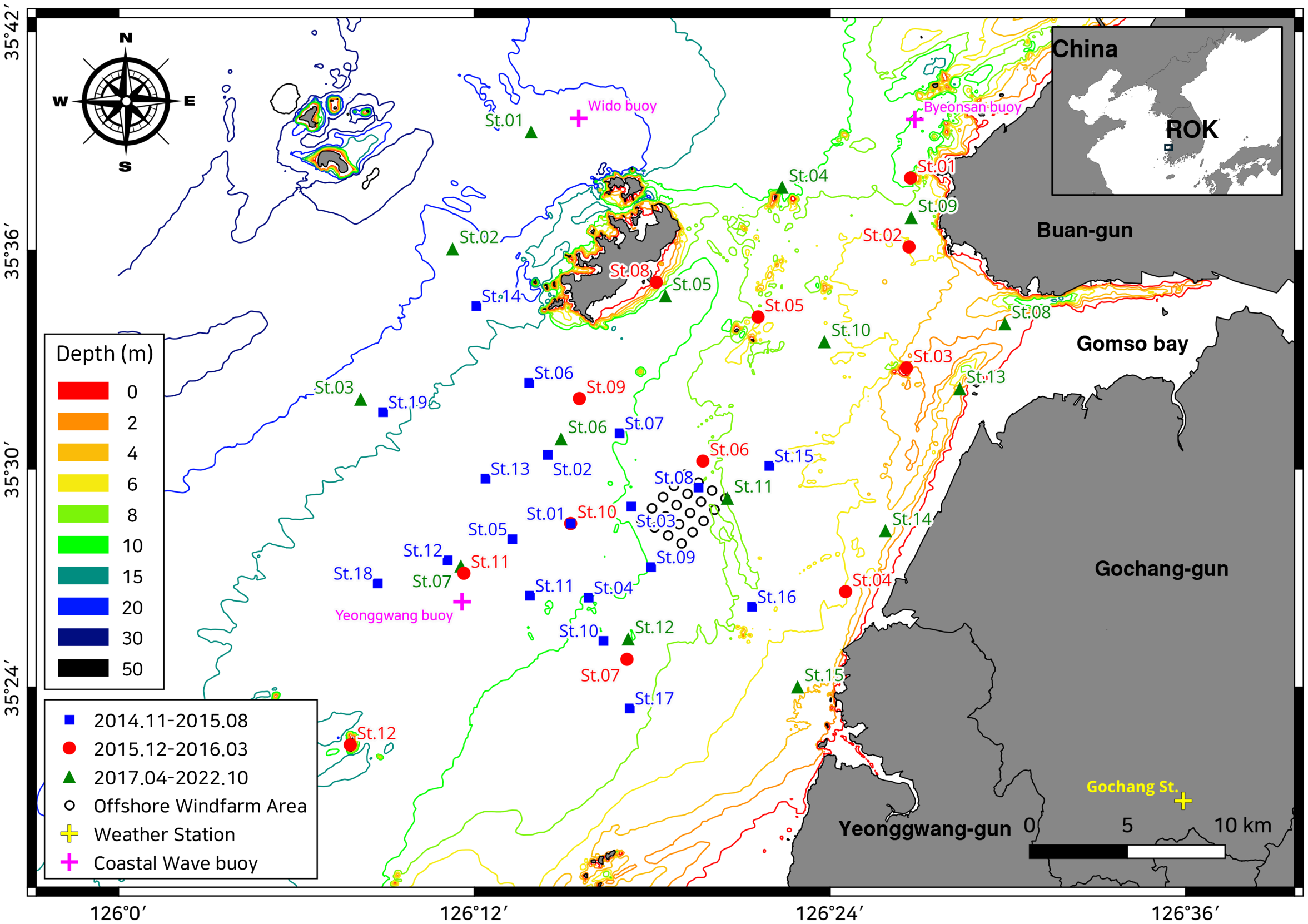
Index map depicting the sampling points in the preliminary effect assessment survey of the wind farm (2014–2015; blue squares), marine survey for industrial convergence facilities (2015–2016; red circles), and marine spatial environmental effect analysis of the wind farm and database construction (2017–2022, green triangles). The yellow and purple crosses indicate the location of the land weather station and coastal wave buoys (CWBs) where the wind speeds and significant wave heights, respectively, were measured. The 20 wind turbines are marked with black empty circles. The contour lines indicate bathymetric information based on the 1:25,000 scale coastal information map, referenced to datum level (approximately the lowest low water).
Korea has four distinct seasons and is influenced by the strong East Asian monsoonal climate. The East Asian monsoon is characterized by a distinct seasonal reversal of the monsoon wind flow driven by temperature differences between the Pacific Ocean and the East Asian continent (Ha et al., 2012). Along with the tidal regime, the seasonal variability of the monsoon system affects variations in hydrology and oceanographic processes, including sediment dispersal and deposition. Strong northwesterly winds prevail in winter (maximum wind speed of ~10 m/s), whereas relatively mild southeasterly winds occur during spring/summer accompanied by heavy rains (Frey et al., 1987; Yoo et al., 2010). Although summer storms are relatively shorter in duration than those in winter, strong winds occur in summer, with an average of two to three typhoons passing through the Yellow Sea per year (Hwang et al., 2014).
The Incheon coast, located in the northernmost part of the west coast of Korea, records a maximum monthly mean wind speed of >4 m/s in February and May (Frey et al., 1987). From 2014 to 2022, the maximum monthly mean wind speeds in the study area were recorded at Gochang weather station at 3.5 m/s in February 2016; at Yeonggwang weather station located 25 km further southwest, the maximum reading was 3.3 m/s in July 2013. However, these values were lower than the maximum recorded in Incheon (4.1 m/s in December 2014) during the same period (Korea Weather Web Portal, https://www.weather.go.kr/w/index.do).
The west coast of Korea has a flat seafloor topography with a continuous series of gently sloping tidal flats (Frey et al., 1987). Based on the coastal map issued by the Ministry of Oceans and Fisheries of Korea (scale 1:25 000), the depth of the Incheon coast, referenced to the datum level (approximately the lowest low water), was ~50 m within 40 km from land. For the Boryeong coast, located halfway between our study area and Incheon, where the wind farm is planned, the depth at 40 km offshore was ~56.3 m, with an average depth of approximately 30 m. Conversely, the study area was located within 30 km from the coast, with a depth of ~23 m and an average depth of 9.6 m, that is, shallower and narrower than other areas along the west coast (Figure 1).
Ocean bottom temperature data for the survey area, measured seasonally from 2002 to 2023, were retrieved from the Marine Environmental Information Web Portal (MEIS, https://www.meis.go.kr/mei/observe/port.do). The mean temperature was 15.4°C, with seasonal means of 4.0°C in February and 26.9°C in August. During the same period, the mean bottom salinity was 31.4 psu. The seasonal average was the highest in winter (31.7 psu), whereas the lowest in summer (30.8 psu), reflecting the influence of the summer monsoon on the bottom water. The surface sediment along the Korean west coast was primarily characterized by a broad distribution of fine to very fine sand (2–4 ϕ). However, the sediments in the study area were characterized by a grain size ranging at 3–7 ϕ, with silt sediment extending broadly southwestward from the very fine sand near the Geum estuary, located to the north of the study area (Cho et al., 1993).
Surface suspended particulate matter (SPM) concentrations along the Incheon coast were strongly influenced by tidal and wind-driven currents and ranged from 15 to 332 mg/L, with an average of 68.5 mg/L. The maximum and minimum seasonal averages were observed in February and June, respectively (Choi and Shim, 1986; Frey et al., 1987). According to the MEIS data from 2005 to 2023, the bottom SPM concentration in the study area showed similar trends over the years. The mean concentration was 34.9 mg/L, with highest and lowest seasonal averages observed in February (44.0 mg/L) and August (23.0 mg/L), respectively. During the given period, the minimum concentration was 1.6 mg/L in August 2014, whereas the maximum was 240.6 mg/L in November 2018.
The bottom dissolved oxygen (DO) saturation (%) is a parameter included in the five-grade evaluation system for Korean water quality index (WQI), with the thresholds for Grade II (good) and Grade III (moderate) being >80% and >67.5%, respectively (Park et al., 2019). The average and minimum values of the bottom DO saturation measured in the survey area were 95% and 65%, respectively. The 95% prediction lower bound, calculated as the mean minus two times the standard deviation, within which 95% of the observations lay, was 73%. Based on these results, the bottom DO saturation in the survey area could be classified, on average, as Grade I (very good), with 95% of the observations meeting at least a moderate status or better.
The maximum sediment total organic carbon (TOC) content in the study area was 1.17%, which was below the 1.5% threshold distinguishing “good” (Grade I) from “moderate” (Grade II) statuses in the four-grade criteria for assessing shellfish farm environments in Korea (Cho et al., 2013). The maximum sediment acid-volatile sulfide (AVS) concentration was 0.047 mg S/g dry weight, which was substantially lower than the optimal level of 0.25 mg S/g dry weight (Uede, 2008).
Although the maximum concentrations of most heavy metals in the sediment were below the effects range low (ERL) levels set by the United States Environmental Protection Agency, the maximum levels of cadmium, chromium, and nickel exceeded their corresponding ERL values of 1.2, 81.0, and 20.9 ppm, respectively. The average and 95% upper bound (upper two standard deviation) concentrations were 0.12 and 0.33 ppm, respectively, for cadmium; 52.2 and 83.6 ppm, respectively, for chromium; and 18.0 and 28.7 ppm, respectively, for nickel. The upper bound concentrations were approximately close to or below the ERL limits and well below the effects range median (ERM; 9.6, 370, and 51.6 ppm, respectively) levels. Thus, the study area was minimally contaminated by organic matter or heavy metals.
2.2 Field surveys and laboratory analysis
As shown in Figure 1, our survey points were established around the testbed of the Southwest Offshore Wind Farm project (Korea Offshore Wind Power Co. Ltd., KOWP; http://www.kowp.co.kr), located at the center of the study area. The area had 20 wind turbines. The OWF construction began in May 2017 and was completed in January 2020, after which the OWF has been continuously operating to date. Multiple pre- and post-project assessments were carried out for assessing environmental effects around the OWF.
The first monitoring program was the preliminary effect assessment survey of the wind farm, which was conducted at a total of 19 sampling points in four seasonal rounds from November 2014 to August 2015. The marine survey for industrial convergence facilities was performed at 12 points in three rounds from December 2015 to March 2016, before the installation of the structure. The marine spatial environmental effect analysis of the wind farm and database construction project, which covered both the construction and operation periods of the offshore wind structure, was conducted at 15 points in 21 rounds from June 2017 to October 2022.
For environmental data collection, we arrived at the sampling points by vessel. We measured the Secchi depth (m), bottom temperature (°C), salinity (psu), pH, DO (mg/L), and DO saturation (%) using a conductivity temperature depth (CTD) instrument (Ocean7 305, Idronaut, SRL, Brugherio, Italy). The depth (m) measurements varied depending on the time of observation because of the wide tidal range in the survey area; therefore, we utilized the measurements from the coastal map (scale 1:25 000) described above. For evaluating bottom-water environmental data, we collected samples at each point using a Niskin water sampler and transported them to the laboratory. In the laboratory, we measured the bottom SPM concentration (mg/L, filtering apparatus), chlorophyll-a content (Chl-a, µg/L, Fluorometer 10-AU, Turner Designs, San Jose, CA, USA), and chemical oxygen demand (COD, mg O2/L, potassium permanganate, titration method).
The top 1 cm of the sediment was sampled for textural and chemical analyses using a van Veen grab sampler at each sampling point. For the sedimentary textural analysis, the sediment sample was pretreated with hydrochloric acid and hydrogen peroxide to remove carbonate and organic matter, respectively.
Particle size analysis was performed by sieving and pipetting. Dry sand particles were analyzed using a hand-held sieve at 1.0 ϕ intervals, while mud particles were analyzed by pipetting at 1.0 ϕ intervals. The gravel, sand, silt, and clay contents (%) were calculated from the sediment grain size classification. Statistical parameters, such as mean grain size and sorting values, were calculated as described in the study by Folk and Ward (1957).
For the sediment organic matter content, ignition loss (%, Daehan Sci. Inc., Muffle Furnace FX-27, Wonju, Gangwon, Korea), TOC (mg/g, Thermo Fisher Scientific Inc., FLASH 2000, Waltham, MA, USA), total organic nitrogen (mg/g, Thermo Fisher Scientific Inc., FLASH 2000), and COD (mg/g, alkaline potassium permanganate method) were measured. Heavy metal (aluminum, iron, arsenic, cadmium, chromium, lithium, nickel, lead, copper, and zinc) concentrations (mg/kg) in the sediments were measured using the ELAN DRC II ICP-MS (Perkin-Elmer Inc., Shelton, CT, USA), and the derived metal concentrations, such as normalized copper and zinc levels, were calculated. In addition, the sediment AVS (mg S/g dry, hydrogen sulfide detector tube), which indicates organic matter content and sulfide toxicity, was measured.
At each sampling point, macrobenthos was collected twice using a van Veen grab sampler (surface sampling area, 0.1 m²). The sediment was filtered through a 1 mm mesh sieve using seawater, and the residue was transferred to a collection container and fixed with a 10% neutral formalin solution for transportation to the laboratory. In the laboratory, the samples were sorted and identified to the species or lowest possible taxonomic level using a stereomicroscope (Leica MZ125; Leica Microsystems, Wetzlar, Germany) and an optical microscope (Olympus BAC-313; Olympus Corporation, Tokyo, Japan). The abundance and wet weight of the biomass were measured for the identified taxonomic groups and expressed as values per unit area (m²). The scientific names of the identified taxa were standardized according to the World Register of Marine Species (WoRMS, https://www.marinespecies.org).
To incorporate weather-related variables into this study, we obtained weather data from the Data Service Center of the Korea Meteorological Administration (KMA, https://data.kma.go.kr/cmmn/main.do) at the Gochang weather station (marked by a yellow cross in Figure 1). This station was located near the study area, and data collection was performed using an automated synoptic observation system (ASOS). Monthly averages of daily significant wave heights were obtained from marine weather data provided by the KMA, recorded using three coastal wave buoys (CWBs) near the study area. As these three CWBs were located in Wido, Byeonsan, and Yeonggwang, the observations from the nearest CWB were assigned to each sampling point. The observation start date for the CWBs varied with location. Observations from Yeonggwang from November 2014 to March 2016 were assigned to all sampling points, whereas those from Byeonsan began in April 2017 and those from Wido in September 2018.
2.3 Data analysis
2.3.1 Data processing
Forty-two environmental factors were measured in this study. However, as missing values were present in the data matrix, we deleted variables or even whole data records (for example, the 2014 survey data) in the event of missing values. After addressing the missing value problem, the total number of database records consisting of community and environmental variables (described below) was reduced from 427 to 351, while that of environmental variables was reduced to 24.
A single widely used method for collecting weather-related variables and measurements of spatial variations in wind and waves could not be identified. The weather data, especially the wind data, used in this study were also measured at a limited number of locations. Thus, we used a quantitative but simple value in case of an unavailable survey round value to compare sampling points or distinguish spatial variations with different wave fetches. Ricciardi and Bourget (1999) adopted a similar approach.
The weather data included MeanWind and MaxWind (current monthly averages of daily mean and maximum wind speed, respectively; m/s), Hs (current monthly averages of daily significant wave height, m), HD (Hs/depth ratio; see below for further explanation), and Prev.Mean, Prev.Max, Prev.Hs, and Prev.HD (previous monthly averages of the four variables above). Previous monthly averages were used because the current monthly average included trailing data recorded after biological sampling; therefore, it was not causative. In addition, we assumed that previous monthly averages up to a month prior to biological sampling could be effective for the resulting response of the biological parameters observed in the current month.
We estimated and utilized the HD (Hs/depth ratio) as a composite variable for assessing the wave-induced forces affecting the bottom sediment. We followed the method by Seelam and Baldock (2012), who showed that the total shear stress (sum of form drag and bed shear) of a solitary wave is linearly related to the wave height/water depth.
To identify and quantify the effects of environmental factors on biological parameters, we targeted the diversity and wet weight of macrobenthic communities. We used Whittaker’s d, which allows for comparing the diversity to our past database with different surface sampling areas. The formula for the index was as follows:
where SRs is the total number of species in the sample, and A is the sample area in cm2 (Whittaker, 1975).
2.3.2 Benthic habitat mapping - sediment and biological parameters
We generated habitat maps that included bathymetric data, quantitative data on sediment distribution, and data on biological parameters of macrobenthic communities observed during the survey, using the 1:25,000 scale map described earlier. The bathymetric data referenced to the datum level consisted of 1559 points within the survey area. We used Surfer 25.1.220 (Golden Software, LLC, Golden, CO, USA) to integrate these data and create a digital elevation model (DEM), using the kriging algorithm as the interpolation method. The raster grid resolution of the bathymetric DEM was set to 25 m.
For analyzing the sediment and biological parameters, we used the inverse distance weighted (IDW) interpolation algorithm, which is more suitable than the kriging algorithm for sparse or irregular data distributions (Munyati and Sinthumule, 2021). The weighting factor (P), which determines the influence of nearby sampling points on the interpolation values, was set to 2.0, and the raster grid resolution was set to 25 m.
The habitat maps with bathymetric information included 12–19 sampling points per survey round using the: (1) sediment mean grain size data (ϕ), (2) Whittaker’s index for diversity, and (3) logarithmically transformed wet weight biomass, b (log b+1, base10) for the biomass.
Regarding the assessment of macrobenthic community biomass, unlike Whittaker’s d or species number, which lack previously established criteria for categorizing diversity levels in Korea, various criteria are available for distinguishing low levels of biomass. Jeong et al. (2019) estimated the log-transformed Q1 value to be 1.0 (9.10 g/m²), indicating low biomass on the west Coast of Korea. In this study, we estimated the Q1 of Whittaker’s d from the same data set (n = 372, surface sampling area = 0.3 m² per sampling point) to be 6.6 and used this value for the same purpose.
We examined the spatial patterns of diversity and biomass by classifying the areas as anomalous if any value was lower than the abovementioned threshold and as normal if not. To categorize the survey rounds as normal or anomalous, we counted the number of sampling points with diversity and biomass anomalies and classified each round as anomalous if the proportion was 33.3% or higher. Although this threshold was not derived from a formal ecological standard, it was selected as a conservative empirical criterion to identify survey rounds in which anomalies were not confined to a few isolated stations but instead occurred across a broader spatial extent. Sensitivity analyses across a range of cutoff values (0.05–0.70) confirmed the robustness of this criterion, as it consistently distinguished anomalous from normal rounds with statistically significant differences (p< 0.001) and large effect sizes (Cliff’s delta ≥ |0.5|) in the station-level distributions of diversity and biomass.
2.3.3 Multiple regression analysis
Given the high variability and nonlinearity of biological parameters, Whittaker’s d and wet weight biomass were transformed using square root and consecutive logarithmic transformations (log ((log b + 1) + 1)), respectively. As anticipated, the 24 aforementioned environmental factors were highly correlated. To address the multicollinearity problem that may arise from these high correlations among the predictors in the multiple regression analysis, we conducted a Pearson’s correlation analysis prior to model estimation. If the absolute correlation values between two variables were greater than 0.5 (|r| > 0.5), we eliminated the variable that had a lower correlation with the biological parameters (Yoo et al., 2013). We then prepared a set of variables for the regression analysis and performed the best subsets regression to identify a useful subset of predictors using Minitab 21 (Minitab, LLC, State College, PA, USA).
While exploring various models from the output of the best subsets regression, we focused on Mallows’ Cp, which helps select a model that is both accurate and unbiased by looking for the smallest difference between the Cp value and total number of predictors plus a constant. In addition, we considered the predicted R², which indicates the predictive ability of the model. We identified two or more models that satisfied these two criteria, and ultimately, chose the regression model with the highest R² value. Most models selected based on these criteria had few predictors and demonstrated either a high predicted R² or a value close to it. This was also true for the adjusted R², which provides insights into potential overfitting.
For the selected models, each predictor was standardized by subtracting the mean and dividing it by the standard deviation. This method allowed us to easily compare the sizes of the coefficient estimates and determine the predictors with a large effect. We used these standardized predictors to fit the model and compared the regression coefficients among the predictors using graphs. Unstandardized regression coefficients and additional statistics, such as the F-test, variance inflation factors, R², and model equations, are presented in the ANOVA tables.
We examined the Pearson correlation between the macrobenthic community parameters and weather-related variables (hereafter referred to as air predictors). This was performed (1) to assess the validity of the estimated effects of air predictors in the regression analysis by checking the consistency between the sign and size of beta estimates and the correlation in case of no prior information on the effects of air predictors and (2) to distinguish air predictors that were effective but eliminated during the variable selection process because of high correlation with other predictors.
We classified the environmental factors into marine environmental predictors (hereafter referred to as sea predictors) and weather-related air predictors and prepared two types of datasets, one consisting of sea predictors and the other consisting of both air and sea predictors, to conduct a step-by-step regression analysis. We investigated whether the additive inclusion of air predictors in the model resulted in statistical improvements and ecological significance. Model estimation based on air–sea predictors was also conducted separately for two types of data: individual sampling point and survey round-averaged data. Averaged data were used to leverage the central tendency of the environmental data and biological parameters and to eliminate the effect of spatial variation.
To assess the performance of the regression models, we calculated the Pearson correlation coefficient between the observed and predicted values and examined the changes in the correlation coefficients associated with the addition of air predictors. The categories for the correlation coefficients were based on the findings by Chen et al. (2021), where |r| ≤ 0.3 was considered negligible, 0.3< |r| ≤ 0.5 was weak, 0.5< |r| ≤ 0.7 was moderate, 0.7< |r| ≤ 0.9 was strong, and 0.9< |r| ≤ 1 was fully correlated.
2.3.4 Seasonal mean model and logistic regression analysis
To understand the seasonal variations in biological parameters, we selected one of the air predictors based on the results of the regression analysis and estimated the seasonality of the predictor and biological parameters. We categorized the survey rounds into four seasons (spring = 1, summer = 2, fall = 3, and winter = 4), and applied a seasonal mean model, expressed as follows:
is the indicator variable defined as
= 1, when t or
0, when ,… where .
Employing the indicator variables, we estimated the seasonal model using regression analysis with no intercept option for the residual average as 0 (Choi, 1992) and then identified seasonality using beta estimates corresponding to the seasonal mean. Linear trends were fitted to the deseasonalized residuals, and Pearson correlations between the environmental factor and biological parameter residuals were analyzed.
We predicted the conditions of occurrence for the anomaly survey round (proportion of anomaly samples per a survey round ≥33%) using multiple logistic regression with air predictors. In the analysis, the response variables, namely, survey rounds, were coded as 1 for anomalies and 0 for normal responses. Prior to analysis, the linear relationship between the proportion of anomalous samples per survey round of diversity and biomass was estimated. Thereafter, we examined the differences in the proportions of anomaly samples in a survey round based on diversity vs. biomass and the differences of each parameter between anomaly vs. normal using a Spear style boxplot without upper and lower fence (upper and lower quartile ± 1.5 interquartile range). The Levene’s test for equal variances and t-test for equal means were performed to test for statistical differences.
We employed a stepwise procedure and selected the final set of predictors and models based on the significance of the Wald test. We examined the deviance R2, which indicates the variations explained by the model, and the area under the ROC curve (AUC) to determine the fitting of the data in the model. The AUC indicates the efficiency by which the binary model can separate the classes and ranges between 0.5 and 1. A value of 0.5 indicated that the model could not separate the classes better than a random assignment. The Wald test was used to test the hypothesis that the set of beta coefficients is equal to zero.
3 Results
3.1 Benthic habitat map
The mean sediment grain size distribution in the study area is presented in a benthic habitat map (Figure 2). Mixed sand-silt to silt sediments were primarily present, with grain sizes ranging from 4–5 to 7 ϕ. Exceptionally, fine sand (approximately 3 ϕ) and fine silt sediments (approximately 7 ϕ) were observed temporarily in the southern and northern parts of the area, respectively, in October and November 2018. SPM data from November 2018 coincided with the maximum bottom SPM concentration from the web portal (MEIS) data and our SPM observation over the 97th percentile at the southeastern sampling point (St. 15, 176.4 mg/L).
Figure 2
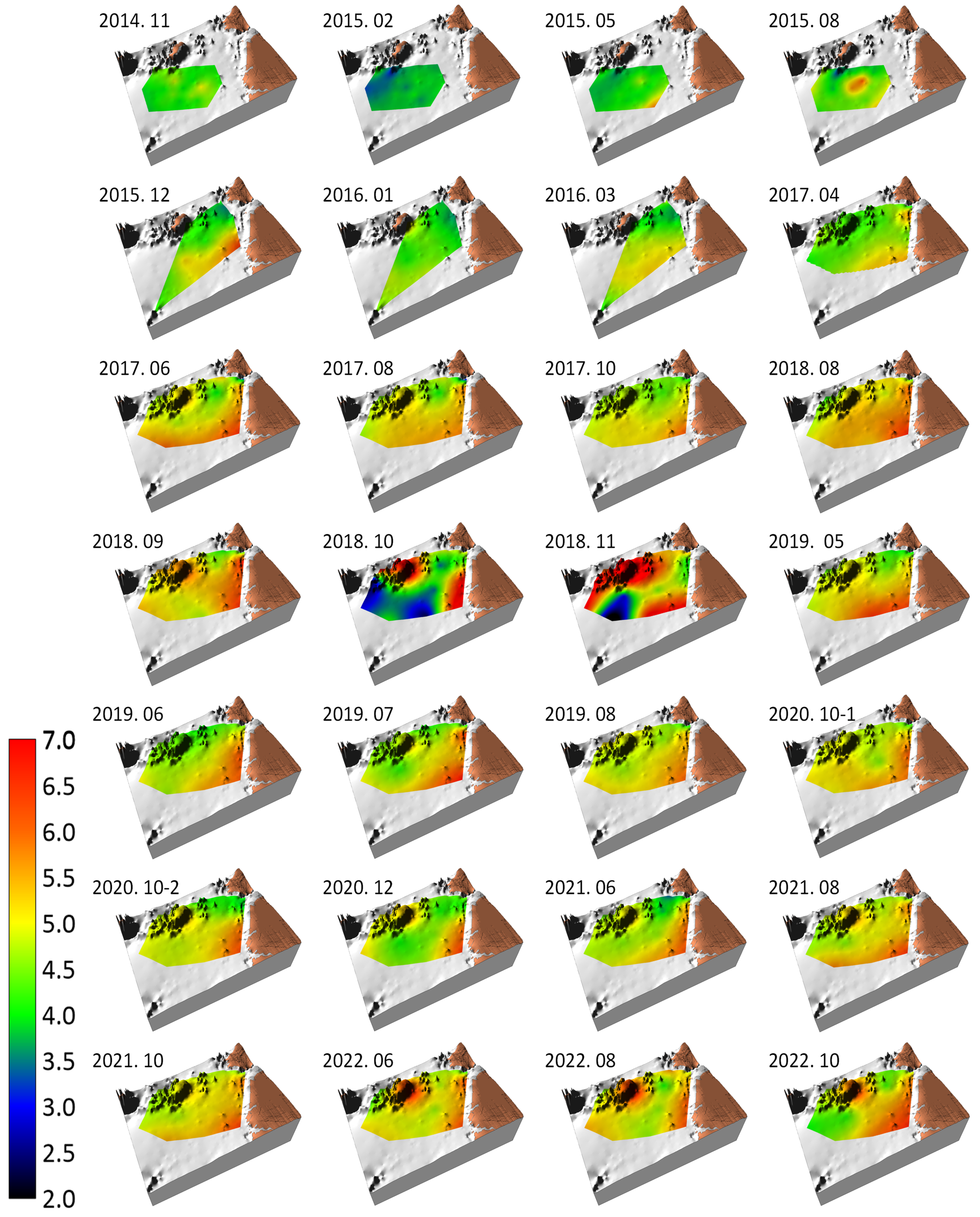
Benthic habitat map showing topography and spatiotemporal variation of the mean grain size (ϕ) of the bottom sediment of the study area from November 2014 to October 2022. The color palette on the left shows the mean grain size range from 2.0 to 7.0 ϕ.
Initially, the sediment grain size ranged at 4–5 ϕ (sand-silt mixed sediment), but as the survey progressed, the spatial occupancy/frequency of muddy sediments (greater than 5.5 ϕ) became predominant in the shallower southeastern part of the surveyed area. Temporary changes in the mean sediment grain size were observed in the middle of the survey. In October and November, 2018, sediment fining (red hues) was observed in the northwestern part of the surveyed area, whereas coarsening (blue hues) was observed in the southern part, with distinct sediment distribution patterns detected before and after this period. After this period, a strengthening of the red hues was observed in the sediment distribution in this area, indicating that the sediments in the shallower southeastern part became muddier over time.
Macrobenthic diversity (Whittaker’s d) is presented in a benthic habitat map (Figure 3). Blue/darker hues, which generally appeared between February 2015 and June 2017, correspond to anomalous diversity (d = 6.6). In addition, a consistently low diversity was observed in the shallower southeastern part of the surveyed area at times and locations of occurrence of mud bottoms (Figure 2). From August 2017, the diversity increased compared with that in previous years, with that in June 2022 being an exception. Anomaly rounds accounted for 28.6% of all survey rounds (left inset of the bar graph in Figure 3).
Figure 3
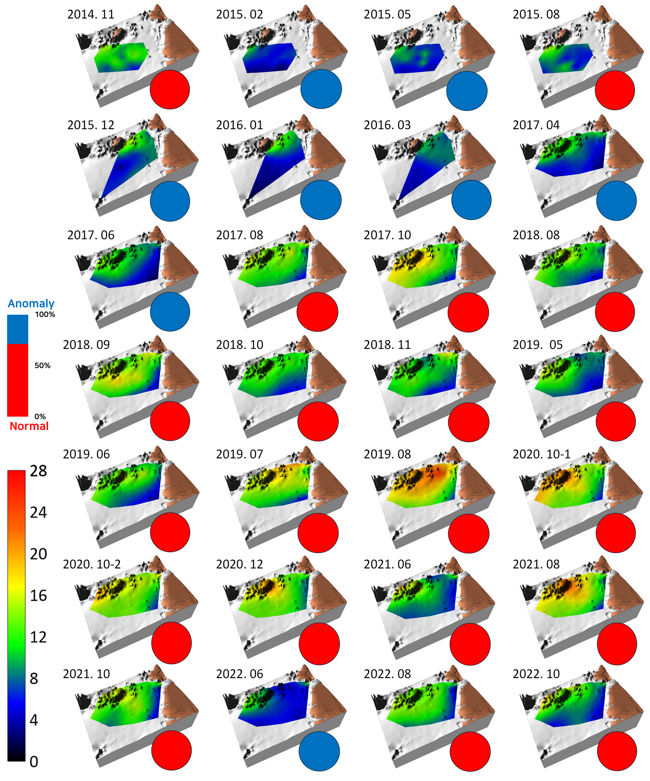
Benthic habitat map showing the topography, spatiotemporal variation in the diversity of macrobenthic communities (Whittaker’s d), and ratio of normal (red circle) vs. anomalous (blue circle) survey rounds observed in the study area from November 2014 to October 2022. The color palette on the left side shows the range of Whittaker’s d from 0 to 28, while the bar graph above it represents the proportion of normal to anomaly survey rounds.
The log-transformed wet-weight biomass of the macrobenthic communities present in the benthic habitat map is shown in Figure 4. Relatively high biomass was observed during the early survey periods of November 2014 and August 2015; however, dark green/darker hues, indicating biomass anomalies, were predominantly observed until June 2017. Following this period, a bright green color, representing biomass in the range of approximately 25–100 g/m² (log scale bar, approximately 1.4–2.0), became predominant, reflecting an increase in biomass. Toward the later stages of the survey, dark green/dark hues reappeared, suggesting a gradual decline in biomass. This pattern appeared to roughly align with the fluctuations observed in diversity.
Figure 4
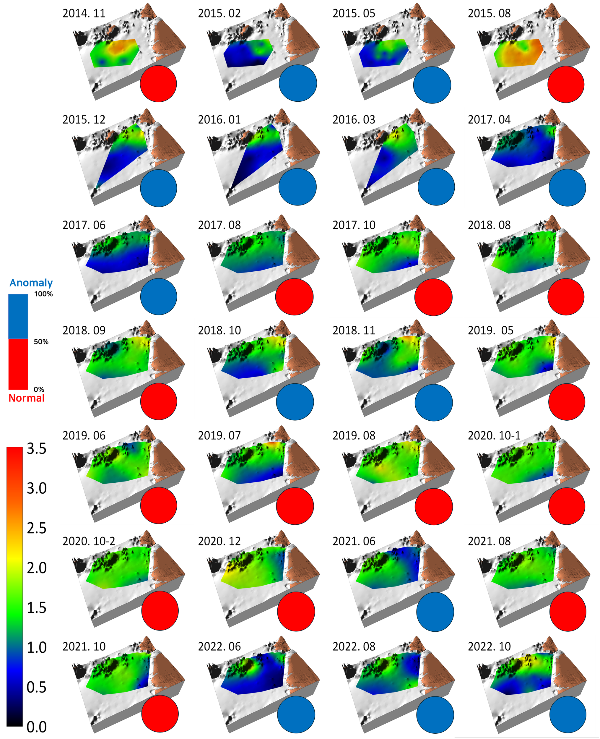
Benthic habitat map showing the topography, spatiotemporal variation of log-transformed wet weight, biomass of macrobenthic communities, and ratio of normal (red circles) vs. anomaly survey rounds (blue circles) observed in the study area from November 2014 to October 2022. The color palette on the left side shows the range of log-transformed biomass from 0 to 3.5, while the bar graph above it represents the proportion of normal to anomaly survey rounds.
Biomass anomalies showed little regularity. The occurrence of anomalies partially coincided with periods of low diversity (e.g., February 2015 to June 2017 and June 2022) and times at which the spatial distribution of sediment changed from that in previous surveys. During such changes, for instance, after the predominant distribution of mixed sediments, sand bottoms emerged in some areas, resulting in a color change on the map from green to blue (e.g., February 2015, October and November 2018). Mud bottoms (red hues in the map) sometimes expanded in the shallower southeastern part (e.g., December 2015 and June 2017) or when the previously homogeneous sediment distribution became heterogeneous (e.g., October and November 2018 and June, August, and October 2022), all of which aligned with the emergence of anomalies. Anomaly rounds accounted for 46.4% of all survey rounds (left inset of the bar graph in Figure 4).
3.2 Linear regression using sea predictors
Square root-transformed Whittaker’s d (Sqrt d) was positively correlated with log-transformed sand content (log sand) (Figure 5A). Log sand was highly correlated with mean grain size (MGS, r = -0.84, p< 0.001). Sqrt d was also positively correlated with depth and negatively correlated with DO (r = -0.76, p< 0.001 with temperature), salinity (r = -0.50, p< 0.001 with Chl-a; r = 0.19, p< 0.001 with depth; and r = 0.18, p = 0.001 with temperature) and log SPM (r = 0.286, p< 0.001 with sediment log TOC). The correlation coefficient between the observed and predicted values was moderate (r = 0.68, p< 0.001) (Figure 5C).
Figure 5
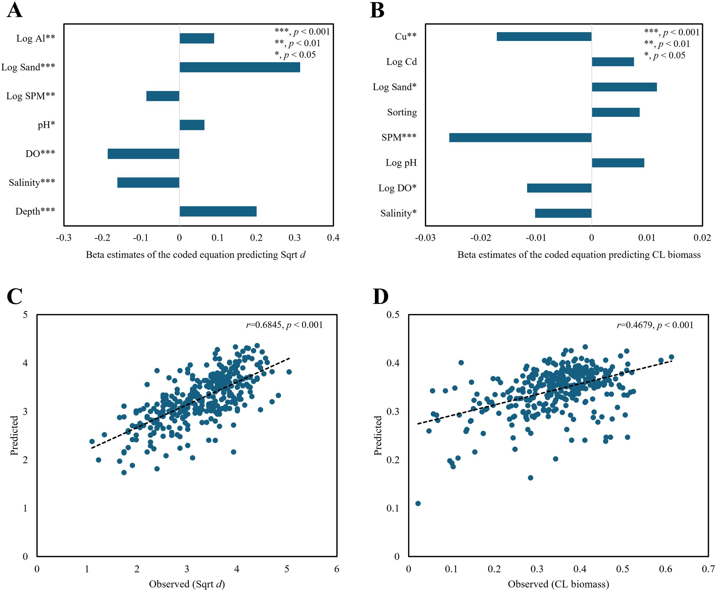
Regression plots of macrobenthic diversity with Sqrt d (square root-transformed Whittaker’s d) and CL biomass (consecutively log-transformed wet weight, g/m²) using sea predictors (bottom water/sediment variables). Beta estimates of the coded equations (A, B) and observed-predicted plots for the diversity and biomass regression models (C, D). Log indicates log-transformation for variable x (log (x + 1), base = 10), Al (sediment aluminum concentration), Sand (sand content), SPM (suspended particulate matter), pH (power of hydrogen), DO (dissolved oxygen), Cu (copper in sediment), Cd (cadmium in sediment), and Sorting (sediment sorting). Asterisks indicate statistical significance (*p < 0.05; **p < 0.01; *p < 0.001).
SPM and sediment copper (Cu) had significant negative effects on consecutive log-transformed biomass (CL biomass) (Figure 5B). Cu exhibited a high correlation with substratum properties, such as log sand (r = -0.42, p< 0.001), MGS (r = 0.37, p< 0.001), ignition loss (r = 0.60, p< 0.001), and sediment TOC (r = 0.51, p< 0.001). The correlation between the observed and predicted biomass values was weak (r = 0.47, p< 0.001) (Figure 5D).
Table 1 presents a summary of the regression analysis results. The diversity of the macrobenthic communities in the surveyed area was adequately explained by seven predictors, all of which were significant at a p-value of 0.05. The coefficient of determination R² was 0.47, with significance set at p< 0.001. The collinearity statistics, represented by variance inflation factors (VIFs), were all satisfactory, below 1.3. The R² value for the biomass regression model was 0.22, which was statistically significant (p< 0.001). Among the eight predictors, log-transformed bottom pH (log pH), sediment sorting, and log-transformed sediment Cd (log Cd) were insignificant, whereas the remaining five predictors showed statistical significance (p< 0.05). All VIFs were satisfactory.
Table 1
| Regression for Sqrt d | ||||||
|---|---|---|---|---|---|---|
| Source | DF | Adj SS | Adj MS | F-value | P-value | VIF |
| Regression | 7 | 88.141 | 12.592 | 43.19 | 0.000 | – |
| Depth | 1 | 12.625 | 12.625 | 43.3 | 0.000 | 1.12 |
| Salinity | 1 | 7.667 | 7.667 | 26.3 | 0.000 | 1.19 |
| DO | 1 | 9.627 | 9.627 | 33.02 | 0.000 | 1.26 |
| pH | 1 | 1.330 | 1.330 | 4.56 | 0.033 | 1.12 |
| Log SPM | 1 | 2.037 | 2.037 | 6.99 | 0.009 | 1.27 |
| Log Sand | 1 | 29.298 | 29.298 | 100.49 | 0.000 | 1.18 |
| Log Al | 1 | 2.506 | 2.506 | 8.6 | 0.004 | 1.13 |
| Error | 343 | 100.003 | 0.292 | – | – | – |
| Total | 350 | 188.144 | - | - | - | - |
| Model Summary | S | R2 | R2 (adj) | R2 (pred) | ||
| 0.539956 | 0.4685 | 0.4576 | 0.4446 | |||
| Regression equation in uncoded units: | ||||||
| Sqrt d = 3.984 + 0.03437 Depth - 0.1036 Salinity - 0.1333 DO + 0.1226 pH - 0.2308 Log SPM + 1.032 Log Sand + 1.057 Log Al | ||||||
| Regression for CL biomass | ||||||
|---|---|---|---|---|---|---|
| Source | DF | Adj SS | Adj MS | F-value | P-value | VIF |
| Regression | 8 | 0.74995 | 0.09374 | 11.98 | 0.000 | – |
| Salinity | 1 | 0.03466 | 0.03466 | 4.43 | 0.036 | 1.05 |
| Log DO | 1 | 0.03839 | 0.03839 | 4.91 | 0.027 | 1.24 |
| Log pH | 1 | 0.02872 | 0.02872 | 3.67 | 0.056 | 1.1 |
| SPM | 1 | 0.19164 | 0.19164 | 24.5 | 0.000 | 1.21 |
| Sorting | 1 | 0.02275 | 0.02275 | 2.91 | 0.089 | 1.16 |
| Log Sand | 1 | 0.03598 | 0.03598 | 4.6 | 0.033 | 1.34 |
| Log Cd | 1 | 0.01914 | 0.01914 | 2.45 | 0.119 | 1.07 |
| Cu | 1 | 0.07903 | 0.07903 | 10.1 | 0.002 | 1.3 |
| Error | 342 | 2.67528 | 0.00782 | – | – | – |
| Total | 350 | 3.42522 | - | - | - | - |
| Model Summary | S | R2 | R2 (adj) | R2 (pred) | ||
| 0.0884446 | 0.2189 | 0.2007 | 0.168 | |||
| Regression equation in uncoded units: | ||||||
| CL Biomass = 0.337 - 0.00655 Salinity - 0.1693 Log DO + 0.339 Log pH - 0.000542 SPM + 0.0216 Sorting + 0.0387 Log Sand + 0.222 Log Cd - 0.00363 Cu | ||||||
Analysis of variance for the diversity and biomass regression models based on sea predictors (bottom water/sediment variables).
Log indicates log-transformation for variable x (log (x + 1), base = 10), DO (dissolved oxygen, mg/L), pH (power of hydrogen), SPM (suspended particulate matter, mg/L), Sand (sand content, %), Al (sediment aluminum concentration, mg/Kg), Sorting (sediment sorting, ϕ), Cd (cadmium in sediment, mg/Kg), and Cu (copper in sediment, mg/Kg).
3.3 Linear regression using air–sea predictors
The air predictors that exhibited significant correlations with diversity were MeanWind, MaxWind, Hs, Prev.Hs, and Prev.HD (Figure 6A). Prev.Hs and Prev.HD showed high correlation coefficients with Hs (r = 0.65, p< 0.001) and HD (r = 0.88, p< 0.001). The variables that demonstrated significant correlations with the biomass were MeanWind, MaxWind, Hs, Prev.Mean, and Prev.Hs. Among them, MeanWind exhibited a notable correlation (r = -0.41, p< 0.001) with diversity (Figure 6B). Most air predictors were significant and displayed negative relationships with the biological parameters.
Figure 6
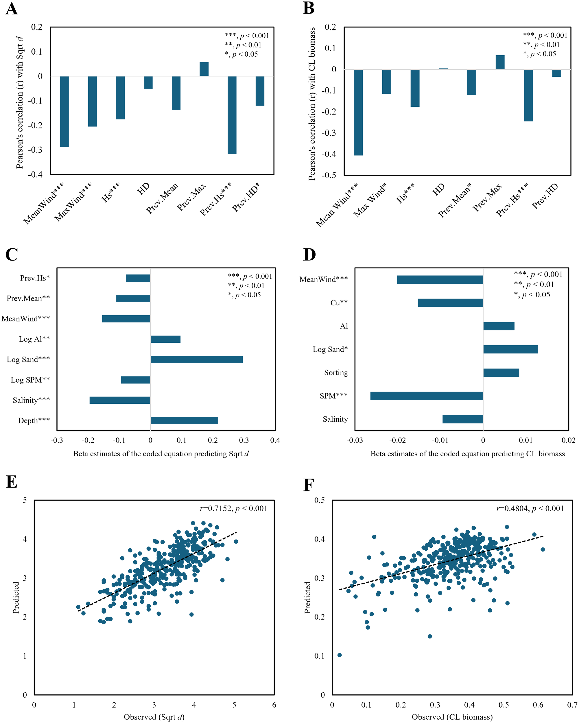
Regression plots of macrobenthic diversity with Sqrt d (square root-transformed Whittaker’s d) and CL biomass (consecutively log-transformed wet weight, g/m²) using air–sea predictors (bottom water/sediment and wind/wave variables). Correlations of macrobenthic diversity and biomass with air predictors, namely, MeanWind, MaxWind, Hs, and HD (current monthly averages of daily mean, maximum wind speed, significant wave height, and Hs/depth ratio), and Prev.Mean, Prev.Max, Prev.Hs, and Prev.HD (previous monthly MeanWind, MaxWind, Hs, and HD) (A, B). Beta estimates of the coded equations (C, D) and observed-predicted plots for the diversity and biomass regression models (E, F). Asterisks indicate statistical significance (*p < 0.05; **p < 0.01; *p < 0.001).
The diversity regression model shown in Figure 6C revealed that significant sea predictors were log sand, depth, salinity, and log SPM. In this regard, the results shown in Figure 6C are similar to those in Figure 5A. DO, included in Figure 5A, was excluded from the analysis because of its high correlation with the air predictor Prev.Hs (r = 0.64, p< 0.001). Although air predictors had lower effects than sea predictors (i.e., log sand, salinity, and depth), the mean and Prev.Hs had significant negative effects on diversity.
Among the sea predictors in the biomass regression model, SPM demonstrated the most significant effect, with Cu and log sand also included as significant variables, indicating a similarity with the results of the sea predictor-based model shown in Figure 5B and Table 1. Log DO was excluded from the variable selection because of its significant correlations with several factors, including SPM (r = 0.30, p< 0.001), MeanWind (r = 0.43, p< 0.001), and Prev.Mean (r = 0.31, p< 0.001). The only air predictor included was MeanWind, whose effect was estimated to be greater than that of Cu (Figure 6D).
The correlation coefficients between the observed and predicted values in the diversity and biomass prediction models that included air predictors were 0.72 (p< 0.001) and 0.48 (p< 0.001), respectively. The numbers of predictors in these models were eight and seven, respectively, similar to those in the sea predictor-based models (seven and eight, respectively) (Tables 1, 2). Although not substantial, an increase was observed in the correlation coefficients between the observed and predicted values of the models. The correlation coefficient range for the diversity model shifted from moderate to strong (Figures 6E, F).
Table 2
| Regression for Sqrt d | ||||||
|---|---|---|---|---|---|---|
| Source | DF | Adj SS | Adj MS | F-value | P-value | VIF |
| Regression | 8 | 96.241 | 12.030 | 44.77 | 0.000 | – |
| Depth | 1 | 15.043 | 15.043 | 55.98 | 0.000 | 1.10 |
| Salinity | 1 | 10.496 | 10.496 | 39.06 | 0.000 | 1.27 |
| Log SPM | 1 | 2.530 | 2.530 | 9.41 | 0.002 | 1.23 |
| Log Sand | 1 | 27.795 | 27.795 | 103.43 | 0.000 | 1.10 |
| Log Al | 1 | 2.899 | 2.899 | 10.79 | 0.001 | 1.12 |
| MeanWind | 1 | 7.243 | 7.243 | 26.95 | 0.000 | 1.16 |
| Prev.Mean | 1 | 2.989 | 2.989 | 11.12 | 0.001 | 1.45 |
| Prev.Hs | 1 | 1.511 | 1.511 | 5.62 | 0.018 | 1.43 |
| Error | 342 | 91.904 | 0.269 | – | – | – |
| Total | 350 | 188.144 | – | - | - | - |
| Model Summary | S | R2 | R2 (adj) | R2 (pred) | ||
| 0.518386 | 0.5115 | 0.5001 | 0.4857 | |||
| Regression equation in uncoded units: | ||||||
| Sqrt d = 6.932 + 0.03726 Depth - 0.1253 Salinity - 0.2530 Log SPM + 0.9730 Log Sand + 1.129 Log Al - 0.541 MeanWind - 0.3108 Prev.Mean - 0.313 Prev.Hs | ||||||
| Regression for CL biomass | ||||||
|---|---|---|---|---|---|---|
| Source | DF | Adj SS | Adj MS | F-value | P-value | VIF |
| Regression | 7 | 0.79061 | 0.11295 | 14.7 | 0.000 | – |
| Salinity | 1 | 0.02859 | 0.02859 | 3.72 | 0.055 | 1.11 |
| SPM | 1 | 0.21322 | 0.21323 | 27.76 | 0.000 | 1.14 |
| Sorting | 1 | 0.02302 | 0.02302 | 3.00 | 0.084 | 1.08 |
| Log Sand | 1 | 0.04314 | 0.04314 | 5.62 | 0.018 | 1.31 |
| Al | 1 | 0.01689 | 0.01689 | 2.20 | 0.139 | 1.11 |
| Cu | 1 | 0.06256 | 0.06256 | 8.15 | 0.005 | 1.3 |
| MeanWind | 1 | 0.12821 | 0.12821 | 16.69 | 0.000 | 1.11 |
| Error | 340 | 2.44871 | 0.00720 | – | – | – |
| Total | 350 | 3.42522 | - | - | - | - |
| Model Summary | S | R2 | R2 (adj) | R2 (pred) | ||
| 0.0876418 | 0.2308 | 0.2151 | 0.1882 | |||
| Regression equation in uncoded units: | ||||||
| CL Biomass = 0.632 - 0.00610 Salinity - 0.000555 SPM + 0.0210 Sorting + 0.0418 Log Sand + 0.00486 Al - 0.00324 Cu - 0.0703 MeanWind | ||||||
Analysis of variance for the diversity and biomass regression models based on air–sea predictors (bottom water/sediment and wind/wave variables).
Log indicates log-transformation for variable x (log (x + 1), base = 10), SPM (suspended particulate matter, mg/L), Sand (sand content, %), Al (sediment aluminum concentration, mg/Kg), Sorting (sediment sorting, ϕ), Cu (copper in sediment, mg/Kg), MeanWind (current monthly averages of daily mean wind speed; m/s), Prev.Mean (previous monthly MeanWind; m/s), and Prev.Hs (previous averages of daily significant wave height; m).
The predictors of diversity for macrobenthic communities in the surveyed area were mostly significant (p< 0.001), with all VIFs being below 1.5, indicating good multicollinearity. This model was statistically significant (p< 0.001; Table 2). In addition, the biomass regression model was also significant (p< 0.001), with SPM and MeanWind appearing significant (p< 0.001) and VIFs being at a very satisfactory level (Table 2).
3.4 Averaged parameters and air–sea predictors
The air predictors that were significantly correlated with survey-averaged diversity included MeanWind (r = -0.51, p = 0.006), Prev.Hs (r = -0.54, p = 0.003), and Prev.HD (r = -0.41, p = 0.029) (Figure 7A). The predictors that exhibited significant correlations with survey-averaged biomass were the same as those for diversity, namely MeanWind (r = -0.71, p< 0.001), Prev.Hs (r = -0.39, p = 0.038), and Prev.HD (r = -0.42, p = 0.028) (Figure 7B).
Figure 7
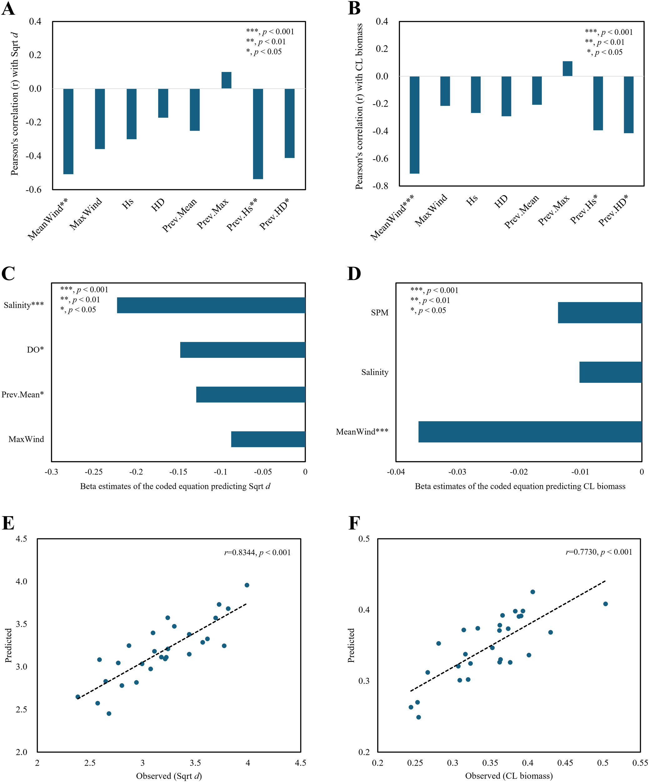
Regression plots of average macrobenthic diversity from survey rounds with Sqrt d (square root-transformed Whittaker’s d) and CL biomass (consecutively log-transformed wet weight, g/m2) using air–sea predictors (bottom water/sediment and wind/wave variables). Correlations of macrobenthic diversity and biomass with air predictors, namely, MeanWind, MaxWind, Hs, and HD (current monthly averages of daily mean, maximum wind speed, significant wave height, and Hs/depth ratio), and Prev.Mean, Prev.Max, Prev.Hs, and Prev.HD (previous monthly MeanWind, MaxWind, Hs, and HD) (A, B). Beta estimates of the coded equations (C, D) and observed-predicted plots for the diversity and biomass regression models (E, F). Asterisks indicate statistical significance (*p < 0.05; **p < 0.01; *p < 0.001).
In the average diversity regression model, salinity (r = -0.67, p< 0.001 with Chl-a) and DO had relatively large effects among sea predictors. Prev.Mean was the only significant variable among air predictors, showing a lower effect than that of other predictors (Figure 7C). MeanWind, which was only moderately correlated with Sqrt d (Figure 7A), was replaced by DO, which was highly correlated with Sqrt d (r = -0.63, p< 0.001), during the variable selection prior to the regression analysis. In the average biomass regression model, MeanWind was the only significant air predictor (p< 0.001) of biomass (Figure 7D).
DO showed higher correlations with most air predictors (e.g., r = 0.56, p = 0.002 with MeanWind; r = 0.67, p< 0.001 with Hs; r =0.83, p< 0.001 with Prev.Hs; r = 0.56, p = 0.002 with HD; r = 0.74, p< 0.001 with Prev.HD). In contrast, salinity showed seasonal variability, correlating best with MaxWind (r = 0.361, p = 0.059), whereas none of the other air predictors were significantly correlated with salinity.
The Pearson correlation coefficients between the observed and predicted values of the survey-averaged diversity and biomass regression models were r = 0.83 (p< 0.001) and r = 0.77 (p< 0.001), respectively. The model predicting diversity, which included four predictors, was significant (p< 0.001), with all VIFs being satisfactory at 1.6 or below. The biomass regression model, which included three predictors, was also significant (p< 0.001), with VIFs close to 1, indicating an excellent level for avoiding multicollinearity (Figures 7E, F; Table 3). The correlation coefficient for the diversity model remained within a strong range, whereas that for the biomass model varied from weak to strong (Figures 7E, F).
Table 3
| Regression for Sqrt d | ||||||
|---|---|---|---|---|---|---|
| Source | DF | Adj SS | Adj MS | F-value | P-value | VIF |
| Regression | 4 | 3.3925 | 0.84814 | 13.18 | 0.000 | – |
| MaxWind | 1 | 0.1485 | 0.14851 | 2.31 | 0.142 | 1.4 |
| Prev.Mean | 1 | 0.2856 | 0.28557 | 4.44 | 0.046 | 1.57 |
| DO | 1 | 0.3992 | 0.39918 | 6.2 | 0.020 | 1.48 |
| Salinity | 1 | 1.0644 | 1.06439 | 16.54 | 0.000 | 1.26 |
| Error | 23 | 1.48 | 0.06435 | – | – | – |
| Total | 27 | 4.8726 | – | – | – | – |
| Model Summary | S | R2 | R2 (adj) | R2 (pred) | ||
| 0.25367 | 0.6963 | 0.6434 | 0.5585 | |||
| Regression equation in uncoded units: | ||||||
| Sqrt d = 10.67 - 0.0400 Max Wind - 0.360 Prev.Mean - 0.1063 DO - 0.1691 Salinity | ||||||
| Regression for CL biomass | ||||||
|---|---|---|---|---|---|---|
| Source | DF | Adj SS | Adj MS | F-value | P-value | VIF |
| Regression | 3 | 0.055624 | 0.018541 | 11.88 | 0.000 | – |
| MeanWind | 1 | 0.032097 | 0.032097 | 20.56 | 0.000 | 1.11 |
| Salinity | 1 | 0.002651 | 0.002651 | 1.7 | 0.205 | 1.05 |
| SPM | 1 | 0.004381 | 0.004381 | 2.81 | 0.107 | 1.15 |
| Error | 24 | 0.037468 | 0.001561 | – | – | – |
| Total | 27 | 0.093092 | – | – | – | - |
| Model Summary | S | R2 | R2 (adj) | R2 (pred) | ||
| 0.0395116 | 0.5975 | 0.5472 | 0.4684 | |||
| Regression equation in uncoded units: | ||||||
| CL Biomass = 0.894 - 0.1171 MeanWind - 0.00772 Salinity - 0.000333 SPM | ||||||
Analysis of variance for the survey round-averaged diversity and biomass regression models based on air–sea predictors (bottom water/sediment and wind/wave variables).
MaxWind (current monthly averages of daily maximum wind speed; m/s), MeanWind and Prev.Mean (current and previous monthly averages of daily mean wind speed, respectively; m/s), DO (dissolved oxygen, mg/L), and SPM (suspended particulate matter, mg/L).
3.5 Seasonality of air predictors and parameters
Among the air predictors, MeanWind had the most significant effect and was selected for further analysis. The seasonal patterns of MeanWind and biological parameters are presented in Figure 8. The seasonal model for MeanWind showed higher values in spring and winter, with a maximum beta estimate of 2.9 m/s in winter, whereas lower values were observed in summer and fall, with a minimum beta estimate of 2.3 m/s in fall. The model R² was 99.44% (p< 0.001), indicating that most of the variance in the MeanWind data was explained by seasonality (Figure 8A).
Figure 8
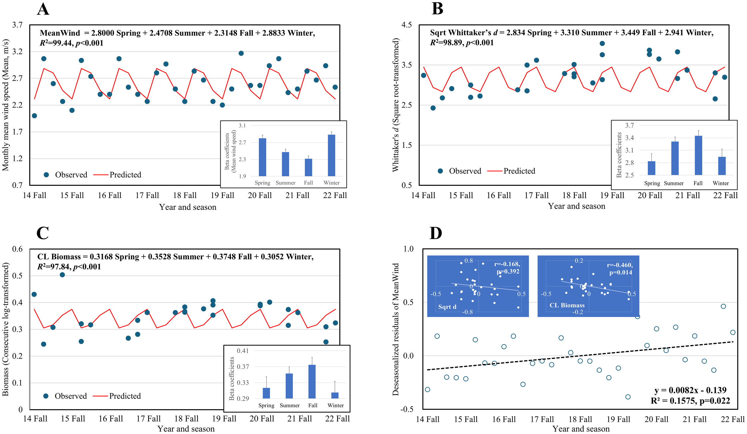
Seasonal mean model analysis showing the seasonal variation of MeanWind (A), macrobenthic diversity, Sqrt d(B), biomass, CL Biomass (C), and a trend fitted on the deseasonalized residuals of MeanWind (D). Inset figures in (A–C) are beta estimates of the seasonal mean model, while those in D are residual plots and correlations between MeanWind and biological parameters, Sqrt d and CL biomass.
Sqrt d was fitted to a seasonal model with R² = 98.89% (p< 0.001), showing increased diversity in the summer and fall (Figure 8B). A minimum beta estimate of Sqrt d of 2.834 was observed in the spring, corresponding to 8.0, which was higher than the diversity anomaly. The CL biomass showed a similar seasonal pattern (R² = 98.89%, p< 0.001) with a minimum beta estimate of 0.3052 in winter, corresponding to 8.9 g/m², which was lower than the biomass anomaly (Figure 8C). The deseasonalized residuals of MeanWind showed a significant positive trend (p = 0.022), negatively correlating with the CL biomass residuals (r = -0.46, p = 0.014), highlighting a difference from Sqrt d, however, with no significant relationship (Figure 8D).
3.6 Prediction of anomaly rounds
Figure 9A shows a comparison of the proportions of anomalous samples in a survey round between Sqrt d and CL biomass. The mean and median proportions of anomalies for Sqrt d (22.7% and 16.7%, respectively) were lower than those for the CL biomass (29.3% and 23.3%, respectively). However, Levene’s and t-test results confirmed that the differences in variances and means were insignificant (p = 0.204 and 0.224, respectively). Figure 9B illustrates a significant linear relationship between the proportions of both parameters, with R2 = 0.7201 (p< 0.001). The covarying patterns of anomalous samples in diversity and biomass suggested a shared disturbance source.
Figure 9
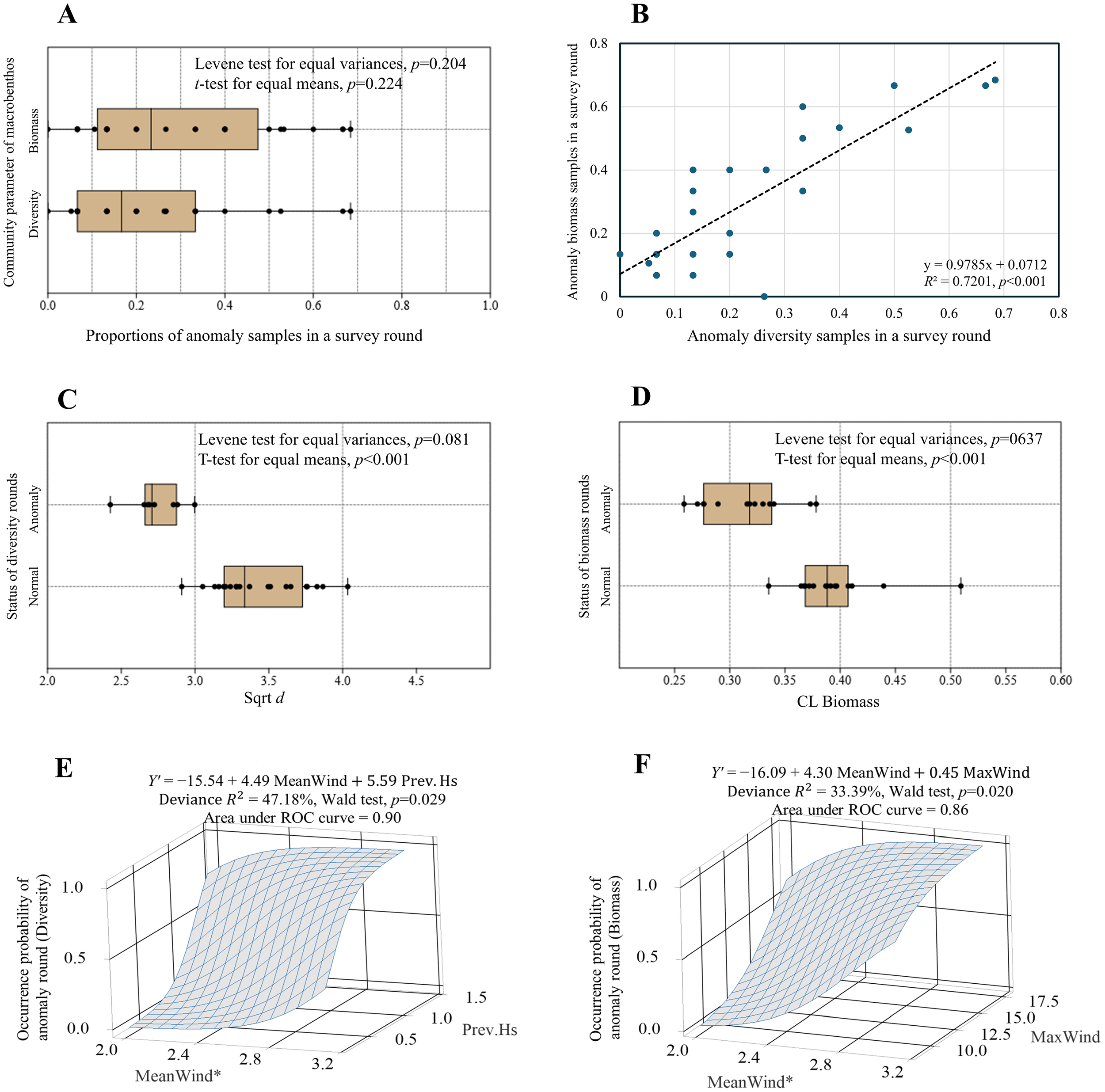
Spear style boxplot depicting the proportions of anomaly samples in a survey round between Sqrt d and CL biomass (A). The linear relationship between the proportions of diversity and biomass (B). Boxplots of Sqrt d and CL biomass between normal and anomaly rounds (C, D). Logistic regression models fitted on the classes of normal (0) and anomaly rounds (1) for diversity and biomass (E, F). The occurrence probability in z-axis was calculated using the equation P(1) = exp(Y’)/(1+exp(Y’)). The symbol * in the x-axis label denotes a p-value less than 0.05.
Figure 9C illustrates the variation in Sqrt d between normal and anomalous rounds. The variances between the groups were equal (standard deviation, 0.31 vs. 0.17; Levene test, p = 0.081) but the means were significantly different (3.43 vs. 2.74; t-test, p< 0.001). The variances in the CL biomass between normal and anomalous rounds were also equal (standard deviation, 0.040 vs. 0.038; Levene’s test, p = 0.637), yet the means were significantly disparate (0.371 vs. 0.321; t-test, p< 0.001) (Figure 9D).
We constructed logistic models to predict the probability of an anomaly round based on air predictors. The final models were selected using a stepwise procedure and Wald tests. The three-dimensional wireframe surface plots for the occurrence probabilities predicted by the significant models are shown in (Figures 9E, F). The deviation R2 values were 47.18% and 33.39% for the diversity and biomass models, respectively. The Wald tests confirmed the significance of the beta values of the model equations (p = 0.029 and 0.020). The AUC values, representing the overall performance of the binary classification model, were satisfactory (AUC = 0.90 and 0.86).
The occurrence probability of a diversity anomaly round increased with MeanWind (p< 0.05) and Prev.Hs (p > 0.05). When Prev.Hs was close to 0.5 m, a MeanWind close to 2.84 m/s could induce a diversity anomaly round, while when Prev.Hs exceeded 1.5 m, a MeanWind >1.59 m/s was required to ensure a diversity anomaly round (Figure 9E). The probability of a biomass anomaly round exhibited a trend similar to that of a diversity anomaly, increasing with MeanWind (p< 0.05) and MaxWind (p > 0.05). When MaxWind was as low as 10 m/s, a MeanWind >2.70 m/s could induce a biomass anomaly round. When MaxWind reached 18 m/s, a MeanWind >1.86 m/s could cause a biomass anomaly round (Figure 9F).
4 Discussion
4.1 Validation
To understand the variation in macrobenthic community parameters, we selected a model from all possible 2k subset regression models using k predictors by means of general model selection criteria, such as Mallows’ Cp, R2, and predicted-R2. We accordingly found that macrobenthic community diversity and biomass had a multifactorial relationship with these predictors. The weather-related predictor variables (e.g., wind speed and significant wave height) used in this study have not been previously used to subtidal macrobenthic communities. Most variations in macrobenthic distribution, diversity, and biomass have been explained by salinity, depth, temperature, organic matter, current, sediment properties, larval supply, and biological interactions (Reise, 1985; Chardy and Clavier, 1988; Snelgrove and Butman, 1994; Snelgrove et al., 1997; Ysebaert et al., 2003; Nilsen et al., 2006; Golubkov, 2008; Fuhrmann et al., 2015). In addition to insufficient background information regarding unfamiliar variables, as recommended by Heinze et al. (2018) and Chen (2022), correlation and regression analyses are statistical methods for analyzing data containing errors. Hence, the results obtained using these methods must be rigorously validated.
The main interest of researchers in field survey studies utilizing empirical models such as ours is to find causally related factors (Reed and Slade, 2008). For a given confined length of data and selected variable subsets from a large number of environmental variables, the unbiasedness of the regression coefficients of predictors may be compromised, resulting in spurious relationships (Sparks and Tryjanowski, 2010; Heinze et al., 2018). As such, we must review whether the estimated regression equation is a realization of the correct source-response relationship, whether it is a result of subset selection from a simple correlation, or whether it is a regression model with biased coefficients (George, 2000; Heinze et al., 2018; Chen, 2022).
Therefore, we believe that issues, such as model robustness or coefficient instability, which determine the reliability of the regression model, deserve examination in this study. According to Kessler et al. (2017), high VIFs are linked to extreme coefficient instability; accordingly, the low VIFs in our study indicated the low coefficient instability of regression models. Bootstrap resampling is a valuable approach for quantifying model stability according to Heinze et al. (2018). However, in its absence, examining the changes in the size and signs of the regression coefficients of the same predictors across models becomes meaningful. Moreover, assessing the predictor inclusion frequencies between different subsets within the same dataset is important for evaluating the unbiasedness or stability of regression model estimates.
The significant regression coefficients of characteristic predictors (e.g., log-transformed sand, depth, and salinity for the diversity model; SPM, copper, and salinity for the biomass model) showed consistent signs across the models, with the exception of DO, which was removed from the air–sea predictor-based model because of its high correlation with other variables. Weather-related predictors also showed negative signs in the regression model, which was consistent with the correlation coefficients presented in Figures 6A, B and 7A, B. Significant predictors such as DO in the diversity model and monthly averages of wind speed (hereafter referred to as wind speed) in the biomass model were estimated to have negative signs. This reflected the relationship between diversity and biomass, which was characterized by a seasonal pattern of higher values in summer and fall, whereas showed an inverse pattern for those of predictors. The relationships predicted by the regression models were also consistent with the seasonality independently estimated from the seasonal mean models.
The inclusion frequencies of the selected predictors across subsets were significantly different from those of the unselected predictors. For example, in the sea predictor-based diversity regression analysis, the inclusion frequencies of log-transformed sand, depth, and salinity were 76–97%, whereas those of unselected predictors varied at 10–76% (no. of subsets, n = 21). In the air–sea predictor-based regression, the same predictors had inclusion frequencies of 83–97%. In addition, the newly included air-related predictor, wind speed, demonstrated a high inclusion frequency of 83%, with those of the remaining predictors ranging from 7% to 69% (n = 29). In the sea predictor-based biomass regression model, the predictors estimated to have the most significant effects (i.e., SPM and sediment Cu) had inclusion frequencies of 95% and 84%, respectively, whereas the unselected predictors had frequencies of 11–79% (n = 19). The same predictors were also included in the air–sea predictor-based regression model, with inclusion frequencies of 96% and 85%, respectively, while the added air predictor, wind speed, had an inclusion frequency of 93%. In contrast, the frequency of unselected predictors in this model ranged from 7% to 78% (n = 27).
Thus, regression coefficient signs and predicted biological parameter responses among the different models showed consistency, which allowed us to evaluate the overall model stability as positive. High inclusion frequencies also suggested that these predictors have high explanatory power, majorly contributing to the improvement in model prediction performance (Heinze et al., 2018). The use of predictor inclusion frequency seems appropriate according to the concept of Granger Causality, which says that variable X “Granger-causes” Y if the predictability of Y declines when X is removed from all possible causative variables, U (Sugihara et al., 2012). In addition, we selected models with the highest predicted R2 and a set of predictors with the highest inclusion frequencies.
Based on the assumption of linearity and additivity, which suggests that the effects of predictors can be additive, the significance of the weather-related predictors as additional explanatory variables and a modest increase in r between sea predictor- and air–sea predictor-based regression can be considered a significant improvement, resulting in a better model (Sparks and Tryjanowski, 2010; Heinze et al., 2018). Therefore, in contrast to previous studies, our findings can be considered a basis for concluding that air predictors have significant explanatory power for variations in biological parameters.
4.2 Ecological significance of the observed relationships
The underlying causes of the observed characteristics are challenging to ascertain using a field survey approach without conducting experiments. In this context, the acquisition of biological knowledge must be prioritized to elucidate the mechanisms responsible for the observed biological responses. This knowledge is instrumental in selecting variables and interpreting models (Sparks and Tryjanowski, 2010). To address this, we examined the significance of the relationships between predictors and biological parameters from an ecological perspective. We believe that this approach allowed us to distinguish between relationships that are correlative or causal.
In this study, the known controllers of macrobenthic diversity and biomass (Section 4.1) were not significantly different from the selected sea predictors; however, some of them (e.g., mean sediment grain size and salinity) showed different or opposite directions from the existing relationships. Regarding the grain size effects of a unimodal pattern on biodiversity in Korean tidal flats at a nationwide spatial scale, Yoo et al. (2013) demonstrated a peak of diversity at 4ϕ in the range of -2–9ϕ, with a decrease in both directions. Thus, the linear relationship between log-transformed sand and diversity in this study did not contradict the previous relationship, considering that the mean grain size in this study ranged from 4 to 7ϕ.
Salinity, traditionally known to have a positive causal relationship with diversity and biomass (Ysebaert et al., 2003), showed a negative correlation in this study. The 95% prediction interval range of the salinity data used in this study was 28–34 psu. This was more limited than the 68% salinity range (14–34 psu) reported by Yoo et al. (2013), which showed a positive effect. The negative effect observed in this study was likely attributed to the restricted data range. Given that much of the temporal variation in biological parameters is seasonal, the negative effect on both parameters reflected an effect similar to that of predictors such as DO, in that lower salinity was also observed in summer and fall. Thus, it can be considered seasonal and correlative rather than a causal relationship. This is supported by the fact that the salinity effect was stronger in the predictions of the average parameters when the spatial variation was removed.
The occurrence and sinking of SPM cause mortality of benthic fauna and severe loss of diversity and biomass through blanketing and resuspension (Clark, 2001; Yoo et al., 2018). Görlich et al. (1987) reported macrobenthic biomass variation from<1 to ~180 g/m2 as a function of SPM, ranging from 10–15 to >1000 mg/L, in the Hornsund Fjord, Spitsbergen, Norway, independent of depth and bottom sediment properties. On the west coast of Korea, locally high concentrations of SPM are responsible for significantly lower species richness, density, and biomass in mudflats and subtidal areas (MLTM, 2009). A neural network simulation estimated that an increase in SPM from 5 to 70 mg/L resulted in a 13% decrease in macrobenthic diversity and >90% decrease in biomass in mudflats when environmental factors other than SPM were fixed at mean values (Yoo et al., 2013; unpublished data for biomass simulation). In the Southeastern Yellow Sea mud (SEYSM), in the southern part of the study area, the benthic habitat quality index, ISEP (Yoo et al., 2010) fluctuated owing to the wide seasonal range of bottom SPM (6.1–845.1 mg/L), with a high SPM value leading to a low-quality status. Yoo et al. (2022) reported that SPM is one of the primary influential factors determining benthic habitat quality on the west coast. The bottom SPM observed in this study ranged from 2.2 to 410.5 mg/L, which is a narrower range of variation than that of the SEYSM. However, this range was sufficiently effective to cause variations in both parameters, based on the simulation results mentioned above. The significance of SPM in explaining the variability of biological parameters reflected the adequacy of the predictor selection and model estimation.
The species-abundance-biomass (SAB) diagram by Pearson and Rosenberg (1978) shows that the response of each SAB parameter to a stressor can vary according to stress intensity. In this study, beta estimates from seasonality analysis were converted to anti-log diversity and biomass, and the maximum/minimum ratio for each parameter was calculated. This ratio was 68% for diversity (Whittaker’s d, spring = 8.03 and fall = 11.90) and 42% for biomass (wet weight, winter = 9.45 and fall = 22.46 g/m2), respectively. According to these ratios, biomass had a relatively larger seasonal variation range than diversity, with the winter beta estimate of biomass being close to the biomass anomaly of 9.10 g/m2, whereas the spring beta estimate of diversity was higher than the diversity anomaly of 6.6. As the impact of SPM mentioned above was greater for biomass than for diversity, a potential disturbance agent with seasonality might have exerted a greater effect on biomass.
The symmetrical seasonality between the biological parameters and wind speed (Figure 8) suggested that both diversity and biomass were affected by wind speed or other covariates with similar seasonal patterns. The deseasonalized residuals of wind speed showed a linearly increasing trend. However, the residuals of diversity were independent of the deseasonalized residuals of wind speed, whereas those of biomass showed a significant negative correlation. Independent estimation of seasonal patterns for the two variables may match; however, if the deseasonalized residuals of both are uncorrelated, this may suggest (1) a lack of a bidirectional or unidirectional relationship between them (Sugihara et al., 2012) or (2) different ecological characteristics, such as different sensitivities to specific disturbances (Dong et al., 2021). In contrast to the survey-averaged diversity model (Figure 7 and Table 3), in which it was removed because of its high correlation with DO, wind speed had a more pronounced effect on the survey-averaged biomass model. The proportion of total variance (R²) in biomass explained solely by wind speed was greater than 50%, based on the one-to-one relationship between wind speed and biomass (r = 0.71, p< 0.001; Figure 7B). A relatively low correlation does not necessarily indicate lack of causation. Despite the observed disparate response levels, wind speed may serve as a proximate cause for both parameters. KOWP (2015) argued that wind in the study area is a potential factor for sediment disturbance. A detailed description of the possible reasons for this factor to be more closely related to biomass is provided in Section 4.3.
4.3 Impact of wind on coastal macrobenthic communities
Low wind speeds have been identified as a possible cause of coral bleaching, because they favor localized heating and high penetration of solar radiation (Glynn, 1993). However, wind speed affects pelagic ecosystems in the following ways. (1) Wind generates upward transport of nutrients from deep waters, promoting primary production, and affects the whole ecosystem globally and at all scales from plankton to birds and mammals (Sakshaug et al., 2000). (2) High wind speeds suppress bloom occurrence by altering water column stability and creating a shallower mixed layer, particularly due to melting ice and the associated release of iron in the marginal ice zone of the Southern Ocean (Fitch and Moore, 2007). (3) Wind-driven turbulent mixing during the spawning season hinders the generation of sufficient food concentrations, affecting the survival variability of young fish larvae more than cannibalism or offshore transport (Peterman and Bradford, 1987).
The use of hydrodynamic and climatic variables as predictors of macrobenthic community parameters is common in intertidal and adjacent shallow zones. Ricciardi and Bourget (1999) predicted the global patterns of macrobenthos biomass in sedimentary shores using variables such as the mean wave height, intertidal slope, and wave exposure and found that wave exposure had a significant negative effect, attributed to the susceptibility of soft bottom fauna to wave stress. Comparing macrobenthic communities in diverse types of sandy beaches, from reflective to dissipative and tidal flats, in the order of diminishing physical control, revealed that diversity and biomass increased with decreasing wave energy (Brown and McLachlan, 1990; Defeo and McLachlan, 2005). Paavo et al. (2011) and Armonies et al. (2014) showed that, on sandy coasts, these wave-related processes that determine community shape extended into shallow subtidal areas in the ~30 m depth range, resulting in increased macrobenthic species richness and abundance as wave-induced turbulence and sediment instability decreased, followed by their stabilization at depths where the processes were not effective.
The study area, an open coast with exposed shorelines and a sheltered bay, experiences tidal mixing across all water bodies due to strong tidal currents, even in summer when stratification can develop (Baek and Moon, 2019). The Geum River estuary, Saemangeum reclaimed land, and Gunjang National Industrial Complex, located approximately 50 km north of the wind farm, are potential sources of pollution. The annual average DO on the Gunsan coast has been neutral since the 80s, while the COD has averaged at approximately 2 mg/L since the 70s. The annual averages of DIN (0.114 mg/L) and phosphate (0.014 mg/L) in Gomso Bay, which is on the eastern side of the study area, were significantly lower than those on the western and southern coasts of Korea (Park et al., 2009). Recently, there have been concerns raised about the potential risks to human health due to the release of heavy metals from OWFs, which may lead to changes in the benthic microbial community and accumulation in seafood (Wang et al., 2023; Watson et al., 2025). The water quality of the study area was generally good, and moderate or lower environmental quality status in the study area was observed at a very low frequency. Vigilant monitoring for heavy metals is necessary, however, as previously mentioned, the maximum concentration of copper in the study area was below the ERL, as with other heavy metals (see environmental descriptions in Section 2.1).We inferred that sediment Cu and DO, which were selected as effective predictors, were correlative agents (e.g., mean sediment grain size and organic matter content for Cu; temperature for DO), rather than being pollution-related.
On the south coast, with its complex coastline and bays, the recurring marked seasonality is caused by a hypoxia-induced decline in SAB parameters (Seo et al., 2015). Seasonality, driven by the emergence of poor macrobenthic assemblages, is associated with regression/recovery patterns attributed to the presence of disturbance sources (Froehlich et al., 2015; Magni et al., 2015). Although natural variability in food availability and reproduction/recruitment is an important component of seasonality, interannual variability is often more pronounced in pristine areas (Nasi et al., 2017). Despite its generally good status, the macrobenthic biomass in this area is lower in winter than that in other areas on the west coast of Korea, a characteristic feature of seasonality (Jeong et al., 2019). Currently, on the west coast of Korea, relatively poor assemblages caused by natural disturbance agents are mainly observed during the summer monsoon in tidal flats due to heavy rainfall, and in subtidal areas due to oceanic floods (Wheatcroft, 2000), indicating the impact of buried sediments from rivers on coastal benthic ecosystems in summer (Hong and Yoo, 1996; Yoo and Hong, 1996; Yoo et al., 2016).
Frequent storm surges and extremely heavy snow under high-energy states occur extensively on the west coast of Korea during winter owing to northwesterly winds (Chong and Seol, 2007). The monthly average of storm days with wind speeds greater than 13.9 m/s is ≥3 d in winter and<1 d in summer (Cho et al., 2001). Significant wave heights of >4 m were reported in the study area during the winter of 2014-15. This was likely the cause of the massive burial of 1–2 m in thickness, as measured by pressure sensor data obtained after the acoustic Doppler current profiler (ADCP) was buried and recovered (KOWP, 2015). The event suggested that sediment deposition at scales larger than those of oceanic floods (e.g., ~10 cm thick; Thrush et al., 2003), occurs due to winter storms, affecting the benthic communities in the study area. The overall significant negative correlations between the weather-related predictors and biological parameters, the relatively strong wind speeds in winter and spring, and the sedimentation events due to winter storms in the study area could indicate that weather and related wave conditions influence the benthic ecosystem and are responsible for the differences in the seasonality of macrobenthic community parameters compared with that in other parts of the west coast.
Despite the dominance of northwesterly winds along the entire west coast, wind speed was responsible for the (1) negative effect on macrobenthic community parameters, (2) unusual occurrence of biomass anomalies in the study area, and (3) seasonality, which was contradictory to that of other areas. Which are the reasons for wind triggering an ecological response that was only prominent in this region, and for the limited influence of the Hs/depth ratio, which reflects the depth effect and is applicable to wide depth ranges, compared with that of other weather-related predictors? Wind-generated waves strongly influence sediment erosion or stability, and one of the variables that characterize waves is depth (Nelson and Fringer, 2018). The spatial confinement of the wind effect and neutralization of the Hs/depth ratio effect are apparently attributed to the shallow and relatively narrow depth range of the study area (see environmental descriptions in Section 2.1). In our previous study (Yoo, unpublished data) conducted on a larger spatial scale with a different depth range, the explanatory power of the Hs/depth ratio was significant; therefore, the effectiveness of this variable should be further tested.
The predictions of our study based on observations from weather stations close to the shore are not applicable to other areas. In our study, offshore measurements from CWBs, such as offshore wind speed and significant wave height, were unrelated to biological parameters; the underlying reasons for this remain unclear. The measurement conditions of land weather stations vary considerably according to factors such as altitude, topography, and distance from shore. Hence, the data from several nearby land and offshore weather stations must be collected and compared prior to making any predictions. The effects of wind speed are unlikely to reach the deep seafloor beyond the shallow area; therefore, estimates such as the anomaly occurrence threshold ranges for diversity and biomass are probably limited to our study domain.
Given the different phenomenon of soft-bottom macroinvertebrate diversity increase and biomass decrease at the southeastern part of wind turbine foundations in an OWF in Pinghai Bay, China (Lu et al., 2020), a careful approach for the generalization of the observed patterns in the study area are required. As previously described, we did not use an experimental approach to demonstrate whether air predictors have a causal effect. An empirical analysis could be conducted to test the statistical differences in community parameters between the areas divided by considering the dominant wind power, wind frequency or spatial projection from wind-wave model. To demonstrate a cause of biomass increase/decrease, it is important to determine where reef effect or wind-induced sediment disturbance prevails through a coupled approach of natural experiment and trophic modeling. For the former effect, Wang et al. (2019) used energy flow model to prove that increased organic matter resulting in increased anchovies and some benthic fish biomass. At present, capturing the exact timing, possible lagged response, or persistence of an anomalous event is difficult due to the irregular surveys. Despite these caveats, our results highlight the need to use a range of air predictors, including wind speed, as potential causative agents to explain the variations in macrobenthic communities in coastal waters. Furthermore, they suggest that strategically located land-based weather stations near coastlines can be effective in predicting the rich or poor status of macrobenthic production.
Which are the reasons for wind affecting biomass variation more, or for having a differential effect between the two parameters? The recovery time after mass mortality of marine benthic communities due to catastrophic disturbances varies from a few days to several months and years, depending on the biota (e.g., diatoms, nematodes, and macrobenthos), body size, and life strategy (Odum, 1969; Dittmann et al., 1999). Low diversity and reduced mean body size, biomass, and productivity are typically observed when sediment disturbances occur (Thrush et al., 2003). In this process, biomass recovery takes longer (weeks or months vs. years) than numerical recoveries, such as those of diversity and abundance (Beukema et al., 1999).
It is a common understanding in ecology that the significant contribution of large-bodied organisms, which have a slow growth, to the macrobenthic biomass is responsible for the extended recovery time for reaching the same levels as those of the predisturbance and unaffected ambient levels of biomass. For example, the species with the highest contribution in terms of macrobenthic biomass in this study was the heart urchin, Echinocardium cordatum (9% frequency, and 26% of total biomass), and the species’ per capita wet weight reached 32.9 g. Nakamura (2001) reported that the species became 120 mg ash free dry weight at the third year (5.2 g in wet weight by multiplying conversion ratio, 43.5 for Irregularia, Echinoidea; Dr. Thomas Brey, http://www.thomas-brey.de/science/virtualhandbook/navlog/index.html). Opportunistic species including Capitellidae, Spionidae and Cirratulidae polychaetes dominated abundance during most of the study period. These opportunistic species took only a few tens of days to go from zero to peak abundance, and within about 200 days the community structure and composition became similar (Rhoads et al., 1978; Hashimoto and Sato-Okoshi, 2022). This type of recovery may cause increased seasonal variation as described above or lead to a more pronounced response than that of diversity. Moreover, biomass anomaly/recovery could lead to the declining production of higher trophic levels, suggesting that climatic variables should also be considered as potential factors regulating fishery stocks in coastal areas.
Our study provides further insights into the potential wind mechanisms that control diversity and biomass variation in coastal areas. Since the 1970s, a phenomenon known as global stilling has been observed, which refers to decreasing trends in global wind speeds over several decades (Azorin-Molina et al., 2017). Nevertheless, increasing trends in wind speed and wave height have also been reported recently (Young et al., 2011; Zheng et al., 2016, Zheng et al., 2022). We observed an increasing trend in wind speed in the study area over a short period of approximately a decade. If the increase in wind speed in the area is consistent with the global trend and continues to be so, the decline in macrobenthic biomass production may also continue, even in the absence of negative effects of pollution or construction/operation of wind farm structures.
Wind farms and other marine facilities, such as wave energy converters, fish cages, and even seaweed production areas, influence waves and current fields, and thus sediment transport and shoreline development (Christensen et al., 2014). Based on modeling, wind farms can affect the energy transfer from wind to waves, as follows: (1) the significant wave height Hs is reduced by up to ~5% close to a wind farm, (2) the wave energy is reduced by up to 10% on the lee side of a wind farm, (3) the area with an Hs reduction of >1% can reach 15–888 km2, and (4) the effect of wind farms on waves can results in shoreline progression of 30 m/100 years for 10 km from the lee side (Christensen et al., 2013, 2014; Fischereit et al., 2022). Wave attenuators or energy converters that shield aquaculture facilities or habitats from wave disturbances contribute to increased offshore fish production and promote vegetation growth, improving the supply of ecosystem services (Silva et al., 2018; Sreeranga et al., 2021).
Wave attenuators may have ecologically detrimental effects such as trapping sediment between the shore and attenuator (Rheinhardt and Brinson, 2007). Studies on offshore wind energy installations in the North Sea reported that anthropogenic structures have caused a significant increase in macrobenthic diversity and abundance on a large scale. In the wake of the turbine foundations of OWFs, hydrodynamic changes from reduced tidal currents lead to finer sediment grain sizes and increased sediment organic matter. Environmental changes are further complemented by the contribution of organic matter input from the sedimentation of feces and detritus produced by hard substrate epifauna and by the foundation effects creating sheltered habitats and enhancing larval settlement, resulting in the enrichment of abundance and biomass of macrobenthic communities (Maar et al., 2009; Coates et al., 2014). In a high wave-energy environment, the expansion of OWFs can act as a driver of positive changes in the ecosystem, including an increase in macrobenthic and fisheries production. Owing to intermittent monitoring and a lack of consistent survey data, we were unable to validate the wake effect in our study. We recommend a long-term natural experimental approach to validate the effect of OWFs on macrobenthic communities in the future.
Statements
Data availability statement
The raw data supporting the conclusions of this article will be made available by the authors, without undue reservation.
Ethics statement
The manuscript presents research on animals that do not require ethical approval for their study.
Author contributions
SJ: Formal Analysis, Writing – original draft, Writing – review & editing. SO: Project administration, Writing – review & editing. SK: Formal Analysis, Investigation, Writing – original draft. CL: Data curation, Investigation, Writing – original draft. DA: Data curation, Investigation, Writing – original draft. CK: Investigation, Methodology, Writing – review & editing. DL: Data curation, Visualization, Writing – original draft. JY: Conceptualization, Supervision, Writing – original draft, Writing – review & editing.
Funding
The author(s) declare financial support was received for the research and/or publication of this article. This research was supported by grants from the research project “Environmental Impact Analysis on Offshore Wind Farm and Database System Development”, which was driven by the Korea Environment Institute (KEI) and funded by the Korea Institute of Energy Technology Evaluation and Planning (KETEP) and the Ministry of Trade, Industry, and Energy (MOTIE) of Korea (Project Nos. 20203030020080 and PN91870).
Conflict of interest
The authors declare that the research was conducted in the absence of any commercial or financial relationships that could be construed as a potential conflict of interest.
Generative AI statement
The author(s) declare that no Generative AI was used in the creation of this manuscript.
Any alternative text (alt text) provided alongside figures in this article has been generated by Frontiers with the support of artificial intelligence and reasonable efforts have been made to ensure accuracy, including review by the authors wherever possible. If you identify any issues, please contact us.
Publisher’s note
All claims expressed in this article are solely those of the authors and do not necessarily represent those of their affiliated organizations, or those of the publisher, the editors and the reviewers. Any product that may be evaluated in this article, or claim that may be made by its manufacturer, is not guaranteed or endorsed by the publisher.
References
1
Armonies W. Buschbaum C. Hellwig-Armonies M. (2014). The seaward limit of wave effects on coastal macrobenthos. Helgol. Mar. Res.68, 1–16. doi: 10.1007/s10152-013-0364-1
2
Azorin-Molina C. Vicente-Serrano S. M. McVicar T. R. Revuelto J. Jerez S. López-Moreno J. I. (2017). Assessing the impact of measurement time interval when calculating wind speed means and trends under the stilling phenomenon. Int. J. Climatol.37, 480–492. doi: 10.1002/joc.4720
3
Baek Y. H. Moon I. J. (2019). The accuracy of satellite-composite GHRSST and model-reanalysis sea surface temperature data at the seas adjacent to the Korean Peninsula. Ocean Polar Res.41, 213–232. doi: 10.4217/OPR.2019.41.4.213
4
Bergström L. Kautsky L. Malm T. Rosenberg R. Wahlberg M. Capetillo N. et al . (2014). Effects of offshore wind farms on marine wildlife—a generalized impact assessment. Environ. Res. Lett.9, 34012. doi: 10.1088/1748-9326/9/3/034012
5
Beukema J. J. Flach E. C. Dekker R. Starink M. (1999). A long-term study of the recovery of the macrozoobenthos on large defaunated plots on a tidal flat in the Wadden Sea. J. Sea Res.42, 235–254. doi: 10.1016/S1385-1101(99)00027-1
6
Bradshaw A. D. (2002). “Introduction and philosophy,” in Handbook of Ecological Restoration, 1 Principles of Restoration. Eds. PerrowM. R.DavyA. J. (Cambridge: Cambridge University Press), 3–9. doi: 10.1016/j.ecoleng.2004.02.001
7
Brey T. (2012). A multi-parameter artificial neural network model to estimate macrobenthic invertebrate productivity and production. Limnol. Oceanogr. Methods10, 581–589. doi: 10.4319/lom.2012.10.581
8
Brown A. C. McLachlan A. (1990). Ecology of Sandy Shores (Amsterdam: Elsevier).
9
Chardy P. Clavier J. (1988). Biomass and trophic structure of the macrobenthos in the south-west lagoon of New Caledonia. Mar. Biol.99, 195–202. doi: 10.1007/BF00391981
10
Chen J. Pillai A. C. Johanning L. Ashton I. (2021). Using machine learning to derive spatial wave data: A case study for a marine energy site. Environ. Modell. Software142, 105066. doi: 10.1016/j.envsoft.2021.105066
11
Chen X. (2022). “Confirmation with multiple regression analysis,” in Quantitative Epidemiology, (Emerging topics in statistics and biostatics (Springer, Cham), 125–162. doi: 10.1007/978-3-030-83852-2_5
12
Cho Y. S. Lee W. C. Kim J. B. Hong S. J. Kim H. C. Kim C. S. (2013). Establishment of environmental assessment using sediment total organic carbon and macrobenthic polychaete community in shellfish farms. J. Korean Soc Mar. Environ. Saf.19, 430–438. doi: 10.7837/kosomes.2013.19.5.430
13
Cho Y. G. Lee C. B. Park Y. A. Kim D. C. Kang H. J. (1993). Geochemical Characteristics of surface sediments in the eastern part of the Yellow Sea and the Korean west coast. Korean J. Quat. Res.7, 69–91.
14
Cho J. W. Lim D. I. Kim B. O. (2001). Observation of shoreline change using an aerial photograph in Hampyung Bay, southwestern coast of Korea. J. Korean Earth Sci. Soc22, 317–326.
15
Choi B. S. (1992). Univariate Time Series Analysis 1 (Seoul: Sekyungsa), 736.
16
Choi K. (2014). Morphology, sedimentology and stratigraphy of Korean tidal flats–Implications for future coastal managements. Ocean Coast. Manage.102, 437–448. doi: 10.1016/j.ocecoaman.2014.07.009
17
Choi J. K. Shim J. H. (1986). The ecological study of phytoplankton in Kyeonggi Bay, Yellow Sea: II. Light intensity, transparency, suspended substances. J. Oceanogr. Soc Korea.21, 101–109.
18
Chong K. C. Seol D. I. (2007). A selection of the refuge area in the west sea for the national fishery supervision vessel according to the trajectories of the extratropical cyclone in winter season. J. Navig. Port Res.31, 555–562. doi: 10.5394/KINPR.2007.31.6.555
19
Christensen E. D. Johnson M. Sørensen O. R. Hasager C. B. Badger M. Larsen S. E. (2013). Transmission of wave energy through an offshore wind turbine farm. Coast. Eng.82, 25–46. doi: 10.1016/j.coastaleng.2013.08.004
20
Christensen E. D. Kristensen S. E. Deigaard R. (2014). Impact of an offshore wind farm on wave conditions and shoreline development. Coast. Eng.34. doi: 10.9753/icce.v34.sediment.87
21
Clark R. B. (2001). Marine Pollution-Fifth Edition (Oxford: Oxford University Press), 237.
22
Coates D. A. Deschutter Y. Vincx M. Vanaverbeke J. (2014). Enrichment and shifts in macrobenthic assemblages in an offshore wind farm area in the Belgian part of the North Sea. Mar. Environ. Res.95, 1–12. doi: 10.1016/j.marenvres.2013.12.008
23
Coosen J. Seys J. Meire P. M. Craeymeersch J. A. M. (1994). Effect of sedimentological and hydrodynamical changes in the intertidal areas of the Oosterschelde estuary (SW Netherlands) on distribution, density and biomass of five common macrobenthic species: Spio martinensis (Mesnil), Hydrobia ulvae (Pennant), Arenicola marina (L.), Scoloplos armiger (Muller) and Bathyporeia sp. Hydrobiologia.282, 235–249. doi: 10.1007/BF00024633
24
Defeo O. McLachlan A. (2005). Patterns, processes and regulatory mechanisms in sandy beach macrofauna: a multi-scale analysis. Mar. Ecol. Prog. Ser.295, 1–20. doi: 10.3354/meps295001
25
Dittmann S. Günther C.-P. Schleier U. (1999). “Recolonization of tidal flats after disturbance,” in The Wadden Sea Ecosystem: Stability, Problems and Mechanisms. Ed. DittmannS. (Springer, Berlin and Heidelberg), 175–192. doi: 10.1007/978-3-642-60097-5_6
26
Donadi S. Eriksson B. K. Lettmann K. A. Hodapp D. Wolff J. O. Hillebrand H. (2015). The body-size structure of macrobenthos changes predictably along gradients of hydrodynamic stress and organic enrichment. Mar. Biol.162, 675–685. doi: 10.1007/s00227-015-2614-z
27
Dong J. Y. Zhao L. Yang X. Sun X. Zhang X. (2021). Functional trait responses of macrobenthos to anthropogenic pressure in three temperate intertidal communities. Front. Mar. Sci.8. doi: 10.3389/fmars.2021.756814
28
Ferguson C. A. Carvalho L. Scott E. M. Bowman A. W. Kirika A. (2008). Assessing ecological responses to environmental change using statistical models. J. Appl. Ecol.45, 193–203. doi: 10.1111/j.1365-2664.2007.01428.x
29
Fischereit J. Larsén X. G. Hahmann A. N. (2022). Climatic impacts of wind-wave-wake interactions in offshore wind farms. Front. Energy Res.10. doi: 10.3389/fenrg.2022.881459
30
Fitch D. T. Moore J. K. (2007). Wind speed influence on phytoplankton bloom dynamics in the Southern Ocean Marginal Ice Zone. J. Geophys. Res. Oceans112, C08006. doi: 10.1029/2006JC004061
31
Folk R. L. Ward W. C. (1957). Brazos River bar: a study in the significance of grain size parameters. J. Sediment. Res.27, 3–26. doi: 10.1306/74d70646-2b21-11d7-8648000102c1865d
32
Frey R. W. Hong J. S. Howard J. D. Park B. K. Han S. J. (1987). Zonation of benthos on a macrotidal flat, Inchon, Korea. Senckenberg. Marit.19, 295–329.
33
Froehlich H. E. Hennessey S. M. Essington T. E. Beaudreau A. H. Levin P. S. (2015). Spatial and temporal variation in nearshore macrofaunal community structure in a seasonally hypoxic estuary. Mar. Ecol. Prog. Ser.520, 67–83. doi: 10.3354/meps11105
34
Fuhrmann M. M. Pedersen T. Ramasco V. Nilssen E. M. (2015). Macrobenthic biomass and production in a heterogenic subarctic fjord after invasion by the red king crab. J. Sea Res.106, 1–13. doi: 10.1016/j.seares.2015.09.003
35
George E. I. (2000). The variable selection problem. J. Am. Stat. Assoc.95, 1304–1308. doi: 10.1080/01621459.2000.10474336
36
Glynn P. W. (1993). Coral reef bleaching: ecological perspectives. Coral Reefs.12, 1–17. doi: 10.1007/BF00303779
37
Golubkov S. (2008). “Factors affecting the role of macrobenthos in pelagic-benthic coupling in the Neva Bay (eastern Gulf of Finland),” in 2008 IEEE/OES US/EU-Baltic International Symposium (IEEE Publications, Tallinn, Estonia), 1–6. doi: 10.1109/BALTIC.2008.4625566
38
Görlich K. Weslawski J. M. Zajaczkowski M. (1987). Suspension settling effect on macrobenthos biomass distribution in the Hornsund fjord, Spitsbergen. Polar Res.5, 175–192. doi: 10.3402/polar.v5i2.6875
39
Ha K. J. Heo K. Y. Lee S. S. Yun K. S. Jhun J. G. (2012). Variability in the East Asian monsoon: a review. Meteorol. Appl.19, 200–215. doi: 10.1002/met.1320
40
Hashimoto A. Sato-Okoshi W. (2022). Population dynamics of Capitella aff. teleta (Polychaeta, Capitellidae) in Gamo Lagoon, northeastern Japan, during a series of restoration works following the 2011 Great East Japan Earthquake and tsunami. Front. Mar. Sci.9. doi: 10.3389/FMARS.2022.1001925/BIBTEX
41
Heinze G. Wallisch C. Dunkler D. (2018). Variable selection–a review and recommendations for the practicing statistician. Biom. J.60, 431–449. doi: 10.1002/bimj.201700067
42
Hiscock K. Tyler-Walters H. Jones H. (2002). High Level Environmental Screening Study for Offshore Wind Farm Developments – Marine Habitats and Species Project (Report from the Marine Biological Association to the Department of Trade and Industry New & Renewable Energy Programme). (AEA Technology, Environment Contract: W/35/00632/00/00.).
43
Hong J. S. Yoo J. W. (1996). Salinity and sediment types as sources of variability in the distribution of the benthic macrofauna in Han Estuary and Kyonggi Bay, Korea. Ocean Sci. J.31, 217–231.
44
Hwang J. H. Van S. P. Choi B. J. Chang Y. S. Kim Y. H. (2014). The physical processes in the Yellow Sea. Ocean Coast. Manage.102, 449–457. doi: 10.1016/j.ocecoaman.2014.03.026
45
Jeong S. Y. Lee C. L. Gim S. H. Kim S. Myoung J. G. Oh S. Y. et al . (2019). Ecological evaluation on the biomass of macrobenthic communities observed from a planned offshore wind farm area, West Coast of Korea. Ocean Polar Res.41, 311–318. doi: 10.4217/OPR.2019.41.4.311
46
Jeong B. G. Shin H. C. (2018). Spatiotemporal variation and evaluation of benthic healthiness of macrobenthic polychaetous community on the Coast of Ulsan. Ocean Polar Res.40, 223–235. doi: 10.4217/OPR.2018.40.4.223
47
Kessler R. C. Stein M. B. Petukhova M. V. Bliese P. Bossarte R. M. Bromet E. J. et al . (2017). Predicting suicides after outpatient mental health visits in the Army Study to Assess Risk and Resilience in Servicemembers (Army STARRS). Mol. Psychiatry22, 544–551. doi: 10.1038/mp.2016.110
48
Kim H. G. Kang Y. H. (2012). The 2010 wind resource map of the Korean Peninsular. J. Wind Eng. Inst. Korea16, 167–172.
49
KOWP (2015). Marine Environment and Ecological Baseline Survey Report for the Southwest Offshore Wind Development Project (Seoul: Korea Offshore Wind Power Co. Ltd), 723.
50
Li C. Coolen J. W. P. Scherer L. Mogollón J. M. Braeckman U. Vanaverbeke J. et al . (2023). Offshore wind energy and marine biodiversity in the North Sea: life cycle impact assessment for benthic communities. Environ. Sci. Technol.57, 6455–6464. doi: 10.1021/acs.est.2c07797
51
Lu Z. Zhan X. Guo Y. Ma L. (2020). Small-scale effects of offshore wind-turbine foundations on macrobenthic assemblages in Pinghai Bay, China. J. Coast. Res.36, 139–147. Available online at: https://www.jstor.org/stable/26864923.
52
Maar M. Bolding K. Petersen J. K. Hansen J. L. S. Timmermann K. (2009). Local effects of blue mussels around turbine foundations in an ecosystem model of Nysted off-shore wind farm, Denmark. J. Sea Res.62, 159–174. doi: 10.1016/j.seares.2009.01.008
53
Magni P. Draredja B. Melouah K. Como S. (2015). Patterns of seasonal variation in lagoonal macrozoobenthic assemblages (Mellah lagoon, Algeria). Mar. Environ. Res.109, 168–176. doi: 10.1016/j.marenvres.2015.07.005
54
Maxwell S. M. Kershaw F. Locke C. C. Conners M. G. Dawson C. Aylesworth S. et al . (2022). Potential impacts of floating wind turbine technology for marine species and habitats. J. Environ. Manag307, 114577. doi: 10.1016/j.jenvman.2022.114577
55
MLTM (2009). National Investigation of Marine Ecosystem-(Southern part of the west coast of Korea, 35.5°N Yeonggwang-34.5°N Jindo) (Gwacheon: Ministry of Land, Transport and Maritime Affairs), 692.
56
Munyati C. Sinthumule N. I. (2021). Comparative suitability of ordinary kriging and Inverse Distance Weighted interpolation for indicating intactness gradients on threatened savannah woodland and forest stands. Environ. Sustain. Indic12, 100151. doi: 10.1016/j.indic.2021.100151
57
Nakamura Y. (2001). Autoecology of the heart urchin, Echinocardium cordatum, in the muddy sediment of the Seto Inland Sea, Japan. J. Mar. Biol. Assoc. United Kingdom81, 289–297. doi: 10.1017/S0025315401003769
58
Nasi F. Auriemma R. Bonsdorff E. Cibic T. Aleffi I. F. Bettoso N. et al . (2017). Biodiversity, feeding habits and reproductive strategies of benthic macrofauna in a protected area of the northern Adriatic Sea: a three-year study. Mediterr. Mar. Sci.18, 292–309. doi: 10.12681/mms.1897
59
Nelson K. S. Fringer O. B. (2018). Sediment dynamics in wind wave-dominated shallow-water environments. J. Geophys. Res. Oceans.123, 6996–7015. doi: 10.1029/2018JC013894
60
Nilsen M. Pedersen T. Nilssen E. M. (2006). Macrobenthic biomass, productivity (P/B) and production in a high-latitude ecosystem, North Norway. Mar. Ecol. Prog. Ser.321, 67–77. doi: 10.3354/meps321067
61
Odum E. P. (1969). The strategy of ecosystem development. Science.164, 262–270. doi: 10.1126/science.164.3877.262
62
Paavo B. Jonker R. Thrush S. Probert P. K. (2011). Macrofaunal community patterns of adjacent coastal sediments with wave-reflecting or wave-dissipating characteristics. J. Coast. Res.27, 515–528. doi: 10.2112/JCOASTRES-D-10-00001.1
63
Paik S. G. Kang R. S. Jeon J. O. Lee J. H. Yun S. G. (2007). Distribution patterns of sandy bottom macrobenthic community on the Hupo coastal area, in the East Sea of Korea. Ocean Polar Res.29, 123–134. doi: 10.4217/OPR.2007.29.2.123
64
Park S. Y. Choi O. I. Kwon J. N. Jeon K. A. Jo J. Y. Kim H. C. et al . (2009). Long-term variation and characteristics of water quality in the Gunsan coastal areas of Yellow Sea, Korea. J. Korean Soc Mar. Environ. Saf.15, 297–313.
65
Park M. O. Lee Y. W. Park J. K. Kang C. S. Kim S. G. Kim S. S. et al . (2019). Evaluation of the seawater quality in the coastal area of Korea in 2013–2017. JKOSMEE.22, 47–56. doi: 10.7846/JKOSMEE.2019.22.1.47
66
Paskyabi M. B. (2015). Offshore wind farm wake effect on stratification and coastal upwelling. Energy Proc.80, 131–140. doi: 10.1016/j.egypro.2015.11.415
67
Pearson T. H. Rosenberg R. (1978). Macrobenthic succession in relation to organic enrichment and pollution of the marine environment. Oceanogr. Mar. Biol. Annu. Rev.16, 229–311.
68
Peterman R. M. Bradford M. J. (1987). Wind speed and mortality rate of a marine fish, the northern anchovy (Engraulis mordax). Science235, 354–356. doi: 10.1126/science.235.4786.354
69
Reed A. W. Slade N. A. (2008). Density-dependent recruitment in grassland small mammals. J. Anim. Ecol.77, 57–65. doi: 10.1111/j.1365-2656.2007.01327.x
70
Reise K. (1985). Tidal Flat Ecology-An Experimental Approach to Species Interaction (Berlin, Heidelberg: Springer-Verlag), 191.
71
Rheinhardt R. D. Brinson M. M. (2007). Framework for Developing a Reference-Based Assessment Approach for Evaluating the Ecological Condition of Coastal Watersheds (Greenville, North Carolina: East Carolina University).
72
Rhoads D. C. McCall P. L. Yingst J. Y. (1978). Disturbance and Production on the Estuarine Seafloor: Dredge-spoil disposal in estuaries such as Long Island Sound can be managed in ways that enhance productivity rather than diminish it. Am. Sci.66, 577–586. Available online at: http://www.jstor.org/stable/27848852 (Accessed June 1, 2025).
73
Ricciardi A. Bourget E. (1999). Global patterns of macroinvertebrate biomass in marine intertidal communities. Mar. Ecol. Prog. Ser.185, 21–35. doi: 10.3354/meps185021
74
Sakshaug E. Tangen K. Slagstad D. (2000). “Marine primary production and the effects of wind,” in The Changing Ocean Carbon Cycle: a Midterm Synthesis of the Joint Global Ocean Flux Study. Eds. DucklowH. W.FieldJ. G. (Cambridge University Press, Hanson: RB), 19–36.
75
Seelam J. K. Baldock T. E. (2012). Measurement and modeling of solitary wave induced bed shear stress over a rough bed, in Proceedings of the Coastal Engineering Conference (Coastal Engineering Research Council), 33. doi: 10.9753/icce.v33.waves.21
76
Seo J. Y. Lim H. S. Choi J. W. (2015). Spatio-temporal distribution of macrobenthic communities in Jinhae Bay, Korea. Ocean Polar Res.37, 295–315. doi: 10.4217/OPR.2015.37.4.295
77
Silva D. Rusu E. Guedes Soares C. G. (2018). The effect of a wave energy farm protecting an aquaculture installation. Energies.11, 2109. doi: 10.3390/en11082109
78
Snelgrove P. V. R. Blackburn T. H. Hutchings P. A. Alongi D. M. Grassle J. F. Hummel H. et al . (1997). The importance of marine sediment biodiversity in ecosystem processes. Ambio.26, 578–584.
79
Snelgrove P. V. R. Butman C. A. (1994). Animal-sediment relationships revisited: cause versus effect. Oceanogr. Lit. Rev.32, 111–177.
80
Sparks T. Tryjanowski P. (2010). “Regression and causality,” in Phenological Research: Methods for Environmental and Climate Change Analysis. Eds. HudsonI. L.KeatleyM. R. (Springer), 123–145.
81
Sreeranga S. Takagi H. Shirai R. (2021). Community-based portable reefs to promote mangrove vegetation growth: bridging between ecological and engineering principles. Int. J. Environ. Res. Public Health18, 590. doi: 10.3390/ijerph18020590
82
Sugihara G. May R. Ye H. Hsieh C. H. Deyle E. Fogarty M. et al . (2012). Detecting causality in complex ecosystems. Science.338, 496–500. doi: 10.1126/science.1227079
83
Thrush S. F. Hewitt J. E. Norkko A. Cummings V. J. Funnell G. A. (2003). Macrobenthic recovery processes following catastrophic sedimentation on estuarine sandflats. Ecol. Appl.13, 1433–1455. doi: 10.1890/02-5198
84
Uede T. (2008). Validity of acid volatile sulfide as environmental index and experiment for fixing its standard value in aquaculture farms along the coast of Wakayama Prefecture, Japan. Nippon Suisan Gakkaishi.74, 402–411. doi: 10.2331/suisan.74.402
85
Wang T. Ru X. Deng B. Zhang C. Wang X. Yang B. et al . (2023). Evidence that offshore wind farms might affect marine sediment quality and microbial communities. Sci. Total Environ.856, 158782. doi: 10.1016/J.SCITOTENV.2022.158782
86
Wang J. Zou X. Yu W. Zhang D. Wang T. (2019). Effects of established offshore wind farms on energy flow of coastal ecosystems: A case study of the Rudong offshore wind farms in China. Ocean Coast. Manage.171, 111–118. doi: 10.1016/J.OCECOAMAN.2019.01.016
87
Watson G. J. Banfield G. Watson S. C. L. Beaumont N. J. Hodkin A. (2025). Offshore wind energy: assessing trace element inputs and the risks for co-location of aquaculture. NPJ Ocean Sustain.4, 1. doi: 10.1038/s44183-024-00101-6
88
Wei C. L. Rowe G. T. Escobar-Briones E. Boetius A. Soltwedel T. Caley M. J. et al . (2010). Global patterns and predictions of seafloor biomass using random forests. PLoS One5, e15323. doi: 10.1371/journal.pone.0015323
89
Wheatcroft R. A. (2000). Oceanic flood sedimentation: a new perspective. Cont. Shelf Res.20, 2059–2066. doi: 10.1016/S0278-4343(00)00062-5
90
Whittaker R. H. (1975). Communities and Ecosystems. 2nd edition (New York: MacMillan), 385.
91
Willis-Norton E. Mangin T. Schroeder D. M. Cabral R. B. Gaines S. D. (2024). A synthesis of socioeconomic and sociocultural indicators for assessing the impacts of offshore renewable energy on fishery participants and fishing communities. Mar. Policy.161, 106013. doi: 10.1016/j.marpol.2024.106013
92
Yoo J. W. Hong J. S. (1996). Community structures of the benthic macrofaunal assemblages in Kyonggi Bay and Han Estuary, Korea. Ocean Sci. J.31, 7–17.
93
Yoo J. W. Lee H. J. Hong J. S. (2016). Long-term variations in macrobenthic community diversity (species number) in the Chokchon macrotidal flat, Incheon, Korea. Ocean Sci. J.51, 435–445. doi: 10.1007/s12601-016-0039-3
94
Yoo J. W. Lee Y. W. Lee C. G. Kim C. S. (2013). Effective prediction of biodiversity in tidal flat habitats using an artificial neural network. Mar. Environ. Res.83, 1–9. doi: 10.1016/j.marenvres.2012.10.001
95
Yoo J. W. Lee C. W. Lee Y. W. Kim C. S. Lee C. G. Choi K. H. et al . (2018). Application of a conceptual ecological model to predict the effects of sand mining around Chilsan Island Group in the West Coast of Korea. Ocean Sci. J.53, 521–534. doi: 10.1007/s12601-018-0042-y
96
Yoo J. W. Lee Y. W. Park M. R. Kim C. S. Kim S. Lee C. L. et al . (2022). Application and validation of an ecological quality index, ISEP, in the Yellow Sea. J. Mar. Sci. Eng.10, 1908. doi: 10.3390/jmse10121908
97
Yoo J. W. Lee Y. W. Ruesink J. L. Lee C. G. Kim C. S. Park M. R. et al . (2010). Environmental quality of Korean coasts as determined by modified Shannon–Wiener evenness proportion. Environ. Monit. Assess.170, 141–157. doi: 10.1007/s10661-009-1222-0
98
Young I. R. Zieger S. Babanin A. V. (2011). Global trends in wind speed and wave height. Science.332, 451–455. doi: 10.1126/science.1197219
99
Ysebaert T. Herman P. M. J. Meire P. Craeymeersch J. Verbeek H. Heip C. H. R. (2003). Large-scale spatial patterns in estuaries: estuarine macrobenthic communities in the Schelde estuary, NW Europe. Estuar. Coast. Shelf Sci.57, 335–355. doi: 10.1016/S0272-7714(02)00359-1
100
Zheng C. W. Li X. H. Azorin-Molina C. Li C. Y. Wang Q. Xiao Z. N. et al . (2022). Global trends in oceanic wind speed, wind-sea, swell, and mixed wave heights. Appl. Energy321, 119327. doi: 10.1016/j.apenergy.2022.119327
101
Zheng C. W. Pan J. Li C. Y. (2016). Global oceanic wind speed trends. Ocean Coast. Manage.129, 15–24. doi: 10.1016/j.ocecoaman.2016.05.001
Summary
Keywords
macrobenthos, ocean wind farm, biomass, wind and wave dynamic, diversity
Citation
Jeong S-Y, Oh S-Y, Kim S, Lee C-L, Ahn D-S, Kim C-S, Lee D and Yoo J-W (2025) Offshore wind farms and associated wave-induced processes influence macrobenthic diversity and biomass in coastal ecosystems. Front. Mar. Sci. 12:1552274. doi: 10.3389/fmars.2025.1552274
Received
27 December 2024
Accepted
31 July 2025
Published
08 September 2025
Volume
12 - 2025
Edited by
Sikai Wang, Chinese Academy of Fishery Sciences, China
Reviewed by
Baoming Ge, Yancheng Teachers University, China
Cui Hongpeng, China University of Geosciences, China
Updates
Copyright
© 2025 Jeong, Oh, Kim, Lee, Ahn, Kim, Lee and Yoo.
This is an open-access article distributed under the terms of the Creative Commons Attribution License (CC BY). The use, distribution or reproduction in other forums is permitted, provided the original author(s) and the copyright owner(s) are credited and that the original publication in this journal is cited, in accordance with accepted academic practice. No use, distribution or reproduction is permitted which does not comply with these terms.
*Correspondence: Jae-Won Yoo, jwyoo@coastkorea.com
†These authors have contributed equally to this work and share first authorship
Disclaimer
All claims expressed in this article are solely those of the authors and do not necessarily represent those of their affiliated organizations, or those of the publisher, the editors and the reviewers. Any product that may be evaluated in this article or claim that may be made by its manufacturer is not guaranteed or endorsed by the publisher.