Abstract
One measure of the effectiveness of Marine Protected Areas (MPAs) is their relationship to each other as source or sink areas of marine organisms at different life stages. Here we use the ocean circulation model ROMS (Regional Ocean Modeling System), coupled to the sea ice model CICE (Community Ice CodE), and the particle-tracking model ROMSPath to estimate connectivity among MPAs located off the Atlantic coast of Canada. The focus of this study is on connectivity in terms of passive particles (i.e., particles whose movements are sums of advection by simulated currents and small, random movements that represent the effect of sub-grid scale circulation features). ROMS and CICE are used to simulate the daily-mean, three-dimensional (3D) ocean state during 2015–2018, which are averaged into seasonal means and used as inputs for ROMSPath. Three MPAs are considered: Banc-des-Américains (BdA) in the Gulf of St. Lawrence, Saint Anns Bank (SAB) in Cabot Strait between the Gulf of St. Lawrence and the Scotian Shelf, and Gully on the offshore edge of the Scotian Shelf. In each experiment, passive particles are released in an MPA, at the 5-m depth, into a seasonal-mean, 3D circulation field and tracked for 90 days. Particle distributions after 30, 60, and 90 days, composited for each season over 2015–2018, are used to assess the results of the experiments. The results indicate the strongest connection among the MPAs occurs between the SAB and Gully MPAs in the summer, with ~11% of particles released from the former being in the latter after 60 days, followed by BdA and SAB in the winter with ~8% of particles from the former being in the latter after 90 days. Connection between the BdA and Gully MPAs is weak, and year-to-year variability among the experimental results suggests this weak connection is influenced by variability in the St. Lawrence River’s discharge. The experimental results suggest the BdA and SAB MPAs can act as source areas to downstream MPAs for larvae of snow crab, a commercially important species in the region. We also qualitatively examine the role of ROMSPath’s horizontal diffusivity (which controls the particles’ small, random movements).
1 Introduction
Canada is part of a coalition of countries that have pledged to formally protect at least 30% of its land and oceans by 2030. This conservation target was proposed by Dinerstein et al. (2019) as a necessary measure, alongside reduction of carbon emissions, in the effort to keep the global-mean surface temperature increase within 1.5°C from pre-industrial levels and builds on long-established objectives of protected areas to maintain biodiversity and sustain export production (Mulongoy and Gidda, 2008; Angulo-Valdés and Hatcher, 2010). As of October 2024, the government of Canada has protected ~16% of its oceans through the establishment of Marine Protected Areas (MPAs) and other conservation measures (Government of Canada, 2023). Canada’s waters are divided into 13 “bioregions” according to their ecological and bathymetric features, with efforts underway to develop networks of protected areas in five of them (Government of Canada, 2018). In this study we focus on how regional-scale hydrodynamics may contribute to the ecological connectivity in one of those MPA networks, the Scotian Shelf Bioregion.
The Scotian Shelf Bioregion (outlined in Figure 1A) consists of the Scotian Shelf, the Bay of Fundy and the adjacent, eastern part of the Gulf of Maine, as well as offshore waters within Canada’s Exclusive Economic Zone (Government of Canada, 2018). The prominent features of the general near-surface circulation over the Scotian Shelf (Figure 2) are two equatorward currents, one along the coast (the Nova Scotia Current) and the other along the shelf break (the Shelf-Break Jet). Both currents are fed mainly by the outflow of lower-salinity water from the St. Lawrence Estuary-Gulf system through the western side of Cabot Strait onto the eastern Scotian Shelf, where the outflow bifurcates. Over the southeastern Scotian Shelf, the Shelf-Break Jet joins the equatorward flow of subpolar and Arctic-origin water from Denmark Strait to Cape Hatteras (Fratantoni and Pickart, 2007). The existence of several banks and basins on the Scotian Shelf (Figure 1A) gives rise to gyres as well as meanders of the equatorward throughflows (Hannah et al., 2001). The region is often on the path of storms during the fall and winter, which generates strong wind-driven currents and mixing of the water column (Sheng et al., 2006). The Gulf Stream affects this region as a source of the warm slope water that flows eastward off the Scotian Shelf (Gatien, 1976) as well as through the shedding of warm-core rings, whose impingement on the western part of the Scotian Shelf has been suggested as a driver for enhanced shoreward intrusion of slope waters into the Gulf of Maine (Du et al., 2022).
Figure 1
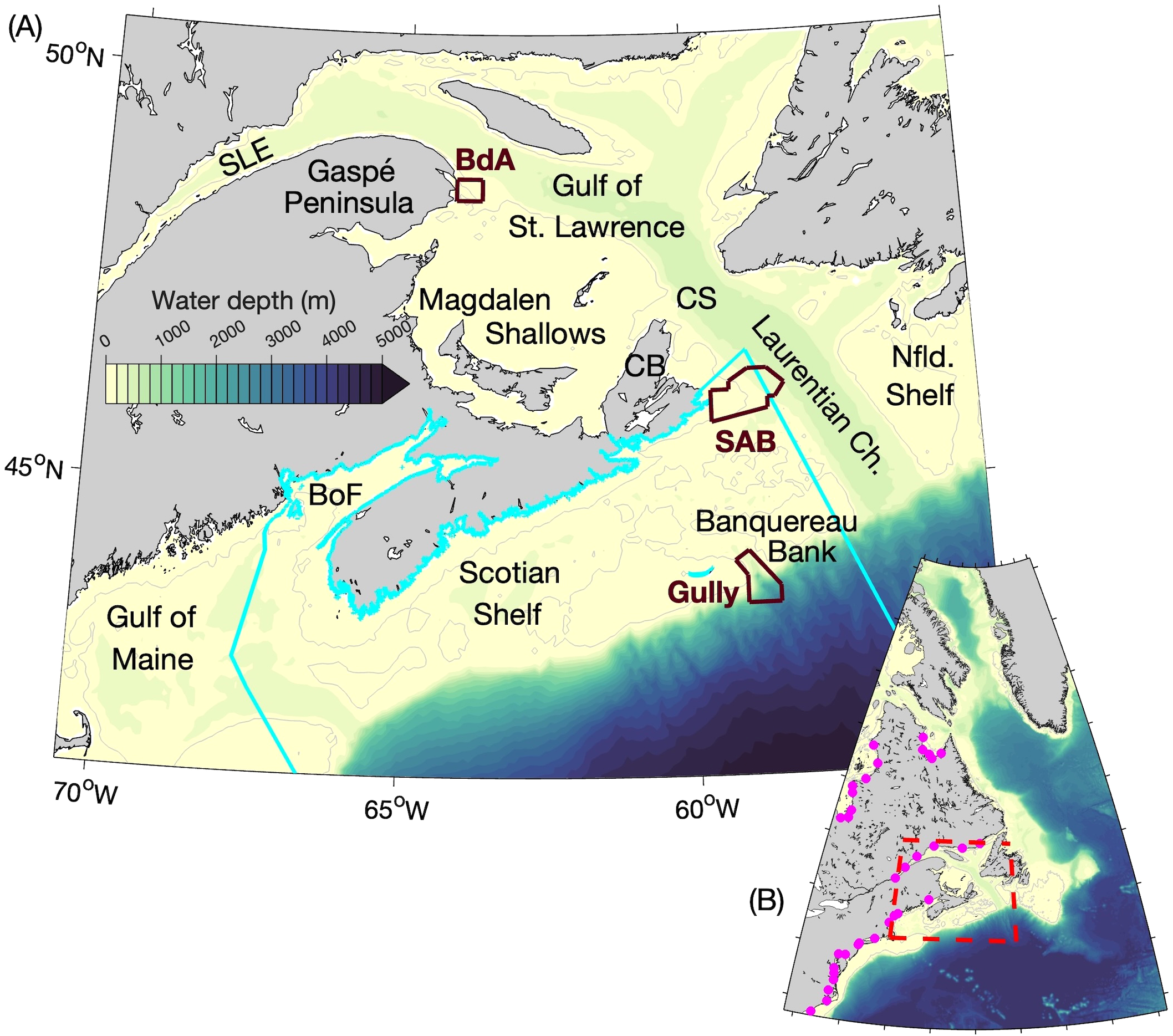
(A) The study area and its bathymetry. The gray lines denote the 100-m depth contours. The cyan line denotes the border of the Scotian Shelf Bioregion. The brown lines denote the borders of Marine Protected Areas (MPAs): Banc-des-Américains (BdA), Saint Anns Bank (SAB), and Gully. The other abbreviations used are: SLE for the St. Lawrence Estuary, CS for Cabot Strait, CB for Cape Breton, Ch. for Channel, Nfld. for Newfoundland, and BoF for the Bay of Fundy. (B) The domain of the circulation model ROMS and sea ice model CICE. The magenta circles denote the locations of river mouths in ROMS. The red dashed line denotes the area shown in (A).
Figure 2
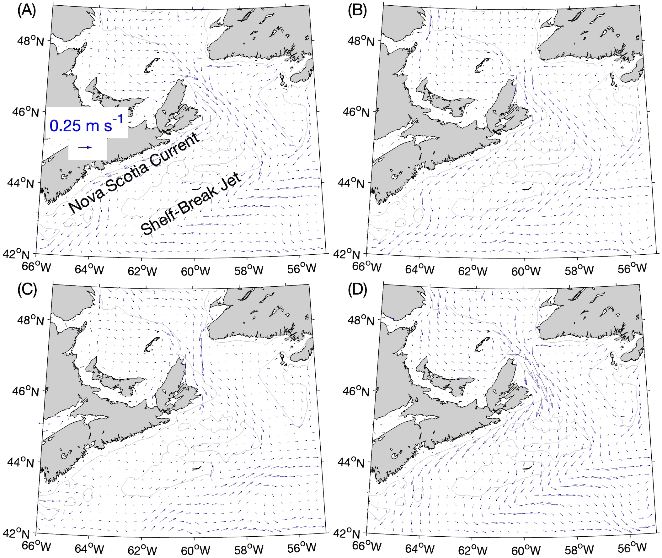
Seasonal-mean simulated currents at the 5-m depth, averaged over the years 2015–2018: (A) winter (1 January–31 March), (B) spring (1 April–30 June), (C) summer (1 July–30 September), and (D) fall (1 October–31 December). The current vectors are shown at every fourth model grid point. The gray lines denote the 100-m depth contours.
The Scotian Shelf Bioregion is high in biodiversity and productivity, because of its geographic, topographic, and aforementioned hydrodynamic complexity. Commercial fishery landings of more than 40 species of finfish and 28 invertebrate species have ranged from 370 to 250 × 106 kg per year since the collapse of the Atlantic cod fishery in the early 1990s (Breeze et al., 2002; MacLean et al., 2013; Rozalska and Coffen-Smout, 2020). American lobster, snow crab, the giant sea scallop, and surfclam constitute the most valuable species landed (Government of Canada, 2017). Virtually all of the ~340 species of fish, macro-invertebrates and seaweeds known from the Scotian Shelf (Ward-Paige and Bundy, 2016) have dispersive larval stages in their life histories. Understanding patterns of biodiversity and productivity for purposes of spatial planning, management, and conservation cannot ignore the role of water movement in determining the distribution of marine organisms through space and time (Siegel et al., 2003; Stortini et al., 2020).
There are currently two MPAs in the Scotian Shelf Bioregion (Figure 1A), the Gully and the Saint Anns Bank (hereafter SAB). The Gully MPA, encompassing a submarine canyon of the same name on the offshore edge of the Scotian Shelf, has a surface area of ~2,300 km2 and is home to a rich ecosystem in which 16 cetacean species and more than 30 coral species have been observed (Fisheries and Oceans Canada, 2017). The SAB MPA, with a surface area of ~5,100 km2, is located just south of the western side of Cabot Strait. The taxonomic affiliations of its biota are more similar to those of the Gulf of St. Lawrence to its north than to the Scotian Shelf on which it is located (Ford and Serdynska, 2013). Given this indicator we also consider another MPA, the Banc-des-Américains (hereafter BdA). It covers 1,000 km2 in the Gulf of St. Lawrence near the tip of the Gaspé Peninsula, where the outflow from the St. Lawrence Estuary turns southeastward towards Cabot Strait. The flow of nutrient-rich waters from the St. Lawrence Estuary and a topography that favours vertical mixing contribute to the biological productivity in this MPA (Fisheries and Oceans Canada, 2019). Its location upstream of the Scotian Shelf makes it a potential source of water that subsequently flows through the SAB and Gully MPAs (Figure 2).
MPAs are a popular component of marine spatial planning that may be designated for diverse purposes. They are, however, fraught with risky issues of policy and implementation decisions (Hatcher and Bradbury, 2006; O’Leary et al., 2012), such that their designation requires thorough analyses and careful pre-planning. (Once made, decisions are rarely reversed.) An emerging strategy is to create networks of MPAs within large ocean domains that are well-enough connected that they have capacity to restore each other in the event of negative disturbances or catastrophes that compromise the effective function of any one MPA within the network (Allison et al., 2003; Commission for Environmental Cooperation, 2012). In this context, which is relevant to Canada’s current strategy (Koropatnik, 2018), MPAs should not only contain unique or representative habitats and biodiversity, they should also serve as sources of reproductive propagules (i.e., spores, eggs, larvae) and emigrants (i.e., mobile juveniles and adults) of species moving beyond the nominal MPA boundaries, and also as sinks for recruits and immigrants of species originating from outside these designated areas. Ideally, to best achieve preservation and conservation goals, the MPAs in a network should contain subpopulations of all the species’ metapopulations that occur in the network domain, making the extinction of any species unlikely because local extirpations can be re-seeded from connected MPAs. This concept of maintaining ecological connectivity through the spatial connections among MPAs is easy to imagine, challenging to model, and very difficult to test empirically. Falsifiable predictions can be made and sometimes tested against measures of genetic distance among sub-populations using molecular genetics techniques (Palumbi, 2003; D’Aloia et al., 2019). Here, we focus on the modelling aspects for a well-known marine domain.
Ecological models are attempts to induce the simplest useful explanation of patterns from observations, or to deduce the simplest possible prediction of patterns from accepted theory. Mature models use both approaches. The modelling of marine ecological connectivity is mature as the result of a remarkable amount of creative research. Meticulous life history observations of fish larvae demonstrate the range of diversity and complexity in pelagic larval development and swimming behaviour (Leis, 2021). Coupled biophysical models have demonstrated the relevance of incorporating these characteristics in numerical simulation models of population connectivity (Werner et al., 2007). The approach taken in this multi-year study is to first develop the best oceanographic models possible for a given domain and management question, and then to examine how relevant the simplest particle tracking solutions can be assuming that dispersal life history stages are conservative with respect to the water mass (Tang et al., 2006; Yang et al., 2008). This approach is mainly of generic value in large domains only; small systems and solutions for particular species require extremely high-resolution grids and time-dependent, species-specific behavioural profiles in response to known environmental cues. Only after calibrating and validating the passive model will we incrementally add life history attributes characteristic of major groups of marine organisms. Regardless of the model assumptions, the best way to predict the connectivity among MPAs is to run many numerical particle-tracking experiments and generate a connectivity probability matrix (e.g., Yang et al., 2008).
Past studies using numerical particle-tracking for conservation efforts in the Scotian Shelf-Gulf of St. Lawrence region focused mainly on circulation patterns within particular MPAs, or on simulating the directed movement of marine animals. Examples of the former include studies by Shan et al. (2014a, 2014b) for the Gully MPA and by Ma et al. (2024) for the Eastern Shore Islands on the Scotian Shelf (where an MPA has been proposed). Marine animals in the region whose movements have been simulated with particle-tracking models include Calanus spp. copepods (e.g.,Zakardjian et al., 2003; Brennan et al., 2024), juvenile Atlantic salmon (Ohashi and Sheng, 2018), and a hypothetical invasive species (Brickman, 2014). Cong et al. (1996) used particle-tracking to calculate retention indices (the inverse of connectivity) on the Scotian Shelf and found a positive correlation between the retention index in spring and the abundance of intermediate-length Atlantic cod in summer over one area of the Shelf. As far as we know, this is the only existing study in which numerical particle-tracking was used to quantify spatial variability in the physical oceanographic state of this region, and to relate this variability to the biological state of the region.
In this study, the seasonal-mean and three-dimensional circulation fields calculated from the 2015–2018 output of a coupled ocean circulation-sea ice model are used by a particle-tracking model to simulate the movement of passive bio-particles (i.e., neutrally buoyant particles that do not undertake any swimming behaviours and whose movements are sums of advection by currents and small, random movements added to represent the effect of sub-grid scale circulation features). Particles are released near the surface in the SAB and BdA MPAs, and particle distributions after 30, 60, and 90 days (representing a realistic range of pelagic larval durations) are composited over 2015–2018 to derive the general patterns of passive particle movement and connectivity among three MPAs. The number of particles located in MPAs downstream from release areas (Gully for the SAB; SAB and Gully for BdA) is examined at the same time intervals as the general patterns of particle distribution. We also briefly discuss year-to-year variability in the experimental results and the effect of varying a parameter in the particle-tracking program that influences the particles' small, random movements. In Section 2, we describe the ocean circulation-sea ice model and the setup of the particle-tracking experiments. Results of the experiments are discussed in Section 3, and a summary of the results as well as directions of future research are presented in Section 4.
2 Methodology
2.1 Numerical ocean circulation-sea ice model
The ocean circulation-sea ice model used in this study is based on the physical component of the three-dimensional (3D) ocean circulation-sea ice-biogeochemistry model known as DalROMS-NWA12 developed by Ohashi et al. (2024). Major changes for this study include the use of: (1) a smoothed bathymetry, (2) the semi-prognostic method (Sheng et al., 2001), and (3) the spectral nudging method (Thompson et al., 2007). These changes are described below along with the model configuration. The reader is referred to Ohashi et al. (2024) for a detailed description of the model.
The ocean circulation module of DalROMS-NWA12 is based on the Regional Ocean Modeling System (ROMS, version 3.9; Haidvogel et al., 2008) and the sea ice module is based on the Community Ice CodE (CICE, version 5.1; Hunke et al., 2015). The two modules are coupled in a manner similar to that of Kristensen et al. (2017) using the Model Coupling Toolkit (version 2.10; Jacob et al., 2005; Larson et al., 2005). The circulation and sea ice modules use the same horizontal grid and bathymetry. The model grid covers the area between ~81° W and ~39° W and between ~33.5° N and ~76° N (Figure 1B). Each model grid cell spans ~1/12° in the east-west direction and are nearly square-shaped, measuring ~8 km on each side near the grid’s southern boundary and ~2 km on each side near the northern boundary. In the vertical direction, ROMS uses 40 layers configured in the terrain-following S-coordinate system, originally developed by Song and Haidvogel (1994). In the S-coordinate system, spacing between the S-layers is finer near the surface and bottom than at mid-depths in deep waters, and more uniform in shallow waters. The model bathymetry is derived from the 1/240°-resolution data set GEBCO_2019 (GEBCO Compilation Group, 2019). In any numerical model that uses terrain-following vertical layers, a balance needs to be struck between smoothing the bathymetry in areas with sharp gradients (e.g., shelf breaks and seamounts) to reduce computational errors and avoiding excessive smoothing that makes the model bathymetry unrealistic (e.g.,Sikirić et al., 2009). In the case of Ohashi et al. (2024), after the GEBCO_2019 bathymetry was linearly interpolated to the model grid, the only smoothing applied was over seamounts in deep waters using the filter developed by Shapiro (1975). In this study, smoothing was applied to the entire model bathymetry.
At the sea surface, the circulation and sea ice modules of DalROMS-NWA12 are forced by atmospheric fields derived from the hourly reanalysis known as the European Center for Mid-Range Weather Forecasting Reanalysis v5 (ERA5; Hersbach et al., 2020) which has a horizontal grid spacing of 1/4°. Daily inputs of temperature, salinity, and currents for ROMS, as well as sea ice concentration and sea ice thickness for CICE, at the lateral open boundaries of DalROMS-NWA12 are derived from the daily reanalysis dataset known as the Global Ocean Physics Reanalysis (GLORYS; Lellouche et al., 2021) which has a horizontal grid spacing of 1/12°. Tidal elevation and currents derived from the global tidal model solution TPXO9v2a (based on the model of Egbert and Erofeeva (2002)), which has a horizontal grid size of 1/6° and 15 tidal constituents, are also specified at the lateral open boundaries of the ocean module. Freshwater input from 35 rivers is specified at the heads of channels cut into the model coastline to represent the rivers. For the St. Lawrence River, this freshwater input is derived from a dataset of monthly-mean flow at the city of Québec (Fisheries and Oceans Canada, 2023a) which is estimated from observed water levels using the regression model of Bourgault and Koutitonsky (1999). For all other rivers, the freshwater input is derived from the monthly-mean dataset of Dai (2021), with averages for the years 1900–2018 used for months with no data. Freshwater input along the coast due to melting snow and ice cover over land is derived from the monthly-mean dataset of Bamber et al. (2018).
Yang et al. (2023) demonstrated that a barotropic version of the ocean circulation module performs well in simulating tides and storm surges. Ohashi et al. (2024) compared the results of two 3D ocean-sea ice simulations to satellite and in situ observations. In one simulation, the modelled temperature and salinity were nudged towards a blend of in situ observations and reanalysis, while in the other simulation no nudging was applied. While both simulations reproduced the major features of the circulation and of the temperature, salinity, and sea ice distributions, the results of the nudged simulation were generally more realistic than the results of the un-nudged simulation. A major feature that was reproduced more accurately in the nudged simulation was the separation of the Gulf Stream and the West Greenland Current from their respective coasts. Chassignet and Xu (2017) showed that decreasing the horizontal grid size of their circulation model from 1/12° to 1/50° resulted in a more realistic simulation of the Gulf Stream, while Pennelly and Myers (2020) reached a similar conclusion about simulating the West Greenland Current. Given that the horizontal resolution of our model grid is ~1/12°, it is possible that this resolution is one reason our model, in the absence of nudging, has difficulty in simulating the two currents.
In this study, we use two methods, not used in Ohashi et al. (2024), to reduce the model’s systematic bias and drift: the semi-prognostic method (Sheng et al., 2001) and the spectral nudging method (Thompson et al., 2007). In the semi-prognostic method, the hydrostatic equation is modified from its original form, , to:
where p is pressure, z is the vertical coordinate, is the density calculated from the simulated temperature and salinity, is the density calculated from long-term averages of the observed temperature and salinity, and α is a coefficient between 0 and 1 (set to 0.5 in this study). Modifying the hydrostatic equation into the form shown in Equation 1 results in there being, effectively, an extra term in the horizontal momentum equations. This extra term can be seen as representing processes that are not resolved in the model. The modification of the horizontal momentum equations in turn affects the advection terms in the tracer equations that govern the simulated temperature and salinity. The simulated temperature and salinity are not themselves nudged towards observed values, making them free of phase errors that would result in the case of direct nudging (Pierce, 1996). In this study, the semi-prognostic method is applied at all model grid cells.
In the spectral nudging method (Thompson et al., 2007), the model temperature and salinity variables are nudged towards the long-term mean of its observed counterpart on relatively long time scales (the mean as well as the annual and semi-annual cycles in this study). Outside of these time scales, the model state is allowed to evolve freely. Thus, this method helps keep the model state realistic on the seasonal or longer time scales while retaining the effect of, for example, storms passing through the model domain. In this study, the spectral nudging method is applied to the simulated temperature and salinity at depths greater than 40 m, in order to prevent this method from interfering with surface fluxes of heat and fresh water. The circulation fields produced by the ocean circulation-sea ice model with the semi-prognostic and spectral nudging methods are realistic, and detailed comparisons between simulated fields and observations will be made in a future study (B. Yang et al., in prep.).
In this study, we use the 3D current fields for the years 2015–2018 produced by DalROMS-NWA12 in a simulation initialised on 1 September 2013 with an ice-free ocean. The initial state of the ocean was derived by interpolating GLORYS ocean reanalysis data for this date to the model grid. Daily-mean current fields were saved and further averaged into seasonal means as described below.
2.2 Numerical particle-tracking experiments
The numerical particle-tracking model used in this study is ROMSPath (Hunter et al., 2022), which is designed for use with ROMS output in offline particle-tracking experiments (i.e., the experiments are run separately from the ocean circulation model whose simulated currents are used as inputs for the experiments). Given a simulated circulation field and the initial positions of particles, ROMSPath uses the fourth-order Runge-Kutta method to calculate the movement of each particle over time due to the simulated currents.
To simulate the effect of processes on scales smaller than that of the circulation model grid, small horizontal and vertical movements in random directions can be added. Taking movement along the x-axis as an example, this additional random movement is calculated as (Visser, 1997):
where R is a normally-distributed random number with zero mean, r is the standard deviation of R, KM is a constant horizontal diffusivity with a user-defined value, and is the time step of the particle-tracking program. In this study, r in Equation 2 is set to 1, the default value of KM is 10 m2 s-1, is 10 minutes, and the option of adding vertical random movements is not used.
Seasonal-mean current fields calculated from daily means for the years 2015–2018 are used as inputs for the particle-tracking experiments, since the main focus of this study is the time-averaged, large-scale patterns of connectivity among the protected areas within and upstream of the Scotian Shelf Bioregion and the year-to-year variability in those patterns. Winter is defined as January–March, spring as April–June, summer as July–September, and fall as October–December. It should be noted that, although the simulated sea ice fields are not used in the particle-tracking experiments, they have an indirect influence on the experiments because they interact with the simulated circulation fields used in the experiments (primarily by modifying the surface stress felt by the ocean). The Gulf of St. Lawrence is the southernmost location bordering the North Atlantic Ocean where sea ice appears regularly (e.g.,Galbraith et al., 2024).
In all numerical experiments, particles are released from either the Saint Anns Bank (SAB) or the Banc-des-Américains (BdA) MPA (Figure 1A). Within every ROMS grid cell whose centre is located within one of these MPAs, 400 particles are released at the 5-m depth in a 20 × 20 grid, resulting in 42,400 particles being released from SAB and 10,000 particles from BdA. All particles are released at the beginning of the experiment. The range of water depths in the MPAs, based on the model bathymetry, is 38 m to 390 m (with an average of 161 m) for SAB and 57 m to 150 m (with an average of 98 m) for BdA. The results of these experiments are discussed in terms of distributions of particles at 30, 60, and 90 days from their release in the case of SAB; for BdA, the particle distribution 30 days after release is not presented since all particles are still located in the Gulf of St. Lawrence. The distributions are composited across the years 2015–2018 for each season and are discussed in terms of the percentage of the total number of particles released over 2015–2018 (169,600 for SAB and 40,000 for BdA) that are located within a ROMS grid cell (an area of ~6 km × ~6 km) or within an MPA (i.e., located in a ROMS grid cell whose centre lies within an MPA). The year-to-year variability in the particle distributions is discussed in a qualitative manner. For BdA, two additional experiments were conducted in which the horizontal diffusivity KM is changed from the default value of 10 m2 s-1 to 5 m2 s-1 and 20 m2 s-1 to examine the effect of this parameter on experimental results.
3 Results
3.1 Saint Anns Bank
The four-year (2015–2018) composites of the distribution of particles released from the Saint Anns Bank (SAB) MPA after 30, 60, and 90 days are presented respectively in Figures 3–5, along with the 2015–2018 means of seasonal-mean currents simulated by ROMS at the 5-m depth (which were also shown in Figure 2). In all three snapshots, a strong contrast is evident between the summer (Figures 3C, 4C, 5C) and the other seasons, with the particles in summer spreading and moving downstream more slowly. This is consistent with the four-year mean of seasonal currents being weakest in the summer.
Figure 3
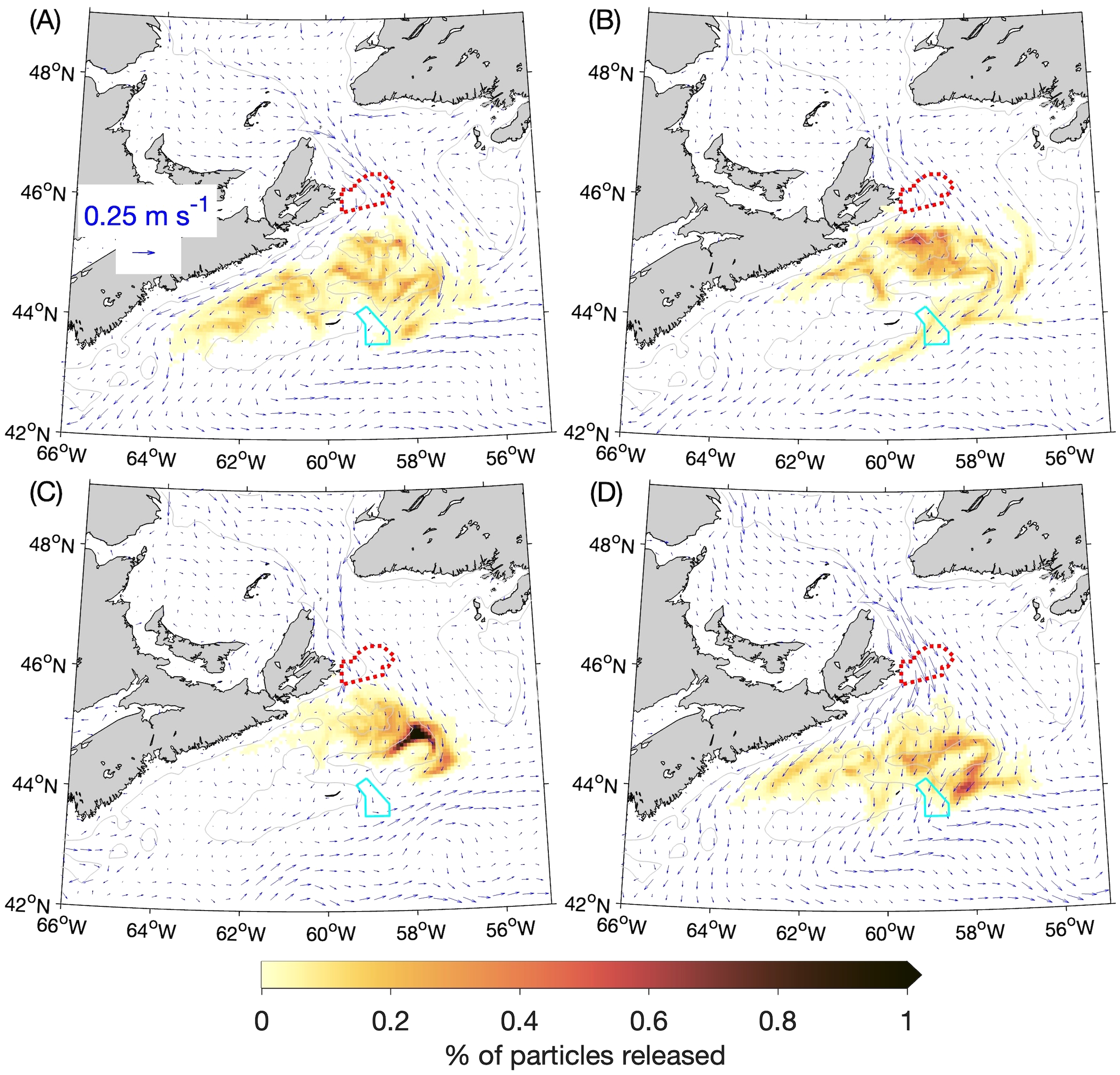
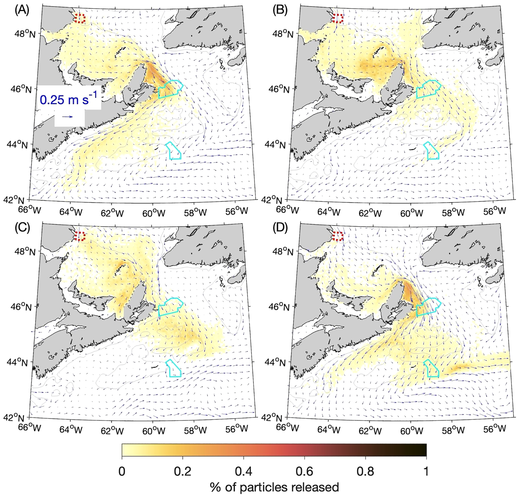
Percentages of particles released at the 5-m depth from the Saint Anns Bank MPA (outlined with the red dotted line) that are located within a given ROMS grid box (about 6 km × 6 km) after 30 days: (A) winter, (B) spring, (C) summer, and (D) fall. The distributions of particles after 30 days from four experiments (for the years 2015–2018) are composited for each season, and the percentages are calculated with respect to the total number of particles released over the four annual experiments (169,600). The cyan solid line denotes the outline of the Gully MPA. The gray lines denote the 100-m depth contours.
Figure 4
Similar to Figure 3 but showing the particle distributions in: (A) winter, (B) spring, (C) summer, and (D) fall 60 days after release.
Figure 5
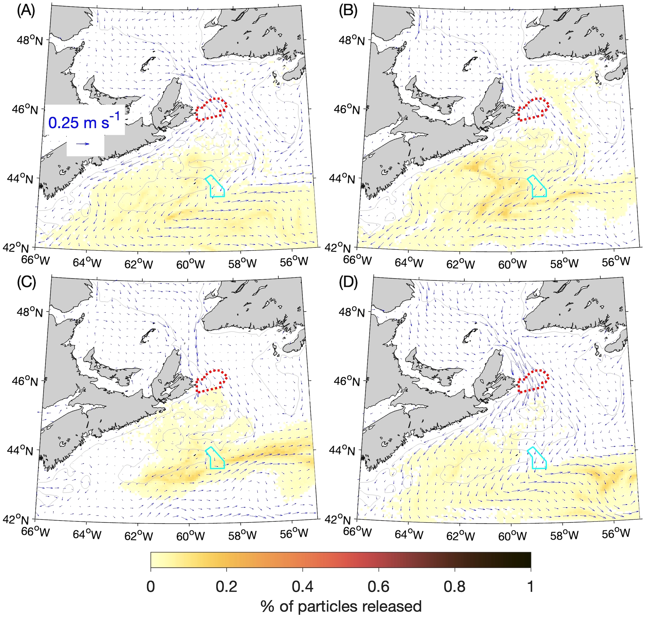
Similar to Figure 3 but showing the particle distributions in: (A) winter, (B) spring, (C) summer, and (D) fall 90 days after release.
After 30 days, the particles released in the winter, spring and fall (Figures 3A, B, D) are in a patch with two branches, one along the coast of Nova Scotia and the other along the shelf break (reflecting the bifurcation of the flow through Cabot Strait), with the rate of particle spread varying between the branches and among the seasons. Particles released in the summer (Figure 3C) are concentrated most densely over the eastern, offshore corner of the Scotian Shelf (up to ~1.4% of all particles released over 2015–2018 per ~6 km × ~6 km area). This area, known as Banquereau Bank, is the site of an Arctic surfclam fishery (Fisheries and Oceans Canada, 2023b) and, although a detailed investigation is beyond the scope of this study, this result raises the possibility that SAB might act as a source of, for example, nutrients or food for the ecosystem over this bank.
The particle distributions at 60 and 90 days after release (Figures 4A-D, 5A-D) show that, in all four seasons, the particles move equatorward over time along the Scotian Shelf while also spreading across the Shelf. In the summer at 60 days after release (Figure 4C) there is a relatively high concentration of particles in the vicinity of the Gully MPA. About 11% of particles released from SAB are located within the Gully MPA itself at this time (Table 1). After 90 days the patch of particles is quite diffuse in all four seasons, but almost 2% of the particles released in the summer are still located within the Gully MPA. These results suggest that, for passive particles, the SAB and Gully MPAs are most strongly connected during the summer at time scales of about 60 days. Figure 6 illustrates the year-to-year variability in the experimental results by showing the outlines of particle patches at day 60 from each year, which were shown in composite form in Figure 4. The outlines are represented by the contours of 0.005% of the particles released during 2015–2018. They show that, although variations among years do exist in the particle movements, the findings discussed above are generally true for all four years (e.g., the particles released in the summer moving more slowly than in the other seasons and being concentrated near the Gully MPA after 60 days). The results of the BdA experiments display more distinct differences among the years (see following section).
Table 1
| Winter (JFM) | Spring (AMJ) | Summer (JAS) | Fall (OND) | |
|---|---|---|---|---|
| Days since release | ||||
| 30 days | 0.13 | 1.11 | 0 | 1.25 |
| 60 days | 1.45 | 2.08 | 10.51 | 1.60 |
| 90 days | 0.13 | 0.75 | 1.90 | 0.0029 |
Percentage of particles released from Saint Anns Bank MPA each season over four years (169,600 particles) that are within the Gully MPA 30, 60, and 90 days after release.
The horizontal diffusivity in the particle-tracking program is 10 m2 s-1 in all experiments.
Figure 6
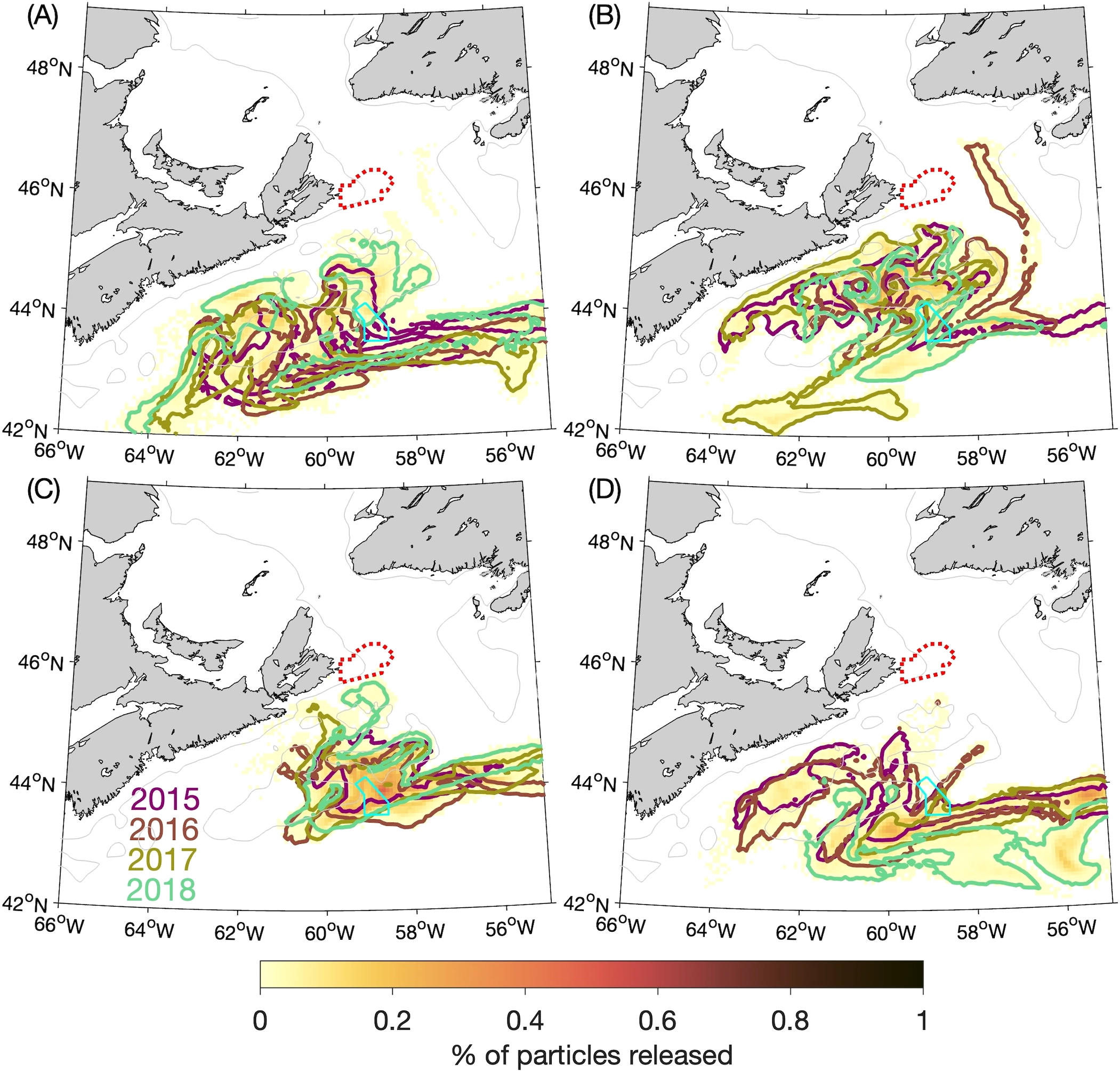
Similar to Figure 4 (percentages of particles released at the 5-m depth from the Saint Anns Bank MPA that are located within a given ROMS grid box after 60 days) but additionally showing the outlines of particle patches in: (A) winter, (B) spring, (C) summer, and (D) fall from individual years. The outlines are represented by the 0.005% contour. (The percentages are calculated with respect to the total number of particles released over the four annual experiments, i.e., in the same manner as for the four-year composite distributions shown with the colour shading.).
Although the focus of this study is on the particles’ horizontal movement, they can also undergo significant vertical movements during the experiments. The maximum depths reached by the particles range from about 13 m (spring) to 33 m (fall) after 30 days, 20 m (spring) to 56 m (fall) after 60 days, and 79 m (summer) to 380 m (spring) after 90 days. These vertical movements are due solely to advection by simulated currents and do not reflect vertical migrations of plankton (i.e., directed vertical movement due to buoyancy adjustments or locomotion).
3.2 Banc-des-Américains
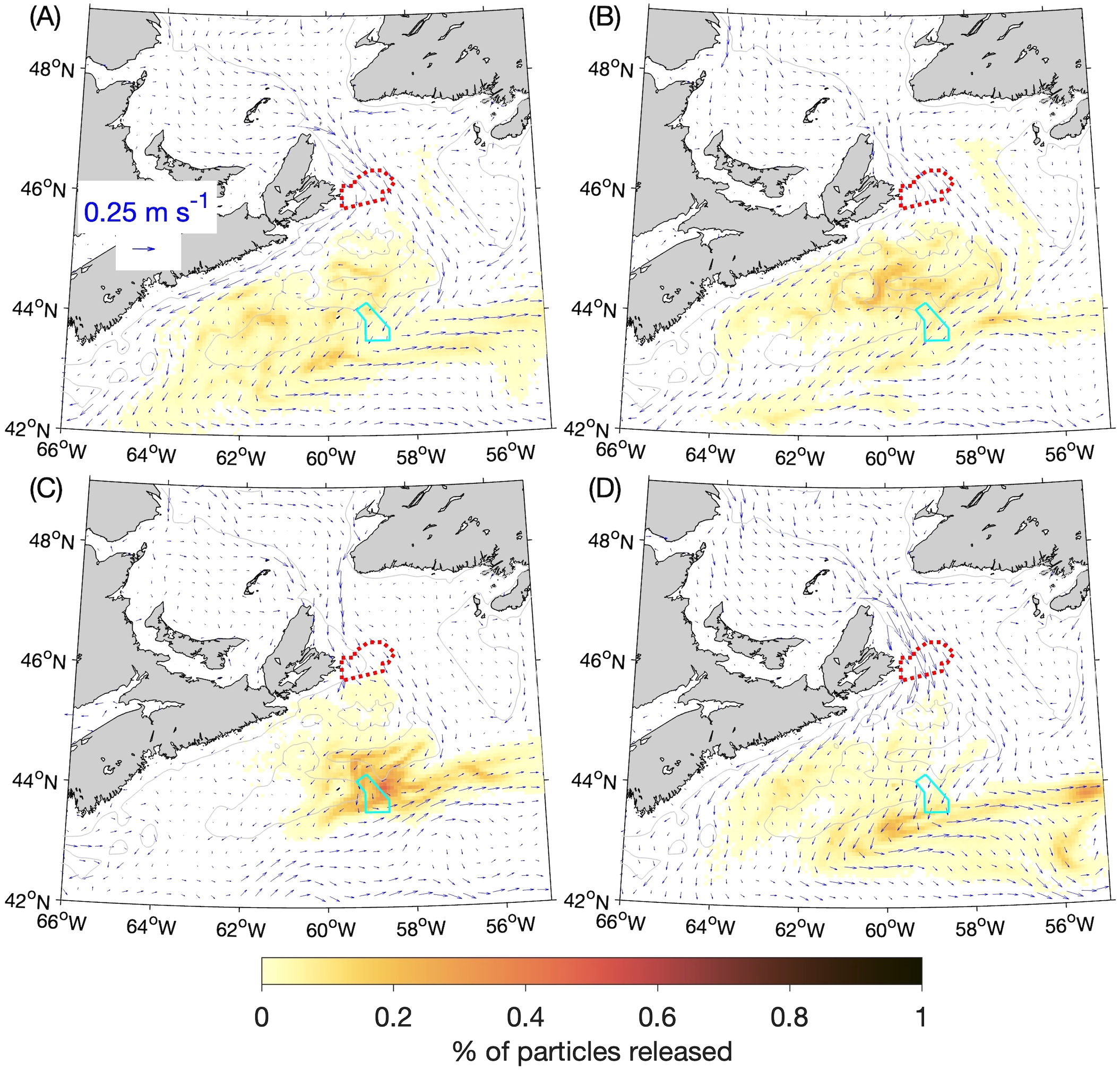
The four-year composites of particle distributions for each season, 60 and 90 days after release from the Banc-des-Américains (BdA) MPA, are presented respectively in Figures 7 and 8. The day 60 distributions can be divided into winter and fall on one hand (Figures 7A, D) and spring and summer (Figures 7B, C) on the other. In the winter and fall, when currents along the coast of the Magdalen Shallows in the southwest Gulf of St. Lawrence are stronger, particles tend to accumulate along the coast just inside of and along Cabot Strait. In the spring and summer, more particles bypass the Magdalen Shallows and spread across Cabot Strait as they exit the Gulf of St. Lawrence. In the day 90 distributions (Figures 8A-D), the patch of particles that had accumulated near and within Cabot Strait during winter and fall are hugging the coast as they move through the Strait (Figures 8A, D). The contrast between winter–fall and spring–summer in the particles’ movement is also evident after the particles move through Cabot Strait onto the Scotian Shelf. In winter and fall they move predominantly along the coast of Nova Scotia, while in the spring and summer there are more particles that cross the Scotian Shelf and turn equatorward at the shelf break.
Figure 7
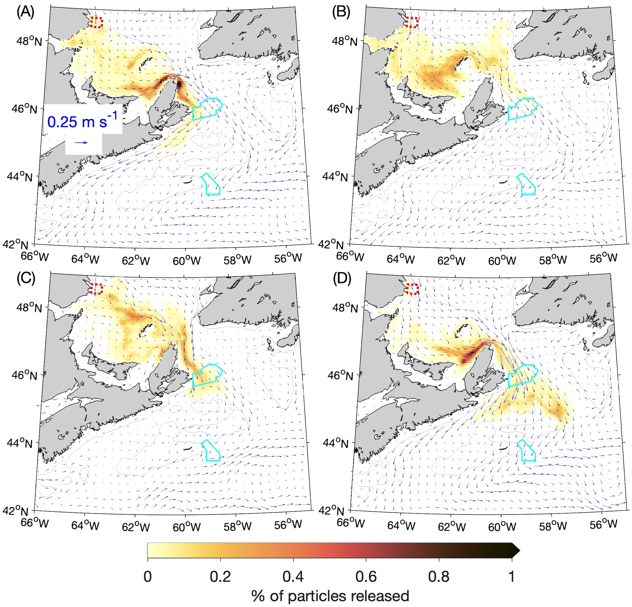
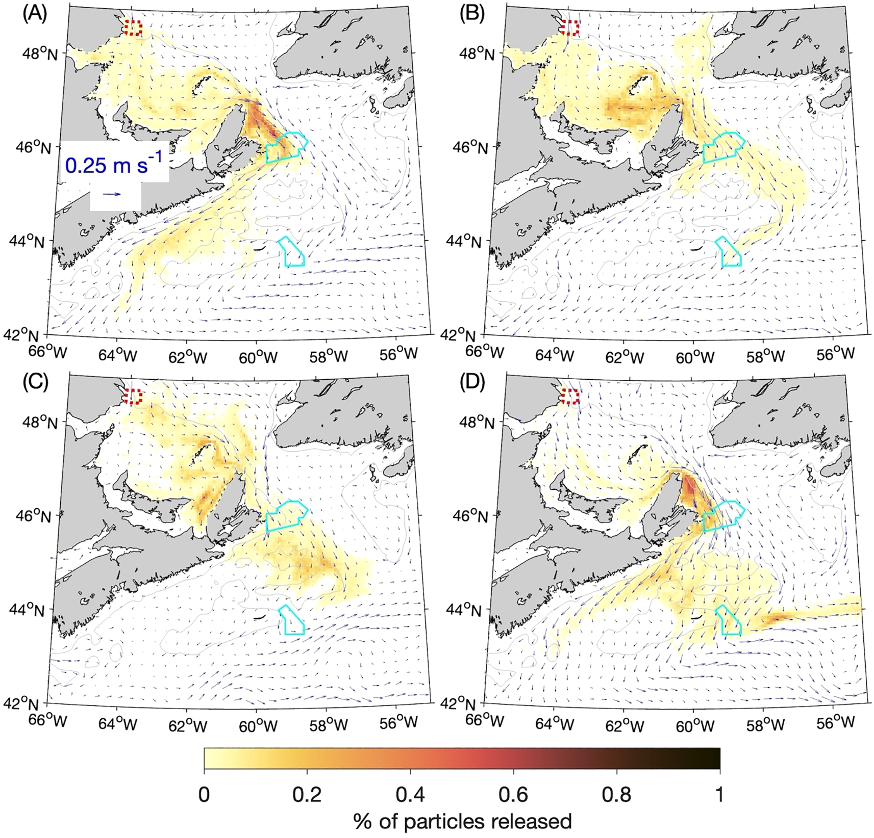
Percentages of particles released at the 5-m depth from the Banc-des-Américains MPA (outlined with a red dotted line) that are located within a given ROMS grid box (about 6 km × 6 km) after 60 days: (A) winter, (B) spring, (C) summer, and (D) fall. The distributions of particles after 60 days from four experiments (for the years 2015–2018) are composited for each season, and the percentages are calculated with respect to the total number of particles released over the four annual experiments (40,000). The cyan solid lines denote the outlines of the Saint Anns Bank and Gully MPAs. The gray lines denote the 100-m depth contours.
Figure 8
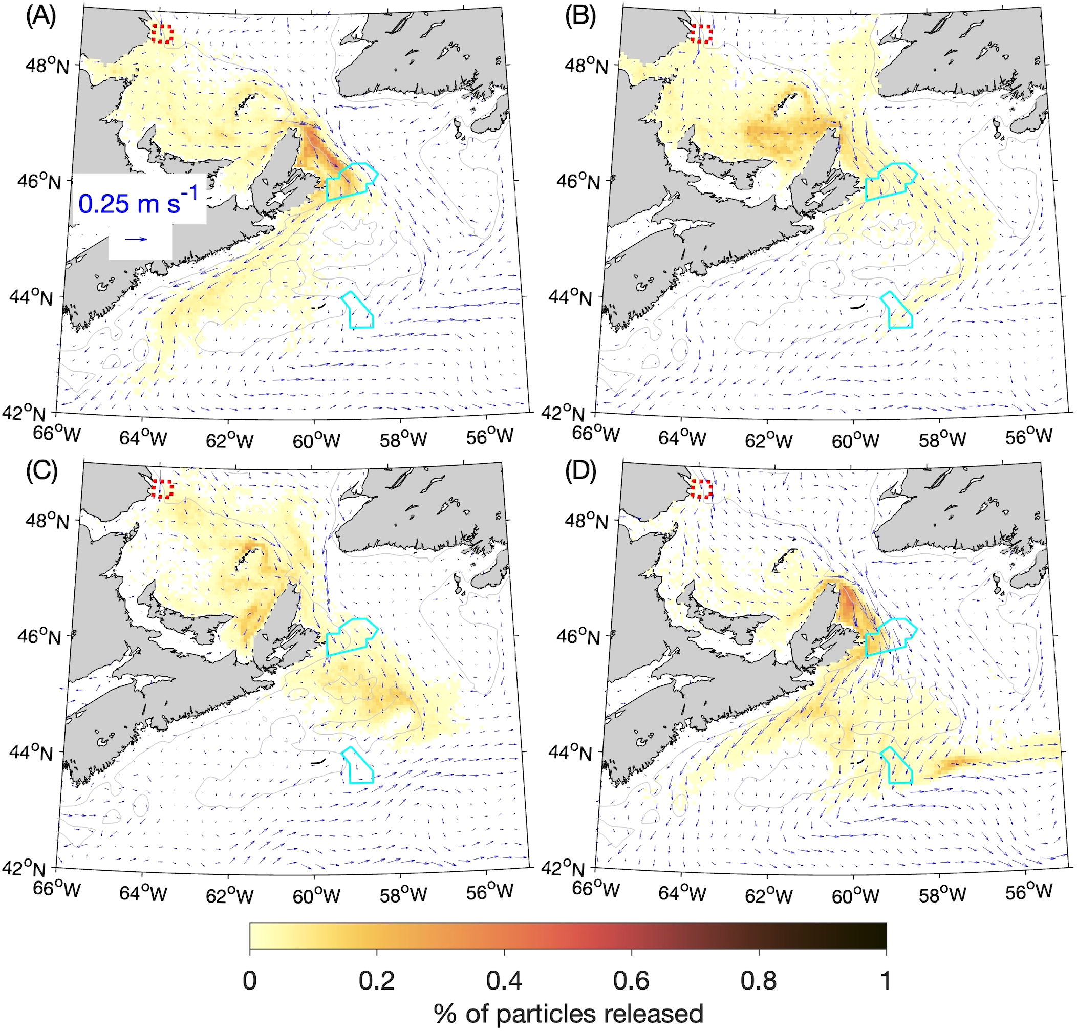
Similar to Figure 7 but showing the particle distributions in: (A) winter, (B) spring, (C) summer, and (D) fall 90 days after release.
The SAB MPA, located just west of the Laurentian Channel (Figure 1), is well situated to have particles from BdA pass through it, regardless of whether they are moving in the fall-winter or spring-summer pattern. About 5% of the particles released in the summer are in the SAB MPA after 60 days (Table 2), and the percentage of particles there after 90 days ranges from 1% in summer to 8% in winter. Particles only reach the Gully MPA after 90 days in the spring and fall (about 0.1% and 2% respectively; Table 2), although this result for the spring is due to just one of the four annual experiments.
Table 2
| Particles in Saint Anns Bank MPA | |||||||
|---|---|---|---|---|---|---|---|
| Winter | Spring | Summer | Fall | ||||
| Days since release | |||||||
| Horizontal diffusivity = 10 m2 s-1 | |||||||
| 60 days | 1.45 | 0.17 | 5.15 | 2.31 | |||
| 90 days | 8.16 | 3.13 | 1.06 | 4.94 | |||
| Horizontal diffusivity = 5 m2 s-1 | |||||||
| 60 days | 1.32 (-8.82%) | 0.12 (-29.23%) | 4.93 (-4.23%) | 2.09 (-9.62%) | |||
| 90 days | 8.29 (+1.51%) | 3.17 (+1.44%) | 0.98 (-7.31%) | 5.01 (+1.42%) | |||
| Horizontal diffusivity = 20 m2 s-1 | |||||||
| 60 days | 1.88 (+29.93%) | 0.26 (+60.00%) | 5.01 (-2.62%) | 2.34 (+1.19%) | |||
| 90 days | 8.04 (-1.56%) | 2.99 (-4.32%) | 1.29 (+21.93%) | 4.45 (-9.92%) | |||
| Particles in Gully MPA | |||||||
| Winter | Spring | Summer | Fall | ||||
| Days since release | |||||||
| Horizontal diffusivity = 10 m2 s-1 | |||||||
| 90 days | 0 | 0.14 | 0 | 1.73 | |||
| Horizontal diffusivity = 5 m2 s-1 | |||||||
| 90 days | 0 | 0.09 (-31.48%) | 0 | 1.88 (+8.70%) | |||
| Horizontal diffusivity = 20 m2 s-1 | |||||||
| 90 days | 0.0025 | 0.12 (-14.81%) | 0.0025 | 1.77 (+2.46%) | |||
Percentage of particles released from the Banc-des-Américains MPA each season over four years (40,000 particles) that are within the Saint Anns Bank MPA after 60 and 90 days and in the Gully MPA after 90 days, using horizontal diffusivities of 10, 5, and 20 m2 s-1 in the particle-tracking program.
(None of the particles are in SAB 30 days after release, or in the Gully MPA 30 or 60 days after release.) In the case of experiments with horizontal diffusivities of 5 m2 s-1 and 20 m2 s-1, the changes relative to experiments with a horizontal diffusivity of 10 m2 s-1 are shown in parentheses. The underlined lines of text are subheadings denoting experimental settings.
Year-to-year variability in the results of the BdA experiments is illustrated in Figures 9A-D, which shows the outlines of the particle patches after 90 days for each year. (The outlines are defined in the same manner as in Figure 6.) Year-to-year variability in the particle distributions over the Scotian Shelf is small in the summer (Figure 9C) but more evident in the other seasons, such as between 2018 and the other years in terms of propagation along the coast of Nova Scotia in winter (Figure 9A). In the spring (Figure 9B), the shelf-break branch of the particle patch is only present in 2017, which means that the ~0.1% of the particles located in the Gully MPA at day 90 in the spring experiments is entirely due to the 2017 experiment. Details of the causes of year-to-year variabilities in the input variables and output of the ocean circulation-sea ice model are beyond the scope of this study, but a possible factor is the discharge of the St. Lawrence River. Monthly-mean discharge values (estimated from water level observations and used as one of the inputs of the circulation-ice model) are shown in Figure 10. The discharge during spring and summer is higher in 2017 than in the other years, with the peak discharge in 2017 (~24,600 m3 s-1) being about 55% higher than the average peak discharge of the other three years (~15,900 m3 s-1). The mechanism behind the bifurcation of the outflow from Cabot Strait has not yet been fully studied, but our results suggest the St. Lawrence River’s discharge plays an important role.
Figure 9
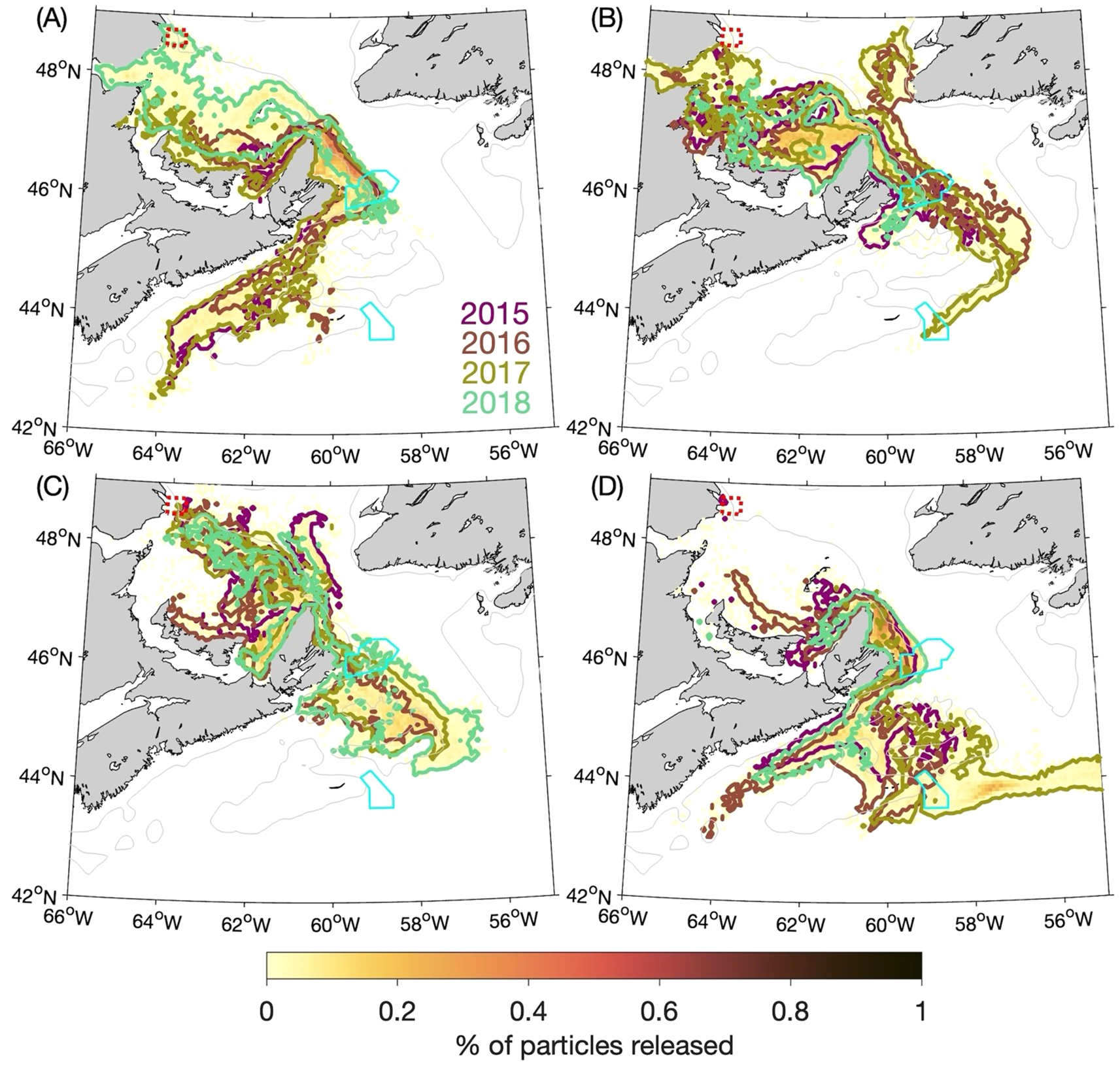
Similar to Figure 8 (percentages of particles released at the 5-m depth from the Banc-des-Américains MPA that are located within a given ROMS grid box after 90 days) but additionally showing the outlines of particle patches in: (A) winter, (B) spring, (C) summer, and (D) fall from individual years. The outlines are represented by the 0.005% contour. (The percentages are calculated with respect to the total number of particles released over the four annual experiments, i.e., in the same manner as for the four-year composite distributions shown with the colour shading.).
Figure 10
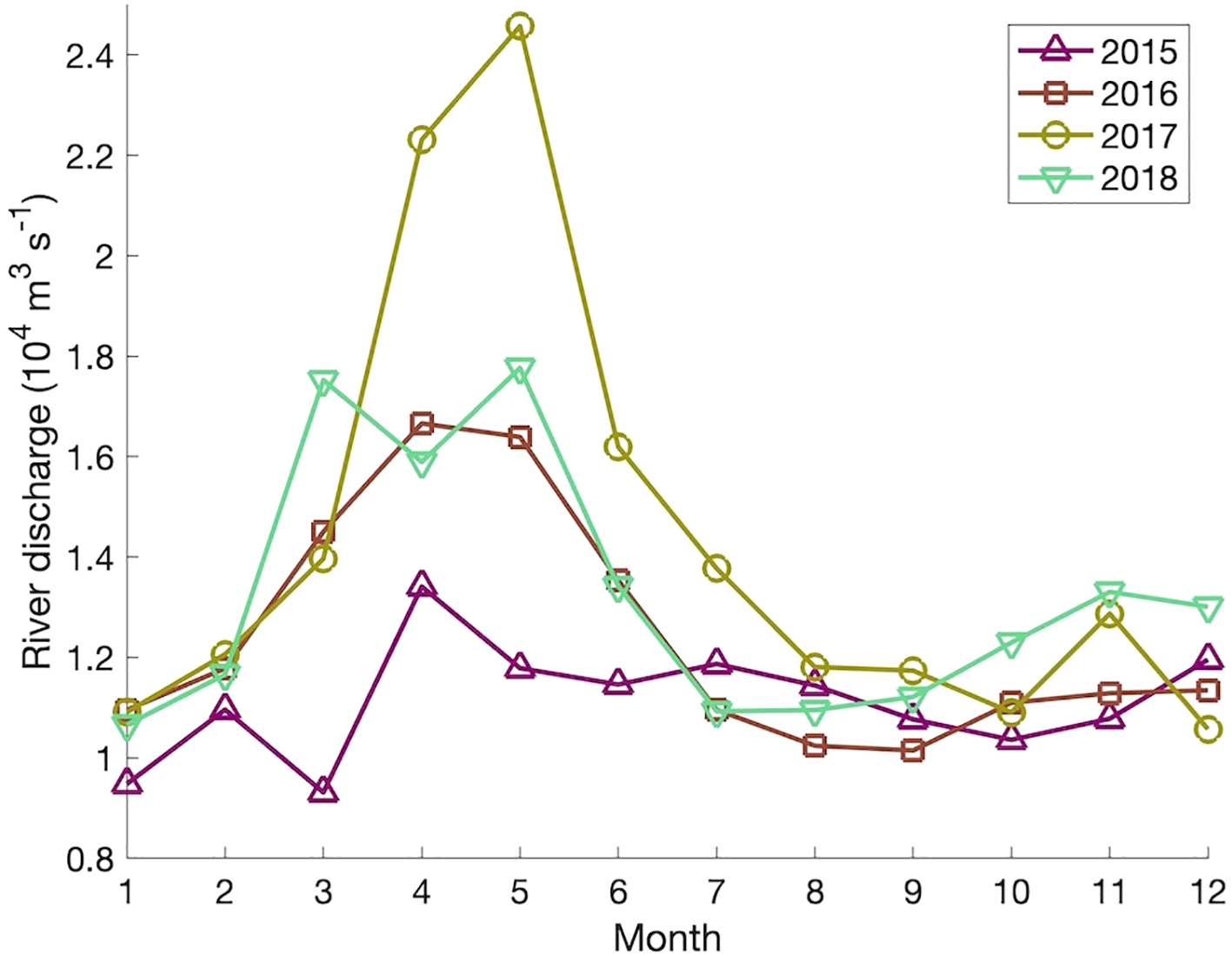
Monthly-mean discharge of the St. Lawrence River at Québec for the years 2015–2018, estimated from observed water levels using the regression model of Bourgault and Koutitonsky (1999) (Fisheries and Oceans Canada, 2023a).
3.3 Effect of horizontal diffusivity in the particle-tracking model
In the experiments discussed so far, the horizontal diffusivity KM in the numerical particle-tracking program (which controls the small, random movements that represent the effects of sub-grid scale circulation features) was set to 10 m2 s-1. Because the value of this parameter is set by the user and there is an ad hoc aspect to it, we repeated the BdA experiments with KM set to 5 m2 s-1 and 20 m2 s-1. The distributions of particles from these experiments after 90 days are shown in Figures 11 and 12 respectively. They are generally similar to their counterparts from the experiments using the default KM value of 10 m2 s-1 (Figure 8). As expected, when particles become concentrated (e.g., along the western side of Cabot Strait in winter and fall), the patches are denser when KM is smaller (Figure 11 vs. Figure 8) and sparser when KM is larger (Figure 12 vs. Figure 8). Because the major findings discussed in Section 3.2 focused on occurrences of high particle concentrations, they are fairly robust to changes in the horizontal diffusivity. As shown in Table 2, the percentage of particles reaching SAB after 90 days in winter (~8%) changes by ~+2% and ~-2% respectively, and the percentage reaching SAB after 60 days in summer (~5%) changes by ~-4% and ~-3% respectively when KM is halved or doubled from the default value. Much larger relative variations occur for lower concentrations of particles, such as the percentage in SAB after 60 days in spring (0.17%) that changes by ~-29% and +60% respectively when KM is halved or doubled. This is expected, given that KM represents the effect of small-scale turbulent eddy diffusion superimposed on the larger, directed movements of particles due to advection by the simulated currents. These results indicate that it is important to test different values of this user-defined parameter to ensure that the conclusions derived from the experiments are not highly sensitive to its value.
Figure 11
Similar to Figure 8 (percentages of particles released at the 5-m depth from the Banc-des-Américains MPA that are located within a given ROMS grid box in: (A) winter, (B) spring, (C) summer, and (D) fall after 90 days) but for experiments in which the horizontal diffusivity in the numerical particle-tracking model was decreased from 10 m2 s-1 to 5 m2 s-1.
Figure 12
Similar to Figure 11 but for experiments in which the horizontal diffusivity in the numerical particle-tracking model was increased to 20 m2 s-1: (A) winter, (B) spring, (C) summer, and (D) fall.
3.4 Comparison between experimental results and the distribution of snow crab
The numerical particle-tracking model used in this study bases its simulation of particle movements on the output of an ocean circulation-sea ice model whose performance has been validated against observations (Ohashi et al., 2024); but the output of the particle-tracking model itself is not validated in the current study. Validation of the results of numerical particle-tracking experiments could be achieved through, for example, comparison with measurements of environmental DNA (e.g.,Andruszkiewicz et al., 2019) or surveys of larvae using light traps (e.g.,Rasmuson et al., 2022). Here, we compare our results with available information on the distribution of the snow crab, a commercially important and thus regularly monitored marine species in Atlantic Canadian waters.
The snow crab (Chionocetes opilio) is found in all three MPAs examined in this study (Fisheries and Oceans Canada (2016) for the Gully, Jeffery et al. (2025) for SAB, and Fisheries and Oceans Canada (2025a) for BdA). Its eggs are hatched between late spring and early summer, and the planktonic larval stage lasts three to four months (Fisheries and Oceans Canada, 2025b). Thus, the duration of our experiments (three months) matches the low end of the snow crab’s pelagic larval duration, during which the larvae are neutrally buoyant and poor swimmers. On the Scotian Shelf, the largest concentration of mature snow crab tends to occur in Cabot Strait and the eastern part of the shelf, with relatively high concentrations also occurring along the coast of Nova Scotia and along the shelf break (e.g., Figure 45 of Choi and Zisserson (2008)).
In our experiments in which particles are released into the seasonal-mean currents for spring and summer, after 90 days, between ~1 and ~2% of particles from SAB are within the Gully MPA (Table 1) and between 1 and 3% of the particles from BdA are in SAB (Table 2). In addition, the distribution of particles from BdA after 90 days in the summer (Figure 8C) is consistent with that of mature snow crab in that the concentration of particles on the Scotian Shelf is highest (~0.2% of all particles released) on the eastern part of the shelf, with the cloud of particles also extending along the coast of Nova Scotia and along the shelf break. Our results suggest that, although (to the best of our knowledge) the three MPAs in our study were designated without connectivity among them in mind, the BdA and SAB MPAs act as source areas to downstream MPAs of an important marine species. These results, together with the distribution of particles from SAB after 30 days discussed in Section 3.1, suggest the eastern end of the Scotian Shelf (and its offshore corner in particular) as an area to consider for future protection as a source.
4 Discussion and conclusions
In this study, the three-dimensional (3D) currents produced by the coupled, numerical ocean circulation-sea ice model known as DalROMS-NWA12 (Ohashi et al., 2024) were used as input for the numerical particle-tracking model ROMSPath in experiments designed to examine the general patterns of ecological connectivity among Marine Protected Areas (MPAs) off the Atlantic coast of Canada. Seasonally-averaged, 3D currents for the years 2015–2018 were used to simulate the movements of passive particles released near the sea surface in three MPAs: Banc-des-Américains (BdA) in the Gulf of St. Lawrence, Saint Anns Bank (SAB) in Cabot Strait, and the Gully on the offshore edge of the Scotian Shelf. The passive particles can be seen as representing many types of marine organisms in their dispersive, early life history stages, but without any ability move themselves in a directed fashion. As such, the results represent the null biological condition whereby physics alone determines the number of offspring arriving at one area from others in a spatial network. We acknowledge that the null assumption is not true for most marine species (e.g.,Leis, 2021), but argue that the null model is necessary to evaluate the significance of biological mechanisms affecting larval dispersal. We suggest that in energetic, shelf-scale systems over the time scales of metapopulation dynamics the null model may prove suitable decision support for the design of networks of marine protected areas.
Results of the particle-tracking experiments yielded particle distributions over biologically relevant pelagic larval durations (30, 60, and 90 days after release), and composited intra- and inter-annual variability over a 4 year period (2015–2018) that reflects several life cycles of most organisms in the region. The strongest connection among the three MPAs considered is predicted to be between the SAB and Gully MPAs in the summer (~11% of particles released from SAB were in the Gully MPA after 60 days), followed by BdA and SAB in the winter (~8% of released particles were in SAB after 90 days). About 0.1% of the particles released from BdA in the spring were in the Gully MPA after 90 days in 2017, a year when discharge from the St. Lawrence River was unusually large. When the BdA experiments were repeated with the horizontal diffusivity in ROMSPath (which controls the small, random movements that represent the effect of sub-grid scale circulation features) halved or doubled, the number of particles in SAB after 90 days in winter increased or decreased by ~2% respectively. The magnitudes of these physical connectivity values indicate how important physical oceanographic processes are in the dispersal of bioparticles in this region, and raises the question of how much they could be increased by directed locomotion of larvae.
The predicted movements of passive particles examined in this study shed light on the circulation-mediated connections among biologically productive areas in our study region. To be more useful to conservation efforts, further studies should examine the movement and fate of bioparticles that are more representative of marine organisms in this region. There are four major ways in which this study can be expanded to extend predictions of what is physically possible for all passive particles to what is ecologically probable for particular types of bioparticles within the model domains (Werner et al., 2007; Wolanski and Kingsford, 2014; Leis, 2021).
The first way is to add biological processes to living bioparticles (such as reproductive propagules of nektonic or benthic species and other types of meroplankton such as algal spores). These processes include directed swimming behaviours (such as prey searching, predator avoidance, horizontal and vertical migrations in response to environmental cues), and time-dependent transitions of life stages due to the settlement or recruitment of larvae and reproductive propagules, or their mortality due to starvation or predation. The latter two types of processes represent losses of bioparticles from the model within its spatial domain, which are additional to losses of bioparticles from the domain due to advection beyond the geographical boundary of the domain. Adding mortality to the passive-particle experiments will diminish the percentage of released particles that reach the MPAs represented in this study, while the addition of swimming behaviours can increase or decrease particle dispersion, depending on the effectiveness of behaviours that favour retention (particularly in gyres, eddies and the benthic boundary layer). Realistic subroutines to be coded in future particle-tracking model runs include horizontal swimming in random directions or towards cues (such as phytoplankton or salinity), diel vertical migrations, and transitions from passive drifting to directed swimming towards certain seabed types at a predetermined age.
Results are expected to differ significantly between experiments with and without swimming, as well as between experiments that include different swimming behaviours. Ohashi and Sheng (2016) demonstrated, for the St. Lawrence Estuary, that simulated movements of particles can differ dramatically between, for example, particles that swim horizontally in random directions and those that swim towards higher salinity. The results of experiments using passive, immortal particles that are presented in this study are not representative of the actual or observed movements of all dispersive propagules of marine species in our study area (and it would be computationally prohibitive to model each of the species even if the necessary parameter values were known). But comparisons of results for four or five functional classes of dispersal life histories is expected to provide insights to the degree to which various biological process alter the patterns of connectivity among MPAs in contrast to the predictions of a physical model. Note also the importance of directed swimming in response to environmental cues. If the larval swimming, no matter how strong, is undirected or directed only for short periods in variable directions (such as prey searching; Wolanski and Kingsford, 2014), then it is apparently random motion at model cell scales, and may be simulated simply by increasing the value of the horizontal diffusivity term in the particle tracking model.
The second way in which this study can be extended is the use of additional particle release areas and release depths. Along the Atlantic coast of Canada there are five additional MPAs, in areas ranging from southern Labrador to the Bay of Fundy (Government of Canada, 2024), and four “Areas of Interest” being considered for MPA designation (two in the Gulf of St. Lawrence and two on the Scotian Shelf; Government of Canada, 2022). Inclusion of these additional areas is expected to enhance the insights gained in this study on the connectivity within the Scotian Shelf-Gulf of St. Lawrence region and, in the case of the Areas of Interest, to allow an estimation of the impact they will have as MPAs. Experiments in which particles are released at different depths, with or without active swimming behaviour, are expected to reflect variations with depth of the circulation field as well as the effect of the thermocline during the warmer seasons.
Thirdly, the spatial and temporal resolutions of the circulation fields used in the particle-tracking experiments can be increased. The spatial resolution can be increased by, for example, nesting a domain with a smaller horizontal grid size in the existing 1/12° domain. As discussed in Section 2.1, decreasing the horizontal grid size from 1/12° to 1/50° or less has been shown to improve the performance of models in simulating key circulation features in the northwest Atlantic (Chassignet and Xu, 2017; Pennelly and Myers, 2020). On the temporal side, a major limitation of this study is the use of seasonally-averaged currents as inputs for our particle-tracking experiments. The effect of high-frequency variability (such as those caused by tides or storms) can be included by using circulation model results that are saved at a higher frequency (e.g., hourly or daily). Then, the average pattern of connectivity for a given season and year can be found by conducting a 90-day experiment centred on each day of that season and averaging the results of those 90 experiments. This process can then be repeated for each year to find the interannual variability in the connectivity. Although this approach was not used in this study due to its large computational cost, experiments conducted in this manner should yield results that are different from those of experiments in which seasonally-averaged circulation fields are used, as we did in this study. Comparing the two sets of results should provide insights into the areas and seasons in which temporal variability of O(1 day) in the circulation exerts a strong influence.
Finally, the particle-tracking experiments can be conducted using circulation fields simulated under future climate scenarios. Brennan et al. (2016) examined the potential effects, on marine animals in our study region, of lower dissolved oxygen and higher temperatures in the future (which are expected if observed trends continue). Simulated circulation fields also undergo changes when near-surface waters are warmer (Peng et al., 2022), which in turn is likely to alter connectivity patterns. Particle-tracking experiments in which the ambient ocean temperature or salinity is used as a cue for swimming would be affected by changes in both the circulation field and the behaviour cue. Taking into account possible changes under future climate conditions should make our conclusions more robust for application to marine conservation efforts.
Statements
Data availability statement
The datasets presented in this study can be found in online repositories. The names of the repository/repositories and accession number(s) can be found below: https://zenodo.org/records/14548211 (ROMSPath with time-invariant circulation field option. Zenodo).
Author contributions
KO: Conceptualization, Formal Analysis, Investigation, Methodology, Software, Visualization, Writing – original draft, Writing – review & editing. JS: Conceptualization, Funding acquisition, Resources, Supervision, Writing – review & editing. BH: Conceptualization, Funding acquisition, Resources, Supervision, Writing – review & editing.
Funding
The author(s) declare financial support was received for the research and/or publication of this article. This study is part of the project “Modelling Ecological Connectivity among Canada’s Atlantic Marine Protected Areas during the Anthropocene” funded by Fisheries and Oceans Canada. JS also acknowledges support from the National Science and Engineering Research Council of Canada’s Discovery Grant program.
Acknowledgments
We thank Bo Yang (Ocean University of China) for sharing with us the results of his ocean circulation-sea ice simulation, conducted during his sabbatical at Dalhousie University. We thank Sarah Smith (Cape Breton University) for sharing her research on the marine species present in our study area. The ocean circulation-sea ice simulation and the numerical particle-tracking experiments were carried out on computing resources maintained by the Digital Research Alliance of Canada. We are grateful for the constructive comments provided by the reviewers and the editor, which led to the addition of Section 3.4 as well as many other enhancements to this article. Maps in this study were generated using the package M_Map (Pawlowicz, 2020). The colour maps used in this study are by Thyng et al. (2016) and Crameri (2018).
Conflict of interest
The autors declare that the research was conducted in the absence of any commercial or financial relationships that could be construed as a potential conflict of interest.
Generative AI statement
The author(s) declare that no Generative AI was used in the creation of this manuscript.
Any alternative text (alt text) provided alongside figures in this article has been generated by Frontiers with the support of artificial intelligence and reasonable efforts have been made to ensure accuracy, including review by the authors wherever possible. If you identify any issues, please contact us.
Publisher’s note
All claims expressed in this article are solely those of the authors and do not necessarily represent those of their affiliated organizations, or those of the publisher, the editors and the reviewers. Any product that may be evaluated in this article, or claim that may be made by its manufacturer, is not guaranteed or endorsed by the publisher.
References
1
Allison G. W. Gaines S. D. Lubchenco J. Possingham H. P. (2003). Ensuring persistence of marine reserves: Catastrophes require adopting an insurance factor. Ecol. Appl.13, S8–24. doi: 10.1890/1051-0761(2003)013[0008:EPOMRC]2.0.CO;2
2
Andruszkiewicz E. A. Roseff J. R. Fringer O. B. Ouellette N. T. Lowe A. B. Edwards C. A. et al . (2019). Modeling environmental DNA transport in the coastal ocean using Lagrangian particle tracking. Front. Mar. Sci.6. doi: 10.3389/fmars.2019.00477
3
Angulo-Valdés J. A. Hatcher B. G. (2010). A new typology of benefits derived from marine protected areas. Mar. Policy34, 635–644. doi: 10.1016/j.marpol.2009.12.002
4
Bamber J. L. Tedstone A. J. King M. D. Howat I. M. Enderlin E. M. van den Broeke M. R. et al . (2018). Land ice freshwater budget of the arctic and North Atlantic oceans: 1. Data, methods, and results. J. Geophys. Res. Oceans123, 1827–1837. doi: 10.1002/2017JC013605
5
Bourgault D. Koutitonsky V. G. (1999). Real-time monitoring of the freshwater discharge at the head of the St. Lawrence Estuary. Atmos.-Ocean37, 203–220. doi: 10.1080/07055900.1999.9649626
6
Breeze H. Fenton D. G. Rutherford R. J. Silva M. A. (2002). The Scotian Shelf: An Ecological Overview for Ocean Planning. (Can. Tech. Rep. Fish. Aquat. Sci. 2393) (Dartmouth, NS, Canada: Bedford Institute of Oceanography). Available online at: https://publications.gc.ca/site/eng/422206/publication.html (Accessed August 17, 2025).
7
Brennan C. E. Blanchard H. Fennel K. (2016). Putting temperature and oxygen thresholds of marine animals in context of environmental change: A regional perspective for the Scotian Shelf and Gulf of St. Lawrence. PloS One11, e0167411. doi: 10.1371/journal.pone.0167411
8
Brennan C. E. Maps F. Lavoie D. Plourde S. Johnson C. L. (2024). Modelling the complete life cycle of an arctic copepod reveals complex trade-offs between concurrent life cycle strategies. Prog. Oceanogr.229, 103333. doi: 10.1016/j.pocean.2024.103333
9
Brickman D. (2014). Could ocean currents be responsible for the west to east spread of aquatic invasive species in Maritime Canadian waters? Mar. pollut. Bull.85, 235–243. doi: 10.1016/j.marpolbul.2014.05.034
10
Chassignet E. P. Xu X. (2017). Impact of horizontal resolution (1/12° to 1/50°) on gulf stream separation, penetration, and variability. J. Phys. Oceanogr.47, 1999–2021. doi: 10.1175/JPO-D-17-0031.1
11
Choi J. S. Zisserson B. M. (2008). An assessment of the snow crab resident on the Scotian Shelf in 2006, focusing upon CFA 4X (Can. Sci. Advis. Sec. Res. Doc. 2008/003) (Darmouth, NS, Canada: Bedford Institute of Oceanography).
12
Commission for Environmental Cooperation (2012). Guide for Planners and Managers to Design Resilient Marine Protected Area Networks in a Changing Climate (Montreal, Canada: Commission for Environmental Cooperation). Available online at: http://www.cec.org/files/documents/publications/10856-guide-planners-and-managers-design-resilient-marine-protected-area-networks-in-en.pdf (Accessed August 17, 2025).
13
Cong L. Sheng J. Thompson K. R. (1996). A retrospective study of particle retention on the outer banks of the Scotian Shelf 1956-1993 (Can. Tech. Rep. Hydrogr. Ocean Sci. 170) (Dartmouth, NS, Canada: Bedford Institute of Oceanography). Available online at: https://publications.gc.ca/site/eng/9.805846/publication.html (Accessed August 17, 2025).
14
Crameri F. (2018). Scientific colour maps (Zenodo). doi: 10.5281/zenodo.1243862
15
D’Aloia C. C. Naujokaitis-Lewis I. Blackford C. B. Chu C. Curtis J. M. R. Darling E. S. et al . (2019). Coupled networks of permanent protected areas and dynamic conservation areas for biodiversity conservation under climate change. Front. Ecol. Evol.7. doi: 10.3389/fevo.2019.00027
16
Dai A. (2021). Hydroclimatic trends during 1950–2018 over global land. Clim. Dynam.56, 4027–4049. doi: 10.1007/s00382-021-05684-1
17
Dinerstein E. Vynne C. Sala E. Joshi A. R. Fernando S. Lovejoy T. E. et al . (2019). A Global Deal For Nature: Guiding principles, milestones, and targets. Sci. Adv.5, eaaw2869. doi: 10.1126/sciadv.aaw2869
18
Du J. Zhang W. G. Li Y. (2022). Impact of Gulf Stream Warm-Core Rings on slope water intrusion into the Gulf of Maine. J. Phys. Oceanogr.52, 1797–1815. doi: 10.1175/JPO-D-21-0288.1
19
Egbert G. D. Erofeeva S. Y. (2002). Efficient inverse modeling of Barotropic ocean tides. J. Atmos. Ocean. Tech.19, 183–204. doi: 10.1175/1520-0426(2002)019<0183:EIMOBO>2.0.CO;2
20
Fisheries and Oceans Canada (2016). Eastern Nova Scotia and 4X Snow crab (Chionoecetes opillio) – Effective as of 2013. Available online at: https://waves-vagues.dfo-mpo.gc.ca/library-bibliotheque/4083556x.pdf (Accessed August 17, 2025).
21
Fisheries and Oceans Canada (2017). The Gully Marine Protected Area Management Plan, Second Edition. Available online at: https://waves-vagues.dfo-mpo.gc.ca/library-bibliotheque/4083556x.pdf.
22
Fisheries and Oceans Canada (2019). Review of ecosystem features, indicators and surveys for ecological monitoring of the Banc-des-Américains Marine Protected Area (Can. Sci. Advis. Sec. Sci. Advis. Rep. 2019/033) (Mont-Joli, QC, Canada: Maurice Lamontagne Institute). Available online at: https://publications.gc.ca/site/eng/9.880772/publication.html (Accessed August 17, 2025).
23
Fisheries and Oceans Canada (2023a). Monthly Freshwater Runoffs of the St. Lawrence at the Height of Quebec City. Available online at: https://catalogue.ogsl.ca/en/dataset/ca-cioos_84a17ffc-4898-4261-94de-4a5ea2a9258d (Accessed August 17, 2025).
24
Fisheries and Oceans Canada (2023b). Stock status update of Arctic surfclam (Mactromeris polynyma) on Banquereau and Grand Bank to the end of the 2022 fishing season (Can. Sci. Advis. Sec. Sci. Resp. 2023/039) (Dartmouth, NS, Canada: Bedford Institute of Oceanography). Available online at: https://publications.gc.ca/collections/collection_2024/mpo-dfo/fs70-7/Fs70-7-2023-039-eng.pdf (Accessed August 17, 2025).
25
Fisheries and Oceans Canada (2025a). Banc-des-Américains Marine Protected Area (MPA) annual report 2023. Available online at: https://www.dfo-mpo.gc.ca/oceans/publications/mpaannualreports-rapportsannuelszpm/2023/american-americains-eng.html (Accessed August 17, 2025).
26
Fisheries and Oceans Canada (2025b). Snow crab. Available online at: https://www.dfo-mpo.gc.ca/species-especes/profiles-profils/snow-crab-crabe-neiges-atl-eng.html (Accessed August 17, 2025).
27
Ford J. Serdynska A. (Eds.) (2013). Ecological Overview of St Anns Bank (Can. Tech. Rep. Fish. Aquat. Sci. 3023) (Dartmouth, NS, Canada: Bedford Institute of Oceanography). Available online at: https://publications.gc.ca/site/eng/447606/publication.html (Accessed August 17, 2025).
28
Fratantoni P. S. Pickart R. S. (2007). The western north Atlantic shelfbreak current system in summer. J. Phys. Oceanogr.37, 2509–2533. doi: 10.1175/JPO3123.1
29
Galbraith P. S. Sévigny C. Bourgault D. Dumont D. (2024). Sea ice interannual variability and sensitivity to fall oceanic conditions and winter air temperature in the Gulf of St. Lawrence, Canada. J. Geophys. Res. Oceans129, e2023JC020784. doi: 10.1029/2023JC020784
30
Gatien G. (1976). A study in the Slope Water region south of Halifax. J. Fish. Res. Board Can.33, 2213–2217. doi: 10.1139/f76-270
31
GEBCO Compilation Group (2019). GEBCO_2019 Grid. doi: 10.5285/836f016a-33be-6ddc-e053-6c86abc0788e
32
Government of Canada (2017).2016 Value of provincial landings. Available online at: https://www.dfo-mpo.gc.ca/stats/commercial/land-debarq/sea-maritimes/s2016pv-eng.htm (Accessed February 25, 2025).
33
Government of Canada (2018).Map of bioregions. Available online at: https://www.dfo-mpo.gc.ca/oceans/maps-cartes/bioregions-eng.html (Accessed December 30, 2024).
34
Government of Canada (2022).Oceans act areas of interest. Available online at: https://open.Canada.ca/data/en/dataset/32bf34ea-d51f-46c9-9945-563989dfcc7b (Accessed December 30, 2024).
35
Government of Canada (2023 ). Protecting Canada’s oceans by 2030 and beyond . Available online at: https://www.dfo-mpo.gc.ca/oceans/conservation/plan/MCT-OCM-eng.html (Accessed December 30, 2024).
36
Government of Canada (2024).Marine Protected Areas across Canada. Available online at: https://www.dfo-mpo.gc.ca/oceans/mpa-zpm/index-eng.html (Accessed December 30, 2024).
37
Haidvogel D. B. Arango H. Budgell W. P. Cornuelle B. D. Curchitser E. Di Lorenzo E. et al . (2008). Ocean forecasting in terrain-following coordinates: Formulation and skill assessment of the Regional Ocean Modeling System. J. Comput. Phys.227, 3595–3624. doi: 10.1016/j.jcp.2007.06.016
38
Hannah C. G. Shore J. A. Loder J. W. Naimie C. E. (2001). Seasonal circulation on the western and central Scotian shelf. J. Phys. Oceanogr.31, 591–615. doi: 10.1175/1520-0485(2001)031<0591:SCOTWA>2.0.CO;2
39
Hatcher B. G. Bradbury R. (2006). “Ocean ecosystem management: How much greater is the whole than the sum of the parts?,” in Towards Principled Oceans Governance: Australian and Canadian Approaches and Challenges. Eds. RothwellD. R.VanderZwaagD. L. (Routledge, Oxford), 205–235.
40
Hersbach H. Bell B. Berrisford P. Hirahara S. Horányi A. Muñoz-Sabater J. et al . (2020). The ERA5 global reanalysis. Q. J. R. Meteor. Soc146, 1999–2049. doi: 10.1002/qj.3803
41
Hunke E. C. Lipscomb W. H. Turner A. K. Jeffery N. Elliott S. (2015). CICE: The Los Alamos sea ice model documentation and software user’s manual version 5.1 LA-CC-06-012 (Los Alamos, NM, U.S.A: Los Alamos National Laboratory).
42
Hunter E. J. Fuchs H. L. Wilkin J. L. Gerbi G. P. Chant R. J. Garwood J. C. (2022). ROMSPath v1.0: Offline particle tracking for the Regional Ocean Modeling System (ROMS). Geosci. Model. Dev.15, 4297–4311. doi: 10.5194/gmd-15-4297-2022
43
Jacob R. Larson J. Ong E. (2005). M × N communication and parallel interpolation in community climate system model version 3 using the model coupling toolkit. Int. J. High Perform. Comput. Appl.19, 293–307. doi: 10.1177/1094342005056116
44
Jeffery N. W. Daigle R. Cameron B. J. Glass A. Harbin J. Pettitt-Wade H. et al . (2025). Analysis of the enhanced snow crab survey for monitoring conservation priorities in St. Anns Bank Marine Protected Area (Can. Tech. Rep. Fish. Aquat. Sci. 3650) (Dartmouth, NS, Canada: Bedford Institute of Oceanography). Available online at: https://publications.gc.ca/site/eng/9.945328/publication.html (Accessed August 17, 2025).
45
Koropatnik T. (Ed.) (2018). Proceedings of the regional science peer review of design guidance for a network of Marine Protected Areas in the Scotian Shelf Bioregion (Part 1): July 6–7, 2016. (Can. Sci. Advis. Sec. Proceed. Ser. 2018/002) (Dartmouth, NS, Canada: Bedford Institute of Oceanography). Available online at: https://publications.gc.ca/site/eng/9.854779/publication.html (Accessed August 17, 2025).
46
Kristensen N. M. Debernard J. B. Maartensson S. Wang K. Hedstrom K. (2017). metno/metroms: Version 0.3 - before merge (Version v0.3) (Zenodo). doi: 10.5281/zenodo.1046114
47
Larson J. Jacob R. Ong E. (2005). The model coupling toolkit: A new fortran90 toolkit for building multiphysics parallel coupled models. Int. J. High Perform. Comput. Appl.19, 277–292. doi: 10.1177/1094342005056115
48
Leis J. M. (2021). Perspectives on larval behaviour in biophysical modelling of larval dispersal in marine, demersal fishes. Oceans2, 1–25. doi: 10.3390/oceans2010001
49
Lellouche J.-M. Greiner E. Bourdallé-Badie R. Garric G. Angélique M. Drévillon M. et al . (2021). The copernicus global 1/12° Oceanic and sea ice GLORYS12 reanalysis. Front. Earth Sci.9. doi: 10.3389/feart.2021.698876
50
Ma Y. Wu Y. Jeffery N. W. Horwitz R. Xu J. Horne E. et al . (2024). Simulating dispersal in a complex coastal environment: The Eastern Shore Islands archipelago. ICES J. Mar. Sci.81, 178–194. doi: 10.1093/icesjms/fsad193
51
MacLean M. Breeze H. Walmsley J. Corkum J. (Eds.) (2013). State of the Scotian Shelf Report. (Can. Tech. Rep. Fish. Aquat. Sci. 3074) (Dartmouth, NS, Canada: Bedford Institute of Oceanography). Available online at: https://publications.gc.ca/site/eng/465879/publication.html (Accessed August 17, 2025).
52
Mulongoy K. J. Gidda S. B. (2008). The value of nature: Ecological, economic, cultural and social benefits of protected areas (Montreal, Canada: Secretariat of the Convention on Biological Diversity). Available online at: https://www.mybis.gov.my/pb/2342 (Accessed August 17, 2025).
53
O’Leary B. C. Brown R. L. Johnson D. E. von Nordheim H. Ardron J. Packeiser T. et al . (2012). The first network of marine protected areas (MPAs) in the high seas: The process, the challenges and where next. Mar. Policy36, 598–605. doi: 10.1016/j.marpol.2011.11.003
54
Ohashi K. Laurent A. Renkl C. Sheng J. Fennel K. Oliver E. (2024). DalROMS-NWA12 v1.0, a coupled circulation–ice–biogeochemistry modelling system for the northwest Atlantic Ocean: development and validation. Geosci. Model. Dev.17, 8697–8733. doi: 10.5194/gmd-17-8697-2024
55
Ohashi K. Sheng J. (2016). Influence of St. Lawrence River discharge on the circulation and hydrography in Canadian Atlantic waters. Cont. Shelf Res.58, 32–49. doi: 10.1016/j.csr.2013.03.005
56
Ohashi K. Sheng J. (2018). Study of Atlantic salmon post-smolt movement in the Gulf of St. Lawrence using an individual-based model. Reg. Stud. Mar. Sci.24, 113–132. doi: 10.1016/j.rsma.2018.08.012
57
Palumbi S. R. (2003). Population genetics, demographic connectivity, and the design of marine reserves. Ecol. Appl.13, S146–S158. doi: 10.1890/1051-0761(2003)013[0146:PGDCAT]2.0.CO;2
58
Pawlowicz R. (2020). M_Map: A mapping package for MATLAB, version 1.4m (Vancouver, BC, Canada: Department of Earth, Ocean, and Atmospheric Sciences, The University of British Columbia). Available online at: https://www.eoas.ubc.ca/~rich/map.html. (Accessed August 17, 2025)
59
Peng Q. Xie S.-P. Wang D. Huang R. X. Chen G. Shu Y. et al . (2022). Surface warming-induced global acceleration of upper ocean currents. Sci. Adv.8, eabj8394. doi: 10.1126/sciadv.abj8394
60
Pennelly C. Myers P. G. (2020). Introducing LAB60: A 1/60° NEMO 3.6 numerical simulation of the Labrador Sea. Geosci. Model. Dev.13, 4959–4975. doi: 10.5194/gmd-13-4959-2020
61
Pierce D. W. (1996). Reducing phase and amplitude errors in restoring boundary conditions. J. Phys. Oceanogr.26, 1552–1556. doi: 10.1175/1520-0485(1996)026%3C1552:RPAAEI%3E2.0.CO;2
62
Rasmuson L. K. Jackson T. Edwards C. A. O’Malley K. G. Shanks A. (2022). A decade of modeled dispersal of Dungeness crab Cancer magister larvae in the California Current. Mar. Ecol. Prog. Ser.686, 127–140. doi: 10.3354/meps13993
63
Rozalska K. Coffen-Smout S. (2020). Maritimes Region Fisheries Atlas: Catch Weight Landings Mapping, (2014–2018) on a Hexagon Grid (Can. Tech. Rep. Fish. Aquat. Sci. 3373) (Dartmouth, NS, Canada: Bedford Institute of Oceanography). Available online at: https://publications.gc.ca/site/eng/9.886934/publication.html (Accessed August 17, 2025).
64
Shan S. Sheng J. Greenan B. J. W. (2014a). Modelling study of three-dimensional circulation and particle movement over the Sable Gully of Nova Scotia. Ocean Dyn.64, 117–142. doi: 10.1007/s10236-013-0672-7
65
Shan S. Sheng J. Greenan B. J. W. (2014b). Physical processes affecting circulation and hydrography in the Sable Gully of Nova Scotia. Deep-Sea Res. II104, 35–50. doi: 10.1016/j.dsr2.2013.06.019
66
Shapiro R. (1975). Linear filtering. Math. Comput.29, 1094–1097. doi: 10.1090/S0025-5718-1975-0389356-X
67
Sheng J. Greatbatch R. J. Wright D. G. (2001). Improving the utility of ocean circulation models through adjustment of the momentum balance. J. Geophys. Res. Oceans106, 16711–16728. doi: 10.1029/2000JC000680
68
Sheng J. Zhai X. Greatbatch R. J. (2006). Numerical study of the storm-induced circulation on the Scotian Shelf during Hurricane Juan using a nested-grid ocean model. Prog. Oceanogr.70, 233–254. doi: 10.1016/j.pocean.2005.07.007
69
Siegel D. A. Kinlan B. P. Gaylord B. Gaines S. D. (2003). Lagrangian descriptions of marine larval dispersion. Mar. Ecol. Prog. Ser.260, 83–96. doi: 10.3354/meps260083
70
Sikirić M. D. Janeković I. Kuzmić M. (2009). A new approach to bathymetry smoothing in sigma-coordinate ocean models. Ocean Model.29, 128–136. doi: 10.1016/j.ocemod.2009.03.009
71
Song Y. Haidvogel D. (1994). A semi-implicit ocean circulation model using a generalized topography-following coordinate system. J. Comput. Phys.115, 228–244. doi: 10.1006/jcph.1994.1189
72
Stortini C. H. Petrie B. Frank K. T. Leggett W. C. (2020). Marine macroinvertebrate species–area relationships, assemblage structure and their environmental drivers on submarine banks. Mar. Ecol. Prog. Ser.641, 25–47. doi: 10.3354/meps13306
73
Tang L. Sheng J. Hatcher B. G. Sale P. F. (2006). Numerical study of circulation, dispersion and hydrodynamic connectivity of surface waters on the Belize shelf. J. Geophys. Res. Oceans111, C01003. doi: 10.1029/2005/JC002930
74
Thompson K. R. Ohashi K. Sheng J. Bobanovic J. Ou J. (2007). Suppressing bias and drift of coastal circulation models through the assimilation of seasonal climatologies of temperature and salinity. Cont. Shelf Res.27, 1303–1316. doi: 10.1016/j.csr.2006.10.011
75
Thyng K. M. Green C. A. Hetland R. D. Zimmerle H. M. DiMarco S. F. (2016). True colors of oceanography: Guidelines for effective and accurate colormap selection. Oceanography29, 9–13. doi: 10.1016/j.dsr.2003.10.015
76
Visser A. (1997). Using random walk models to simulate the vertical distribution of particles in a turbulent water column. Mar. Ecol. Prog. Ser.158, 275–281. doi: 10.3354/meps158275
77
Ward-Paige C. A. Bundy A. (2016). Mapping Biodiversity on the Scotian Shelf and in the Bay of Fundy (Can. Sci. Advis. Sec. Res. Doc. 2016/006) (Dartmouth, NS, Canada: Bedford Institute of Oceanography). Available online at: https://waves-vagues.dfo-mpo.gc.ca/Library/363944.pdf (Accessed August 17, 2025).
78
Werner F. E. Cowen R. K. Paris C. B. (2007). Coupled biological and physical models: present capabilities and necessary developments for future studies of population connectivity. Oceanography20, 54–69. doi: 10.5670/oceanog.2007.29
79
Wolanski E. Kingsford M. J. (2014). Oceanographic and behavioural assumptions in models of the fate of coral and coral reef fish larvae. J. R. Soc Interface11, 20140209. doi: 10.1098/rsif.2014.0209
80
Yang B. Sheng J. Hatcher B. G. (2008). Investigation of circulation and connectivity in the Bras d’Or Lakes of Nova Scotia using a nested-grid circulation model. J. Coast. Res.52, 57–70. doi: 10.2112/1551-5036-52.sp1.57
81
Yang S. Sheng J. Ohashi K. Yang B. Chen S. Xing J. (2023). Non-linear interactions between tides and storm surges during extreme weather events over the eastern Canadian shelf. Ocean Dyn.73, 279–301. doi: 10.1007/s10236-023-01556-w
82
Zakardjian B. A. Sheng J. Runge J. A. McLaren I. Plourde S. Thompson K. R. et al . (2003). Effects of temperature and circulation on the population dynamics of Calanus finmarchicus in the Gulf of St. Lawrence and Scotian Shelf: Study with a coupled, three-dimensional hydrodynamic, stage-based life history model. J. Geophys. Res. Oceans108, 8016. doi: 10.1029/2002JC001410
Summary
Keywords
Marine Protected Areas, connectivity, particle tracking, ocean circulation model, North Atlantic Ocean, Canada, Scotian Shelf, Gulf of St. Lawrence (Canada)
Citation
Ohashi K, Sheng J and Hatcher BG (2025) A case study in the use of ocean circulation and particle-tracking models to quantify connectivity among Marine Protected Areas in Canadian Atlantic waters. Front. Mar. Sci. 12:1553552. doi: 10.3389/fmars.2025.1553552
Received
30 December 2024
Accepted
14 July 2025
Published
10 September 2025
Volume
12 - 2025
Edited by
Randi D. Rotjan, Boston University, United States
Reviewed by
Jesus Dubert, Spanish National Research Council (CSIC), Spain
Elle Wibisono, Conservation International, United States
Updates
Copyright
© 2025 Ohashi, Sheng and Hatcher.
This is an open-access article distributed under the terms of the Creative Commons Attribution License (CC BY). The use, distribution or reproduction in other forums is permitted, provided the original author(s) and the copyright owner(s) are credited and that the original publication in this journal is cited, in accordance with accepted academic practice. No use, distribution or reproduction is permitted which does not comply with these terms.
*Correspondence: Kyoko Ohashi, kyoko.ohashi@dal.ca; Jinyu Sheng, jinyu.sheng@dal.ca
†These authors have contributed equally to this work and share first authorship
Disclaimer
All claims expressed in this article are solely those of the authors and do not necessarily represent those of their affiliated organizations, or those of the publisher, the editors and the reviewers. Any product that may be evaluated in this article or claim that may be made by its manufacturer is not guaranteed or endorsed by the publisher.