Wind-driven coastal upwelling causes synoptic-to-intraseasonal variations in tidal temperature variability near a strong shelf front in the northern South China Sea in summer

Tidal variability and coastal upwelling are some of the most important processes in global shelf seas. With observations and high-resolution numerical simulation, we investigate the synoptic-to-intraseasonal variations in tidal temperature variability to the east of the Leizhou Peninsula and Qiongzhou Strait in the northern South China Sea and clarify the underlying dynamics. The results indicate that tidal temperature variability is most significant in a narrow meridional band in shallow waters (< 40 m) to the east of the Leizhou Peninsula and Qiongzhou Strait in the summer when there are strong thermal fronts located on the sea floor slope. The summer mean diurnal standard deviation of hourly temperature can reach up to 0.93°C. Tidal temperature variability in summer exhibits no spring-neap cycles but strong synoptic-to-intraseasonal variations, with the diurnal standard deviation of hourly temperature varying significantly from 0°C to 2.36°C. Further analyses indicate that synoptic-to-intraseasonal variations in tidal temperature variability in the summer are predominantly caused by wind-driven coastal upwelling. When southerly winds are weak, coastal upwelling is weak and leads to the offshore thermal front being located far away from the Leizhou Peninsula. Waters between the offshore thermal front and the Leizhou Peninsula/Qiongzhou Strait are mixed well and experience insignificant tidal temperature variability. When southerly winds are strong, coastal upwelling is strong and results in the offshore thermal front moving westward close to the Leizhou Peninsula. This facilitates the formation of the nearshore thermal front in combination with the complex topography and tidal currents. Tidal current-induced swinging of the nearshore thermal front then generates significant tidal temperature variability. The above results highlight the importance of coastal upwelling/downwelling in modulating tidal temperature variability near ocean thermal fronts in the shelf seas.

1 Introduction

The northern South China Sea (SCS) is one of the major subtropical shelf seas of the world. It spans from the Beibu Gulf in the west to the Taiwan Shoal in the east, with the bathymetry contours running roughly parallel to the coastline (Figure 1). Ocean dynamic processes in the northern SCS are primarily controlled by the East Asian monsoon (Hu and Wang, 2016), with prevailing southwesterly winds in summer and northeasterly winds in winter. In addition, they are also influenced by tides (Li et al., 2020), river discharges (Gan et al., 2009; Liu et al., 2020), topography (Xie et al., 2012; Lin et al., 2016), and large-scale circulation from the open ocean (Chen et al., 2020; Xu and Oey, 2015; Yuan et al., 2009). Consequently, ocean dynamic processes in the northern SCS are highly complex and variable, rich in tidal variability, internal waves, mesoscale eddies, ocean fronts, coastal currents, and upwelling/downwelling (Xie et al., 2017, 2024; Shu et al., 2018; Chen et al., 2022; Cui et al., 2024; Hu S. et al.,2024; Lin and Gan, 2024). Among others, tidal variability and coastal upwelling are some of the most important processes influencing the physical-biogeochemical conditions at multiple time scales, especially near ocean fronts (Jing et al., 2009; Hu and Wang, 2016; Liu et al., 2020; Mou et al., 2022; Lin and Gan, 2024). Based on satellite observations, previous studies have identified the major ocean fronts in the northern SCS, including the Taiwan Bank Front, Min-Yue Coastal Front, Estuarine Front of the Pearl River, Coastal Front of Eastern Hainan Island, and Coastal Front of Beibu Gulf (Wang et al., 2001; Zhang et al., 2021; Tan et al., 2023). These ocean fronts can be categorized by their formation mechanisms into tidal mixing fronts, upwelling fronts, and estuarine plume fronts (Liu et al., 2022). Ocean fronts usually experience significant seasonal variations, i.e., strong in winter and weak in summer in the sea surface layer. In the subsurface and bottom layers, however, both in situ measurements and high-resolution numerical simulations reveal that strong ocean fronts also persist during the summer (Liu et al., 2022).

Figure 1

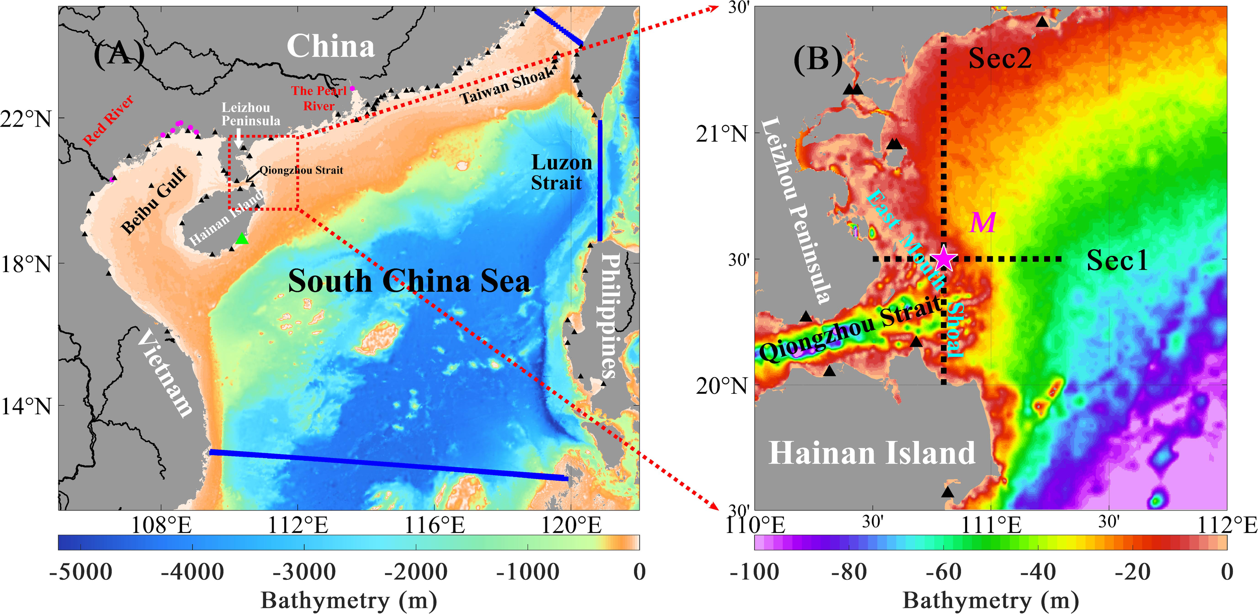
Figure 1. (A) Bathymetry (m) in the northern and central SCS. Pink dots mark the locations of eight rivers entering the northern SCS, namely, the Pearl River, Nanliu River, Dafeng River, Qin River, Maoling River, Fangcheng River, Beilun River, and Red River, from east to west. Black triangles denote the locations of 78 tide gauge stations in the coastal areas of the northern SCS and the green triangle denotes the submarine cable real-time observation station in the southeastern coastal waters of the Hainan Island. The blue solid lines represent the three open boundaries for the model domain. (B) Bathymetry (m) in the study area. Black triangles denote the locations of nine tide gauge stations in the study area. The pink star denotes 110.80°E, 20.50°N, where the most significant tidal temperature variability occurs in summer, and is marked as M. The zonal and meridional dashed lines denote Sec1 and Sec2, which intersect at M.

In the literature, there have been many studies revealing the significant tidal variabilities and associated spring-neap cycles of the physical-biogeochemical conditions in the northern SCS, especially near oceanic fronts in large river estuaries, based on observations, numerical simulations, and data assimilation (Liu et al., 2020; Yan et al., 2020; Yang et al., 2022; Zhi et al., 2022). The underlying mechanisms primarily include tidal current advection and tide-induced turbulent mixing, both of which play essential roles in the three-dimensional transports of energy and materials within the shelf seas (Yu et al., 2022; Wu et al., 2025). Coastal upwelling is also observed to occur frequently in the northern SCS, bringing cold and nutrient-rich waters upward from the sea bottom to the sea surface and thus greatly influencing the regional climate and marine ecosystem (Jing et al., 2009; Hu and Wang, 2016; Lao et al., 2022). Coastal upwelling in the northern SCS is largely controlled by topographic features, tidal forcing, river discharges, and sea surface wind forcing (Jing et al., 2009; Gan et al., 2009; Wang et al., 2014, 2015; Li et al., 2020).

Previous studies have greatly advanced our knowledge of the dynamics of tidal variability and coastal upwelling in the northern SCS. Particularly, many studies proved that tidal forcing could greatly affect the complex three-dimensional coastal upwelling dynamics (Lü et al., 2008; Lin and Gan, 2024). However, whether coastal upwelling can modulate tidal variability or not is still unknown. Recently, we found that coastal upwelling can cause significant synoptic-to-intraseasonal variations in tidal temperature variability near a strong shelf front east of the Leizhou Peninsula and Qiongzhou Strait in the summer. With observations and high-resolution numerical simulations, the objectives of the current study are to document in detail the synoptic-to-intraseasonal variations in tidal temperature variability caused by coastal upwelling east of the Leizhou Peninsula and Qiongzhou Strait and clarify the underlying dynamics. The rest of the paper is organized as follows. Section 2 presents the data, model configuration, and methodology. Section 3 presents the seasonal and synoptic-to-intraseasonal variations in tidal temperature variability east of the Leizhou Peninsula and Qiongzhou Strait derived from the numerical simulation. Section 4 investigates the underlying dynamics. Section 5 provides a brief summary.

2 Data, model configuration and methodology

2.1 Observations

We adopted bottom layer temperatures (BLTs) and water depths obtained by a submarine cable real-time observation system (SCROS) to validate the model’s results. The SCROS has been deployed in the marine ranching area around Zhouzai Island since 2022, which is located in the eastern coastal areas of Hainan Island (green triangle in Figure 1A). The SCROS is located at the sea bottom and continuously measures bottom water temperature, salinity, and depth with a 5-min time interval using a HydroCAT conductivity-temperature-depth-oxygen recorder (Zhai et al., 2020, 2021). The submarine cable real-time observations in the coastal waters of Hainan Island are from February 2022 to June 2023.

Harmonic constants of four main tidal constituents O₁, K₁, M₂, and S₂ at 78 tidal gauge stations (black triangles in Figure 1A) in the northern SCS were gathered from previous studies (e.g., Shi et al., 2002; Zu et al., 2007; Chen et al., 2009) and compared with those derived from the model’s results.

In addition, we used sea surface temperatures (SSTs) observed by a moderate-resolution imaging spectroradiometer (MODIS) to validate the model’s outputs and examine the spatiotemporal variations in surface layer thermal fronts. The daily SST data were downloaded from the OceanColor website. The MODIS SST has a horizontal resolution of approximately 4 km and spans from July 2002 to the present.

2.2 Model configurations

The Semi-implicit Cross-scale Hydroscience Integrated System Model (SCHISM) was employed to conduct the numerical simulation. SCHISM is a three-dimensional semi-implicit cross-scale modeling system developed based on a Semi-implicit Eulerian-Lagrangian Finite Element (Zhang and Baptista, 2008; Zhang et al., 2016). It employs unstructured grids and utilizes a semi-implicit finite element/finite volume method along with a semi-implicit time discretization method to solve the Navier–Stokes equations. SCHISM can perform efficient and accurate numerical simulations in regions with complex coastlines and topography (Wu et al., 2023a; Yan et al., 2024; Hu L. Y. et al., 2024). Additionally, SCHISM provides localized sigma coordinates with shaved cells for a vertical coordinate system, which combines the advantages of traditional z coordinates and terrain-following coordinates, thereby improving the simulation of bottom layer processes (Zhang et al., 2015).

The model domain covers the northern and central SCS, extending zonally from 105.1°E to 121.7°E and meridionally from 11.4°N to 25.4°N (Figure 1A). The coastline data were derived from global self-consistent, hierarchical, high-resolution geography data. The horizontal grid size was set to 1–2 km in coastal and reef regions to better simulate the hydrodynamics. It gradually increased seaward and was approximately 20 km in the offshore deep ocean. The entire model domain contained 73,336 nodes and 142,948 grid elements. Localized sigma coordinates with shaved cells were employed for the vertical coordinate system. There were 21 layers in the coastal areas shallower than 50 m and up to 51 layers in offshore areas deeper than 50 m. The bathymetry data were interpolated from the Shuttle Radar Topography Mission 15Plus V2.1 (Tozer et al., 2019).

The initial and boundary conditions for the model were interpolated from the global 1/12° reanalysis data with 41 layers prepared with the Hybrid Coordinate Ocean Model and Navy Coupled Ocean Data Assimilation. Harmonic constants of eight major tidal constituents (M₂, S₂, N₂, K₂, K₁, P₁, O₁, and Q₁) were extracted from the global ocean tidal atlases of Finite Element Solution 2014 (Lyard et al., 2021) and were applied to the model for tidal forcing. To improve the simulation accuracy, eight major rivers were considered in the model, namely the Pearl River, Nanliu River, Qin River, Fangcheng River, Dafeng River, Maoling River, Beilun River, and Red River. Climatological monthly mean values of the rivers’ runoff were used in the model (Wu et al., 2023b). In the river estuaries, the temperature was obtained from the MODIS climatological mean SST, and salinity was set to 5 PSU (Wu et al., 2023a). Hourly atmospheric variables forcing the model at the sea surface came from the fifth generation of the global reanalysis dataset of the European Centre for Medium-Range Weather Forecasts (ERA5; Wu et al., 2020).

The numerical simulation spans the period from 1 October 2020 to 29 February 2024 with a time step of 120 s. Hourly results were output and analyzed.

2.3 Statistical parameters

For two time series (or spatial maps) of x and y, we calculated four statistical parameters, namely the correlation coefficient (CC), mean absolute error (MAE), root mean square error (RMSE), and agreement index (Skill). Their definitions are presented as follows

$\begin{array}{ll}\begin{array}{c}CC=\frac{{\sum }_{i=1}^n(x_i-\langle x\rangle )(y_i-\langle y\rangle )}{\sqrt{{\sum }_{i=1}^n{(x_i-\langle x\rangle )}^2·{\sum }_{i=1}^n{(y_i-\langle y\rangle )}^2}}\end{array}& (1)\end{array}$

$\begin{array}{ll}\begin{array}{c}MAE=\frac{{\sum }_{i=1}^n\left|x_i-y_i\right|}{n}\end{array}& (2)\end{array}$

$\begin{array}{ll}\begin{array}{c}RMSE=\sqrt{\frac{{\sum }_{i=1}^n{(x_i-y_i)}^2}{n}}\end{array}& (3)\end{array}$

$\begin{array}{ll}\begin{array}{c}Skill=1-\frac{{\sum }_{i=1}^n{(x_i-y_i)}^2}{{\sum }_{i=1}^n{(\left|x_i-\langle y\rangle \right|+\left|y_i-\langle y\rangle \right|)}^2}\end{array}& (4)\end{array}$

In Equations 1–4, x_i and y_i represent the simulated and observed values, respectively. The n is the number of time moments (or grid points) and $\langle \rangle$ denotes the mean value over all the time moments (or grid points). In the current study, the linear correlation coefficients are all above the 95% confidence level unless otherwise specified.

2.4 Temperature budget equation

The temperature budget equation at any grid point (x, y, z) is written as

$\begin{array}{ll}\begin{array}{c}\underset{RATE}{\underbrace{\frac{\partial T}{\partial t}}}=\underset{ADV}{\underbrace{-\left(u\frac{\partial T}{\partial x}+v\frac{\partial T}{\partial y}+w\frac{\partial T}{\partial z}\right)}}+\underset{VDIF}{\underbrace{\frac{\partial (K_V\frac{\partial T}{\partial z})}{\partial z}}}+D_h\end{array}& (5)\end{array}$

with the following surface and bottom boundary conditions

$\begin{array}{ll}\begin{array}{c}{(K_V\frac{\partial T}{\partial z})}_{z=0}=\frac{Q_{net}}{{\rho }_0{C}_p}\end{array}& (6)\end{array}$

$\begin{array}{ll}\begin{array}{c}{(K_V\frac{\partial T}{\partial z})}_{z=-h}=0\end{array}& (7)\end{array}$

In Equations 5–7, T, h, ρ₀, and C_p represent water temperature, depth, mean density (1,025 kg·m⁻³), and specific heat capacity at constant pressure (4,007 J·kg⁻¹·°C⁻¹), respectively. u, v, and w are the zonal, meridional, and vertical velocities, respectively. Q_net is the net sea-air heat flux. K_V is the vertical turbulence-induced heat diffusivity. RATE denotes the total temperature change rate. ADV represents the temperature change rate caused by three-dimensional current transport, and VDIF represents the temperature change rate caused by turbulence-induced vertical diffusion. D_h is the temperature change rate caused by horizontal diffusion. The contribution of D_h is two to three orders of magnitude smaller than that of ADV and thus is disregarded here. The depth-averaged temperature budget equation at any grid point (x, y) can then be written as Equation 8

$\begin{array}{ll}\overline{RATE}=\overline{ADV}+\overline{SHF}& (8)\end{array}$

where the overbar $‾$ denotes the vertical average over the whole water column and $\overline{SHF}=Q_{net}/({\rho }_{0}h{C}_p)$.

2.5 Magnitude of tidal temperature variability

As illustrated in the following sections, seawater temperature in the study area displays multi-scale variabilities. Within 1 lunar day, temperature is usually dominated by tidal variability. However, the magnitude of tidal temperature variability exhibits significant synoptic-to-intraseasonal variations. In some days, temperature shows no significant tidal variability. In the current study, the diurnal standard deviation (STD) of hourly temperature was used to quantify the magnitude of tidal temperature variability and is calculated as follows. For each lunar day, 24 hours of hourly temperature are first detrended to exclude subtidal signals. The resultant hourly temperature anomalies (T′) in that lunar day are then used to calculate the diurnal standard deviation following $\sqrt{\raisebox{1ex}{${\sum }_{i=1}^n{(T{\text{'}}_i-T\text{'})}^2$}\!\left/ \!\raisebox{-1ex}{$n-1$}\right.}$, where n=24. Note that one can obtain nearly the same results with 25 hours (n=25) of hourly temperature for 1 lunar day.

3 Tidal temperature variability

3.1 Comparison of numerical simulation with observations

We compared the observed harmonic constants of the four tidal constituents with the model results at the tidal gauge stations (Figures 2A, B). The correlation coefficients for the amplitudes of the O₁, K₁, M₂, and S₂ tidal components were 0.98, 0.95, 0.99, and 0.97 between the observations and the model’s results, and those for the phases of the O₁, K₁, M₂, and S₂ tidal components were 0.99, 0.99, 0.99 and 0.98 between the observations and the model’s results. The mean absolute errors for the amplitudes of the O₁, K₁, M₂, and S₂ tidal components were 0.06 m, 0.06 m, 0.06 m, and 0.03 m between the observations and the model’s results, and those for the phases of the O₁, K₁, M₂, and S₂ tidal components were 5.85°, 9.91°, 12.19°, and 16.29° between the observations and the model’s results. The root mean square errors for the amplitudes of the O₁, K₁, M₂, and S₂ tidal components were 0.10 m, 0.08 m, 0.08 m, and 0.03 m between the observations and the model’s results, and those for the phases of the O₁, K₁, M₂, and S₂ tidal components were 8.84°, 11.96°, 16.83° and 21.22° between the observations and the model’s results. The above statistical parameters indicate that the simulated tidal harmonic constants agree with the observations for all the four main tidal constituents at most stations.

Figure 2

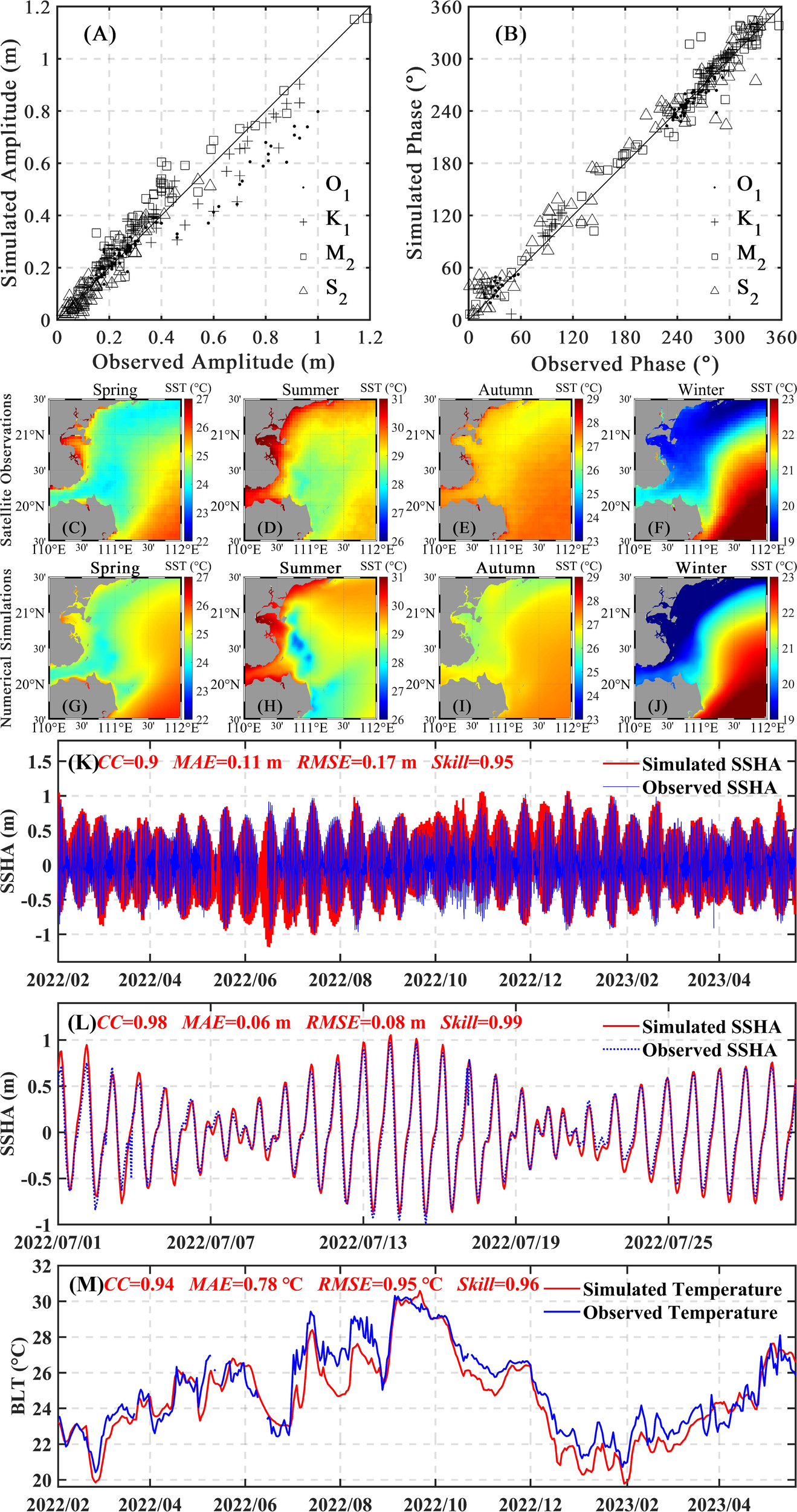
Figure 2. Comparison of observations and numerical simulation. (A) Observed and simulated amplitudes of O₁, K₁, M₂, and S₂ tidal constituents at tidal gauge stations in coastal areas of the northern SCS. (B) Same as (A) but for observed and simulated tidal phases. (C–F) Three-year (March 2021–February 2024) mean satellite-observed SST (°C) in the study area in spring, summer, autumn, and winter. (G–J) Same as (C–F) but for model-simulated SST (°C). (K) SCROS-observed and model-simulated hourly sea surface height anomaly (SSHA, m) in the southeastern coastal waters of Hainan Island from February 2022 to June 2023. (L) Same as (K) but in July 2022. (M) Same as (K) but for daily BLT (°C) from February 2022 to June 2023.

We further compared the 3-year (March 2021–February 2024) mean SST in satellite observations and model simulations in the four seasons (Figures 2C–J). The numerical simulation accurately reproduced the satellite-observed seasonal variations in SST in the SCS, with spatial correlation coefficients ranging from 0.64 in autumn to 0.90 in winter and agreement indices ranging from 0.65 in autumn to 0.92 in winter between them. Especially in summer, the model’s results show two low SST centers around 20.5°N, similar to the satellite observations.

In addition, we also compared the SCROS-observed and model-simulated hourly sea surface height anomaly (SSHA) and BLT in the southeastern coastal waters of Hainan Island. The SCROS-observed hourly SSHA and model-simulated hourly SSHA showed a high correlation coefficient of 0.90 and agreement index of 0.95 but relatively low mean absolute error of 0.11 m and root mean square error of 0.17 m during the SCROS observation period of February 2022 to May 2023 (Figure 2K). Figure 2L presents the tidal variations in hourly SSHAs in both the SCROS observations and the numerical simulation in July 2022, which agree with each other, showing a high correlation coefficient of 0.98 and agreement index of 0.99 but low mean absolute error of 0.06 m and root mean square error of 0.08 m. The SCROS-observed daily BLT and model-simulated daily BLT also agree with each other, with a high correlation coefficient of 0.94 and agreement index of 0.96 but low mean absolute error of 0.78°C and root mean square error of 0.95°C (Figure 2M).

The above comparisons confirm that our numerical simulation captures well both the tidal and subtidal variations in the hydrodynamics in the coastal waters of the northern SCS.

3.2 Seasonal temperature variations

Figure 3 shows the three-dimensional structure of the 3-year seasonal mean temperature in the study area. In spring, SST remains relatively uniform in space, ranging from 23°C to 27°C (Figure 3A). It increases significantly from spring to summer, exceeding 30°C in the coastal regions and with a cold center to the east of the Leizhou Peninsula (Figure 3B). It begins to decrease in autumn (Figure 3C) and reaches its lowest values in winter, ranging from 18°C to 23°C (Figure 3D). Due to the shallow water depths in the coastal areas, BLT basically agrees with SST, being warmer in summer and cooler in winter (Figures 3E–H). However, SST and BLT experience quite different spatiotemporal variations in their horizontal gradients. To the east of the Leizhou Peninsula, significant SST gradients appear in both summer and winter. The large SST gradient in summer is basically located close to the east coast of the Leizhou Peninsula and should be related to the existence of the surface cold center. The large SST gradient in winter is located far away from the east coast of the Leizhou Peninsula and forms a strong ocean front to separate offshore warm waters from nearshore cold waters (Figures 2F, G, 3D; Wang et al., 2001). In contrast, significant BLT gradients only appear in summer and are much stronger than SST gradients. They form a strong ocean front located close to the east coast of the Leizhou Peninsula and east entrance of the Qiongzhou Strait.

Figure 3

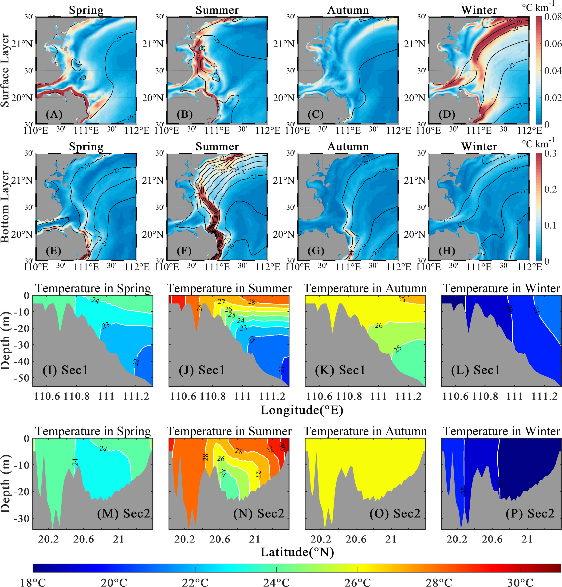
Figure 3. Three-dimensional structure of the 3-year seasonal mean temperature (°C) in the study area from the numerical simulation. (A–D) SST (contour) and its horizontal gradient (°C km^–1; color) in spring, summer, autumn, and winter, respectively. (E–H) Same as (A–D) but for BLT (contour) and its horizontal gradient (°C km^–1; color). (I–L) Same as (A–D) but for temperature at Sec1 to the east of the Leizhou Peninsula. (M–P) Same as (A–D) but for temperature at Sec2 to the east of the Leizhou Peninsula.

Figures 3I–P further show the 3-year seasonal mean temperature along two sections to give more detail of the three-dimensional temperature structure in regions between the east coast of the Leizhou Peninsula and the strong winter offshore SST front. As displayed in Figure 1B, Sec1 extends zonally along 20.5°N from the east coast of the Leizhou Peninsula at 110.5°E to offshore areas at 111.3°E, and Sec2 extends meridionally along 110.8°E from the northeast coast of Hainan Island at 20.0°N to 21.4°N. Sec1 and Sec2 intersect at 110.8°E, 20.5°N, where the most significant tidal temperature variability exists, as will be shown in the following subsection. The most striking feature in Figures 3I–P is the coexistence of the pronounced ocean thermal front and stratification below the sea surface layer in summer. The significant ocean thermal front is located on the sea floor slope, where the topography changes dramatically from nearshore regions to offshore regions (Figures 1B, 3J; Bai et al., 2020). It is formed primarily due to the enhanced solar radiation and tidal mixing, with possibly secondary contributions from sea surface winds (Simpson and Bowers, 1981; Bai et al., 2020; Wu et al., 2023b). Isotherms above the deep ocean fronts are shallower than those in the offshore regions, indicating the upwelling of cold waters, which subsequently forms the surface cold center and results in large SST gradients to the west, as seen in Figure 3B. In contrast, the water column is well-mixed vertically in winter, resulting in the disappearance of ocean thermal stratification.

3.3 Seasonal variations in tidal temperature variability

Figures 4A–H show the seasonal mean diurnal standard deviation of hourly temperature in the sea surface and bottom layers in the four seasons. First, tidal temperature variability is generally stronger in the bottom layer than in the surface layer in all four seasons. Second, the seasonal mean diurnal standard deviation of hourly temperature is largest in summer (~0.93°C), followed by spring (<0.40°C), and is smallest in autumn and winter (<0.30°C) in both the surface and bottom layers. Third, large values of summer mean diurnal standard deviation of SST and BLT only exist in a narrow band extending from 110.5°E to 111°E in the zonal direction and from 20°N to 21.2°N in the meridional direction in shallow waters (<40 m) to the east of the Leizhou Peninsula and Qiongzhou Strait. The most pronounced tidal temperature variability occurs at 110.80°E, 20.50°N (M; the pink star in Figures 1B, 4) to the southeast of the Leizhou Peninsula.

Figure 4

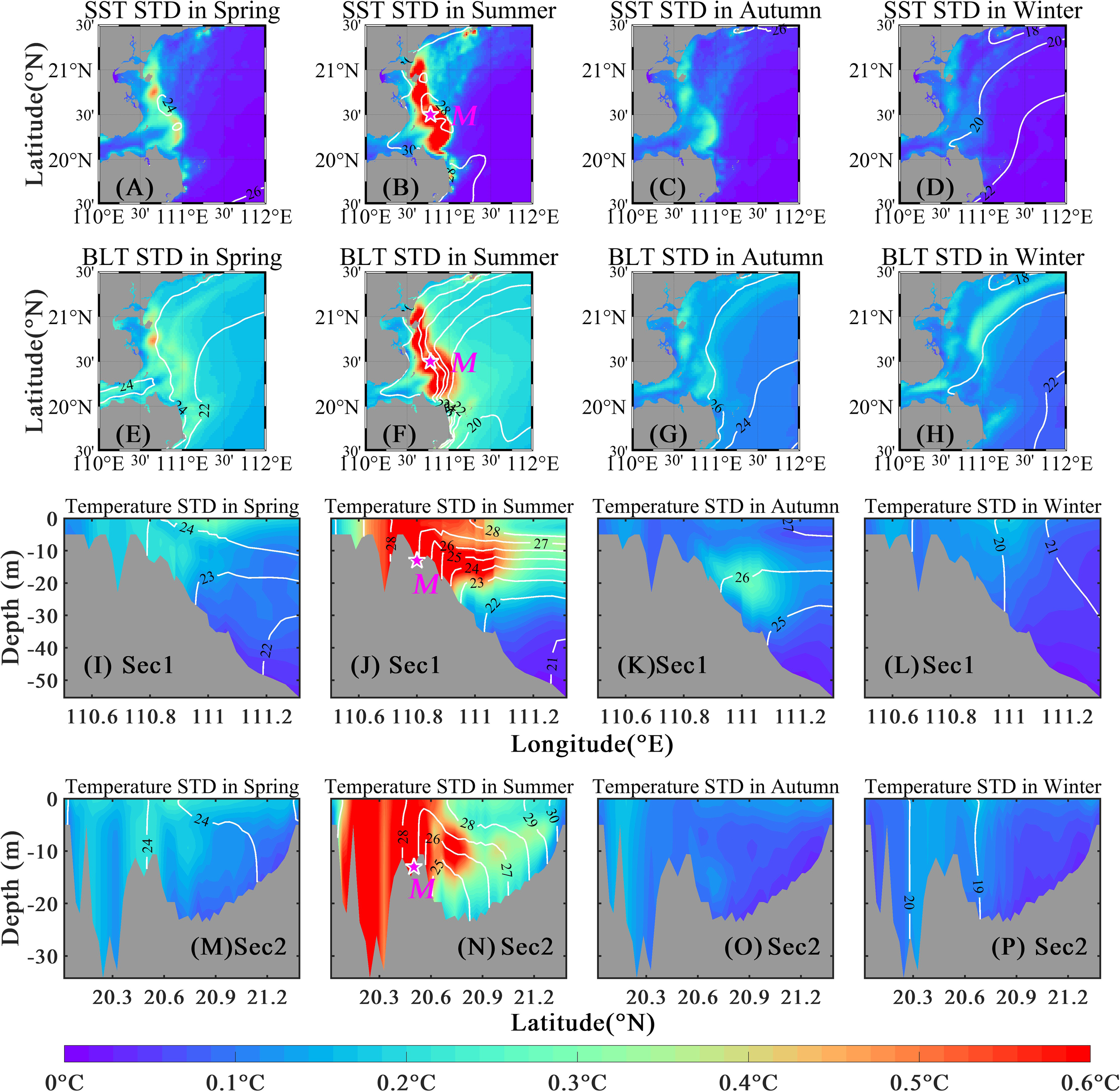
Figure 4. Three-dimensional structure of the 3-year seasonal mean diurnal standard deviation of hourly temperature (°C) from the numerical simulation. (A) Diurnal standard deviation (color) and 3-year mean (contour) of hourly SST in spring. (B) Same as (A) but in summer. (C) Same as (A) but in autumn. (D) Same as (A) but in winter. (E–H) Same as (A–D) but for hourly BLT. (I–L) Same as (A–D) but for the temperature at Sec1. (M–P) Same as (A–D) but for the temperature at Sec2. In (B, F, J, N), the pink stars denote the horizontal position at 110.80°E, 20.50°N (M).

We further examined the seasonal mean diurnal standard deviation of hourly temperature along Sec1 and Sec2 to provide more insights into the three-dimensional structure of tidal temperature variability (Figures 4I–P). As clearly seen in Figure 4, tidal temperature variability is much stronger throughout the water column in summer than in other seasons. In summer, tidal temperature variability is largest in the bottom layer and weakens upward to the sea surface. Horizontally, strong tidal temperature variability mainly occurs on the landward side of the offshore thermal front (Figures 4F, J). This finding suggests that the spatiotemporal variations in tidal temperature variability in the study area should be closely related to activities of ocean thermal fronts, and the detailed underlying dynamics will be discussed in Section 4.

3.4 Tidal temperature variability in summer

The above results indicate that tidal temperature variability is strongest in summer. Thus, one important question is whether the magnitude of tidal temperature variability in summer remains unchanged or varies significantly with time. For that purpose, Figure 5A compares the hourly time series of SST and BLT at M in the summers of 2021–2023, which are essentially equal to each other. Spectral analyses of hourly time series of SST and BLT indicate that both SST and BLT are dominated by tidal variability within 1 lunar day. Unexpectedly, tidal variabilities of both SST and BLT exhibit strong synoptic-to-intraseasonal variations, being significant on some days but insignificant on other days. To clearly see this, we show in Figure 5A the daily time series of diurnal standard deviation of hourly BLT (black dashed line), which is nearly the same as that of hourly SST. The diurnal standard deviation of hourly BLT exhibits strong synoptic-to-intraseasonal variations with a large range of 0°C–2.36°C. Synoptic-to-intraseasonal variations in the magnitude of tidal temperature variability have no predominant periods and are quite different from the spring-neap variability.

Figure 5

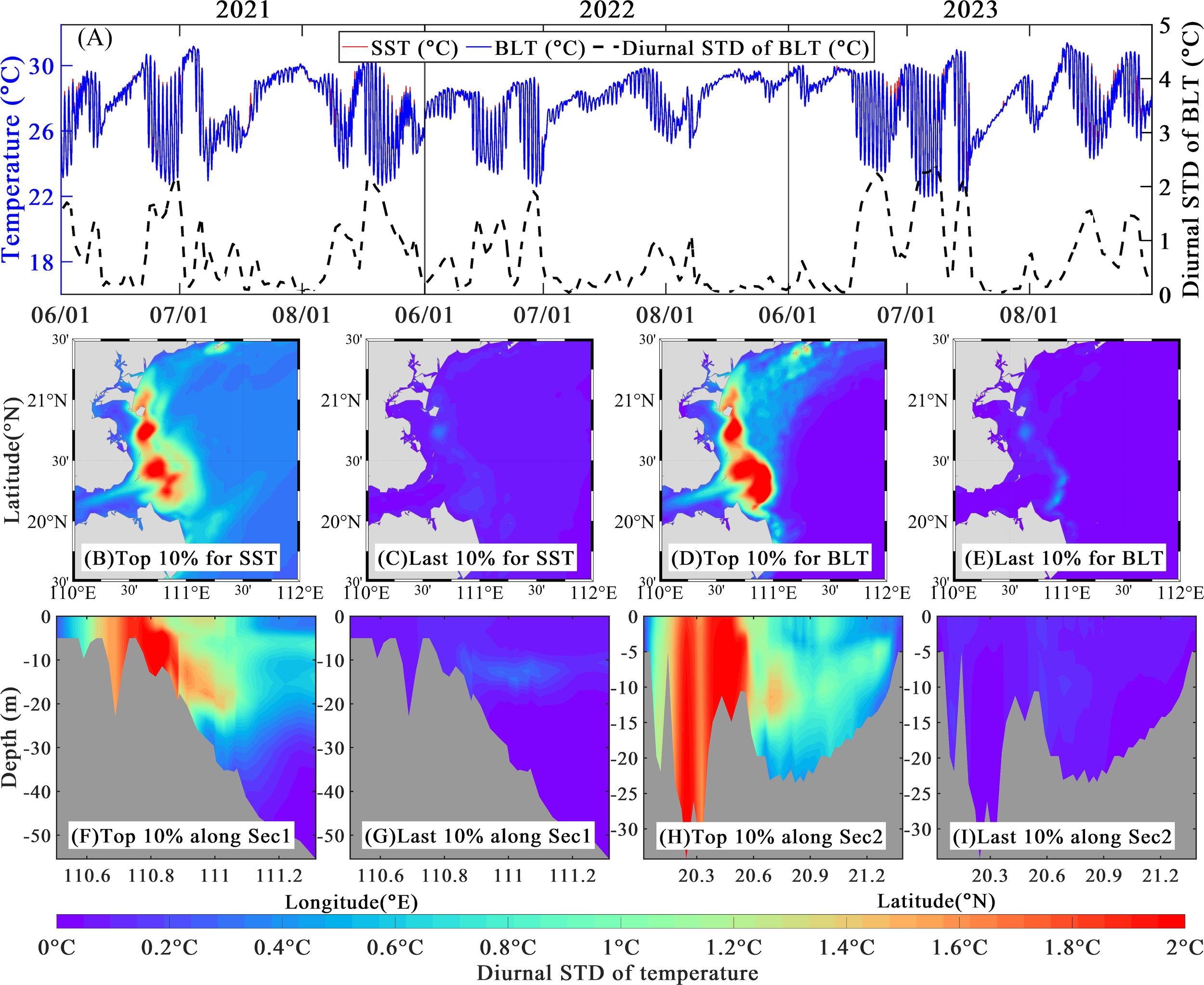
Figure 5. Synoptic-to-intraseasonal variations in the magnitude of tidal temperature variability during the summers of 2021–2023. (A) Hourly SST (°C, red line), hourly BLT (°C, blue line) and its diurnal standard deviation (black dashed line) at M. (B) Spatial distribution of the top 10% diurnal standard deviation of hourly SST in the summer of 2021. (C) Spatial distribution of the last 10% diurnal standard deviation of hourly SST in the summer of 2021. (D–E) Same as (B, C) but for BLT. (F–I) Same as (B–E) but for diurnal standard deviation of hourly temperature at Sec1 and Sec2 to the east of the Leizhou Peninsula.

To give more details on the three-dimensional structure of synoptic-to-intraseasonal variations in tidal temperature variability, we calculated the top 10% and last 10% of the diurnal standard deviation of hourly temperature in the summer of 2021 and display the results in Figures 5B–I. Similar results were obtained in the summers of 2022–2023 (Figure not shown). The most notable feature is that synoptic-to-intraseasonal variations in tidal temperature variability also vary in magnitude significantly with space. The top 10% diurnal standard deviations of hourly BLT and SST share similar spatial distributions to seasonal mean diurnal standard deviations of hourly BLT and SST (Figures 4B, F). Note that the top 10% diurnal standard deviation of hourly BLT is generally larger than that of hourly SST, further proving stronger tidal temperature variability in the bottom layer than in the surface layer. Large values (1°C–2°C) of the top 10% diurnal standard deviations of both hourly BLT and SST are concentrated in the same narrow band in shallow waters to the east of the Leizhou Peninsula and Qiongzhou Strait to the seasonal mean diurnal standard deviations (Figures 4B, F). In contrast, the last 10% diurnal standard deviation of hourly temperature is universally small (<0.2°C) over the entire study area, showing much smaller spatial difference than the top 10% diurnal standard deviation of hourly temperature. The detailed vertical structure of synoptic-to-intraseasonal variations in tidal temperature variability can be clearly seen from the top 10% and last 10% diurnal standard deviations of hourly temperature along Sec1 and Sec2. Overall, synoptic-to-intraseasonal variations in tidal temperature variability decrease in magnitude upward from the sea bottom to the sea surface.

The above results highlight the significant synoptic-to-intraseasonal variations in the magnitude of tidal temperature variability in shallow shelf waters to the east of the Leizhou Peninsula and Qiongzhou Strait in the summer.

4 Mechanisms

4.1 Diurnal variations in tidal currents and horizontal temperature gradient

In this section, temperature budget analyses are presented to identify the underlying dynamics controlling tidal temperature variability in the study area in the summers of 2021−2023. For that purpose, we calculated the depth-averaged temperature budget terms over the whole water column at each grid point in the study area. Figure 6A shows the hourly time series of the depth-averaged temperature budget terms at M. The most prominent feature is that $\overline{RATE}$ equals $\overline{ADV}$, especially in days when tidal temperature variability is significant. The agreement index between hourly time series of $\overline{RATE}$ and $\overline{ADV}$ in the summers of the three years is approximately 0.99. As an example, Figure 6B shows the hourly time series of the depth-averaged temperature budget terms at M on 25 June 2021, and one can see that $\overline{RATE}$ is predominantly controlled by $\overline{ADV}$.

Figure 6

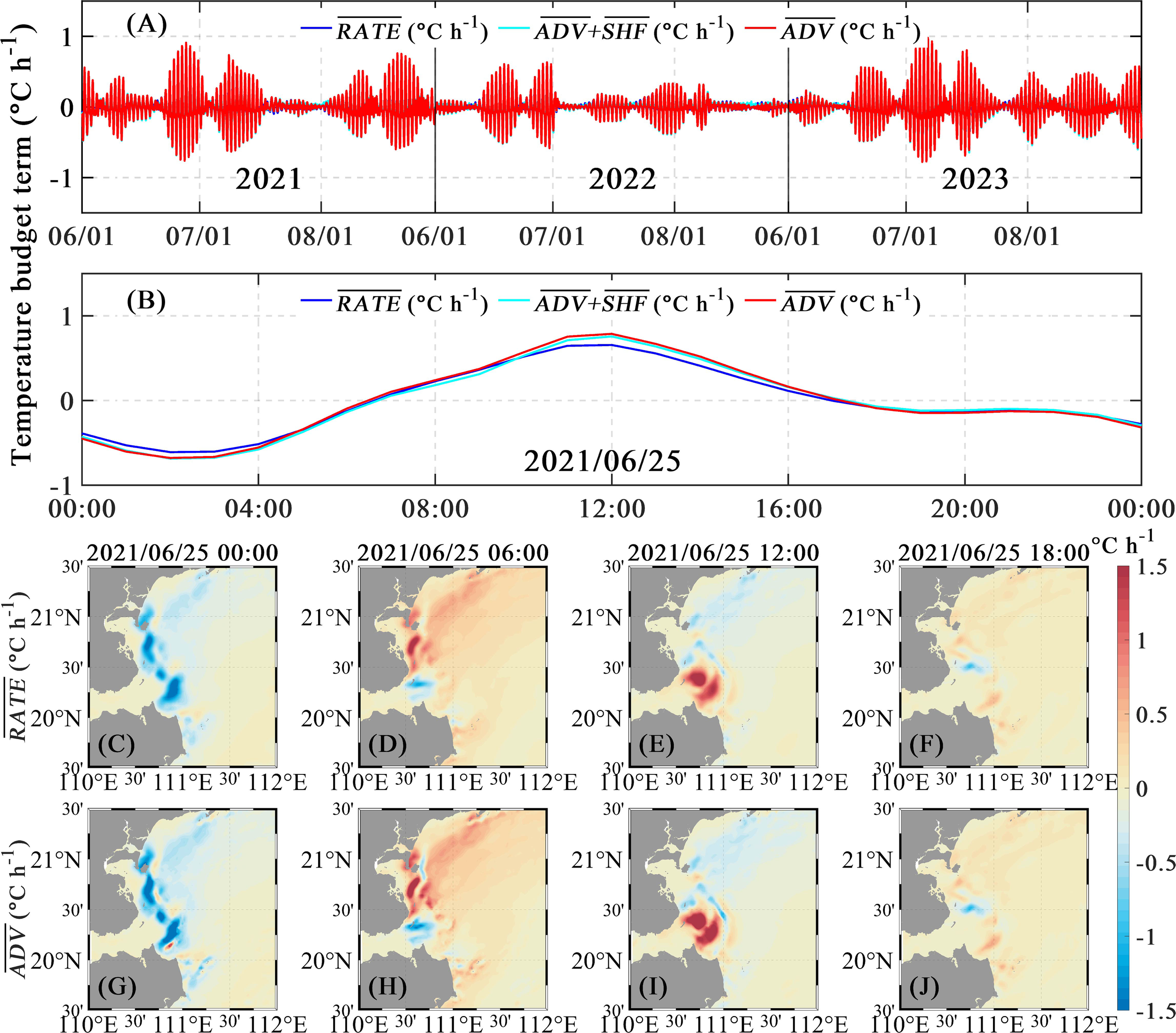
Figure 6. (A) Hourly time series of depth-averaged temperature budget terms (°C h^–1) at M in the summers of 2021–2023. (B) Hourly time series of depth-averaged temperature budget terms (°C h^–1) on 25 June 2021. (C–F) Six-hourly maps of depth-averaged temperature change rate ($\overline{RATE}$, °C h^–1) on June 25, 2021. (G–J) Same as (C–F) but for depth-averaged current heat transport ($\overline{ADV}$, °C h^–1).

In addition, we also examined the spatial distributions of temperature budget terms at different time points in 1 day. Figures 6C–F display the 6-hourly maps of $\overline{RATE}$, which basically equal to $\overline{ADV}$ (Figures 6G–J) over the whole study area. The above findings indicate that tidal temperature variability in the study area is predominantly controlled by current heat transport, while the contributions of air-sea heat exchange can be disregarded.

Current heat transport is the product of current velocity and horizontal temperature gradient. Therefore, it is useful to examine whether there are synoptic-to-intraseasonal variations in magnitudes of hourly current and horizontal temperature gradient. As an example, Figures 7A, B show hourly time series of SSHA and bottom current velocity at M during the summer of 2021. As clearly seen from the figure, both SSHA and bottom currents are dominated by tidal dynamics within 1 lunar day and their magnitudes exhibit significant spring-neap cycles. One can obtain similar results in the summers of 2022–2023. This finding strongly indicates that tidal currents experience no synoptic-to-intraseasonal variations in the summer, and therefore are not responsible for the synoptic-to-intraseasonal variations in the magnitude of tidal temperature variability in the study area in the summer.

Figure 7

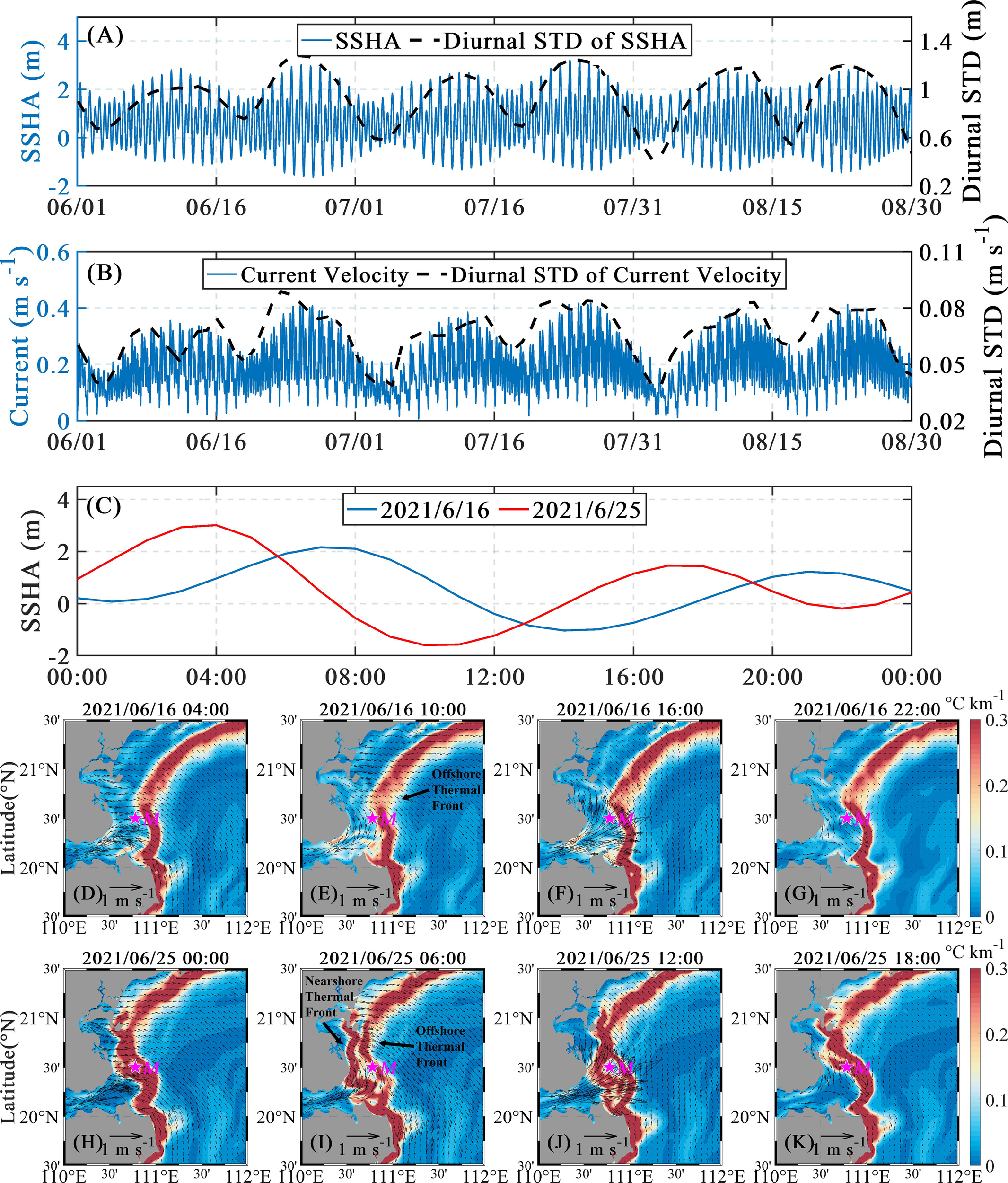
Figure 7. (A) Hourly SSHA (m) and its diurnal standard deviation at M during the summer of 2021. (B) Hourly bottom current velocity (m s^–1) and its diurnal standard deviation at M during the summer of 2021. (C) Hourly SSHA (m) at M on 16 and 25 June 2021. (D–G) Six-hourly maps of tidal current vector (arrow; m s^–1) and horizontal temperature gradient (color; °C km^–1) in the bottom layer on 16 June 2021, when tidal temperature variability is weak. (H–K) Same as (D–G) but on 25 June 2021, when tidal temperature variability is strong.

Based on the above results, we hypothesize that the horizontal temperature gradient should play a dominant role in generating synoptic-to-intraseasonal variations in the magnitude of tidal temperature variability. To gain more insight into the underlying dynamics, we analyzed the hourly evolution of tidal current vector and horizontal BLT gradient on 16 and 25 June 2021 in detail. As shown in Figure 5A, tidal temperature variability is quite weak on 16 June, but is very strong on 25 June. Figure 7C shows that hourly SSHA on the two days displays significant and comparable tidal variations, quite different from hourly temperature (Figure 5A).

Figures 7D–K then give the 6-hourly maps of hourly tidal current vector and horizontal BLT gradient during flood tides and ebb tides on the 2 days. Note that in the whole study period, tidal current vectors and BLT fronts show similar hourly variations in days with weak tidal temperature variability to those on 16 June but show similar hourly variations in days with strong tidal temperature variability to those on 25 June. Both flood currents and ebb currents have similar magnitudes and spatial distributions on the 2 days. However, the horizontal BLT gradient shows quite different spatiotemporal variations on the 2 days. On 16 June, there is only the offshore BLT front extending along the topographic contours on the sea floor slope. This offshore BLT front experiences no significant changes during the tidal cycles. Therefore, horizontal BLT gradients in the nearshore regions are nearly zero and thus lead to insignificant tidal temperature variability. In contrast, horizontal BLT gradients experience more complicated changes on 25 June. First, the offshore BLT front on the sea floor slope moves much closer to the coastline in the north. Second, there is another BLT front in the nearshore region between the coastline and the offshore BLT front on the sea floor slope. The nearshore BLT front is mainly south of 21.2°N, with a much shorter length than the offshore BLT front, and swings back and forth in the directions of tidal current vectors.

The above findings strongly suggest that significant tidal temperature variability is dynamically related to the formation and tidal current-induced swinging of the nearshore temperature front. From this, one can also easily understand that the significant tidal temperature variability is concentrated in a narrow band south of 21.2°N (Figures 4, 5) because the nearshore BLT front occurs south of 21.2°N (Figures 7H–K).

4.2 Synoptic-to-intraseasonal variations in ocean thermal fronts

In addition to diurnal variations, the above results also suggest that strong synoptic-to-intraseasonal variations in the magnitude of tidal temperature variability in the study area in the summer are dynamically caused by strong synoptic-to-intraseasonal variations in the nearshore thermal front. Therefore, exploring the dynamics for the synoptic-to-intraseasonal variations in tidal temperature variability becomes equivalent to clarifying the causes for the synoptic-to-intraseasonal variations in the nearshore thermal front. For that purpose, we calculated the correlation coefficients of the diurnal standard deviation of hourly BLT at M with daily BLT and daily BLT gradient. As shown in Figure 8A, the correlation coefficients between the diurnal standard deviation of hourly BLT at M and daily BLT gradient are widely positive in the nearshore regions between the coastline and offshore thermal front. The positive correlation coefficient is largest in a narrow southeast-northwest band (correlation coefficient=0.8–0.91; region G in Figure 8A) adjacent to M.

Figure 8

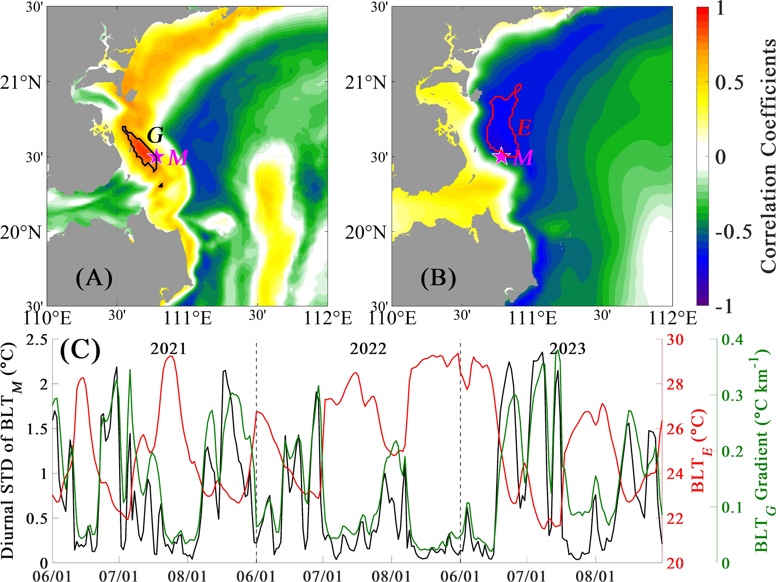
Figure 8. Relationship between the synoptic-to-intraseasonal variations in the magnitude of tidal temperature variability at M and those in BLT and BLT gradient in the summers of 2021–2023. (A) Spatial map of the linear correlation coefficients between the diurnal standard deviation of hourly BLT at M and daily BLT gradient. The black curve marks region G to the east of the Leizhou Peninsula with positive correlation coefficients larger than 0.8 above the 95% confidence level. (B) Spatial map of the linear correlation coefficients between the diurnal standard deviation of hourly BLT at M and daily BLT. The pink curve marks region E to the east of the Leizhou Peninsula with negative correlation coefficients smaller than −0.66 above the 95% confidence level. In (A, B), the pink star indicates the M as shown in Figure 1B. (C) Time series of diurnal standard deviation of hourly BLT at M (BLT_M, °C; black line), daily BLT averaged over region E (BLT_E, °C; red line), and daily BLT gradient averaged over region G (BLT_G, °C km^–1; green line).

As shown in Figure 8B, the correlation coefficients between the diurnal standard deviation of hourly BLT at M and daily BLT are generally positive at the east entrance of the Qiongzhou Strait and in the eastern coastal areas of the Leizhou Peninsula but are more significantly negative in the offshore frontal areas. In particular, there is a meridional band extending northward from M to approximately 21.0°N (region E in Figure 8A) and showing highly negative correlation coefficients of −0.84 to −0.8. To clearly display their relationship, Figure 8C further compares the diurnal standard deviation of hourly BLT at M, daily mean BLT gradient averaged over region G, and daily mean BLT averaged over region E. As expected, the diurnal standard deviation of hourly BLT at M is significantly positively correlated with the daily mean BLT gradient averaged over Region G (correlation coefficient=0.87), which is then significantly negatively correlated with daily mean BLT averaged over region E (correlation coefficient=−0.90).

The above significant correlation coefficients suggest that when region E is occupied by cold (warm) waters, the temperature gradient in region G would be large (small), and the tidal temperature variability at M would be strong (weak). After carefully reviewing the difference in the offshore thermal fronts between 16 and 25 June shown in Figures 7D–K, we speculate that changes in the deep waters in region E are controlled by the zonal movement of the offshore thermal front. In other words, region E would be occupied by cold (warm) waters if the offshore thermal front moves westward close to (eastward away from) the coastline of the Leizhou Peninsula. To verify the above speculation, Figure 9A shows the correlation coefficients between the diurnal standard deviation of hourly BLT at M and daily longitude of the offshore thermal front during the summers of 2021−2023. As expected, the correlation coefficients are significantly negative (−0.65 to −0.6) at latitudes from 20.6°N to 21°N and then decrease in magnitude both northward and southward. This finding suggests that synoptic-to-intraseasonal variations in tidal temperature variability at M should be related to zonal movements of the offshore thermal front within 20.6°N−21°N, which is located to the north of M.

Figure 9

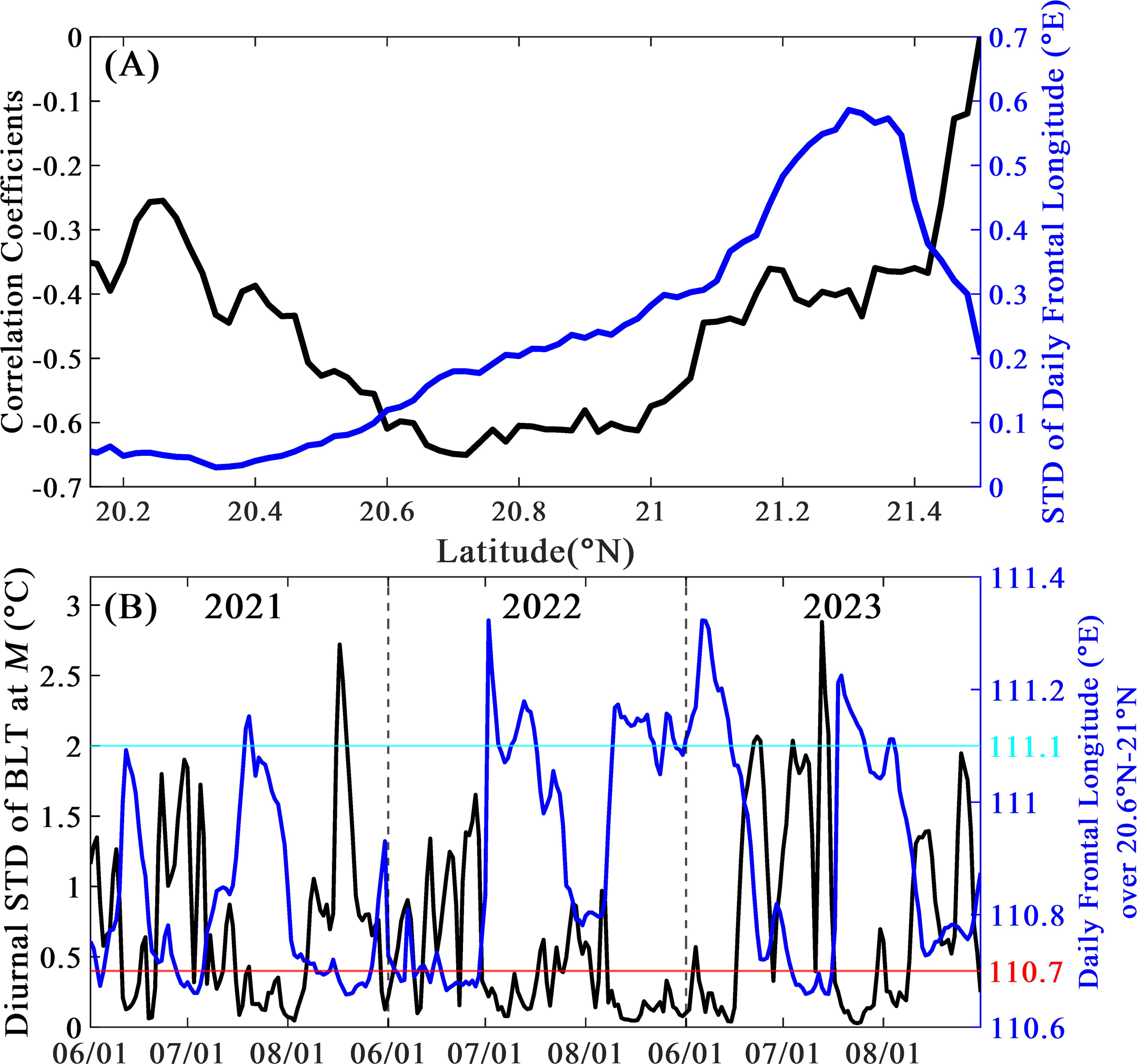
Figure 9. (A) Meridional distributions of the linear correlation coefficients (black line) between the diurnal standard deviation of hourly BLT at M and daily longitude of the offshore thermal front, and standard deviation (blue line) of daily longitude of the offshore thermal front during the summers of 2021−2023. (B) The diurnal standard deviation of hourly BLT at M (black line) and daily longitude of the offshore thermal front averaged within 20.6°N–21°N during the summers of 2021–2023. The red and cyan lines denote daily frontal longitudes at 110.7°E and 111.1°E, respectively.

The standard deviation of daily longitude of the offshore thermal front is nearly zero at the east entrance of the Qiongzhou Strait and gradually increases northward, with its maximum occurring at 21.3°N (Figure 9A). That the zonal swing distance of the offshore thermal front increases northward is quite possibly related to the bottom topography (Figure 1B). At the east entrance of the Qiongzhou Strait, the bottom topography features the East Mouth Shoal and is extremely steep eastward to the deep SCS, which can greatly limit the westward swinging of the offshore thermal front. To the north of the East Mouth Shoal, however, the bottom topography shallows slowly toward the east coast of the Leizhou Peninsula, allowing far-westward moving of the offshore thermal front.

Figure 9B shows the diurnal standard deviation of hourly BLT at M and the daily mean longitude of the offshore thermal front averaged within 20.6°N–21°N to give more details of the temporal variations. The time series of the two variables are significantly correlated with each other with a highly negative correlation coefficient of –0.65. As clearly seen in the figure, the daily mean longitude of the offshore thermal front within 20.6°N–21°N displays significant synoptic-to-intraseasonal variations. A large (small) diurnal standard deviation of hourly BLT at M always corresponds to a small (large) distance between the offshore thermal front and the east coast of the Leizhou Peninsula.

After carefully inspecting Figures 7H–K again, we found that when the offshore thermal front within 20.6°N–21°N moves close to the east coast of the Leizhou Peninsula, the offshore thermal front within 20.35°N–20.6°N in the south becomes more inclined along the southeast-northwest direction and coincides with the north East Mouth Shoal. Strong tidal currents approaching the Leizhou Peninsula in the north and into the Qiongzhou Strait in the south separate the offshore thermal front into two thermal fronts on the south and north sides of the East Mouth Shoal. The thermal front on the south side of the East Mouth Shoal forms the nearshore thermal front and continues to move southwestward under the forcing of tidal currents toward the Qiongzhou Strait. When tidal currents in the Qiongzhou Strait shift eastward, they then push the nearshore thermal front northeastward, which subsequently merges into the offshore thermal front at the East Mouth Shoal. This finding indicates that the formation and synoptic-to-intraseasonal variations of the nearshore thermal front are controlled by zonal swinging of the offshore thermal front within 20.6°N–21°N to the east of the Leizhou Peninsula. That is, significant synoptic-to-intraseasonal variations in tidal temperature variability to the east of the Leizhou Peninsula and Qiongzhou Strait are predominantly caused by synoptic-to-intraseasonal swinging in the zonal direction of the offshore thermal front within 20.6°N–21°N.

4.3 Synoptic-to-intraseasonal variations in coastal upwelling

To further explore the underlying mechanisms for the synoptic-to-intraseasonal variations in the offshore thermal front, we calculated composite maps of sea surface winds, ocean currents, and BLT gradients during two periods when the offshore thermal front within 20.6°N–21°N is east of 111.1°E (Period I, Figure 9B) and west of 110.7°E (Period II, Figure 9B), respectively, in the summers of 2021−2023. As shown in Figure 10, the study area is primarily forced by southerly monsoon winds in the summer. During Period I (Figures 10A–C), southerly winds are weak, and ocean currents in both sea surface and bottom layers are also weak. The reduced ocean dynamics lead to the offshore thermal front being located far away from the Leizhou Peninsula. During Period II (Figures 10D–F), however, southerly winds are strong and generate strong ocean currents in both the surface and bottom layers. In the surface layer, ocean currents are deflected to the right with respect to sea surface wind directions and the angles basically increase from nearshore regions to offshore regions. This finding indicates that sea surface currents are wind-driven Ekman currents in nature. In the bottom layer, ocean currents basically flow northward/northeastward in offshore deep waters but shift to be shoreward in nearshore shallow waters. The shoreward bottom currents then pushed the offshore thermal front moving much close to the Leizhou Peninsula. This kind of vertical structure of ocean currents strongly suggests the existence of significant wind-driven coastal upwelling to the east of the Leizhou Peninsula during Period II.

Figure 10

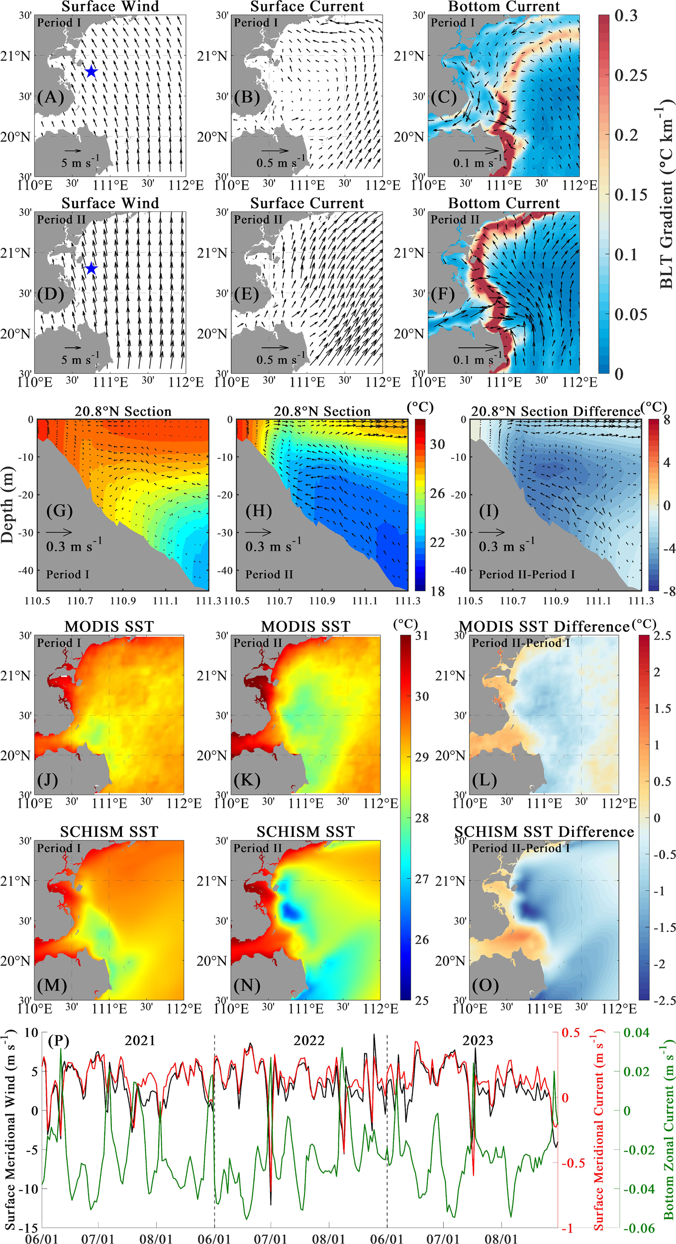
Figure 10. (A) Composite mean 10-m wind vectors (m s⁻¹) during Period I in the summers of 2021−2023. The blue star marks 20.8°N, 110.75°E. (B) Same as (A) but for sea surface current vectors (m s⁻¹). (C) Same as (A) but for bottom current vectors (m s⁻¹, arrows) and BLT gradient (°C km⁻¹, color). (D−F) Same as (A−C) but during Period II in the summers of 2021−2023. (G) Composite mean current vectors (m s⁻¹) and temperature (°C) at 20.8°N to the east of the Leizhou Peninsula during Period I in the summers of 2021−2023. The vertical current component is multiplied by 1,000 for clarity. (H) Same as (G) but during Period II in the summers of 2021−2023. (I) Composite mean current vectors (m s⁻¹) and temperature (°C) at 20.8°N during Period II minus those during Period I. (J) Composite mean SST (°C) during Period I in the summers of 2021–2023 derived from MODIS observations. (K) Same as (J) but during Period II. (L) Composite mean SST during Period II minus that during Period I derived from MODIS observations. (M–O) Same as (J–L) but derived from the SCHISM simulation. (P) Daily mean 10-m meridional wind (m s⁻¹), sea surface meridional current (m s⁻¹), and bottom zonal current (m s⁻¹) at 20.8°N, 110.75°E (blue stars in A, D).

Figures 10G–I present the composite mean current vectors and temperature at 20.8°N to the east of the Leizhou Peninsula during the two periods to show the vertical structures of coastal ocean currents and temperature. When southerly winds are weak (Period I; Figure 10G), ocean currents are generally weak throughout the water column and there is no significant coastal upwelling. When southerly winds are strong (Period II; Figure 10H), however, ocean currents are strong and there is significant coastal upwelling. The enhanced coastal upwelling transports a large amount of cold water both shoreward and upward (Figure 10I). This leads to the ocean thermal front being stronger and located closer to the coastline of the Leizhou Peninsula in Period II than in Period I.

To give more evidence for the coastal upwelling, we compared the composite maps of daily SST during the two periods derived from the MODIS observation (Figures 10J–L) and SCHISM simulation (Figures 10M–O). Generally, the SCHISM SST is slightly lower than the MODIS SST during both periods. However, they agree with each other in terms of the spatial distributions, with a spatial correlation coefficient of 0.65 during Period I and 0.66 during Period II. During Period I, SST shows weak cold patches only in small areas to the east of the Qiongzhou Strait and to the northeast of Hainan Island under the forcing of weak southerly winds. During Period II, however, SST exhibits stronger cold patches in a larger area under the forcing of strong southerly winds than during Period I. The composite mean SST difference between Period I and Period II was calculated to quantify the effects of coastal upwelling on SST changes. As expected, SST becomes much colder during Period II than during Period I in the majority of the regions of the study area, proving dramatic SST drops are caused by strong upwelling (Figures 10L, O). Exceptions occur in small nearshore regions of the Leizhou Peninsula and the east mouth of the Qiongzhou Strait, where SST is warmer during Period II than during Period I. In the eastern nearshore regions of the Leizhou Peninsula, wind-driven surface shoreward currents are stronger and thus transport more surface warm waters to nearshore regions, resulting in warmer SST during Period II than during Period I (Figures 10B, E). In the east mouth of the Qiongzhou Strait, SST decreases eastward (Figures 3, 10) in the summer. Wind-driven surface eastward currents are stronger and therefore transport more surface warm waters eastward, resulting in warmer SST during Period II than during Period I (Figures 10B, E).

Finally, Figure 10P compares the daily mean 10-m meridional wind, sea surface meridional current, and bottom zonal current at 110.75°E, 20.8°N in the summers of 2021−2023 as an example to provide more insight into the wind-driven coastal upwelling dynamics east of the Leizhou Peninsula. As clearly seen in the figure, sea surface meridional wind has a highly positive correlation of 0.91 with sea surface meridional current and a highly negative correlation of −0.62 with bottom zonal current. This finding further confirms the existence of strong coastal upwelling in the study area on days with strong winds in the summer.

Note that previous studies have documented coastal upwelling east of the Leizhou Peninsula, attributing its formation primarily to the combined effects of tide, topography, and sea surface winds (Song et al., 2012; Bai et al., 2016; Li et al., 2020; Lin and Gan, 2024). The above results in the current study further indicate that sea surface winds predominantly control the significant synoptic-to-intraseasonal variations in coastal upwelling, which subsequently cause significant synoptic-to-intraseasonal variations in tidal temperature variability to the east of the Leizhou Peninsula.

5 Summary

Tidal variability and coastal upwelling are some of the most important processes in global shelf seas. In the current study, we investigated the synoptic-to-intraseasonal variations in tidal temperature variability to the east of the Leizhou Peninsula and Qiongzhou Strait in the northern SCS and clarified the underlying dynamics, using observations and high-resolution numerical simulation. The results indicated that tidal temperature variability is most significant in a narrow band extending from 110.5°E to 111°E in the zonal direction and from 20°N to 21.2°N in the meridional direction in shallow waters (< 40 m) in the summer when there are strong thermal fronts located on the sea floor slope. The summer mean diurnal standard deviation of hourly temperature can reach up to 0.93°C. In addition, the magnitude of tidal temperature variability exhibits strong synoptic-to-intraseasonal variations instead of spring-neap cycles, varying significantly from 0°C to 2.36°C.

Further analyses proved that synoptic-to-intraseasonal variations in the magnitude of tidal temperature variability are predominantly caused by wind-driven coastal upwelling. The underlying dynamics are summarized in Figure 11. When southerly winds are weak (Figure 11A), coastal upwelling is also weak and leads to the offshore thermal front being located far away from the Leizhou Peninsula. The waters between the offshore thermal front and the Leizhou Peninsula/Qiongzhou Strait are mixed well and show no significant horizontal gradients. This causes insignificant tidal temperature variability. When southerly winds are strong (Figure 11B), coastal upwelling is also strong and results in the offshore thermal front within 20.6°N–21°N moving westward close to the Leizhou Peninsula. Subsequently, the offshore thermal front within 20.35°N–20.6°N in the south becomes more inclined in the southeast-northwest direction and basically coincides with the East Mouth Shoal. Flood currents then separate the offshore thermal front into two thermal fronts on the south and north sides of the East Mouth Shoal and form the nearshore thermal front. On the diurnal time scale, tidal current-induced swinging of the nearshore thermal front then induces significant tidal temperature variability.

Figure 11

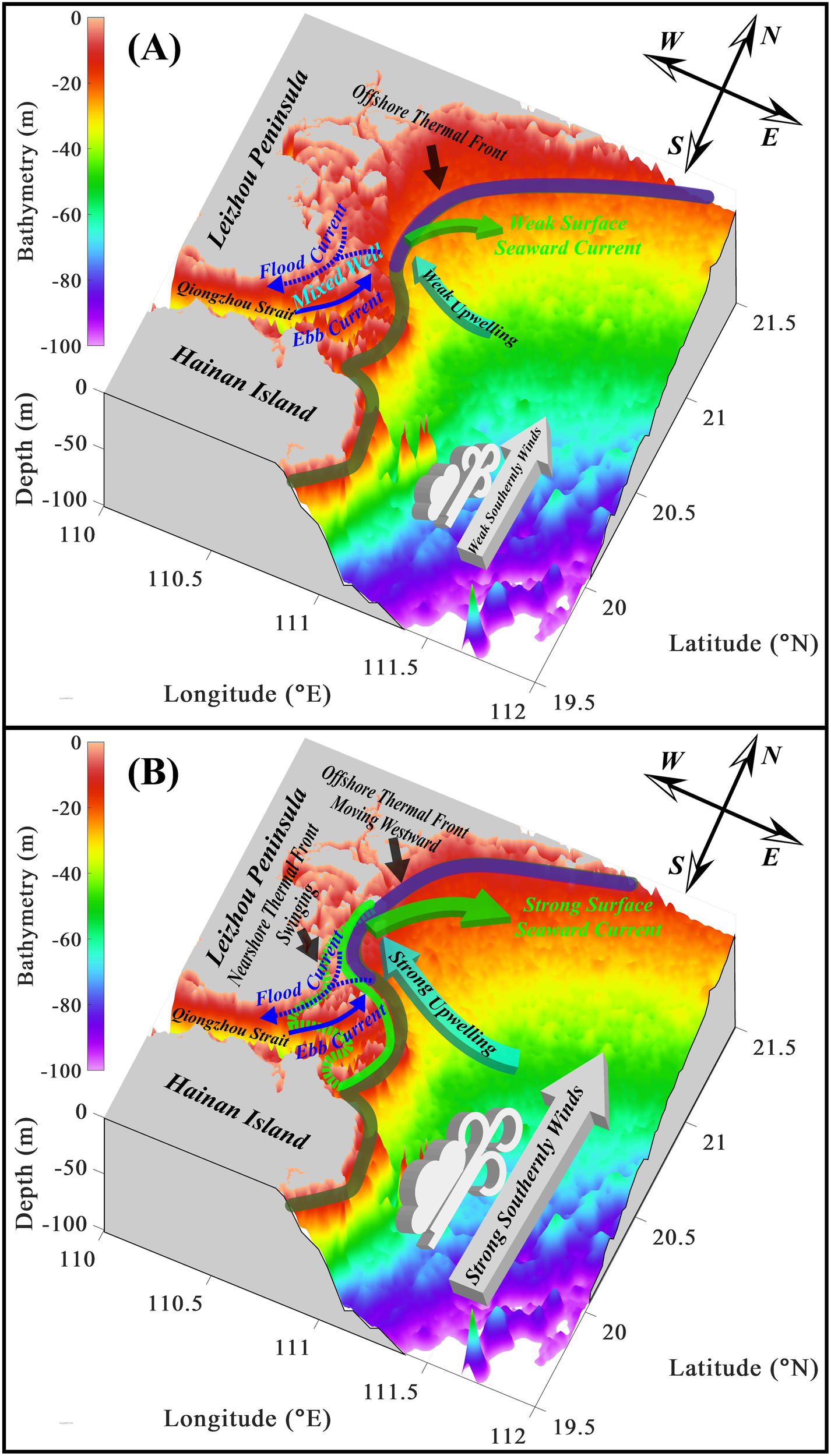
Figure 11. Conceptual diagram illustrating the underlying dynamics of how wind-driven coastal upwelling causes synoptic-to-intraseasonal variations in tidal temperature variability to the east of the Leizhou Peninsula and Qiongzhou Strait in the northern SCS in the summer. (A) Processes when southerly winds are weak. (B) Processes when southerly winds are strong.

Compared with previous studies (e.g., Wang et al., 2014; Hu and Wang, 2016; Lin and Gan, 2024), the important novel results of the current study are that wind-driven coastal upwelling can exert great impacts on synoptic-to-intraseasonal variations in tidal temperature variability. The current results highlight the importance of coastal upwelling/downwelling in modulating tidal temperature variability near ocean thermal fronts in the shelf seas. In addition, Li et al. (2024) observed significant near-inertial oscillations generated by wind bursting in the northern SCS, which could also potentially affect tidal temperature variability. In the future, more observations and high-resolution numerical simulations are still needed to understand the multi-scale variations in the magnitude of tidal variability in global shelf seas.

Data availability statement

The raw data supporting the conclusions of this article will be made available by the authors, without undue reservation.

Author contributions

JL: Data curation, Formal analysis, Methodology, Software, Validation, Visualization, Writing – original draft. FZ: Conceptualization, Formal analysis, Methodology, Supervision, Writing – review & editing. CL: Conceptualization, Formal analysis, Supervision, Writing – review & editing, Methodology. YG: Project administration, Writing – review & editing, Formal analysis. PL: Funding acquisition, Resources, Supervision, Writing – review & editing. GY: Writing – review & editing, Formal analysis.

Funding

The author(s) declare that financial support was received for the research and/or publication of this article. This work was jointly supported by the National Natural Science Foundation of China (Grant Nos. 42494881, 42206003) and the Research Startup Funding from Hainan Institute of Zhejiang University (Grant No. 0208-6602-A12202).

Acknowledgments

We appreciate the temperature data (MODIS-Aqua and MODIS-Terra) provided by NASA (https://oceancolor.gsfc.nasa.gov/l3/), the global ocean tidal atlases of Finite Element Solution 2014 (FES2014) provided by AVISO+ (https://www.aviso.altimetry.fr/en/data/products/auxiliary-products/global-tide-fes.html), the 41-layer Hybrid Coordinate Ocean Model and Navy Coupled Ocean Data Assimilation (HYCOM + NCODA) global 1/12° reanalysis data provided by Naval Research Laboratory (NRL, https://www.hycom.org/dataserver/gofs-3pt1/analysis), the Shuttle Radar Topography Mission (SRTM) 15Plus V2.1 provided by Scripps Institution of Oceanography (https://topex.ucsd.edu/WWW_html/srtm15_plus.html), and the ERA5 data provided by ECMWF (https://cds.climate.copernicus.eu/cdsapp#!/dataset/reanalysis-era5-single-levels?tab=form).

Conflict of interest

The authors declare that the research was conducted in the absence of any commercial or financial relationships that could be construed as a potential conflict of interest.

The reviewer XC declared a shared affiliation with the author FZ to the handling editor at the time of review.

Generative AI statement

The author(s) declare that no Generative AI was used in the creation of this manuscript.

Publisher’s note

All claims expressed in this article are solely those of the authors and do not necessarily represent those of their affiliated organizations, or those of the publisher, the editors and the reviewers. Any product that may be evaluated in this article, or claim that may be made by its manufacturer, is not guaranteed or endorsed by the publisher.

References

Bai P., Gu Y. Z., Li P. L., Wu K. J. (2016). Modelling the upwelling off the east Hainan Island coast in summer 2010. Chin. J. Oceanol. Limnol. 34, 1358–1373. doi: 10.1007/s00343-016-5147-5

Crossref Full Text | Google Scholar

Bai P., Yang J. L., Xie L. L., Zhang S. W., Ling Z. (2020). Effect of topography on the cold water region in the east entrance area of Qiongzhou Strait. Estuar. Coastal Shelf Sci. 242, 931–942. doi: 10.1016/j.ecss.2020.106820

Crossref Full Text | Google Scholar

Chen C. L., Li P. L., Shi M. C., Zuo J. C., Chen M. X., Sun H. P. (2009). Numerical study of the tides and residual currents in the Qiongzhou Strait. Chin. J. Oceanol. Limnol. 27, 931–942. doi: 10.1007/s00343-009-9193-0

Crossref Full Text | Google Scholar

Chen Y. C., Zhai F. G., Li P. L. (2020). Decadal variation of the kuroshio intrusion into the South China Sea during 1992–2016. J. Geophys. Res.: Oceans 125, e2019JC015699. doi: 10.1029/2019jc015699

Crossref Full Text | Google Scholar

Chen Y. C., Zhai F. G., Li P. L., Gu Y. Z., Wu K. J. (2022). Extreme 2020 summer SSTs in the northern South China Sea: implications for the Beibu Gulf coral bleaching. J. Climate 35, 4177–4190. doi: 10.1175/JCLI-D-21-0649.1

Crossref Full Text | Google Scholar

Cui L. B., Liu Z. Q., Chen Y., Cai Z. Y. (2024). Three-dimensional water exchanges in the shelf circulation system of the northern South China Sea under climatic modulation from ENSO. J. Geophys. Res.: Oceans 129, e2023JC020290. doi: 10.1029/2023JC020290

Crossref Full Text | Google Scholar

Gan J. P., Cheung A., Guo X. G., Li L. (2009). Intensified upwelling over a widened shelf in the northeastern South China Sea. J. Geophys. Res.: Oceans 114, C09019. doi: 10.1029/2007JC004660

Crossref Full Text | Google Scholar

Hu S., Li Y. N., Yu X. L., Gong W. P. (2024). Seasonal variations of coastal trapped waves (CTWs)’ propagation in the South China Sea. Estuar. Coastal Shelf Sci. 302, 108780. doi: 10.1016/j.ecss.2024.108780

Crossref Full Text | Google Scholar

Hu J. Y., Wang X. H. (2016). Progress on upwelling studies in the China seas. Rev. Geophysics 54, 653–673. doi: 10.1002/2015rg000505

Crossref Full Text | Google Scholar

Hu L. Y., Zhai F. G., Liu Z. Z., Gu Y. Z., Wu W. F., Li P. L., et al. (2024). Wind-driven nearshore overturning currents off the northeastern Shandong Peninsula in the Yellow Sea in winter. Front. Marine Sci. 11. doi: 10.3389/fmars.2024.1478811

Crossref Full Text | Google Scholar

Jing Z. Y., Qi Y. Q., Hua Z. L., Zhang H. (2009). Numerical study on the summer upwelling system in the northern continental shelf of the South China Sea. Continental Shelf Res. 29, 467–478. doi: 10.1016/j.csr.2008.11.008

Crossref Full Text | Google Scholar

Lao Q. B., Lu X., Chen F. J., Jin G. Z., Chen C. Q., Zhou X., et al. (2022). Effects of upwelling and runoff on water mass mixing and nutrient supply induced by typhoons: Insight from dual water isotopes tracing. Limnol. Oceanogr 68, 284–295. doi: 10.1002/lno.12266

Crossref Full Text | Google Scholar

Li Y. N., Curchitser E. N., Wang J., Peng S. Q. (2020). Tidal effects on the surface water cooling northeast of Hainan Island, South China Sea. J. Geophys. Res.: Oceans 125, e2019JC016016. doi: 10.1029/2019JC016016

Crossref Full Text | Google Scholar

Li J. Y., Li M., Xie L. L. (2024). Observations of near-inertial oscillations trapped at inclined front on continental shelf of the northwestern South China Sea. EGUsphere. doi: 10.5194/egusphere-2024-3909. (preprint).

Crossref Full Text | Google Scholar

Lin P. G., Cheng P., Gan J. P., Hu J. Y. (2016). Dynamics of wind-driven upwelling off the northeastern coast of Hainan Island. J. Geophys. Res.: Oceans 121, 1160–1173. doi: 10.1002/2015JC011000

Crossref Full Text | Google Scholar

Lin S. F., Gan J. P. (2024). Dynamics of tidal effects on coastal upwelling circulation over variable shelves in the northern South China Sea. J. Geophys. Res.: Oceans 129, e2024JC021193. doi: 10.1029/2024JC021193

Crossref Full Text | Google Scholar

Liu X. C., Gu Y. Z., Li P. L., Liu Z. Z., Wu K. J. (2020). A tidally dependent plume bulge at the Pearl River Estuary mouth. Estuar. Coastal Shelf Sci. 243, 106867. doi: 10.1016/j.ecss.2020.106867

Crossref Full Text | Google Scholar

Liu D. Y., Lv T., Lin L., Wei Q. S. (2022). Review of fronts and its ecological effects in the shelf sea of China. Adv. Marine Sci. 40, 725–741. doi: 10.12362/j.issn.1671-6647.20220719001. (In Chinese with English abstract).

Crossref Full Text | Google Scholar

Lü X. G., Qiao F. L., Wang G. S., Xia C. S., Yuan Y. L. (2008). Upwelling off the west coast of Hainan Island in summer: Its detection and mechanisms. Geophys. Res. Lett. 35, L02604. doi: 10.1029/2007GL032440

Crossref Full Text | Google Scholar

Lyard F. H., Allain D. J., Cancet M., Carrère L., Picot N. (2021). FES2014 global ocean tide atlas: design and performance. Ocean Sci. 17, 615–649. doi: 10.5194/os-17-615-2021

Crossref Full Text | Google Scholar

Mou L. Y., Niu Q. R., Xia M. (2022). The roles of wind and baroclinic processes in cross-isobath water exchange within the Bohai Sea. Estuar. Coastal Shelf Sci. 274, 107944. doi: 10.1016/j.ecss.2022.107944

Crossref Full Text | Google Scholar

Shi M. C., Chen C. S., Xu Q. C., Lin H. C., Liu G. M., Wang H., et al. (2002). The role of Qiongzhou strait in the seasonal variation of the South China Sea circulation. J. Phys. Oceanogr 32, 103–121. doi: 10.1175/1520-0485(2002)032<0103:TROQSI>2.0.CO;2

Crossref Full Text | Google Scholar

Shu Y. Q., Wang Q., Zu T. T. (2018). Progress on shelf and slope circulation in the northern South China Sea. Sci. China Earth Sci. 61, 560–571. doi: 10.1007/s11430-017-9152-y

Crossref Full Text | Google Scholar

Simpson J. H., Bowers D. (1981). Models of stratification and frontal movement in shelf seas. Deep Sea Res. Part A 28, 727–738. doi: 10.1016/0198-0149(81)90132-1

Crossref Full Text | Google Scholar

Song X., Lai Z., Ji R., Chen C., Zhang J., Huang L., et al. (2012). Summertime primary production in northwest South China Sea: Interaction of coastal eddy, upwelling and biological processes. Continental Shelf Res. 48, 110–121. doi: 10.1016/j.csr.2012.07.016

Crossref Full Text | Google Scholar

Tan K. Y., Xie L. L., Li M. M., Li M., Li J. Y. (2023). 3D structure and seasonal variation of temperature fronts in the shelf sea west of Guangdong. Haiyang Xuebao 45, 42–55. doi: 10.12284/hyxb2023053. (In Chinese with English abstract).

Crossref Full Text | Google Scholar

Tozer B., Sandwell D. T., Smith W. H. F., Olson C., Beale J. R., Wessel P. (2019). Global bathymetry and topography at 15 arc sec: SRTM15+. Earth Space Sci. 6, 1847–1864. doi: 10.1029/2019ea000658

Crossref Full Text | Google Scholar

Wang D. X., Liu Y., Qi Y. Q., Shi P. (2001). Seasonal variability of thermal fronts in the northern South China Sea from satellite data. Geophys. Res. Lett. 28, 3963–3966. doi: 10.1029/2001GL013306

Crossref Full Text | Google Scholar

Wang D. X., Shu Y. Q., Xue H. J., Hu J. Y., Chen J., Zhuang W., et al. (2014). Relative contributions of local wind and topography to the coastal upwelling intensity in the northern South China Sea. J. Geophys. Res.: Oceans 119, 2550–2567. doi: 10.1002/2013jc009172

Crossref Full Text | Google Scholar

Wang D. R., Yang Y., Wang J., Bai X. Z. (2015). A modeling study of the effects of river runoff, tides, and surface wind-wave mixing on the Eastern and Western Hainan upwelling systems of the South China Sea, China. Ocean Dynamics 65, 1143–1164. doi: 10.1007/s10236-015-0857-3

Crossref Full Text | Google Scholar

Wu W. F., Li P. L., Zhai F. G., Gu Y. Z., Liu Z. Z. (2020). Evaluation of different wind resources in simulating wave height for the Bohai, Yellow, and East China Seas (BYES) with SWAN model. Continental Shelf Res. 207, 104217. doi: 10.1016/j.csr.2020.104217

Crossref Full Text | Google Scholar

Wu W. F., Song C. Y., Chen Y. C., Zhai F. G., Liu Z. Z., Liu C., et al. (2025). High-frequency dynamics of bottom dissolved oxygen in temperate shelf seas: the joint role of tidal mixing and sediment oxygen demand. Limnol. Oceanogr 70, 1–14. doi: 10.1002/lno.12733

Crossref Full Text | Google Scholar

Wu W. F., Zhai F. G., Liu C., Gu Y. Z., Li P. L. (2023a). Three-dimensional structure of summer circulation in the Bohai Sea and its intraseasonal variability. Ocean Dynamics 73, 679–698. doi: 10.1007/s10236-023-01576-6

Crossref Full Text | Google Scholar

Wu W. F., Zhai F. G., Liu Z. Z., Liu C., Gu Y. Z., Li P. L. (2023b). The spatial and seasonal variability of nutrient status in the seaward rivers of China shaped by the human activities. Ecol. Indic. 157, 111223. doi: 10.1016/j.ecolind.2023.111223

Crossref Full Text | Google Scholar

Xie L. L., Chen L., Zheng Q., Wang G., Yu J., Xiong X., et al. (2024). Mechanisms of reappeared period shifts of internal solitary waves based on mooring array observations in the northern South China Sea. J. Geophys. Res.: Oceans 129, e2023JC020389. doi: 10.1029/2023JC020389

Crossref Full Text | Google Scholar

Xie L. L., Enric P.-S., Zheng Q., Zhang S. W., Zong X. L., Yi X. F., et al. (2017). Diagnosis of 3D vertical circulation in the upwelling and frontal zones east of Hainan Island, China. J. Phys. Oceanogr 47, 755–774. doi: 10.1175/JPO-D-16-0192.1

Crossref Full Text | Google Scholar

Xie L. L., Zhang S. W., Chen, Zhao H. (2012). Overview of studies on Qiongdong upwelling. J. Trop. Oceanogr 31, 35–41. doi: 10.3969/j.issn.1009-5470.2012.04.005

Crossref Full Text | Google Scholar

Xu F. H., Oey L. Y. (2015). Seasonal SSH variability of the northern South China Sea. J. Phys. Oceanogr 45, 1595–1609. doi: 10.1175/JPO-D-14-0193.1

Crossref Full Text | Google Scholar

Yan C. Y., Gu Y. Z., Li P. L., Zhai F. G., Liu C., He S. Y., et al. (2024). Bi-layered spring-neap variability of water masses in estuaries and the impact of human activities. Water Res. 266, 122413. doi: 10.1016/j.watres.2024.122413

PubMed Abstract | Crossref Full Text | Google Scholar

Yan D., Song D. H., Bao X. W. (2020). Spring-neap tidal variation and mechanism analysis of the maximum turbidity in the Pearl River Estuary during flood season. J. Trop. Oceanogr 39, 20–35. doi: 10.11978/2019035

Crossref Full Text | Google Scholar

Yang F., Ji X. M., Zhang W., Zou H. Z., Jiang W. Z., Xu Y. W. (2022). Characteristics and driving mechanisms of salinity stratification during the wet season in the Pearl River Estuary, China. J. Marine Sci. Eng. 10, 1927. doi: 10.3390/jmse10121927

Crossref Full Text | Google Scholar

Yu B., Liu Z. Z., Zhai F. G., Gu Y. Z., Wu W. F. (2022). Study on the diurnal variation in the bottom layer dissolved oxygen in Yutai Marine Ranch off Weihai in the summer of 2020. Marine Environ. Sci. 41, 563–571. doi: 10.12111/j.mes.2021-x-0070

Crossref Full Text | Google Scholar

Yuan Y. C., Liao G. H., Yang C. H. (2009). A diagnostic calculation of the circulation in the upper and middle layers of the Luzon Strait and the northern South China Sea during March 1992. Dynamics Atmos. Oceans 47, 86–113. doi: 10.1016/j.dynatmoce.2008.10.005

Crossref Full Text | Google Scholar

Zhai F. G., Li P. L., Gu Y. Z., Li X., Chen D., Li L., et al. (2020). Review of the research and application of the submarine cable online observation system. Marine Sci. 44, 14–28. doi: 10.11759/hykx20200331003

Crossref Full Text | Google Scholar

Zhai F. G., Liu Z. Z., Li P. L., Gu Y. Z., Sun L. Y., Hu L. Y., et al. (2021). Physical controls of summer variations in bottom layer oxygen concentrations in the coastal hypoxic region off the Northeastern Shandong Peninsula in the Yellow Sea. J. Geophys. Res.: Oceans 126, e2021JC017299. doi: 10.1029/2021jc017299

Crossref Full Text | Google Scholar

Zhang Y. L., Ateljevich E., Yu H. C., Wu C. H., Yu J. C. (2015). A new vertical coordinate system for a 3D unstructured-grid model. Ocean Modelling 85, 16–31. doi: 10.1016/j.ocemod.2014.10.003

Crossref Full Text | Google Scholar

Zhang Y. L., Baptista A. M. (2008). SELFE: A semi-implicit Eulerian-Lagrangian finite-element model for cross-scale ocean circulation. Ocean Modelling 21, 71–96. doi: 10.1016/j.ocemod.2007.11.005

Crossref Full Text | Google Scholar

Zhang Y. L., Ye F., Stanev E. V., Grashorn S. (2016). Seamless cross-scale modeling with SCHISM. Ocean Modelling 102, 64–81. doi: 10.1016/j.ocemod.2016.05.002

Crossref Full Text | Google Scholar

Zhang Y., Zeng L. L., Wang Q., Geng B. X., Liu C. J., Shi R., et al. (2021). Seasonal variation in the three-dimensional structures of coastal thermal front off western Guangdong. Acta Oceanologica Sin. 40, 88–99. doi: 10.1007/s13131-021-1739-9

Crossref Full Text | Google Scholar

Zhi H. H., Wu H., Wu J. X., Zhang W. X., Wang Y. H. (2022). River plume rooted on the sea-floor: seasonal and spring-neap variability of the Pearl River plume front. Front. Marine Sci. 9. doi: 10.3389/fmars.2022.791948

Crossref Full Text | Google Scholar

Zu T. T., Gan J. P., Svetlana Y. E. (2007). Numerical study of the tide and tidal dynamics in the South China Sea. Deep Sea Res. Part I: Oceanographic Res. Pap. 55, 137–154. doi: 10.1016/j.dsr.2007.10.007

Crossref Full Text | Google Scholar