Intelligent forecasting model for aquatic production based on artificial neural network

Accurate forecasting of aquatic production is critical for sustainable fisheries management. In this study, four neural network models, namely Back Propagation (BP) neural network, BP neural networks optimized by Genetic Algorithms (GA-BP), Long Short-Term Memory neural networks (LSTM), and Radial Basis Function neural networks (RBF), are developed and compared to predict aquatic production in Zhanjiang City, China. First, key influencing factors are identified through Grey Relational Analysis (GRA), including GDP per capita, sunshine duration, and Engel coefficient. The models are trained and tested using historical production data, with performance evaluated by R² and MAE metrics. Results show that the RBF neural network achieves the highest prediction accuracy (R²=0.96, MAE=27725), significantly outperforming BP (R²=0.73), GA-BP (R²=0.93), and LSTM (R²=0.94). Sensitivity analysis is then conducted to rank the influencing factors by importance. GDP per capita is found to be the most critical factor, followed by climate-related variables (sunshine duration, temperature) and socioeconomic indicators (Engel coefficient, consumer price index). The robustness of the RBF model suggests that it can be effectively applied for regional aquatic production forecasting, supporting policymakers in resource allocation and risk mitigation. Furthermore, the factor prioritization enables aquaculture practitioners to optimize farming strategies, such as adjusting production scales based on economic and environmental trends. This study not only provides a reliable modeling framework but also highlights the key drivers affecting aquatic production, including economic, climatic, and demographic factors.

1 Introduction

Aquaculture is recognized as a critical component of global food security and economic development, playing an indispensable role in meeting nutritional needs and supporting livelihoods worldwide. However, the industry currently faces unprecedented challenges in production forecasting due to increasing climate variability, resource constraints, and market fluctuations. These challenges highlight the urgent need for more accurate prediction models to support sustainable sector development.

Three main approaches are currently employed in aquatic production forecasting, each presenting distinct advantages and limitations. Statistical methods (Tan and Deng, 1995; Cho, 2006; Ghani and Ahmad, 2010; Anthony Koslow and Davison, 2016; Benavides et al., 2022; Kalhoro et al., 2024), including time series analysis and regression models, are widely applied in fisheries research. Autoregressive Integrated Moving Average (ARIMA) models are demonstrated to be effective for specific applications, as shown by Siddique et al. (2024) in tilapia production forecasting. However, these methods are found to struggle with complex nonlinear relationships that characterize modern aquaculture systems (Benavides et al., 2022; Kalhoro et al., 2024). Ecological modeling approaches (Tsitsika et al., 2010; Naorem et al., 2013; Raman et al., 2017; Panwar et al., 2018; Siddique et al., 2024) are developed to address these limitations by incorporating environmental parameters. The ecological modeling approach considers the impact of the ecological environment on aquatic production, including factors such as water temperature, salinity, dissolved oxygen, and others. By integrating principles of biology and ecology, the ecological modeling approach establishes ecological models for prediction. The ecological modeling method can comprehensively reflect the impact of environmental factors on yield, but the model construction is complex and requires a large amount of data (Naorem et al., 2013; Raman et al., 2017; Deng, 1990).

Machine learning techniques (Rahman et al., 2021; Zhao et al., 2021; Miguéis et al., 2022; Stephen et al., 2022; Law et al., 2019) are increasingly adopted to overcome these challenges. Miguéis et al. (2022); Law et al., 2019 proposed a daily fresh fish demand forecasting model to promote a more sustainable supply chain and prevent food waste. They used a representative store of a large European retail company as an example to estimate the demand for fresh fish by long short-term memory networks (LSTM), feedforward neural networks, support vector regression, random forests, and Holt Winters statistical models. The research results showed that compared with baseline and statistical models, machine learning models provided accurate predictions. To obtain control variables suitable for predicting fish catch, based on the “Annual Fisheries Statistics” data released by the Malaysian Ministry of Fisheries, Ghani and Ahmad (2010) used stepwise multiple regression method with Minitab 15 and SPSS 17.0 for analysis. Their research showed that the number of fishermen and the number of fishing gear licenses are factors affecting the catch of marine fish. Jasmin et al. (2022) used the average dissolved oxygen and biological floc count in shrimp farming systems as target parameters, and considered 17 farming and meteorological parameters. Three different feature selection techniques are used to create 12 different data subsets for model development. The model development utilized three popular machine learning algorithms, namely Random Forest, AdaBoost, and Deep Neural Networks. A total of 36 different models are obtained and their accuracy is evaluated by 7 model validation tests. Cross-disciplinary researchers are introduced by Quetglas et al. (2011) to how artificial neural networks are applied in ecology, while ecologists unfamiliar with artificial neural networks are assisted in understanding the diverse practical applications of these tools in aquatic ecology. Machine learning methods refer to training models on a large amount of historical data to obtain forecasting models, mainly including support vector machines, random forests, and neural networks. Aquatic production is influenced by a series of factors, and aquatic production prediction is a typical nonlinear problem. Neural networks have strong nonlinear mapping and self-learning abilities. Current research shows that neural network algorithms have great potential in aquatic production prediction, and establishing accurate aquatic production forecasting models by neural network algorithms is theoretically feasible.

Zhanjiang City is recognized as a vital aquaculture center in southern China, where an annual industrial output value exceeding 70 billion yuan is generated by the aquatic product industry chain, while employment opportunities for over 1 million people are directly and indirectly created (Zhanjiang Statistical Yearbook, 2023). Despite its economic significance, Zhanjiang lacks a tailored forecasting framework that accounts for its unique confluence of subtropical climate, extensive coastal aquaculture, and evolving socioeconomic factors-including rising per capita GDP, changing consumption patterns, and fluctuating labor demographics. Existing regional studies either rely on oversimplified statistical models or overlook Zhanjiang’s specific challenges, leaving policymakers and industry stakeholders without actionable predictive tools. To resolve the aforementioned dilemmas, a targeted multi-phase forecasting methodology for aquatic production in Zhanjiang is developed in this research. Grey Relational Analysis (GRA) is utilized to systematically identify the most influential variables affecting local aquatic production, with integration of environmental (temperature, sunshine duration), socioeconomic (GDP per capita, Engel coefficient), and operational (aquaculture area, fishery population) factors. A comprehensive dataset is compiled from the Guangdong Rural Yearbook and Zhanjiang Statistical Yearbook, ensuring temporal depth and regional specificity. Four neural network architectures, namely Back Propagation (BP) neural network, BP neural networks optimized by Genetic Algorithms (GA-BP), LSTM, and Radial Basis Function neural networks (RBF), are deployed to develop predictive models, with rigorous performance evaluation using R² and MAE metrics. Neural network parameter sensitivity analysis is applied to rank the importance of identified factors, providing clear guidance for targeted intervention strategies.

The novelty of this approach lies in three interconnected advancements: (1) its explicit focus on Zhanjiang’s unique regional dynamics, (2) the integration of 12 multi-dimensional influencing factors rarely combined in existing models, and (3) a comparative framework that identifies the optimal neural network architecture for coastal aquaculture contexts. By addressing the limitations of statistical oversimplification, ecological data dependency, and generic machine learning approaches, both a methodologically robust forecasting tool and actionable insights for Zhanjiang’s aquaculture sector are delivered in this study-ultimately supporting sustainable growth, market stability, and informed policy formulation.

2 Data and methods

2.1 Data selection

Based on the current research progress (Jaureguizar et al., 2024), the restrictive factors affecting the output of aquatic products in Zhanjiang City from 1992 to 2022 have been obtained from the Guangdong Rural Yearbook and Zhanjiang Statistical Yearbook. These factors include the total aquaculture area, the number of motorized fishing vessels, the fishery population, the annual average temperature, and the sunshine durations. Moreover, considering that the residents of Zhanjiang City are an important consumer group of aquatic products, this paper also takes into account the influences of Zhanjiang’s Engel coefficient, consumer price index, household registered population, and per capita GDP on the output of aquatic products. The first nine rows of Table 1 show the above nine factors, and the tenth row indicates the output of aquatic products in Zhanjiang City. The following content will continue to study the impacts of these nine influencing factors on the output of aquatic products in Zhanjiang City.

Table 1

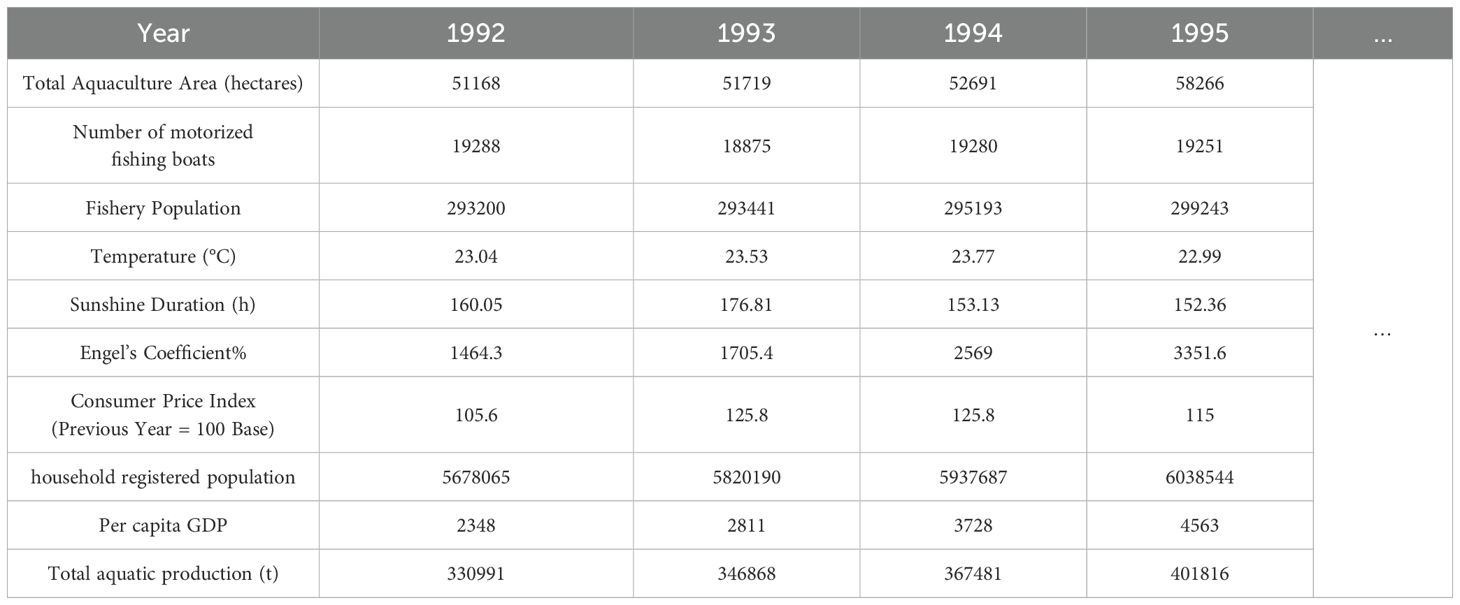
Table 1. Partial data on factors affecting aquatic production in Zhanjiang City.

2.2 Grey relational analysis

Grey relational analysis(GRA) is an important method within the theory of grey systems, originally proposed by the renowned scholar Professor Deng Julong. The theoretical foundation of this analysis method lies in determining the degree of correlation between different factors by comparing the geometric similarity of their change curves. In this paper, the grey correlation analysis is used to quantitatively determine the degree of correlation between aquaculture area, number of motorized fishing boats, fishery population, average annual temperature, sunshine duration, Engel coefficient, consumer price index, total number of registered residence registered persons, per capita GDP and aquatic production. This paper uses the nine influencing factors mentioned above as comparative sequences and aquatic production as the reference sequence for GRA. The specific steps are as follows:

2.2.1 Data normalization

Construct matrix $A_{10\times 31}$ using the complete dataset in Table 1, with the first 9 rows as the comparison sequence and the 10th row as the reference sequence. Due to the different dimensions of the data in each row of matrix $A_{10\times 31}$, it is necessary to use the mean normalization method to standardize and obtain the standardized matrix $B_{10\times 31}$. The element $b_{ij}$ in $B_{10\times 31}$ is calculated by Equation 1.

$\begin{array}{ll}{b}_{ij}=\frac{a_{ij}}{\overline{a_{ij}}}& (1)\end{array}$

Where, $a_{ij}$ represents the elements in matrix $A_{10\times 31}$, and $\overline{a_{ij}}$ is the mean value of the elements in each row of $A_{10\times 31}$, i=1,2,…10, j=1,2,…31. When i=10, b_10,j represents the normalized values of the reference sequence.

2.2.2 Calculate the grey relational coefficients between the reference sequence and the reference sequence

Construct the correlation coefficient matrix C, and calculate the elements in C using Equation 2.

$\begin{array}{ll}{c}_{ij}=\frac{min\left|b_{ij}-b_{10,j}\right|+\rho max\left|b_{ij}-b_{10,j}\right|}{b_{ij}+\rho max\left|b_{ij}-b_{10,j}\right|},i=1,2,\mathrm{\dots 9}& (2)\end{array}$

Where the resolution coefficient $\text{ρ}ϵ(0,1]$, and the resolution coefficient is set to 0.5 in this paper. The results of the first four columns of matrix C are shown in Table 2.

Table 2

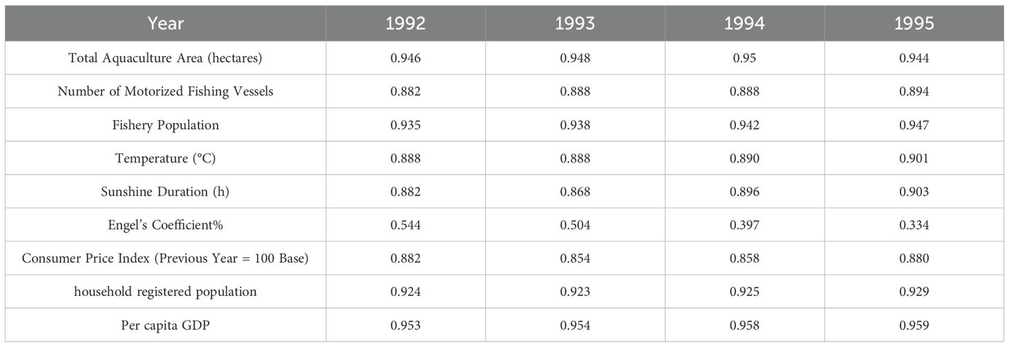
Table 2. The first four columns of data in the correlation coefficient matrix.

2.2.3 Calculate the value of GRA

The element c_ij in the correlation matrix C represents the degree of correlation between the i-th influencing factor and the production in the j-th year. Using $r_i=\frac{1}{31}{\displaystyle {\sum }_{j=1}^{31}{c}_{ij}}$, the correlation degree between various influencing factors and aquatic production can be obtained. The results are shown in Table 3.

Table 3

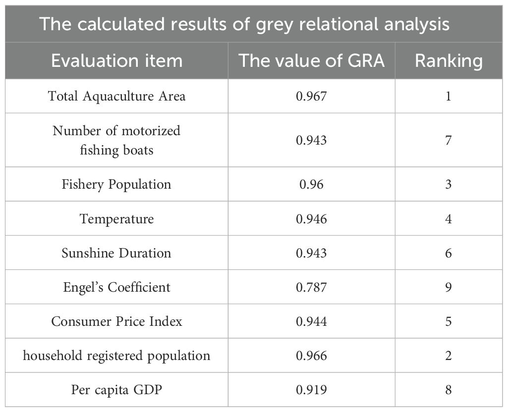
Table 3. Correlation and ranking of various influencing factors with aquatic production.

The GRA value ranges between 0 and 1. The closer its value is to 1, the stronger the correlation with the reference sequence (aquatic production). According to Table 3, the correlation values between the top eight influencing factors and aquatic production are all above 0.9, and the correlation value between the last ranked influencing factor, the Engel coefficient, and aquatic production is also as high as 0.787, indicating that the nine influencing factors selected in this paper have a strong correlation with aquatic production. So, this paper selects the nine influencing factors mentioned above as input parameters for the neural network.

3 Aquaculture production forecasting model based on BP neural network

3.1 BP neural network

The establishment of a BP neural network model mainly involves three steps: initialization of network parameters, forward propagation of information, and backward propagation of errors. The basic structure of a BP neural network includes an input layer, hidden layers (which can be one or multiple), and an output layer, with each layer potentially containing multiple neurons. A schematic diagram of a BP neural network is shown in Figure 1.

Figure 1

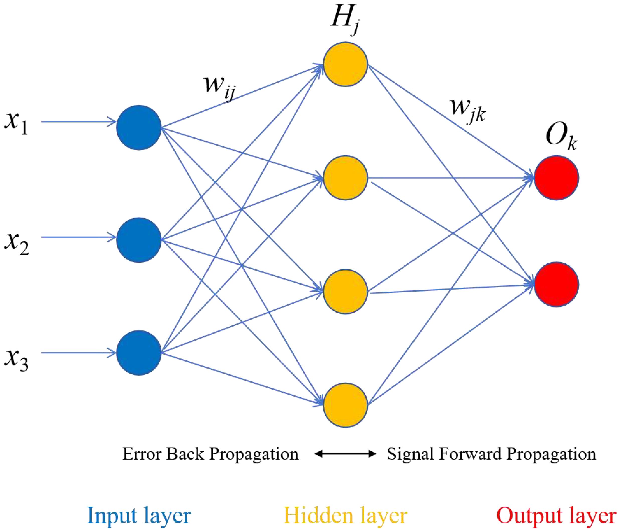
Figure 1. BP neural network structure.

The information received by the input layer is the learning sample after network parameter initialization, which is then passed to each neuron in the hidden layer by Equation 3.

$\begin{array}{ll}{H}_j=f({\displaystyle {\sum }_{i=1}^n{\omega }_{ij}{x}_i+b_j})& (3)\end{array}$

The output value of the output layer is calculated using the Equation 4.

$\begin{array}{ll}{O}_k={\displaystyle {\sum }_{j=1}^l{H}_j{\omega }_{jk}+b_k}& (4)\end{array}$

The error between the network output value and the actual value y_k is the function $e_{\text{k}}$, and the sum of $e_{\text{k}}$ is the objective function E. See Equation 5 for details.

$\begin{array}{ll}\text{E}={\displaystyle {\sum }_{\text{k}=1}^{\text{m}}{e}_{\text{k}}}={\displaystyle {\sum }_{\text{k}=1}^{\text{m}}(y_k-O_{k })}& (5)\end{array}$

If E ≤ ϵ is satisfied, the algorithm ends. Otherwise, error back-propagation calculation is performed to update weights and biases. The update formula is shown below. See Equations 5, 6 for details.

$\begin{array}{ll}{\omega }_{ij}(t+1)={\omega }_{ij}(t)+\eta \frac{\partial E(t)}{\partial {\omega }_{ij}(t)}& (6)\end{array}$

$\begin{array}{ll}{b}_j(t+1)=b_j(t)+\eta \frac{\partial E(t)}{\partial b_j(t)}& (7)\end{array}$

In the above five equations, ${\omega }_{ij}(t+1)$ and $b_j(t+1)$ respectively represent the connection weight and bias value between the ith neuron in the input layer and the jth neuron in the hidden layer at the (t+1)th iteration. n, l, and m are the number of nodes in the input layer, hidden layer, and output layer, respectively. $\omega$ and b are the parameters that need to be learned during training, η is the learning rate, and f is the activation function. Non-linear activation functions enable neural networks to better learn complex data patterns, thereby enhancing their expressive power and learning capabilities. Common activation functions include the sigmoid function (also known as the S-shaped function) and the hyperbolic tangent activation function (also known as the bipolar S-shaped function). The sigmoid function is commonly used in binary classification problems, which can map real numbers to the (0,1) interval. The equation is as follows:

$\begin{array}{ll}logsig(x)=\frac{1}{1+e^{-x}}& (8)\end{array}$

The hyperbolic tangent activation function maps real numbers to the interval (-1,1). The formula for this function is as follows. See Equation 9 for details:

$\begin{array}{ll}tansig(x)=\frac{2}{1+e^{-2x}}-1& (9)\end{array}$

3.2 Modeling with BP neural networks

3.2.1 Data initialization

Based on a total of 31 sets of historical data from 1992–2022 in Zhanjiang City, a neural network training and testing dataset is constructed. Eliminate the influence of element dimension on input neurons through Equation 10.

$\begin{array}{ll}{x}_{ij}=\frac{a_{ij}—min{a}_{ij}}{max{a}_{ij}—min{a}_{ij}}& (10)\end{array}$

3.2.2 Model parameter initialization

Before model training, the weights w_ij and w_jk, as well as the biases b_j and b_k, of the neural network are randomly initialized. The maximum number of iterations for the network is set to τ=1000, the error threshold is set to ϵ=1×10^-6, and the learning rate is set to η=0.01. The number of neurons in the hidden layer is set to 6, with a total of 1 hidden layer.

3.2.3 Training of BP neural network

In model training, the logsign function (Equation 8) is used as the activation function to assign input information to the (0,1) interval, and the result is passed to the hidden layer neurons. Then, the pureline activation function shown in Equation 11 is used to pass the information to the output layer, and the output result can be represented by Equation 4.

$\begin{array}{ll}f(t)=t& (11)\end{array}$

Equation 12 is selected to calculate the error E between the output value and the true value.

$\begin{array}{ll}\text{E}={\displaystyle {\sum }_{\text{k}}{e}_{\text{k}}}=\sqrt{{\displaystyle {\sum }_{\text{k}}{(y_k-O_{k })}^2}}& (12)\end{array}$

Then, compare the error E with the error threshold ϵ. When the error E ≤ ϵ or the iteration reaches 1000 times, output the corresponding weights and biases. Otherwise, the network performs backward adjustment based on the error, using gradient descent to achieve error correction.

3.2.4 Neural network model testing

The model’s accuracy is validated using a test dataset. The test dataset is input into the model trained in step (3), and the model’s performance is evaluated based on the R² and MAE metrics. R² assesses the closeness of the model’s predicted values to the actual values, where an R² closer to 1 indicates a better fit. MAE measures the average magnitude of prediction errors, and without considering the direction of the errors, a smaller value indicates higher precision. The flowchart of the BP neural network is shown in Figure 2.

Figure 2

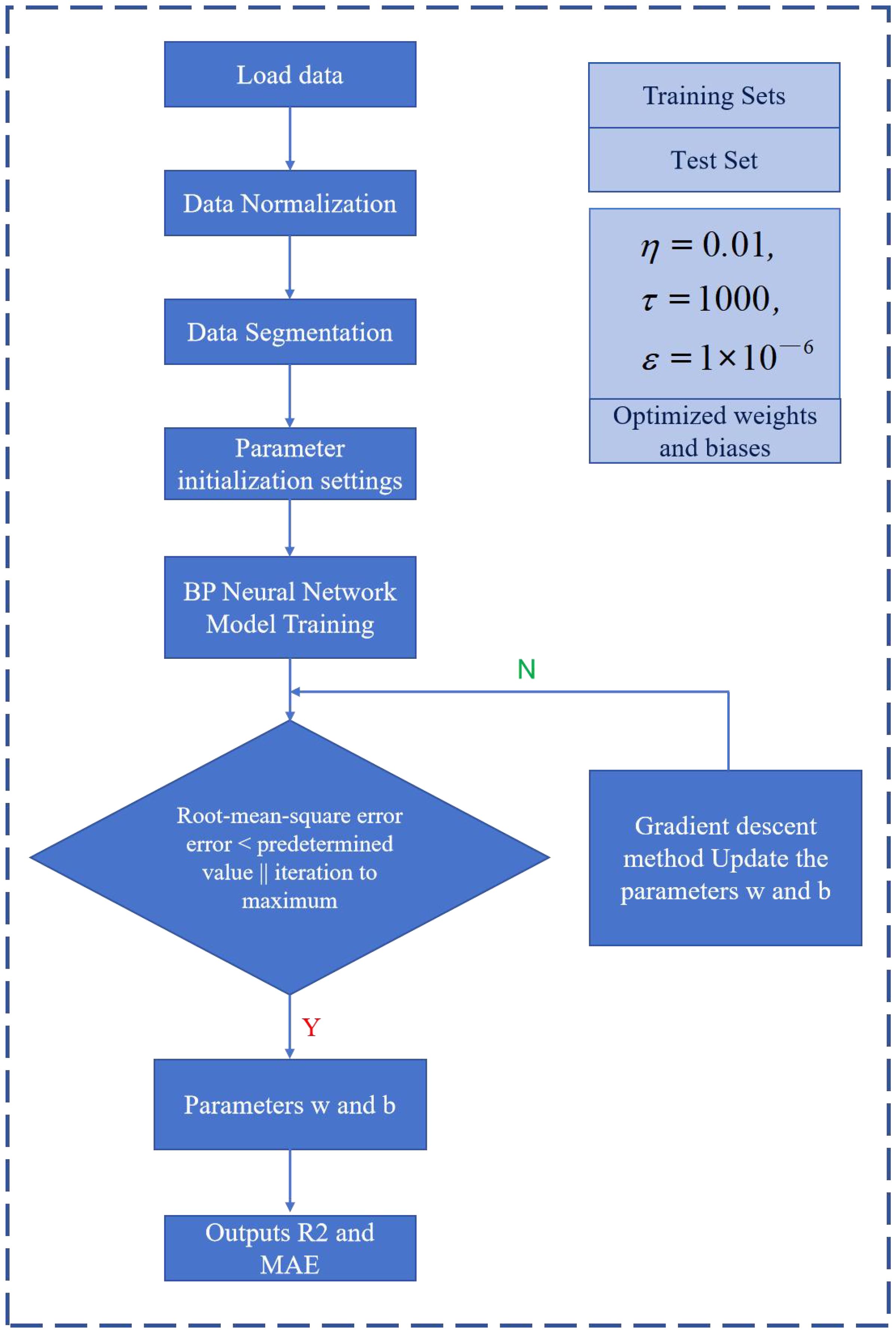
Figure 2. Flowchart of BP neural network.

3.3 Aquaculture production forecasting model

Figures 3 and 4 show the comparison results between the true values and the forecasting values of the training and testing sets, respectively. The R² and MAE of the training set are 0.92 and 73700, respectively, while the R² and MAE of the testing set are 0.73 and 92995, respectively. The weights and biases of the aquatic production forecasting model based on BP neural network in Zhanjiang City are shown in Tables 4 and 5. Considering the statistical data of the training set comprehensively, it can be concluded that the aquatic production forecasting model based on BP neural network established in this paper has good performance. However, the R² value of the testing set is low, and the forecasting values of the test set fluctuate greatly. This is because the initial weights and biases of the BP neural network are randomly specified, which makes the established forecasting model prone to falling into local minima and causing a decrease in accuracy. To solve this problem, this paper combines GA with BP neural network, uses GA to optimize the initial weights and biases of BP neural network, and establishes a high-precision and robust Zhanjiang aquatic production forecasting model based on GA-BP neural network.

Figure 3

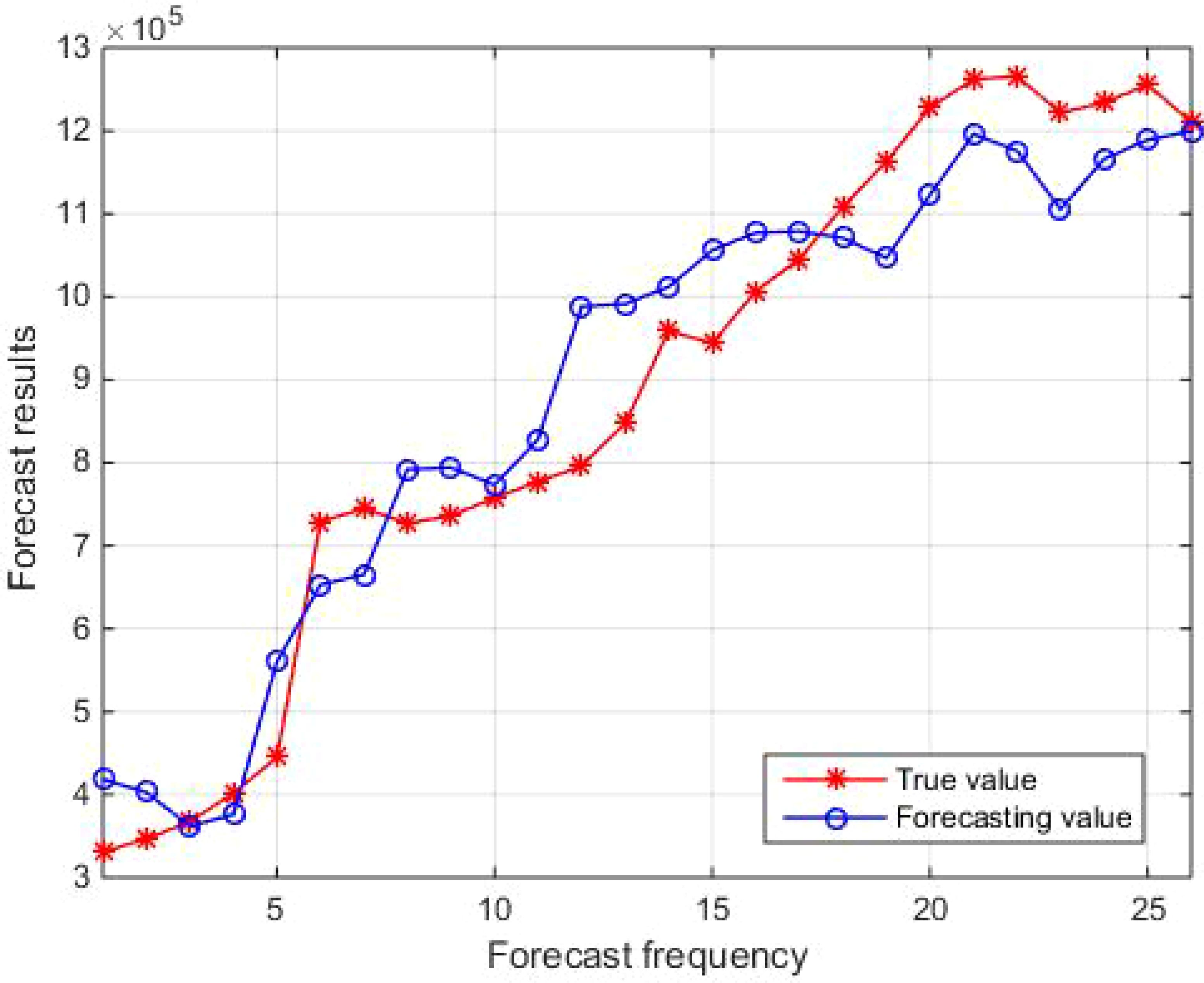
Figure 3. Comparison of true and forecasting values in the training set.

Figure 4

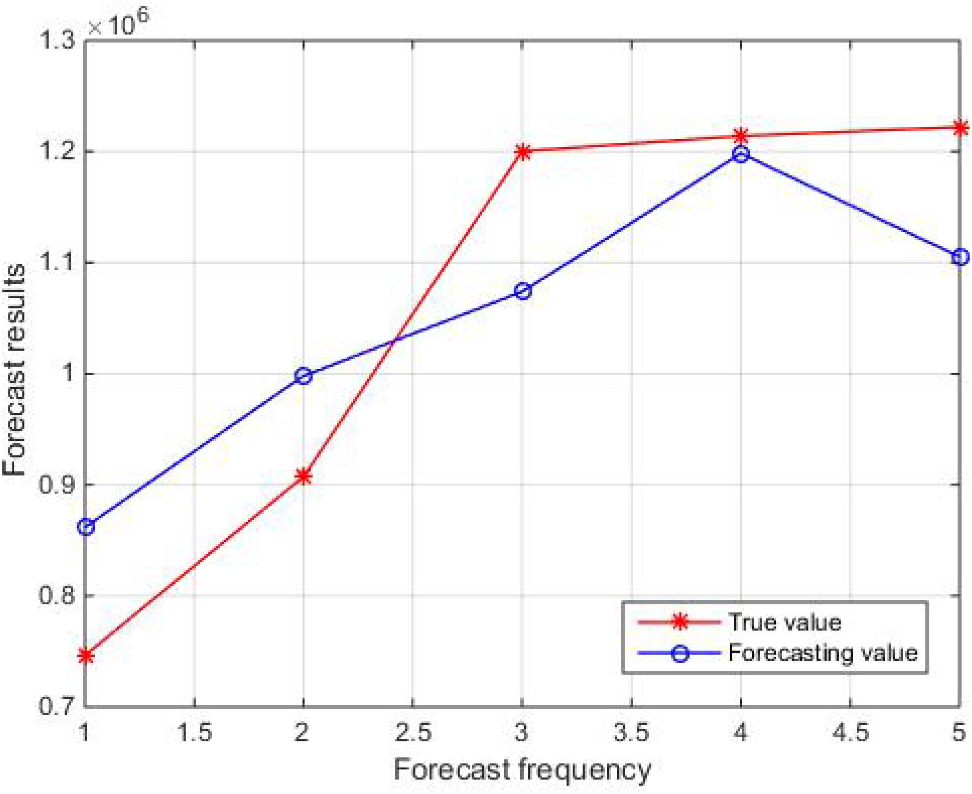
Figure 4. Comparison of true and forecasting values in the testing set.

Table 4

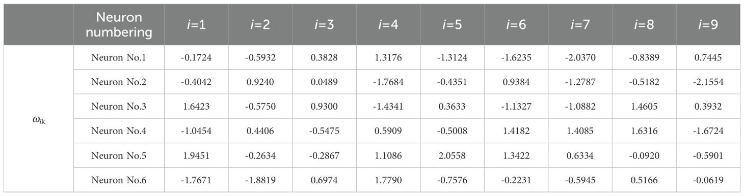
Table 4. The results of the weights (ω_ik) from the input layer to the hidden layer.

Table 5

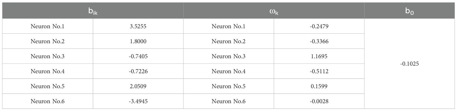
Table 5. b_ik, ω_k, and b₀ parameter table.

4 Aquaculture production forecasting model based on GA-BP neural network

4.1 Basic principles of GA

Genetic algorithms represent the data in the solution space as genotype string structure data in the genetic space before searching, and by choosing a reasonable coding mechanism, utilize a certain coding form of the solution to evolve in order to improve the algorithm and efficiency, and then realize the diversity of the solution by crossover, mutation and other operations. Crossover operation is the most important genetic operation in genetic algorithm, which randomly matches individuals in a population into pairs and exchanges part of chromosomes between them with a certain probability (known as Crossover Rate, P_c); Mutation operation is that the value of a string in the genotypic string structure data is changed with a certain probability (known as Mutation Rate, P_m). Genetic algorithms basically do not use external information during the evolution process, but are based on fitness functions, designing fitness functions from the objective function and ultimately retaining better individuals.

4.2 GA-BP neural network operation steps

4.2.1 Coding

To obtain reasonable initial weights and thresholds for the BP neural network, a real number encoding method IS used for optimization. The encoding length S=R*S₁+S₁*S₂+S₁+S₂, where R, S₁, and S₂ are the number of input layer nodes, hidden layer nodes, and output layer nodes of the BP neural network, respectively. In the aquaculture production forecasting problem in Zhanjiang City, R=9, S₁ = 6, S₂ = 1, and the encoding length S=67.

4.2.2 Fitness function

The fitness function is used to measure individual adaptability, that is, to measure the error between predicted values and actual values. Evaluate the quality of genes after selection, crossover, and mutation operations, train the data using a BP neural network, and use the reciprocal of the root mean square error between the predicted value O_i and the actual value y_i as the fitness function. The specific equation is shown below. See Equation 13 for details.

$\begin{array}{ll}fit=\frac{1}{\sqrt{\frac{1}{n}{{\displaystyle \sum }}_{i=1}^n{(y_i-o_i)}^2}}& (13)\end{array}$

4.2.3 Initialize the population

Set the initial population size to P=10, and then randomly generate an initial population of P individuals, W=(W₁, W₂,…, W_p)^T.

4.2.4 Choose

In genetic algorithms, selection operations are used to determine which individuals can be selected as the parent individuals for the next generation. Choose normalGeomSelect for selection operation, which is a type of normalized geometric selection. By normalizing the fitness values of individuals and selecting parent individuals based on the normalized fitness values. Specifically, the following equation is used to calculate the probability of an individual in the selection process. See Equation 14 for details.

$\begin{array}{ll}\text{Prob}(i)=(1-p)p^i& (14)\end{array}$

4.2.5 Crossover operation

Using the real number crossover method as the crossover operator, the calculation equation for the crossover operation between the kth and ith chromosomes at position l is described as follows. See Equation 15 for details.

$\begin{array}{ll}\{\begin{array}{c}{a}_{kj}=a_{kj}(1-b)+a_{ij}b\\ a_{ij}=a_{ij}(1-b)+a_{kj}b\end{array}& (15)\end{array}$

Where b is a random number of [0, 1].

4.2.6 Mutation

To maintain population diversity and prevent the population from falling into a local optimum, genetic mutation is necessary. The calculation equation for single-point mutation on the jth gene of the ith individual is as follows. See Equation 16 for details.

$\begin{array}{ll}{a}_{ij}=\{\begin{array}{cc}{a}_{ij}+(a_{ij}-a_{max})rF& r>0.5\\ a_{ij}+(a_{min}-a_{ij})rF& r\le 0.5\end{array}& (16)\end{array}$

where a_max and a_min are the upper and lower bounds of genes a_ij, respectively, r is a random number of [0,1], $F={(1-\text{g}/{\text{G}}_{\text{max}})}^2$, g is the current iteration count, G_max is the maximum evolution count, G_max=30.

The optimal weights and thresholds obtained by the genetic algorithm are substituted as the initial weights and biases into the BP neural network, and then the training data set is used to build a model for the neural network. The flowchart of the GA-BP neural network is shown in Figure 5 below.

Figure 5

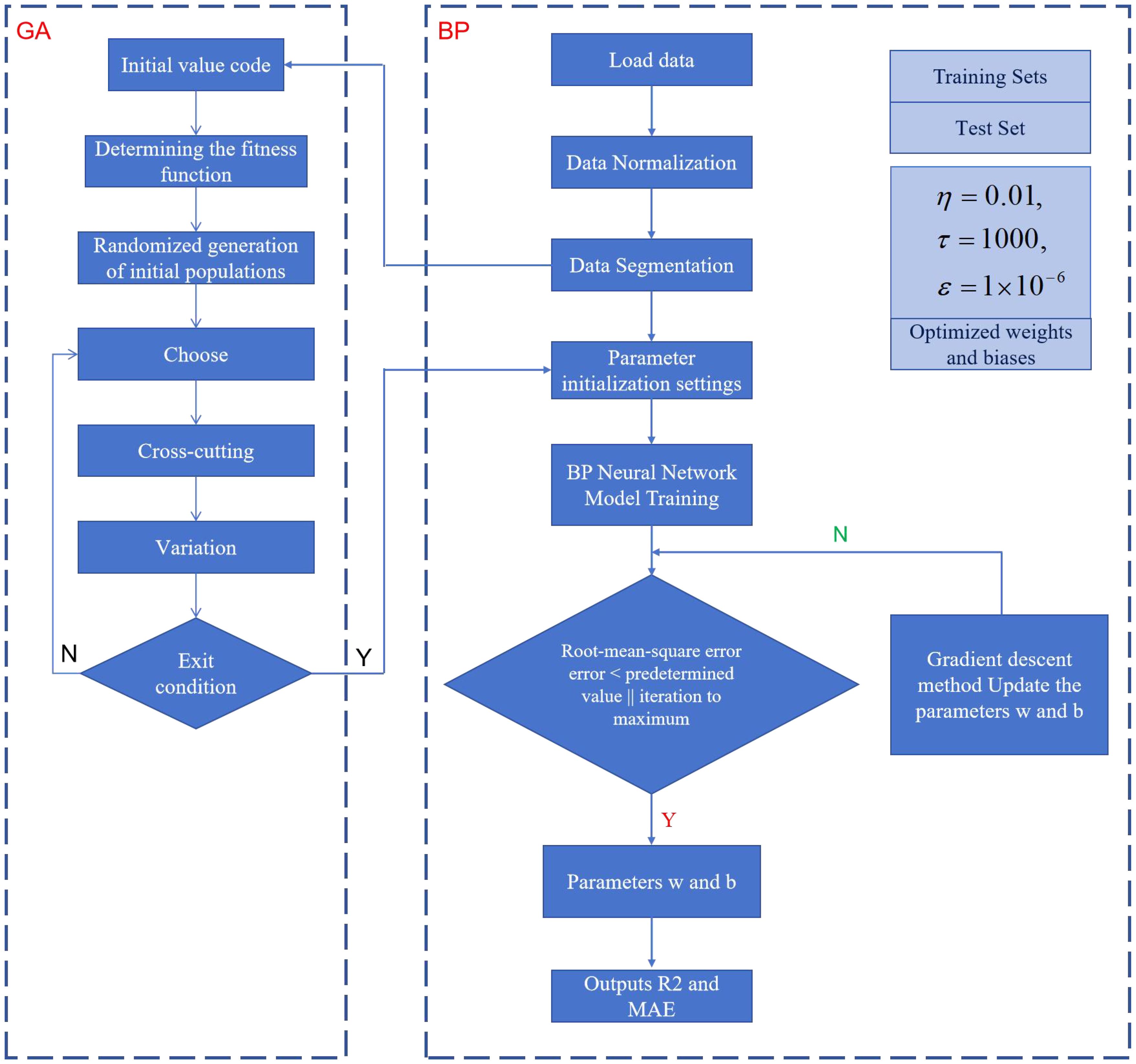
Figure 5. Flowchart of GA-BP neural network.

4.3 Aquaculture production forecasting model

Figure 6 shows the fitness curve. From Figure 6, it can be seen that the fitness gradually decreases with increasing iteration times. Figures 7 and 8 show the comparison results between the true values and the forecasting values of the training and testing sets, respectively. The R² and MAE of the training set are 0.99 and 17045, respectively, while the R² and MAE of the testing set are 0.93 and 43428, respectively. The weights and biases of the aquatic production forecasting model based on GA-BP neural network in Zhanjiang City are shown in Tables 6 and 7.

Figure 6

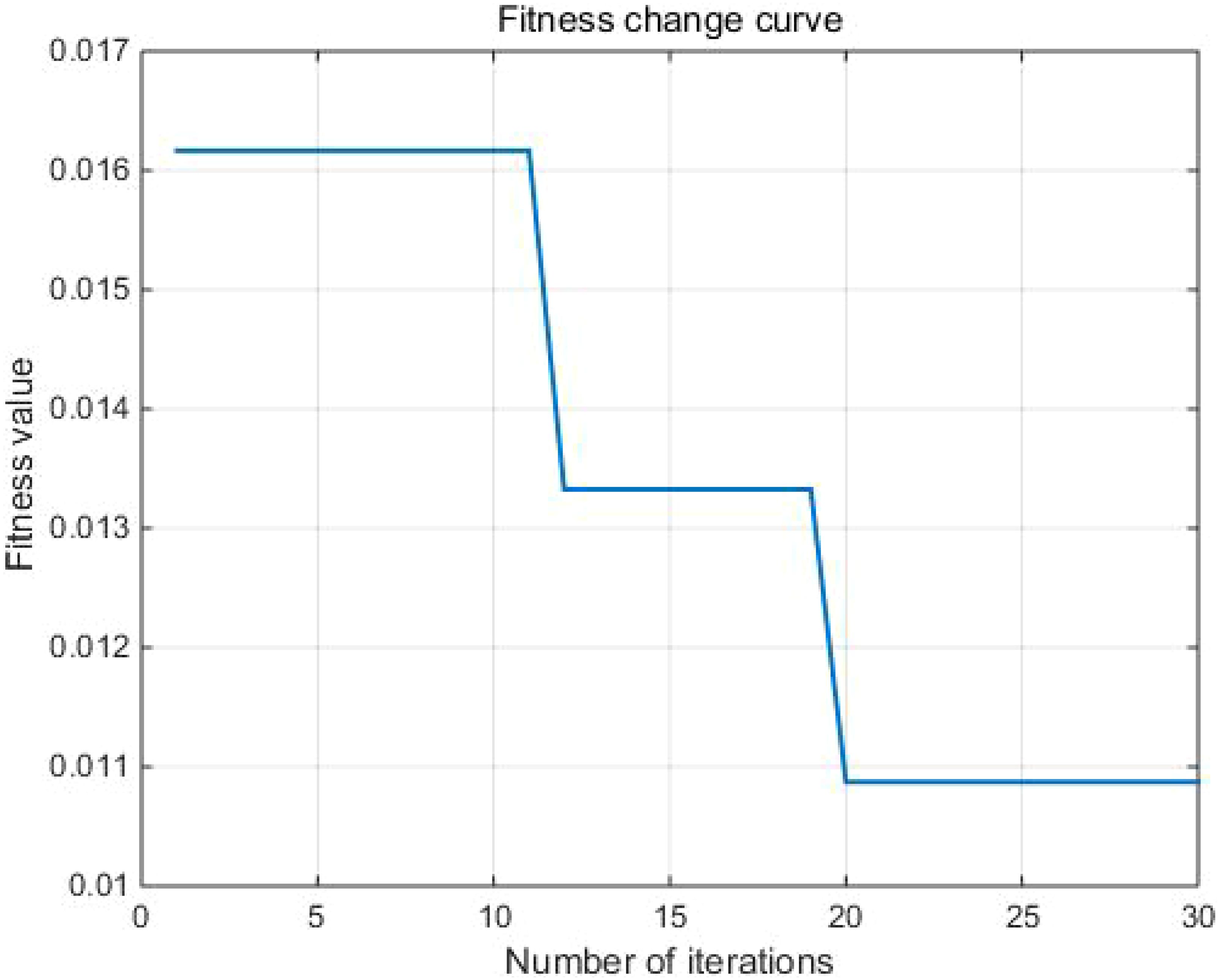
Figure 6. Fitness change curve.

Figure 7

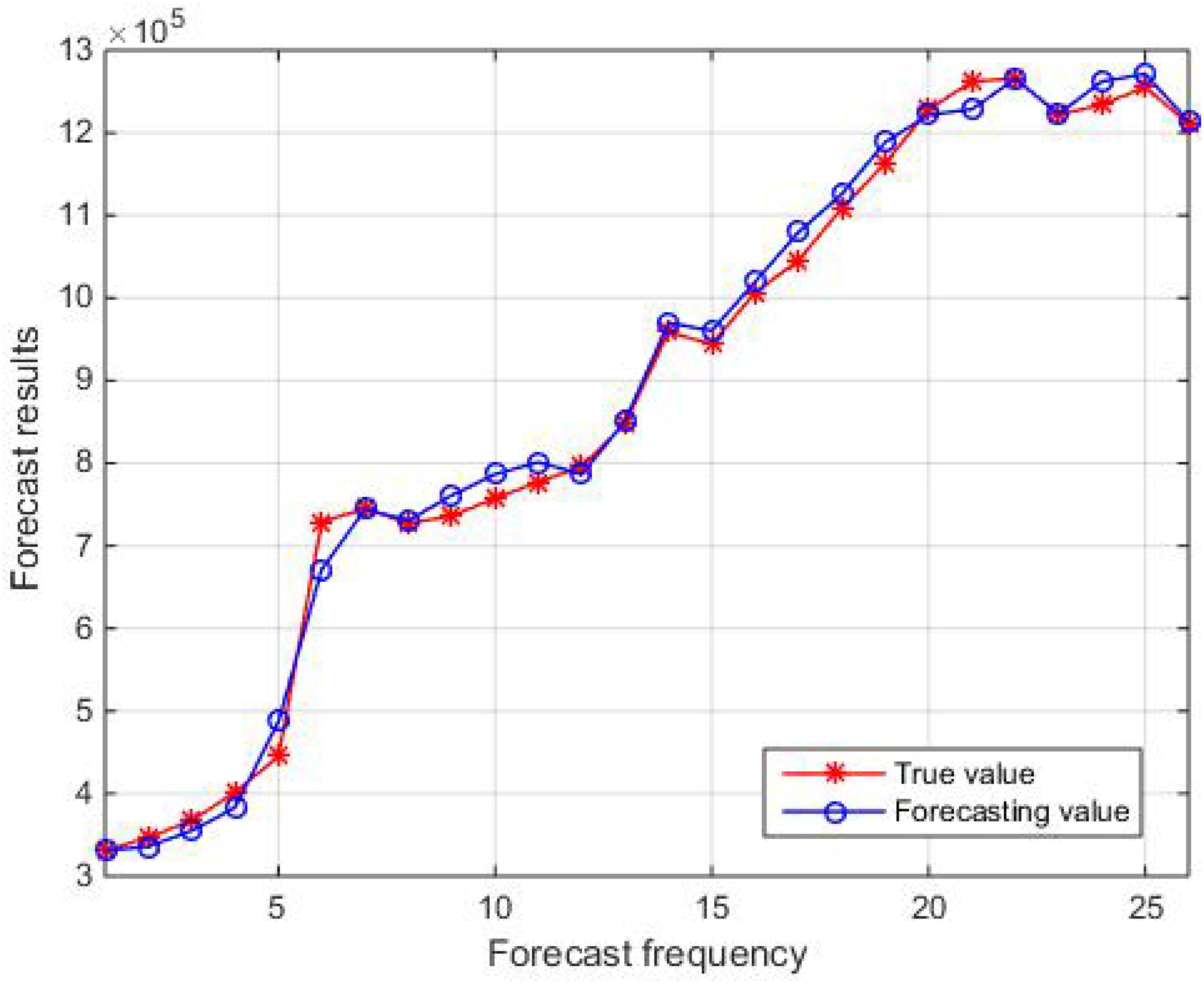
Figure 7. Comparison of true and forecasting values in the training set.

Figure 8

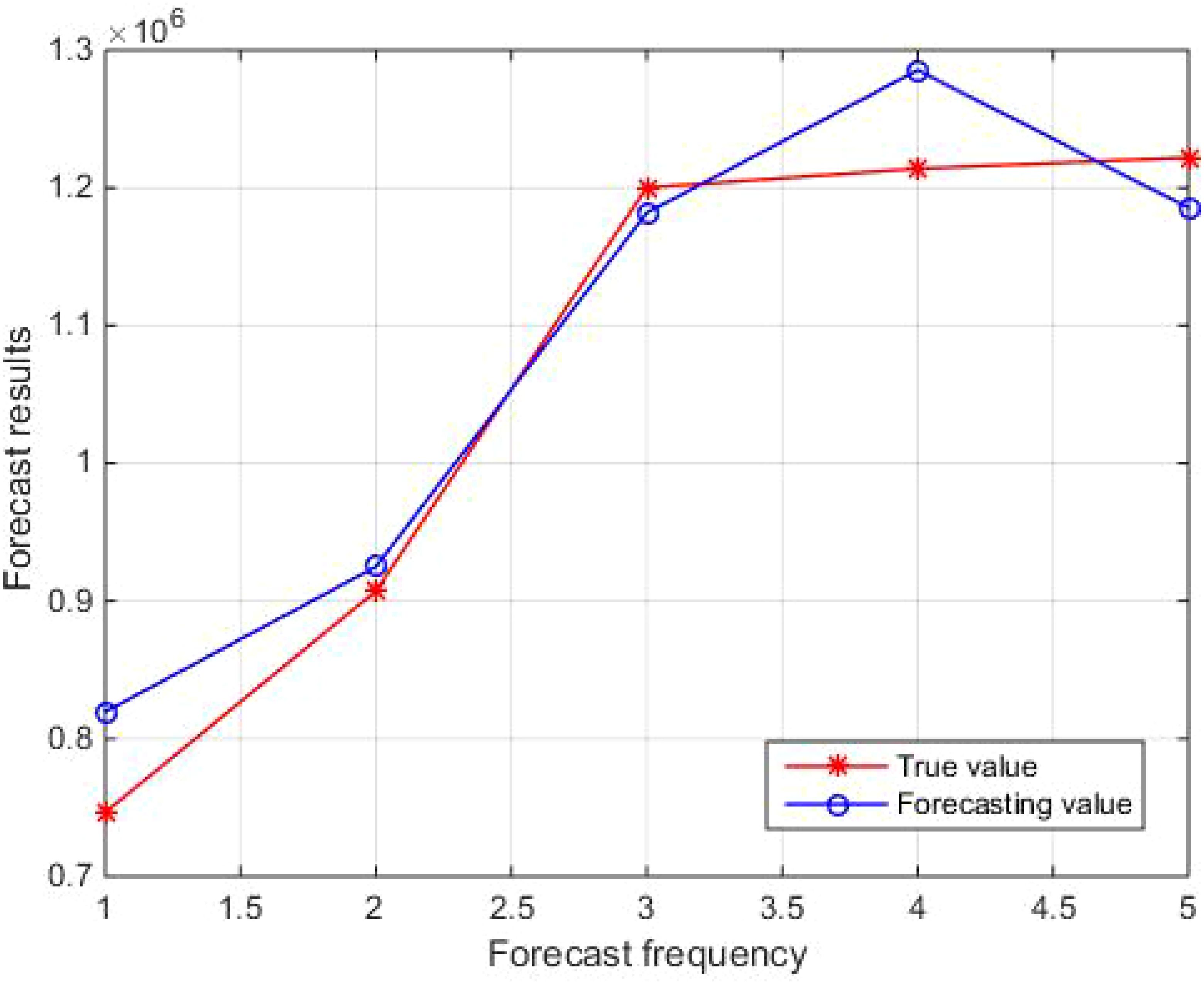
Figure 8. Comparison of true and forecasting values in the testing set.

Table 6

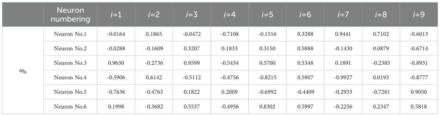
Table 6. The results of the weights (ω_ik) from the input layer to the hidden layer.

Table 7

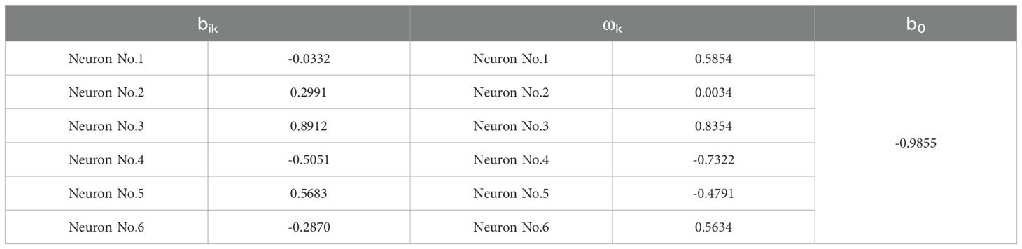
Table 7. b_ik, ω_k, and b₀ parameter table.

The above results indicate that optimizing the initial weights and biases of the BP neural network through genetic algorithm can avoid the problem of the neural network model getting stuck in local minima and causing a decrease in the accuracy and robustness of the prediction model.

However, there are also some drawbacks to using GA-BP neural networks. When dealing with large-scale datasets or complex tasks, the convergence speed of genetic algorithms may become slower. GA-BP have many parameters that need to be adjusted, such as crossover probability, mutation probability, population size, and number of iterations. The selection of these parameters has a significant impact on the performance of the algorithm. Improper parameter settings may lead to decreased algorithm performance or even the inability to find the global optimal solution. Therefore, in practical applications, a significant amount of time and effort is required to debug and optimize these parameters.

5 Aquaculture production forecasting model based on LSTM neural network

5.1 LSTM neural network

The Long Short-Term Memory (LSTM) neural network is originally proposed by Hochreiter and Schmidhuber in 1997.It is a special type of recurrent neural network (RNN) specifically designed to handle and predict long-term dependencies in sequential data. Traditional RNNs encounter issues such as vanishing or exploding gradients when processing long sequences. This primarily arises because during backpropagation, gradients can decrease or increase exponentially with the increase in time steps, making it difficult for the network to learn long-term dependencies. To address this limitation of RNNs, LSTM introduces gating mechanisms. Over time, it evolved into a framework centered around the cell state and gate structures. The network architecture of the LSTM model is illustrated in Figure 9. These gating mechanisms control the flow of information, enabling the network to remember or forget information. The cell state serves as the pathway for information transmission, allowing input information to persist through the sequence, i.e., the “memory” of the network. LSTM has three main gates: the Forget Gate, the Input Gate, and the Output Gate. The principles of LSTM are detailed on the website: https://doi.org/10.1162/neco.1997.9.8.1735.

Figure 9

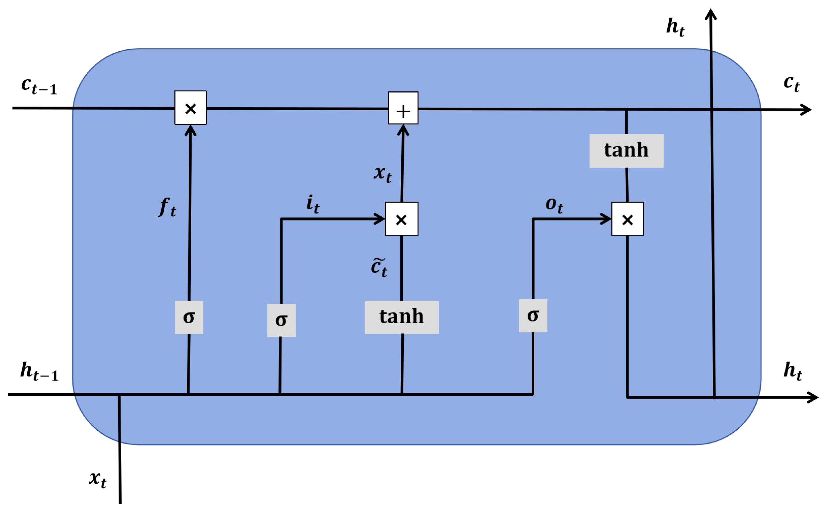
Figure 9. Network structure of the LSTM model.

The Forget Gate determines which information should be forgotten. It generates a value between 0 and 1 through a sigmoid function, representing the degree of retention for each state value. Values closer to 0 indicate that the information should be discarded, while values closer to 1 indicate that the information should be retained. The Input Gate decides which new information should be stored in the cell state. It consists of two parts: a sigmoid layer that determines which values will be updated, and a tanh layer that generates a new candidate value vector. The input of the sigmoid layer and the tanh layer of the output Gate are multiplied to obtain the updated candidate value. The Output Gate determines which parts of the current cell state will be output. It first passes through a sigmoid layer to decide which cell states will be output, then generates a candidate value for the output state through a tanh layer, and finally combines these two parts to form the final output.

Assuming that the output from the previous time step is $h_{t-1}$ and the input at the current time step is $x_t$, the computation methods for the input gate $i_t$, forget gate $f_t$, and output gate $o_t$ at the current time step are as follows, where the sigmoid function and tanh function are used as activation functions. See Equations 17-19 for details.

$\begin{array}{ll}{i}_t=\sigma (x_t{w}_{xi}+h_{t-1}{w}_{hi}+b_i)& (17)\end{array}$

$\begin{array}{ll}{f}_t=\sigma (x_t{w}_{xf}+h_{t-1}{w}_{hf}+b_f)& (18)\end{array}$

$\begin{array}{ll}{o}_t=\sigma (x_t{w}_{xo}+h_{t-1}{w}_{ho}+b_o)& (19)\end{array}$

Where $w_{xi}$, $w_{xf}$, $w_{xo}$, $w_{hi}$, $w_{hf}$ and $w_{ho}$ are weight parameters, while $w_{hi}$, $w_{hf}$, $w_{ho}$ are bias parameters.

5.2 Modeling with LSTM neural networks

The number of input features is 9, and the number of LSTM units is 4. The Adam optimization algorithm is used for gradient descent, with a maximum number of iterations set to 1500. The initial learning rate is set to 0.01, and the learning rate decay strategy is set to piecewise. This means that the learning rate will change during training according to preset rules. The learning rate decay factor is set to 0.1. When the condition for learning rate decay is met, the current learning rate will be multiplied by this factor. The learning rate decay period is set to 1200, meaning that after 1200 epochs of training, the learning rate will be multiplied by the decay factor. The dataset is shuffled at the beginning of each epoch, which helps the model generalize better and prevent overfitting.

5.3 Aquaculture production forecasting model

Figures 10 and 11 present the comparative results between the actual values and the forecasted values for the training and testing sets, respectively. The training set has an R² value of 0.998 and an MAE of 11236, whereas the testing set has an R² value of 0.94 and an MAE of 43499.The R² value of LSTM is closer to 1 and its MAE value is smaller compared to GA-BP, indicating that the differences between the predicted values and the true values are generally smaller, and the fitting effect is better than that of GA-BP.

Figure 10

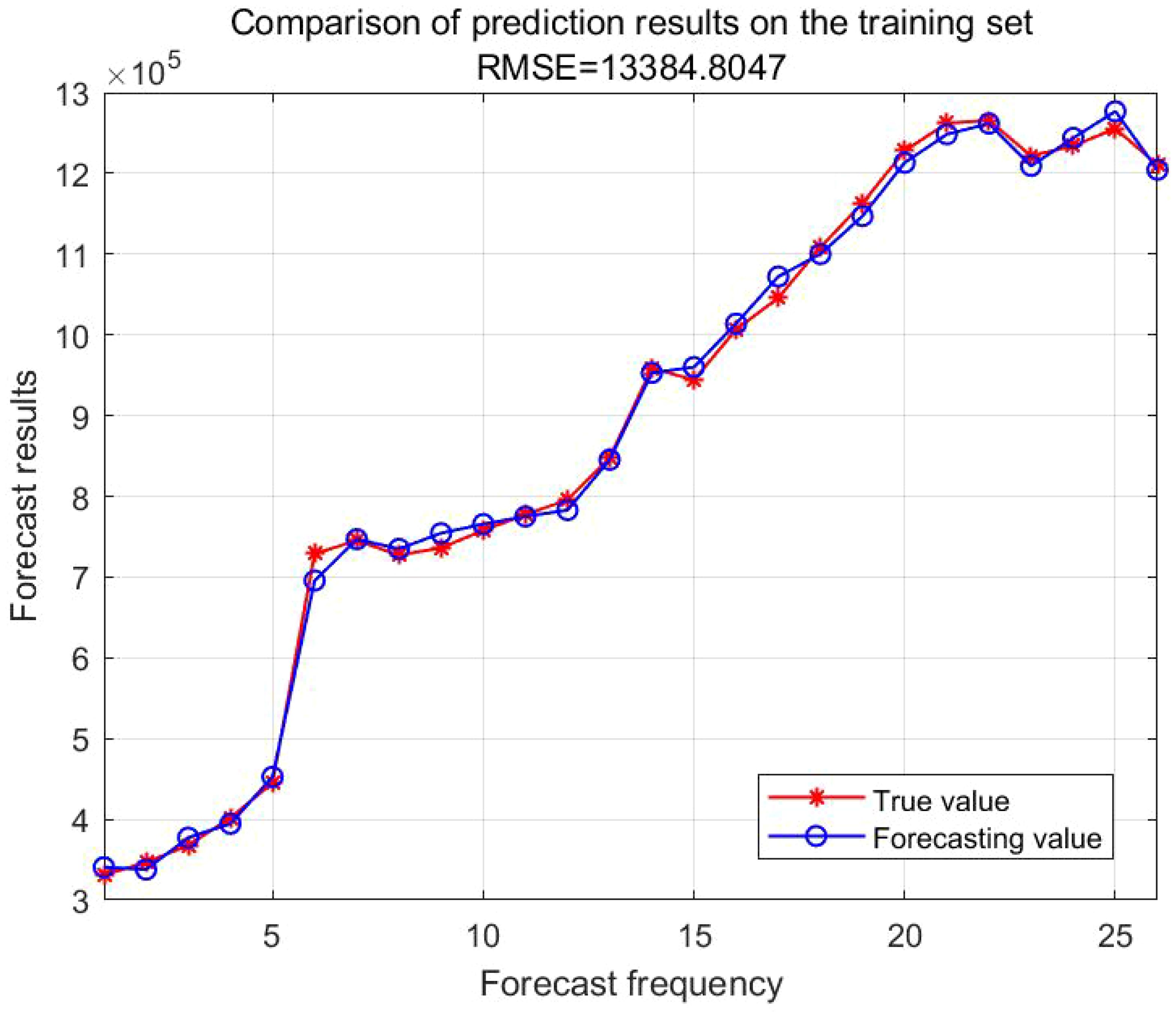
Figure 10. Comparison of true and forecasting values in the training set.

Figure 11

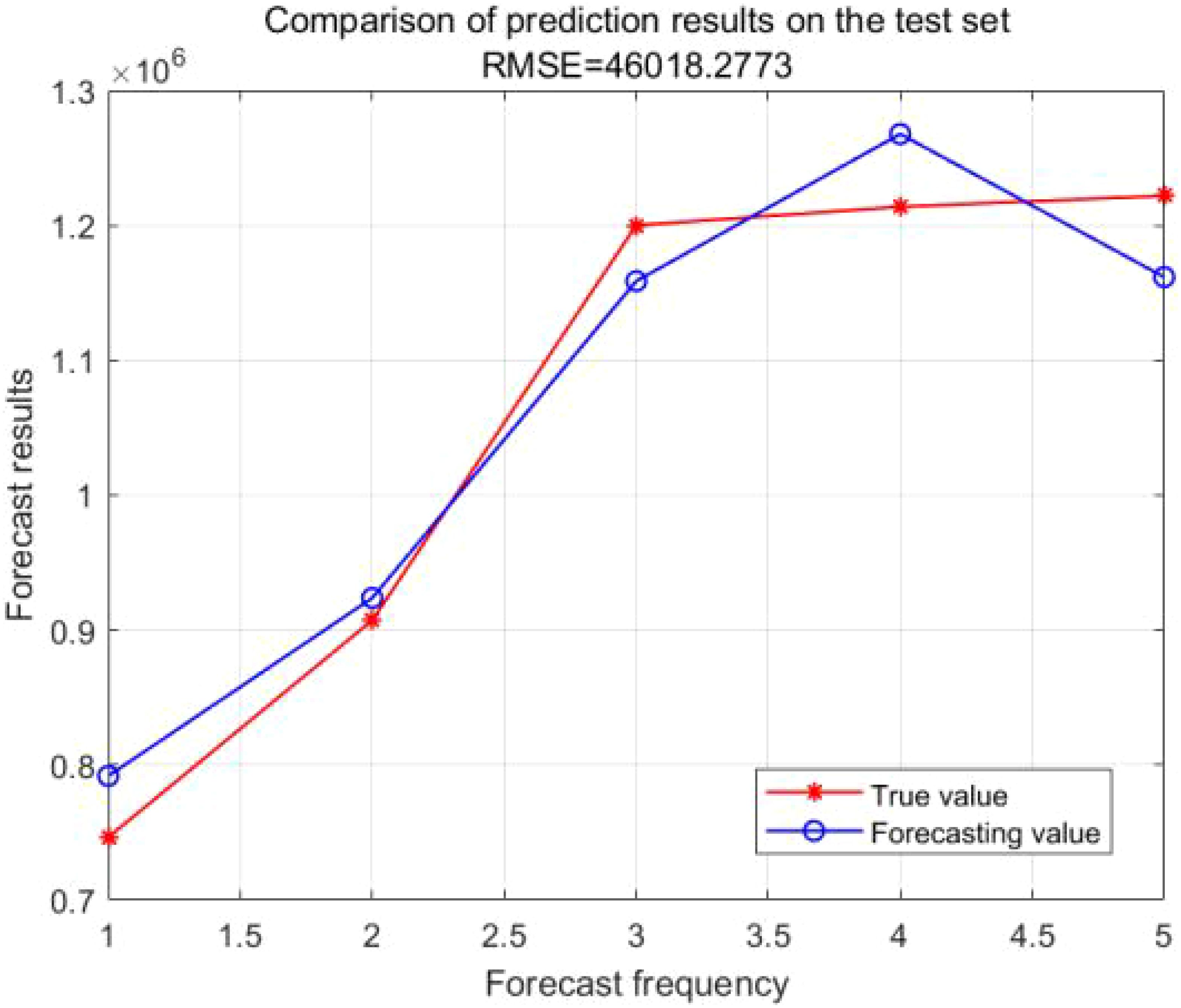
Figure 11. Comparison of true and forecasting values in the testing set.

6 Aquaculture production forecasting model based on RBF neural network

6.1 RBF neural network

In terms of function approximation, the BP neural network employs the negative gradient descent method, which belongs to global approximation. Consequently, it has issues such as slow convergence speed and being prone to falling into local minima, resulting in significant errors in prediction problems. The Radial Basis Function (RBF) is a neural network architecture proposed by J. Moody and C. Darken in the late 1980s. The RBF neural network achieves a nonlinear mapping relationship between input data and output data by constructing radial basis functions (typically Gaussian functions). It has the capabilities of optimal approximation and overcoming local minima problems. The structure of RBF neural network is shown in Figure 12.

Figure 12

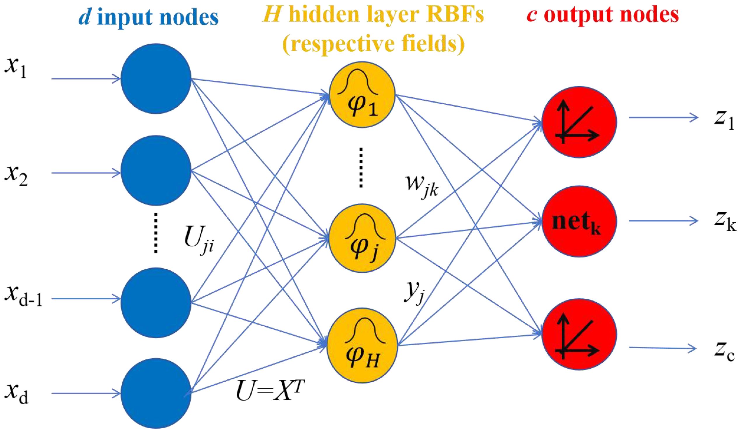
Figure 12. The schematic diagram of the Radial Basis Function (RBF) neural network.

6.2 RBF neural network operation steps

Taking 9 influencing factors of aquatic product yield as inputs, where d=9 in the Figure 13, the relationship between the input layer and the hidden layer is a nonlinear mapping, and the basis function is a Gaussian function.

Figure 13

Figure 13. Comparison of true and forecasting values in the training set.

$\begin{array}{ll}{R}_i(x)=exp[-\frac{{\Vert x-c_i\Vert }^2}{2{\sigma }_i^2}]& (20)\end{array}$

Among them, i=1,2,…,m; x is an n-dimensional input vector. $\Vert x-c_i\Vert$ denotes the vector norm, representing the distance between x and $c_i$; the value $R_i(x)$ of Gaussian function attains its unique maximum at the center of a certain basis function. According to the Equation 20, as $\Vert x-c_i\Vert$ increases, the value of the basis function $R_i(x)$ decreases until it approaches zero. For a given input value x, only a small portion near the center of x is activated. In the Gaussian function, $c_i$ represents the center value of the ith basis function, which has the same dimensionality as the input vector and is obtained based on the K-Means clustering method. The specific steps are as follows:

6.2.1 Network initialization

Randomly select h training samples as the clustering centers $c_i$ (i=1,2,…,h).

6.2.2 Grouping the input training sample set according to the nearest neighbor rule

Assign x_p to the respective clustering set ${\vartheta }_p$ (p=1,2,…,p) based on the Euclidean distance between x_p and the center $c_i$.

6.2.3 Readjust the clustering centers

Calculate the average value of the training samples in each clustering set p, which is the new clustering center $c_i$. If the new clustering centers no longer change, the obtained $c_i$ are the final basis function centers for the RBF neural network. Otherwise, return to step (2) for the next round. In the Gaussian function, ${\sigma }_i$ represents the standardization constant for the width of the ith basis function center. It can be solved by calculation Equation 21:

$\begin{array}{ll}{\sigma }_i=\frac{c_{max}}{\sqrt{2h}},i=1,2,\dots h& (21)\end{array}$

Where $c_{max}$ represents the maximum distance between the selected centers. The connection weights between the hidden layer and the output layer can be directly calculated using the least squares method, with the calculation Equation 22:

$\begin{array}{ll}w=exp(\frac{h}{c_{max}^2}{\Vert x_p-c_i\Vert }^2),p=1,2,\dots p;i=1,2,\dots h& (22)\end{array}$

The spreading speed of the radial basis function is set to 1000.

6.3 Aquaculture production forecasting model

Figures 13 and 14 present the comparative results between the actual values and the forecasted values for the training and testing sets, respectively. The training set has an R² value of 0.999 and an MAE of 5460, whereas the testing set has an R² value of 0.96 and an MAE of 27725.

Figure 14

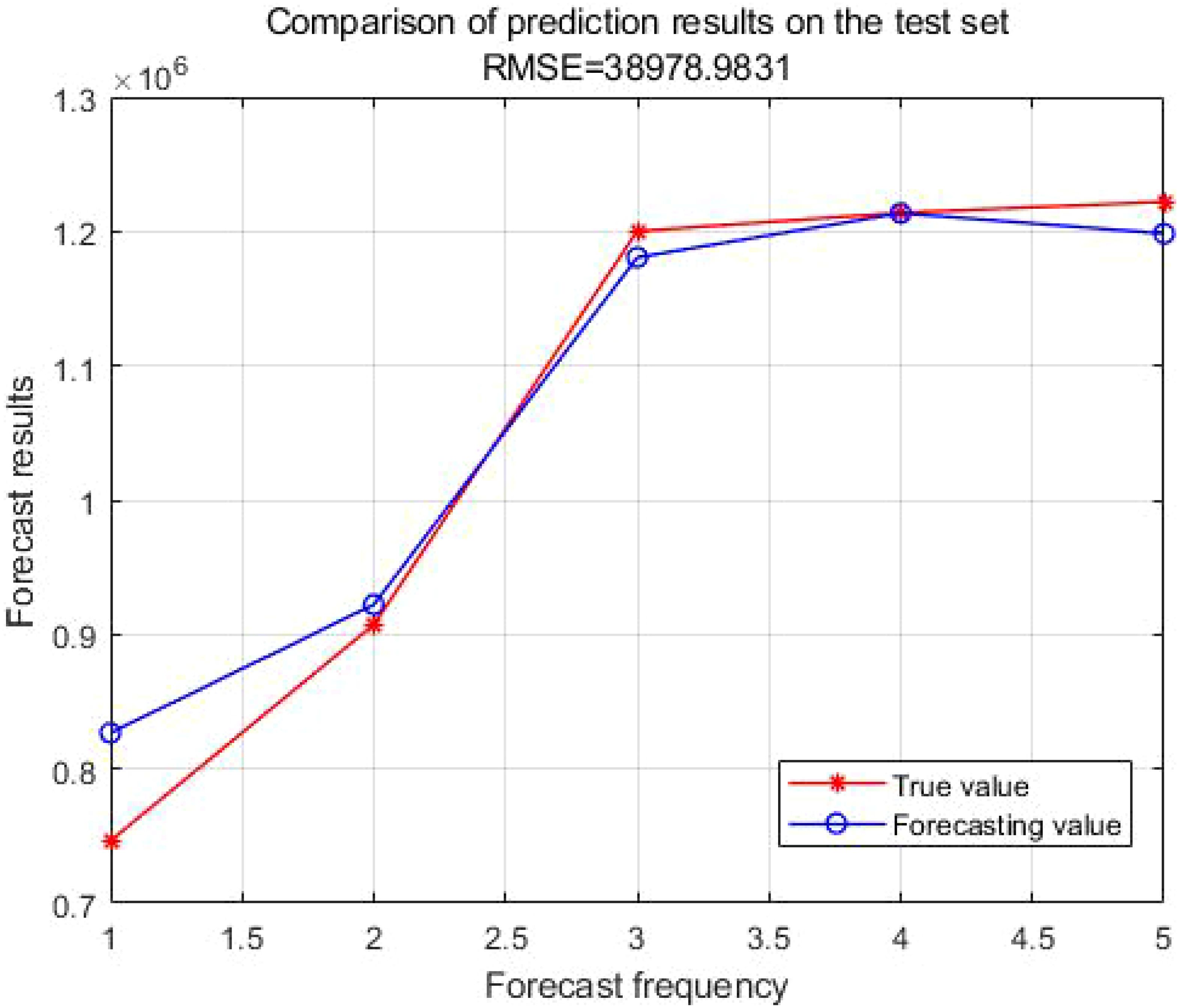
Figure 14. Comparison of true and forecasting values in the testing set.

7 Model comparison

The Table 8 presents the performance of four neural network models (BP, GA-BP, LSTM, and RBF) on both training and testing datasets. For the BP neural network on the training set:The R² value is 0.92, indicating a high degree of fit on the training data. The MAE is 73,700, representing an average absolute error between predicted and actual values of 73,700.On the testing set, the R² drops to 0.73, suggesting poor generalization ability on unseen data, indicative of significant overfitting. The MAE increases to 92,995, indicating larger prediction errors on the testing set. For the GA-BP neural network on the training set:The R² value improves to 0.99, indicating a very high degree of fit on the training data. The MAE significantly decreases to 17,045, with a notable reduction in prediction error. On the testing set, the R² is 0.93, showing a significant improvement compared to the BP neural network’s performance on the testing set, indicating stronger generalization ability of the GA-BP model. The MAE is 43,428, which, although still indicating some error, is substantially lower than that of the BP neural network. For the LSTM neural network on the training set:The R² value is as high as 0.998, indicating nearly perfect fit on the training data. The MAE is 11,236, representing very small prediction errors. On the testing set, the R² is 0.94, indicating strong generalization ability of the LSTM model on the testing set. The MAE is 43,499, slightly higher than that of GA-BP on the testing set, but considering LSTM’s advantages in processing time series data, this level of error is still acceptable. For the RBF neural network on the training set:The R² value is nearly perfect at 0.999, indicating a very high degree of fit on the training data. The MAE is 5,460, representing very small prediction errors. On the testing set, the R² is 0.96, indicating strong generalization ability of the RBF model. The MAE is 27,725, the smallest among the four models on the testing set, demonstrating the RBF model’s excellent performance in prediction accuracy. So, RBF neural network has the highest accuracy and best robustness in predicting aquatic production.

Table 8

Table 8. Comparison of forecasting models based on BP, GA-BP, LSTM and RBF neural network.

Figure 15 displays the time series prediction comparison plot, Figure 16 presents the bootstrap confidence interval plot, Figure 17 illustrates the error distribution boxplot, Figure 18 shows the annual error trend analysis, Figure 19 demonstrates the model performance ranking chart, Figure 20 exhibits the model performance benchmark plot, and Figure 21 reveals the residual diagnostic plots. To comprehensively address concerns regarding dataset limitations and model robustness, our multi-modal analysis demonstrates RBF’s consistent superiority through seven key visualizations: (1) The time series prediction comparison plot (Figure 15) reveals RBF’s precise tracking of actual production trends across the entire 1992–2022 period, particularly in the 2018–2022 test window; (2) Bootstrap confidence interval plots (Figure 16) confirm RBF’s stability (R²=0.960 ± 0.246) through 1000 resampling iterations, showing 46% lower variability than BP; (3) Error distribution boxplots (Figure 17) quantify RBF’s exceptional test-set consistency (IQR=5.6% vs BP’s 18.3%); (4) Annual error trend analysis (Figure 18) demonstrates RBF’s sustained [-5%,+15%] error bounds throughout climatic and economic fluctuations; (5) The model performance ranking chart (Figure 19) definitively positions RBF as top-performer (test R²=0.960>LSTM’s 0.940); (6) Performance benchmark plots (Figure 20) highlight RBF’s minimal generalization gap (ΔR²=0.039) and lowest test MAE (27,725 tons); while (7) residual diagnostic plots (Figure 21) validate RBF’s statistically robust error structure (σ=17.4, no heteroscedasticity). Collectively, this evidence chain-spanning temporal accuracy, statistical stability, error characteristics, and ranking metrics-conclusively establishes RBF as the optimal architecture for small-sample aquatic production forecasting.

Figure 15

Figure 15. (a, b) Time series prediction comparison plot.

Figure 16

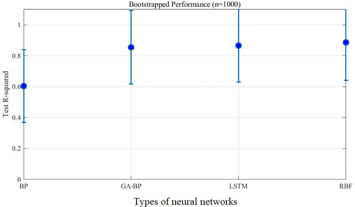
Figure 16. Bootstrap confidence interval plot.

Figure 17

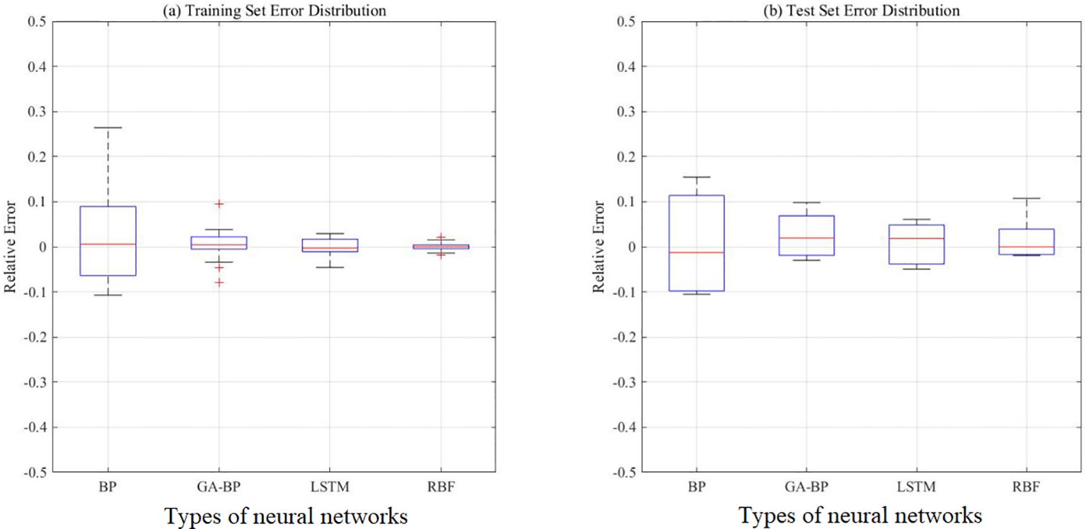
Figure 17. (a, b) Error distribution boxplot.

Figure 18

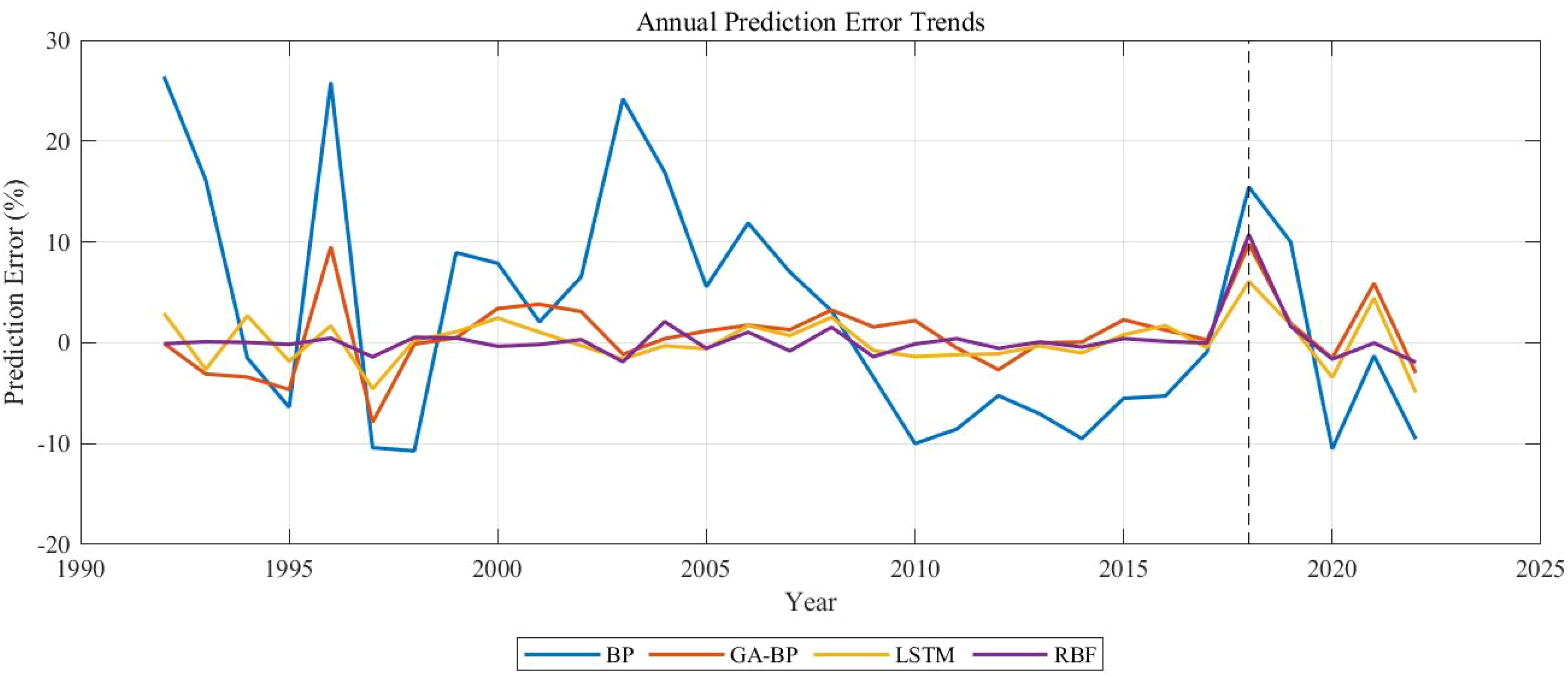
Figure 18. Annual error trend analysis.

Figure 19

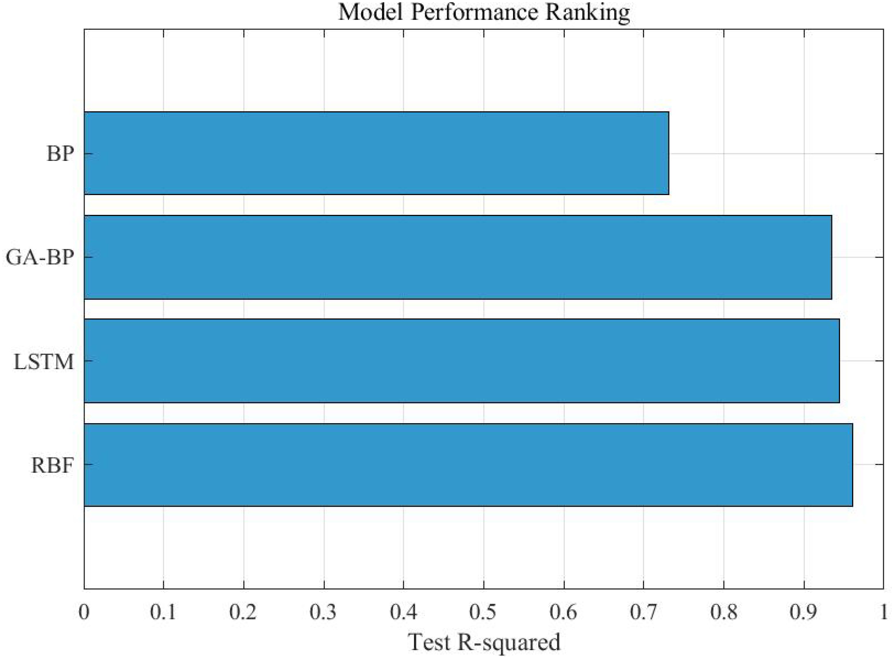
Figure 19. Model performance ranking chart.

Figure 20

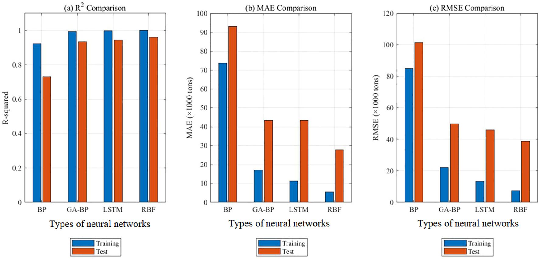
Figure 20. (a-c) Model performance benchmark plot.

Figure 21

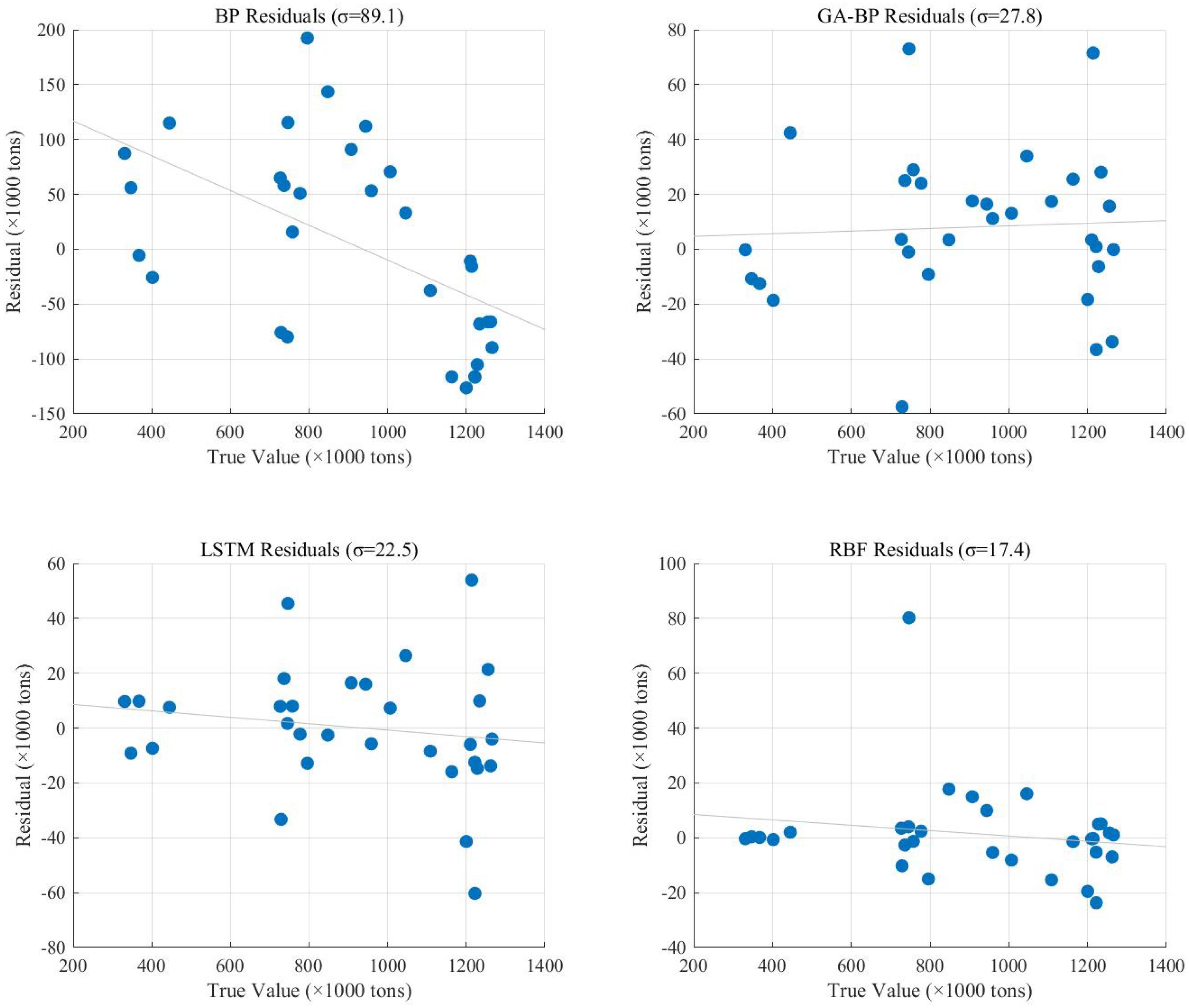
Figure 21. Residual diagnostic plots.

The superior performance of the RBF neural network over LSTM in this study can be attributed to several key factors that are closely related to the characteristics of the available dataset and the nature of aquaculture production systems. It should be noted that the 31-year time series (1992-2022) represents the most extensive temporal coverage currently available for Zhanjiang’s aquaculture production records, which inherently limits the complexity of models that can be effectively applied. The annual resolution of this dataset is found to be better suited to RBF’s localized approximation capabilities than to LSTM’s sequential learning strengths. While LSTM networks are typically effective for modeling complex temporal dependencies in high-frequency data, the year-to-year variations in aquaculture production are observed to be influenced more by aggregated environmental and socioeconomic conditions than by intricate sequential patterns. This fundamental characteristic of the data explains why the simpler RBF architecture achieves better performance. The RBF network’s design is demonstrated to be particularly appropriate for this application, as its fewer parameters make it less susceptible to overfitting when trained on limited data-a crucial advantage given the relatively small dataset available for this regional study. Furthermore, the RBF network’s ability to model stable, nonlinear relationships between input variables and production output is shown to align well with the gradual trends that characterize multi-year aquaculture production data. Sensitivity analysis confirms the dominance of static factors in predicting annual production, with variables such as GDP per capita and aquaculture area being identified as having greater predictive power than purely time-dependent features. This finding provides a clear explanation for why RBF’s strength in modeling static nonlinear mappings proves more effective than LSTM’s sequential learning capabilities for this specific forecasting task. Although LSTM achieves excellent performance on the training set, a slightly larger generalization gap is observed compared to RBF, suggesting that the additional complexity of the LSTM architecture may not be justified given the available data. These results are consistent with established principles in machine learning applications, where traditional methods are frequently found to outperform more complex architectures when working with limited training samples. The practical implications are significant for aquaculture management, as they demonstrate that reliable production forecasting can be achieved without resorting to resource-intensive deep learning approaches, particularly when working with the longest available but still limited time series data typical of regional production records.

8 Parameter sensitivity analysis

Based on the weight and bias data of GA-BP neural network, this paper adopts the parameter sensitivity analysis method proposed by Zhang and Goh (2018) to analyze the relative importance of factors affecting aquatic production in Zhanjiang. The contribution of each factor to aquatic production is obtained. The principle of the parameter sensitivity analysis method is shown in the following equation. See Equations 23-27 for details.

$\begin{array}{ll}{A}_{.k}={\displaystyle {\sum }_{i=1}^5\left|{\omega }_{ik}\times b_{ik}\right|}& (23)\end{array}$

$\begin{array}{ll}{b}_{ik.}=\frac{\left|{\omega }_{ik}\times b_{ik}\right|}{A_{.k}}& (24)\end{array}$

$\begin{array}{ll}{C}_{i.}={\displaystyle {\sum }_{k=1}^7{b}_{ik}}& (25)\end{array}$

$\begin{array}{ll}D=\max (C_{i.})& (26)\end{array}$

$\begin{array}{ll}{S}_{i.}=\frac{C_{i.}}{D}\times 100\%& (27)\end{array}$

Figure 22 shows the results of parameter sensitivity analysis. The influencing factors 1–9 represent, in order, the total aquaculture area, the number of motorized fishing boats, the fishery population, the temperature, the sunshine duration, the Engel’s coefficient, the consumer price index, the household registered population, and the per capita GDP. It can be seen from Figure 22 that the most important factor affecting aquaculture output is per capita GDP, followed by sunshine hours, Engel coefficient, consumer price index, temperature, fishery population, total area of aquaculture, total registered residence population and number of motorized fishing boats.

Figure 22

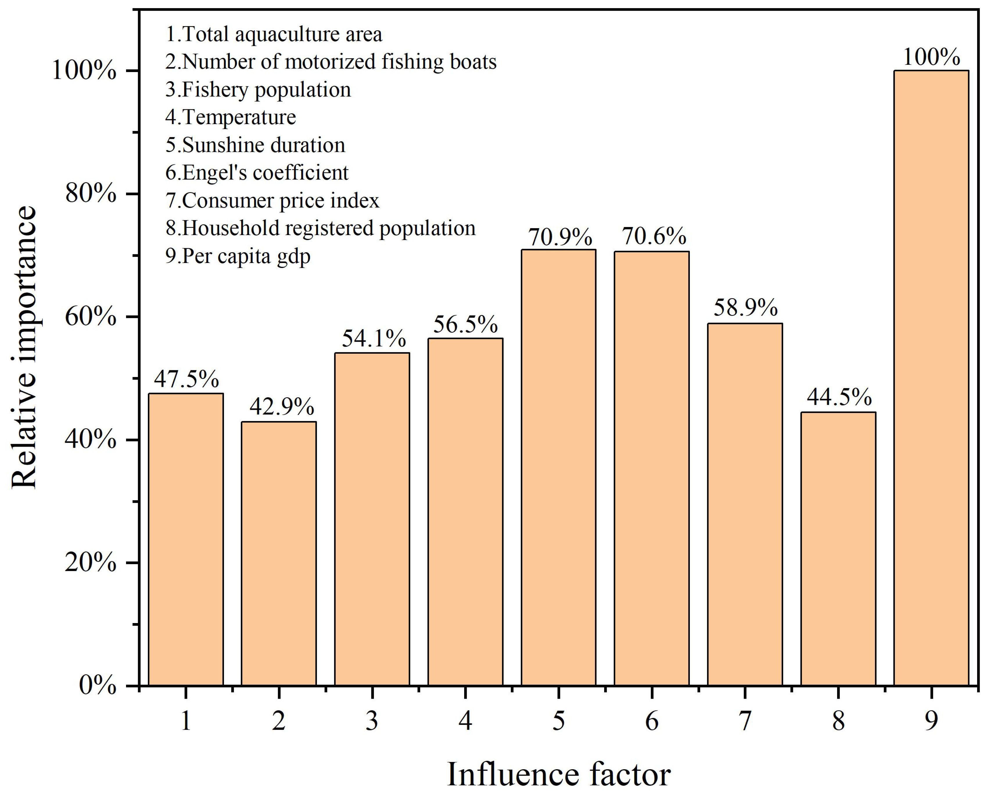
Figure 22. Parameter sensitivity analysis results.

9 Conclusion

To forecast the aquatic production in Zhanjiang City, this paper establishes a forecasting model for aquatic production by integrating the advantages of GRA, GA, and BP neural network. Subsequently, the theory of parameter sensitivity analysis is employed to quantitatively determine the contribution of each influencing factor to the aquatic production. The main conclusions of this paper are as follows:

1. The GRA can effectively quantify the appropriateness of the selection factors that affect aquatic production.

2. After optimizing the BP neural network by GA, the accuracy and robustness of the aquatic production forecasting model are significantly improved, with the R2 increasing from 0.73 to 0.93 and the MAE decreasing from 92995 to 43428 in the test set.

3. Compared with BP neural network, GA-BP neural network, and LSTM, the RBF neural network model has the highest forecast accuracy and the most advantage in robustness. So, when establishing a forecast model for aquatic production, RBF is the optimal choice.

4. The most significant factor affecting the aquaculture output is per capita GDP, followed by sunshine hours, Engel coefficient, consumer price index, temperature, fishery population, total area of aquaculture, total registered residence population and number of motorized fishing boats.

Data availability statement

The raw data supporting the conclusions of this article will be made available by the authors, without undue reservation.

Author contributions

JH: Writing – original draft, Conceptualization. JY: Data curation, Writing – original draft. CY: Investigation, Writing – original draft. YZ: Visualization, Software, Writing – original draft. CL: Formal Analysis, Writing – review & editing, Conceptualization, Data curation, Investigation, Methodology, Software.

Funding

The author(s) declare that financial support was received for the research and/or publication of this article. This work was supported by the Non funded Science and Technology Research and Development Program of Zhanjiang City (Grant NO. 2024B01115), the program for scientific research start-up funds of Guangdong Ocean University(Grant NO. 060302072305), the Fund of Guangdong Provincial Key Laboratory of Intelligent Equipment for South China Sea Marine Ranching (Grant NO. 2023B1212030003) and the Non funded Science and Technology Research and Development Program of Zhanjiang City (Grant NO. 2024B01002).

Conflict of interest

The authors declare that the research was conducted in the absence of any commercial or financial relationships that could be construed as a potential conflict of interest.

Generative AI statement

The author(s) declare that no Generative AI was used in the creation of this manuscript.

Any alternative text (alt text) provided alongside figures in this article has been generated by Frontiers with the support of artificial intelligence and reasonable efforts have been made to ensure accuracy, including review by the authors wherever possible. If you identify any issues, please contact us.

Publisher’s note

All claims expressed in this article are solely those of the authors and do not necessarily represent those of their affiliated organizations, or those of the publisher, the editors and the reviewers. Any product that may be evaluated in this article, or claim that may be made by its manufacturer, is not guaranteed or endorsed by the publisher.

References

Anthony Koslow J. and Davison P. C. (2016). Productivity and biomass of fishes in the California Current Large Marine Ecosystem: Comparison of fishery-dependent and -independent time series. Environ. Dev. doi: 10.1016/j.envdev.2015.08.005

Crossref Full Text | Google Scholar

Benavides I. F., Romero-Leiton J., Santacruz M., Barreto C., Puentes V., and Selvaraj J. J. (2022). Applying seasonal time series modeling to forecast marine fishery landings for six species in the Colombian Pacific Ocean. Regional Stud. Mar. Sci. 56, 102716. doi: 10.1016/j.rsma.2022.102716

Crossref Full Text | Google Scholar

Cho Y. (2006). Time series analysis of general marine fisheries. J. Rural Development/Nongchon-Gyeongje 1).

Google Scholar

Deng J. (1990). Tutorial on Grey System Theory. (Wuhan: Huazhong University of Science and Technology Press).

Google Scholar

Ghani I. M. M. and Ahmad S. (2010). Stepwise multiple regression method to forecast fish landing. Procedia-Social Behav. Sci. 8, 549–554. doi: 10.1162/neco.1997.9.8.1735

PubMed Abstract | Crossref Full Text | Google Scholar

Jasmin S. A., Ramesh P., and Tanveer M. (2022). An intelligent framework for prediction and forecasting of dissolved oxygen level and biofloc amount in a shrimp culture system using machine learning techniques. Expert Syst. Appl. 199.

Google Scholar

Jaureguizar A. J., Cortes F., Maiztegui T., Camiolo M. D., and Milessi A. C. (2024). Unraveling the environmental influence on inter-annual fishery yield in a small-scale gillnet fishery under Rio de la Plata influence, South America. Estuar. Coast. shelf Sci. 303. doi: 10.1016/j.ecss.2024.108795

Crossref Full Text | Google Scholar

Kalhoro M. A., Liu Q., Zhu L. X., Jiang Z., and Liang Z. (2024). Assessing fishing capacity of two tuna fish species using different time-series data in Pakistan, Northern Arabian Sea. Estuarine Coast. Shelf Sci. 299, 108692. doi: 10.1016/j.ecss.2024.108692

Crossref Full Text | Google Scholar

Law R., Li G., Fong D. K. C., and Han X. (2019). Tourism demand forecasting: A deep learning approach. Ann. Tourism Res. 75, 410–423. doi: 10.1016/j.annals.2019.01.014

Crossref Full Text | Google Scholar

Miguéis V. L., Pereira A., Pereira J., and Figueira G. (2022). Reducing fresh fish waste while ensuring availability: Demand forecast using censored data and machine learning. J. Cleaner Production. doi: 10.1016/j.jclepro.2022.131852

Crossref Full Text | Google Scholar

Naorem O. S., Kumar P., Bhar L. M., Singh K. N., Singh P., Naorem O. S., et al. (2013). Forecasting of fish production from ponds – a nonlinear model approach. Indian J. Fisheries 60, 67–71.

Google Scholar

Panwar S., Kumar A., Singh K., Sarkar S., Gurung B., and Rathore A. (2018). Growth modelling and forecasting of common carp and silver carp in culture ponds: A re-parametrisation approach. Indian J. Fisheries.

Google Scholar

Quetglas A., Ordines F., and Guijarro B. (2011). The Use of Artificial Neural Networks (ANNs) in Aquatic Ecology (Spain: Instituto Español de Oceanografía, Centre Oceanogràfic de les Balears).

Google Scholar

Rahman L. F., Marufuzzaman M., Alam L., Bari M. A., Sumaila U. R., and Sidek L. M. (2021). Developing an ensembled machine learning prediction model for marine fish and aquaculture production. Sustainability 13. doi: 10.3390/su13169124

Crossref Full Text | Google Scholar

Raman R. K., Sathianandan T. V., Sharma A. P., Sathianandan T. V., Sharma A. P., and Mohanty B. P. (2017). Modelling and forecasting marine fish production in odisha using seasonal ARIMA model. Natl. Acad. Sci. Lett. 40. doi: 10.1007/s40009-017-0581-2

Crossref Full Text | Google Scholar

Siddique M. A. B., Mahalder B., Haque M. M., Shohan H. M., Biswas J. C., Akhtar S., et al. (2024). Corrigendum to “Forecasting of Tilapia (Oreochromis niloticus) production in Bangladesh using ARIMA model. Heliyon 10. doi: 10.1016/j.heliyon.2024.e27111

PubMed Abstract | Crossref Full Text | Google Scholar

Stephen S., Yadav V. K., and Kumar R. (2022). Comparative study of statistical and machine learning techniques for fish production forecasting in Andhra Pradesh under climate change scenario. Indian J. Geo-Marine Sci.

Google Scholar

Tan X. R. and Deng J. L. (1995). Grey relational analysis: A new method for multifactor statistical analysis. Stat. Res.

Google Scholar

Tsitsika E. V., Maravelias C. D., and Haralabous J. (2010). Modeling and forecasting pelagic fish production using univariate and multivariate ARIMA models. Fisheries Sci. 73, 979–988. doi: 10.1111/j.1444-2906.2007.01426.x

Crossref Full Text | Google Scholar

Zhang W. and Goh A. T. C. (2018). Assessment of soil liquefaction based on capacity energy concept and back-propagation neural networks. Integrating Disaster Sci. Manage., 41–51. doi: 10.1016/B978-0-12-812056-9.00003-8

Crossref Full Text | Google Scholar

Zhao S., Zhang S., Liu J., Wang H., and Zhao R. (2021). Application of machine learning in intelligent fish aquaculture: A review. Aquaculture 540, 736724. doi: 10.1016/j.aquaculture.2021.736724

Crossref Full Text | Google Scholar