The three-dimensional composite analysis method of mesoscale eddies in the Philippine Sea based on sound speed profile clustering

Traditional composite methods for mesoscale eddies predominantly employ simplistic geographical partitioning, seldom taking into account the variations in mesoscale eddy structures that are jointly influenced by seasonal and regional factors within the area., nor does it consider the issue of approximating mesoscale eddies as elliptical structures. This study combines mesoscale eddy data from satellite altimetry (2007-2022) with Argo profile data captured by eddies to propose a mesoscale eddy composite analysis method based on profile clustering and an elliptical model. This method provides the three-dimensional structures of various types of mesoscale eddies in the Philippine Sea. The results show that the eccentricity of the best-fitting ellipses for mesoscale eddies in the Philippine Sea is predominantly between 0.7 and 0.9, with the orientation of the major axis mostly directed at 80° northeast. Based on sound speed profile clustering, mesoscale eddies are classified into five categories. The composite eddy anomaly structures exhibit a clear correlation with the profile types. Compared to the single mesoscale eddy structure obtained by the traditional mesoscale eddy composite method, this approach accurately composites five typical mesoscale eddy structures in the Philippine Sea, and its elliptical shape is more consistent with actual observational results.

1 Introduction

Mesoscale eddies are ubiquitous and have significant impacts on many geophysical oceanographic parameters (Ma et al., 2024; Xu et al., 2024). Water masses trapped by mesoscale eddies can travel long distances while retaining their original temperature and salinity characteristics (Chen et al., 2022). The generation of mesoscale eddies is spatially heterogeneous, and it is closely related to the unique dynamic structures and water mass compositions of each region (Chaigneau et al., 2011; Sun et al., 2017). Therefore, investigating the three-dimensional structures of mesoscale eddies in different regions is of paramount importance.

In the North Pacific, strong eddy kinetic energy is concentrated in two latitudinal bands: one near the Kuroshio Extension, and another in the northwestern Pacific subtropical region near the Philippine Sea (Qiu and Chen, 2010; Chen et al., 2022). Studies show that the circulation in the northwestern Pacific near the Philippine Sea plays a crucial role in global thermohaline transport and climate dynamics (Hu et al., 2015). Moreover, due to the combined effects of baroclinic and barotropic instabilities in the region, the Philippine Sea is one of the areas with the largest eddy energy in the northwestern Pacific, second only to the Kuroshio Extension (Qiu, 1999; Zheng et al., 2015). As a result, this study focuses on the mesoscale eddies in the vicinity of the Philippine Sea.

In recent years, the three-dimensional structure of mesoscale eddies and their effects on ocean physical parameters have gained increasing attention from oceanographers. Research on the three-dimensional structures of mesoscale eddies mainly relies on in-situ observational data (Li et al., 1998), Argo float data (Ma et al., 2024), or high-resolution numerical model outputs (Wang et al., 2022). These studies primarily focus on the statistical characteristics of the eddies, such as temperature-salinity anomalies, potential density variations, and other changes. However, due to the limited quantity of in-situ observational data and the inability to conduct large-scale synchronous measurements, field observations cannot adequately meet the requirements for reconstructing the diverse three-dimensional thermohaline structures of mesoscale eddies. Meanwhile, although numerical models can provide more information on the three-dimensional structures of eddies, helping deepen our understanding of their dynamics (Lin et al., 2015), the accuracy of numerical simulations still requires further verification. Thus, the method of composite analysis of mesoscale eddies has gradually emerged. Compared to studies of eddy structures using limited data or numerical simulations with unknown errors, the composite analysis method of mesoscale eddies can provide more convincing results based on a large amount of observational data. A substantial body of research has been conducted on this topic.

Roemmich and Gilson (2001) reconstructed the three-dimensional structure of eddies by combining XBT data and satellite altimeter data, and further demonstrated the mechanism of baroclinic instability by examining the tilt of the eddy axis from the subsurface to the sea surface. Itoh and Yasuda (2010) analyzed temperature and salinity profile data from different sources and, combined with satellite altimeter data, explored the water mass characteristics of cold and warm eddies in the northwest Pacific subarctic west boundary region. They found that more than 85% of the anticyclonic eddies in this region have a cold-core, high-salinity structure. Chaigneau et al. (2011) used the composite analysis method to study the vertical structure of eddies in the eastern South Pacific, and proposed that the maximum temperature and salinity of the eddy core in the vertical direction usually occur at a depth of 150 meters. Yang et al. (2013) constructed an eddy image for five sub-regions of the northwest Pacific by combining Argo temperature-salinity data with satellite-detected eddy structures. They further analyzed the three-dimensional structure of the eddies, revealing significant differences in the eddy structures among the five sub-regions, and discussed the double-core vertical structure of eddies in mode water regions. Zhang et al. (2013) analyzed global satellite altimetry data and Argo data to study the general structure of global mesoscale eddies. They found that under quasi-geostrophic conditions, eddies exhibit a unified pressure anomaly structure and that the radial structure of eddies can be separated from their vertical structure. Pegliasco et al. (2015) performed cluster analysis of Argo profiles within each long-lived eddy to determine the proportion of surface and subsurface intensified eddies in each region, and described the vertical structure based on temperature, salinity, and dynamic height. They also discussed the mechanisms involved in the observed vertical shape of the eddies. Sun et al. (2017) used composite analysis to combine observed sea surface height anomalies and Argo profiles to conduct a detailed study of the three-dimensional structure of mesoscale eddies near the Kuroshio Extension, focusing on temperature, salinity, potential density, and mixed layers. They concluded that the physical parameter changes caused by the eddies are mainly confined within 800 meters. He et al. (2021) proposed a new eddy reconstruction method, dividing the anomalies inside the eddy into eddy-induced anomalies and background anomalies. Based on this, they studied the characteristics of mesoscale eddies in the Leeuwin Current system and found that cyclonic eddies are intensified in the subsurface, while anticyclonic eddies are intensified at the surface. Li et al. (2022) reconstructed the three-dimensional structure of eddies using satellite altimetry data and Argo profiles and found that global mesoscale eddies are generally vertically tilted. In tilted eddies, the maximum vertical velocity is at least an order of magnitude greater than in non-tilted eddies.

From the existing studies, a clear conclusion can be drawn: the structure of mesoscale eddies in the ocean is not spatially uniform, and the structure of these eddies is closely related to the water mass structure and its development and variations. Although previous studies have investigated the primary horizontal structures and kinematic characteristics of mesoscale eddies in the Philippine Sea, they have not considered the impact of seasonal water mass property changes in this region on mesoscale eddies. In reality, the water mass structure in the Philippine Sea exhibits distinct seasonality, with the most typical being the seasonally formed mode water structure. The diverse water mass structures have a significant influence on the formation and evolution of eddies. Additionally, many current studies indicate that the structure of mesoscale eddies is primarily elliptical (Tamarin et al., 2016; Chen et al., 2019; Qiu et al., 2019; Han et al., 2021; Qiu et al., 2022), whereas previous research on composite analysis typically considered eddy structures as circular. Existing research suggests that the presence of elliptical eddies leads to asymmetric changes in the eddy flow field structure, which in turn alters the temperature and salinity fields. However, the impact of these changes on the eddy structure in the Philippine Sea has not been extensively studied.

The main objective of this work is to fill the gap in traditional mesoscale eddy composite methods, which only use simple geographical divisions and do not consider the seasonal variations of mesoscale eddies in the region that lead to different eddy structures, as well as the lack of research on the mesoscale eddies with approximately elliptical structures. To achieve this goal, we propose a composite analysis method that uses satellite altimeter data and Argo profile data processed by the PCM (Profile Clustering Model) algorithm, which allows for the reconstruction of the vertical structure of elliptical eddies in the Philippine Sea. The datasets and methods used in this study will be introduced in Section 2. In Section 3, we present the composite analysis results of the elliptical eddies in the Philippine Sea. In Section 4, we explore traditional methods of eddy composite analysis and validate the superiority of the proposed method. Finally, Section 5 provides a summary and conclusion of the study (Chelton et al., 2011).

2 Materials and methods

2.1 Mesoscale eddy trajectory atlas product

In order to determine the boundaries of mesoscale eddies and their accurate relative positions with respect to Argo profile, we used the relatively accurate mesoscale eddy trajectory dataset (META3.2 DT all sat: 10.24400/527896/a01-2022.005.220209). This dataset is provided by the Archiving, Validation, and Interpretation of Satellite Oceanographic data Center (AVISO; https://www.aviso.altimetry.fr/) and employs the py-eddy tracker algorithm developed by Mason et al. (2014) for eddy detection. Unlike the META2.0 dataset, which is based on the eddy detection algorithm proposed by Chelton et al (Chelton et al., 2011), the META3.1exp dataset provides additional eddy information, such as eddy shape, eddy boundaries, maximum velocity profiles, and average eddy velocity distribution (Pegliasco et al., 2022). This supplementary information offers sufficient support for fitting ellipses and matching the locations of Argo profiles.

2.2 Argo data

To reveal the three-dimensional structure of the eddies and related physical parameters, we used Argo data from the China Argo Real-time Data Center (https://www.argo.org.cn/), selecting Argo profiles from the Philippine Sea area for the period between 2007 and 2022. We then applied rigorous quality control to the Argo data, following the methods proposed by (Sun et al., 2017). The quality control procedures used in this study are as follows:

Only ascending data with data mode marked as “D” (delayed mode) and “A” (real-time), and a quality flag of 1, are considered for use.

The minimum observation depth must be greater than 20 meters, and sea surface data must not be missing.

The difference between consecutive observation depths must not exceed the given limits: 0–100 m: 25 m, 100–300 m: 50 m, 300–1000 m: 100 m.

The temperature difference between sea surface data and bottom temperature must be at least 10°C.

Each data file must contain more than 30 data points.

During the Argo quality control and anomaly calculation process, any profile containing NAN values is deleted.

A total of 123,569 Argo profiles from the Philippine Sea over 16 years were obtained. After quality control, each Argo profile was interpolated to the standard layers of the World Ocean Atlas (WOA) data using the Akima spline method (Akima, 1970), and the corresponding temperature anomaly structure was calculated. After this processing, approximately 68.8% of the Argo profiles were removed. Among the remaining profiles, only 38,604 Argo profiles were clustered around the eddies and could be used for eddy composite analysis.

Regarding the calculation of sound speed from Argo profiles, previous studies typically compute it using temperature, salinity, and depth measurements obtained from Argo profiles (Chen et al., 2022). In line with prior research methods, this study employs the sound speed calculation formula proposed by Mackenzie et al (Mackenzie, 1981).

$\begin{array}{ll}\begin{array}{c}c=1448.96+4.591T-5.304\times {10}^{-2}{T}^2+2.374\times {10}^{-4}{T}^3\hfill \\ +1.34(S-35)+1.63\times {10}^{-2}D+1.675\times {10}^{-7}{D}^2-\hfill \\ 1.025\times {10}^{-2}(T\times (S-35))-7.139\times {10}^{-13}T{D}^3\hfill \end{array}& (1)\end{array}$

In the Equation 1. D represents depth, while S and T denote salinity and temperature, respectively. By removing the monthly mean profiles of salinity, temperature, and sound speed at the same location, the SA, TA, and SSA curves can be obtained.

Additionally, alternative empirical formulas for sound speed calculation, such as those proposed by Fofonoff and Millard (1983) and Chen and Millero (1977), can also be referenced. In this study, we implemented multiple computational methods and found that the differences in the resulting sound speed values were negligible.

2.3 WOA data

For the systematic analysis of anomalous thermal structures in mesoscale eddies, this study employs an improved background field calculation method. Conventional approaches typically utilize Argo observational data within an 8°×8° area centered on the eddy and a ±10-day temporal window as the background field, but this method suffers from data sparsity and signal attenuation issues. Therefore, this study adopts the newly released World Ocean Atlas 2023 (WOA23) dataset as the background field.

WOA23 is an authoritative ocean climatological dataset published by the National Oceanic and Atmospheric Administration (NOAA)'s National Centers for Environmental Information (NCEI) (Locarnini et al., 2024). Based on the World Ocean Database (WOD), it integrates marine parameter data obtained from various observational platforms including Argo floats, CTD profilers, XBT probes, and underwater gliders, all undergoing rigorous quality control procedures. The dataset provides a high spatial resolution grid of 0.25°×0.25°, with vertical coverage extending from 0 to 5500 meters across 102 standard depth levels, and offers three temporal resolution types: annual mean, monthly mean, and seasonal mean.

This study specifically utilizes the decadal-averaged (2013-2022) seasonal data, with seasonal divisions following international standards: winter (January-March), spring (April-June), summer (July-September), and autumn (October-December). Compared to conventional methods, the WOA23 dataset demonstrates three significant advantages: firstly, its higher data density can effectively resolve oceanic features at 25 km scales; secondly, the integration of multiple observational platforms effectively reduces sampling biases inherent to single-method approaches; finally, the long-term averaged climatological data eliminates interannual variability, more accurately reflecting anomalous signals induced by mesoscale eddies. These characteristics make it particularly suitable for mesoscale eddy analysis and acoustic propagation research in the Philippine Sea region.

2.4 Profile classification model

In order to explore the types of anomalous mesoscale eddy structures in the sea area, it is necessary to find a clustering method that can determine categories based on the data. Notably, the PCM clustering algorithm can accurately determine the number of categories according to the Bayesian criterion, thereby identifying the types of eddies. Therefore, this study adopts the Profile Classification Model (PCM) developed by Maze et al (Maze et al., 2017), which is based on the Gaussian Mixture Model (GMM) and uses an unsupervised learning approach to cluster ocean vertical profiles. The Gaussian Mixture Model is a model that represents a probability density function by summing weighted normal distributions. The equation for one of the normal distributions is shown in Equation 2:

$\begin{array}{ll}\mathcal{N}(\text{x};\mu ,\sum )=\frac{1}{\sqrt{{(2\pi )}^D|\sum |}}\exp (-\frac{1}{2}{(x-\mu )}^{\top }{\sum }^{-1}(x-\mu ))& (2)\end{array}$

Where $\left|\right|$ denotes the determinant, $\top$ represents the transpose operator, $x\in {ℝ}^{D\times 1}$ is a representative profile in the dataset $X\in {ℝ}^{D\times N}$, D is the depth range of the profile, and N is the number of profiles in the dataset. $\mu \in {ℝ}^{D\times 1}$ and $\sum \in {ℝ}^{D\times D}$ are the mean (vector) and covariance (matrix), respectively. Using this normal distribution, the probability density function represented by the Gaussian Mixture Model is:

$\begin{array}{ll}p(X)={\displaystyle \sum _{k=1}^K{\lambda }_k\mathcal{N}}(X;{\mu }_k,{\sum }_k)& (3)\end{array}$

In Equation 3, K represents the number of clusters in the clustering algorithm. Before training the model, a reasonable value for K must be provided. ${\lambda }_k$ represents the weight of the normal distribution, which can also be interpreted as the prior probability of a profile belonging to a particular class. The weight, mean, and covariance are unique for each class. In other words, in a Gaussian Mixture Model, a class is represented by a normal distribution determined by these three parameters: weight, mean, and covariance. The learning process of the Gaussian Mixture Model is essentially the process of learning these three parameters.

The only parameter that needs to be predetermined during the model training process is the number of clusters, K. The determination of K is primarily based on estimating the most likely value of K or by minimizing a given metric. The method referenced in this paper is the Bayesian Information Criterion (BIC) (Schwarz, 1978). The proposed method is an empirical probabilistic model approach, as expressed in Equation 4:

$\begin{array}{ll}BIC(K)=-2ℒ(K)+N_f(K)\log (n)& (4)\end{array}$

Where $N_f(K)=K-1+KD+KD(D-1)/2$, $ℒ(K)$ is the log-likelihood of the K-class training model, as shown in Equation 5:

$\begin{array}{ll}ℒ(\theta )={\displaystyle \sum _{i=1}^N\log p(x_i;\theta )}& (5)\end{array}$

2.5 Mesoscale eddy composite analysis method (elliptical)

A mesoscale eddy may capture at least one Argo profile during its entire life cycle. However, due to the continuous changes in the characteristics of the eddy throughout its life cycle, the number of captured Argo profiles is insufficient to reconstruct the eddy’s three-dimensional temperature and salinity structure. Therefore, to reveal the three-dimensional structure of the mesoscale eddy, it is necessary to use eddy composite analysis. Recent studies have shown that the structure of mesoscale eddies in the ocean is approximately elliptical (Han et al., 2021; Sun et al., 2023). Therefore, this paper uses an elliptical structure as the basis for composite analysis. Based on the above conclusions, this paper improves the composite analysis method proposed by previous researchers. The improved composite analysis method is mainly divided into the following steps.

2.5.1 Step 1

Match the mesoscale eddy dataset with Argo data. Based on the daily eddy position information, fit the mesoscale eddy region to the optimal elliptical structure. Select Argo float data that share the same observation day as the eddy and are located within 1.5 times the radius of the optimal fitting ellipse of the eddy. The data are then labeled according to the relative position of the Argo floats to the major axis of the fitted ellipse and the eddy type. Using the coordinate transformation method shown in Figure 1, the latitude and longitude coordinates of the eddy boundary are converted to distance coordinates relative to the origin. The direction of the eddy is defined as the angle between the major axis of the ellipse and the positive y-axis, with clockwise rotation considered positive, ranging from -90° to 90°. This is used to calculate the angle and distance of the Argo profiles relative to the fitted mesoscale eddy ellipse.

Figure 1

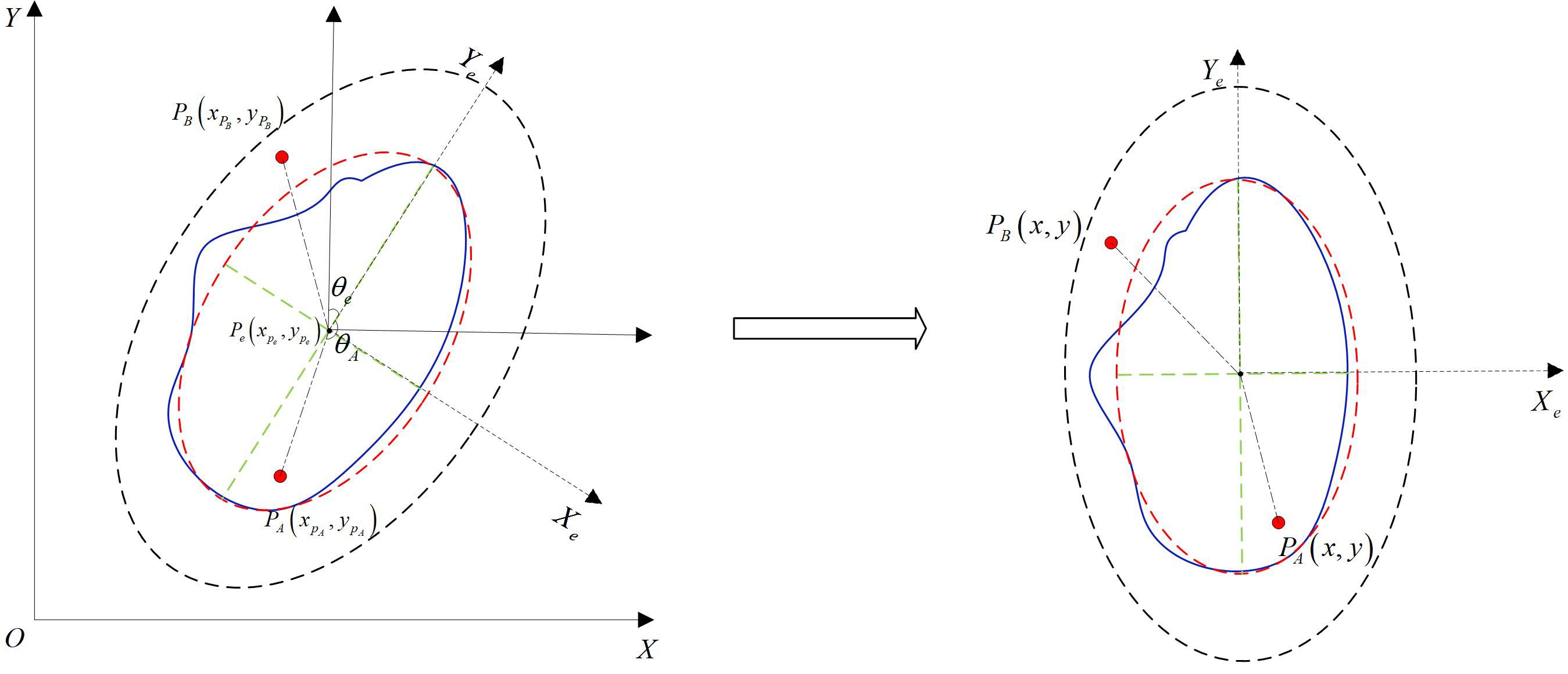
Figure 1. Schematic diagram of the coordinate transformation between Argo and the fitted eddy ellipse. $P_A$ and $P_B$ denotes the positional coordinates of the Argo float, and $P_e$ represents the coordinates of the eddy center.

2.5.2 Step 2

All Argo profiles captured by eddies were processed by calculating their sound speed profiles using temperature, salinity, and depth data. These profiles were then subjected to unsupervised clustering based on the characteristics of the study area. After classification, the coordinates of Argo floats within each category were projected onto the mean elliptical structure of eddies corresponding to that profile class.

2.5.3 Step 3

To better understand the thermal, saline, and sound speed structures of mesoscale eddies, it is necessary to subtract the monthly averaged climatological data at the corresponding latitude and longitude positions from the temperature and salinity profiles of the Argo floats, thereby obtaining the temperature and salinity anomalies of the profiles captured by the eddies.

2.5.4 Step 4

The Inverse Distance Weighting (IDW) method (Barnes, 1973) is used to perform weighted interpolation on the data. Additionally, for each depth layer, if any data point exceeds three times the upper quartile, it is considered an outlier and removed. The IDW interpolation uses a Gaussian weighting function to assign weights $W_i=e^{-{(d/R)}^2}$, within a 50 km radius around the eddy. As the distance increases, the weight of the Argo profiles decreases rapidly. The radius R is set to ensure that there are enough data points around each grid point while eliminating small-scale variability. After determining the weights, the values at the grid points are computed using the formula $V_{gp}={\displaystyle \sum W_i{V}_i/{\displaystyle \sum W_i}}$, where the $V_i$ represents the Argo value.

3 Result

3.1 Statistical characterization of elliptical mesoscale eddies

In order to understand the general characteristics of eddy shapes in the Philippine Sea, this paper presents a statistical analysis of the parameters of the best-fitting ellipses for the eddies in the region. Figure 2 shows the histogram of the eccentricities of the best-fitting ellipses, which indicates the degree of deviation of the Philippine Sea eddies from a circular shape. In the Philippine Sea, a small fraction of the eddies are circular (eccentricity of 0). The peak of the histogram is around 0.84–0.85, which is slightly higher compared to the eccentricities of elliptical eddies in global ocean regions reported in previous studies. The majority of the eddies have eccentricity values between 0.7 and 0.9, suggesting that most of the eddies in the Philippine Sea have an approximately elliptical structure. It is worth noting that a similar distribution of eccentricities has been observed for eddies in global oceans.

Figure 2

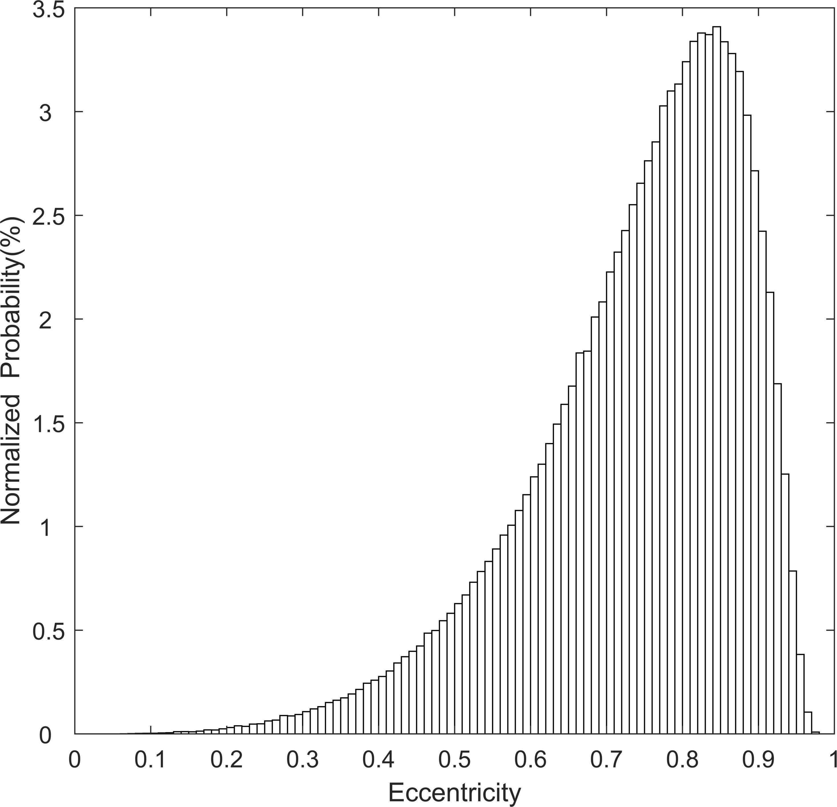
Figure 2. Normalized histogram of the eccentricity of the best-fit ellipses in an eddy-centric coordinate system for Philippine Sea eddies.

In addition, the authors also compiled data on the shape and orientation of the best-fit ellipses for eddies in the Philippine Sea. The semi-major axis (a) is 117.6 km, the semi-minor axis (b) is 73.7 km, the focal distance (c) is 91.6 km, and the eccentricity is 0.778. Compared to the average shape of global oceanic eddies reported by Chen et al. (2019) (a = 87.0 km, b = 54.0 km, e = 0.78), the eddies in the Philippine Sea have larger dimensions and focal distances, while the eccentricity is similar to that of global oceans. Additionally, we also obtained the rotation directions of the major axes for different types of eddies, with the specific results shown in Figure 3. The results in Figure 3 indicate a distinction in both the number and deflection direction between anticyclonic eddies (AE) and cyclonic eddies (CE). Cyclonic eddies are more numerous than anticyclonic eddies, and both types predominantly rotate in a northeast-southwest direction, with most angles concentrated around 80°/260°, which is consistent with findings from other regions in previous studies.

Figure 3

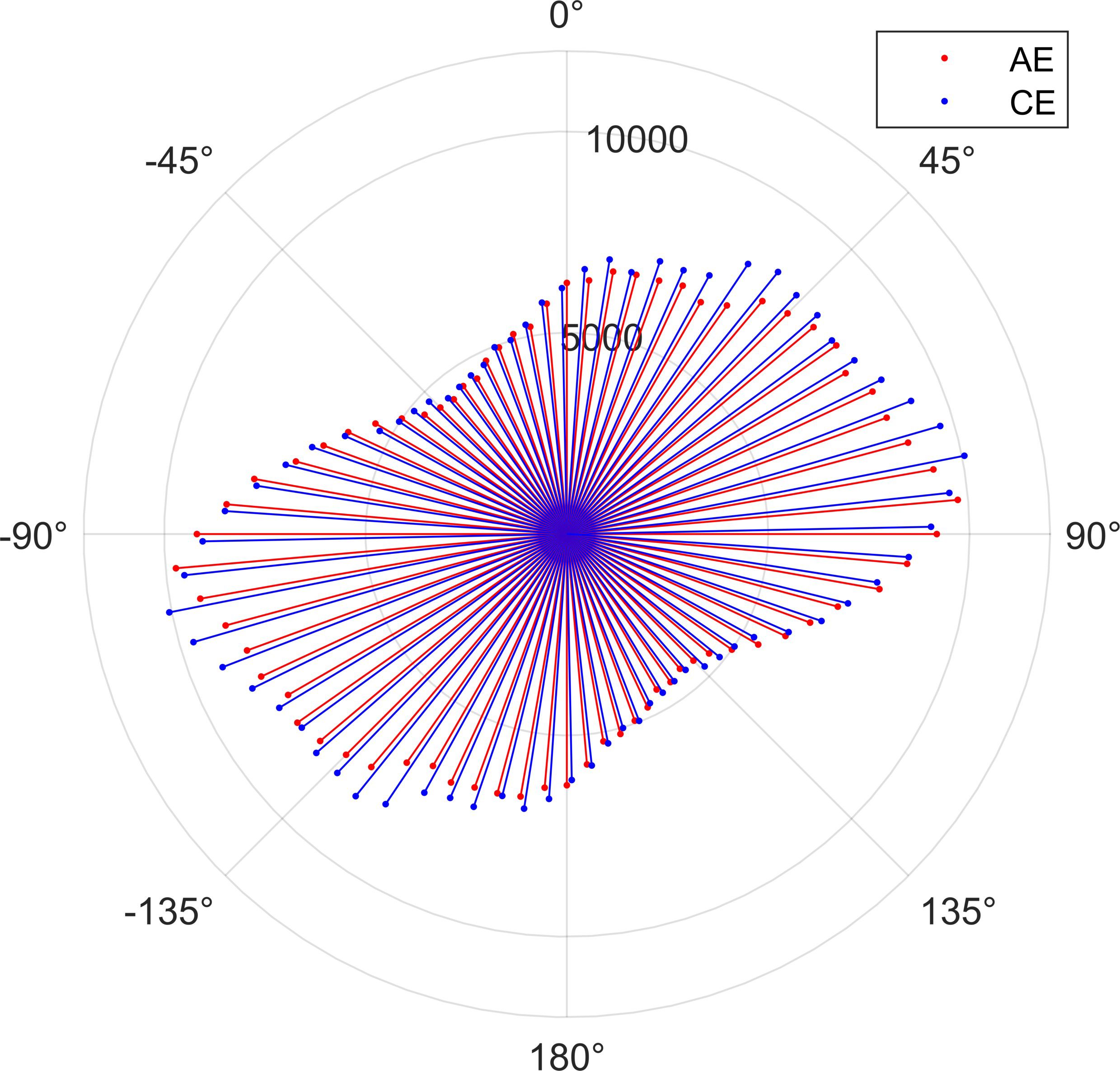
Figure 3. Histogram of the Rotation Direction of the Semi-Major Axis of the Best-Fit Ellipses for Mesoscale Eddies in the Philippine Sea.

The statistical results above indicate that more than 90% of the best-fit shapes of mesoscale eddies in the ocean are elliptical. This elliptical structure may lead to the formation of asymmetric features in the eddy, especially in the flow field structure. This structure can be compared to the Earth’s orbital path on a plane, where the flow speed is greater along the short axis and smaller along the long axis. Of course, these are just reasonable speculations. Whether the eddies truly exhibit this typical elliptical structure, and how the elliptical structure affects the temperature, salinity, and velocity fields of the eddy, will be discussed in the following sections.

3.2 Cluster analysis of Argo profiles captured by mesoscale eddies

Recent studies have shown that there are significant differences in the acoustic velocity anomalies of eddies in different ocean regions (Chen et al., 2022). Due to the unique geographical location of the Philippine Sea and the complexity of its wind and current systems, multiple sound speed profile structures may exist within the same sea area. This could lead to variations in the structure of mesoscale eddies. Exploring these differences and their potential impact on the formation of mesoscale eddies and their influence on oceanic parameters may be of significant importance. Therefore, it is necessary to distinguish the composite structures of eddies within the Philippine Sea.

With the advent of various clustering algorithms and the accumulation of oceanic Argo data, the traditional methods of defining oceanic structures based on existing frameworks and water masses of interest have gradually lost their predominance. Thanks to the spatial and temporal unbiased nature and the vast amount of Argo data, data-driven methods can significantly enhance the real-time identification of oceanic structures. The PCM clustering algorithm can accurately determine the number of clusters based on the Bayesian criterion, thereby identifying the types of composite eddies. Therefore, in this study, the PCM unsupervised clustering method was used to analyze the sound speed profile structures in the Philippine Sea, and different classification results were compared.

Figure 4 shows the clustering results of all Argo profile data captured by eddies, using the PCM profile clustering algorithm described in Section 2.4. The unsupervised clustering method requires the pre-determination of a K value. The PCM method uses the BIC approach to determine the optimal K value, which involves traversing different K values to find the one that minimizes the BIC. The calculations indicate that the Bayesian Information Criterion (BIC) reaches its minimum value when K=7, and the BIC value obtained for K=5 is close to that of K=7. However, upon comparing the actual conditions of the eddy structures with the clustering results of the sound speed profiles, it becomes evident that setting K=5 is more appropriate for the clustering analysis. This choice significantly reduces the likelihood of Argo profiles with similar characteristics being clustered into different profile types within the same eddy. Therefore, a K value of 5 was chosen for the clustering process in this study. The primary rationale for adopting five categories stems from the vast latitudinal span of the Philippine Sea, encompassing both tropical and subtropical zones. Due to the relatively weak seasonal variability in tropical waters, these were classified as a distinct category. Meanwhile, the northern subtropical region exhibits pronounced seasonal cycles and was accordingly subdivided into four categories. This classification scheme has been subsequently validated through our composite mesoscale eddy structures.

Figure 4

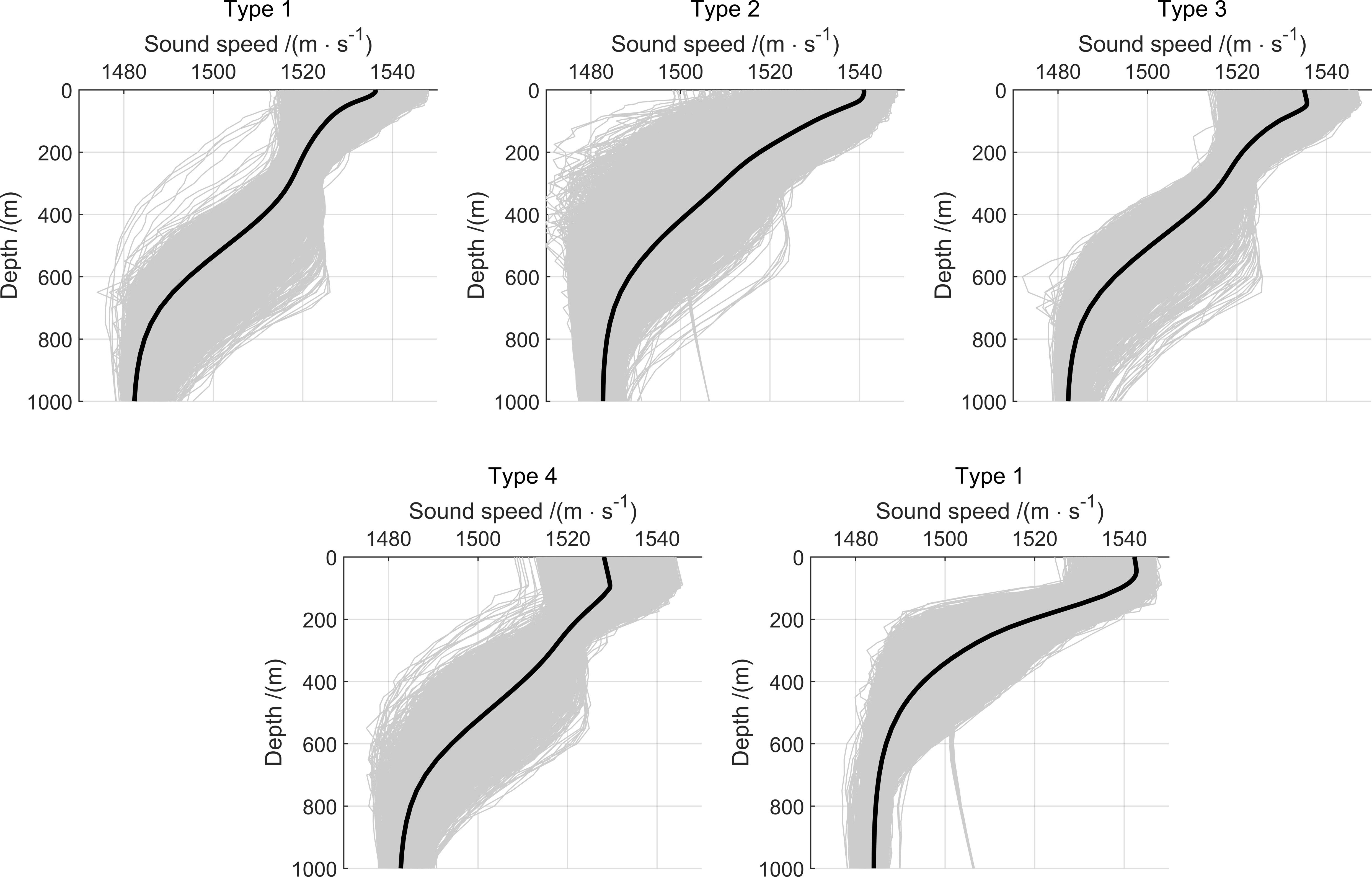
Figure 4. Clustering Results of Sound Speed Profiles in the Philippine Sea. The black solid line represents the average sound speed profile, and the gray dashed line represents the measured Argo sound speed profile.

Notably, the Argo profiles corresponding to each cluster demonstrate distinct regional and seasonal distribution characteristics, as evidenced by their spatial positions and monthly occurrence statistics presented in Figures 5, 6, respectively.

Figure 5

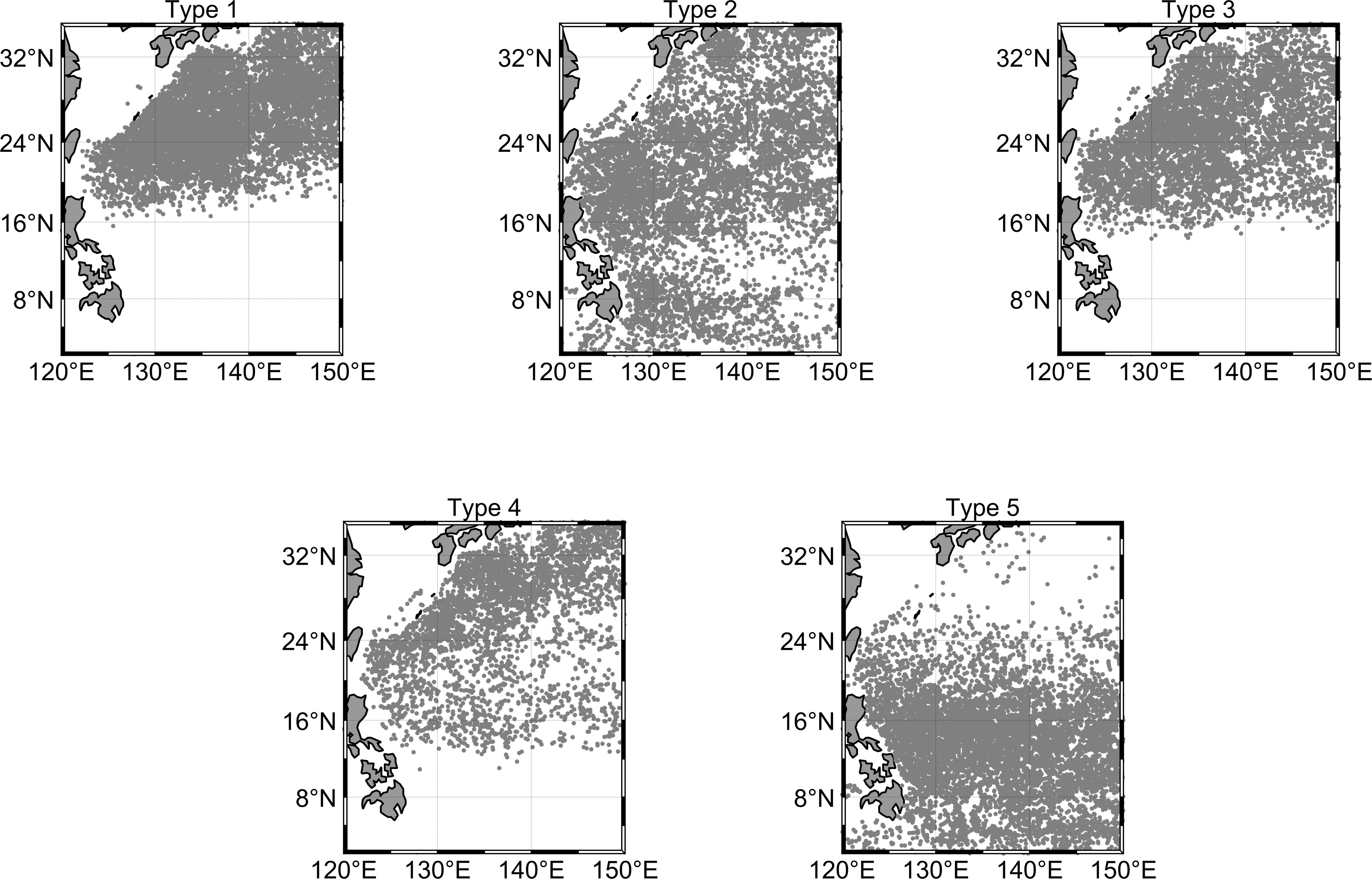
Figure 5. Distribution of Argo Locations for Clustering Results. Displayed are the positional coordinates of the Argo floats after clustering, as determined by the PCM profile clustering model.

Figure 6

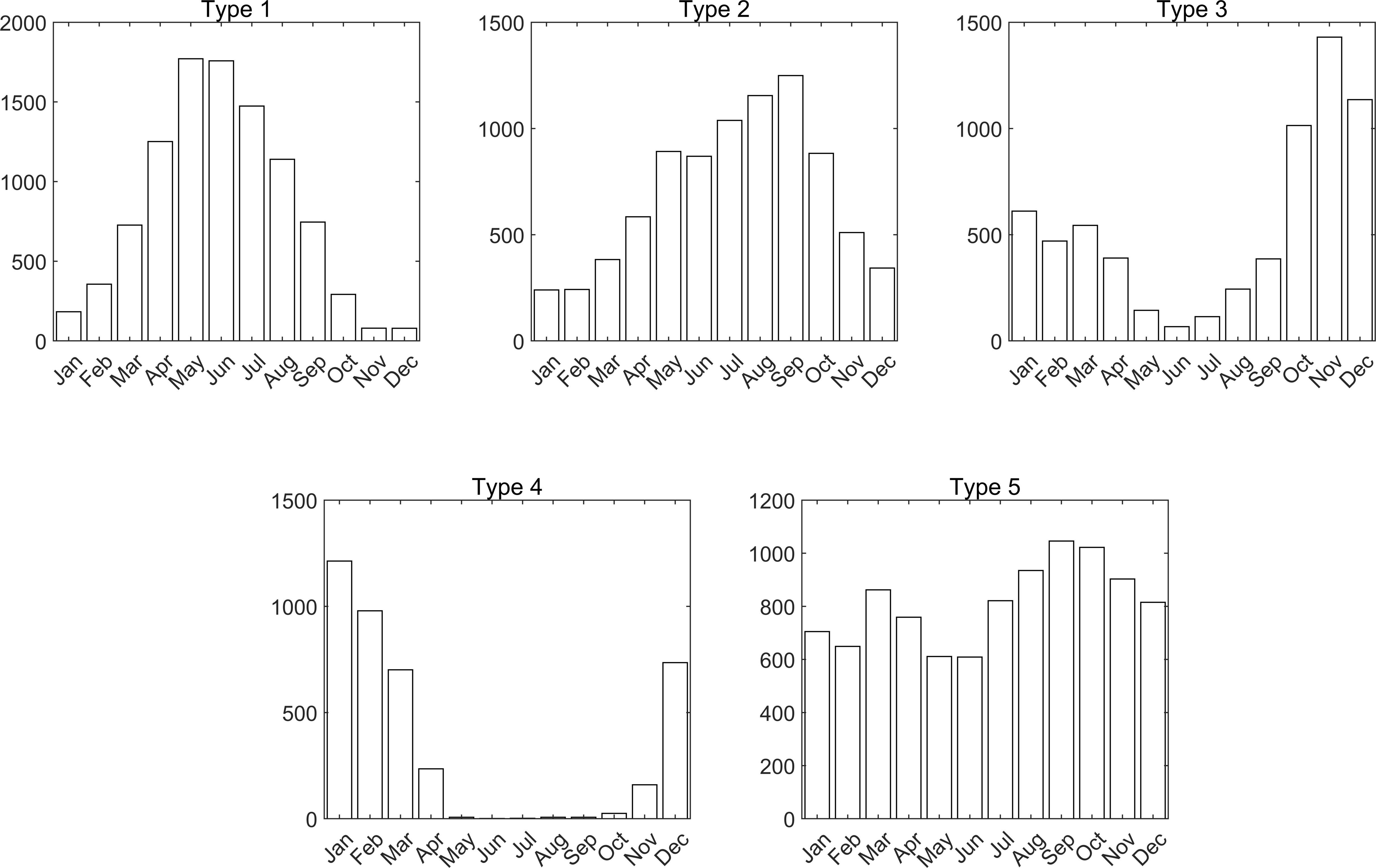
Figure 6. Seasonal Distribution of Argo for Clustering Results. The time statistics of the Argo floats corresponding to the five Argo location maps in Figure 5. The time statistics of the Argo floats corresponding to the five Argo location maps in Figure 5.

The Argo profiles clustered into five types are named as Types 1 to 5.

3.2.1 Type 1

The Argo profiles in this type are mainly concentrated from late spring to early summer, with a distribution range primarily in the waters north of 16°N. Based on the sound speed profile characteristics in Figure 4, it can be inferred that with the increasing solar radiation and the influence of modal water, the seasonal thermocline strengthens, and the seasonal thermocline separates from the main thermocline, forming a double-layer structure.

3.2.2 Type 2

The Argo profiles in this type are primarily concentrated from late summer to early autumn. Due to the relatively similar water mass structure in the Philippine Sea during the summer, this type has a broader distribution, covering most of the sea area. The main thermocline structure is thick and deep, with an average depth between 100-500m. Since the influence of modal water is minimal, a double-layer structure is not formed.

3.2.3 Type 3

The Argo profiles in this type are primarily concentrated from late autumn to early winter, with their distribution mainly in the waters north of 16°N. The structure of their sound speed profiles suggests that the eddy regions of this type are influenced by mode water, resulting in profiles that also display a double-thermocline structure. Furthermore, due to the reduction in wind mixing and solar radiation, the mixed layer in this type of profile is more pronounced, and the seasonal thermocline is weaker relative to that in summer.

3.2.4 Type 4

The profiles of this type are primarily concentrated in winter, with a distribution in the waters north of 12°N. During winter, with the weakest solar radiation, the surface sound speed is minimal, and the upper mixed layer is the thickest. The upper mixed layer shows a distinct positive sound speed gradient.

3.2.5 Type 5

This type is mainly distributed south of 24°N in the Philippine Sea. Due to the tropical nature of the region, this type of sound speed profile does not show a clear seasonal pattern and is more evenly distributed throughout the year. The region has a single-layer structure, with the average depth of the main thermocline being less than 300m. Due to stronger wind mixing, the sound speed profile is characterized by a relatively thick upper mixed layer.

3.3 Sectional structure of the composite eddy based on the elliptical model

A composite analysis of the eddy structure in the Philippine Sea was conducted based on the five types of Argo profile data obtained from clustering. To ensure the differentiation of composite mesoscale eddies under different background types and the accuracy of composites for the same type of mesoscale eddies, only Argo profiles from months with a quantity greater than 500 are selected for the composite analysis of each profile category. Using the eddy composite analysis method proposed in Section 2.5, we obtained the temperature composite structure of elliptical eddies in different sea areas of the Philippine Sea, classified based on the profile clustering results, as shown in Figure 7.

Figure 7

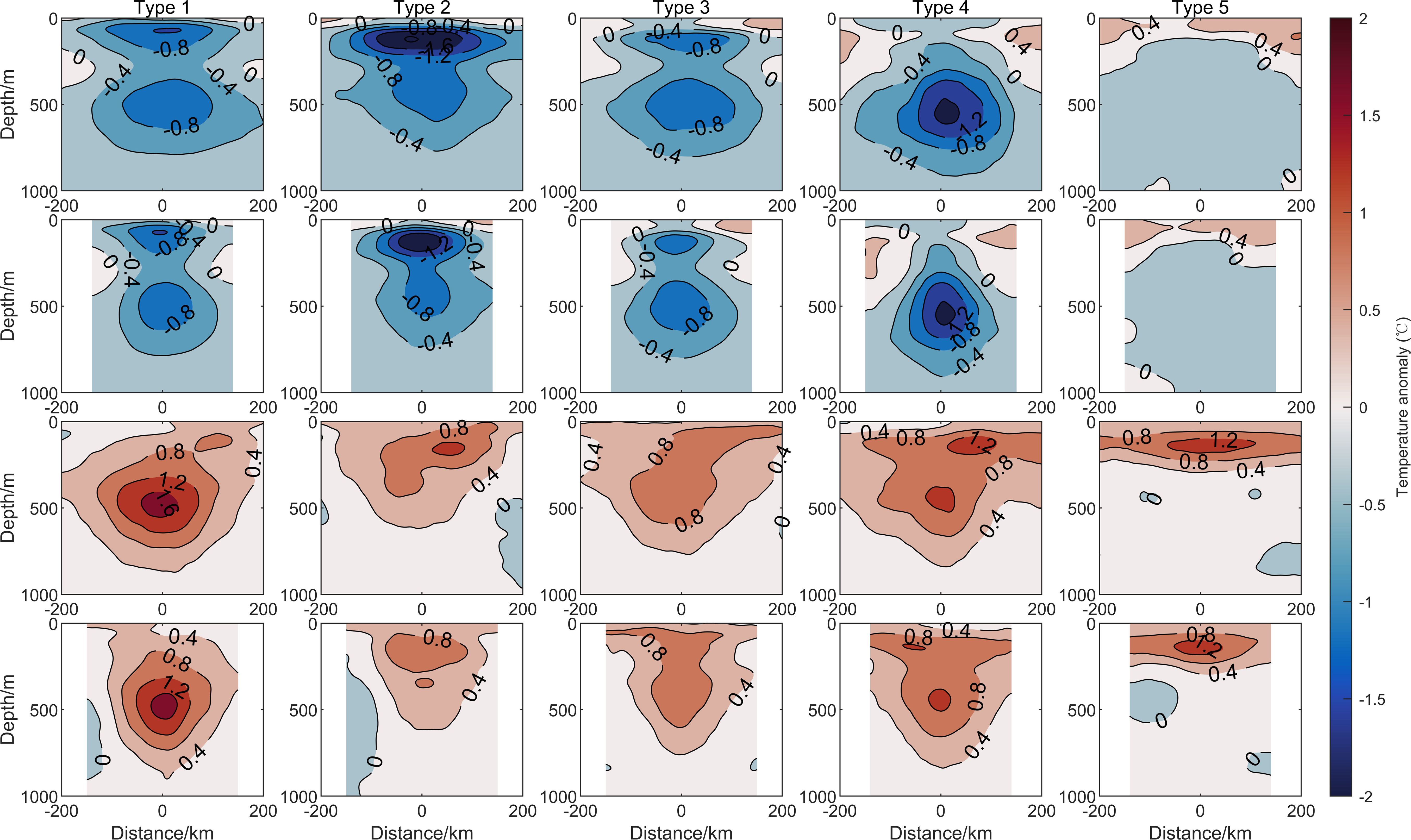
Figure 7. Schematic diagram of the temperature anomaly structure of the 5 types of composite mesoscale eddies. The first row shows the sectional views along the long axis of the cyclonic eddies for the five types, the second row shows the sectional views along the short axis of the cyclonic eddies for the five types, the third row shows the sectional views along the long axis of the anticyclonic eddies for the five types, and the fourth row shows the sectional views along the short axis of the anticyclonic eddies for the five types.

The reconstructed mesoscale eddy structures show significant differences in the mesoscale eddy anomaly structures obtained from different sound speed profile clustering results. This indicates that there are noticeable differences in the eddy structures of different water masses within the sea areas. Moreover, it is important to note that these differences are strongly correlated with the corresponding sound speed profile structures for each type of eddy.

The composite cyclonic eddy structures for Type 1 and Type 3 are similar, both displaying a distinct double-core structure. In Type 1, the upper eddy core is located in the 100–200 m depth range, while the lower eddy core is in the 300–600 m depth range, with both cores being of similar size. In Type 3, the upper eddy core is located deeper, in the 150–250 m range, compared to Type 1. This is because Type 3 primarily occurs in autumn, when the mixed layer is thicker, causing the thermocline to sink, and consequently, the eddy anomaly core also sinks. Unlike cyclonic eddies, the anticyclonic eddy structures exhibit certain seasonal differences. Due to the stronger permanent thermocline in spring, the temperature anomaly core of Type 1’s anticyclonic eddy is deeper and stronger, with the eddy core around 500 m depth and the temperature anomaly exceeding 1.6°C. In contrast, Type 3, which forms mainly in autumn, has a shallower temperature anomaly core with a weaker intensity.

The composite eddy structures of Type 2 mainly occur in summer. The cyclonic eddy anomaly structure is the strongest, with a temperature anomaly of up to -2°C, and the eddy core is located in the 100–250 m depth range. This is due to the weaker thermocline in summer compared to the tropical-type strong thermocline, allowing the eddy signal to penetrate into the thermocline structure. Additionally, compared to the sound speed profiles in spring and autumn, the thermocline in summer is stronger and less influenced by modal water, thus no distinct double-core eddy structure forms. The anticyclonic eddy has a weaker intensity, with a temperature anomaly around 1.2°C, and the eddy core is in the 100–250 m depth range, with a relatively shallow impact depth, reaching a maximum depth of about 600 m.

The composite eddy structure of Type 4 mainly occurs in winter. The key feature of its sound speed profile is the thickest upper mixed layer, which results in deeper eddy impacts compared to other types of cyclonic eddies. The eddy anomaly core is found in the 400–600 m depth range. In terms of intensity, the cyclonic eddy’s temperature anomaly structure in Type 4 is second only to Type 2, with a maximum temperature anomaly of about -1.6°C. The anticyclonic eddy, influenced by modal water, has two warm cores at around 150 m and 500 m depths.

The composite eddy structure of Type 5 is primarily concentrated in tropical seas. Due to the strongest and shallowest thermocline, the impact of the eddy is unable to penetrate the strong thermocline, causing the anticyclonic eddy core to be around 200 m deep, with a maximum temperature anomaly of about 1.2°C. The cyclonic eddy, compared to the anticyclonic eddy, has weaker intensity, and there is a positive temperature anomaly structure in the shallow surface layer, which may be related to the relatively uniform temperature in both the surface layer and below the thermocline in tropical seas. Since the tropical sea has relatively uniform temperature layers both above and below the main thermocline, the vertical displacement of water masses caused by eddy dynamics does not significantly affect the temperature anomaly structure. The eddy’s impact is relatively small, and the rising cold water from the cyclonic eddy is rapidly warmed in a short time, resulting in a less distinct cyclonic eddy structure.

For reference, we also present the cross-sectional structures of salinity and density anomalies induced by eddies, shown in Figures 8, 9, respectively. The salinity anomaly structure also exhibits a typical eddy structure. Under different acoustic profiling structures, the salinity anomaly structure influenced by eddies differs from the temperature anomaly structure. This is because the salinity profile exhibits a typical inverted “S” shape, and due to the different temperature profile structures in the region, it shows significant differences from the temperature anomaly structure.

Figure 8

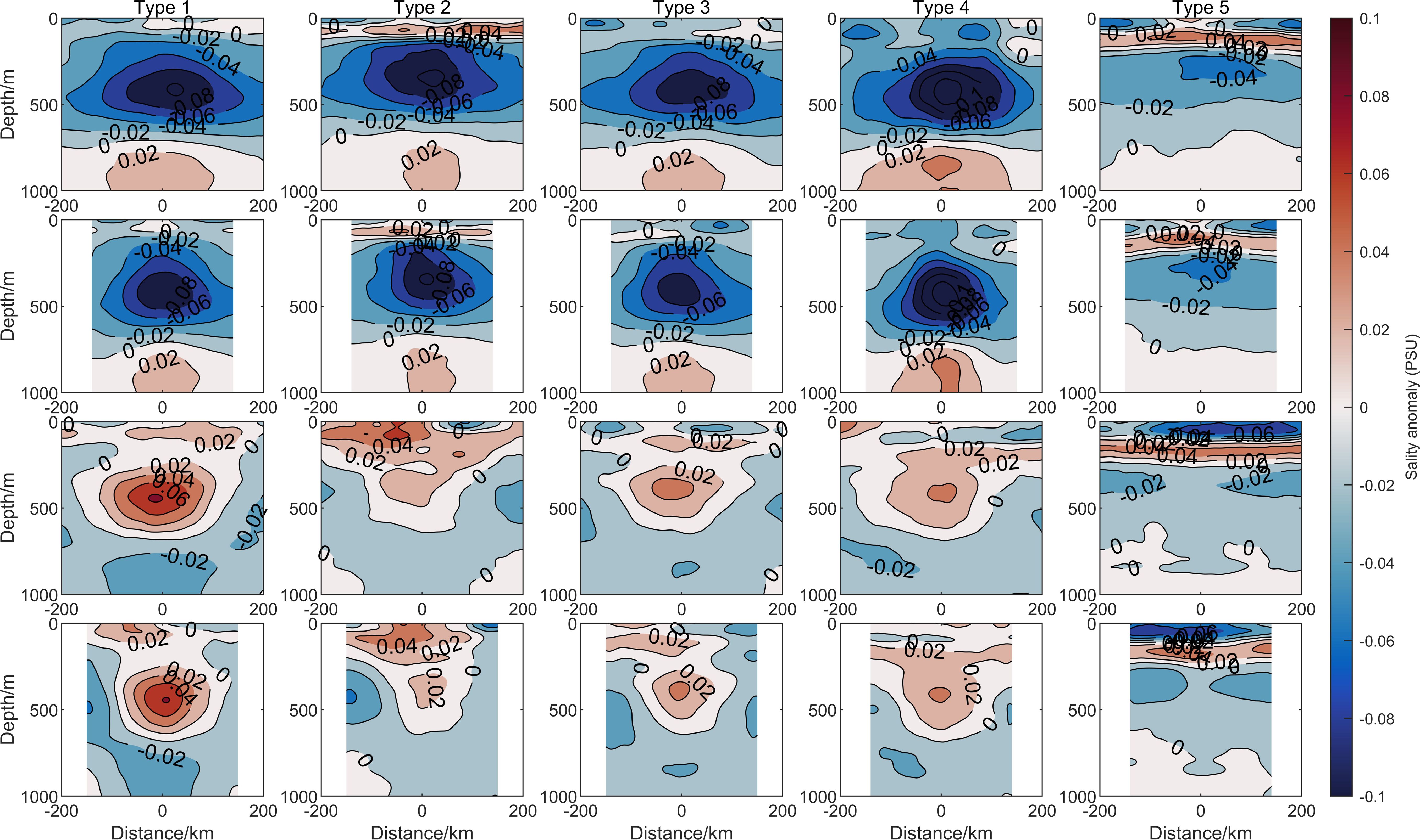
Figure 8. Schematic diagram of the salinity anomaly structure of the 5 types of composite mesoscale eddies. The subplots represent eddies that correspond to those in Figure 7.

Figure 9

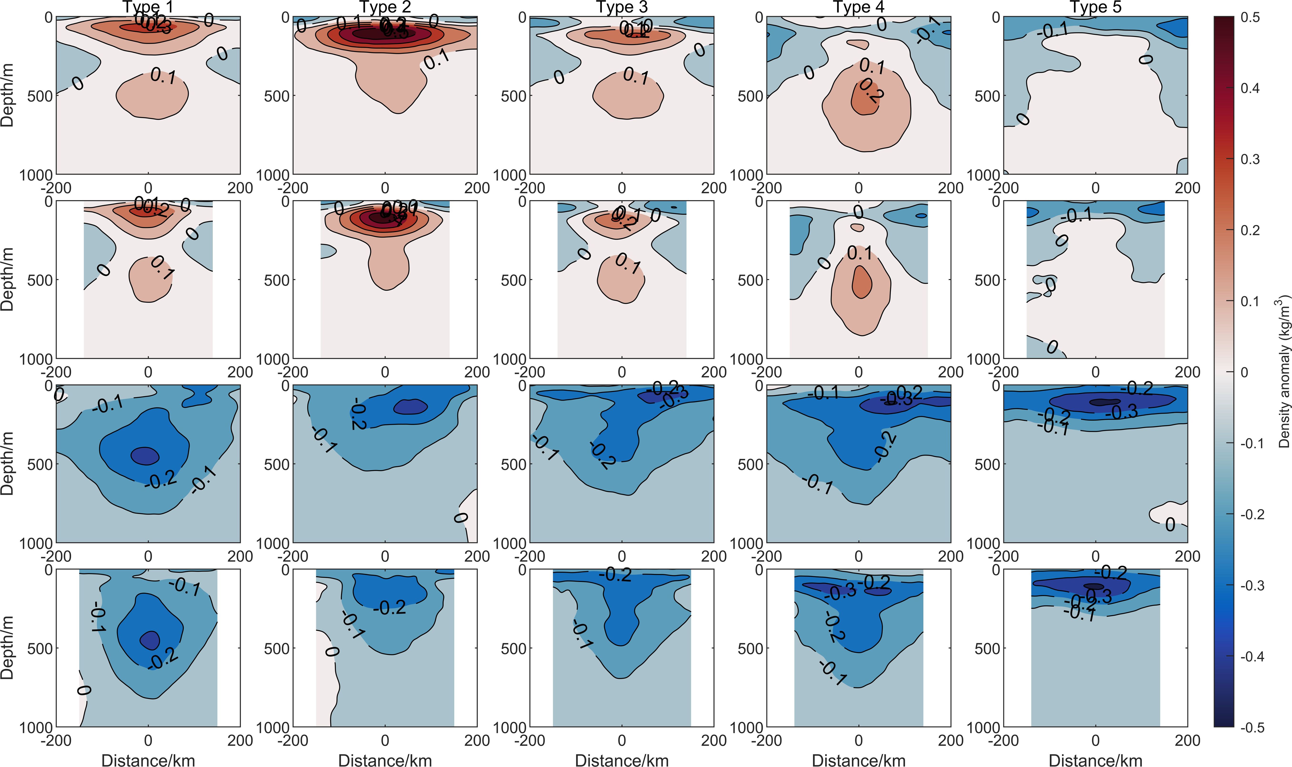
Figure 9. Schematic diagram of the density anomaly structure of the 5 types of composite mesoscale eddies. The subplots represent eddies that correspond to those in Figure 7.

Except for Type 5, the salinity anomaly structures of the other four types of cyclonic eddies are generally similar, with the maximum salinity anomaly depth ranging from 400 to 600 meters. However, there are some differences at the sea surface and at 1000 meters depth. In Type 1, there is a region of zero salinity anomaly at the sea surface. In Type 2, a positive salinity anomaly structure is found at 100 meters depth, overall presenting a “high-low-high” sandwich structure. Type 3 is similar to Type 1, with a zero salinity anomaly region at the sea surface, but it is offset from the eddy center. Type 4 has a strong negative salinity anomaly core at the sea surface, which may be related to the seasonal surface current and precipitation characteristics, and its specific causes and development require further investigation. In contrast to the first four types of cyclonic eddies, Type 5 exhibits a salinity anomaly structure that presents a “low-high-low” pattern from the sea surface to 500 meters depth. The low salinity anomaly is more pronounced below the eddy’s pycnocline, and the anticyclonic eddy exhibits a more obvious low salinity anomaly at the sea surface. The specific reasons for this structure require further discussion in future studies.

The density anomaly structure generally exhibits characteristics opposite to those of the temperature anomaly structure, where the temperature anomaly is higher, the density anomaly is lower, and where the temperature anomaly is lower, the density anomaly is higher. The influence of salinity is weak in this context. This can be estimated using the seawater equation of state, which shows that the contribution of temperature anomalies to density anomalies within the eddies is about 90%. Similar to the distribution of temperature anomalies, the density anomaly structure also demonstrates clear seasonal and regional characteristics, although the magnitude of the density anomaly is smaller than that of the temperature anomaly, with the maximum density anomaly ranging within -0.5 to 0.5 kg/m³.

From the cross-sectional diagrams of the temperature, salinity, and density anomaly structures of the eddies, it can be observed that the composite analysis method of elliptical eddies leads to some differences between the long axis and short axis of the eddy. First, in terms of the influence range, the influence range of the long axis direction of the composite eddy is about 50% larger than that of the short axis direction. This result aligns more closely with the actual mesoscale eddy structures in the ocean. According to the geostrophic flow calculation method, the elliptical structure of the mesoscale eddy may lead to an increase in flow velocity in the short axis direction within the eddy.

In terms of eddy intensity, the differences in temperature, salinity, and density anomalies from inside to outside the eddy along the long axis and short axis directions are consistent. However, due to the larger influence range along the long axis, its gradient is smaller. This causes a change in the gradient of sound velocity in the horizontal direction, which may, in turn, affect sound propagation characteristics. Furthermore, the anomaly structures along the long axis and short axis directions of the eddy are not completely identical, indicating that the eddies in the actual ocean exhibit anisotropy. Their true characteristics require further investigation in subsequent studies.

4 Discussion

4.1 Traditional eddy composite analysis method

The traditional eddy composite analysis generally requires Argo or CTD profile data within 1.5 times the radius of the eddy. The distance from the profile location to the eddy center is normalized using the radius r, where a normalized distance of 0 corresponds to the eddy center, and a normalized distance of 1 corresponds to the contour line defining the eddy (Sandalyuk et al., 2020).his method is based on the assumption made by Zhang et al (Zhang et al., 2013), which suggests that mesoscale eddies, regardless of their amplitude, polarity, or scale, have the same structure. The data profile projection method in the composite approach is shown in Figure 10.

Figure 10

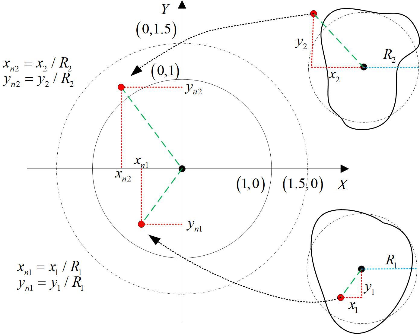
Figure 10. Schematic of the Argo coordinate system in the traditional eddy composite method. the red dots denote the positions of the Argo floats, the irregular black solid lines delineate the eddy boundaries, the small dashed circle on the right represents the fitted circular boundary, and the larger diagram on the left illustrates the relative positions of the eddies and Argo floats after projection.

The radial distribution of temperature and salinity anomalies reconstructed based on the above method can be considered to have universality. Subsequent work following this technique has indeed confirmed the feasibility of this method (He et al., 2018). In order to compare with the eddy composite method proposed in this paper, the authors applied this method to composite the eddy structure in the Philippine Sea, and the reconstruction results will be detailed in Section 4.2.

4.2 Comparison of the results from two eddy composite analysis methods

The conventional eddy composite results are shown in Figure 11. Compared with the method proposed in this study based on sound speed profile clustering and elliptical eddy composition, the traditional eddy composite method yields results with more universal structural characteristics. However, these results exhibit certain discrepancies from the diverse elliptical structures of mesoscale eddies observed in actual oceanic conditions. The temperature, salinity, and density anomaly structures of the mesoscale eddies in terms of depth and intensity, as obtained by the traditional composite method, show that the temperature and salinity anomaly structures of cyclonic eddies are more similar to Type 1 and Type 3 structures introduced in Section 3.3. On the other hand, the temperature and salinity anomaly core of anticyclonic eddies, influenced by the tropical anticyclonic eddy from Type 5, leads to an upward shift of the eddy core, with an impact range similar to Type 2 described in Section 3.3. The density anomaly core still shows a negative correlation with the temperature anomaly core. In terms of intensity, the mesoscale eddies obtained by the traditional method result in an over-averaged eddy strength due to the neglect of the enhancement of temperature and salinity gradients caused by the velocity increase in the short-axis direction of the elliptical eddy structure, as well as the differences in eddy strength across different regions or seasons of the same sea area. This over-averaging makes it difficult to accurately represent the eddy structures within the sea area.

Figure 11

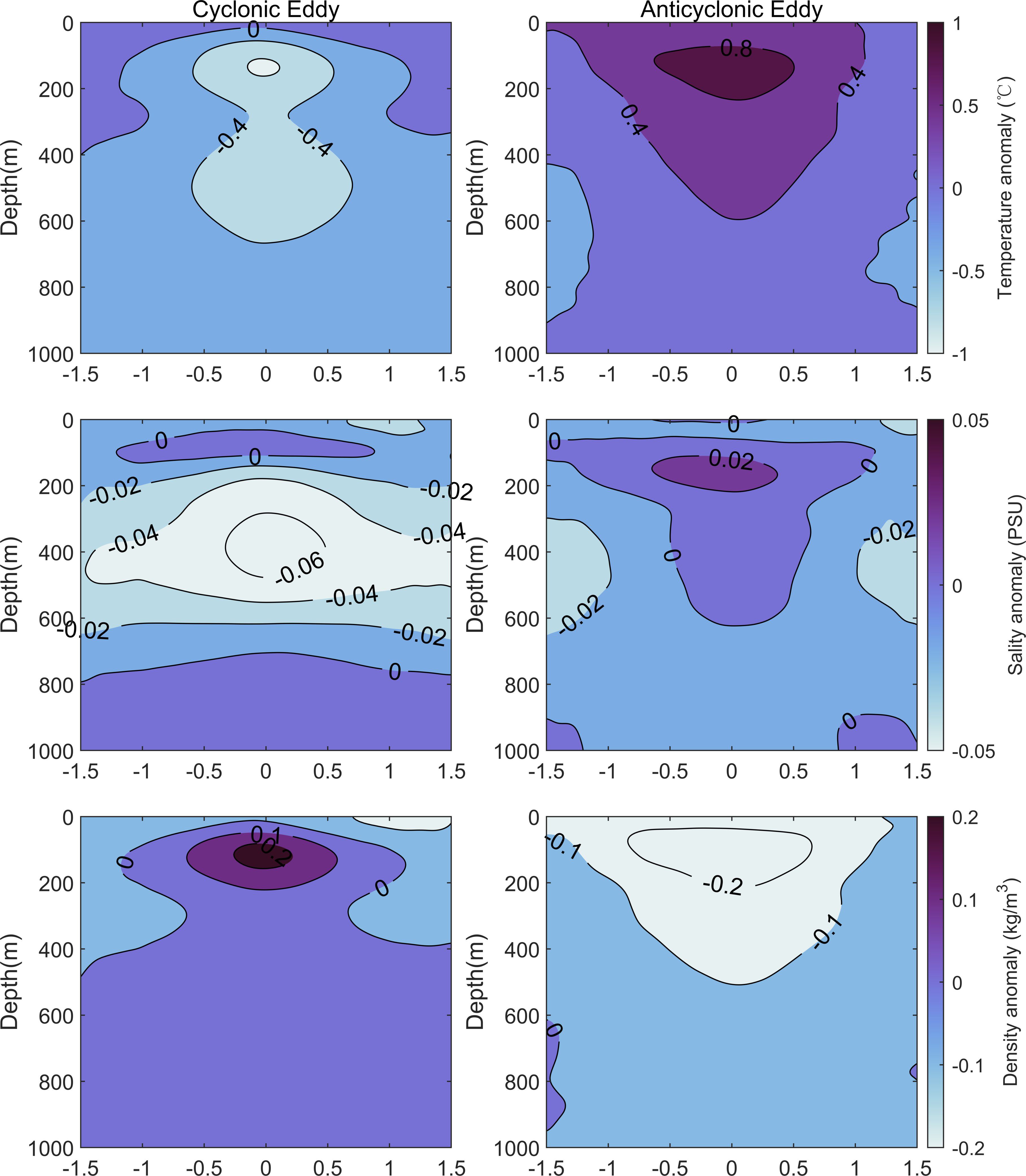
Figure 11. Schematic of the mesoscale eddy structure in the Philippine Sea obtained using the traditional composite analysis method. The left column presents data for cyclonic eddies, while the right column displays data for anticyclonic eddies. From top to bottom, the figures depict the cross-sectional profiles of temperature, salinity, and density of composite mesoscale eddies, respectively.

To further validate the accuracy of the eddy structure obtained by the method proposed in this paper, the eddy recognition method was used to extract several typical vertical structures of eddies in the Philippine Sea from the model data. Taking the anticyclonic eddy as an example, four typical vertical temperature sections of anticyclonic eddies are shown in Figure 12.

Figure 12

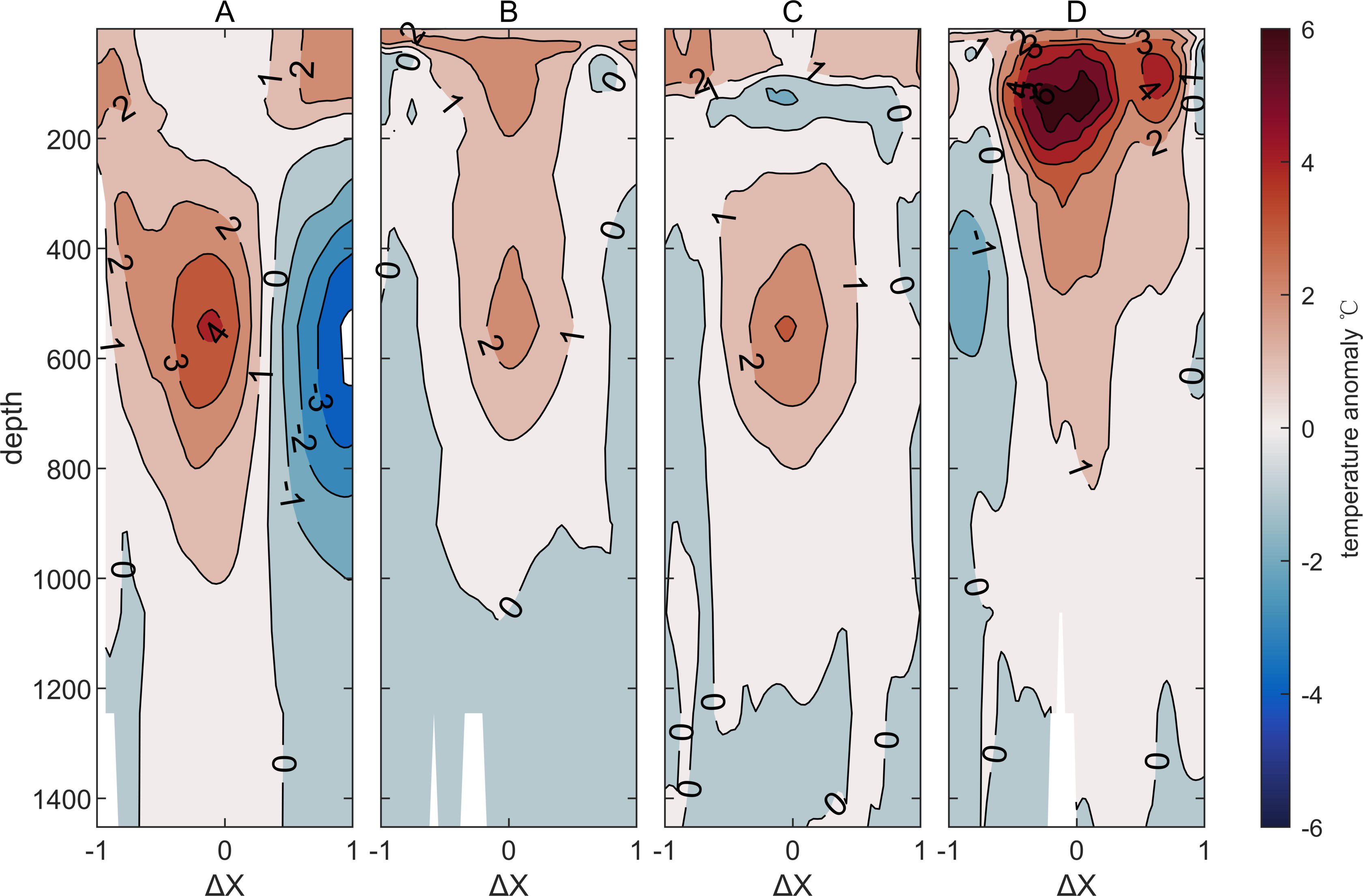
Figure 12. Temperature vertical profiles of anticyclonic eddies in the Philippine Sea obtained from model data (Global Ocean Physics Reanalysis Data). Subfigures (A-D) correspond respectively to Type 1, Type 3, and Type 5 anticyclonic eddy structures within the composite eddy framework discussed in this paper.

Comparing Figures 7, 12, it can be seen that in terms of the depth of eddy influence, the composite eddy method proposed in this paper provides a better description of the eddies. Compared to the traditional method, it more accurately reflects the depth of temperature anomaly influence of eddies across different regions and seasons. However, in terms of intensity, due to certain errors in the simulation of eddy intensity in the model data and the possible weakening effect of the eddy composite analysis method on eddy strength, corrections for eddy intensity can be made in subsequent applications based on a small number of observed profiles.

Despite this, the composite method proposed in this paper represents significant progress over the traditional method. First, in terms of eddy intensity, the method separates eddies of different intensities based on profile classification, which reduces the weakening effect of the composite method on eddy intensity. In terms of eddy influence depth, the method proposed here more accurately composites the influence depth of different types of eddies compared to traditional methods, making it more accurate for predicting the impact of eddies. Regarding the asymmetric structure of eddies, the composite method presented here is based on the characteristics of eddies in the Philippine Sea, using the best-fit elliptical structure for composite analysis. This highlights the impact of the elliptical flow field structure on the temperature and salinity anomaly structures of eddies and emphasizes the different influence ranges of the long and short axes of the best-fit elliptical structure, which is of practical significance for real-world applications.

5 Summary and conclusion

This study proposes a new composite analysis method based on sound velocity profile clustering and the best-fit elliptical model for eddies. This method takes into account that within the same oceanic region, the intensity and depth of eddy influence can be affected by the water mass structure and the shape of the eddies, leading to different characteristics. Therefore, using the PCM profile clustering algorithm and the elliptical eddy composite method, this paper analyzes the temperature, salinity, and density anomaly structures of active mesoscale eddies in the Philippine Sea under five typical sound velocity profiles, using a large amount of Argo profile data and the META3.2 product from 2007 to 2022.

First, the surface structure of eddies in the Philippine Sea was investigated. Using the best-fit elliptical method, the directional characteristics of the major axes of mesoscale eddies in the region were statistically analyzed. It was found that cyclonic eddies are more numerous than anticyclonic eddies, and the major axes of the eddies are predominantly oriented along the northeast-southwest direction, with most of the angles concentrated around 80°/260°. Furthermore, the eccentricity of the ellipses in the region was also statistically analyzed. The distribution of eccentricities showed a skewed pattern with a peak between 0.84 and 0.85, confirming that the majority of mesoscale eddies in the ocean are elliptical in shape.

Next, the composite eddy’s structure exhibited significant regional dependence, which contrasts with the globally universal structure of pressure anomalies identified by Zhang et al (Zhang et al., 2013). The composite results of eddies in the Philippine Sea after profile clustering show clear regional and seasonal variations, providing valuable reference for future eddy structure predictions. Based on the clustering results, eddies in the region were classified into five types, each with its typical characteristics. This classification has strong guiding significance for targeted predictions of eddies at different times. According to the profile structure of each clustering result, the temperature and salinity anomalies of the eddies exhibited different regional characteristics. The area producing Type 5 eddies is mainly concentrated in the tropics. Due to the strong permanent stratification in tropical waters, the influence of the eddies is difficult to penetrate the stratified layer. As a result, the cyclonic eddies mainly affect the area below the thermocline, with weaker intensity, while the anticyclonic eddies primarily affect the region above the main thermocline at depths of 100–200 meters.

Types 1 and 3 of the Argo profiles are mainly concentrated in spring and autumn. The composite eddy structures of these two types are similar, with both cyclonic eddies showing a double-core structure. In Type 1, the upper eddy core is located at depths of 100–200 meters, and the lower core is located at depths of 300–600 meters, with the two cores nearly connected. In comparison, the upper core of Type 3 is deeper, located at depths of 150–250 meters, which is related to the thicker mixed layer in autumn. Similar to cyclonic eddies, the anticyclonic eddy structures of these two types are also similar, but the double warm-core structure does not appear. Additionally, due to the strong permanent stratification in spring, the core of the anticyclonic eddy is deeper, located between 400–600 meters, with temperature anomalies greater than 1.6°C. Type 2 Argo profiles are mainly concentrated in summer, when the stratification is weaker, allowing the eddy signal to penetrate the stratified structure. As the eddies absorb more energy in summer, cyclonic eddy intensity is the strongest, with temperature anomaly structures reaching -2°C, and the eddy core located at depths of 100–500 meters. The anticyclonic eddy intensity is weaker, with temperature anomalies around 1.2°C, and the eddy core is located at depths of 200–400 meters, with a maximum influence depth of about 700 meters. In winter, the eddy core is deeper, with cyclonic eddy cores at depths of 400–600 meters, and maximum temperature anomalies of approximately -1.6°C. Anticyclonic eddies exhibit two core structures at depths of 100 meters and 500 meters.

To verify the superiority of the proposed composite method, the traditional eddy composite method was applied to the same data. The temperature profile structures of several typical mesoscale eddies in the Philippine Sea, identified from model data, were compared. The results show that in terms of eddy intensity, the proposed method produces stronger eddies, which are closer to the eddies simulated by the model data. In terms of influence depth, the method proposed in this paper can better reflect the different types of eddy structures within the same oceanic region, while the traditional method only provides an overall average for the region. In terms of eddy models, the elliptical structure model proposed in this paper better fits the actual eddy characteristics of the region and highlights the differences in eddy structures along the long and short axes of the elliptical shape.

In conclusion, extensive in-situ eddy data show that both the surface and sub-surface structures of oceanic eddies are elliptical in shape. Additionally, the structures of eddies in different regions also exhibit variations. Therefore, the new composite and clustering approach adopted in this study has provided a three-dimensional structure for the Philippine Sea eddies based on the elliptical model, which is significant for global eddy characterization. Moreover, when studying the eddy flux of heat and substances in the ocean, the elliptical structure provides a more reasonable explanation compared to a circular structure.

Data availability statement

The original contributions presented in the study are included in the article/supplementary material. Further inquiries can be directed to the corresponding author.

Author contributions

XZ: Conceptualization, Data curation, Formal Analysis, Funding acquisition, Investigation, Methodology, Project administration, Resources, Software, Supervision, Validation, Visualization, Writing – original draft, Writing – review & editing. QL: Investigation, Methodology, Software, Writing – review & editing. XY: Conceptualization, Investigation, Methodology, Writing – review & editing. GZ: Conceptualization, Investigation, Methodology, Writing – review & editing. YM: Investigation, Methodology, Writing – review & editing.

Funding

The author(s) declare that no financial support was received for the research and/or publication of this article.

Acknowledgments

The mesoscale eddy trajectory atlas products from AVISO(https://www.aviso.altimetry.fr) were used. Argo profiles were collected from https://data-argo.ifremer.fr/ and WOA23 climatological atlas was downloaded from NOAA (https://www.ncei.noaa.gov/products/world-ocean-atlas).

Conflict of interest

The authors declare that the research was conducted in the absence of any commercial or financial relationships that could be construed as a potential conflict of interest.

Generative AI statement

The author(s) declare that no Generative AI was used in the creation of this manuscript.

Publisher’s note

All claims expressed in this article are solely those of the authors and do not necessarily represent those of their affiliated organizations, or those of the publisher, the editors and the reviewers. Any product that may be evaluated in this article, or claim that may be made by its manufacturer, is not guaranteed or endorsed by the publisher.

References

Akima H. (1970). A new method of interpolation and smooth curve fitting based on local procedures. J. ACM (JACM). 17, 589–602. doi: 10.1145/321607.321609

Crossref Full Text | Google Scholar

Barnes S. L. (1973). Mesoscale objective map analysis using weighted time-series observations. Series : NOAA technical memorandum ERL NSSL, 62. Available online at: https://repository.library.noaa.gov/view/noaa/17647.

Google Scholar

Chaigneau A., Le Texier M., Eldin G., Grados C., Pizarro O. (2011). Vertical structure of mesoscale eddies in the eastern South Pacific Ocean: A composite analysis from altimetry and Argo profiling floats. J. Geophys. Res.: Oceans. 116, C11025. doi: 10.1029/2011JC007134

Crossref Full Text | Google Scholar

Chelton D. B., Schlax M. G., Samelson R. M. (2011). Global observations of nonlinear mesoscale eddies. Prog. Oceanogr. 91, 167–216. doi: 10.1016/j.pocean.2011.01.002

Crossref Full Text | Google Scholar

Chen G., Han G., Yang X. (2019). On the intrinsic shape of oceanic eddies derived from satellite altimetry. Remote Sens. Environ. 228, 75–89. doi: 10.1016/j.rse.2019.04.011

Crossref Full Text | Google Scholar

Chen C. T., Millero F. J. (1977). Speed of sound in seawater at high pressures. J. Acoustical. Soc. America 62, 1129–1135. doi: 10.1121/1.381646

Crossref Full Text | Google Scholar

Chen W., Zhang Y., Liu Y., Ma L., Wang H., Ren K., et al. (2022). Parametric model for eddies-induced sound speed anomaly in five active mesoscale eddy regions. J. Geophys. Res.: Oceans. 127, e2022JC018408. doi: 10.1029/2022JC018408

Crossref Full Text | Google Scholar

Fofonoff N. P., Millard R. Jr (1983). Algorithms for the computation of fundamental properties of seawater. Paris, France, UNESCO, 53pp. (UNESCO Technical Papers in Marine Sciences; 44). doi: 10.25607/OBP-1450

Crossref Full Text | Google Scholar

Han G., Tian F., Ma C., Chen G. (2021). The geometry of mesoscale eddies in the South China Sea: characteristics and implications. Int. J. Digital. Earth 14, 464–479. doi: 10.1080/17538947.2020.1842523

Crossref Full Text | Google Scholar

He Y., Feng M., Xie J., He Q., Liu J., Xu J., et al. (2021). Revisit the vertical structure of the eddies and eddy-induced transport in the leeuwin current system. J. Geophys. Res.: Oceans. 126, e2020JC016556. doi: 10.1029/2020JC016556

Crossref Full Text | Google Scholar

He Q., Zhan H., Cai S., He Y., Huang G., Zhan W. (2018). A new assessment of mesoscale eddies in the south China sea: surface features, three-dimensional structures, and thermohaline transports. J. Geophys. Res.: Oceans. 123, 4906–4929. doi: 10.1029/2018JC014054

Crossref Full Text | Google Scholar

Hu D., Wu L., Cai W., Gupta A. S., Ganachaud A., Qiu B., et al. (2015). Pacific western boundary currents and their roles in climate. Nature 522, 299–308. doi: 10.1038/nature14504

PubMed Abstract | Crossref Full Text | Google Scholar

Itoh S., Yasuda I. (2010). Water mass structure of warm and cold anticyclonic eddies in the western boundary region of the subarctic North Pacific. J. Phys. Oceanogr. 40, 2624–2642. doi: 10.1175/2010JPO4475.1

Crossref Full Text | Google Scholar

Li L., Nowlin W. D., Jilan S. (1998). Anticyclonic rings from the kuroshio in the south China sea. Deep. Sea. Res. Part I.: Oceanogr. Res. Papers. 45, 1469–1482. doi: 10.1016/s0967-0637(98)00026-0

Crossref Full Text | Google Scholar

Li H., Xu F., Wang G. (2022). Global mapping of mesoscale eddy vertical tilt. J. Geophys. Res.: Oceans. 127, e2022JC019131. doi: 10.1029/2022JC019131

Crossref Full Text | Google Scholar

Lin X., Dong C., Chen D., Liu Y., Yang J., Zou B., et al. (2015). Three-dimensional properties of mesoscale eddies in the South China Sea based on eddy-resolving model output. Deep. Sea. Res. Part I.: Oceanogr. Res. Papers. 99, 46–64. doi: 10.1016/j.dsr.2015.01.007

Crossref Full Text | Google Scholar

Locarnini R. A., Mishonov A. V., Baranova O. K., Reagan J. R., Boyer T. P., Seidov D., et al. (2024). World Ocean Atlas 2023, Volume 1: Temperature. Mishonov A., Technical Editor. NOAA Atlas NESDIS 89, 52 pp. doi: 10.25923/54bh-1613

Crossref Full Text | Google Scholar

Ma Y., Li Q., Wang H., Yu X., Li S. (2024). Composite vertical structures and spatiotemporal characteristics of abnormal eddies in the Japan/East Sea: a synergistic investigation using satellite altimetry and Argo profiles. Front. Marine. Sci. 10. doi: 10.3389/fmars.2023.1309513

Crossref Full Text | Google Scholar

Mackenzie K. V. (1981). Nine-term equation for sound speed in the oceans. J. Acoustical. Soc. America 70, 807–812. doi: 10.1121/1.386920

Crossref Full Text | Google Scholar

Mason E., Pascual A., Mcwilliams J. C. (2014). A new sea surface height–based code for oceanic mesoscale eddy tracking. J. Atmospheric. Oceanic. Technol. 31, 1181–1188. doi: 10.1175/JTECH-D-14-00019.1

Crossref Full Text | Google Scholar

Maze G., Mercier H., Fablet R., Tandeo P., Lopez Radcenco M., Lenca P., et al. (2017). Coherent heat patterns revealed by unsupervised classification of Argo temperature profiles in the North Atlantic Ocean. Prog. Oceanogr. 151, 275–292. doi: 10.1016/j.pocean.2016.12.008

Crossref Full Text | Google Scholar

Pegliasco C., Chaigneau A., Morrow R. (2015). Main eddy vertical structures observed in the four major Eastern Boundary Upwelling Systems. J. Geophys. Res.: Oceans. 120, 6008–6033. doi: 10.1002/2015JC010950

Crossref Full Text | Google Scholar

Pegliasco C., Delepoulle A., Mason E., Morrow R., Faugère Y., Dibarboure G. (2022). META3.1exp: a new global mesoscale eddy trajectory atlas derived from altimetry. Earth Syst. Sci. Data 14, 1087–1107. doi: 10.5194/essd-14-1087-2022

Crossref Full Text | Google Scholar

Qiu B. (1999). Seasonal eddy field modulation of the north pacific subtropical countercurrent: TOPEX/poseidon observations and theory. J. Phys. Oceanogr. 29, 2471–2486. doi: 10.1175/1520-0485(1999)029<2471:SEFMOT>2.0.CO;2

Crossref Full Text | Google Scholar

Qiu B., Chen S. (2010). Interannual variability of the north pacific subtropical countercurrent and its associated mesoscale eddy field. J. Phys. Oceanogr. 40, 213–225. doi: 10.1175/2009JPO4285.1

Crossref Full Text | Google Scholar

Qiu C., Mao H., Liu H., Xie Q., Yu J., Su D., et al. (2019). Deformation of a warm eddy in the northern South China sea. J. Geophys. Res.: Oceans. 124, 5551–5564. doi: 10.1029/2019JC015288

Crossref Full Text | Google Scholar

Qiu C., Yi Z., Su D., Wu Z., Liu H., Lin P., et al. (2022). Cross-slope heat and salt transport induced by slope intrusion eddy’s horizontal asymmetry in the Northern South China sea. J. Geophys. Res.: Oceans. 127, e2022JC018406. doi: 10.1029/2022JC018406

Crossref Full Text | Google Scholar

Roemmich D., Gilson J. (2001). Eddy transport of heat and thermocline waters in the North Pacific: A key to interannual/decadal climate variability? J. Phys. Oceanogr. 31, 675–687. doi: 10.1175/1520-0485(2001)031<0675:ETOHAT>2.0.CO;2

Crossref Full Text | Google Scholar

Sandalyuk N. V., Bosse A., Belonenko T. V. (2020). The 3-D structure of mesoscale eddies in the lofoten basin of the norwegian sea: A composite analysis from altimetry and in situ data. J. Geophys. Res.: Oceans. 125, e2020JC016331. doi: 10.1029/2020JC016331

Crossref Full Text | Google Scholar

Schwarz G. (1978). Estimating the dimension of a model. Ann. Stat 6, 461–464. doi: 10.1214/aos/1176344136

Crossref Full Text | Google Scholar

Sun W., An M., Liu J., Liu J., Yang J., Tan W., et al. (2023). Comparative analysis of four types of mesoscale eddies in the North Pacific Subtropical Countercurrent region - part II seasonal variation. Front. Marine. Sci. 10. doi: 10.3389/fmars.2023.1121731

Crossref Full Text | Google Scholar

Sun W., Dong C., Wang R., Liu Y., Yu K. (2017). Vertical structure anomalies of oceanic eddies in the Kuroshio Extension region. J. Geophys. Res.: Oceans. 122, 1476–1496. doi: 10.1002/2016JC012226

Crossref Full Text | Google Scholar

Tamarin T., Maddison J. R., Heifetz E., Marshall D. P. (2016). A geometric interpretation of eddy reynolds stresses in barotropic ocean jets. J. Phys. Oceanogr. 46, 2285–2307. doi: 10.1175/JPO-D-15-0139.1

Crossref Full Text | Google Scholar

Wang R., Nan F., Yu F., Wang B. (2022). Impingement of subsurface anticyclonic eddies on the kuroshio mainstream east of Taiwan. J. Geophys. Res.: Oceans. 127, e2022JC018950. doi: 10.1029/2022JC018950

Crossref Full Text | Google Scholar

Xu W., Zhang L., Li M., Ma X., Wang H. (2024). A physics-informed machine learning approach for predicting acoustic convergence zone features from limited mesoscale eddy data. Front. Marine. Sci. 11. doi: 10.3389/fmars.2024.1364884

Crossref Full Text | Google Scholar

Yang G., Wang F., Li Y., Lin P. (2013). Mesoscale eddies in the northwestern subtropical Pacific Ocean: Statistical characteristics and three-dimensional structures. J. Geophys. Res.: Oceans. 118, 1906–1925. doi: 10.1002/jgrc.20164

Crossref Full Text | Google Scholar

Zhang Z., Zhang Y., Wang W., Huang R. X. (2013). Universal structure of mesoscale eddies in the ocean. Geophys. Res. Lett. 40, 3677–3681. doi: 10.1002/grl.v40.14

Crossref Full Text | Google Scholar

Zheng S., Du Y., Li J., Cheng X. (2015). Eddy characteristics in the South Indian Ocean as inferred from surface drifters. Ocean. Sci. 11, 361–371. doi: 10.5194/os-11-361-2015

Crossref Full Text | Google Scholar