Nutrient estimation in the Peruvian upwelling system based on a neural network approach

This study presents a regionally trained version of the “CArbonate system and Nutrients concentration from hYdrological properties and Oxygen using a Neural network” (CANYON) method, named CANYON-PU, for estimating primary macronutrients (phosphates, silicates, and nitrates) in the Peruvian Upwelling System (PUS). Using a neural network approach, the model was trained using extensive biogeochemical data spanning between 2003 and 2021, collected by the Peruvian Institute of Marine Research (IMARPE). Variables representing the low-frequency variability related to ENSO were introduced in the training and significantly improved the performance of the algorithm. The performance of CANYON-PU was validated against independent datasets and demonstrated an improvement in accuracy over the global CANYON model that struggled to represent the nutrient distribution in the PUS mainly due to the lack of samples in its training. Therefore, CANYON-PU successfully captured nutrient variability across different spatial and temporal scales, showcasing its applicability to diverse datasets, including high-frequency data such as profiling floats or gliders. This work highlights the effectiveness of neural networks for representing the nutrient distribution within highly variable ecosystems like the PUS.

1 Introduction

The Eastern Boundary Upwelling Systems (EBUS) are regions of major ecosystem and ocean biogeochemical importance located in the western margin of the continents characterized by high biological productivity and are important sources of fish production (Fréon et al., 2009). The Peruvian Upwelling System (PUS) is a subcomponent of the Humboldt system that spans all along the eastern margin of South America. The Humboldt system is one of the four major EBUS and it is characterized by year-round strong alongshore winds which drive intense coastal upwelling cells (Strub et al., 1998; Yari et al., 2023). This process delivers cold and nutrient-rich subsurface waters to the surface making it a highly productive and rich ecosystem (Chavez et al., 2008; Pennington et al., 2006). Several studies have described the spatio-temporal variability of the principal macronutrients in this ecosystem: phosphates ($P{O}_4^{3-}$), silicates ($Si{(OH)}_4$) and nitrates ($N{O}_3^{-}$). These macronutrients are susceptible to high frequency spatial and temporal variability, principally as a result of coastal trapped waves (Echevin et al., 2014; Lüdke et al., 2019) and mesoscale eddies (Pietri et al., 2013). Research has suggested that coastal trapped waves can have a variety of effects on macronutrient distributions that are linked with seasonal dynamics (Lüdke et al., 2019). However, these dynamics are not well known due to the lack of high frequency observations needed to resolve this phenomenon. More persistent, interannual variability in macronutrient availability has been reported as a response to El Niño Southern Oscillation (ENSO) and its warmer (El Niño, associated with weaker upwelling) and colder (La Niña, associated with stronger upwelling) phases (Espinoza-Morriberón et al., 2017; Graco et al., 2017; Hormazábal et al., 2006; Mogollón and Calil, 2017). Therefore, assessing the variability of the PUS remains challenging due to the lack of continuous, high-resolution data needed to disentangle the multiple forcings.

The Peruvian Institute of Marine Research (IMARPE) has organized ship-based surveys along the Peruvian coast since the early 1960s, however, sampling did not frequently include measurements of $P{O}_4^{3-}$, $Si{(OH)}_4$ and $N{O}_3^{-}$. One approach to understand nutrient variability relies on the use of regional models that can represent marine biological productivity and the principal macronutrients (e.g. Echevin et al., 2014) but they do not resolve variability from seasonal to higher frequencies well due to the monthly climatological boundary conditions used for the biogeochemical tracers. This limitation, particularly the inability of traditional models to accurately represent these dynamic nutrient fluctuations, highlights the need for alternative approaches. Recently, the application of Artificial Neural Networks (ANN) for estimating the principal macronutrients among other biochemical parameters has been explored. For example, the ANN denominated CANYON, trained and tested for the global oceans, stands for “CArbonate system and Nutrients concentration from hYdrological properties and Oxygen using a Neural network” (Sauzède et al., 2017) and has been later refined and published as CANYON-B (Bittig et al., 2018). Similarly, the Empirical Seawater Property Estimation Routines (ESPER; Carter et al., 2021) uses a mix (ESPER-Mix) of locally interpolate regression (ESPER-LIR) and a feed forward NN (ESPER-NN) by averaging its outputs to estimate $P{O}_4^{3-}$, $Si{(OH)}_4$ and $N{O}_3^{-}$ on a global scale. Although the capability of CANYON and ESPER to estimate the principal macronutrients among other biogeochemical variables has been demonstrated, they lack the ability to predict the nutrient dynamics in marginal or high variability regions. Even though ESPER has demonstrated to perform similarly or better under certain circumstances than CANYON, it struggles when the magnitude of the testing variables varies considerably from the training set even when they are close in physical space making ESPER more sensitive to variations. Additionally, similar to CANYON, ESPER is a globally trained ANN which weakens its capability of predicting the characteristics of the principal macronutrients in highly variable regional environments such as the PUS.

Recently, it has been demonstrated that regionally trained ANNs methods could reduce the errors in the predictions by incorporating regional specific data that represents biogeochemical processes not present in the global methods such as seasonal variability in constrained areas. CANYON-MED, for example, is the regional method retrained with local data for the Mediterranean Sea (Fourrier et al., 2020). Similarly, the GOM-NNph method (Osborne et al., 2024), developed for estimating pH in the Gulf of Mexico emphasizes the usefulness of regionally trained ANN.

In this paper, a regionally trained version of the global CANYON method is presented for the PUS. Taking advantage of multiple oceanographic surveys led by IMARPE we trained an ANN which we called CANYON-PU, with the primary objective of estimating the principal macronutrients: $P{O}_4^{3-}$, $Si{(OH)}_4$ and $N{O}_3^{-}$. Additionally, we propose an ensemble model of CANYON-PU by combining the 10 best-trained ANNs. This optimized CANYON-PU is then validated with different independent datasets at different spatio-temporal scales and compared against CANYON-B and ESPER-NN. Finally we explore the usage of CANYON-PU in a higher frequency dataset collected in two glider missions deployed off the northern Peruvian coast.

2 Materials and methods

2.1 IMARPE biogeochemical dataset

IMARPE has carried out regular ship-based surveys along the Peruvian coast since the early 1960s. In order to study major upwelling cells and fishery areas, it has collected a large number of discrete water column samples of ocean station data (OSD) such as temperature, salinity, oxygen and the principal macronutrients and, since the early 1990s, of Conductivity-Temperature-Depth (CTD) profiles. In this work, we selected sampling stations that in addition to core variables of temperature, salinity and oxygen, also includes measurements of the principal macronutrients concentration: $P{O}_4^{3-}$, $Si{(OH)}_4$ and $N{O}_3^{-}$. The nutrient samples were measured following the spectrophotometric method described in Strickland and Parson (1972) using a Perkin–Elmer Lambda 40 double-beam UV/Vis spectrophotometer. The standard deviation (SD) computed for $P{O}_4^{3-}$, $Si{(OH)}_4$ and $N{O}_3^{-}$ was 0.74 µM, 8.70 µM and 6.92 µM respectively. Furthermore, an additional independent validation dataset using IMARPE’s regularly ship-based measurements that met the same selection criteria located in fixed stations offshore Paita (5 °S) and Callao (12 °S) was used to test the performance of CANYON-PU outside the ANN framework and assess the general applicability of other methods.

2.1.1 Ship-based surveys available dataset

From 2003 to 2021, a total of 76 cruises monitored an area between 3 °S and 20 °S in cross-shore sections that extended as far as 400 km off the coast. That represents an initial total of 29729 OSD samples. This dataset was divided into training datasets based on the availability of each of the macronutrient data types. These samples were split by nutrient in order to have three unique datasets for $P{O}_4^{3-}$, $Si{(OH)}_4$ and $N{O}_3^{-}$. For each of the three unique macronutrient datasets, associated variables of latitude, longitude, depth, temperature, salinity and oxygen had to be present for each measurement. Furthermore, it was made sure that in the three unique datasets the principal variables such as time, position, depth, temperature, salinity and oxygen were also available. If that criteria was not met, the sample at that specific depth was removed. Additionally, each profile was quality-control following a similar criteria proposed in Grados et al. (2018) by removing casts with error in geographical position which made them appear on land or with a maximum depth greater than the corresponding bathymetry estimated from GEBCO_2023. Any duplicate sample was also identified and removed. Finally, outliers of temperature, salinity and oxygen values were also discarded using the WOD18 acceptable ranges in the Equatorial and South Pacific (see Appendix 9 in Garcia et al., 2018). The final data distribution shows a total number of data that varied according to the nutrient considered (Figure 1a). The quality-checked dataset contained 17067 samples for $P{O}_4^{3-}$; 17269 for $Si{(OH)}_4$ and 17255 for $N{O}_3^{-}$ (Figure 1b) where ~70% corresponded to surface stations and the remaining to profile samples at standard depth levels with decreasing vertical resolution as the profile reached the maximum depth of ~800 m (Figure 1c). In general, observations span the entire PUS domain with a great coverage. However, a slight bias in sampling across the data distribution shows more samples in the northern and central coast due to a relatively higher frequency of monitoring associated with El Niño; however, intensely sampled cross-shore sections can be seen along the coast (Figure 1a). Although the number of samples between 2003 and 2019 is relatively similar, the barplot shows a noticeable decrease from 2020 due the restrictions in the ocean operations during the COVID-19 pandemic (Figure 1b). The seasonal distribution evidences a balanced distribution throughout the year. It is worth noting that most of the data (98%) is contained within the first 300 m (Figure 1c).

Figure 1

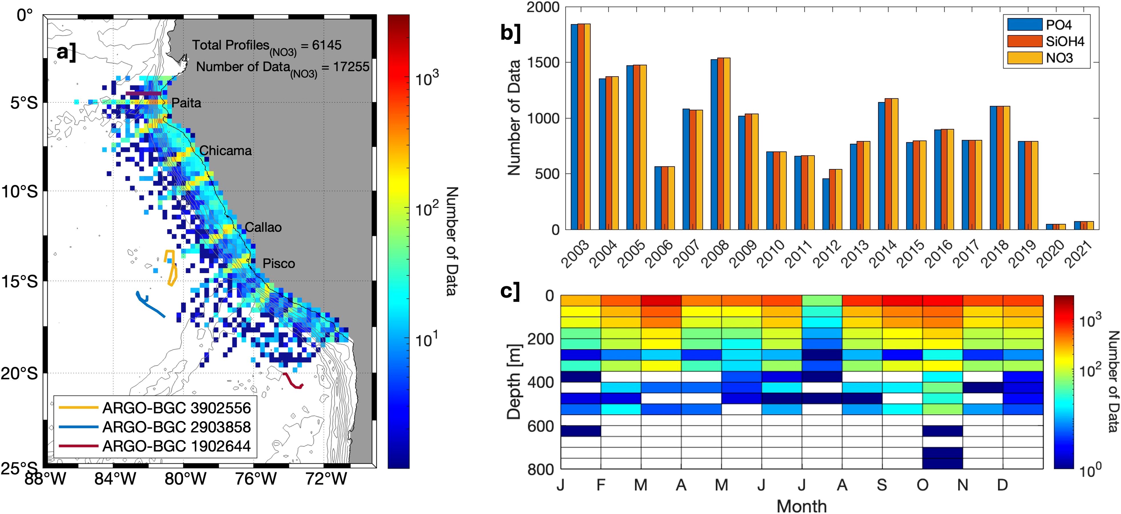
Figure 1. (a) Spatial distribution of $N{O}_3^{-}$ profiles binned in a 30 km grid where the color represents total density of data (#Data/30km) in log scale, (b) histogram of the total number of data available for $P{O}_4^{3-}$ (blue), $Si{(OH)}_4$ (orange), $N{O}_3^{-}$ (yellow) binned by year and (c) monthly distribution of the number of data binned in a 50 m vertical grid. The horizontal purple line in ~4.6 °S shows the path covered by the glider deployments.

2.1.2 Independent time series in Paita (5 °S) and Callao (12 °S)

A set of measurements was set aside and not used during the ANN training phase to serve as an independent validation of CANYON-PU. Four areas were defined off the shore of Paita (5 °S) and Callao (12 °S) where regular sampling is performed. This dataset contains a total of ~722 measurements from surface down to 500 m for each macronutrient and spans from 2003 to 2019 with a seasonal coverage that includes warm and cold conditions. Following the same criteria, the eligible data contains the core parameters as well as their corresponding nutrients. In order to test the general applicability of the method and its performance in coastal waters and in the open ocean, two zones along the cross-shore sections in front of Paita and Callao were selected. The available samples inside a 10 km radius at 81.45 °W, 5 °S and 82.5 °W, 5 °S corresponds to the independent dataset off Paita and, inside a 10 km radius at 77.3 °W, 12.2 °S and 78 °W, 12.5 °S, to Callao. The total dataset for Paita was 566 sampling points with a maximum depth of 500 m whereas, for Callao, was 156 points with profiles at standard levels that also reached 500 m at the most.

2.2 Artificial neural network architecture

Machine learning algorithms, such as ANN, have been widely used within the marine science community (Rubbens et al., 2023) and have shown promising results for classification and detection of plankton (Irisson et al., 2022). In recent years, the applications of ANN to estimate the nutrient concentration in the ocean have appeared (Bittig et al., 2018; Carter et al., 2021; Contractor and Roughan, 2021; Fourrier et al., 2020; Sauzède et al., 2017; Wang et al., 2023). Compared to the core variables such as temperature, salinity and oxygen and despite some development of ultraviolet profiling sensors (Daniel et al., 2020) that allows the measurement of $N{O}_3^{-}$, macronutrients concentrations are still largely undersampled which makes it a challenge to characterize their variability at high spatio-temporal scales. In this work, we propose a similar approach to CANYON (Sauzède et al., 2017), CANYON-B (Bittig et al., 2018) and CANYON-MED (Fourrier et al., 2020) by training an ANN with IMARPE’s biogeochemical dataset for the PUS region in order to estimate the concentration of $P{O}_4^{3-}$, $Si{(OH)}_4$ and $N{O}_3^{-}$.

2.2.1 Multilayer perceptron

Following CANYON methodology, we used a Multilayer Perceptron (MLP) to build the ANN. The MLP is a feed forward ANN with multiple hidden layers which has been shown capable of approximating a continuous function by connecting inputs and outputs (Bishop, 1995). The ANN functions iteratively connecting input data with values in the adjacent layer by weights that are readjusted in every iteration in order to minimize the error by decreasing the error function. Prior to the training phase, it is usually suggested that the data used is normalized between the range of -1 and 1 in order to improve the accuracy and efficiency of the model. The input data was normalized by following the same criteria as Fourrier et al. (2020) using the equation:

$\begin{array}{ll}x\text{'}= \frac{2}{3}*\frac{(x-\overline{x})}{\sigma }& (1)\end{array}$

Where x’ is the normalized input, x, $\underset{\_}{x}$ and $\sigma$ represent the input, its mean and the SD respectively. The factor ⅔ in Equation 1 allows that at least 80% of the data is restricted in the range [-1,1]. We used the Deep Learning Toolbox included in MATLAB to develop the MLP. Within the toolbox framework, we chose to randomly select 80% of the data to be used for the ANN training and 20% of the data to be used as validation. Validation within the training process ensures that there is iterative testing of the model using data that is not directly used in the training. For efficient computation, the ANN architecture was limited to two hidden layers, where the number of neurons in each layer could vary. The neuron count within each layer was randomized within the range of 1 to 50. Given the three distinct nutrients under investigation, we trained an independent MLP for each. To balance computational cost with a reasonable level of confidence in our final results, we performed 100 training runs for each nutrient, leading to a total of 300 trained ANN. Following the same steps detailed by Fourrier et al. (2020), we used a Bayesian Regularization Algorithm in order to appropriately determine the weights and errors during the training. After 100 training tests for each nutrient, we analyzed the performance of each ANN. This was done by computing the statistical metrics which evaluates the accuracy of the ANN on the validation datasets (20%): the Mean Absolute Error (MAE), Root Mean Squared Error (RMSE) and the Coefficient of determination (R²). These values were computed by comparing the ANN-retrieved nutrients and the corresponding in situ measurements and identifying the optimum configuration by choosing the highest R² and the lowest RMSE and MAE. Multiple single ANN can be combined to generate an ensemble model in order to improve the metrics of the estimated parameter (Linares-Rodriguez et al., 2013). Effectively, the approach applied to the Mediterranean Sea (Fourrier et al., 2020) combining the ten best nutrient outputs, based on R², showed higher correlation coefficients and lower errors in comparison with the performance of the best single model. Based on this evidence, the ensemble (ANN-E) shown in this paper averages the 10 best single outputs (ANN-1/10, Table 1).

Table 1

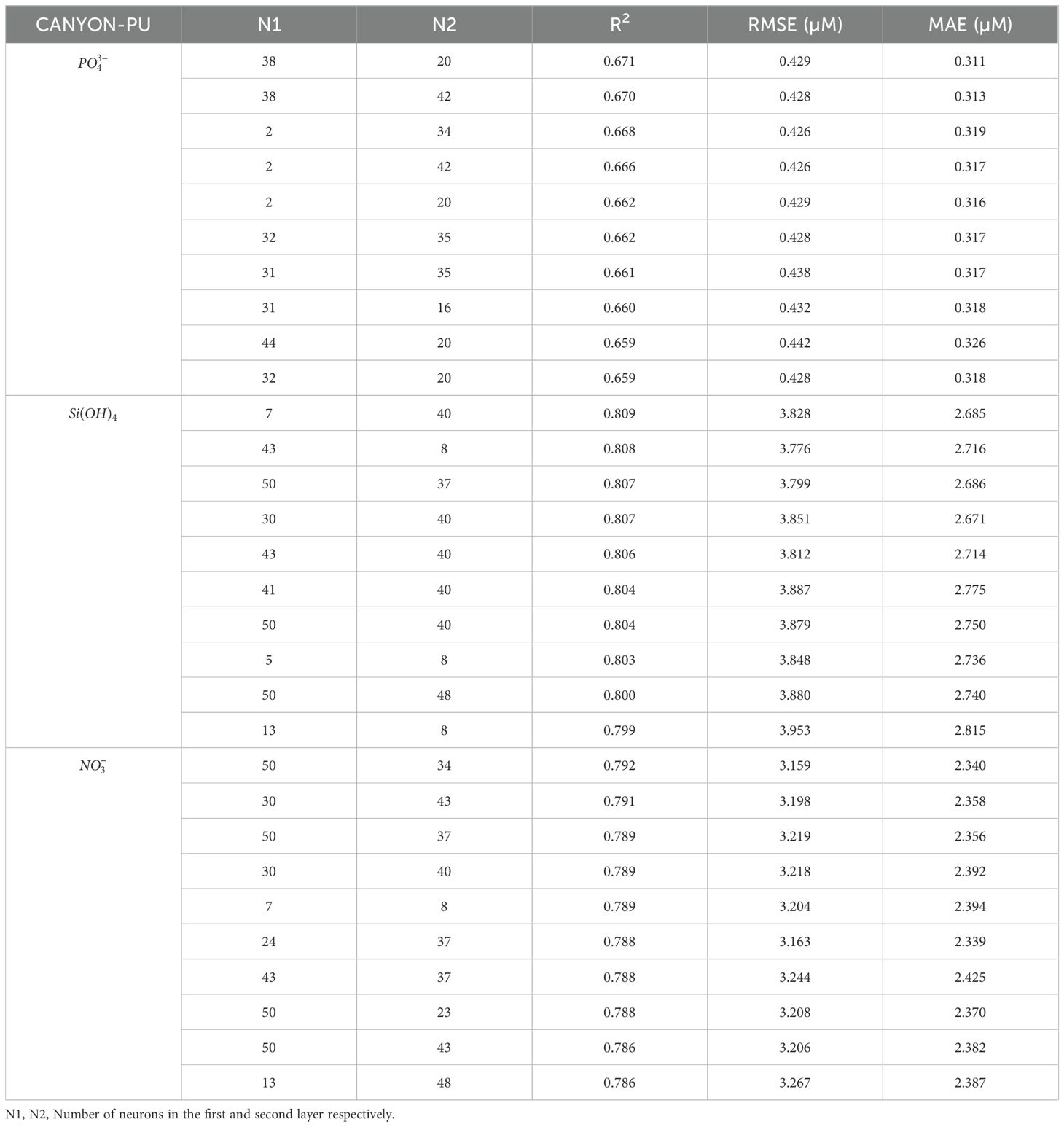
Table 1. 10 best performance CANYON-PU in the validation dataset (20%) for estimate $P{O}_4^{3-}$, $Si{(OH)}_4$ and $N{O}_3^{-}$.

2.2.2 Regionally trained ANN in the Peruvian upwelling system

Both CANYON and CANYON-B were trained using the Global Ocean Data Analysis Project version 2 (GLODAPv2) (Olsen et al., 2016), however, only CANYON-B is used in this study, as it represents an improved version of the initial CANYON model. The inputs CANYON-B uses to estimate the nutrients are latitude, longitude, date, depth, temperature, salinity and oxygen. The application of CANYON-B in the PUS showed poor performance based on the measured IMARPE values (Table 2). We attribute the poor performance of this model to the lack of observations available for the PUS and more broadly for the South Eastern Pacific region within the GLODAPv2 dataset. This motivated our work to train a regional ANN for the PUS, which we have named CANYON-PU. Our approach follows the regional adaptation of CANYON to the Mediterranean Sea by Fourrier et al. (2020). In addition to the potential temperature, salinity, oxygen, latitude, longitude, depth and day of the year, we tested the addition of four regionally relevant input parameters to train CANYON-PU: 1) The distance to the coast, 2) the bathymetry, 3) the Oceanic Niño Index (ONI) and 4) the Coastal El Niño Index (ICEN). The distance to the coast and the bathymetry associated with each sample was added due to the intense productivity gradient between the coast and the open ocean (Espinoza-Morriberón et al., 2017) and the influence of sediments from the continental platform in remineralization (Loginova et al., 2020). Also, ocean dynamics impacted by the presence of the continental slopes are important for the propagation of coastal trapped waves and potentially nutrient distribution (Pietri et al., 2014). The distance to the coast was computed using the minimum distance between the coastline and the sampling point. The bathymetry used was GEBCO_2023: a global terrain model that provides elevation data on a 15 arc-second interval grid (Tozer et al., 2019). Furthermore, the PUS being highly susceptible to interannual events such as El Niño Southern Oscillation (ENSO) (Arntz et al., 2006; Espinoza-Morriberón et al., 2017; Peng et al., 2024) led us to include two indices developed to characterize it. The index built to characterize warmer or colder conditions in the region El Niño 3.4 (5 °N-5 °S, 120 °W-170 °W) denominated the ONI index was developed by NOAA. It is defined as a set of 3-month running averages of sea surface temperature(SST) anomalies in the region 5 °N-5 °S, 120 °W-170 °W (Huang et al., 2017) and characterizes warm (El Niño) or cold (La Niña) conditions based on a threshold of +/- 0.5 °C. While the ONI index is a helpful tool for identifying typical ENSO events in the Central Pacific (Takahashi et al., 2011), studies have also shown unusual instances of significant warming along the Peruvian coast even when the Central Pacific stayed cooler (Echevin et al., 2018; Peng et al., 2024). Therefore, we included an additional index for the El Niño 1+2 region (0 -10 °S, 90 °W-80 °W) denominated ICEN. This index developed by the Peruvian Commission for the Study of El Niño (ENFEN) is a monthly index computed using a 3-month moving average of SST anomalies from ERSSTv5 (Huang et al., 2017). It distinguishes warm or cold conditions based on a threshold of +0.5 °C and -1.2 °C respectively. Although both ONI and ICEN indices are useful to characterize canonical ENSO events (Takahashi et al., 2011), the ICEN has shown a better representation of less frequent and peculiar events in the PUS such as the coastal El Niño in 2017 and 2023 (Echevin et al., 2018; Peng et al., 2024).

Table 2

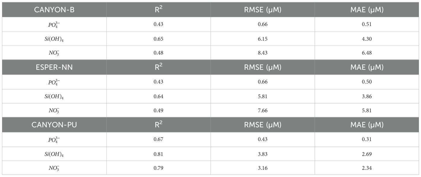
Table 2. Performance of CANYON-B, ESPER-NN and CANYON-PU in the validation dataset (20%) for estimate $P{O}_4^{3-}$, $Si{(OH)}_4$ and $N{O}_3^{-}$.

2.3 Other sources of hydrographic and biogeochemical data: GLODAPv2.2023, IMARPE climatology and BGC-Argo

In order to assess the reliability of the model’s estimation aside from OSD samples, we used three different external data sources: i) GLODAPv2.2023, ii) IMARPE monthly climatology and iii) BGC-Argo floats.

Recently the GLODAPv2 (Olsen et al., 2016) used in the training of the original CANYON-B has been updated and distributed as GLODAPv2.2023 (Lauvset et al., 2024). The key feature of this update is the availability of three cruises with samples at maximum depths of 5500 m in the central and southern margin of the PUS that were not included in GLODAPv2 (Figure 1a). GLODAP employs rigorous quality control procedures, including crossover analysis and bias adjustments, to achieve a target consistency of 2% for $P{O}_4^{3-}$, $Si{(OH)}_4$ and $N{O}_3^{-}$ concentrations across its global dataset (Lauvset et al., 2024). The resulting statistical characteristics (in µM) for these nutrients in the GLODAPv2.2023 dataset are summarized as follows: $P{O}_4^{3-}$ (mean: 2.3, median: 2.5, SD: 0.59), $Si{(OH)}_4$ (mean: 20.95, median: 24.93, SD: 10.47), and $N{O}_3^{-}$ (mean: 20.47, median: 20.87, SD: 8.67).

Additionally, a monthly T-S-O₂ climatology (1981-2010) developed by IMARPE (Grados et al., 2018) was used in order to show the capability to reconstruct the seasonal variability of the estimated nutrients and it was compared with IMARPE’s nutrient climatology (Espinoza-Morriberón et al., 2017) displayed in a gridded field of 0.25° x 0.25° and in 55 vertical levels between surface and 1000 m the same spatial resolution as the T-S-O₂ gridded field. The nutrient climatology provided the following key metrics (in µM): $P{O}_4^{3-}$ (mean: 2.31, median: 2.42, SD: 0.64), $Si{(OH)}_4$ (mean: 28.76, median: 24.02, SD: 19.55), and $N{O}_3^{-}$ (mean: 22.49, median: 20.58, SD: 11.47). Another source of biogeochemical data for further validation of CANYON-PU, available since the end of 2023, is the dataset from three Biogeochemical Argo floats (BGC-Argo; Claustre et al., 2020; Wong et al., 2020) equipped with $N{O}_3^{-}$ SUNA sensors drifting along the central-southern Peruvian coast. Following quality control procedures, the estimated error found for these nitrate measurements is typically ±0.5 µM (Claustre et al., 2020). The float World Meteorological Numbers (WMO) 3902556 located in the central Peruvian coast and the floats WMO 2903858 and 1902644 located in the southern Peruvian coast (Figure 1a) began their measurements on December of 2023 collecting profiles at a 10 day frequency through March 2024 when the data was accessed for this study. The vertical sampling of BGC-Argo profiles reaches ~2000 m with a resolution of 2m enabling them to estimate $N{O}_3^{-}$ at fine scales. The analysis in this work focused on the delayed-mode quality controlled profiles that were chosen with a flag of 1 (i.e. good data) and at a maximum depth of 500 m. The $N{O}_3^{-}$ data collected by BGC-Argo floats provided the following descriptive statistics (mean, median, and SD in µM): WMO 3902556 (22.64, 22.16, 12.16), WMO 2903858 (17.28, 16.84, 13.95), and WMO 1902644 (19.66, 12.81, 14.38).

2.4 Gliders dataset

This work also relies on a test application of CANYON-PU on glider dataset. Over the past 15 years, several Slocum gliders were deployed across-shore in the PUS (Pietri et al., 2014, 2013; Thomsen et al., 2016) recording relatively high-resolution vertical profiles of the water column down to a maximum depth of 1000 m (Testor et al., 2018). All the vehicles were equipped with a CTD and an optode for measuring oxygen, providing a finer spatio-temporal resolution for the application of CANYON-PU. In this work, we used data from two missions deployed in the northern Peruvian coast (~4.6 °S, Figure 1a) during December of 2022 and March of 2023 with a maximum depth of 400 m in order to illustrate possible application of CANYON-PU to high resolution glider data. Each T-S-O₂ profile collected by the glider was analyzed to remove statistical outliers. These periods represented the conditions before and during the peak of El Niño event 2023 (Peng et al., 2024).

3 Results

The capability of CANYON-PU to estimate $P{O}_4^{3-}$, $Si{(OH)}_4$ and $N{O}_3^{-}$ concentrations in the PUS are tested using a validation dataset corresponding to the 20% of all the samples available. Additionally, when comparing the outputs against CANYON-B and ESPER-NN, it shows a significant overall improvement as indicated by higher R² values, and lower RMSE and MAE metrics (Table 2). The high R² values represent a good fit between CANYON-PU and the measurements, while the lower errors give information about the accurate prediction of our model. Furthermore, CANYON-PU can represent with better accuracy the nutrients in the upper 25 m due to the large availability of surface data during its training.

3.1 CANYON-PU overall performance in the Peruvian upwelling system

In general, CANYON-B and ESPER-NN have provide good estimations for the principal macronutrients in the global oceans (Bittig et al., 2018; Carter et al., 2021). For example, the RMSE for CANYON-B reported by Bittig et al. (2018) is 0.051 µM ($P{O}_4^{3-}$), 2.3 µM ($Si{(OH)}_4$) and 0.68 µM ($N{O}_3^{-}$). Carter et al. (2021) reported a similar RMSE for ESPER-NN, specifically: 0.043 µM ($P{O}_4^{3-}$), 2.0 µM ($Si{(OH)}_4$) and 0.56 µM ($N{O}_3^{-}$). However, when it was tested in the PUS, the RMSE increased to 0.66 µM ($P{O}_4^{3-}$), 6.15 µM ($Si{(OH)}_4$) and 8.43 µM ($N{O}_3^{-}$) (Table 2). This could be related to the scarcity of the data in the region used for the training of CANYON-B and ESPER-NN. and the large natural variability of nutrient concentration in the PUS. Effectively, the R² values varies for each nutrient, with $Si{(OH)}_4$ having the highest (0.65), while the values for $P{O}_4^{3-}$ and $N{O}_3^{-}$ (0.43 and 0.48 respectively) were lower. In contrast, the performance of CANYON-PU was better for all the three nutrients (Table 2) when applied to the same validation dataset. Moreover, the errors were, in general, 50% lower which evidenced the good performance due to the use of the regional dataset during the training phase of the model. The variations in performance for each nutrient predicted by the CANYON-PU model (Table 2), as indicated by different R² values, reflect the diverse physical and biological processes that govern the variability of each nutrient in the PUS (Pennington et al., 2006). For example, $P{O}_4^{3-}$ shows lower R² coefficient (0.67) whereas $Si{(OH)}_4$ and $N{O}_3^{-}$ were considerably higher (0.81 and 0.79 respectively). Although the latter reflects a good performance in the validation dataset above 300 m, in the layer between 400–500 m there was some bias between the estimated value and the in situ measurements, which reflects the impact of the scarcity of samples below that level during the training (Figure 2).

Figure 2

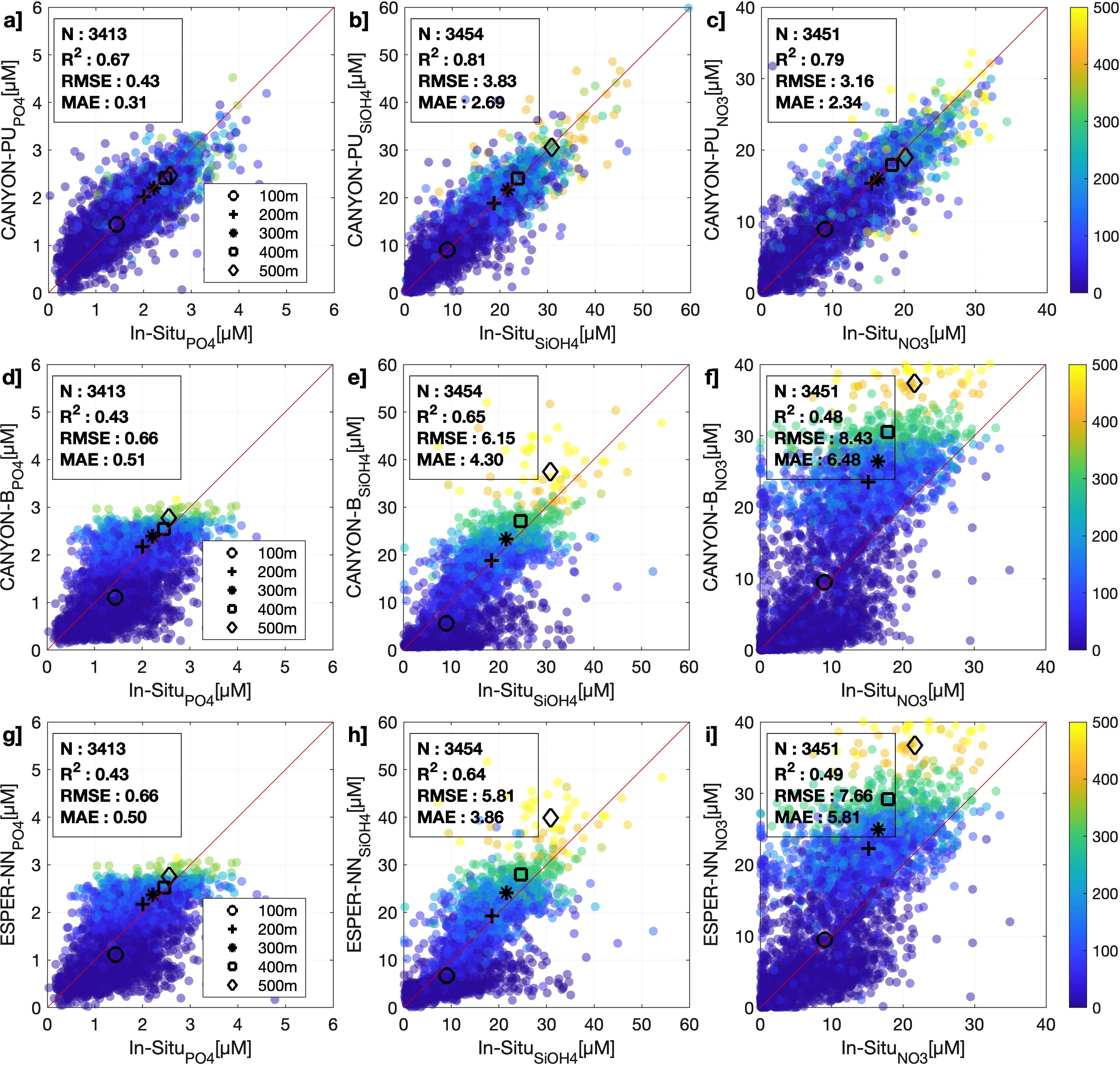
Figure 2. Scatterplot of validation dataset (20%) between in situ values against estimated of (a) $P{O}_4^{3-}$, (b) $Si{(OH)}_4$ and (c) $N{O}_3^{-}$ from (a-c) CANYON-PU, (d-f) CANYON-B and (g-i) ESPER-NN. The color represents the depth for each compared sample. The black markers show the averaged nutrient in a layer of 0–100 m, 100–200 m, 200–300 m, 300–400 m and 400–500 m. The slope chosen as the reference line is 1 (red).

The relative and absolute differences between CANYON-PU and validation in situ dataset are shown on Figure 3 along vertical profiles. The relative variation is represented in percentage so that positive (negative) values represent an overestimation (underestimation) of the ANN. For all three nutrients it is noticeable that in the upper layers, above 50 m, concentrations are overestimated which likely reflects the highly variable nature of the system (Lüdke et al., 2019) and CANYON-PU cannot account for factors such as nutrient depletion, for example. The vertical differences (Figure 3) averaged by depth shows slight variations in $Si{(OH)}_4$ accordingly with the high R², whereas for $P{O}_4^{3-}$ and $N{O}_3^{-}$ are noticeably underestimated by CANYON-PU below 200 m and 100 m respectively. Although the differences increased with depth, the relative differences showed values in the range +/- 10% confirming the robustness of CANYON-PU. That being said, we observed some relative positive outliers probably appeared due to sample contamination which causes nutrient consumption especially at higher concentrations (Dore et al., 1996).

Figure 3

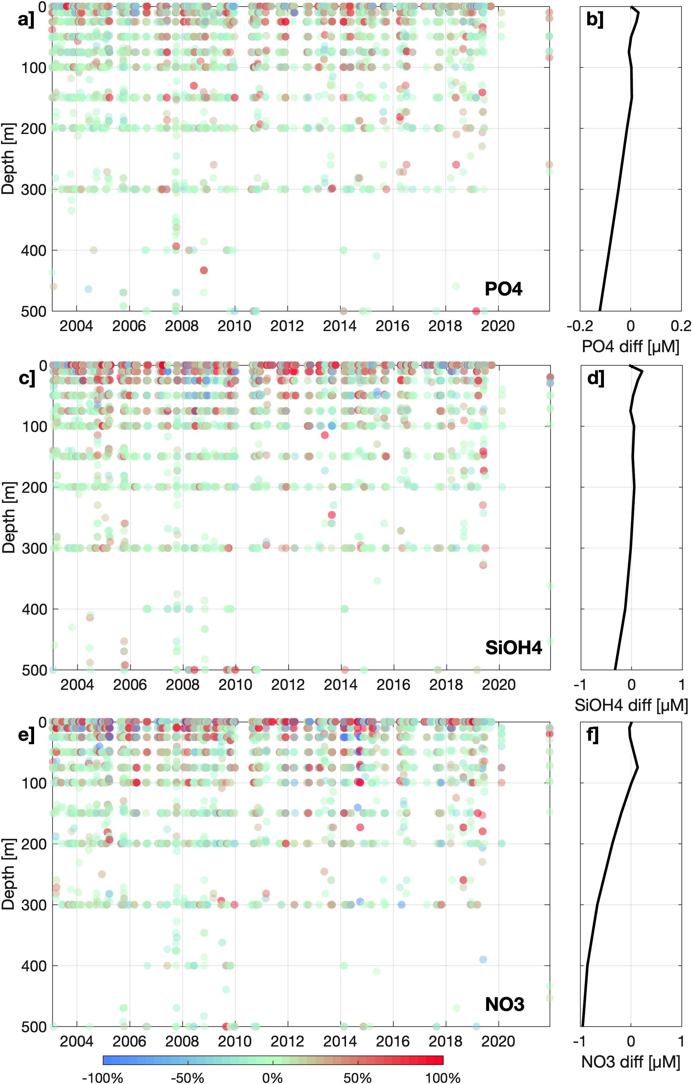
Figure 3. Validation dataset (20%)’s relative difference (%) between the output from CANYON-PU and in situ values for (a) $P{O}_4^{3-}$, (c) $Si{(OH)}_4$ and (e) $N{O}_3^{-}$. The corresponding averaged difference (µM) is shown in panels (b), (d, f).

3.2 Performance of CANYON-PU with independent datasets

3.2.1 Sampling stations in Paita and Callao

The independent datasets in Paita and Callao are used as a further validation of CANYON-PU accuracy (Figure 4). Effectively, the best performance ANN configuration from CANYON-PU (i.e. ANN-1) was similar when it was applied to the 20% validation dataset used in Section 3.1. Table 3 shows the R² for the ANN-1, $Si{(OH)}_4$ showed the highest correlation coefficient (0.79), followed by $N{O}_3^{-}$ (0.68) and $P{O}_4^{3-}$ (0.58). Although the performance from ANN-1 highlights the robustness of our method, the ANN-E showed even higher correlations. In general, the ANN-E improves the correlation coefficient by 6% and lowered the errors (Table 3). This is consistent with the results obtained by Fourrier et al. (2020) in a similar study for the Mediterranean Sea. Additionally, the relative differences seen in vertical profiles (Figure 5) were less than 10% in general. For the upper 100 m layer, it was close to 8% for $P{O}_4^{3-}$ and $Si{(OH)}_4$ and 11.9% for $N{O}_3^{-}$. Moreover, the deeper layers showed even less differences near 3% ($P{O}_4^{3-}$) with $N{O}_3^{-}$ being the highest at 8%. The latter supports our premise that the ANN-E shows an increased performance and could be used in the other datasets.

Figure 4

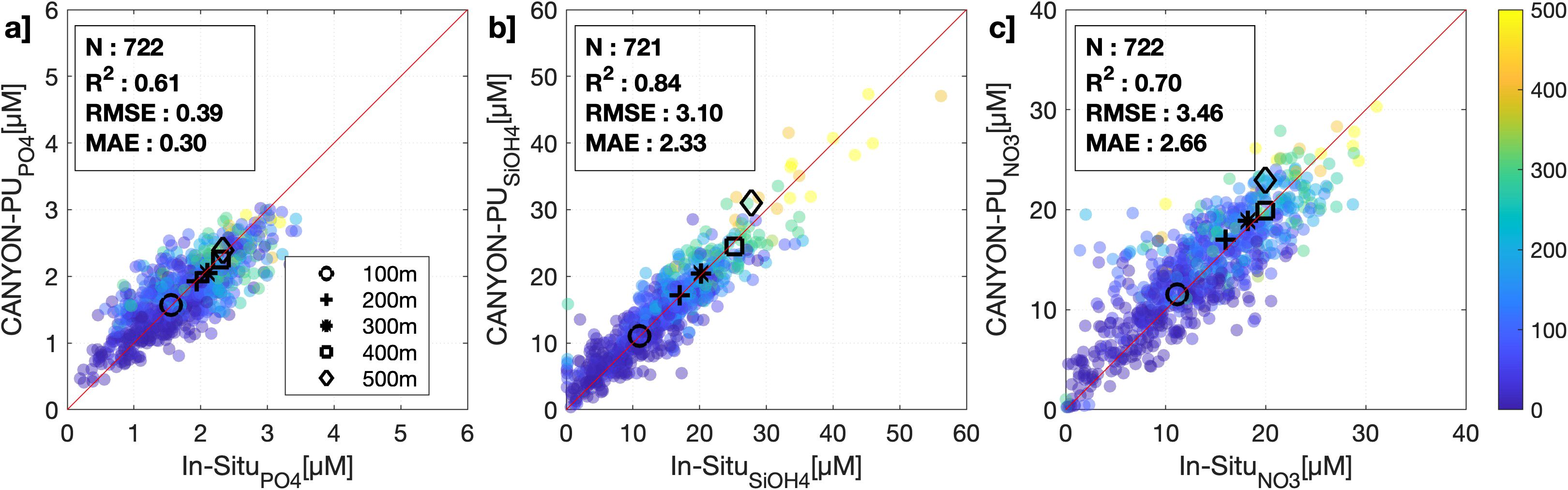
Figure 4. Scatterplot of independent validation dataset (Paita and Callao) between in situ values against CANYON-PU. (a) $P{O}_4^{3-}$, (b) $Si{(OH)}_4$ and (c) $N{O}_3^{-}$. The color represents the depth for each compared sample. The black markers show the averaged nutrient in a layer of 0–100 m, 100–200 m, 200–300 m, 300–400 m and 400–500 m. The slope chosen as the reference line is 1 (red).

Table 3

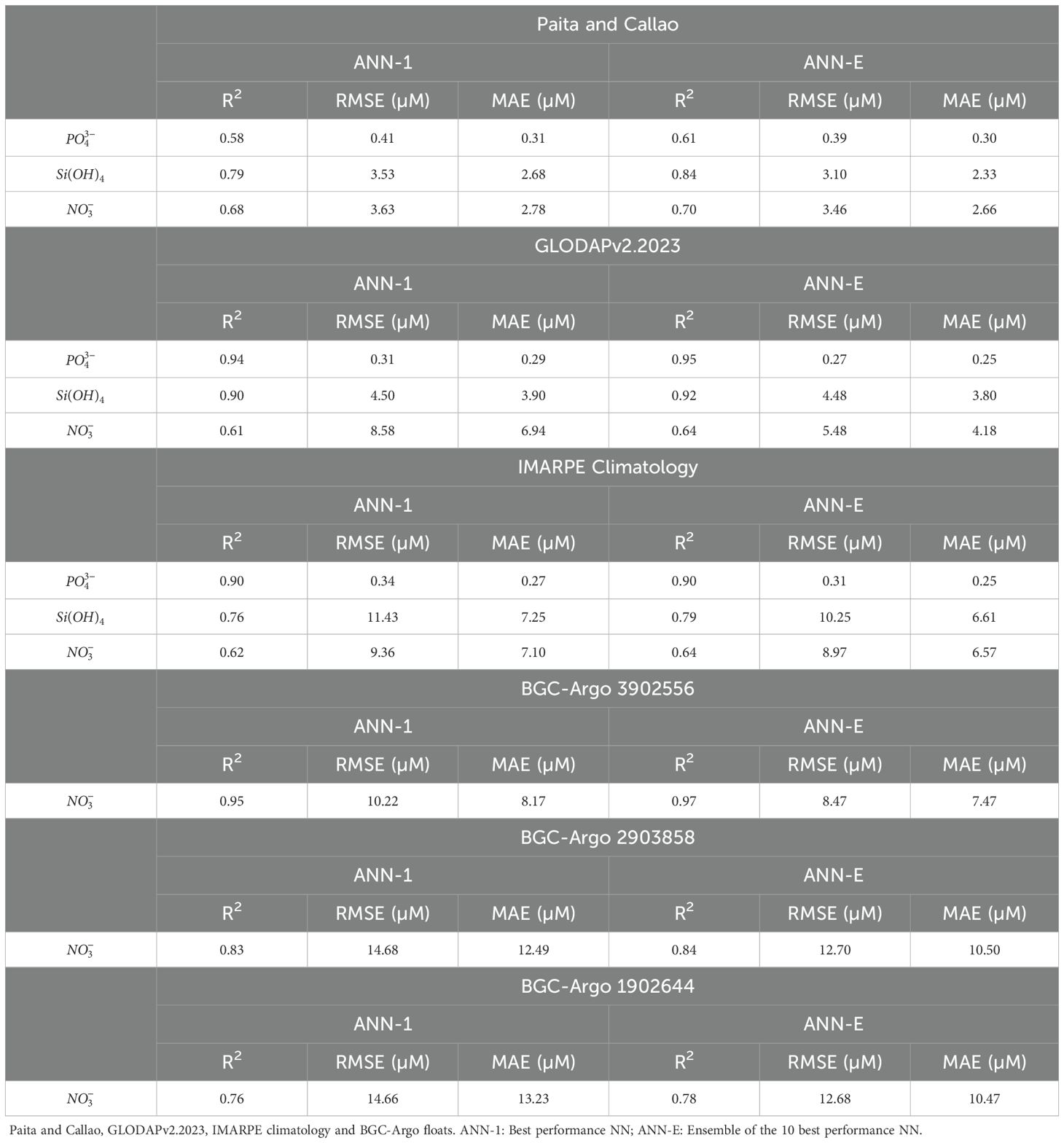
Table 3. Metrics for independent validation datasets.

Figure 5

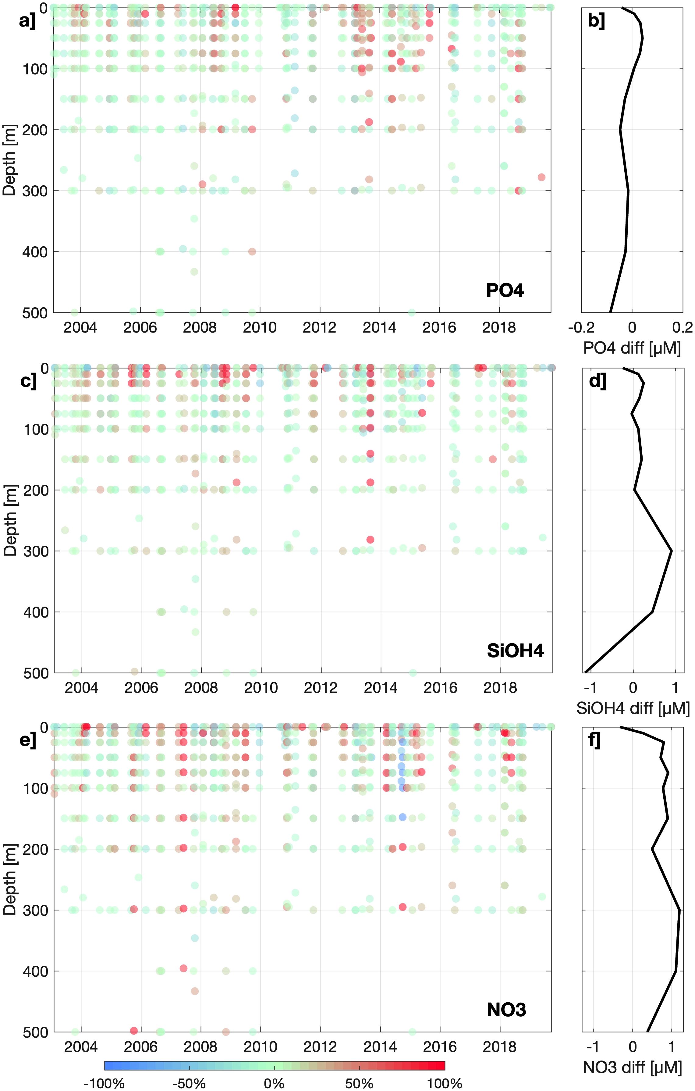
Figure 5. Paita and Callao independent validation dataset’s relative difference (%) between the output from CANYON-PU and in situ values for (a) $P{O}_4^{3-}$, (c) $Si{(OH)}_4$ and (e) $N{O}_3^{-}$. The corresponding averaged difference (µM) is shown in panels (b, d, f).

3.2.2 GLODAPv2.2023

The performance achieved by CANYON-PU after applying it on the GLODAPv2.2023 profiles that were inside the training area (Figure 6) demonstrates better overall performance relative to the independent validation dataset of Paita and Callao. Effectively, the R² coefficient for $P{O}_4^{3-}$ (0.95) and $Si{(OH)}_4$ (0.92) are higher, whereas for $N{O}_3^{-}$ is lower (0.64). The observed difference in R² is likely linked to the differing inherent variability of the validation datasets. The longer time series from Paita and Callao (2003-2021, all seasons) likely exhibits greater natural variability than the GLODAPv2.2023 data (austral spring/summer 2013, 2017). The comparable RMSE and MAE values (Table 3) confirm the model’s consistent absolute error magnitude, suggesting the variation in R² is a consequence of evaluating against datasets with different total variance. On the other hand, for the three estimated nutrients we find a linear correlation in the first 100 m that slightly leans towards an underestimation of 20% between 200–500 m and more evident in $N{O}_3^{-}$ which additionally shows higher errors. A further analysis demonstrates that considering the GLODAPv2.2023 profiles outside the training area 400 km offshore is slightly detrimental to CANYON-PU in $P{O}_4^{3-}$ and $Si{(OH)}_4$ reliability lowering the R² to 0.93 and 0.89 respectively. However, for $N{O}_3^{-}$ our analysis demonstrates better performance highlighted by an R² of 0.83. This could be related to some processes near the coast that cannot be represented by the ANN. Overall, we have noticed that including profiles below 500 m greatly increases the systematic bias, which might suggest a limit for applicability of CANYON-PU below this depth (coherent with sampling distribution of the training data set).

Figure 6

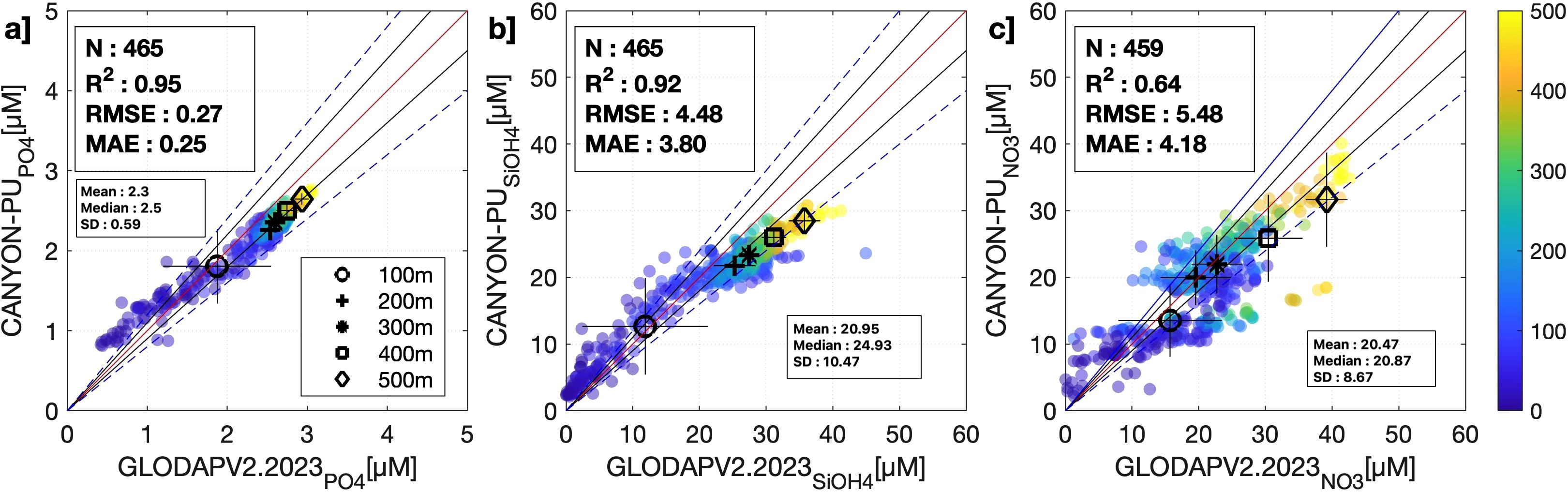
Figure 6. Scatter plot of GLODAPv2.2023 against CANYON-PU. (a) $P{O}_4^{3-}$, (b) $Si{(OH)}_4$ and (c) $N{O}_3^{-}$. The color represents the depth for each compared sample. The black markers show the averaged nutrient in a layer of 0–100 m, 100–200 m, 200–300 m, 300–400 m, 400–500 m and the lines on top, the SD. The slopes chosen as the reference lines are 1 (red line), 0.9/1.1 (black line) and 0.8/1.2 (blue dashed line). The Mean, Median and SD for GLODAPv2.2023 are shown in the small boxes.

3.2.3 IMARPE climatology

The capability of CANYON-PU to represent nutrients at a different time scale was tested using a T-S-O₂ monthly gridded climatology as input. Additionally, the outputs were compared against IMARPE’s $P{O}_4^{3-}$, $Si{(OH)}_4$ and $N{O}_3^{-}$ climatology that is gridded at the same spatial scale as the inputs. The outputs from CANYON-PU for $P{O}_4^{3-}$ and $Si{(OH)}_4$ show a low bias when it was compared against the climatology (Figures 7a, b). Effectively, the previous statement was reflected in a high R² of 0.9 for $P{O}_4^{3-}$ and 0.79 for $Si{(OH)}_4$. Although the correlations showed a good performance in the deeper layers, the upper 100 m was overestimated in CANYON-PU through all the months. Moreover, the performance for $N{O}_3^{-}$ was lower with a R² of 0.64 which was due to a higher relative difference in the first 200 m. The climatology of $N{O}_3^{-}$ also reveals that from austral spring to summer the underestimation from CANYON-PU reached the layer over 400 m. In general, $P{O}_4^{3-}$ and $Si{(OH)}_4$were represented with more precision and confirmed the conservative nature of $Si{(OH)}_4$ whereas the processes of consumption and depletion of nitrogen were difficult to capture by CANYON-PU impacting on the robustness of $N{O}_3^{-}$ estimation.

Figure 7

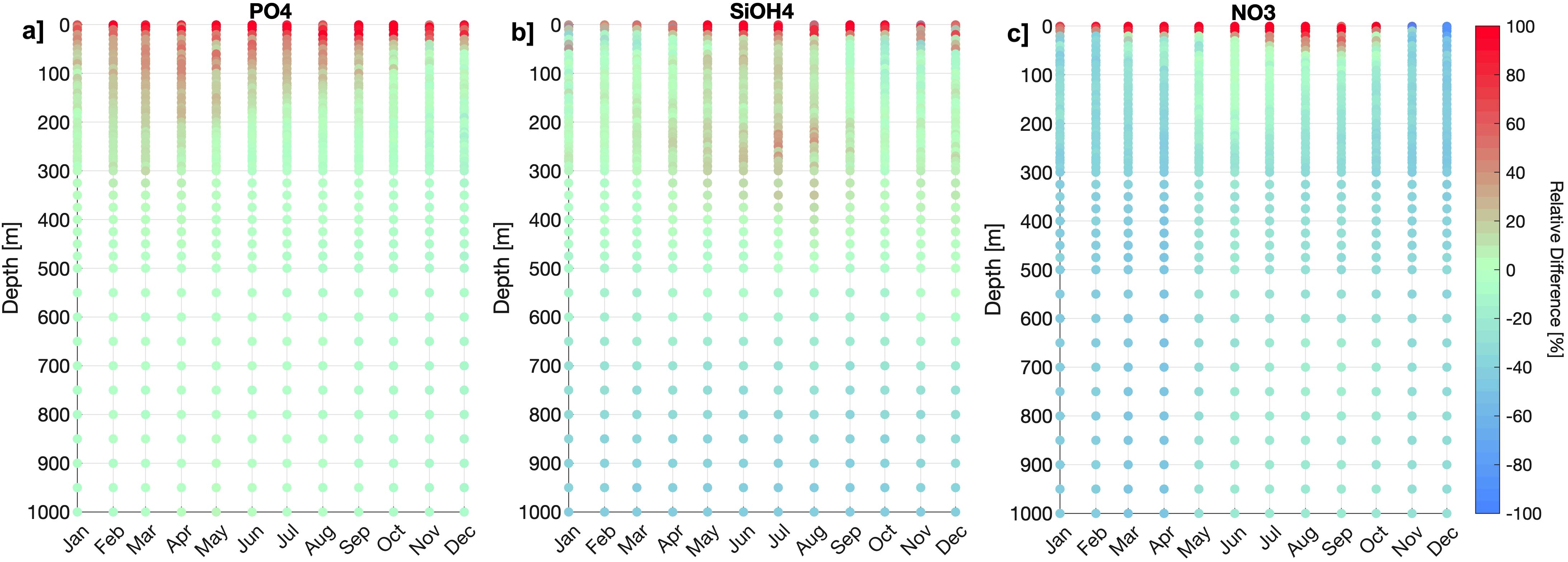
Figure 7. Relative difference (%) obtained from the output of CANYON-PU and nutrient monthly climatology for (a) $P{O}_4^{3-}$, (b) $Si{(OH)}_4$ and (c) $N{O}_3^{-}$.

3.2.4 BGC-Argo floats

The three drifting BGC-Argo floats with $N{O}_3^{-}$ measurements, located 400 km offshore the central-south Peruvian coast (Figure 1a) were used to test CANYON-PU and evaluate its robustness using a dataset with a different spatio-temporal scale.

The difference between the estimated and measured $N{O}_3^{-}$ (Figure 8) shows a similar pattern in the first 500 m for all the BGC-Argo floats analyzed. Effectively, floats 3902556, 2903858 and 1902644 measured higher nutrients compared to CANYON-PU in the first 50 m, this difference increased rapidly until 100 m, especially for float 1902644. Below 100 m a decrease in the difference can be noted, reaching its minimum value at 200 m, principally for float 3902556. The relatively low error remains until 325 m where an increment is again observed reaching a maximum of -17 µM at 500 m. In general, CANYON-PU underestimates all Argo float samples specially for float N° 1902644 which was located at the southernmost domain of training dataset available. This shows that, due to the lack of data in that area, CANYON-PU cannot accurately represent the relatively high values observed which led to an underestimation. On the other hand, float 3902556, although being outside of the available training domain, was relatively closer to a dense area of training points that probably affected positively the performance. Similarly float 29030858 was located a few degrees west of the available training domain, close to a sufficient amount of training points. In general, the comparison showed a high R² of 0.97 and an RMSE and MAE of 8.47 and 7.47 respectively.

Figure 8

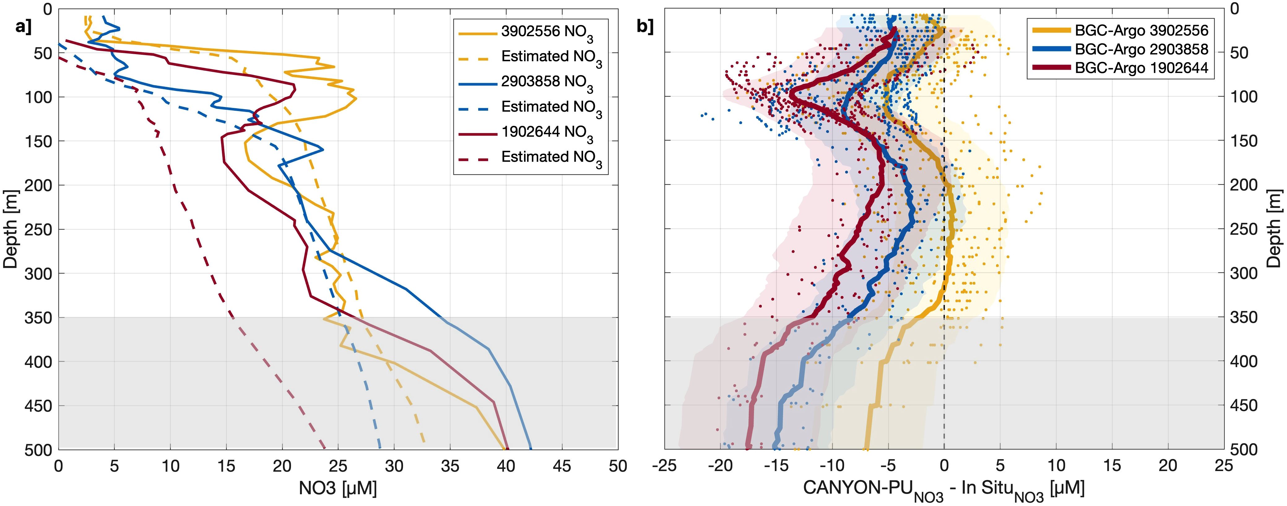
Figure 8. (a) Vertical profile of $N{O}_3^{-}$ for cycle 4 (thin lines) in BGC-Argo float 3902556 (yellow), 2903858 (blue) and 1902644 (red) and the corresponding estimate (dashed lines) from CANYON-PU. (b) Vertical profiles of $N{O}_3^{-}$ difference (µM) between CANYON-PU and BGC-Argo (color dots). The shadings represent the ± 1 SD. The thick colored lines are the averaged difference for the corresponding BGC-Argo float. The grey shading below 350 m represents the layer with low accuracy.

3.3 Example application: gliders

A further application of CANYON-PU was tested using two glider deployments in the northern Peruvian coast (Talara, ~4.6°S). The periods covered by those missions were November 2022 and March 2023 corresponding to the onset and progression of an El Niño event (Figure 9).

Figure 9

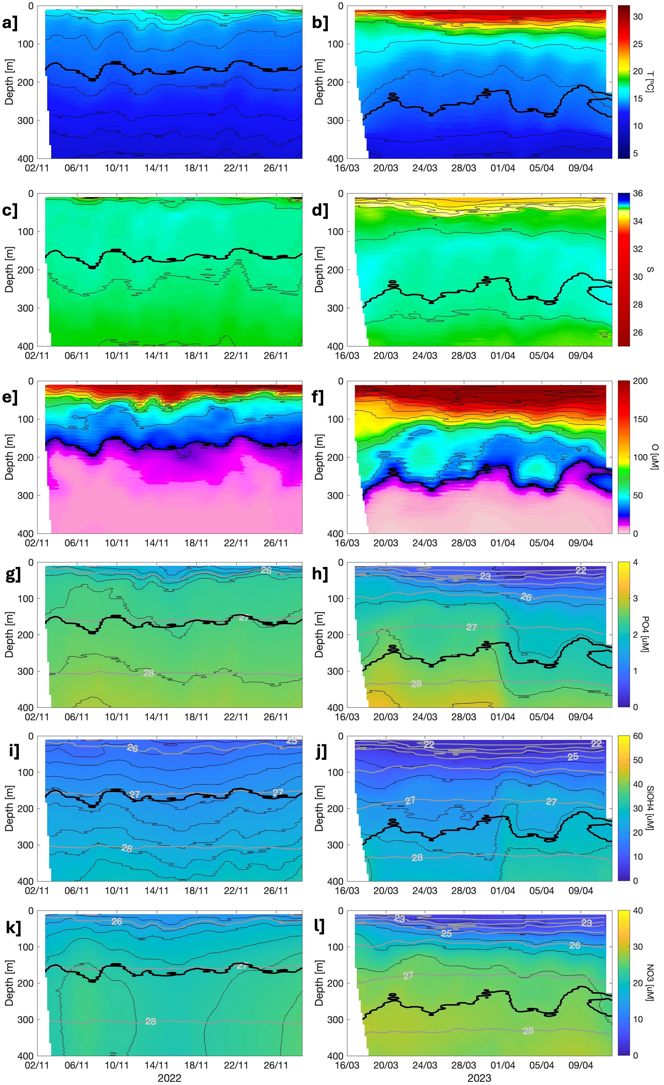
Figure 9. Glider measurements before (left panel) and during (right panel) El Niño event in 2022-2023. Panels (a-f) represent the T-S-O2 fields and nutrients in (g, h) $P{O}_4^{3-}$, (i, j) $Si{(OH)}_4$ and (k, l) $N{O}_3^{-}$ estimated with CANYON-PU. Contours between (g-l) are the density fields in (kg/m³). The thick black line represents the upper limit of the OMZ (< 22 µM).

The T-S-O₂ fields show a noticeably heterogeneous distribution; for temperature, there was a slight increase by the end of 2022 that rose considerably by March 2023 and reached its peak of 30 °C in April. Associated with this, an intrusion of Tropical and Equatorial Surface Water (S<33.5 and S<34.8 respectively) was observed in the salinity fields. The upper limit of the OMZ (O<22 µM, Espinoza-Morriberón et al., 2021) deepened ~100 m while the El Niño event was at its peak. Moreover, the upper layers were more oxygenated than their counterparts in November-December 2022.

The estimated nutrients from CANYON-PU under these settings are shown in Figures 9g–l revealing a general depletion of nutrients, primarily in the upper 200 m, when the El Niño event was active. It is also observed that the high stratification is closely related to the consumption of $P{O}_4^{3-}$ and $N{O}_3^{-}$ consistent with previous studies in other regions (Tozawa et al., 2024), whereas $Si{(OH)}_4,$ was depleted in the whole water column. The descriptive statistics (mean, median, and SD in µM) for the estimated $P{O}_4^{3-}$, $Si{(OH)}_4^{}$, and $N{O}_3^{-}$ for the two periods were as follows: for 2022, values were $P{O}_4^{3-}$ (2.43, 2.47, 0.26), $Si{(OH)}_4$ (21.13, 21.5, 4.85), and $N{O}_3^{-}$ (20.69, 21.46, 2.7); while for 2023, the corresponding values were $P{O}_4^{3-}$ (2.04, 2.16, 0.65), $Si{(OH)}_4$ (20.15, 22.25, 8.5), and $N{O}_3^{-}$ (22.55, 25.56, 6.81).

This demonstrates the ability of CANYON-PU to estimate and represent reasonable features of nutrient distribution under different climate forcings, confirming its potential applicability to diverse datasets, including high resolution data collected by gliders.

4 Discussion

4.1 CANYON-PU performance under different settings

The process of testing which parameter has the most impact in the performance of CANYON-PU was achieved by zeroing one by one each parameter used in the training step. We then applied our ANN to predict the nutrient concentration under different scenarios and compared the R² in each case (Figure 10). First, under the assumption that a correlation value over 0.4 for $P{O}_4^{3-}$ is considered an improvement over CANYON-B, parameters such as pressure, bathymetry, distance to the coast and salinity had low impact in the ANN accuracy whereas variables like day of the year, latitude, longitude, potential temperature, El Niño 1+2 and El Niño 3.4 indices had the strongest impact on the R² values, rendering them as low as 0.1. The day of the year had the greatest impact over all the 10 best model configurations, with latitude following closely. These parameters were already included in the training of CANYON-B and it was expected that the seasonality and the position played a key role in the nutrient estimation. However, both El Niño indices that were incorporated only in CANYON-PUS, followed as important parameters having significant impact in lowering the R² to 0.15. The latter confirms our previous assumptions that led us to include those indices in the training; the high susceptibility of the region to ENSO events (Arntz et al., 2006; Espinoza-Morriberón et al., 2017; Peng et al., 2024). Furthermore, the potential temperature generated a highly variable correlation coefficient in the model which could reveal that it might be particularly sensitive to thermal changes.

Figure 10

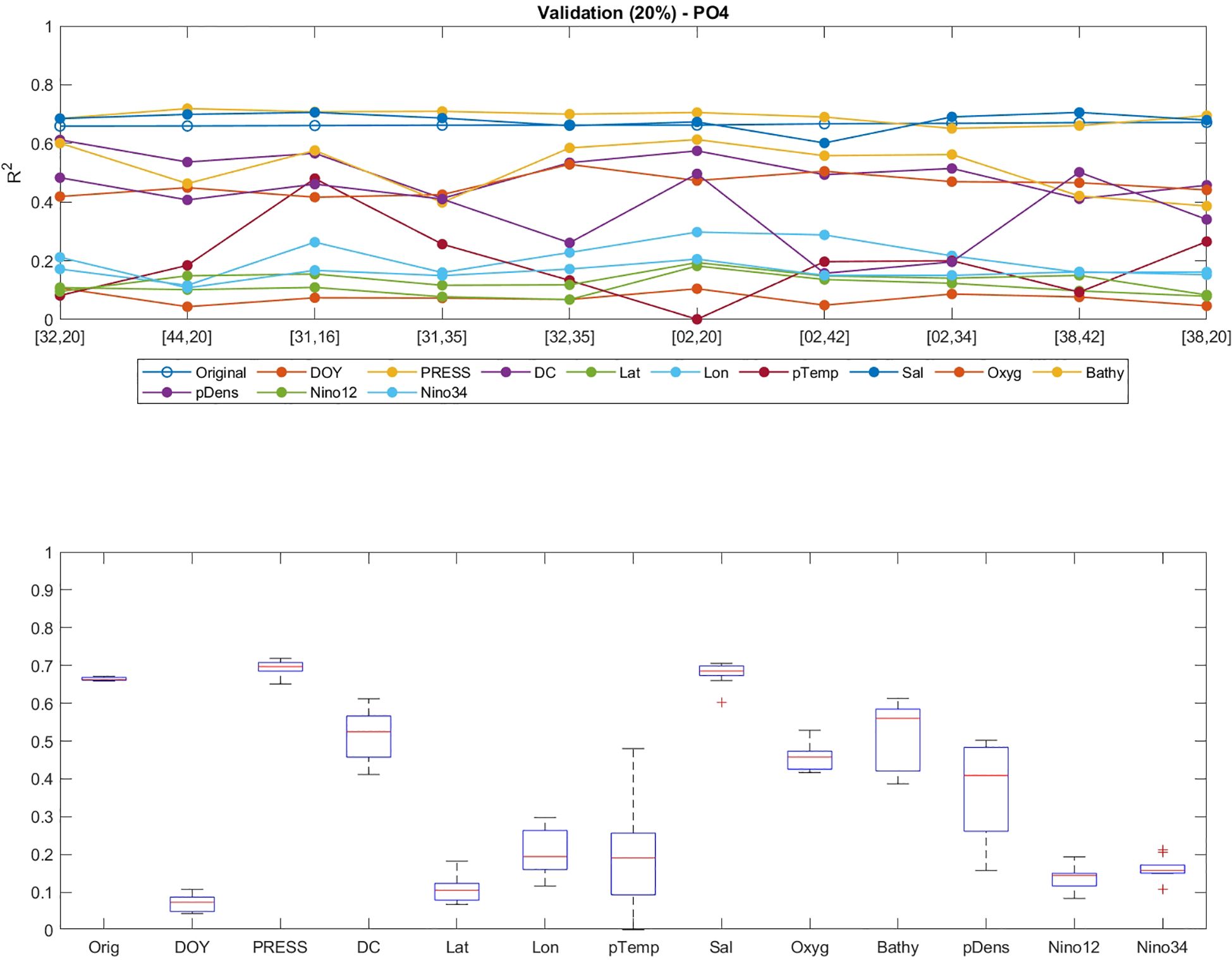
Figure 10. Model performance for the validation dataset (20%) of $P{O}_4^{3-}$ represented by the R² values (upper panel) for the 10 best configurations (numbers in brackets represent the amount of neurons in the first and second hidden layers) under different scenarios after the indicated parameter was zeroed. The lower panel shows the boxplot of all 10 best R² values when each parameter (indicated in the X-axis) was zeroed. Orig, Original; DOY, Day Of the Year; PRESS, Pressure; DC, Distance to Coast; Lat, Latitude; Lon, Longitude; pTemp, Potential Temperature; Sal, Salinity; Oxyg, Oxygen; Bathy, Bathymetry, pDens, Potential Density; Nino12, ICEN Index; Nino34, ONI Index.

4.2 Capability of nutrient estimation at different scales

The performance of CANYON-PU over different datasets has generally shown better results than CANYON-B and could help to represent the nutrient distribution in a highly variable environment such as the PUS (Echevin et al., 2018, 2014; Lüdke et al., 2019). Effectively, when the ensemble of CANYON-PU (ANN-E) was applied to bottle samples mostly at standard depths, it increased the R² over 45% and lowered the RMSE (MAE) by 0.24 µM (0.2 µM), 2.18 µM (1.57 µM) and 5.25 µM (4.17 µM) for $P{O}_4^{3-}$, $Si{(OH)}_4$ and $N{O}_3^{-}$ respectively. Moreover, these errors showed similar values which confirms that CANYON-PU estimated nutrients with less outliers than CANYON-B and also reinforce the premise that the ensemble model was useful to improve the performance of the ANN (Linares-Rodriguez et al., 2013) as it was reported in CANYON-MED (Fourrier et al., 2020). Furthermore, when it was tested on a different dataset such as $N{O}_3^{-}$ collected by BGC-Argo floats with a vertical resolution of 2 m, the R² achieved its maximum value of 0.97, although the float 2903858 associated with this correlation value was outside the area of available dataset used in the training. However, it is important to note that in contrast with near-shore processes, the $N{O}_3^{-}$ in the open ocean is not significantly impacted by it, resulting in a similar vertical pattern (Figure 8) especially in the first 300 m (Thomsen et al., 2016). This is also noticed in the open ocean $N{O}_3^{-}$ samples from GLODAPv2.2023 where the R² was 0.83 but decreased considerably to 0.56 with a bias of 15.9 µM when samples below 500 m were included. Additionally, the outputs with the climatology emphasizes two different patterns of differences; first, $P{O}_4^{3-}$ and $Si{(OH)}_4$ generally showed a slight overestimation below 100 m which differs from $N{O}_3^{-}$ that mostly exhibit differences associated with the underestimation of CANYON-PU principally in the months corresponding to austral summer. On the other hand, the surface layer was represented with a bias as high as 80% which shows a larger overestimation in all nutrients. Finally, the potential applicability of CANYON-PU was tested again in a high resolution data collected by gliders deployed in Talara (~4.6 °S) during the end of 2022 and the beginning of 2023 corresponding to the onset and peak of an intense El Niño event (Peng et al., 2024). The outputs for $P{O}_4^{3-}$, $Si{(OH)}_4$ and $N{O}_3^{-}$ (Figure 8) cannot be compared with an in situ sampling, but showed patterns of similar vertical distribution when El Niño was at its most developed stage (end of March to beginning of April 2023, Figure 9) as in the peak of El Niño event in 1997-98 (Graco et al., 2017). Effectively, during that period, the in situ nutrient data show that the first 100 m diminished at its lowest similarly to what CANYON-PU estimated March-April of 2023. The patterns of variability shown in nutrients reinforce the potential application of CANYON-PU over a new set of data with a different spatial and temporal resolution than the original training dataset.

5 Conclusions and perspectives

The previous methods, CANYON, CANYON-B and ESPER-NN (Bittig et al., 2018; Carter et al., 2021; Sauzède et al., 2017), were developed for global scale and had R² values greater than 0.9 while their errors were significantly lower than 0.051 for $P{O}_4^{3-}$, 2.3 for $Si{(OH)}_4$ and 0.68 for $N{O}_3^{-}$ but when used in the PUS, their performance decreased by 50% reaching values as low as 0.43 ($P{O}_4^{3-}$) and errors greater than 8.43 ($N{O}_3^{-}$). Under the premise that a regionally focused method could be developed to improve this performance, as shown in previous works (e.g. CANYON-MED, Fourrier et al., 2020) we used IMARPE’s temperature, salinity, oxygen and macronutrients to train CANYON-PU for the PUS.

The performance of CANYON-PU was tested on multiple sets of available data which demonstrated its capability to represent the principal features of macronutrients at different spatio-temporal scales with R² of 0.84 ($Si{(OH)}_4$) and errors as low as 0.39 ($P{O}_4^{3-}$) for independent datasets in Paita and Callao. For independent BGC-Argo measures of $N{O}_3^{-}$ a good correspondence as high as 0.97 was observed albeit with errors that can reach 17 µM principally below 400 m. Although the evidence confirms the improvement over CANYON-B and ESPER-NN, at least for the PUS it is important to mention that the additional parameters included in the training step were key to reproduce the pattern of the macronutrients distribution.

The feed forward ANN developed for the PUS, incorporating regional specificities to estimate the principal macronutrients, has shown an optimal performance compared to the global methods CANYON-B and ESPER-NN with an increment between 27%-45% in the R². Additionally, whether it was used on bottle samples, BGC-Argo floats or a regional monthly climatology, our method proved reliable in representing nutrients. Further analysis showed that El Niño indices have been a key training parameter which allowed CANYON-PU to capture important features of the nutrients distribution. With the evidence presented, it seems feasible to apply CANYON-PU on other datasets such as IMARPE’s historical data that span since the early 1960s and might be useful to study the nutrient’s interannual variability. Moreover, the historical glider deployments carried out by IMARPE in collaboration with other institutions since 2008 provide a promising opportunity to explore intraseasonal variability, particularly understanding the role of meso and submesoscale processes such as fronts and filaments in nutrient transport and biogeochemical cycles. Finally, CANYON-PU can serve as a robust framework for quality control in situ measurements, offering a systematic approach to improve the reliability of oceanographic datasets.

Data availability statement

IMARPE in situ oceanographic data are available upon request tobHZhc3F1ZXpAaW1hcnBlLmdvYi5wZQ==. Argo data are freely available by the International Argo Program. CANYON-PU codes will be made available by the authors, without undue reservation.

Author contributions

CA: Conceptualization, Data curation, Formal analysis, Investigation, Methodology, Writing – original draft. AB: Conceptualization, Formal analysis, Methodology, Supervision, Writing – review & editing. AP: Conceptualization, Formal analysis, Methodology, Supervision, Writing – review & editing. RS: Methodology, Writing – review & editing. MG: Data curation, Writing – review & editing. DG: Supervision, Writing – review & editing. FC: Supervision, Writing – review & editing.

Funding

The author(s) declare that financial support was received for the research and/or publication of this article. Authors acknowledge funding from the IRD ARTS Program, the IRD IRN DEXICOTROP, and the SOUPE LEFE/GMMC Project (France).

Acknowledgments

CA benefited from a Ph.D. scholarship by the “Allocations de recherche pour une thèse au Sud (ARTS)” program from the Institut de Recherche pour le Développement (IRD, France). We would like to express our gratitude to IMARPE for providing the in situ oceanographic data which is available upon request tobHZhc3F1ZXpAaW1hcnBlLmdvYi5wZQ==. Also, we would like to thank the Oceanographic Data Center, responsible for the IMARPE glider deployments, for facilitating access to the data, which is available upon request at bmRvbWluZ3VlekBpbWFycGUuZ29iLnBl. Argo data were collected and made freely available by the International Argo Program and the national programs that contribute to it. (https://argo.ucsd.edu, https://www.ocean-ops.org). The Argo Program is part of the Global Ocean Observing System. This work is a contribution to the cooperative agreement between IMARPE and IRD through the IRN DEXICOTROP project.

Conflict of interest

The authors declare that the research was conducted in the absence of any commercial or financial relationships that could be construed as a potential conflict of interest.

Generative AI statement

The author(s) declare that no Generative AI was used in the creation of this manuscript.

Publisher’s note

All claims expressed in this article are solely those of the authors and do not necessarily represent those of their affiliated organizations, or those of the publisher, the editors and the reviewers. Any product that may be evaluated in this article, or claim that may be made by its manufacturer, is not guaranteed or endorsed by the publisher.

References

Arntz W. E., Gallardo V. A., Gutiérrez D., Isla E., Levin L. A., Mendo J., et al. (2006). El Niño and similar perturbation effects on the benthos of the Humboldt, California, and Benguela Current upwelling ecosystems. Adv. Geosciences. 6, 243–265. doi: 10.5194/adgeo-6-243-2006

Crossref Full Text | Google Scholar

Bishop C. M. (1995). Neural networks for pattern recognition (New York: Oxford university press).

Google Scholar

Bittig H. C., Steinhoff T., Claustre H., Fiedler B., Williams N. L., Sauzède R., et al. (2018). An alternative to static climatologies: robust estimation of open ocean CO2 variables and nutrient concentrations from T, S, and O2 data using bayesian neural networks. Front. Mar. Sci. 5. doi: 10.3389/fmars.2018.00328

Crossref Full Text | Google Scholar

Carter B. R., Bittig H. C., Fassbender A. J., Sharp J. D., Takeshita Y., Xu Y.-Y., et al. (2021). New and updated global empirical seawater property estimation routines. Limnology. Oceanography.: Methods 19, 785–809. doi: 10.1002/lom3.10461

Crossref Full Text | Google Scholar

Chavez F. P., Bertrand A., Guevara-Carrasco R., Soler P., and Csirke J. (2008). The northern Humboldt Current System: Brief history, present status and a view towards the future. Prog. Oceanography. 79, 95–105. doi: 10.1016/j.pocean.2008.10.012

Crossref Full Text | Google Scholar

Claustre H., Johnson K. S., and Takeshita Y. (2020). Observing the global ocean with biogeochemical-argo. Annu. Rev. Mar. Sci. 12, 23–48. doi: 10.1146/annurev-marine-010419-010956

PubMed Abstract | Crossref Full Text | Google Scholar

Contractor S. and Roughan M. (2021). Efficacy of feedforward and LSTM neural networks at predicting and gap filling coastal ocean timeseries: oxygen, nutrients, and temperature. Front. Mar. Sci. 8. doi: 10.3389/fmars.2021.637759

Crossref Full Text | Google Scholar

Daniel A., Laës-Huon A., Barus C., Beaton A. D., Blandfort D., Guigues N., et al. (2020). Toward a harmonization for using in situ nutrient sensors in the marine environment. Front. Mar. Sci. 6. doi: 10.3389/fmars.2019.00773

Crossref Full Text | Google Scholar

Dore J. E., Houlihan T., Hebel D. V., Tien G., Tupas L., and Karl D. M. (1996). Freezing as a method of sample preservation for the analysis of dissolved inorganic nutrients in seawater. Mar. Chem. 53, 173–185. doi: 10.1016/0304-4203(96)00004-7

Crossref Full Text | Google Scholar

Echevin V., Albert A., Lévy M., Graco M., Aumont O., Piétri A., et al. (2014). Intraseasonal variability of nearshore productivity in the Northern Humboldt Current System: The role of coastal trapped waves. Continental. Shelf. Res. 73, 14–30. doi: 10.1016/j.csr.2013.11.015

Crossref Full Text | Google Scholar

Echevin V., Colas F., Espinoza-Morriberon D., Vasquez L., Anculle T., and Gutierrez D. (2018). Forcings and evolution of the 2017 coastal el niño off northern Peru and Ecuador. Front. Mar. Sci. 5. doi: 10.3389/fmars.2018.00367

Crossref Full Text | Google Scholar

Espinoza-Morriberón D., Echevin V., Colas F., Tam J., Ledesma J., Vásquez L., et al. (2017). Impacts of E l N iño events on the P eruvian upwelling system productivity. JGR. Oceans. 122, 5423–5444. doi: 10.1002/2016JC012439

Crossref Full Text | Google Scholar

Espinoza-Morriberón M., Echevin V., Gutiérrez D., Tam J., Graco M., and Ledesma J. (2021). Evidences and drivers of ocean deoxygenation off Peru over recent past decades. Sci Rep. 11. doi: 10.1038/s41598-021-99876-8

PubMed Abstract | Crossref Full Text | Google Scholar

Fourrier M., Coppola L., Claustre H., D’Ortenzio F., Sauzède R., and Gattuso J.-P. (2020). A regional neural network approach to estimate water-column nutrient concentrations and carbonate system variables in the mediterranean sea: CANYON-MED. Front. Mar. Sci. 7. doi: 10.3389/fmars.2020.00620

Crossref Full Text | Google Scholar

Fréon P., Barange M., and Arístegui J. (2009). Eastern Boundary Upwelling Ecosystems: Integrative and comparative approaches. Prog. Oceanography. Eastern. Boundary. Upwelling. Ecosystems.: Integr. Comp. Approaches. 83, 1–14. doi: 10.1016/j.pocean.2009.08.001

Crossref Full Text | Google Scholar

Garcia H. E., Boyer, T. P., Locarnini, O. K., Baranova, M. M., Locarnini, Baranova, and Zweng. (2018). World Ocean Database 2018: User’s Manual (prerelease). A.V. Mishonov, Technical Ed., NOAA, Silver Spring, MD. Available at https://www.ncei.noaa.gov/sites/default/files/2020-04/wodreadme.pdf

Google Scholar

Graco M. I., Purca S., Dewitte B., Castro C. G., Morón O., Ledesma J., et al. (2017). The OMZ and nutrient features as a signature of interannual and low-frequency variability in the Peruvian upwelling system. Biogeosciences 14, 4601–4617. doi: 10.5194/bg-14-4601-2017

Crossref Full Text | Google Scholar

Grados C., Chaigneau A., Echevin V., and Dominguez N. (2018). Upper ocean hydrology of the Northern Humboldt Current System at seasonal, interannual and interdecadal scales. Prog. Oceanography. 165, 123–144. doi: 10.1016/j.pocean.2018.05.005

Crossref Full Text | Google Scholar

Hormazábal S., Shaffer G., Silva N., and Navarro E. (2006). The Perú-Chile undercurrent and the oxigen minimum zone variability off central Chile. Gayana. (Concepción). 70, 37–45. doi: 10.4067/S0717-65382006000300009

Crossref Full Text | Google Scholar

Huang B., Thorne P. W., Banzon V. F., Boyer T., Chepurin G., Lawrimore J. H., et al. (2017). Extended reconstructed sea surface temperature, version 5 (ERSSTv5): upgrades, validations, and intercomparisons. J. Climate 30, 8179–8205. doi: 10.1175/JCLI-D-16-0836.1

Crossref Full Text | Google Scholar

Irisson J.-O., Ayata S.-D., Lindsay D. J., Karp-Boss L., and Stemmann L. (2022). Machine learning for the study of plankton and marine snow from images. Annu. Rev. Mar. Sci. 14, 277–301. doi: 10.1146/annurev-marine-041921-013023

PubMed Abstract | Crossref Full Text | Google Scholar

Lauvset S. K., Lange N., Tanhua T., Bittig H. C., Olsen A., Kozyr A., et al. (2024). The annual update GLODAPv2.2023: the global interior ocean biogeochemical data product. Earth System. Sci. Data 16, 2047–2072. doi: 10.5194/essd-16-2047-2024

Crossref Full Text | Google Scholar

Linares-Rodriguez A., Ruiz-Arias J. A., Pozo-Vazquez D., and Tovar-Pescador J. (2013). An artificial neural network ensemble model for estimating global solar radiation from Meteosat satellite images. Energy 61, 636–645. doi: 10.1016/j.energy.2013.09.008

Crossref Full Text | Google Scholar

Loginova A. N., Dale A. W., Le Moigne F. A. C., Thomsen S., Sommer S., Clemens D., et al. (2020). Sediment release of dissolved organic matter to the oxygen minimum zone off Peru. Biogeosciences 17, 4663–4679. doi: 10.5194/bg-17-4663-2020

Crossref Full Text | Google Scholar

Lüdke J., Dengler M., Sommer S., Clemens D., Thomsen S., Krahmann G., et al. (2019). doi: 10.5194/os-2019-93

Crossref Full Text | Google Scholar

Mogollón R. and Calil P. H. R. (2017). On the effects of ENSO on ocean biogeochemistry in the Northern Humboldt Current System (NHCS): A modeling study. J. Mar. Syst. 172, 137–159. doi: 10.1016/j.jmarsys.2017.03.011

Crossref Full Text | Google Scholar

Olsen A., Key R. M., van Heuven S., Lauvset S. K., Velo A., Lin X., et al. (2016). The Global Ocean Data Analysis Project version 2 (GLODAPv2) – an internally consistent data product for the world ocean. Earth System. Sci. Data 8, 297–323. doi: 10.5194/essd-8-297-2016

Crossref Full Text | Google Scholar

Osborne E., Xu Y.-Y., Soden M., McWhorter J., Barbero L., and Wanninkhof R. (2024). A neural network algorithm for quantifying seawater pH using Biogeochemical-Argo floats in the open Gulf of Mexico. Front. Mar. Sci. 11. doi: 10.3389/fmars.2024.1468909

Crossref Full Text | Google Scholar

Peng Q., Xie S.-P., Passalacqua G. A., Miyamoto A., and Deser C. (2024). The 2023 extreme coastal El Niño: Atmospheric and air-sea coupling mechanisms. Sci. Adv. 10, eadk8646. doi: 10.1126/sciadv.adk8646

PubMed Abstract | Crossref Full Text | Google Scholar

Pennington J. T., Mahoney K. L., Kuwahara V. S., Kolber D. D., Calienes R., and Chavez F. P. (2006). Primary production in the eastern tropical Pacific: A review. Prog. Oceanography. 69, 285–317. doi: 10.1016/j.pocean.2006.03.012

Crossref Full Text | Google Scholar

Pietri A., Echevin V., Testor P., Chaigneau A., Mortier L., Grados C., et al. (2014). Impact of a coastal-trapped wave on the near-coastal circulation of the Peru upwelling system from glider data. J. Geophysical. Research.: Oceans. 119, 2109–2120. doi: 10.1002/2013JC009270

Crossref Full Text | Google Scholar

Pietri A., Testor P., Echevin V., Chaigneau A., Mortier L., Eldin G., et al. (2013). Finescale vertical structure of the upwelling system off southern Peru as observed from glider data. J. Phys. Oceanography. 43, 631–646. doi: 10.1175/JPO-D-12-035.1

Crossref Full Text | Google Scholar

Rubbens P., Brodie S., Cordier T., Destro Barcellos D., Devos P., Fernandes-Salvador J. A., et al. (2023). Machine learning in marine ecology: an overview of techniques and applications. ICES. J. Mar. Sci. 80, 1829–1853. doi: 10.1093/icesjms/fsad100

Crossref Full Text | Google Scholar

Sauzède R., Bittig H. C., Claustre H., Pasqueron de Fommervault O., Gattuso J.-P., Legendre L., et al. (2017). Estimates of water-column nutrient concentrations and carbonate system parameters in the global ocean: A novel approach based on neural networks. Front. Mar. Sci. 4. doi: 10.3389/fmars.2017.00128

Crossref Full Text | Google Scholar

Strickland J. D. H. and Parsons T. R. (1972). A Practical Handbook of Seawater Analysis. 2nd edition (Ottawa, Canada: Fisheries Research Board of Canada).

Google Scholar

Strub P. T., Mesias, Montecino, Rutllant, and Salinas (1998). “Coastal ocean circulation off Western South America,” in The global coastal ocean. Regional studies and syntheses, 273–315.

Google Scholar

Takahashi K., Montecinos A., Goubanova K., and Dewitte B. (2011). ENSO regimes: Reinterpreting the canonical and Modoki El Niño: REINTERPRETING ENSO MODES. Geophys. Res. Lett. 38. doi: 10.1029/2011GL047364

Crossref Full Text | Google Scholar

Testor P., Bosse A., Houpert L., Margirier F., Mortier L., Legoff H., et al. (2018). Multiscale observations of deep convection in the northwestern mediterranean sea during winter 2012–2013 using multiple platforms. JGR. Oceans. 123, 1745–1776. doi: 10.1002/2016JC012671

Crossref Full Text | Google Scholar

Thomsen S., Kanzow T., Krahmann G., Greatbatch R. J., Dengler M., and Lavik G. (2016). The formation of a subsurface anticyclonic eddy in the Peru-Chile Undercurrent and its impact on the near-coastal salinity, oxygen, and nutrient distributions. J. Geophysical. Research.: Oceans. 121, 476–501. doi: 10.1002/2015JC010878

Crossref Full Text | Google Scholar

Tozawa M., Nomura D., Yamazaki K., Kiuchi M., Hirano D., Aoki S., et al. (2024). Oceanographic factors determining the distribution of nutrients and primary production in the subpolar Southern Ocean. Prog. Oceanography. 225, 103266. doi: 10.1016/j.pocean.2024.103266

Crossref Full Text | Google Scholar

Tozer B., Sandwell D. T., Smith W. H. F., Olson C., Beale J. R., and Wessel P. (2019). Global bathymetry and topography at 15 arc sec: SRTM15+. Earth Space. Sci. 6, 1847–1864. doi: 10.1029/2019EA000658

Crossref Full Text | Google Scholar

Wang L., Xu Z., Gong X., Zhang P., Hao Z., You J., et al. (2023). Estimation of nitrate concentration and its distribution in the northwestern Pacific Ocean by a deep neural network model. Deep. Sea. Res. Part I.: Oceanographic. Res. Papers. 195, 104005. doi: 10.1016/j.dsr.2023.104005

Crossref Full Text | Google Scholar

Wong A. P. S., Wijffels S. E., Riser S. C., Pouliquen S., Hosoda S., Roemmich D., et al. (2020). Argo data 1999–2019: two million temperature-salinity profiles and subsurface velocity observations from a global array of profiling floats. Front. Mar. Sci. 7. doi: 10.3389/fmars.2020.00700

Crossref Full Text | Google Scholar

Yari S., Mohrholz V., and Bordbar M. H. (2023). Wind variability across the North Humboldt Upwelling System. Front. Mar. Sci. 10. doi: 10.3389/fmars.2023.1087980

Crossref Full Text | Google Scholar