The design of multiple orthogonal signals based on auto-encoder optimization network

As an important part of active sonar, transmitted signals have a great influence on the performance of ocean exploration, however, in the actual environment, due to the existence of the Doppler frequency shift, the traditional transmitted signals may have a relatively bad performance. Therefore, in a bid to improve the adaptability of the transmitted signals in the actual environment, a signal design method has been proposed in this paper. In this method, a neural network based on auto-encoder has been presented and a randomly normalized phase sequence is sent into the network and then it is optimized by minimizing the ambiguity function peak side-lobe level of the phase sequence. Compared with the existing methods, the network structure is adjusted to further consider the transmitted signal optimization under the Doppler frequency shift. Simulation results show that the optimized signals perform superior than the existing method under Doppler frequency shift, which may improve the performance of ocean exploration to some extent.

1 Introduction

Active sonar provides an important method for ocean exploration. It can be applied in seabed topography mapping, wreck detection and marine biological monitoring. Signals with good correlation performance are usually beneficial for ocean exploration. Therefore, designing a group of multi-orthogonal signals with better correlation performance is crucial. However, ideal orthogonal signals do not exist. Consequently, the orthogonal signals must be designed according to a minimization criterion. Common optimization criteria (Pu, 2020) include peak side-lobe level, integral side-lobe energy, auto-correlation side-lobe level and their variants.

Many methods have been proposed in signal design. A hybrid genetic algorithm (GA) is presented to design orthogonal polyphase code and orthogonal frequency code signals (Liu et al., 2006). However, its performance is still not good enough. Chin-Wei Huang et al. have proposed an approach (Huang et al., 2023) based on alternating minimization (AM) to design waveforms with optimal peak side-lobe level (PSL), where a lower bound for the PSL was derived. A waveform is designed by minimizing a weighted summation of the beampattern integrated sidelobe-to-mainlobe ratio and waveform energy over the space-frequency bands in literature (Cheng et al., 2018). Two algorithms named consensus-ADMM and consensus-PDMM have been proposed in literature (Wang and Wang, 2021), where sequences with relatively good correlation properties are constructed. In literature (Liu et al., 2023), A method named P-MM algorithm based on majorization-minimization (MM) framework have been proposed. Deep learning has recently made significant breakthroughs in many fields such as computer vision and natural language processing (Zhou et al., 2018), which is usually implemented by using neural network (JayaSree and Rao, 2022). For nonlinear optimization problems, the neural network composed of fully connected layers can solve the problem well. However, the problems such as gradient disappearance and gradient explosion will occur when the number of fully connected layers increases (Minsky and Papert, 2017). In 2015, Kaiming He et al. proposed a deep residual network and applied it to image classification (He et al., 2016). The network structure effectively improved the problems of gradient disappearance and gradient explosion, and further deepened the number of network layers. In addition, convolutional neural network (CNN) is used to extract features and accelerate network training, which is widely used in computer vision and natural language (Krizhevsky et al., 2017) processing. In 2017, Kingma D et al. proposed the Adam algorithm to optimize the parameters of the neural network (Kingma and Ba, 2015) to better avoid falling into the local optimum in the optimization process. In the literature (Hu et al., 2021; Zhang et al., 2020; Wei, 2022), a comprehensive optimization network (CON) is constructed based on the deep residual network, which can optimize the phase-coded signal unsupervised without sample training. However, the designed signal does not consider the signal optimization under Doppler frequency shift. Hence, Concerning the importance of transmitted signals in active sonar, the issue of signals optimization under Doppler frequency shift is investigated to design signals with better correlation performance in this article.

The auto-encoder, as an unsupervised learning algorithm, is primarily employed for data dimensionality reduction and feature extraction. This approach effectively preserves the essential characteristics of phase vectors while simultaneously improving the network’s optimization performance. Hence, inspired by the advantages of the auto-encoder, a deep learning model named auto-encoder optimization network (AON) is proposed in this article. The network structure has been refined to better design the signal under Doppler frequency shift. In this article, a set of randomly normalized phase vectors are put into the forward propagation module of the network, and then the Loss function (Loss) formed by auto-correlation peak side-lobe level (APSL), auto-ambiguity function peak side-lobe level (AFPSL) and cross-ambiguity function peak side-lobe level (CFPSL) is calculated in the backpropagation module. Several techniques have been used in the study. Firstly, the learning rate is adjusted by using the CosineAnnealingLR method. Secondly, dimensionality reduction techniques are used to better extract signal features. The main contributions of the study can be concluded as follows.

Firstly, this method contributes to improve the correlation performance of transmitted signals under Doppler frequency shift. Secondly, the network structure has been adjusted while concerning the frequency shift. Finally, Simulation results demonstrate that the proposed algorithm performs better than the existing methods under Doppler frequency shift,

The rest of this article is organized as follows. The signal design method and the proposed optimization network based on the auto-encoder is introduced in Section 2. Numerical results are presented in Section 3. Finally, this article is concluded in Section 4.

2 Signal optimization design method

As illustrated in Figure 1, AON is an unsupervised optimization network based on the auto-encoder structure, which includes a forward propagation module and a backpropagation module. The input of the forward propagation module is a randomly normalized phase sequence, and its output is the optimized signal phase sequence. In the backpropagation module, the loss function is calculated based on the APSL, AFPSL and CFPSL of the designed signals. Subsequently, the parameters of the neural network are updated by the Adam optimizer to generate the required signals.

Figure 1

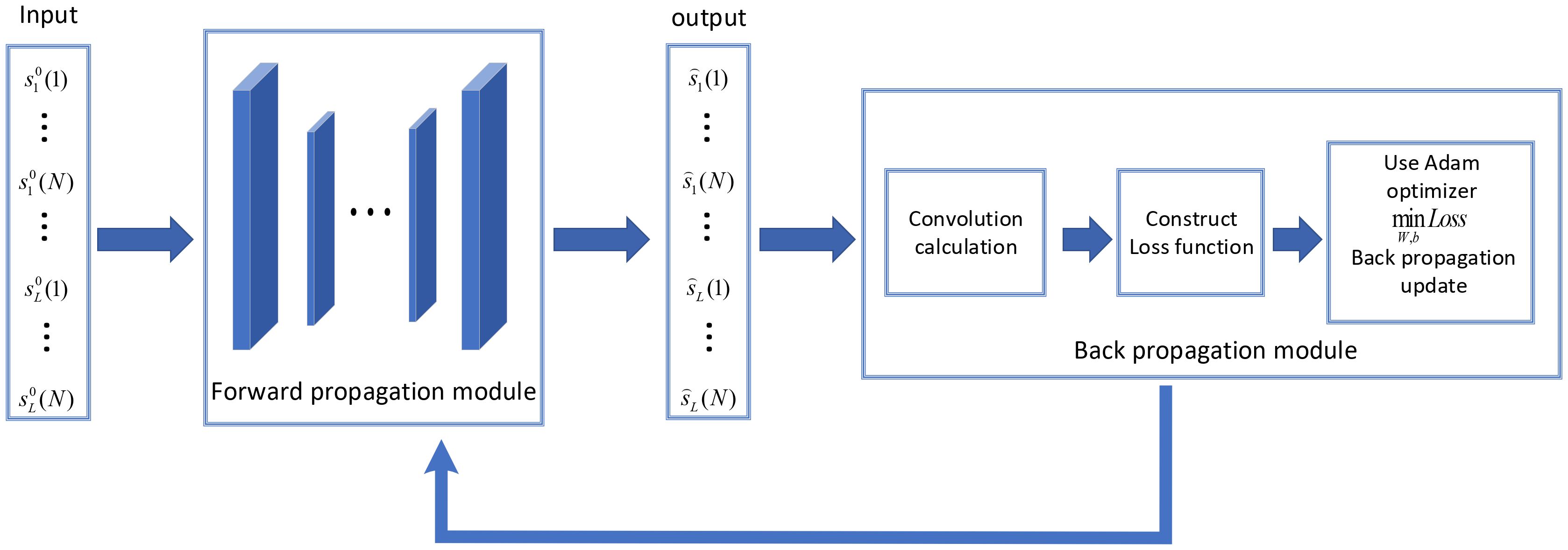
Figure 1. Optimization network structure diagram.

2.1 Input and output design

The input is the normalized phase sequence ${\mathit{s}}_1^0=[s_1^0(1),\dots s_1^0(N),\dots ,s_L^0(1),\dots ,s_L^0(N)]\in {ℝ}^{1\times (L\times N)}$, where $s_L^0(N)$ is the Nth phase of the Lth transmitted signal. The output of the forward propagation module is the phase sequence $\stackrel{⌢}{s}=[{\stackrel{⌢}{s}}_1(1),\dots ,{\stackrel{⌢}{s}}_1(N),\dots ,{\stackrel{⌢}{s}}_L(1),\dots ,{\stackrel{⌢}{s}}_L(N)]\in {ℝ}^{1\times (L\times N)}$. The designed normalized phase vector is reshaped into a phase matrix in the backpropagation module and then the phase matrix is converted into an ambiguity function matrix through convolution.

2.2 Forward propagation module

In the forward propagation module, the auto-encoder network is used to extract the features of the input, and the main features of the phase vector are retained in the process. Meanwhile, a certain number of hidden layers are designed in the auto-encoder network. The auto-encoder network has n fully connected layers with different numbers of neurons in each layer, and the Sigmoid function is used as the activation function.

As shown in Figure 2, the module can be divided into three parts: encoder, hidden layer, and decoder. The encoder consists of three layers and the number of neurons in each layer is specified as follows: Dim1 neurons in layer 1, Dim2 neurons in layer 2, and Dim3 neurons in layer 3, where Dim1=L × N, Dim2 = 0.5 × Dim1 + 2, Dim3 = 0.5 × Dim2. Similarly, the decoder also has three layers as illustrated in Figure 2, and the hidden layer has n-6 layers with Dim3 neurons in each layer. The signal features are better extracted through dimensionality reduction and expansion techniques.

Figure 2

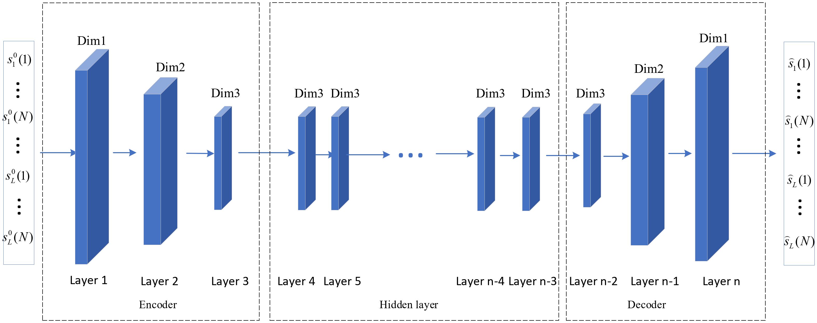
Figure 2. Network structure diagram of the forward propagation module.

2.3 Backpropagation module

In order to improve the adaptability of the signal in the actual channel, the influence of Doppler frequency shift should be considered in signal design (Li, 2007, 2009; Tian, 2013). Therefore, the ambiguity function is used to evaluate the signal, which can be expanded to the auto-ambiguity function(AAF) and the cross-ambiguity function (CAF) (Yang et al., 2024), The peak side-lobe level of the auto-ambiguity function at frequency shift $f_d\mathrm{=0}$ is denoted by APSL, and the peak side-lobe level of the auto-ambiguity function is denoted by AFPSL at non-zero Doppler frequency shift, and CFPSL denotes the peak side-lobe level of the cross-ambiguity function at non-zero Doppler frequency shift. Therefore, the evaluation criterion for the signal performance is as follows:

$$\underset{\Phi }{\min }{E}_1=\underset{\Phi }{\min }\max (APSL,{\lambda }_1·AFPSL,{\lambda }_2·CFPSL))$$

Where ${\lambda }_1$, ${\lambda }_2$ is the weight and the value range is [0,1].

The algorithm flowchart of the backpropagation module is shown in Figure 3, which consists of three parts: convolution computation, loss function calculation and backpropagation update. Firstly, the loss function is constructed with the ambiguity function matrix ${\widehat{Y}}^{\text{'}\text{'}}$ obtained by convolution computation. Subsequently, the Adam algorithm is used to minimize the loss function, and then the weights and offsets of the network in the forward propagation module are updated. Finally, a phase vector with low AFPSL and low CFPSL is generated when iteration stops.

Figure 3

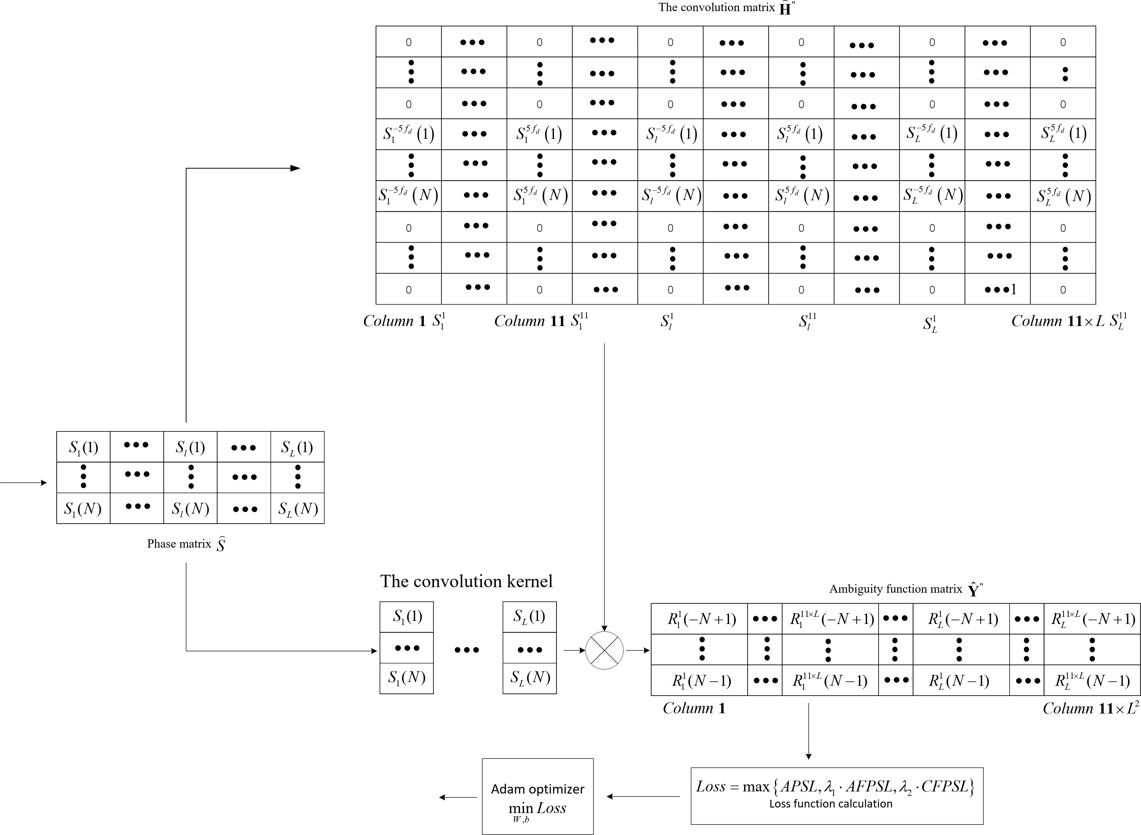
Figure 3. Algorithms flowchart of backpropagation module.

Before the convolution computation, the convolution kernel and convolution matrix are constructed, the convolution kernel is formed by concatenating the column phase vectors of L signals transversely and the convolution matrix ${\stackrel{⌢}{H}}^{″}$ is the expansion of the convolution kernel under different Doppler frequency shifts, taking signal 1 as an example. The expansion method is shown in Figure 4. The convolution kernel is padded with zero and expanded to different Doppler frequencies. Then, the extended matrix $\stackrel{⌢}{\text{H}}$′ of a single signal is obtained, and the frequency shift range is $[-5f_d,5f_d]$.

Figure 4

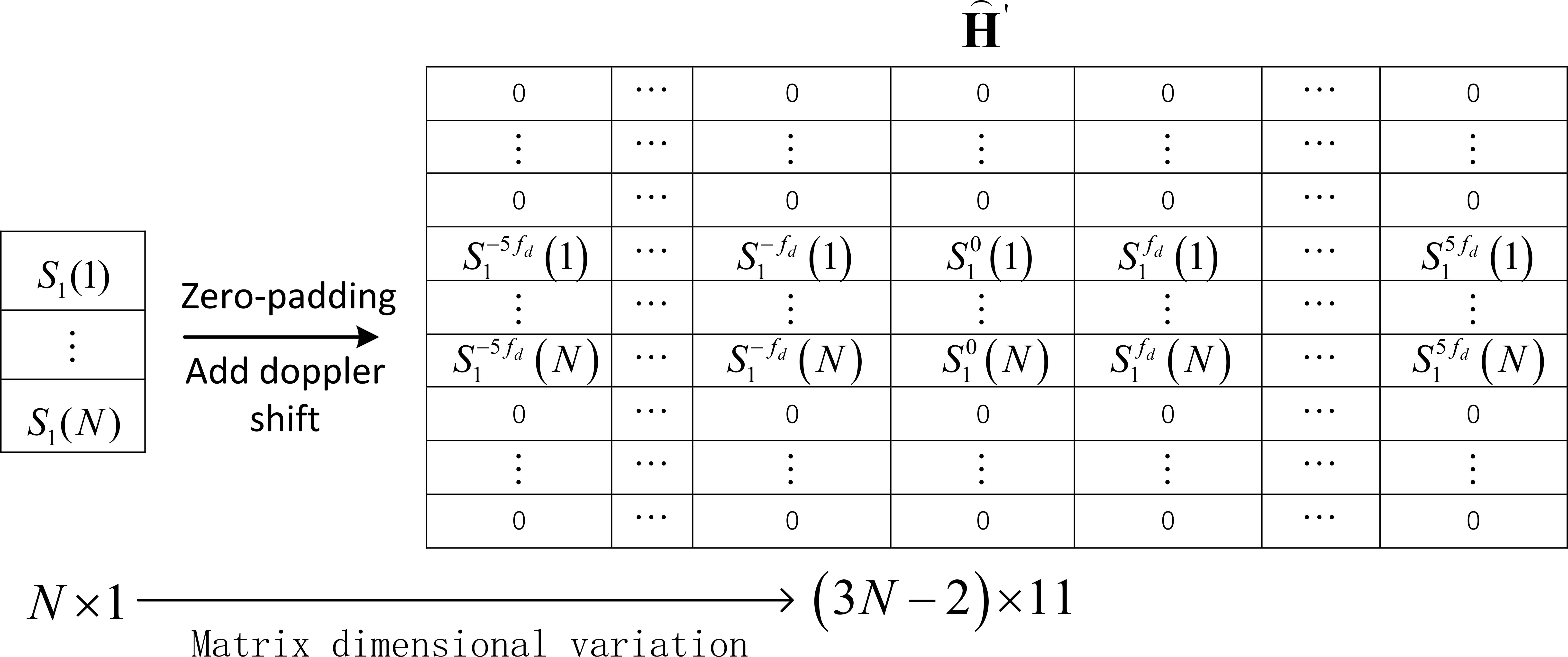
Figure 4. Schematic diagram of dimensional change of expansion matrix for single signal (eg:signal 1).

When there are four signals, the convolution matrix ${\stackrel{⌢}{H}}^{″}$ is formed by merging four extended matrices, and the dimension of each extended matrix $\stackrel{⌢}{\text{H}}$′ is $(3N-2)\times 11$, therefore, the dimension of the convolution matrix is $(3N-2)\times 44$.

As shown in Figure 5. Each signal is convolved with other signals at different Doppler shifts, including zero Doppler, to generate the matrix $Y^{\prime }$, which represents the convolution results between each signal and the convolution matrix ${\stackrel{⌢}{H}}^{″}$. Moreover, the ambiguity function matrix ${\widehat{Y}}^{\text{'}\text{'}}$ with a size of $(2N-1)\times 176$ is obtained by concatenating all the matrix $Y^{\prime }$ transversely. Due to the convolution computation process, the 6th, 61st, 116th, and 171st columns of ${\widehat{Y}}^{\text{'}\text{'}}$ are the auto-ambiguity function matrix at frequency shift $f_d=0$, and the APSL is obtained by calculating the maximum value of the auto-ambiguity function matrix after removing the Nth row, as the APSL is the maximum value after removing the main-lobe. The auto-ambiguity function matrix and the cross-ambiguity function matrix are formed by removing the above four columns of the matrix ${\widehat{Y}}^{\text{'}\text{'}}$, and AFPSL and CFPSL are obtained by calculating their maximum values, respectively.

Figure 5

Figure 5. Convolution computation process considering Doppler shift condition.

Subsequently, the Loss is calculated as follows:

$$Loss=\max \{APSL,{\lambda }_1·AFPSL,{\lambda }_2·CFPSL)\}$$

Finally, the loss function is minimized with the Adam optimizer and the network parameters are updated.

3 Optimization performance analysis

The CPU in the running environment is i9-8400, the GPU is GTX3080, and the RAM is 32G. The algorithm is processed with Python3.9.12 and Pytorch and runs on GPU.In this article, the influence of different network layers and the ambiguity function of the optimized signal are mainly analyzed.

3.1 Comparison under different numbers of network layers

In this section, the influence of different network layer numbers on the optimization is analyzed. The parameters are set as follows: the weight is ${\lambda }_1={\lambda }_2=1$, the initial learning rate is $\gamma =0.0005$, the number of iterations is E=30000, the number of signals is L=4, and the length of signal sequence is N=63. The number of network layers is [10,16,20,30,31,40,44,50,60], respectively, and the results shown in Figure 6 are obtained. Subsequently, the above experiment is repeated with the sequence length changed. Finally, the results shown in Figure 7 are obtained.

Figure 6

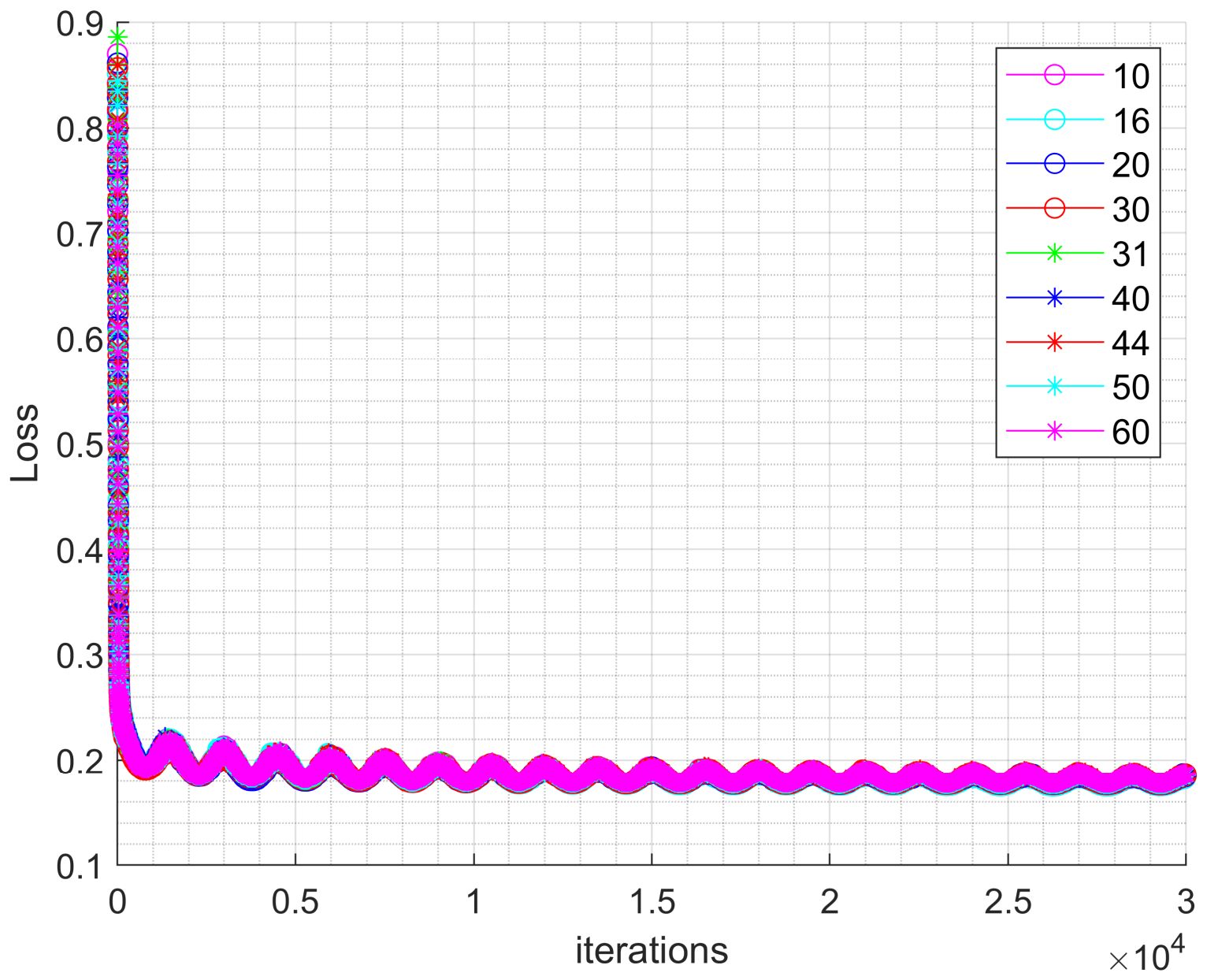
Figure 6. Comparison of loss values of different layers.

Figure 7

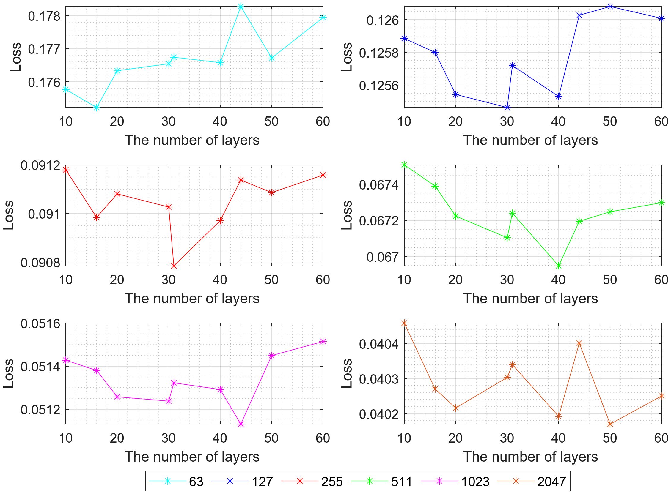
Figure 7. Comparison of loss values of different sequence lengths.

As illustrated in Figure 6 and Figure 7, For signals of a given sequence length, altering the number of network layers has little influence on the optimization performance. However, there is a layers number with optimal performance for each sequence length, and as the sequence length varies, the number of network layers with the best optimization performance also changes significantly, as shown in Figure 8.

Figure 8

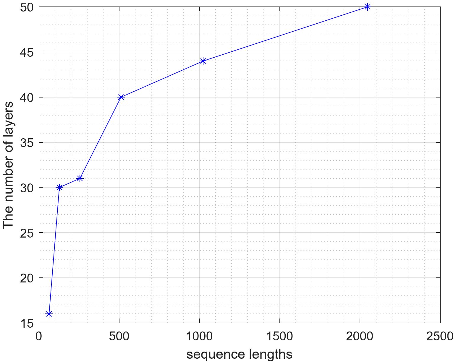
Figure 8. Relationships of layers number and sequence length under optimal optimizing performance.

3.2 Ambiguity function analysis under the same sequence length

The signal length is set to N=63 and the number of signals is L=4, the number of iterations is E=100000, the initial learning rate is $\gamma =0.0005$, and the weight is ${\lambda }_1={\lambda }_2=1$, the ambiguity function of m-sequence, GA algorithm, CON algorithm, and AON algorithm are compared and shown in Figure 9.

Figure 9

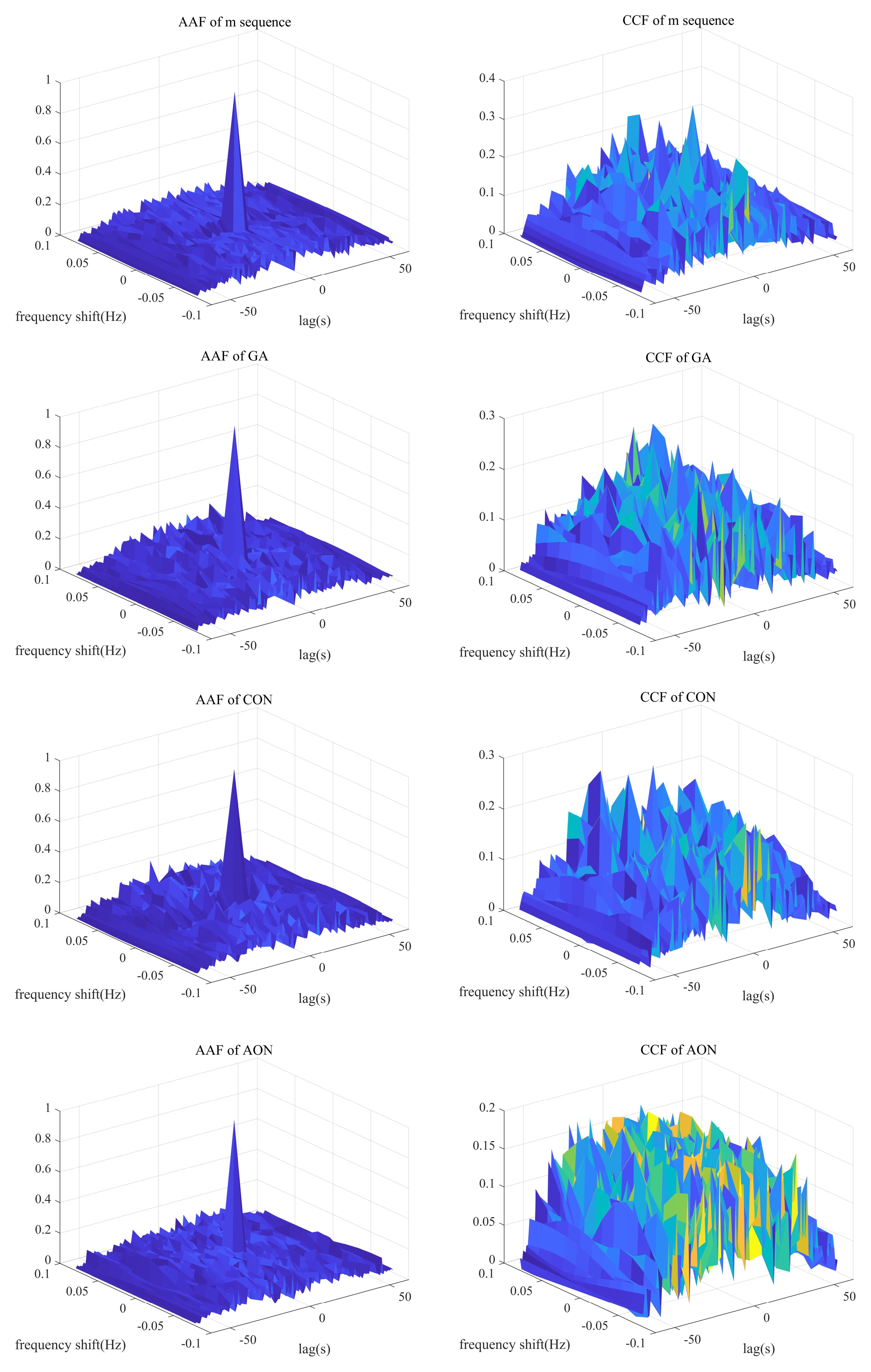
Figure 9. Auto-ambiguity function plots of different algorithms.

Figure 9 shows the auto-ambiguity and cross-ambiguity function diagram of the four algorithms, respectively.

The ambiguity function graph sections of signals generated by the four algorithms are analyzed to provide a clearer comparison of the four algorithms, which means the range ambiguity of signals are compared.

Figure 10 depicts the sections of the auto-ambiguity function and the cross-ambiguity function for the four algorithms, respectively. The APSL, AFPSL and CFPSL of the m-sequence are -17.9dB, -14.1dB and -10.5dB, respectively. The APSL, AFPSL and CFPSL for GA are -13.1dB, -10.2dB and -10.9dB, respectively. The APSL, AFPSL and CFPSL for CON are -20.6dB, -9.3dB and -11.2dB, respectively. Subsequently, It can be seen that the APSL, AFPSL and CFPSL of the proposed algorithm are all -15.1dB. Therefore, as the sequence length is set to N=63, the AFPSL of AON is 1 dB lower than that of the m-sequence, 4.9dB lower than that of GA and 5.8 dB lower than that of CON, additionally, the CFPSL of AON is 4.6 dB lower than that of the m-sequence, 4.2dB lower than that of GA and 3.9 dB lower than that of CON.

Figure 10

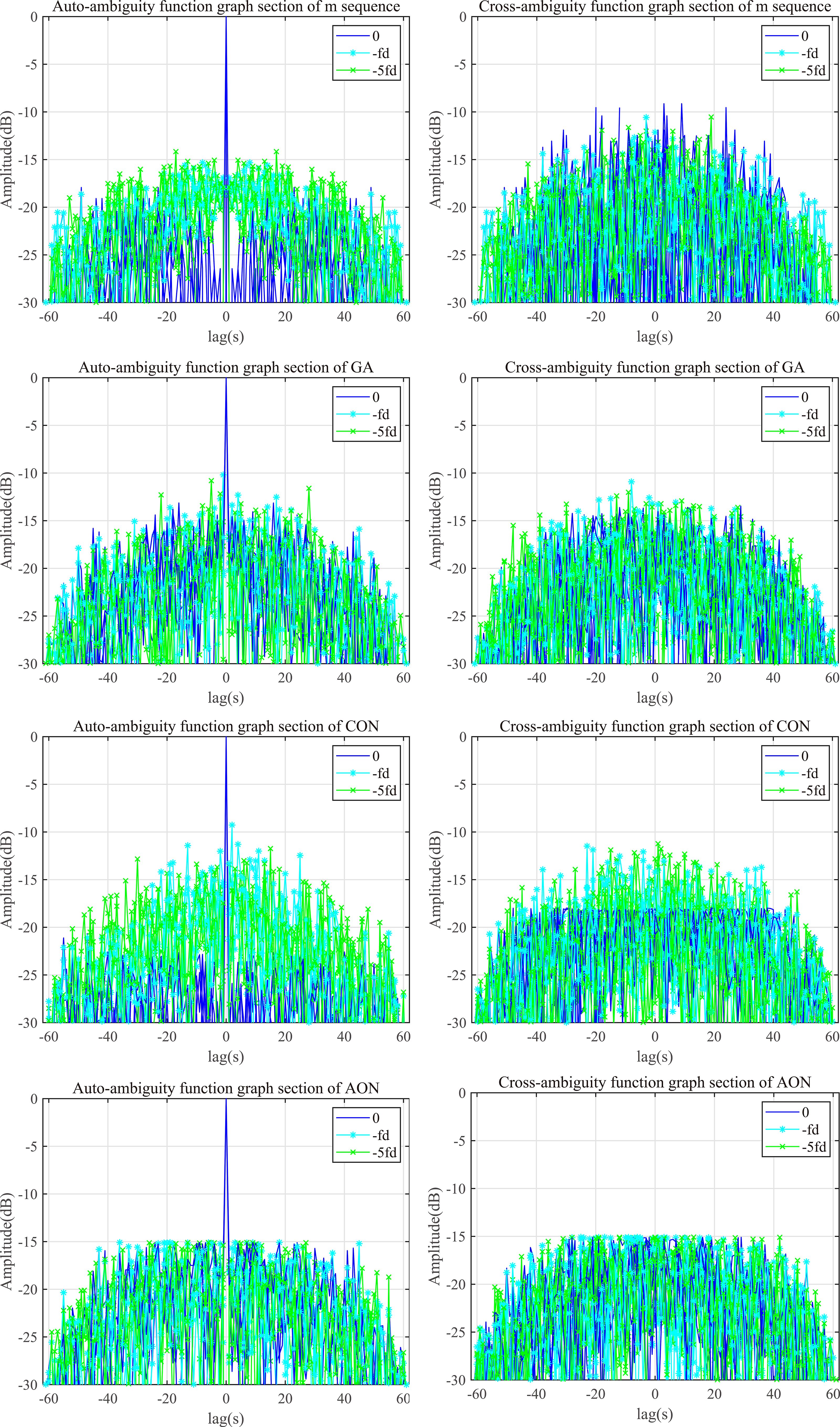
Figure 10. Ambiguty function diagram graph sections of different algorithms.

3.3 Ambiguity function analysis under different sequence lengths

The ambiguity functions of the proposed algorithm, GA algorithm, CON algorithm and M-sequence are compared under different sequence lengths. Signal number are set to L=4 and the sequence lengths are set to [63,127,255,511,1023,2047], the initial learning rate and iteration number are $\gamma =0.0005$ and E=100,000, respectively, the weights are ${\lambda }_1={\lambda }_2=1$. The comparison of APSL, AFPSL and CFPSL of each algorithm is shown in Figure 11, and the specific values are shown in Table 1 in dB.

Figure 11

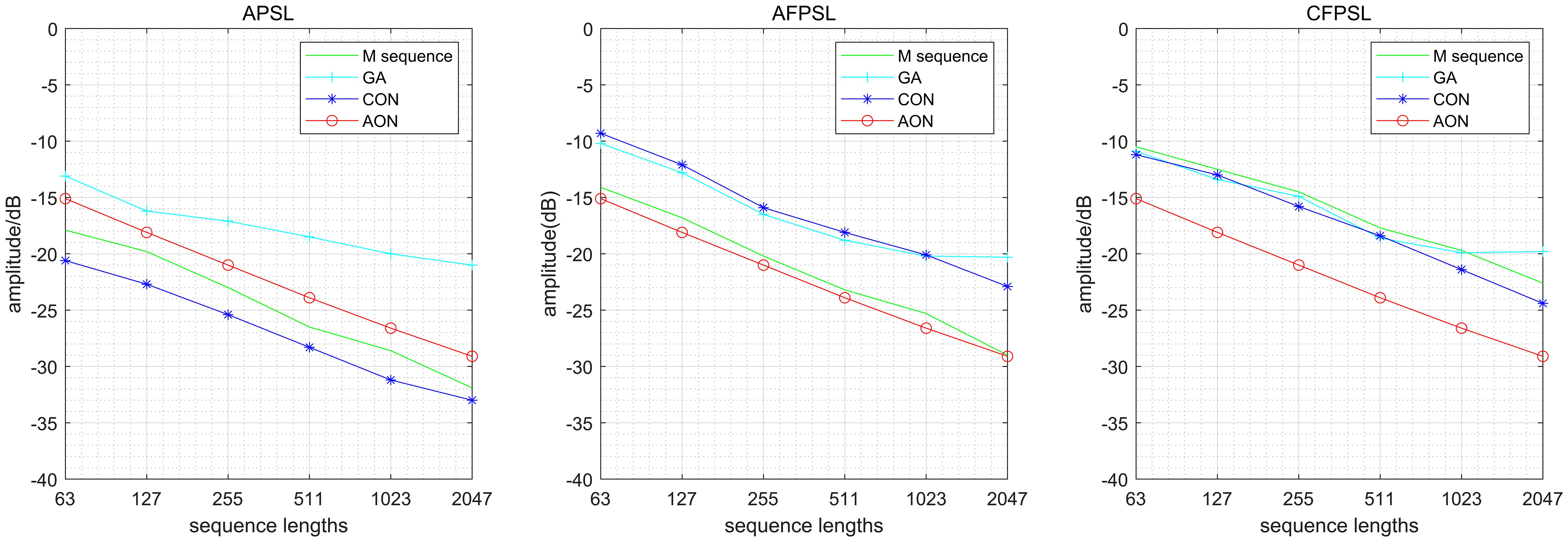
Figure 11. Comparison of APSL,AFPSL and CFPSL of different algorithms.

Table 1

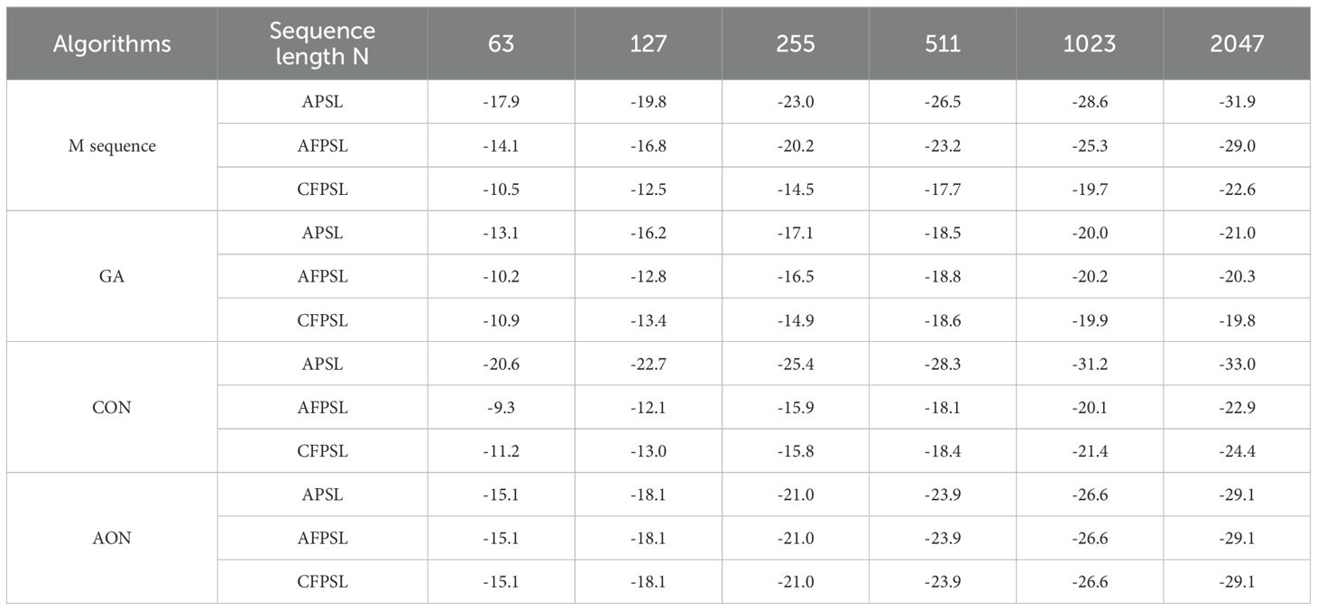
Table 1. Comparison of APSL, AFPSL and CFPSL of different algorithms.

As shown in Figure 11, the AFPSL and CFPSL of AON are lower than those of M-sequence and CON under Doppler frequency shift, while the APSL is higher than that of M-sequence and CON and lower than that of GA algorithm. According to Table 1, under different sequence lengths, The AFPSL of AON is 0.1dB to 1.3dB lower than that of M-sequence, 4.5 dB to 8.8 dB lower than that of GA algorithm and 5.1 dB to 6.5 dB lower than that of CON. Additionally, the CFPSL of AON is 4.6 dB to 6.9 dB lower than that of M-sequence, 4.2dB to 9.3dB lower than that of GA algorithm and 3.9 dB to 5.5dB lower than that of CON. Therefore, the performance of existing methods will be significantly reduced under Doppler frequency shift, which will probably lead to weak targets being masked by the side-lobes. Nevertheless, AON is capable of remaining a constant low side-lobe level under Doppler frequency shift.

3.4 Ambiguity function analysis under different sequence lengths

In this section, the optimization performance of AON, CON, GA algorithm and M-sequence is compared while L signals are transmitted simultaneously. Set the number of signals to L=4, the length of sequence to N=63, the learning rate of Adam to $\gamma$=0.0005, the number of iterations to E=100000, and the weight to ${\lambda }_1={\lambda }_2=1$.

It can be seen from Figure 12 that the AFPSL of AON is -5.6dB, the AFPSL of CON is -4.1dB, the AFPSL of GA is -5.4dB and the AFPSL of M sequence is -5.1dB. The AFPSL of AON is 0.5dB lower than that of M-sequence, 0.2dB lower than that of GA algorithm and 1.5dB lower than that of CON. This is because the cross-correlation performance will play a more critical role while L signals are transmitted at the same time.

Figure 12

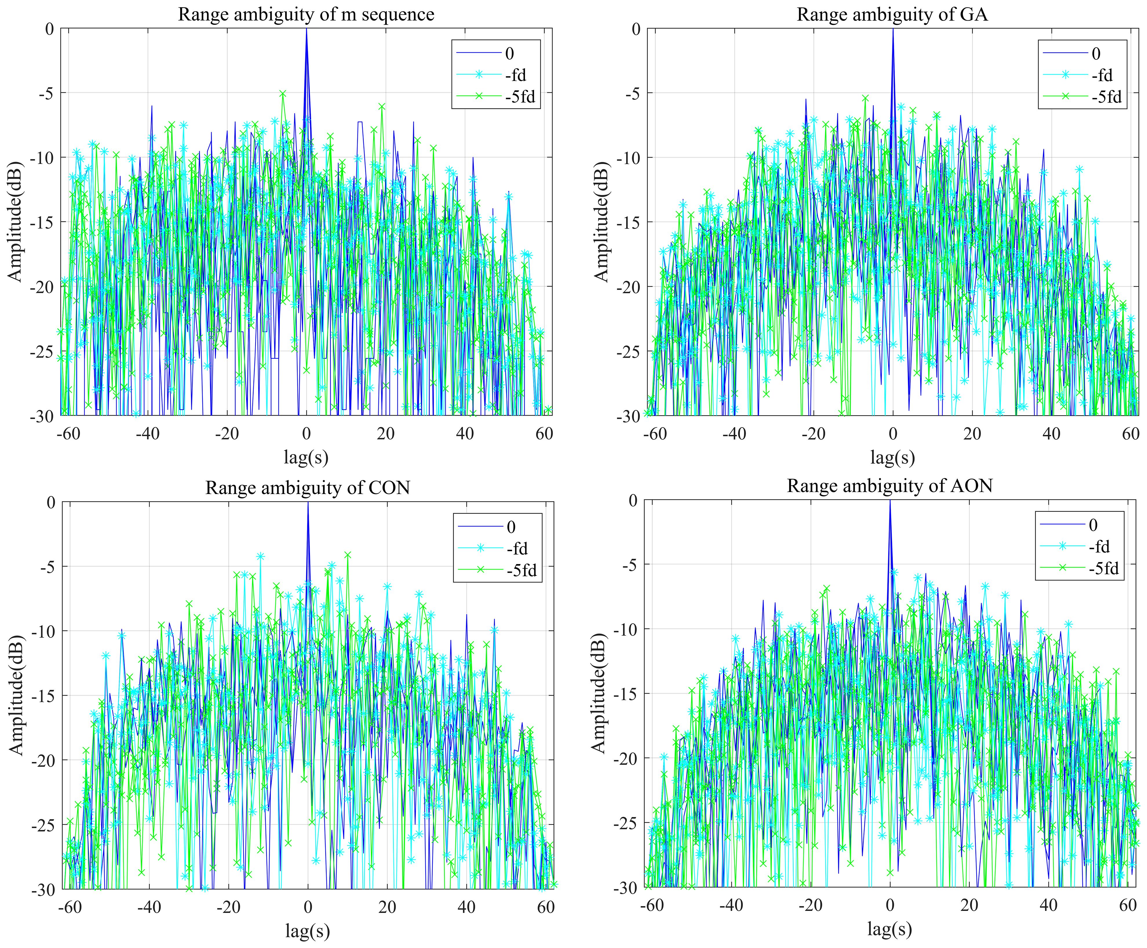
Figure 12. Auto-ambiguty function diagram graph cut for different algorithms in mixed signals.

When the sequence lengths are N=[63, 127, 255, 511, 1023,2047], the AFPSL of the above four algorithms is shown in Figure 13, and the specific values are shown in Table 2 in dB.

Figure 13

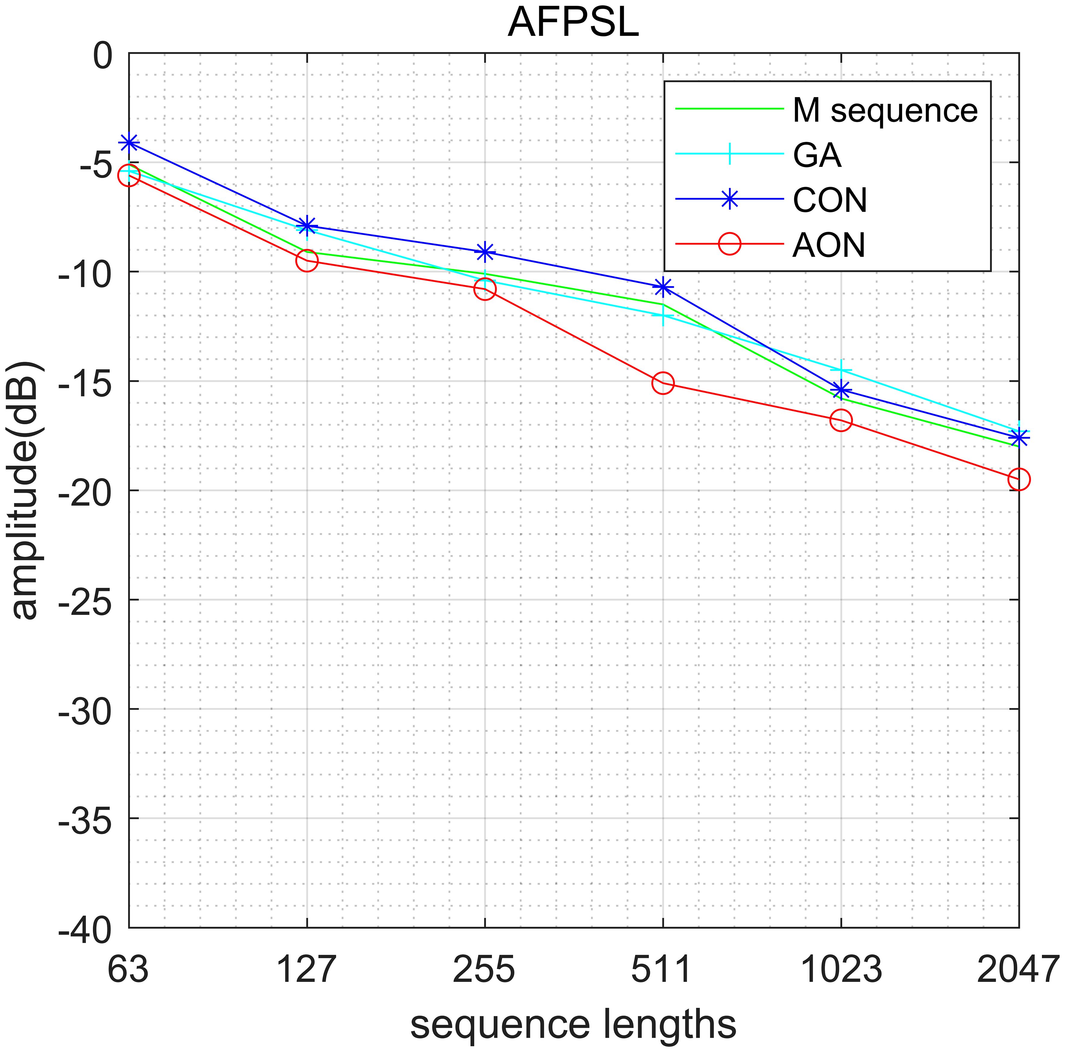
Figure 13. Comparison of AFPSL of different algorithms in the case of mixed signals.

Table 2

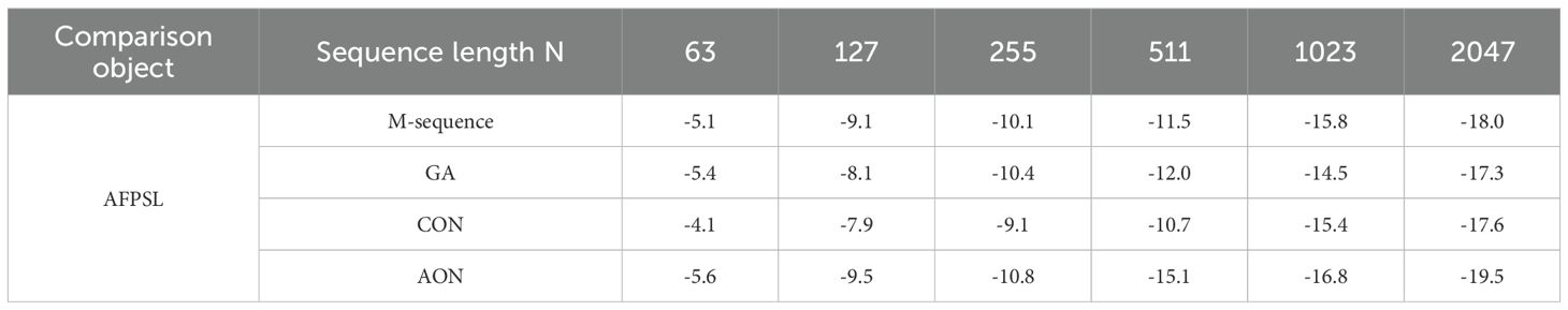
Table 2. Comparison of AFPSL of different algorithms in the case of mixed signals.

According to Figure 13, the AFPSL of AON is 0.4-3.6dB lower than that of M-sequence under different sequence lengths, 0.2-3.1dB lower than that of GA algorithm and 1.4-4.4dB lower than that of CON, which means that AON also has good performance under mixed signals.

3.5 Time complexity analysis

In this section, the time complexity of different algorithms is compared, the sequence lengths are set to [63,127,255,511,1023], the iterations of CON and AON are all 30000, the iteration of GA is 6000, the results are shown in Table 3.

From Table 3, while the runtime of AON is lower than that of GA, it can produce signals with lower side-lobe level under Doppler frequency shift. Besides, the optimization time of AON and CON are similar when the sequence length is low, but as the sequence length increases, the optimization time of AON is relatively long. This is because the network dimension of AON changes with the input size to better adapt to different signal lengths while the network dimension of CON remains unchanged.

Table 3

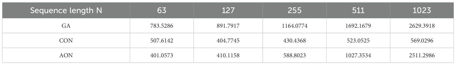
Table 3. Time(s) complexity analysis.

4 Summary

An orthogonal transmitted signal design method named AON is proposed in this paper, and the neuron numbers in different layers of AON are adjusted according to different sequence lengths. The signal design under Doppler frequency shift is mainly considered in this paper. This method can better extract the signal features based on auto-encoder, which leads to superior performance, and the weights and offsets of the forward propagation module are updated in the process by using the Adam optimizer, the learning rate of the Adam optimizer is dynamically adjusted through the CosineAnnealingLR method. Numerical results show that the proposed method can reduce both the AFPSL and CFPSL of signals, which means that signals generated by AON have better performance under Doppler frequency shift compared to existing methods.

Data availability statement

The original contributions presented in the study are included in the article/supplementary material, further inquiries can be directed to Sen Zhang, MTEwOTA0MTA3MEBudWUuZWR1LmNu.

Author contributions

BL: Writing – original draft, Formal analysis, Visualization. MW: Writing – original draft, Formal analysis, Visualization. SZ: Methodology, Supervision, Writing – review & editing, Validation, Conceptualization.

Funding

The author(s) declare financial support was received for the research and/or publication of this article. The study was funded by National Key Research and Development Program of China(JMRH-2024-0007-05).

Conflict of interest

The authors declare that the research was conducted in the absence of any commercial or financial relationships that could be construed as a potential conflict of interest.

Generative AI statement

The author(s) declare that no Generative AI was used in the creation of this manuscript.

Any alternative text (alt text) provided alongside figures in this article has been generated by Frontiers with the support of artificial intelligence and reasonable efforts have been made to ensure accuracy, including review by the authors wherever possible. If you identify any issues, please contact us.

Publisher’s note

All claims expressed in this article are solely those of the authors and do not necessarily represent those of their affiliated organizations, or those of the publisher, the editors and the reviewers. Any product that may be evaluated in this article, or claim that may be made by its manufacturer, is not guaranteed or endorsed by the publisher.

References

Cheng Z., Han C., Liao B., He Z., and Li J. (2018). Communication-aware waveform design for MIMO radar with good transmit beampattern. IEEE Trans. Signal Process. 66, 5549–5562. doi: 10.1109/TSP.2018.2868042

Crossref Full Text | Google Scholar

He K., Zhang X., Ren S., and Sun J. (2016). “Deep residual learning for image recognition,” in 2016 IEEE Conference on Computer Vision and Pattern Recognition (CVPR) (New York: IEEE Computer Society), 770–778. doi: 10.1109/CVPR.2016.90

Crossref Full Text | Google Scholar

Hu J., Wei Z., Li Y., Li H., and Wu J. (2021). Designing unimodular waveform(s) for MIMO radar by deep learning method. IEEE Trans. Aerosp. Electron. Syst. 57, 1184–1196. doi: 10.1109/TAES.2020.3037406

Crossref Full Text | Google Scholar

Huang C.-W., Chen L.-F., and Su B. (2023). Waveform design for optimal PSL under spectral and unimodular constraints via alternating minimization. IEEE Trans. Signal Process. 71, 2518–2531. doi: 10.1109/TSP.2023.3291454

Crossref Full Text | Google Scholar

JayaSree M. and Rao L. K. (2022). “A deep insight into deep learning architectures, algorithms and applications,” in Proceedings of the International Conference on Electronics and Renewable Systems, ICEARS 2022 (New York: Institute of Electrical and Electronics Engineers Inc). 1134–1142. doi: 10.1109/ICEARS53579.2022.9752225

Crossref Full Text | Google Scholar

Kingma D. P. and Ba J. (2015). “Adam: a method for stochastic optimization,” in ICLR 2015 - Conference Track Proceedings, 2015 (San Diego, CA, United states: International Conference on Learning Representations).

Google Scholar

Krizhevsky A., Sutskever I., and Hinton G. E. (2017). ImageNet classification with deep convolutional neural networks. Commun. ACM 60, 84–90. doi: 10.1145/3065386

Crossref Full Text | Google Scholar

Li G. (2007). Research of phase-coherent communications and adaptive equalization for UWAChannels (Xian: Northwesten polytechnical University).

Google Scholar

Li P. (2009). Study of the doppler effects on pulse compression radar and the doppler compensation (Wuhan: Huazhong University of Science and Technology).

Google Scholar

Liu B., He Z., Zeng J., and Liu B. (2006). “Polyphase orthogonal code design for MIMO radar systems,” in CIE International Conference of Radar Proceedings (New York: Institute of Electrical and Electronics Engineers Inc), 1–4. doi: 10.1109/ICR.2006.343409

Crossref Full Text | Google Scholar

Liu T., Sun J., Wang G., Du X., and Hu W. (2023). Designing low side-lobe level-phase coded waveforms for MIMO radar using P-norm optimization. IEEE Trans. Aerosp. Electron. Syst. 59, 3797–3810. doi: 10.1109/TAES.2022.3232310

Crossref Full Text | Google Scholar

Minsky M. and Papert S. A. (2017). Perceptrons: an introduction to computational geometry (Cambridge: MIT Press).

Google Scholar

Pu Z. (2020). Design and performance analysis of orthogonal waveform for MIMO radar (Nanjing: Southeast University). doi: 10.27014/d.cnki.gdnau.2019.002024

Crossref Full Text | Google Scholar

Tian X. (2013). Research on doppler characteristics and a compensation method for biphase coded signal. Electronic Sci. Tech 26, 31–33. doi: 10.16180/j.cnki.issn1007-7820.2013.09.022

Crossref Full Text | Google Scholar

Wang J. and Wang Y. (2021). Designing unimodular sequences with optimized auto/cross-correlation properties via consensus-ADMM/PDMM approaches. IEEE Trans. Signal Process. 69, 2987–2999. doi: 10.1109/TSP.2021.3079819

Crossref Full Text | Google Scholar

Wei Z. (2022). Research on MIMO radar waveform optimization theory and algorithm based on deep learning (ChengDu: University of electronic science and technology of China). doi: 10.27005/d.cnki.gdzku.2021.004358

Crossref Full Text | Google Scholar

Yang C., Yang W., Qiu X., Jiang W., and Liu Y. (2024). “Design of high doppler tolerance orthogonal sequence set via ambiguity functions shaping,” in Proceedings of 2024 9th International Conference on Frontiers of Signal Processing (New York: Institute of Electrical and Electronics Engineers Inc), 184–188. doi: 10.1109/ICFSP62546.2024.10785426

Crossref Full Text | Google Scholar

Zhang W., Hu J., Wei Z., Ma H., Yu X., and Li H. (2020). Constant modulus waveform design for MIMO radar transmit beampattern with residual network. Signal Process. 177, 107735. doi: 10.1016/j.sigpro.2020.107735

Crossref Full Text | Google Scholar

Zhou G., Zhu X., Song C., Fan Y., Zhu H., Ma X., et al. (2018). “Deep interest network for click-through rate prediction,” in Proceedings of the ACM SIGKDD International Conference on Knowledge Discovery and Data Mining (New York: Assoc Computing Machinery), 1059–1068. doi: 10.1145/3219819.3219823

Crossref Full Text | Google Scholar