The Finnish Ice Service, its sea-ice monitoring of the Baltic Sea and operational concept

The Finnish Ice Service is part of the Finnish Meteorological Institute (FMI). Based on the mandate in the Finnish legislation, it provides information on the ice conditions in the Baltic Sea. This paper introduces the methods used by the Finnish Ice Service, data sources, products, services, datasets, and supporting Baltic Sea ice remote sensing and geophysics research conducted at FMI. The predecessor of the Finnish Ice Service started its operational ice charting in 1915 to provide ice information for the winter navigation. To this day, the main users still are the winter navigation authorities, including the icebreaker fleet and management, as well as the shipping community, scientists and general public. The focus area is the Baltic Sea. Typically, the service operates from mid-October to the end of May, providing up-to-date sea-ice information in several products and formats. The prevailing ice situation is described in ice charts, ice reports and ice codes, which are based on a range of different observation sources like satellite images, predominantly from synthetic aperture radars, and surface observations from both icebreakers and coastal observers. The Finnish Ice Service has long sea ice observation timeseries and archives of manually analysed ice charts. To help users and customers optimize their operations in ice infested waters, the Finnish Ice Service provides numerical and manual sea ice forecasts with various forecast lengths. The Finnish Ice Service processes and disseminates satellite data and also provides advisory and consultant services to users. As FMI is committed to the open data policy, the main ice service products are provided free of charge. A number of products are also available through the Copernicus Marine Service (CMS).

1 Introduction

Sea ice has always been intriguing and interesting for a lot of people and for many reasons. To know its structure and physics are scientifically important, but it also has a major effect on the transport at sea. In the seasonally ice-covered sea areas, like the Baltic Sea, the ice conditions must be taken into account in shipping and other travelling (Figure 1). Understanding sea ice and its behaviour, and translating that understanding into supportive services for shipping, was early identified as a key topic for the countries on both sides of the northern Baltic Sea (WNRB, 1972). Continuous shipping also during wintertime has been considered a vital component for maintaining a competitive national economy (MINTC, 2014). The Finnish Ice Service has been established to support and facilitate this wintertime activity.

Figure 1

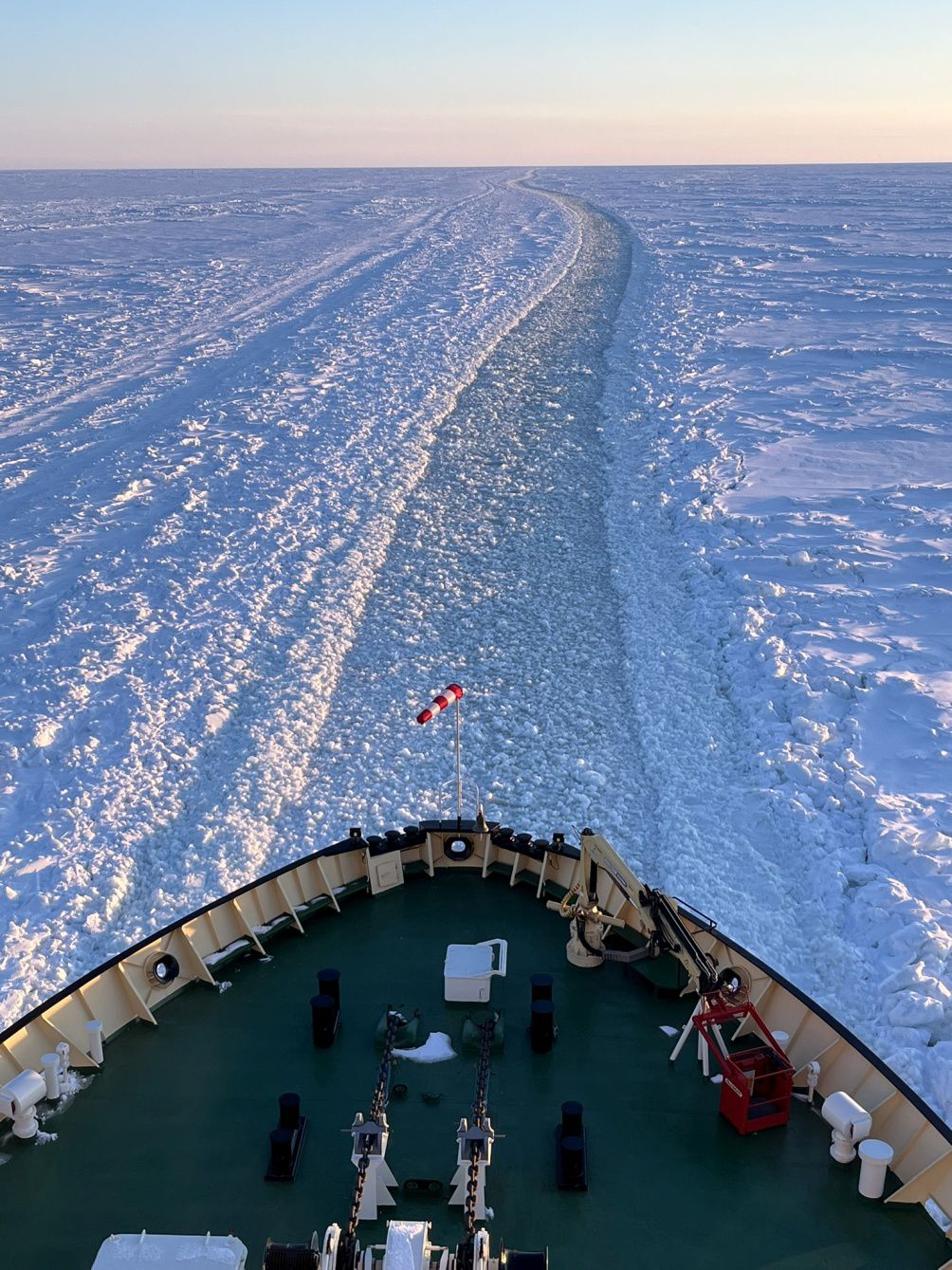
Figure 1. Sea ice field and ship track in the Bay of Bothnia as seen from the bridge of the Finnish icebreaker Urho (photo: Jarkko Toivola).

1.1 History of the Finnish Ice Service

The Baltic Sea has always been an important sailing route and in the 19^th century there was a rising interest in extending the navigational season also during winter. For this purpose, many different ways of observing and exchanging information on ice conditions were created. In 1846, the Finnish Society of Sciences and Letters began to collect ice observations from the coastal sea areas. Since then, the work has increasingly been carried out to favour economic interests. In 1890, Finland got its first icebreaker called ‘Murtaja´ (Ramsay, 1949).

At the very end of the 19th century, the ice observation network was made operational. Ice charts were drawn at eight lighthouses along the Finnish coast. The work was supervised by the Finnish Society of Sciences and Letters. However, the data was collected with a delay. The World War I changed the situation. The Russian Imperial Navy quickly needed reliable ice data for its strategic planning and merchant ships also needed better and more real-time sea ice information. The Imperial Navy ordered the Finnish Society of Science and Letters to make real-time ice charts. The Finnish Society of Science and Letters began to renew its observation routines, and since March 1915, ice charts were drawn weekly (Granqvist, 1926).

The Finnish Institute of Marine Research (FIMR) began its operation on the 1^st of January 1919 with the task of studying and monitoring the sea areas around Finland. At the same time, the existing ice monitoring duties were transferred to FIMR, where the ice service now was an essential part of the institute’s functions. The first ice chart published by the institute was on the 17^th January 1919 (Witting, 1920). The Finnish Ice Service was part of FIMR until it was disbanded 31.12.2008. Since then, the Finnish Ice Service, along with ice research and physical oceanography, has been part of FMI. Today the Ice Service is part of FMI’s operational duty functions. The Institute’s main duties are to observe and research the atmosphere, near space, and the seas, and to provide information and services for public safety, businesses, and citizens.

An in-depth historical review of the Ice Service’s first 75 years has been published by Seinä et al. (1997).

1.2 The Baltic Sea

The Baltic Sea is a semi-enclosed brackish sea water basin in Northern Europe. The ice cover in the Baltic Sea usually begins to form in November and has its largest extent between January and March (Leppäranta, 1984). The normal ice break-up starts in April and the ice melts completely by the beginning of June. The maximum annual extent of ice cover in the Baltic Sea has varied from 37–000 km² to 420–000 km² (which is the whole Baltic Sea coverage). As longest, the ice season may be up to 220 days in the northern Bay of Bothnia. Figure 2 shows time series of maximum ice extent in 1971-2024.

Figure 2

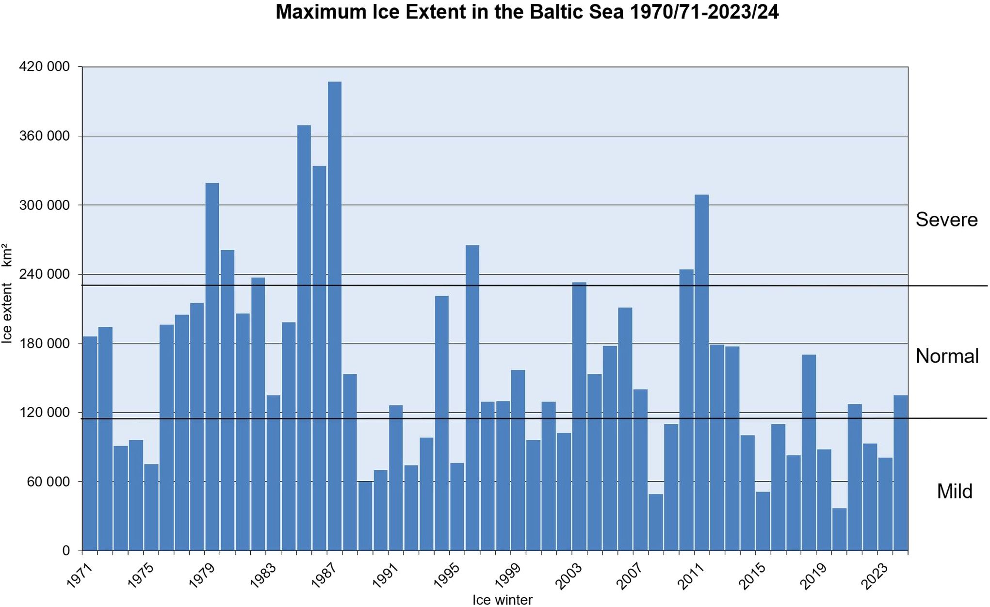
Figure 2. Maximum ice extent of the Baltic Sea 1970/71 - 2023/24, including the ice winter severeness limits.

The ice in the Baltic Sea occurs as landfast ice and drift ice. Landfast ice occurs in the coastal and archipelago areas. Drift ice has a dynamic nature due to forcing by winds and currents. The motion of drift ice results in an uneven and broken ice field with distinct floes up to several kilometres in diameter, leads and cracks, brash ice barriers, rafted ice and ice ridges. In the Bay of Bothnia, the annual maximum level ice thickness is typically 0.65–0.80 m, and it reaches 0.3–0.5 m even in mild winters (Seinä and Peltola, 1991; Vihma and Haapala, 2009). The measured all time maximum is around 1.2 m. In the Southern Baltic Sea, the coastal areas of Germany and Poland and the Danish Straits, the annual maximum level ice thickness seldom exceeds 0.5 m (Leppäranta and Hakala, 1992). The thickness of ice ridges, calculated as the sail height plus keel depth, is typically 5 to 15 m (Leppäranta and Hakala, 1992). The salinity of the Baltic Sea ice is typically from 0.2 to 2‰ depending on the location, time and weather (Hallikainen, 1992).

1.3 Finnish Ice Service today

The Finnish Ice Service operates at the FMI under the Ministry of Transport and Communications, alongside other maritime agencies. The service is part of the Oceanographic Services group, within the Weather and Safety Centre, working side by side with the operational weather forecasters, see Figure 3. The Ice Service staff currently consists of six junior and senior sea ice analysts, located in the FMI main office in Helsinki.

Figure 3

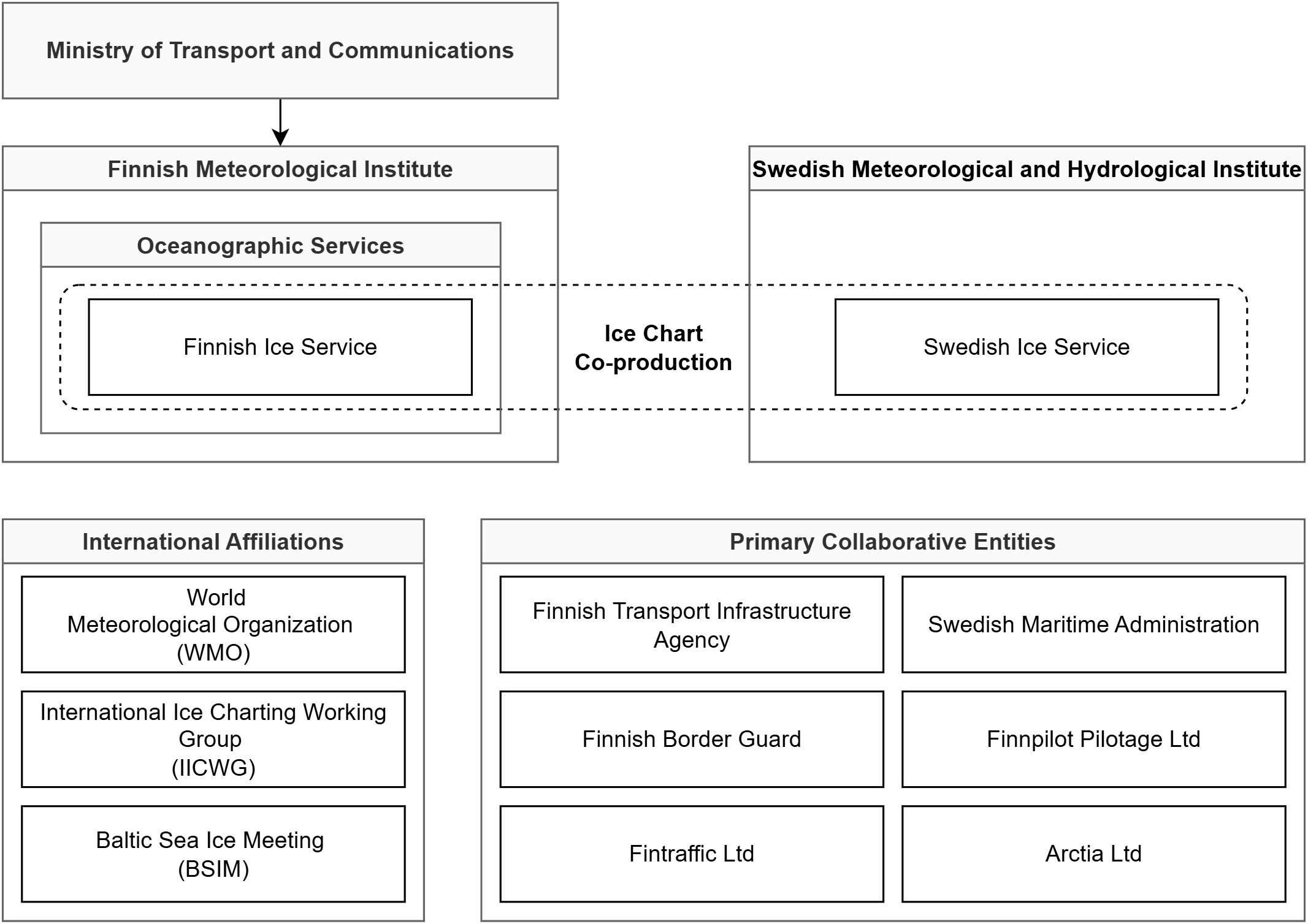
Figure 3. Organizational chart of the Finnish Ice Service and its most important connections.

Nowadays approximately 95% of Finland’s international trade is transported by sea (Tulli, 2024). Finland and Estonia are the only countries in the world where all mainland harbours freeze during normal winters. Operating effectively and safely in ice conditions is crucial for year-round commercial shipping and supply security.

Still today, the main purpose of the Ice Service is to provide ice information for the support of winter navigation. Wintertime ship navigation and icebreaker operations in the Baltic Sea rely heavily on this information, provided by national Ice Services. The other users are researchers and citizens interested in ice conditions. The most important source of sea ice information is provided by satellite images. Other sources include sea ice model data and in-situ observations. The most important sea ice parameters comprise the location of the sea ice edge, sea ice and snow thickness, degree of deformation and ice concentration (Berglund and Eriksson, 2015).

The daily ice chart is the main product of the Ice Service, but the work consists of several other duties too. The Finnish Ice Service provides ice information as text and in numeral formats, makes ice forecasts, gives consultancy services and answers questions from the public and media.

The Finnish Ice Service is closely co-operating with the Ice Service at the Swedish Meteorological and Hydrographical Institute (SMHI). Since the winter 2017/18 the ice chart has been produced together, on a week-to-week basis.

The Finnish Ice Service is part of the international network of ice experts and the ice expert community of the Baltic Sea. It is a founding member of the International Ice Charting Working Group (IICWG) and the Baltic Sea Ice Meeting (BSIM) and an active member of the World Meteorological Organization (WMO).

2 Operational service

2.1 Description of the operational routines

The Finnish Ice Service starts operation in early October by monitoring the cooling of the sea surface water. Charts with analysed SST’s are produced bi-weekly, on Mondays and Thursdays. The start date has varied on the course of time, but in recent years it has been fixed to the start in mid-October. When the freezing starts and ice conditions become more challenging for the maritime traffic, the Finnish Transport Infrastructure Agency (FTIA) or the Swedish Maritime Administration (SMA) sends out their first icebreakers and issue national assistance restrictions for the ships. That triggers daily production of the ice charts, ice reports and ice codes along with the other ice service products and services, see Figure 4 for operational workflow. Typically, this happens in mid-December but may vary between late November and early January. During normal operation in mid-winter, ice charts are published daily seven days a week until the ice melt-up. The ice service is continued until the sea ice has practically melted from the northern Baltic Sea, typically mid-May [varying from early May to early June (FMI, 2025)]. The typical operation day starts when the ice analyst checks the weather observations and forecasts, the previous day’s ice conditions and the icebreaker and administration messages and announcements. Then the ice analyst goes through all available satellite images, which serve as a backbone for the sea-ice charting. The Synthetic Aperture Radar satellites (SAR), which are the main source of spatial information, are in a sun-synchronous polar orbit, meaning the acquisition happens early morning and early evening. The downlinking and processing take from 30 minutes up to a few hours, and images are available for the analyst in the morning, well before noon. Analysis of the ice situation is typically based on morning SAR images, but in lack of such, the previous evening’s SAR images or optical satellite images are used. The darkness and cloudiness frequently prohibit the use of optical satellites until March. The ice report is written before noon, and the assisting ice analyst translates it to Swedish and English and publishes it around noon. After this the ice chart is finalized. The ice chart contains information from the icebreaking administrations in both Finland and Sweden and is added to the chart along any additional comments from the stand-by institute. The ice chart is published in the afternoon around 2 pm. At the end of the day, the ice codes are generated and published.

Figure 4

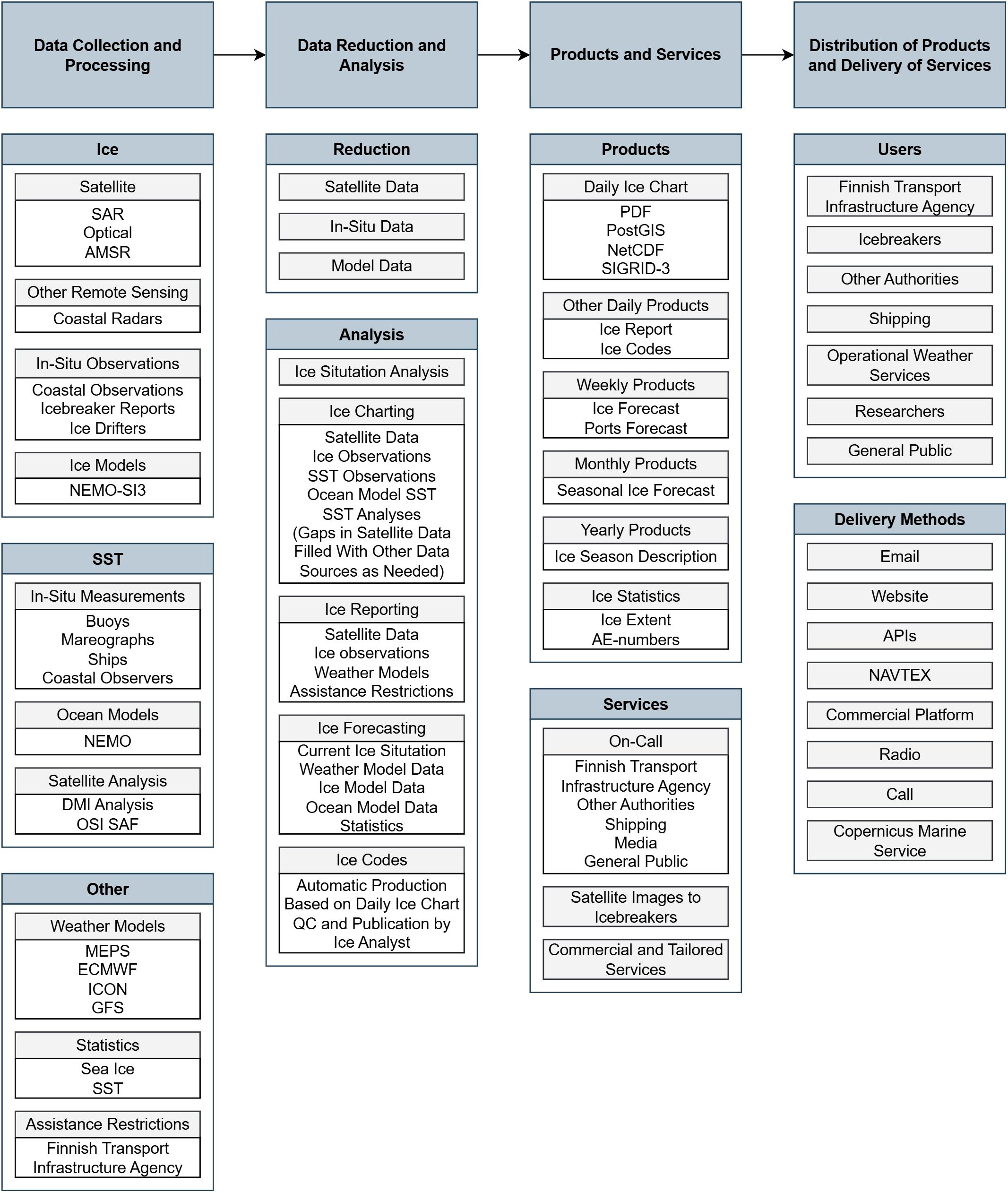
Figure 4. Operational workflow at the Finnish Ice Service.

At present, three ice experts are responsible for the ice information production. The duty work is conducted during office hours, also including weekends. In addition to the operational duties, the ice experts are responsible for various support tasks. These include ordering satellite images, managing the ice observation network and numerical processing of observation data, to mention a few. Since the operational duty is limited to office hours, it may not be possible to get answers to questions about satellite imagery on weekends or in the evenings. However, inquiries about the ice situation on weekends and often also in the evenings are answered, as the on-call phone is forwarded to the mobile phone of the ice expert on duty. The on-duty ice expert also responds to inquiries from the media.

The co-production with the Swedish Ice Service runs on a week-to-week basis, where one of the ice services is doing the analysis from Tuesday to Monday, and the other is in stand-by. Other products and services than ice charts are produced separately at each institute. Thus, when the FMI Ice Service is in standby mode, the SMHI Ice Service performs the actual ice charting, but a certain review of the ice condition is anyhow done at FMI in order to be able to issue ice reports and codes and serve any customers, the media or other users.

For the ice charting, commonly available GIS software are used. At the moment of writing, FMI is using ArcGIS10 with in-house developed plug-ins, co-developed with the SMHI ice service. FMI uses its own ice service tools and software, dedicated for generating and publishing ice reports and ice codes. The data formats are commonly used standard formats, such as pdf’s, shapefiles, png’s or plain text.

2.2 Winter navigation authorities

The operational winter navigation function can be seen as a consortium of the units of the different authorities that manage ice navigation to Finnish ports. The winter navigation is managed by the Finnish Traffic Infrastructure Agency and supported by the relevant actors at Fintraffic VTS (Vessel Traffic Service), the Border Guard, the pilotage company FINNPILOT and the FMI Ice Service. One of the most important elements of the winter navigation is the assistance provided by icebreakers and the associated assistance restriction system. The Ice Service contributes to the dissemination of this navigational information by including the restriction information in both the ice chart and the ice reports.

The Ice Service works closely with the icebreaking operation, and the on-duty ice analyst closely monitors the reports and ice observations from the icebreakers and pilots, using these to describe the ice situation. From icebreaker reports, it is possible to interpret many other details about the ice conditions than just specific ice observation information. For example, the trafficability and difficulty in a sea area can be interpreted if an icebreaker reports the need for towing vessels, which types of vessels manage without assistance and which not, or where vessels get stuck in the ice. Additional aid to the ice analysis can be retrieved from the icebreakers’ observations of the ice drift.

2.3 IBNet

The icebreaking operation uses an online information system called IBNet. It is jointly developed and operated by the Finnish Transport Infrastructure Agency and the Swedish Maritime Administration for coordination of the joint icebreaking operations by the two neighbouring countries. IBNet contains information about the weather, ice and traffic situation, and transmits the information between the different connected units (icebreakers, coordination centres, VTS etc.) (BIM, 2020). The Ice Services in both Finland and Sweden have access to the system in order to share information with the icebreaking parties.

In IBNet, the icebreakers report on the prevailing ice conditions in their respective operation areas. This reporting is done on a regular basis with several reports per day. The reporting form contains predefined fields for the most important sea ice parameters: ice concentration, thickness, degree of deformation, ice pressure, drift direction and speed, weather and a free text field for additional ice information.

FMI can also be considered a content producer for IBNet. The satellite data processed by FMI are uploaded to its data interface (WMS server), from where the IBNet server extracts them in an agreed format in near-real-time. Also weather observations, weather and ice forecasts and water level observations are visualized in IBNet. In the map user interface of IBNet, the icebreaking personnel can visualize all metocean products, including satellite imagery, in one view together with essential traffic and maritime information (AIS targets and tracks, fairway information etc.). The information provided by FMI via IBNet also serves pilots and VTS centres.

2.4 Commercial and tailored services

In addition to the daily ice monitoring, the FMI Ice Service also provides customized services like briefings, and special operational services. The Ice Service offers tailored products like weather and ice case studies, official statements and statistical ice studies and reports. The clients for these products are often entities involved in navigation, offshore construction or coastal engineering.

As the FMI operates a separate Customer Services unit, the Ice Service naturally works in close cooperation with the maritime sector of that unit, providing content and expertise to their services.

3 Input data sources

Like most ice services in the world, the FMI Ice Service also collects data from all available sources and compiles it in a number of different outputs, in particular in the form of an ice chart in vectorized form (polygons with several parameters) (WMO, 2021). The analysis is almost entirely based on manual interpretation made by ice analysis experts. The most important ice information sources are 1) satellite images, 2) icebreaker observations, 3) manual observations from coastal stations, 4) ice drifters and 5) numerical prediction models, in order of importance. The output formats are printable charts (PDF), NetCDF grids and the Shape-like SIGRID-3 format (although still in Beta phase).

3.1 Ice thickness and sea surface temperature observations

FMI has around 20 ice observation stations along the Finnish coast where fast ice thickness is measured manually by drilling a hole through the ice, see Figure 5 Observers are typically local people like fishermen, ice skaters, or border guards. If the ice situation doesn’t allow an observer to go on the ice, ice thickness can be visually estimated. The snow depth on ice is also measured. Measurements are done once a week and delivered to the Ice Service using an electronic form. The oldest observations were done in 1897. Most of the old observations are in paper form. Since 2016, observations have been collected in digital form. In addition to FMI’s own observation network, ice observations are obtained directly from icebreakers, as described above.

Figure 5

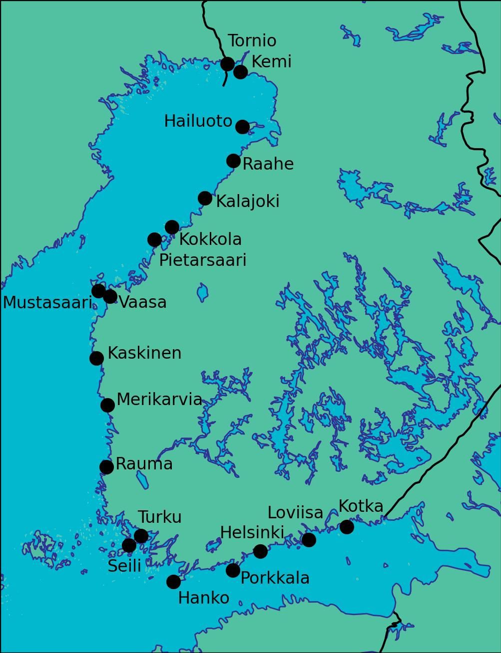
Figure 5. Locations of the FMI coastal ice observation stations active in the recent years. In some locations there are multiple measurement stations close by.

Sea Surface Temperature (SST) is measured by water level measurement stations, wave and temperature buoys, and fixed stations. In total, FMI has around 30 temperature measurement sites. The vast majority of buoys are lifted up for the winter. In addition, SST information is obtained from a few merchant ships travelling in the Baltic Sea with a Ferry Box or hull thermometer installed. Not all SST observations are obtained in real-time. The ice analysis takes into account up to two days old temperature observations. In addition to surface observations, temperature information is also collected from satellite analysis products, like OSI SAF products offered by Eumetsat, and from numerical oceanographic models.

3.2 Satellite data

Remote sea-ice monitoring was done by means of aerial reconnaissance from 1934 through an agreement with the Navy and the Coast Guard. In the 1940’s, aerial reconnaissance was already a regular help for the ice monitoring and for the winter navigation. Later, the airplanes were replaced by helicopters operated from icebreakers. With the introduction of satellite imaging in the late 1960’s, the importance of EO data gradually increased. The first test images became available for ice monitoring in 1967 (Grönvall, 1984). The following winter, the Ice Service received images already a couple of hours after acquisition. In the beginning of the 21^st century, aerial reconnaissance practically phased out as increasingly frequent acquisition of SAR imagery became routine.

By cloudy weather the Ice Service relies almost entirely on SAR acquisitions conducted the same morning. And in fact, this is the case during most of the first half of the winter. The use of optical imagery increases from March with more daylight and clearer skies.

3.2.1 SAR images

The use of spaceborne SAR started in 1992 with ERS-1 SAR, first in experimental mode and operationally in 1994 (Seinä et al., 1997). The major advantages of SAR images compared to optical images are their independence on the amount of daylight and cloud cover, and better information content on sea ice cover, notably degree of ice deformation can be interpreted from the SAR images. The spatial resolution of ERS-1 SAR in operational use was 100 m and the image size 100 by 100 km. The small image size was the major drawback of the ERS-1 images; one image did not even cover the Bay of Bothnia. In 1998 RADARSAT-1 ScanSAR Narrow images (width 300 km) replaced ERS-1/2 SAR images and in 2003 ScanSAR Wide images were used for the first time. The RADARSAT-1 ScanSAR Wide images also had a resolution of 100 m in operational use, but their image size was around 500 by 500 km and, thus, one image covered e.g. the whole Bay of Bothnia or Gulf of Finland. Currently, the SAR imagery used are mainly acquired by Sentinel-1 in Extra-Wide Swath (EW, width 410 km) and Interferometric Wide Swath (IW, 250 km width) modes and by RADARSAT-2 and Radarsat Constellation Mission (RCM, a Canadian three SAR satellite constellation) in ScanSAR mode. The SAR imagery is received through licenced services from CMS. These all operate at C-band (wavelength about 5 cm). Additionally, a valuable set of X-band (wavelength about 3 cm) SAR data from COSMO-SkyMed, TerraSAR-X and Hisdesat PAZ completes the selection. Figure 6 shows a SAR satellite image viewed in the ice charting tool Vanadis.

Figure 6

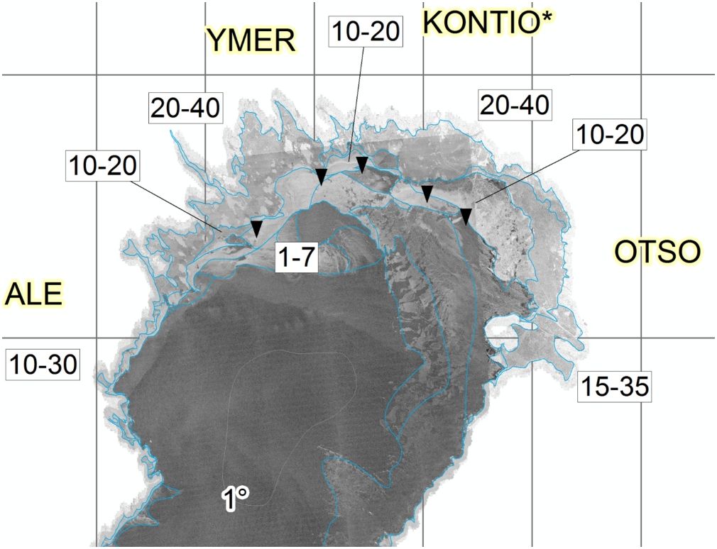
Figure 6. A Sentinel-1 SAR satellite image over the Northern Bay of Bothnia as viewed in the ice charting tool Vanadis, with the ice analyst’s division of the sea ice into polygons.

3.2.2 Optical and Infrared sensors

When a satellite orbit passes over the Baltic Sea, a medium resolution (250 to 1000 m) spectrometer imagery usually cover the whole Baltic Sea. Unfortunately, the use of optical and thermal infrared imagery is heavily restricted by cloud cover, and optical imagery also by the short days during the early and mid-winter. The benefit of using optical imagery increases from March with more daylight and clearer skies. In cases when satellites operated in the optical bands offer a clear view of the ice situation, it often makes distinction between ice and open water remarkably easier than can be done from SAR imagery. This benefit is further accentuated during the melt period, since wet snow on ice or wet ice surface attenuate the SAR backscattering from sea ice, resulting to reduced contrast in the SAR imagery (Howell et al., 2018; Mahmud et al., 2020).

3.2.3 Satellite data transmission and preprocessing

The satellite data are ordered in advance by the FMI ice analysts using a dedicated online ordering system. The satellite data are received at the Sodankylä ground station located in northern Finland. ESA Sentinel data are available in near-real-time (NRT) though the Copernicus data hubs with their user interface and also through ftp. The data from the other satellites are available from ftp sites provided by the satellite operators or ESA. The data are transmitted to ftp by frequently polling the ftp sites and retrieving the new data as soon it is detected by the polling script. After data transmission, the data are georectified to Mercator projection with a center latitude of 61 2/3 degrees. This projection is similar to the one used in the Baltic Sea nautical charts. After the georectified SAR images are calibrated, an incidence angle correction is applied to them and also thermal noise reduction is performed. Finally, a land mask is applied to remove the unnecessary land areas, thus enabling reduction of data size. The images are then provided in GeoTIFF format for the ice services and for the automated algorithms applied in CMS. The data are also stored for further use in research.

4 Products and services

4.1 Ice chart

The primary product of the sea-ice monitoring is the ice chart. The daily ice charting is done by one sea ice analyst. The analysis is finished slightly after noon, by when most satellite images from that same morning can be utilized. As the whole charted area rarely is fully covered by imagery every morning, images can be ordered to cover the operationally most important areas almost daily (where the navigation in ice is the most intense). Occasionally, the ice analysis is also based on evening passes from the day before. The aim is that the date of the chart ultimately corresponds to imagery from the same morning. Used imagery are mainly dusk-pass SAR but also optical imagery from before noon (MODIS, VIIRS, Sentinel-2). Additionally, satellite image information, which always represents a specific time in the past, can be altered with observations from icebreakers, coastal radars and drift buoys. The final ice analysis thus depends on all the used data, on the prevailing weather and the interpretation of the ice analyst.

The ice chart is compiled in vector form, consisting of polygons to which the ice analyst applies one parameter value to represent the general ice features of the defined area as accurately and consistently as possible. The polygon division is chosen to collect the same type of ice as comprehensively as possible. Thus, the ice charts cannot indicate exact values for every location, but the used ground truth is rather echoed as a general representation and distribution for the defined polygons. This does create some uncertainty when estimating specific local conditions and this feature needs to be taken into account by the user. The discretized nature of the ice chart is visually easy to interpret, but when used for, say, satellite image or sea-ice model validation, the characteristics of the data needs to be understood.

The manually analysed ice chart is based on the following information sources:

1. Satellite images.

2. Icebreaker observations.

3. Manual observations from coastal stations.

4. Ice drifters.

5. Numerical prediction models.

6. Coastal radars.

As almost all source data used in the ice charting include higher degrees of detail than can be expressed in the ice chart analysis, certain aspects need to be considered by the users. First of all, the representation of the ice situation is relative to the scale of the entire Baltic Sea, fitted to one A3 page. Secondly, focus is given to areas where vessel traffic is hampered by ice and where icebreaker assistance is needed. The main purpose of the ice chart, namely, to give the shipping sector and ice navigation a general view of the ice resistance in each zone. The high resolution of satellite image bitmaps is difficult to match with the highly discrete form of the ice chart, in which we may choose to include vast areas in one polygon based on some chosen feature. This could be high concentration combined with a fairly similar level-ice thickness, thus possibly neglecting a high variation in ice deformation, even if it can be identified in SAR texture. In the PDF ice chart, deformed ice therefore is indicated by symbols for ridged ice, rafted ice and brash ice barriers.

4.2 Ice chart parameters

4.2.1 Ice type

The ice type definitions used in the ice charts have slightly evolved over the course of time. There have been variations in the way ice type and the concentration have been defined. The harmonized standard of today is the WMO Sea-Ice Nomenclature (WMO, 2014a) and the ice types used in the Finnish-Swedish Baltic Sea ice chart are shown in Figure 7.

Figure 7

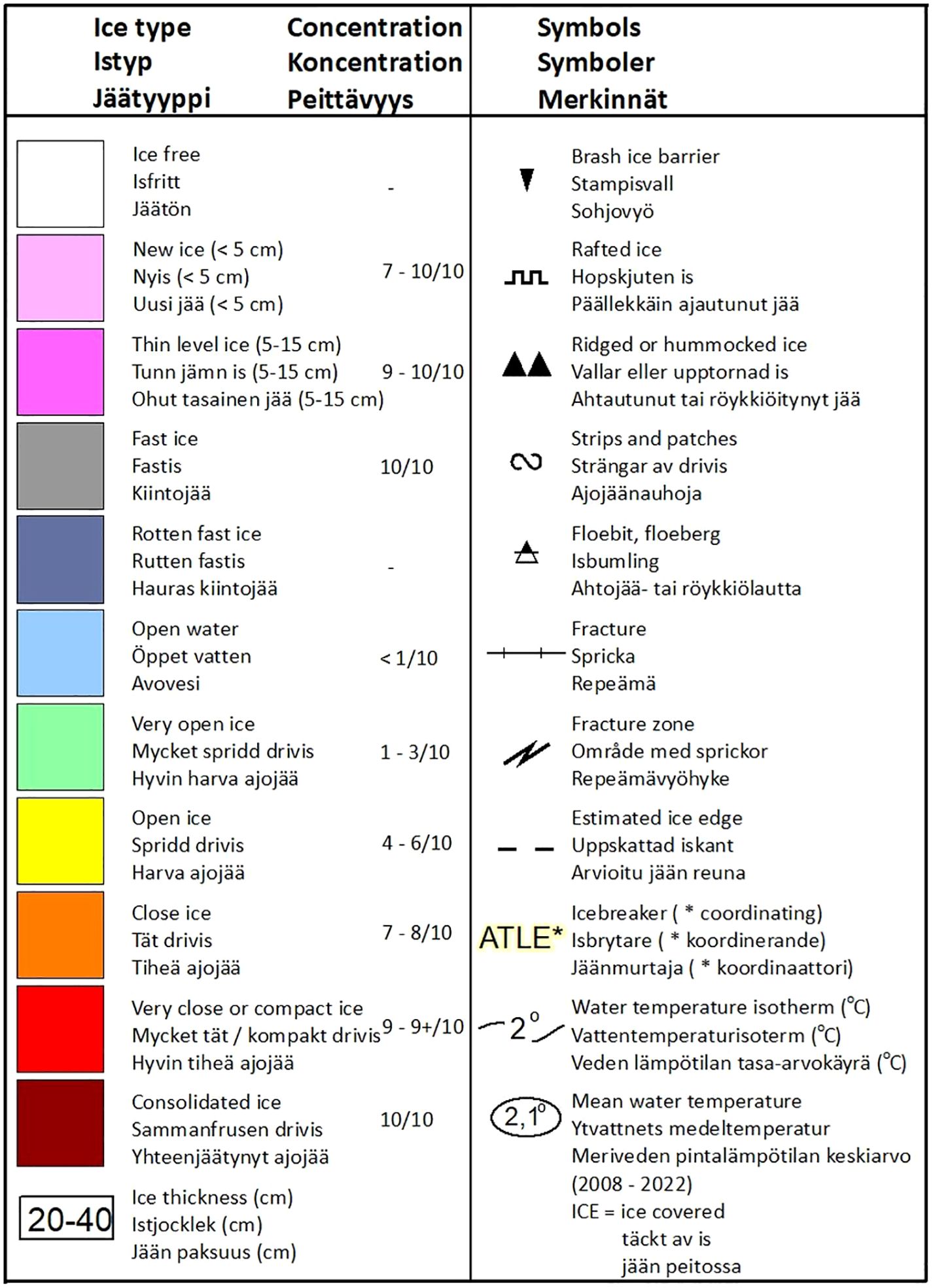
Figure 7. Legend of the ice chart explaining the meaning of colours, symbols, annotations and text used.

4.2.2 Concentration

The concentration indicates the fraction of the sea surface in tenths, where 0/10 means ice-free and 10/10 full ice coverage. The ice type and concentration are partly linked to each other, as most of them include a concentration value or interval.

4.2.3 Ice thickness

The given ice thickness describes the thickness of level ice, meaning that all forms of deformed ice are excluded from the thickness values. This also means that the thickness reading, at least in principle, should correspond to the thickness of thermally grown ice. This has been the leading principle throughout the history of ice charting. In the ice charting tool, ice thickness has three input categories: minimum, mean and maximum ice thickness. These make it possible to indicate what stages of development are included within the area and thus define a rough thickness distribution for the given polygon. In the PDF chart’s ice thickness annotations, however, only the minimum and maximum are indicated as a total interval.

- The minimum thickness indicates the youngest form of ice.

- The mean thickness is intended to describe the typical, or most common, occurring ice thickness. This value would therefore rather indicate the mode in a thickness distribution.

- The maximum thickness indicates the highest stage of development.

The thickness readings have occasionally been compared to electromagnetic (EM) ice thickness measurements performed and the mode of the observed thickness histograms have matched fairly well with the ice chart readings.

Observations of drift ice are almost entirely based on icebreaker observations, and the icebreaker crews have the best experience for assessing the different features of the ice, like how to determine ice thickness and concentration. The ice analyst on duty nevertheless performs a quality check on the incoming icebreaker observations.

Maps digitised from archived old paper ice charts no longer contain original observations, so the average thickness has been set to the average of the minimum and maximum, but rounded to an accuracy of 5 cm, and up rather than down.

4.2.4 Ice deformation

The forms of deformed ice indicated in the ice charts are ridged ice (Figure 8), rafted ice and brash ice. One polygon parameter used in the Finnish-Swedish ice chart is the Degree of Deformation (DoD). It’s a numeral on a six-digit scale (0: undeformed, 1: rafted ice, 2: slightly ridged ice, 3: moderately ridged ice, 4: heavily ridged ice, 5: brash (typically indicating a compacted ice edge zone of brash ice, connected to the brash ice barrier symbol).

Figure 8

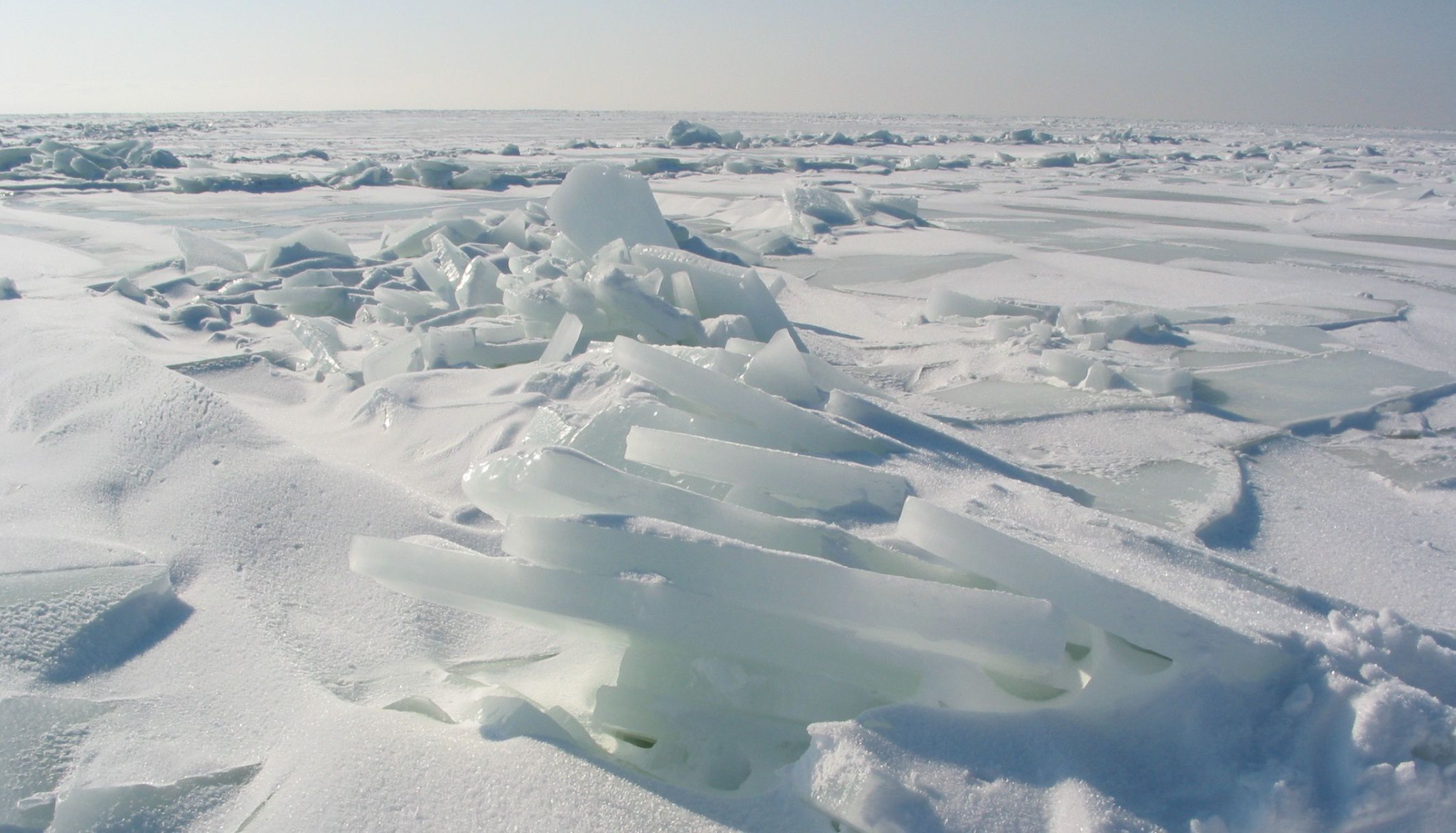
Figure 8. Ridged drift ice field in the northern Bay of Bothnia (photo: Patrick Eriksson).

The ice analyst determines the degree of deformation (DoD) both from satellite imagery and based on observation reports from the icebreaker fleet. The icebreaker observations are considered as more reliable ground truth and are therefore the primarily reference when setting the DoD value. The satellite imagery, on the other hand, indicates the aerial distribution of the deformation zones.

As all parameters applied to one polygon, the DoD gives only one numeral for the whole polygon area. Consequently, it is a poor indicator of ice ridge distribution and can only give a flattened average of the deformation rate in the specific polygon.

Also, the scale of DoD is highly practical and simplified, based on how the deformed ice affects icebreaking operations and navigation in ice. Therefore, the categories are non-physical, applied by empirical judgment as reported by icebreaker bridge officers and the ice analyst, and have to be treated accordingly.

4.2.5 Sea surface temperature

The Sea Surface Temperature (SST) is drawn in the ice-free regions of the ice chart. Isoterms with one-degree intervals are drawn based on in-situ observations from buoys, coastal stations and vessels. Also, satellite-based analysis products and numerical oceanographic models are used.

The SST as part of the operational ice chart is an important parameter for the users as it indicates the cooling of the surface water, and that way anticipates the onset of freezing. In the ice chart, also statistical means of the SST are shown for selected locations, which tells how the season is progressing in a climatological reference.

4.3 Output and distribution

The main issuing format is the visual chart, published on the FMI website and distributed by e-mail and other web applications (Figure 9). All the coding of the chart follows the guidelines of the WMO sea ice nomenclature, and specifically the one assigned to Baltic Sea conditions (WMO, 2014b). The ice information is depicted by the parameters and symbols presented below.

Figure 9

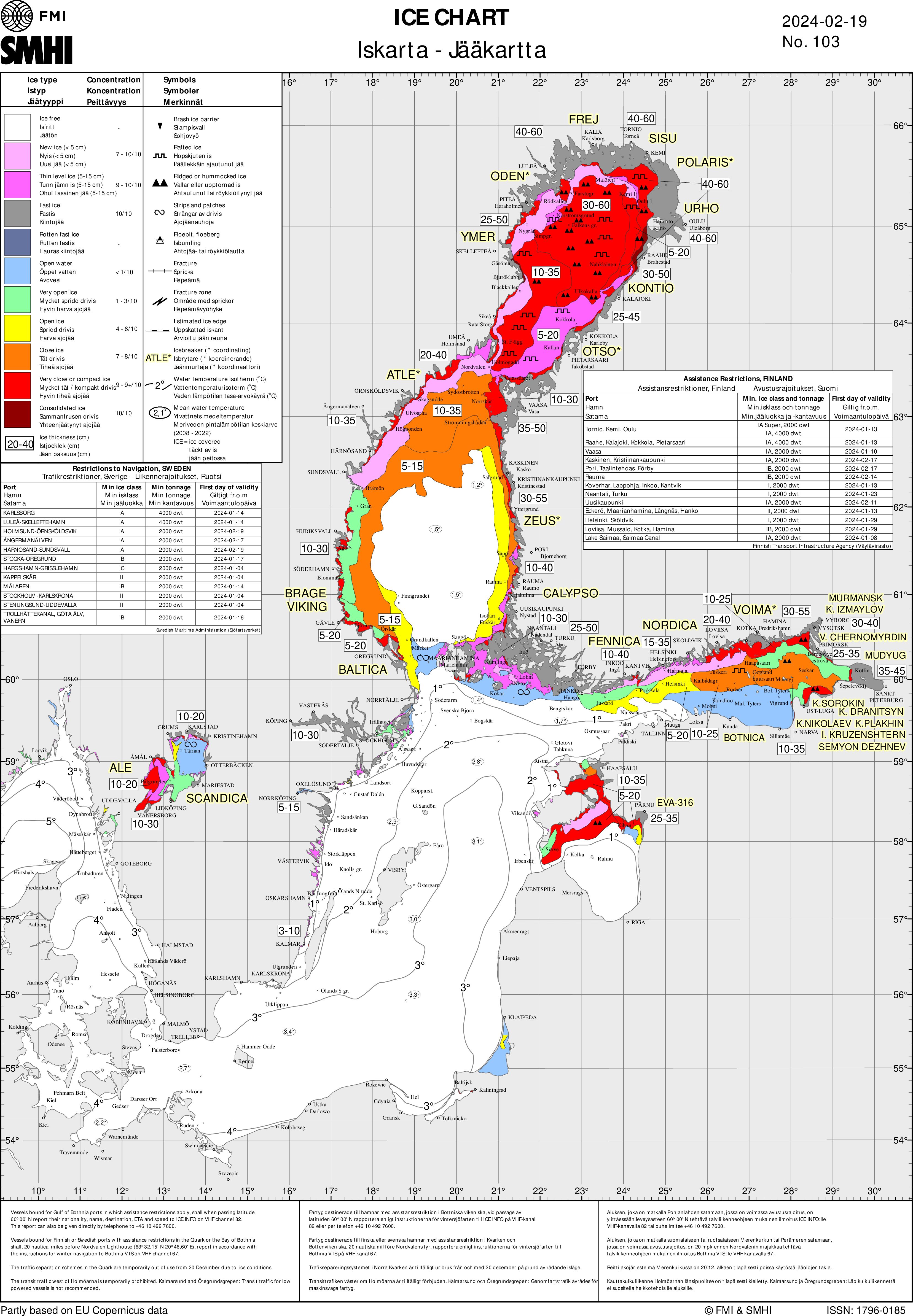
Figure 9. The Finnish-Swedish ice chart of 19th February 2024. On the back page there is more traffic information for navigation.

The output formats of the ice chart are printable charts, NetCDF grids and the Shape-like SIGRID-3 format (although currently still in Beta phase). Today the printable chart is in PDF format as colour and black-and-white versions.

As the ice charting tool makes it possible to store more parameters to the polygons than are shown in the PDF chart, these parameters can be included in numerical output formats like grid files or digital vector formats. Possible parameters in the numerical outputs are:

● Ice type.

● Ice concentration.

● Level ice thickness (minimum, mean, maximum).

● Degree of deformation.

● Sea surface temperature.

4.4 Ice codes

Publishing of the ice codes in Finland began in 1921. The ice codes contain information of the sea ice conditions along the Finnish fairways and adjacent sea areas in a very condensed form. Initially each individual code consisted of only two digits describing the ice conditions, but over the years they have gone through a few steps of changes before the Baltic Sea ice code, currently in use, was adapted in 1981 (SMHI, 1981).

The ice codes are series of character strings containing an area definition, followed by four digits describing the ice conditions. The first of these four digits describes the amount and arrangement of ice, the second digit the stage of development, the third digit the topography or form of ice, and the last digit the navigation conditions in ice.

For example, the code BB1–8376 means that on the fairway from Oulu harbours to Kattilankalla (BB1) there is fast ice (8) of 15–30 cm thickness (3) with hummocks or ridges (7) and a specific ice class and size is required of a vessel to be allowed icebreaker assistance (6).

Ice code production for the winter starts with the setting of first assistance restrictions to Finnish ports by the winter navigation authorities, coinciding with the start of daily ice charting and the start of ice reports. They are distributed using the GTS network (Global Telecommunication System) as NAVTEX messages and shared with all the other ice services around the Baltic Sea, as agreed by the Baltic Sea Ice Meeting. As the ice code format is uniform within the Baltic Sea ice service community, its compressed and easily interpreted nature has been used as a practical source of information, giving a comprehensive picture of the whole sea area in daily time steps. Based on this, the ice codes are used for statistical analyses, like the ones compiled on the Baltic Sea Ice Services’ web page (BSIS, 2025).

4.5 Ice report

Finnish ice reports have been read on the radio since the 7th of January 1927. Today, the ice report is a literal description of the ice conditions relevant for the traffic to the Finnish ports, followed by information from the winter navigation authorities. It is published daily during the winter navigation season. The first reports are issued when the winter navigation authorities set the first assistance restrictions for the season and the last when the last ice chart is published.

The ice report consists of two parts. The first part describes the ice situation in the whole Baltic Sea, with an emphasis on the Finnish sea areas and the Lake Saimaa and Saimaa Canal route during its winter navigation season. The ice report focuses on the ice conditions along fairway areas, describing the type of ice, its thickness and deformation stage. Features with importance to navigation, such as brash ice barriers, ice pressure areas, cracks and leads, are also described. There is an endeavour to keep the ice report relatively short, but at the same time it must contain all the required and critical information.

The data sources for the ice report are the same as for the ice chart, but the report is published earlier than the chart, around noon.

The second part of the ice report contains information from the winter navigation authorities. The operating icebreakers are listed along with their operation locations. The current assistance restrictions to Finnish ports are given, as well as coming changes to these. Other announcements from the winter navigation authorities concerning winter navigation are also mentioned, like reporting rules and possible exceptions to navigation directives caused by the ice conditions.

The ice report is written in Finnish, Swedish and English. The text is published on the FMI website and distributed via e-mail. The Finnish Broadcasting Company (YLE) reads the report in Finnish and Swedish on its radio channels and the Maritime safety radio, Turku Radio, reads it in English.

4.6 Ice forecasts

The Ice Service produces a 10-day ice condition development forecast for the Finnish Transport Infrastructure Agency once a week. The forecast describes the daily development of ice conditions in Finnish sea areas, including ice movement, thickness growth, and deformation. Also zones of anticipated ice pressure are mentioned, to the extent it can be evaluated based on both icebreaker observations and sea-ice models. The forecast is based on the initial conditions and the wind and temperature forecasts for the coming days. A numerical sea-ice forecast model is utilized for the first few days. The ice model used is the NEMO-SI3. Icebreaking operations use the forecast for planning winter navigation and the vessel assistance activity. Additionally, a weekly ice thickness forecast for Finnish ports is made for the Finnish Transport Infrastructure Agency. Ice thickness growth is predicted using the formula defined by HELCOM (HELCOM, 2004) and is based on the cumulative freezing degree days. The initial ice thickness in the forecast is obtained from ice observations. If no ice observation is available, a calculated value is used as the initial ice thickness. The nearest weather observation station and temperature forecast are used for calculating the freezing degree days.

In the monthly seasonal forecast SEASON (Seasonal Forecast), the extent and thickness of ice in the Baltic Sea, as well as the number of icebreakers required, are predicted on a monthly basis. The forecast utilizes the prevailing ice conditions and sea temperature at the initial situation, comparing them to similar situations in previous winters. Based on data from past winters, it is possible to estimate how the ice conditions will develop if the weather is predicted to follow the observed weather of those winters. The weather forecast primarily uses long-term forecasts from ECMWF. Due to uncertainties in the weather forecasts, the seasonal ice forecast relies heavily on the professional experience of ice experts.

4.7 Ice season descriptions and maximum ice chart

Each year, after the season ends, the Ice Service writes a description of the past ice season. These descriptions have been made since season 1913/1914 (Granqvist, 1921), and since the season of 1995/1996, the reports have been published on the institute’s website in Finnish, Swedish, and English. Currently, the description is a verbal summary of the evolution of ice conditions during the winter, and it includes information on ice thickness and a climatic comparison of the length of the ice season. The description also includes the maximum ice extent in the Baltic Sea and the date of this maximum. In the calculation, areas with at least 1/10 ice coverage are considered ice-covered.

Along with the ice season description, a chart of the maximum ice extent is also published on the website, see example in Figure 10. Compared to the regular ice chart, this chart includes additional information on icebreaking activities and assistance restrictions in Finland and Sweden. Nowadays, ice areas in the maximum ice chart are not drawn separately afterward; instead, the operational ice chart published on that day is used.

Figure 10

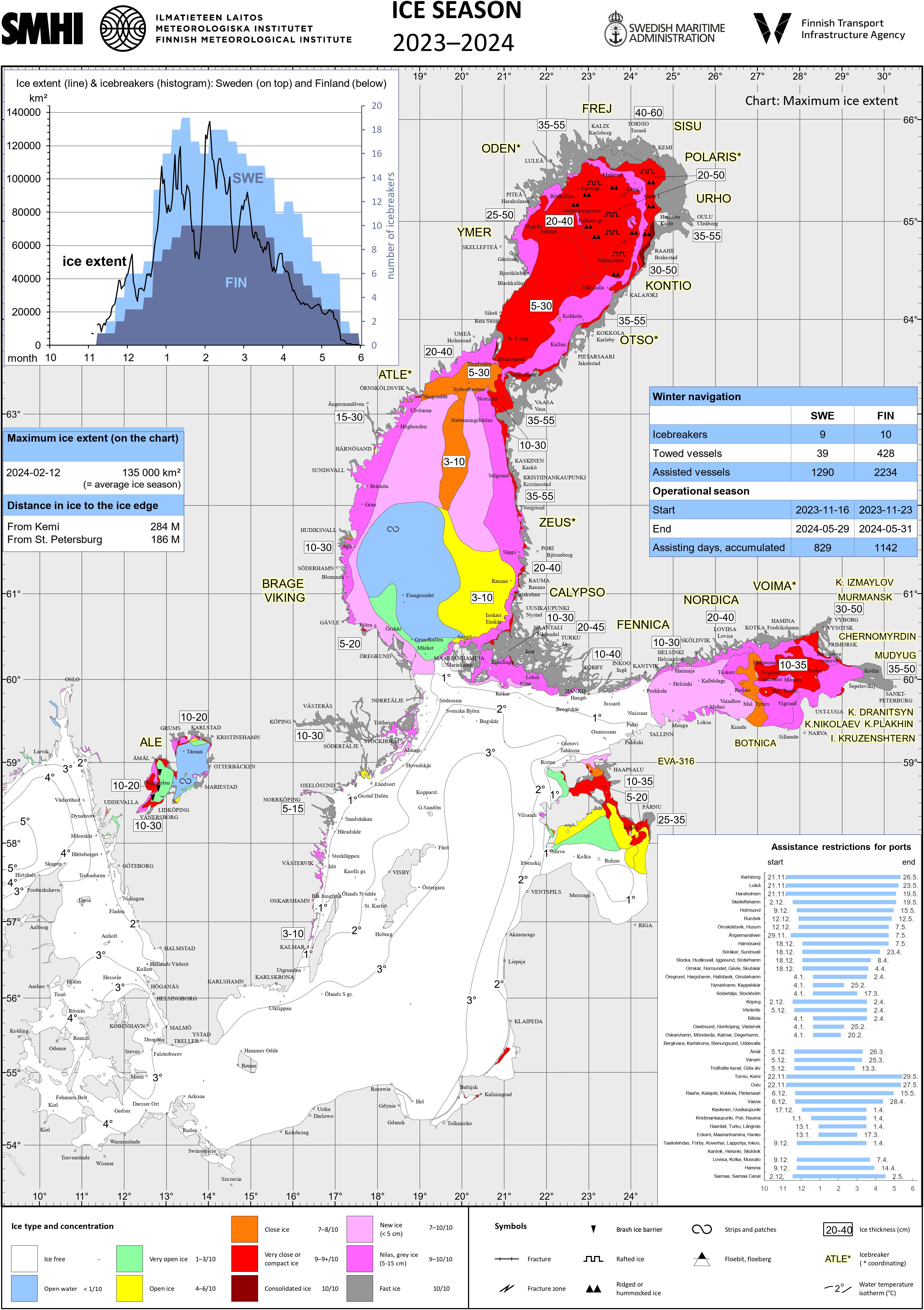
Figure 10. The maximum ice chart of season 2023/2024. Since 2018 the product has also included data of the winter navigation of the season, like how much assistance was done.

4.8 Data and product storages and archives

The ice service archives its operational products and part of the data used in their production. The latest ice chart is available in PDF format at FMI web pages and archived ice charts can be delivered at request. Ice charts in PDF format are available from ice season 2001. The ice analysis resulting in the printable ice chart is stored in PostGIS databases and used in production of gridded and vector format datasets. Digitized ice chart data is available weekly from 1980.

The gridded ice chart data is produced in NetCDF format in ¼ nautical mile nominal resolution. It contains eight parameters: land-sea mask, ice type, total ice concentration, minimum ice thickness, average ice thickness, maximum ice thickness, sea ice degree of deformation and sea surface temperature. The data is compatible with JCOMM Electronic Chart Systems Ice Objects Catalogue (JCOMM. Joint Technical Commission for Oceanography and Marine Meteorology (JCOMM) and Expert Team on Sea Ice, 2014). Currently ice chart data in NetCDF format is available daily from 2007 and weekly from 1980. Occasionally, there are short gaps in the NetCDF data series, since on some dates the ice chart hasn’t been produced due to national public holidays and weekends near the very end of the season. Additionally, there is a gridded CMS product (004) with ice concentration and average ice thickness data in 1 km nominal resolution.

The vector ice chart data is produced in a shapefile format called SIGRID-3 (WMO, 2010). The SIGRID-3 files contain most of the data included in the ice analysis, except for the ice type, which is not recognized by the SIGRID-3 standard. Daily production of SIGRID-3 began at the start of ice season 2019.

Published ice reports and ice codes are archived by the ice service. In digital format they’re available from ice season 2011 and can be delivered at request.

The coastal ice thickness observations submitted via electronic form are available through FMI open data from 2016. The measurements from ice season 1991 onwards are stored in digital format, while older coastal ice observations are currently archived in original measurement forms on paper and available in ice season publications by the Finnish Institute of Marine Research.

Satellite images used in the ice analysis and sea ice forecasts produced for the winter navigation authorities are archived, but not available to the public. When there are multiple satellite images available for the same sea area during the analysis, only the most suitable image is archived. Images not containing any ice are not archived, even when used in the analysis to see if there is any ice in the area.

4.9 Copernicus marine service and its relation to the ice service

The Copernicus Marine Service (CMS, https://marine.copernicus.eu) is the marine component of the EC Copernicus programme, and forms one of the six key thematic components of Copernicus. Copernicus Marine is devoted to the monitoring of the ocean worldwide, with a focus on satellite-derived data but also with in situ (measurements made on site) thematic assembly centres (TAC’s) along with model-based products, and offers free access to a catalogue of about 200 standardized and quality-controlled products describing the physical, sea ice and biogeochemical features of European seas and the Global Ocean.

The CMS sea ice TAC (SITAC) is coordinated by Met Norway and the SITAC Baltic Sea production unit is at FMI. CMS provides NRT satellite imagery from ESA’s Sentinels and also so-called Copernicus Contributing Missions (CCM) data for use in ice charting and automated sea ice products. FMI receives CCM data from RADARSAT-2, Radarsat Constellation Mission (RCM), TerraSAR-X, COSMO-SkyMed and PAZ. Also some other SAR instruments, such as ICEYE have been in operational test use.

The CMS is in close connection with the FMI Ice Service. The SAR data for the ice charting is received in near-real-time (NRT) through CMS and data derived from the FMI ice charts are provided to CMS SITAC. CMS enables that the data from the ESA Sentinels are available with minimal time gap from the data acquisition and also the coordinated availability of CCM data. Further, the access to CCM data makes it possible to fill acquisition gaps caused by the fixed predefined data acquisition plans of Sentinel-1 and RADARSAT-2.

The CMS SITAC Baltic Sea production unit at FMI has two major product groups: SEAICE_BAL_SEAICE_L4_NRT_OBSERVATIONS_011_004 (in the following shortly 004) and SEAICE_BAL_SEAICE_L4_NRT_OBSERVATIONS_011_011 (011). The 004 data sets are directly based on digitized FMI ice charts and 011 data sets are automated products based on the EO data. The area covered by the SITAC products is the whole Baltic Sea.

The gridded CMS ice analysis (004) products in CMS are sea ice concentration (SIC) and average sea ice thickness (SIT). These products are both given in a 1 km nominal resolution corresponding to that of the FMI ice chart. These CMS products are provided daily after completion of the daily ice chart.

The 011 products are mainly based on C-band SAR imagery from Sentinel-1, RADARSAT-2 and RCM. X-band SAR data from TSX, CSK and PAZ are used for SIT products only. The CMS 011 datasets currently include SIT., SIC and sea ice drift (SID), as well as sea ice extent (SIE) derived directly from SIC. The products are produced after reception of a SAR image and a SIT mosaic product is updated twice daily if new SAR data are available. The SID dataset is updated each time when overlapping SAR data with a time difference less than three days are available.

The CMS SITAC algorithms for the SIT estimation are described in more detail in (Karvonen et al., 2003, 2008; Karvonen and Cheng, 2024), the ice drift estimation method in (Karvonen, 2012b) and the SIC estimation algorithm in (Karvonen, 2017).

Starting from the beginning of the Baltic ice season 2020–2021 also another 011 dataset of SIT is provided as part of CMS. These data are similar to the abovementioned 011 SIT, except that they are computed from the Sentinel-1 IW mode (VV/VH) data.

The CMS products are evaluated after each season w.r.t. reference data sets. These data sets include SIT observations from Finnish and Swedish icebreakers, coastal SIT measurements, SIC based on microwave radiometer data from Universities of Hamburg and Bremen, and buoy measurements of the ice drift. The evaluation results are published in the annual CMS data quality reports, issued after each Baltic Sea winter season.

5 Sea ice research

Studies related to the Baltic Sea ice have been conducted over 100 years, first motivated by the development of winter navigation and later including geophysical studies on the Baltic Sea ice properties and climatology. Since the 1950’s, studies have focused on large scale problems, such as sea ice climatology and dynamics, sea ice thermodynamics, sea ice ecology, thickness distributions of level ice and deformed ice, ice ridge statistics (e.g. ridge density), mechanical properties of sea ice (e.g. shear strength of ridges), and on sea ice properties particularly relevant for microwave remote sensing (e.g. surface roughness). Sea ice remote sensing studies started in mid 1970s and intensified in late 1980s and 1990s for the usage of SAR imagery in operational sea ice monitoring.

Theoretical geophysical modelling of sea ice has included the following topics: 1) Seasonal sea ice climate, e.g (Haapala, 2000), 2) Sea ice dynamics, e.g (Zhang, 2000), and 3) Sea ice thermodynamics and air-ice interaction, e.g (Cheng, 2002). These studies are mainly focused on the numerical model constructions, validations, and to better reproduce sea ice physics with numerical modelling on the basis of seasonal and synoptic time scales. In general, the large-scale ice conditions, like ice extent, in the Baltic Sea are well known, but little is still known about the small-scale properties of the ice, the processes during initial ice formation, and the temporal development of the ice properties (Granskog, 2004). The main reason for this is the need of time consuming and expensive logistical efforts for studying sea ice processes in harsh field conditions.

5.1 Remote sensing of the Baltic Sea ice

There is a long history of Baltic Sea ice remote sensing and geophysics research conducted at FIMR and later at FMI for development of operational FIS services and products. Remote sensing research since late 1980’s has been heavily focused on the usage of the SAR imagery for automatic retrieval of various sea ice parameters, like ice types, degree of deformation, and sea ice concentration. FIS has used SAR imagery since 1992 with the availability of ERS-1 SAR.

Investigations on the feasibility of microwave remote sensing for the Baltic Sea ice monitoring started in 1975 (Hallikainen, 1992). The first research campaign was Sea Ice-75 organized jointly by Finland and Sweden. In this campaign first airborne radar (10 GHz side-looking airborne radar (SLAR)) and radiometer (0.6 and 5 GHz) measurements were conducted. It was followed in 1987 by the Bothnian Experiment in Preparation of ERS-1 (BEPERS-87) pilot study (Leppäranta and Hakala, 1992). This study included the first airborne SAR measurements over the Baltic Sea ice with a French X-band SAR. BEPERS-88 study included first airborne C-band SAR measurements conducted by Canada Centre for Remote Sensing (CCRS), and first C- and X-band helicopter-borne scatterometer measurements conducted by Laboratory of Space Technology of Helsinki University of Technology (Leppäranta and Thompson, 1989). In the late 1980’s the research work intensified for studying the use of the ERS-1 SAR images for the Baltic Sea ice monitoring. First ERS-1 images, and also, the first spaceborne SAR images over the Baltic Sea ice, were acquired in the winter 1992. In general, remote sensing research has been heavily focused on the usage of the SAR imagery for automatic retrieval of various sea ice parameters, like degree of deformation, Optical and TIR imagery has been used only for development and validation of SAR based sea ice products.

Utilization of spaceborne microwave radiometer data for the Baltic Sea ice monitoring has not been studied much. The main reason for this is the coarse resolution of the radiometer data, e.g. in the current AMSR2 radiometer data the resolution is from 35 by 62 km (6.9 GHz channel) to 3 by 5 km (89 GHz channel) (Maeda et al., 2016), compared to area of the Baltic Sea and its typically rugged coastline with many islands (land contamination of measured ocean/sea ice brightness temperatures). Few studies have been conducted for the sea ice concentration estimation (Hallikainen and Mikkonen, 1986; Grandell et al., 1996).

Research work on the usage of laser and radar altimeters for retrieving Baltic Sea ice properties has also been limited as they have little usage in the operational monitoring due to spatial and temporal sparseness of the altimeter ground tracks. Estimation of degree of ice ridging has been demonstrated (Fredensborg Hansen et al., 2021). Uncertainties in sea ice thickness estimation with Cryosat-2 radar altimeter rise asymptotically towards thinner ice less than 1 m thick (Ricker et al., 2017). As level sea ice in the Baltic Sea is generally less than 1 m thick, the radar altimeter based ice thickness estimation can be considered mostly useless in the Baltic Sea. In the Arctic, the Cryosat-2 observations have been successfully merged with SMOS microwave radiometer observations, but in the Baltic SMOS observations are likely to suffer from land contamination (Li et al. 2017; Maaß et al., 2015).

In the following is a list of the Baltic Sea ice properties which can be estimated using SAR data alone or together with other data. Methods for the sea ice property estimations are also shortly described. This list is mainly based on studies with the C-band dual-polarized SAR data which is the main operational satellite data used by the Finnish Ice Service. Only some of the methods are used for operational sea ice products.

● Sea ice extent and concentration: with SAR data only (Karvonen et al., 2005; Karvonen, 2012a; Karvonen, 2014), and combination of SAR and microwave radiometer data.

● Sea ice thickness based on combination of ice chart SIT data and SAR image statistical analysis (Karvonen et al., 2003, 2004; Similä et al., 2005), or empirical relationship between ice freeboard derived from airborne laser altimeter data and SAR backscatter (Similä et al., 2010).

● Sea ice types (Karvonen, 2004) based on statistical SAR image segmentation and texture feature classification.

● Sea ice drift/dynamics based on time series of SAR images (Karvonen, 2012).

● Land fast ice extent based on time series of SAR images (Karvonen, 2018).

● Degree of deformation (Gegiuc et al., 2018) based on statistical SAR image segmentation and texture feature classification.

● Estimation of ice-going ship speed by Random forest regression between local statistical SAR features and AIS data (Similä and Lensu, 2018).

Few case studies have utilized SAR interferometry for estimation of small horizontal deformations in level ice or displacements of level ice, e.g (Dammert et al., 1998,; Marbouti et al., 2017). As Sentinel-1 has long temporal baseline SAR interferometry, it only can be applied over fast ice, and snow and sea ice conditions should not change much between acquisitions in order to have high coherence. Polarimetric SAR remote sensing of the Baltic Sea ice is still in infancy, mainly due to the very limited amount of data available so far. Likewise, multifrequency SAR approaches have not been used much due to limited availability of co-incident SAR data.

In many SAR algorithms for retrieval of sea ice properties, FMI ice charts and their concentration and degree of ice ridging fields, have been used as training data.

Machine-learning methods and neural networks have traditionally played a major role in the sea ice analysis algorithms that are based on EO data, and the development in this sector has proven to be ongoing. For instance, models for sea ice concentration estimation and degree of deformation using a modified U-net (Ronneberger et al., 2015) neural network with hyper-parameter optimization are under development and currently in test phase at FMI. These methods will be applied in the operational Copernicus Marine Service sea ice products in the near future. According to the preliminary tests, these new methods will improve the estimation and classification accuracy by a few percentage points.

The above-mentioned sea ice research activities at FMI, and formerly at FIMR, emphasize the fact that the research part is an integral part of the operational Ice Service and its capabilities.

The research projects in Finland on the development of operational sea ice classification algorithms for spaceborne SAR data have also included following tasks: (1) basic research in backscatter signatures of sea ice, e.g. statistics for various ice types and effect of snow wetness in the statistics, e.g (Mäkynen and Hallikainen, 2004: Mäkynen, 2007), (2) theoretical modelling of backscatter signatures, e.g (Manninen, 1992; 1996a; 1996b), (3) field campaigns to gather ground truth data and radar data with airborne, coastal and shipborne radars, (4) development of end-user software for interpretation and use of the sea ice products, and (5) various issues of data delivery to end-users at ships, e.g (Karvonen and Simila, 2002). Tasks (1)-(3) support the development and validation of the SAR classification algorithms.

6 Future outlook

In this paper, the concept of ice monitoring at the Finnish Ice Service, and its focus on the winter navigation needs, has been presented. The over 100 years of ice monitoring and ice charting has always responded to the specific evolution in shipping in ice and to the technological advances in all related fields. The future evolvement is not that easy to foresee, but the sea ice services will nevertheless continue to adapt to the circumstances ahead.

Climate change has for some time already appeared as one constraint to the development of the ice service. But even if the average winters aren’t as long as they used to be, harsh winters are still to occur and difficult navigational conditions still will cause trouble, especially in the northernmost basins of the Baltic Sea. Milder winters result in more mobile ice, which even causes new obstacles at sea. Formation of difficult brash ice zones seems to have increased. Phenomena like these may demand new ways of describing the ice conditions and the forecasting and information flow needs to be able to respond to the ever-tighter requirements.

As the amount of available satellite imagery is increasing and, simultaneously, the demand for higher levels of detail in the service products, the manual analysis process used during the past few decades is facing new challenges. In the near future, new automated or semi-automated methods have to be developed in order to handle the growing amounts of data.

One thing is still clear, however. The need for safe and efficient ice navigation will not disappear any time soon, and ice services will still be needed, in one form or another.

Author contributions

PE: Conceptualization, Investigation, Project administration, Supervision, Writing – original draft, Writing – review & editing. JV: Writing – original draft, Writing – review & editing. NT: Writing – original draft, Writing – review & editing. AJ: Writing – original draft, Writing – review & editing. AA: Writing – original draft, Writing – review & editing. MM: Writing – original draft, Writing – review & editing. JK: Writing – original draft, Writing – review & editing. AK: Conceptualization, Project administration, Writing – original draft, Writing – review & editing.

Funding

The author(s) declare that no financial support was received for the research and/or publication of this article.

Conflict of interest

The authors declare that the research was conducted in the absence of any commercial or financial relationships that could be construed as a potential conflict of interest.

Generative AI statement

The author(s) declare that no Generative AI was used in the creation of this manuscript.

Any alternative text (alt text) provided alongside figures in this article has been generated by Frontiers with the support of artificial intelligence and reasonable efforts have been made to ensure accuracy, including review by the authors wherever possible. If you identify any issues, please contact us.

Publisher’s note

All claims expressed in this article are solely those of the authors and do not necessarily represent those of their affiliated organizations, or those of the publisher, the editors and the reviewers. Any product that may be evaluated in this article, or claim that may be made by its manufacturer, is not guaranteed or endorsed by the publisher.

References

Berglund R. and Eriksson P. B. (2015). “National ice service operations and products around the world,” in Shen H. (Ed.), Cold Regions Science and Marine Technology, vol. 2, pp. 1–20. EOLSS Publishers. Available online at: https://www.eolss.net/ebooklib/bookinfo/cold-regions-science-marine-technology.aspx (Accessed September 23, 2025)

Google Scholar

BIM (2020). Baltic Sea Icebreaking Report 2019-2020. Baltic Icebreaking Management. Available online at: https://www.baltice.org/api/media/get?folder=icebreaking_reports&file=BIM%20Report%202019-2020.pdf (Accessed August 14, 2025).

Google Scholar

BSIS (2025). Sea ice statistics Baltic. Available online at: https://www.bsis-ice.de/statistik/Stationindex.html (Accessed August 14, 2025).

Google Scholar

Cheng B. (2002). On the modelling of sea ice thermodynamics and air-ice coupling in the Bohai Sea and the Baltic Sea (Finland: Finnish Institute of Marine Research – Contributions).

Google Scholar

Dammert P. B. G., Leppäranta M., and Askne J. (1998). SAR interferometry over Baltic Sea ice. Int. J. Remote Sens. 19, 3019–3037. doi: 10.1080/014311698214163

Crossref Full Text | Google Scholar

FMI (2025). Sea Ice statistics. Available online at: https://en.ilmatieteenlaitos.fi/icestatistics (Accessed January 7, 2025).

Google Scholar

Fredensborg Hansen R. M., Rinne E., Farrell S. L., and Skourup H. (2021). Estimation of degree of sea ice ridging in the Bay of Bothnia based on geolocated photon heights from ICESat-2. Cryosphere 15, 2511–2529. doi: 10.5194/tc-15-2511-2021

Crossref Full Text | Google Scholar

Gegiuc A., Simila M., Karvonen J., Lensu M., Mäkynen M., and Vainio J. (2018). Estimation of degree of sea ice ridging based on dual-polarized C-band SAR data. Cryosphere 12, 343–364. doi: 10.5194/tc-12-343-2018

Crossref Full Text | Google Scholar

Grandell J., Johannessen J. A., and Hallikainen M. (1996). Comparison of ERS-1 AMI wind scatterometer and SSM/I sea ice detection in the Baltic Sea. Photogrammetric J. Finland 15, 6–23. Available at: https://hdl.handle.net/10013/epic.21482 (Accessed September 23, 2025).

Google Scholar

Granqvist G. (1921). Jäät vuonna 1913–14 Suomen rannikolla. Merentutkimuslaitoksen julkaisu N:o 3 Helsinki: Valtioneuvoston kirjapaino. Available at: http://hdl.handle.net/10138/158441 (Accessed September 23, 2025).

Google Scholar

Granqvist G. (1926). Yleiskatsaus talven 1914–15 jääsuhteisiin. Merentutkimuslaitoksen julkaisu N:o 37 Helsinki: Valtioneuvoston kirjapaino. Available online at: http://hdl.handle.net/10138/158829 (Accessed September 23, 2025).

Google Scholar

Granskog M. (2004). Investigations into the physical and chemical properties of Baltic Sea ice. Division of Geophysics, Department of Physical Sciences, University of Helsinki, Helsinki.

Google Scholar

Grönvall H. (1984). Jäätilanne ja pintaveden lämpötila merialueilla. In: Punkari M. (ed.) Suomi avaruudesta. Tähtitieteellinen yhdistys Ursa, Julkaisu 24. Vaasa: Tähtitieteellinen yhdistys Ursa, pp. 152–157.

Google Scholar

Haapala J. (2000). Modelling of the seasonal ice cover of the Baltic Sea. Department of Geophysics, University of Helsinki, Helsinki.

Google Scholar

Hallikainen M. (1992). “Microwave remote sensing of low-salinity sea ice,” in Sea Ice, vol. 68. (American Geophysical Union (AGU, Washington, DC, USA), 361–373.

Google Scholar

Hallikainen M. and Mikkonen P.-V. (1986). Sea ice studies in the Baltic Sea using satellite microwave radiometer data. In: Proceedings of IGARSS'86, Zurich, Switzerland, pp. 1089–1094. New York: IEEE.

Google Scholar

HELCOM (2004). Helcom recommendation 25/7, Safety of winter navigation in the Baltic Sea Area (Helsinki: Baltic Marine Environm. Prot. Comm.).

Google Scholar

Howell S. E. L., Komarov A. S., Dabboor M., Montpetit B., Brady M., Scharien R. K., et al. (2018). Comparing L- and C-band synthetic aperture radar estimates of sea ice motion over different ice regimes. Remote Sens. Environ. 204, 380–391. doi: 10.1016/j.rse.2017.10.017

Crossref Full Text | Google Scholar

JCOMM. Joint Technical Commission for Oceanography and Marine Meteorology (JCOMM) and Expert Team on Sea Ice (2014). Electronic Chart Systems Ice Objects Catalogue, Version 5.2. Available online at: https://community.wmo.int/activity-areas/Marine/Pubs/SeaIce (Accessed September 23, 2025).

Google Scholar

Karvonen J. (2004). Baltic sea ice SAR segmentation and classification using modified pulse-coupled neural networks. IEEE Trans. Geosci. Remote Sens. 42, 1566–1574. doi: 10.1109/TGRS.2004.828179

Crossref Full Text | Google Scholar

Karvonen J. (2012a). Baltic sea ice concentration estimation based on C-band HH-polarized SAR data. IEEE J. Selected Topics Appl. Earth Observations Remote Sens. 5, 1874–1884. doi: 10.1109/JSTARS.2012.2209199

Crossref Full Text | Google Scholar

Karvonen J. (2012b). Operational SAR-based sea ice drift monitoring over the Baltic Sea. Ocean Sci. 8, 473–483. doi: 10.5194/os-8-473-2012

Crossref Full Text | Google Scholar

Karvonen J. (2014). Baltic sea ice concentration estimation based on C-band dual-polarized SAR data. IEEE Trans.on Geosci. Remote Sens. 52, 5558–5566. doi: 10.1109/TGRS.2013.2290331

Crossref Full Text | Google Scholar

Karvonen J. (2017). Baltic sea ice concentration estimation using SENTINEL-1 SAR and AMSR2 microwave radiometer data. IEEE Trans. Geosci. Remote Sens. 55, 2871–2883. doi: 10.1109/TGRS.2017.2655567

Crossref Full Text | Google Scholar

Karvonen J. (2018). Estimation of Arctic land-fast ice cover based on dual-polarized Sentinel-1 SAR imagery. Cryosphere 12, 2595–2607. doi: 10.5194/tc-12-2595-2018

Crossref Full Text | Google Scholar

Karvonen J. A. and Cheng B. (2024). Baltic sea ice thickness estimation based on X-band SAR data and background information. Ann. Glaciology 65, e23. doi: 10.1017/aog.2024.24

Crossref Full Text | Google Scholar

Karvonen J., Cheng B., and Similä M. (2008). Ice thickness charts produced by C-band SAR imagery and HIGHTSI thermodynamic ice model. In Proceedings of the Sixth Workshop on Baltic Sea Ice Climate, Lammi Biological Station, Finland, 25–28 August 2008. Report Series in Geophysics No. 61, University of Helsinki, pp. 71–81.

Google Scholar

Karvonen J. and Similä M. (2002). A wavelet transform coder supporting browsing and transmission of sea ice SAR imagery. IEEE Tansactions Geosci. Remote Sens. 40, 2464–2485. doi: 10.1109/TGRS.2002.805068

Crossref Full Text | Google Scholar

Karvonen J., Similä M., Haapala J., Haas C., and Mäkynen M. (2004). Comparison of SAR data and operational sea ice products to EM ice thickness measurements in the Baltic Sea. In Proceedings of the IEEE International Geoscience and Remote Sensing Symposium (IGARSS'04), Anchorage, Alaska, pp. 3021–3024. Available at: https://hdl.handle.net/10013/epic.21482 (Accessed September 23, 2025).

Google Scholar

Karvonen J., Similä M., and Heiler I. (2003). Ice thickness estimation using SAR data and ice thickness history. Proc. IEEE Int. Geosci. Remote Sens. Symposium 2003 (IGARSS'03), Toulouse, France, Vol. 1, pp. 74–76. doi: 10.1109/IGARSS.2003.1293683

Crossref Full Text | Google Scholar

Karvonen J., Similä M., and Mäkynen M. (2005). Open water detection from baltic sea ice radarsat-1 SAR imagery. IEEE Geosci. Remote Sens. Lett. 2, 275–279. doi: 10.1109/LGRS.2005.847930

Crossref Full Text | Google Scholar

Leppäranta M. (1984). Jääpeite. Teoksessa Voipio, Aarno ja Leinonen, Matti (toim.) (Kirjayhtymä, Rauma: Itämeri).

Google Scholar

Leppäranta M. and Hakala R. (1992). The structure and strength of first-year ice ridges in the Baltic Sea. Cold Reg. Sci. Technol. 20, 295–311. doi: 10.1016/0165-232X(92)90036-T

Crossref Full Text | Google Scholar

Leppäranta M. and Thompson T. (1989). BEPERS-88 sea ice remote sensing with synthetic aperture radar in the Baltic Sea. Eos 70, 698–699, 708-709. doi: 10.1029/89EO00216

Crossref Full Text | Google Scholar

Li Y., Li Q., and Hailiang L. (2017). Land contamination analysis of SMOS brightness temperature error near coastal areas. IEEE Geosci. Remote Sens. Letters. 14, 1–5. doi: 10.1109/LGRS.2016.2637440

Crossref Full Text | Google Scholar

Maaß N., Kaleschke L., Tian-Kunze X., Mäkynen M., Drusch M., Krumpen T., et al. (2015). Validation of SMOS sea ice thickness retrieval in the northern Baltic Sea. Tellus A. 67, 24617. doi: 10.3402/tellusa.v67.24617

Crossref Full Text | Google Scholar

Maeda T., Taniguchi Y., and Imaoka K. (2016). GCOM-W1 AMSR2 level 1R product: Dataset of brightness temperature modified using the antenna pattern matching technique. IEEE Trans. Geosci. Remote Sens. 54, 770–782. doi: 10.1109/TGRS.2015.2465170

Crossref Full Text | Google Scholar

Mahmud M. S., Nandan V., Howell S. E. L., Geldsetzer T., and Yackel J. (2020). Seasonal evolution of L-band SAR backscatter over landfast Arctic sea ice. Remote Sens. Environ. 251, 112049. doi: 10.1016/j.rse.2020.112049

Crossref Full Text | Google Scholar

Mäkynen M. (2007). Investigation of the Microwave Signatures of the Baltic Sea Ice, Thesis for the degree of Doctor of Science in Technology, Laboratory of Space Technology Vol. 69 (Espoo, Finland: Helsinki University of Technology).

Google Scholar

Mäkynen M. and Hallikainen M. (2004). Investigation of C- and X-band backscattering signatures of the Baltic Sea ice. Int. J. Remote Sens. 25, 2061–2086. doi: 10.1080/01431160310001647697

Crossref Full Text | Google Scholar

Manninen T. (1992). Effects of ice ridge properties on calculated surface backscattering in BEPERS-88. Int. J. Remote Sens. 13, 2467–2487. doi: 10.1080/01431169208904282

Crossref Full Text | Google Scholar

Manninen T. (1996a). Microwave surface backscattering and surface roughness of Baltic Sea ice (Helsinki, Finland: Finnish Marine Research Institute).

Google Scholar

Manninen T. (1996b). Surface morphology and backscattering of ice-ridge sails in the Baltic Sea. J. Glaciology 42, 141–156. doi: 10.3189/S0022143000030604

Crossref Full Text | Google Scholar

Marbouti M., Praks J., Antropov O., Rinne E., and Leppäranta M. (2017). A study of landfast ice with sentinel-1 repeat-pass interferometry over the baltic sea. Remote Sensing. 9, 833. doi: 10.3390/rs9080833

Crossref Full Text | Google Scholar

MINTC (2014). Finland’s maritime strategy 2014–2022. Publications of the Ministry of Transport and Communications, Helsinki.

Google Scholar

Ramsay H. (1949). Jääsaarron murtajat. (Helsinki: WSOY), 475.

Google Scholar

Ricker R., Hendricks S., Kaleschke L., Tian-Kunze X., King J., and Haas C. (2017). A weekly Arctic sea-ice thickness data record from merged CryoSat-2 and SMOS satellite data. Cryosphere 11, 1607–1623. doi: 10.5194/tc-11-1607-2017

Crossref Full Text | Google Scholar

Ronneberger O., Fischer P., and Brox T. (2015). “U-Net: Convolutional Networks for Biomedical Image Segmentation,” in Medical Image Computing and Computer-Assisted Intervention – MICCAI 2015. MICCAI 2015. Lecture Notes in Computer Science(), vol. 9351 . Eds. Navab N., Hornegger J., Wells W., and Frangi A. (Springer, Cham). doi: 10.1007/978-3-319-24574-4_28

Crossref Full Text | Google Scholar

Seinä A., Palosuo E., and Grönvall H. (1997). Merentutkimuslaitoksen Jääpalvelu 1919-1994 (MERI Report Series of the Finnish Institute of Marine Research No. 32). Finnish Institute of Marine Research, Helsinki, Finland. Available online at: http://hdl.handle.net/10138/157935 (Accessed September 23, 2025).

Google Scholar

Seinä A. and Peltola J. (1991). Duration of Ice Season and Statistics of Fast Ice Thickness along the Finnish Coast 1961–1990; Finnish Marine Research Report No. 258 (Helsinki, Finland: Finnish Institute of Marine Research), 1–46.

Google Scholar

Similä M., Karvonen J., Hallikainen M., and Haas C. (2005). On SAR-based statistical ice thickness estimation in the baltic sea. Proc. Int. Geosci. Remote Sens. Symposium 2005 (IGARSS'05), 4030–4032. doi: 10.1109/IGARSS.2005.1525798

Crossref Full Text | Google Scholar

Similä M. and Lensu M. (2018). Estimating the speed of ice-going ships by integrating SAR imagery and ship data from an automatic identification system. Remote Sens 10, 1132. doi: 10.3390/rs10071132

Crossref Full Text | Google Scholar

Similä M., Mäkynen M., and Heiler I. (2010). Comparison between C band synthetic aperture radar and 3-D laser scanner statistics for the Baltic Sea ice. J. Geophysical Research Oceans 115, C10056. doi: 10.1029/2009JC005970

Crossref Full Text | Google Scholar

SMHI (1981). The Baltic Sea Ice Code. Description with illustrations of the code valid from October 1981. Swedish Meteorological and Hydrological Institute, Norrköping, Sweden.

Google Scholar

Tulli (2024). Ulkomaankaupan kuljetukset vuonna 2023. Available online at: https://tilastot.tulli.fi/-/ulkomaankaupan-kuljetukset-vuonna-2023 (Accessed January 7, 2025).

Google Scholar

Vihma T. and Haapala J. (2009). Geophysics of sea ice in the Baltic Sea: A review. Prog. Oceanogr. 80, 129–148. doi: 10.1016/j.pocean.2009.02.002

Crossref Full Text | Google Scholar

Witting R. (1920). Merentutkimuslaitoksen toiminta vuonna 1919. Merentutkimuslaitoksen julkaisu / Havsforskningsinstitutets skrifter N:o 1. Helsinki: Valtioneuvoston kirjapaino.

Google Scholar

WMO (2010). SIGRID-3: a vector archive format for sea ice charts. Available online at: https://library.wmo.int/idurl/4/37171 (Accessed September 23, 2025).

Google Scholar

WMO (2014a). Sea-Ice Nomenclature: WMO-No. 259. Available online at: https://library.wmo.int/idurl/4/41953 (Accessed October 1, 2025).

Google Scholar

WMO (2014b). Ice Chart Colour Code Standard, World Meteorological Organization (Geneva: World Meteorological Organization). Available online at: https://library.wmo.int/idurl/4/37175 (Accessed September 23, 2025).

Google Scholar

WMO (2021). Sea-ice Information and Services (WMO-No. 574). Geneva: World Meteorological Organization.

Google Scholar

WNRB (1972). “Havsiskonferens,” in Meeting report of the first Winter Navigation Research Board meeting. Stockholm, Sweden: Sjöfartsverkets tryckeri. Available online at: https://www.traficom.fi/sites/default/files/10680-No_1_Haviskonferens.pdf (Accessed September 23, 2025).

Google Scholar

Zhang Z. (2000). On modelling ice dynamics of semi-enclosed seasonally ice-covered seas. Department of Geophysics, University of Helsinki, Helsinki.

Google Scholar