Comparison of a global high-resolution ocean data assimilation system with SWOT observations

Surface Water and Ocean Topography (SWOT) high-resolution sea surface height (SSH) data extend the capabilities of nadir altimetry, enabling the detection of small ocean features, up to submesoscales. Assimilating these new measurements has great potential to enhance the accuracy of high-resolution global models but requires a detailed understanding of the data physical content to adapt the assimilation system accordingly. The Cal/Val 1-day repeat phase of the SWOT mission offers a unique opportunity to evaluate model performance in the high-frequency and high-wavenumber domain. SWOT SSH data are compared with outputs from Mercator Ocean International 1/12° global analysis and forecasting system. This comparison aims to characterize differences between the dynamics captured by SWOT and those represented in the model. Maps of SSH variability and spectral analyses are presented. Frequency spectra reveal good agreement between SWOT and the model at large scales but significant differences at higher frequencies. These differences are attributed to submesoscale signals in SWOT observations that were not captured by nadir altimeters or that are too small for the model grid resolution. The analyses also reveal coherent and non-coherent internal tide residuals in SWOT data. These residuals are quantified to improve the characterization of the representation error for future assimilation experiments. Insights from this study will inform and pave the way for effectively integrating SWOT data into operational systems.

1 Introduction

Thanks to the development of global operational oceanography over the past 25 years (e.g. Bell et al., 2015), global ocean analysis and prediction systems are now able to effectively combine satellite and in-situ observations through advanced data assimilation methods to describe and forecast the state of the global ocean at high resolution. These systems serve a wide range of applications and users (e.g. Le Traon et al., 2021) and provide critical insights to better understand large scale and mesoscale ocean dynamics (e.g. Artana et al., 2019). SSH observations derived from satellite altimetry play a prominent role in constraining these systems (Le Traon et al., 2017).

The launch of the Surface Water and Ocean Topography (SWOT) satellite in 2022 (Fu et al., 2024) marks a major step in ocean observation, delivering two-dimensional mapping of Sea Surface Height (SSH) throughout the global ocean with an unprecedented 2-km spatial resolution. After a 3-month Cal/Val phase with a 1-day repeat cycle, the satellite was moved to its nominal science phase, with a 21-day repeat cycle. The satellite provides new insights into fine-scale ocean dynamics, capturing mesoscale and submesoscale features that were previously unresolved by conventional nadir altimetry. These observations shall significantly improve our understanding of interactions between large and small processes (Morrow et al., 2019; Carli et al., 2023; Dibarboure et al., 2025; Archer et al., 2025) and are expected to greatly enhance mesoscale representation in ocean models (Carrier et al., 2016; Liu et al., 2024).

The Mercator Ocean International (MOi) global data assimilation system has been adapted to integrate SWOT SSH data (Benkiran et al., 2021). Observing System Simulation Experiments (OSSEs) using simulated SWOT data have shown marked improvements in ocean analyses and forecasts (Tchonang et al., 2021). First experiments with real SWOT observations from the 21-day science phase confirm that wide-swath, high-resolution altimetry enhances the accuracy of ocean analyses and predictions (Benkiran et al., 2025).

Fully exploiting SWOT’s potential within data assimilation systems requires, however, finely characterizing the physical content of SWOT observations with respect to the model, identifying and understanding the discrepancies between them, and determining the necessary improvements in both SWOT data processing and data assimilation methodologies. SWOT Cal/Val phase offers a unique opportunity for this objective as it allows, for the first time, a characterization of the mesoscale to submesoscale signals both spatially and temporally and on a global scale.

The paper compares SWOT observations with model analyses on a global scale, highlighting a selection of regions with the main discrepancy patterns observed. Through spectral analysis, the nature of these differences is investigated. They provide insights into SWOT and model differences particularly in the context of internal waves and internal tides.

The paper is structured as follows. After the introduction, section 2 details the materials and methods, including SWOT SSH products, the model configuration, and the spectral analysis methods. Section 3 presents the results, starting with a global overview of the discrepancies between SWOT and the model, followed by spectral analyses. Section 4 summarizes the main findings, conclusions, and future perspectives.

2 Materials and methods

2.1 SWOT sea level observations

The SWOT satellite and its Ka-band Radar Interferometer (KaRIn) instrument, represent a breakthrough in radar altimetry, becoming the first ever wide swath satellite to produce two-dimensional SSH maps at an unprecedented spatial resolution of 2 km and over two bands of 50 km (Dibarboure et al., 2025).

This high spatial resolution enables the observation of oceanic processes at scales as small as 15–30 km compared to the 150 km scales resolved by nadir altimeters (Ballarotta et al., 2019; Morrow et al., 2019). This is of great interest for 2D sea level mapping as well as for ocean modelling, as the assimilation of SWOT data has the potential to much better constrain the small scales in the model (Tchonang et al., 2021).

This paper focuses on the Calibration and Validation (Cal/Val) phase, also known as the “fast-sampling” phase with a 1-day repeat orbit, which took place from March 30, 2023, to July 10, 2023. During this phase, the satellite covered 28 tracks across the globe, with latitudes up to 78° (see Figure 1) and with a repeat cycle of approximately 23.84 hours. The combination of high temporal frequency with the wide spatial coverage and high-resolution measurements offers a chance to investigate ocean dynamics from a frequency perspective on a global scale.

Figure 1

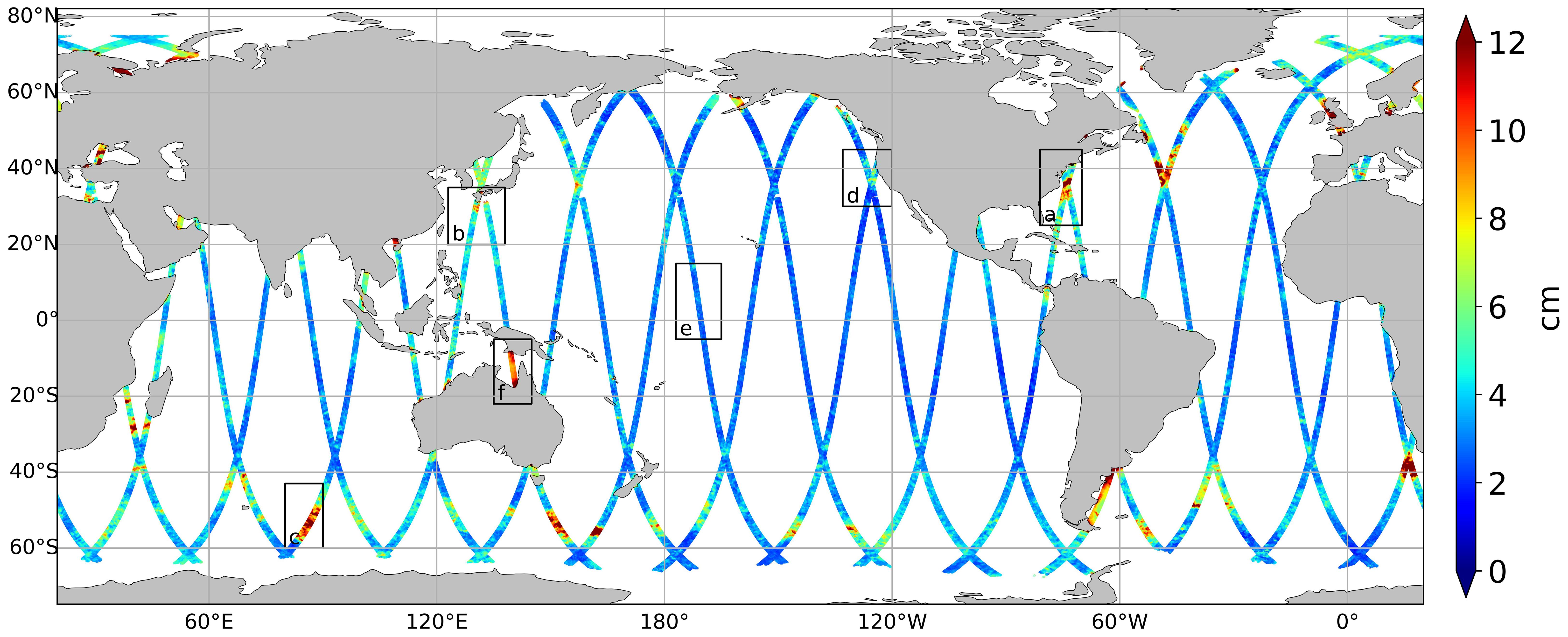
Figure 1. Global map of the root mean square of model misfits relative to SWOT SLA (in cm) over the period from March to July 2023. The boxes indicate the areas selected for regional analyses, see Figure 2.

The analyses presented in this study are based on SWOT Level-3 version 1.0, released on AVISO in May 2024. We use the ssha_noiseless variable (hereafter referred to as the sea level anomaly (SLA)) of the product, which consists of the SSH field denoised using U-net model (Treboutte et al., 2023) and Gomez algorithm (Gomez-Navarro et al., 2020). These filters reduce instrument random noise while preserving oceanic signals in SSH and its derivatives, allowing products to resolve ocean features as small as 10 km. The SLA measurements are corrected from the classical altimetric geophysical corrections, including barotropic and loading tides with the FES2022 model (Lyard et al., 2023; Carrère et al., 2023), internal tides using HRETv8.1 (Zaron, 2019), and the dynamic atmospheric correction (DAC) with the TUGO model. The findings of this study, including for internal tide residuals estimates, remain consistent and valid for SWOT version 2.0 (January 2025), which includes an updated internal tide correction from HRET8.1 and HRET14.SWOT observations undergo additional denoising through MOi assimilation system to align with the model horizontal resolution and optimize computational efficiency. SLA data are averaged and sub-sampled to reach a 6km x 6km resolution. This approach spatially smooths the SLA fields, filtering out the smallest features (as later illustrated in Section 3.2.2). Analyses have been conducted to confirm that the results obtained from such SWOT sub-sampled observations remain valid when applied to SWOT native 2-km grid. As no temporal filtering is applied, we ensure that time-based statistical metrics and frequency spectra of SLA time series remain unchanged.

2.2 Physical ocean model and assimilation system

SWOT SLA are compared with model simulations from GLO12V4, the MOi global forecasting system, which serves as the operational global component for real-time forecasting in the Copernicus Marine Service (Le Traon et al., 2021). This model uses the NEMO3.6 model (Nucleus for European Modelling of the Ocean, Madec et al., 2017) with a spatial resolution of 1/12° and a time step of 6 minutes. Tidal and atmospheric pressure forcings are not included in this simulation, and DAC is applied to align with the physical content of SWOT SLA. The full configuration of the system is detailed in Benkiran et al. (2021). The model analyses are generated using the SAM2 (Système d’Assimilation Mercator V2) data assimilation system described in Lellouche et al. (2018b) and Benkiran et al. (2021). In this configuration, the model assimilates SLA observations from nadir altimeters (Cryosat-2, HY-2B, Jason-3, Sentinel-3A & 3B, and Sentinel-6A), high-resolution Sea Surface Temperature (SST) data and in situ vertical profiles of temperature and salinity from the Copernicus SST and In Situ Thematic Assembly Centers (TACs). The model can dynamically propagate structures of five to nine grid cells, depending on the regional dynamics, we therefore expect to represent structures up to ~50 km.

The model outputs used in this study are computed at the exact same time and position as SWOT SLA observations.

2.3 Spectral methods

Frequency and wavenumber spectral densities allow quantifying the distribution of ocean energy across temporal and spatial scales. Conventional nadir altimetry missions, with their 10-day or longer sampling cycles, have provided valuable insights into the frequency characteristics of the ocean (Dufau et al., 2016; Ballarotta et al., 2019). The SWOT Cal/Val phase, with its daily sampling over a 3-month period, now enables the characterization of high-frequency ocean signals. However, because the spatial coverage during this phase is limited (approximately 9% of the global ocean), this study focuses on frequency analyses rather than spatial ones.

We employed the fast Fourier transform (FFT) with the Welch method (Welch, 1967) on SLA time series from SWOT observations and model outputs over the entire Cal/Val period (March 30, 2023, to July 9, 2023, spanning 100 days). This approach allows the generation of time series as long as possible which are needed to enhance the frequency resolution of the result. Only time series with at least 70% valid data were included in the spectral analysis to ensure consistency, and gaps in observations were filled via linear interpolation. This process eliminated time series with gaps longer than five consecutive days. We applied a linear detrending on SWOT and model time series and Tukey window of parameter 0.5. As density spectra can be sensitive to spectral computation parameters (Tchilibou et al., 2018), a series of sensitivity tests were conducted to confirm that the results were not influenced by artefacts of the spectral methods.

3 Results

The following sections provide an overview of the discrepancies between SWOT and the model equivalent SLA. The root mean square (RMS) of the differences displays misplaced or misshaped mesoscale features in the model, as well as submesoscale structures in SWOT SLA that are not resolved by the model. The frequency spectral analysis reveals differences in model and SWOT spectral slopes, as well as internal tide residuals in SWOT products.

3.1 Comparing SWOT and model SLA variability

The RMS of the differences between model equivalent SLA and SWOT SLA was computed over the Cal/Val period. RMS values were calculated only for time series with at least 70 days of valid data therefore regions with limited data, such as ice-covered areas (e.g., Hudson Bay and the Weddell Sea), do not appear in the analysis. The resulting RMS map is shown in Figure 1.

The discrepancies align closely with ocean dynamic patterns, with the highest misfit RMS values (over 10 cm) observed in regions of high ocean variability and intense eddy activity. These include major western boundary currents such as the Gulf Stream, the Agulhas Current and the Antarctic Circumpolar Current (ACC). The Kuroshio Current also exhibits notable discrepancies but with slightly lower RMS values compared to the Gulf Stream (~5 cm). Coastal shallow regions, including the Patagonian Shelf, the English Channel, the Irish Sea, and semi-enclosed seas like the Arafura Sea, also display large discrepancies between the model and SWOT SLA. Elsewhere, in regions with less dynamic variability, the agreement between SWOT and the model is generally better, although localized structures with small differences appear.

Figure 2 presents a focus on a selection of these key dynamic regions: the Gulf Stream, Kuroshio, South Indian Ocean, California Current, tropical Pacific, and Arafura Sea.

The Gulf Stream (Figure 2a) and Kuroshio (Figure 2b) are high-energy eddy regions characterized by large scale variability and sharp SLA gradients (Ma et al., 2016). While the largest structures observed by SWOT are captured by the model (nadir SLA and SST assimilation already constrains large scales), their precise location and shape may deviate, which explains the large differences values between model and SWOT variability. These large-scale differences also mask smaller discrepancies related to submesoscale features that are not represented in the model. As noted in Figure 1 and previously observed in Benkiran et al. (2021), the discrepancies appear to be more pronounced in the Gulf Stream than in the Kuroshio. The Agulhas Current (not shown) exhibits discrepancies on a similar scale to those in the Gulf Stream.

Figure 2

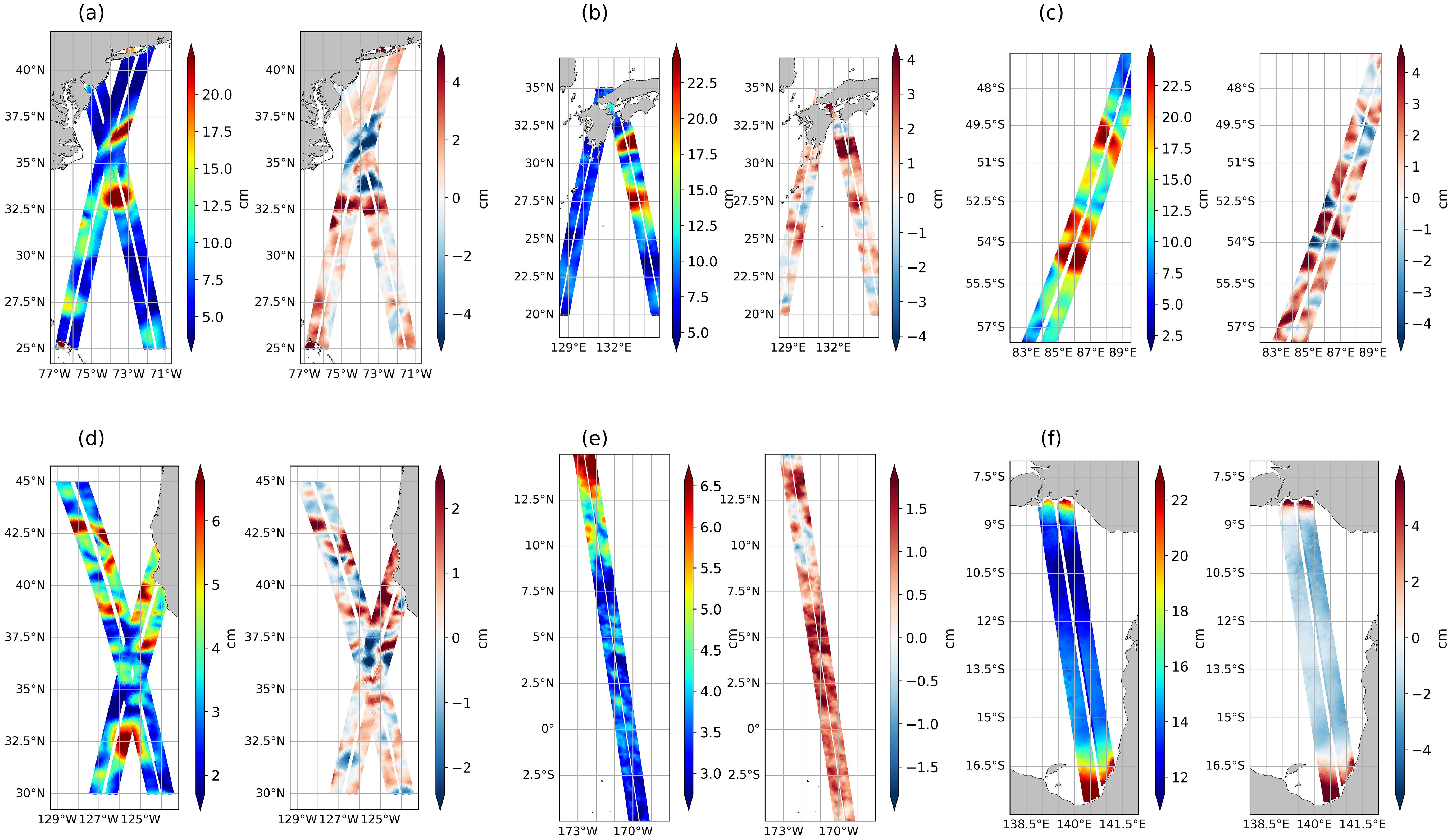
Figure 2. Maps of SLA variability from March to July 2023 in regions with different dynamical regimes : Gulf Stream (a), Kuroshio (b), South Indian Ocean (c), California Current (d), tropical Pacific (e), and Arafura Sea (f) ; see Figure 1 for locations.

The South Indian Ocean region (Figure 2c), as part of the ACC, is also a high eddy energy region subject to barotropic and baroclinic instabilities which generate smaller mesoscale eddies (Frenger et al., 2015). Such eddies are typically below the resolution of the nadir altimeters which constrain the model, but they can be observed by SWOT (Morrow et al., 2019).

The California Current (Figure 2d), as an eastern boundary current, shows less intense variability overall, yet SWOT SLA standard deviations reveal numerous small-scale structures as well, including meanders and filaments, that can be poorly resolved in the model.

The tropical Pacific (Figure 2e) is a region of active internal tide generation, where barotropic tidal currents interact with the complex bathymetry (Tchilibou et al., 2018). These rapid signals can be captured by SWOT (Fu et al., 2024) and significantly contribute to small-scale variability but are not included in the model’s physics, explaining the significant differences at these small scales.

Finally, the Arafura Sea (Figure 2f) and other semi-enclosed seas, such as the English Channel and the Irish Sea, also show high misfit RMS values. Unlike the other regions presented, the difference between SWOT and model variability does not exhibit eddy, front, or wave patterns but instead appears as a more homogeneous bias. This bias is most likely due to a misestimated mean dynamic topography (MDT) in the model equivalent computation of SLA (Eric Greiner, personal communication).

3.2 Frequency spectral analysis

3.2.1 Global frequency spectra

Oceans have been divided into 10°x 10° boxes to compare model and SWOT SLA frequency spectra. In each box, the spectral densities from time series of points below SWOT swaths have been averaged, both for SWOT and the model SLA. Figure 3 displays the resulting spectra. It provides a finer view of the temporal variability of the SLA, and a global view of temporal energy scales represented in the model and SWOT SLA. The y axes scales in the boxes change depending on the regions, to compare model and SWOT spectra shapes, thus spectral slopes cannot be quantified from this figure (see section 3.2.2 for spectral slopes analysis).

Figure 3

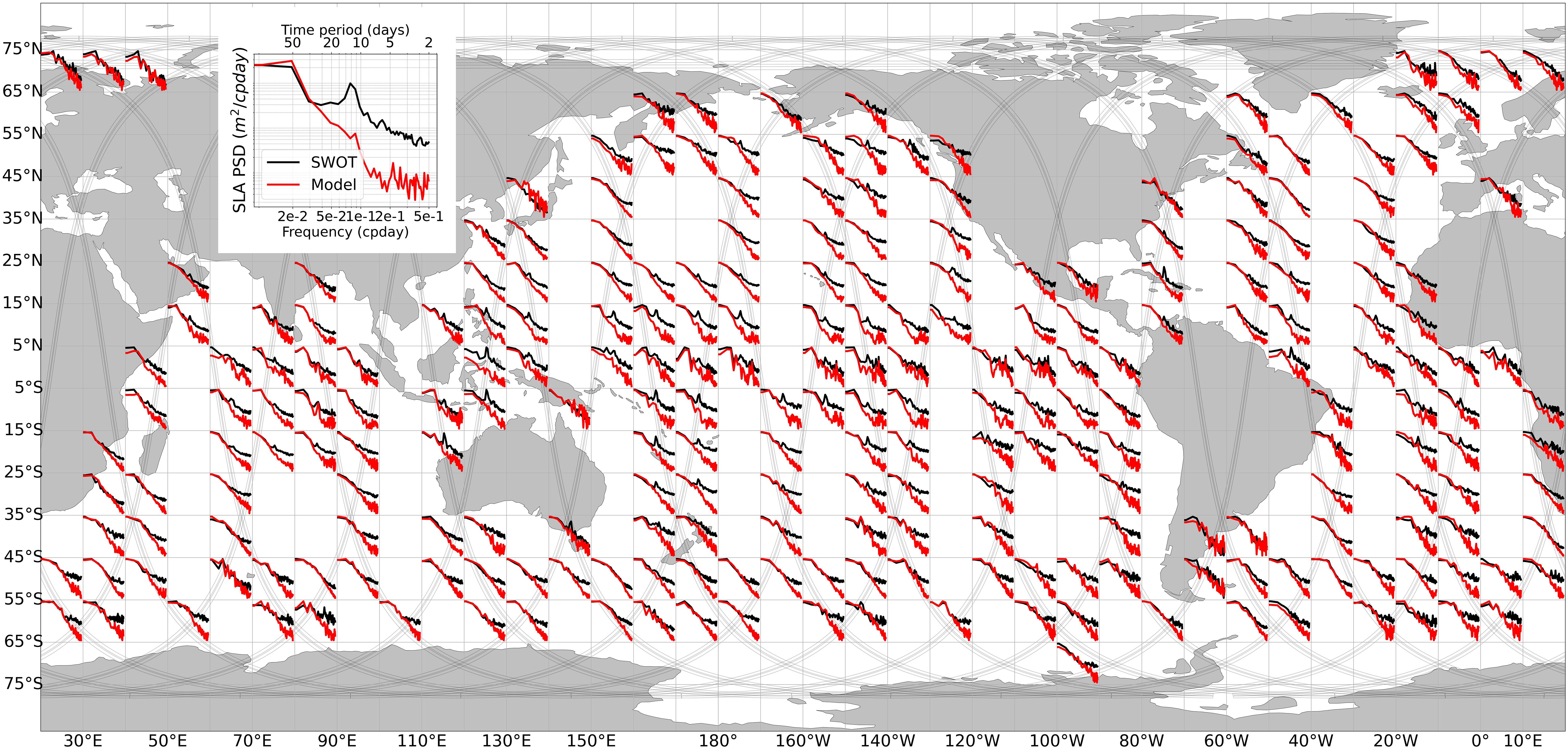
Figure 3. SLA frequency spectra (in m²/cpday) from SWOT data (black) and from the model outputs (red) globally averaged over 10°x10° grid boxes. Individual spectra were computed from 2023-03-30 to 2023-07-09 time series and averaged for each box. SWOT Cal/Val tracks are displayed in grey in the background.

The spectra show that SWOT and the model have consistent energy levels at larger time scales (over ~30 days), meaning that the dominant temporal mesoscale dynamics are accurately represented in the model. Largest and slowest structures are indeed already constrained by the assimilation of nadir altimeters and SST (Lellouche et al., 2018a). However, the model’s ability to represent the submesoscale high-frequency signals observed by SWOT varies depending on the regions. The energy levels diverge starting from frequencies ranging between 1/30 days and 1/10 days, with the model underestimating energy relative to SWOT observations. These high-frequency signals are typically linked to small-scale features that the model cannot resolve or may originate from residuals of geophysical corrections in SWOT SLA products. These points are further discussed in sections 3.2.2 and 3.2.3.

The agreement between SWOT and model spectra varies across regions. In extra-tropical dynamic regions like the Gulf Stream, Agulhas, and Kuroshio extensions, the spectra appear to be more aligned, as already noted in Biri et al. (2016), because mesoscale dynamics dominate (Storer et al., 2022). SWOT and model energy levels align well up to ~1/5-day frequencies in these extra-tropical regions: see North Atlantic boxes over 25°N for example. In contrast, spectra differ more significantly (from frequencies ~1/30 days) in the tropical band, where internal waves and tides play a more important role (Tchilibou et al., 2018): see Pacific boxes between -25°N and 25°N for example.

Finally, SWOT frequency spectra show remarkable energy peaks with a frequency of 1/12 days across several regions, primarily within the tropical band. These peaks are described and analyzed in section 3.2.3.

3.2.2 Spectral slopes

Spectra shown in Figure 3 highlight differences between model and SWOT frequency spectral slopes, which vary across frequency bands. Slopes are globally steeper over larger scales (1/50 to 1/10 days approximately) and flatten at smaller scales (<1/10 days), as previously observed in Biri et al. (2016) on the Atlantic using nadir altimeter data. The 1/20-day to 1/2-day frequency range is analyzed in this study to focus on the meso to submesoscales. To map spectral slopes within this band, we computed individual frequency spectra at each grid point, averaged them using a 1° rolling mean in latitude every 0.2°, and then derived spectral slopes for both SWOT and the model. Slopes are displayed in Figure 4, panel a and b respectively. SWOT shows steep frequency spectral slopes in highly dynamic regions (Gulf Stream, Kuroshio, Agulhas, ACC), with values ranging from f^−1.5 to f⁻³ and lower slopes elsewhere, around f0 to f⁻¹. Although the model follows the same general trend with steeper slopes in dynamic regions and aligns with SWOT slopes in the tropical band, its slopes are consistently steeper in extra-tropical regions, reaching values between f⁻³ and f⁻⁴. These model-derived slopes align with the estimates of Dufau et al. (2016), based on wavenumber spectral analysis of nadir altimeter data, close to k⁻⁴ in the main ocean currents and to k⁻¹ in the tropics. Qiu et al. (2017) attributes the observed flat slopes to mixed layer instability and unbalanced motions. Tchilibou et al. (2018) links the flat slopes to coherent and incoherent internal tides, along with non-tidal internal gravity waves.

Figure 4

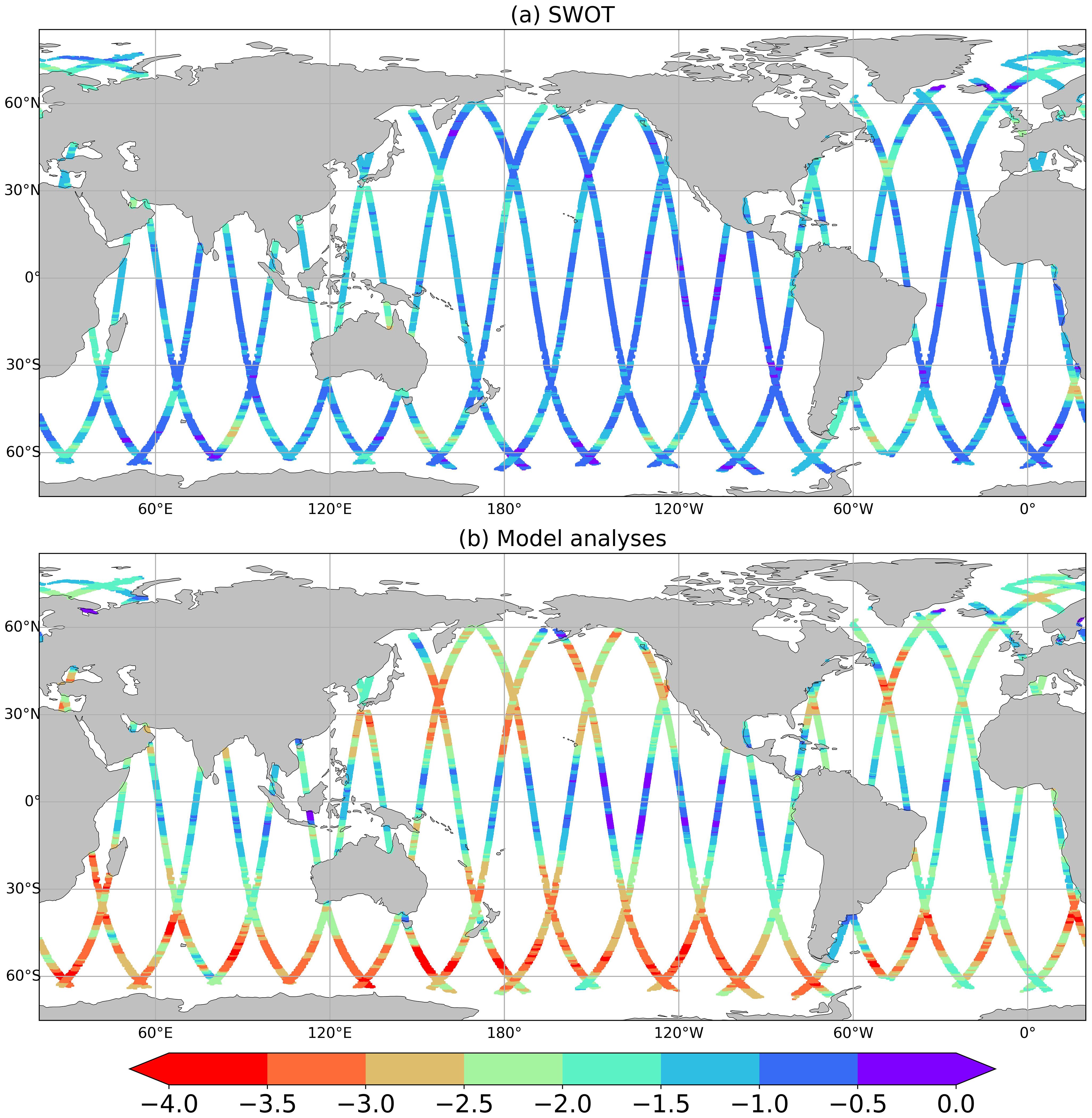
Figure 4. Spectral slopes estimated from mean SLA frequency spectra of SWOT (a) and model (b) over March–July 2023, in the frequency band 1/20 days to 1/2 days. Units: log(m²/cpday)/log(cpday).

To better understand the differences between the model and SWOT slopes in dynamic regions, the South Pacific Ocean was further analyzed. Figure 5 shows snapshot maps of the SLA as represented in SWOT products and in the model (panels a, b and c respectively), on 2023-04-18. This area is an ACC region where model and SWOT slopes diverge particularly. The maps show that SWOT observations (both original and sub-sampled data) contain variations at small spatial scales which are not represented in the model, whose SLA is much smoother due to the spatial resolution of its grid and its effective resolution. The figure also displays the time series of the SLA (panel d) in one point located by a cross on the map. It shows that this point has high-frequency variations that again, are not represented in the model. Similar analyses examining maps and time series were conducted in all regions where SWOT spectral slopes are flatter than those of the model. In every case, the results indicate that the slope differences stem from high-frequency signals in SWOT observations.

Figure 5

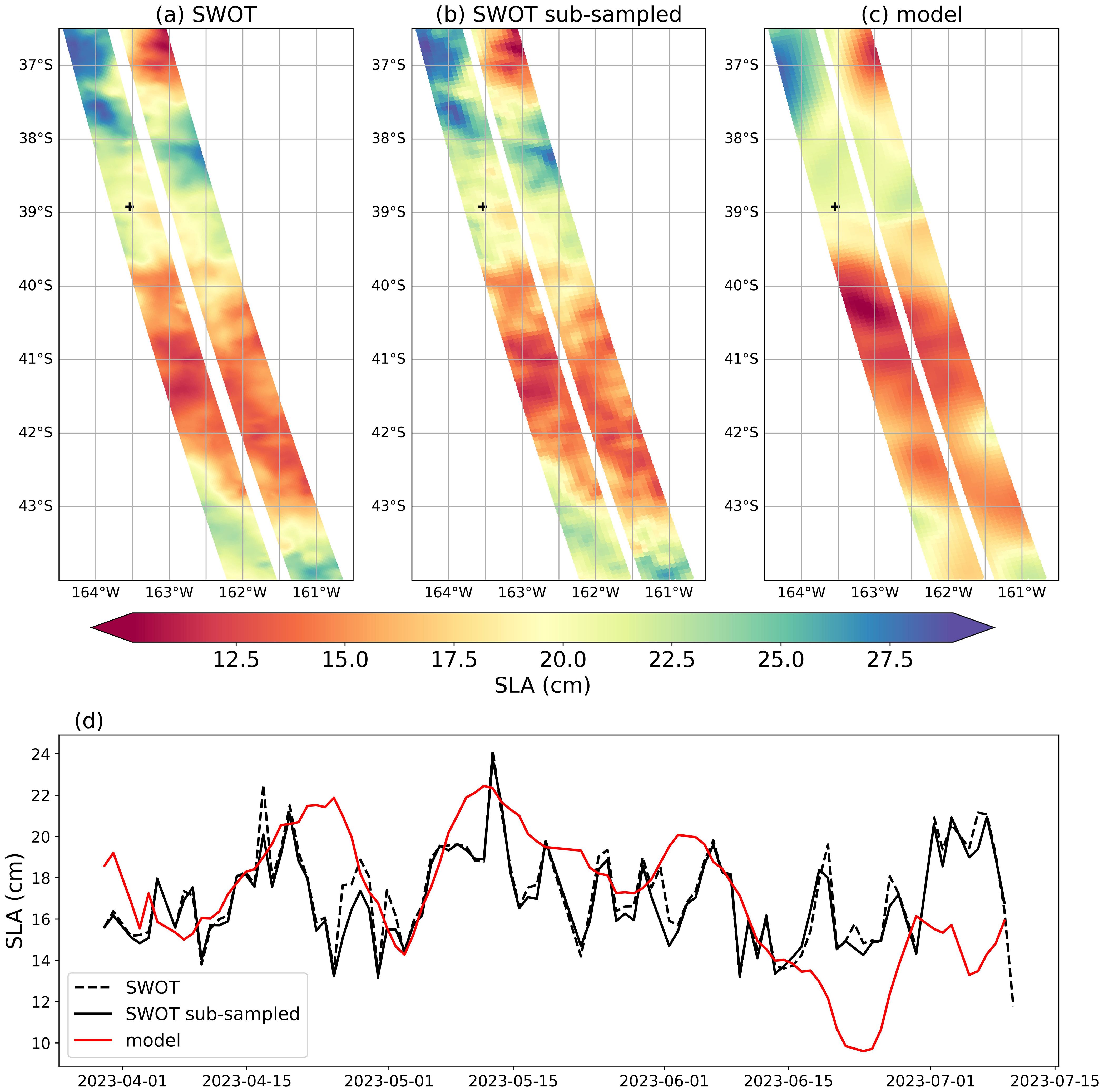
Figure 5. Snapshot of the SLA (cm) from SWOT original product (a), SWOT sub-sampled (b) and model analysis (c) along SWOT swath n.2 on 2023-04-18. SLA (cm) time series along SWOT Cal/Val phase of a point (d).

This suggests that the lower slopes in SWOT are driven by high-frequency, high-wavenumber ocean dynamics that the satellite captures but the model does not fully resolve. Such signal results from uncorrected or small signals that cannot be represented in the model, as observed in the tropical Pacific regional study (see section 3.2.3). The inconsistencies between the model and SWOT energy level at high frequencies can also be related to the 1/12° spatial resolution of the model which limits its capability to describe the small submesoscale signals which have a high-frequency signature.

3.2.3 Internal tide residuals

To better characterize the 1/12-day frequency energy peaks observed in Figure 3, wavenumber-frequency energy spectra from SWOT SLA were computed globally within 10°x10° boxes and compared to corresponding model spectra, along each SWOT swath. Figure 6a illustrates the spectra along SWOT swath n.28 in the Pacific Ocean, while Figures 6b, c provide a detailed view for the 45°–55°N box in SWOT and the model, respectively. Two distinct energy peaks (red stains in the spectra) are observed in Figure 6b, at a frequency of 1/12.4 days, corresponding to wavelengths of 171 km and 91 km. These peaks are not in the model spectra (Figure 6c), suggesting that the observed signals originate from geophysical processes captured by SWOT but not represented in the model.

Figure 6

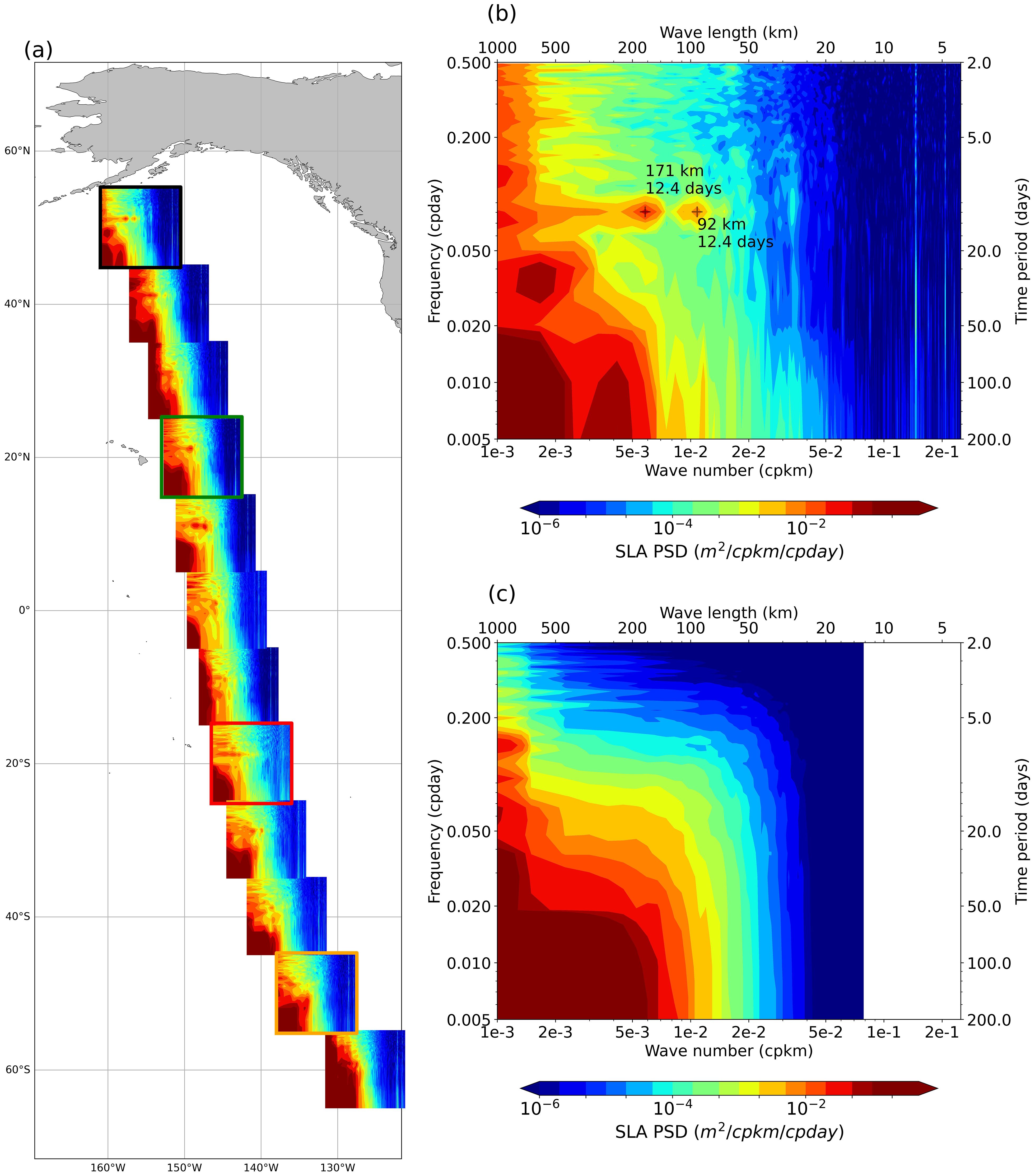
Figure 6. Wavenumber–frequency spectra of SWOT SLA along swath n.28 averaged in 10° latitude boxes (a). Boxes show spectral signatures of one (green) or two (black) coherent internal tide constituents, non-coherent tide signal (red) or no tide signal (orange). Zoom on black box for SWOT (b) and model (c). Units: m²/cpkm/cpday.

This signature aligns with tidal residuals. Specifically, the aliased frequencies of the M2 (12.42-hour period) and O1 (25.81-hour period) tidal components, when sampled at SWOT’s temporal resolution of 1/23.84 hours, are 1/12.32 days for M2 and 1/12.96 days for O1. Barotropic tidal corrections are highly accurate in the open ocean (Stammer et al., 2014; Lyard et al., 2023), suggesting that the observed residuals are most likely from baroclinic tides. The wavelengths identified are also consistent with Buijsman et al. (2020). Such internal tide signatures were already observed and analyzed in Dufau et al. (2016) with nadir altimeters in the same regions as the ones identified here.

Baroclinic tides comprise coherent, stationary components and incoherent, nonstationary ones. The coherent parts arise from the modulation of barotropic tidal currents by bathymetric gradients in a stratified ocean. They are typically concentrated near generation sites (see Appendix), they exhibit specific frequencies and wavenumbers, and they can be identified and corrected using harmonic analyses or models (Tchilibou et al., 2018). As coherent waves propagate through the ocean, interactions with mesoscale dynamics change them into incoherent tides, their spectral energy spreads across broader wavenumber and frequency bands, making them more difficult to isolate from other signals. Coherent internal tides are mitigated in SWOT SLA thanks to the HRETv8 model correction. Like other geophysical corrections in altimetry products, residuals may however remain. Residual aliased tidal signals were already detected in conventional nadir altimetry products (Zaron and Ray, 2018). Figure 6a illustrates the distinct characteristics of internal tide signals as viewed in SWOT along swath n.28.

In the black box, zoomed in Figure 6b, the two peaks at a frequency of 1/12.4 days indicate the presence of internal tides that remain phase-locked with tidal forcing. Such internal tides, coherent in time and in space, typically form near generation sites or in regions with weak mesoscale activity (Shriver et al., 2014). This signal could result from two distinct tidal constituents (M2 and O1) or from two different modes of a single tidal wave. Given that this box is located close to an M2 generation site but far from an O1 generation site (see Appendix), the two peaks are more likely associated with two modes of M2. In the green box, is located near both M2 and O1 generation sites, a single peak is observed. This suggests the presence of one mode from either of these tidal waves. The red box is located farther from internal tides generation sites. The spectrum shows an energy peak that is coherent in time (around the 1/12.4-day frequency), but that spreads uniformly across spatial scales from 100 to 1000 km. Such spatial scales do not correspond to coherent internal tides but are the manifestation of incoherent internal tide signal. Finally, the spectrum in the orange box displays no energy peak at the 1/12-day frequency, which indicates an absence of internal tide signals, whether coherent or incoherent.

Internal tide residuals, and unbalanced motions in general, should be removed from assimilation datasets because they are too fast to be properly captured by satellites with long revisit periods. Moreover, internal tides are not represented in the model, they should therefore be accounted for as ‘red’ noise in the assimilation system. Quantifying tidal residuals in SWOT SLA is therefore crucial for improving their assimilation.

To create a high-resolution global map of residuals in SWOT SLA at tidal frequencies, individual spectra were averaged within 1° latitude boxes at 0.2° intervals, and the standard deviation was calculated by integrating the excess spectral energy of the residual peak. The results, shown in Figure 7a, reveal standard deviations of approximately 1–2 cm in the tropical band, particularly in the western Pacific. Regions such as the Arafura Sea, Bass Strait, and areas near the Bahamas also show values exceeding 2 cm. These values are significant enough to affect the mesoscale representation in the assimilation system. However, in energetic regions like the Agulhas Current, the high standard deviation values may stem from other mesoscale signals than internal tides, with a frequency around 1/12 days as well. Ponte et al. (2017) propose using sea surface density observations to separate internal tides from mesoscale dynamics, since internal tides have a weaker impact on density. As SST maps fairly reflect surface density, analyzing their spectral content around the 1/12-day frequency could help provide a more detailed quantification of SWOT internal tide residuals. Figure 7b compares the standard deviations estimated here to the model misfit RMS shown in Figure 1, highlighting that tidal residual errors account for approximately 40% of the misfit RMS in tropical Pacific and Atlantic.

Figure 7

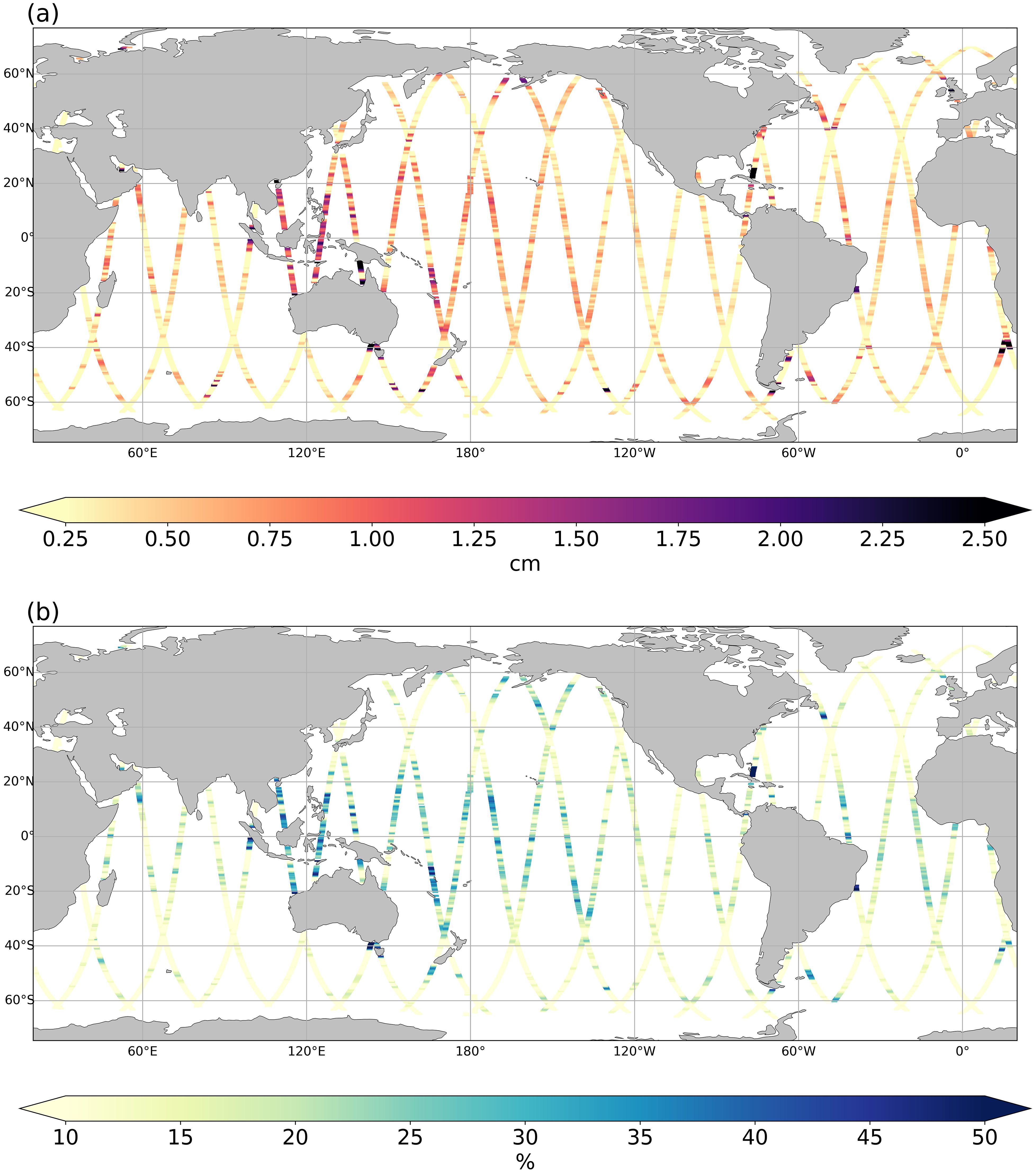
Figure 7. SLA standard deviation associated with the internal tide energy peak (a, in cm) and compared to the misfits RMS (see Figure 1) (b, in %). Individual spectra were averaged at 0.2° latitude intervals within 1° boxes. The spectral energy around the 1/12-day frequency peak was integrated and square-rooted to calculate the standard deviation.

4 Discussion and conclusion

This study has highlighted discrepancies between SWOT Cal/Val phase observations and SSH derived from a global high-resolution data assimilation system. Such a comparison is critical for successful assimilation of SWOT data in ocean models, which requires a detailed understanding of the signals captured in the observations.

Differences between SWOT and model SSH data are attributed to misplaced or distorted mesoscale features in the model and to submesoscale structures in SWOT SLA that nadir altimetry could not previously observe. From this Cal/Val phase analysis, we expect that assimilating SWOT data will improve the representation of mesoscale dynamics, refining the location and shape of the eddies already captured by the model and introducing smaller previously unresolved features.

The spectral analyses have also revealed both coherent and non-coherent internal tide residuals in the SLA, which are supposed to be corrected but may dominate the mesoscale and submesoscale signals in some regions. Such residuals were anticipated (Morrow et al., 2019) and have already been detected in SWOT measurements (Dibarboure et al., 2025). Continuous efforts are being made to improve internal tide models and altimetry corrections (Birol et al., 2025), leading to products with fewer geophysical residuals that will gradually become more reliable for data assimilation. However, some ocean signals, such as incoherent internal tides and solitons, cannot be fully corrected by models and Zaron (2015) estimates that at least 30% of internal tide sea level variations are incoherent.

These scales and processes are not represented by the model’s physics or are too small and too fast to be properly constrained by data assimilation. Because of the satellite revisit period (1 day for the SWOT Cal/Val phase, 21 days for the SWOT Science phase), their aliased signature can resemble balanced mesoscale signals and could add spurious energy to the system if assimilated. Continuously quantifying geophysical correction residuals is then crucial for estimating the representation error of SWOT observations (Oke and Sakov, 2008) and therefore minimizing these errors’ impact on assimilation.

In the first OSSE and OSE experiments conducted at MOi to assimilate SWOT observations, the observation error has been defined based solely on KaRIn instrument errors (Benkiran et al., 2021) and did not account for potential geophysical correction errors. To better estimate representativity errors, these errors will be updated by adding the internal tide residuals identified in this study. Moreover, the MOi assimilation system currently assumes a diagonal observation error covariance matrix, implying that observation errors are uncorrelated. However, SWOT observations exhibit strong spatial correlations (Dibarboure et al., 2025). Improving the characterization of observation errors should therefore also be considered to better assimilate SWOT observations.

This study paves the way for effectively integrating SWOT data into operational assimilation systems. Future studies will aim to evaluate how the assimilation system responds to SWOT high-resolution and high-frequency (Cal/Val phase) observations and how model’s performances depend on the model error characterization (incl. internal tides) as derived from this study.

Data availability statement

The raw data supporting the conclusions of this article will be made available by the authors, without undue reservation.

Author contributions

EF: Conceptualization, Formal Analysis, Methodology, Validation, Visualization, Writing – original draft, Writing – review & editing. MB: Data curation, Formal Analysis, Resources, Writing – review & editing. P-YL: Formal Analysis, Supervision, Writing – review & editing, Writing – original draft. ER: Formal Analysis, Writing – review & editing.

Funding

The author(s) declare that financial support was received for the research and/or publication of this article. This study was founded by CNES (French space agency) and Mercator Ocean International partnership agreement.

Acknowledgments

The HRETv8.1 products were obtained through personal communication with Ed Zaron. The authors thank Jérôme Chanut and Eric Greiner for their analyses and advice in this study. They also thank the three reviewers for their constructive comments and suggestions, which significantly added value to this paper. The SWOT_L3_LR_SSH product, derived from the L2 SWOT KaRIn low rate ocean data products (NASA/JPL and CNES), is produced and made freely available by AVISO and DUACS teams as part of the DESMOS Science Team project”. AVISO/DUACS 2024. SWOT Level-3 KaRIn Low Rate SSH Expert (v1.0) (CNES). doi: 10.24400/527896/A01-2023.018.

Conflict of interest

The authors declare that the research was conducted in the absence of any commercial or financial relationships that could be construed as a potential conflict of interest.

The author(s) declared that they were an editorial board member of Frontiers, at the time of submission. This had no impact on the peer review process and the final decision.

Generative AI statement

The author(s) declare that Generative AI was used in the creation of this manuscript.

This manuscript benefited from the use of generative AI tools for English language corrections (DeepL, ChatGPT).

Publisher’s note

All claims expressed in this article are solely those of the authors and do not necessarily represent those of their affiliated organizations, or those of the publisher, the editors and the reviewers. Any product that may be evaluated in this article, or claim that may be made by its manufacturer, is not guaranteed or endorsed by the publisher.

References

Archer M., Wang J., Klein P., Dibarboure G., and Fu L.-L.. (2025). Wide-swath satellite altimetry unveils global submesoscale ocean dynamics. Nature 640, 691–96. doi: 10.1038/s41586-025-08722-8

PubMed Abstract | Crossref Full Text | Google Scholar

Artana C., Provost C., Lellouche J. M., Rio M. H., Ferrari R., and Sennéchael N. (2019). The Malvinas current at the confluence with the Brazil current: inferences from 25 years of Mercator ocean reanalysis. J. Geophysical Res.: Oceans 124, 7178–7200. doi: 10.1029/2019jc015289

Crossref Full Text | Google Scholar

Ballarotta M., Ubelmann C., Pujol M.-I., Taburet G., Fournier F., Legeais J.-F., et al. (2019). On the resolutions of ocean altimetry maps. Ocean Sci. 15, 1091–1109. doi: 10.5194/os-15-1091-2019

Crossref Full Text | Google Scholar

Bell M. J., Schiller A., Le Traon P. Y., Smith N. R., Dombrowsky E., and Wilmer-Becker K. (2015). An introduction to GODAE oceanView. J. Operational Oceanogr. 8, s2–s11. doi: 10.1080/1755876X.2015.1022041

Crossref Full Text | Google Scholar

Benkiran M., Ruggiero G., Greiner E., Le Traon P.-Y., Rémy E., Lellouche J. M., et al. (2021). Assessing the impact of the assimilation of SWOT observations in a global high-resolution analysis and forecasting system part 1: methods. Front. Mar. Sci. 8. doi: 10.3389/fmars.2021.691955

Crossref Full Text | Google Scholar

Biri S., Serra N., Scharffenberg M. G., and Stammer D. (2016). Atlantic sea surface height and velocity spectra inferred from satellite altimetry and a hierarchy of numerical simulations. J. Geophysical Res.: Oceans 121, 4157–4177. doi: 10.1002/2015JC011503

Crossref Full Text | Google Scholar

Birol F., Bignalet-Cazalet F., Cancet M., Daguze J.-A., Fkaier W., Fouchet E., et al. (2025). Understanding uncertainties in the satellite altimeter measurement of coastal sea level: insights from a round-robin analysis. Ocean Sci. 21, 133–150. doi: 10.5194/os-21-133-2025

Crossref Full Text | Google Scholar

Buijsman M. C., Stephenson G. R., Ansong J. K., Arbic B. K., Green J. A. M., Richman J. G., et al. (2020). On the interplay between horizontal resolution and wave drag and their effect on tidal baroclinic mode waves in realistic global ocean simulations. Ocean Modelling 152, 101656. doi: 10.1016/j.ocemod.2020.101656

Crossref Full Text | Google Scholar

Carli E., Morrow R., Vergara O., Chevrier R., and Renault L. (2023). Ocean 2D eddy energy fluxes from small mesoscale processes with SWOT. Ocean Sci. 19, 1413–1435. doi: 10.5194/os-19-1413-2023

Crossref Full Text | Google Scholar

Carrère L., Lyard F., Cancet M., Allain D., Fouchet E., Dabat M.-L., et al. (2023). The new FES2022 Tidal atlas. Presented at the 2023 SWOT Science Team meeting (Toulouse). doi: 10.24400/527896/a03-2022.3287

Crossref Full Text | Google Scholar

Carrier M. J., Ngodock H. E., Smith S. R., Souopgui I., and Bartels B. (2016). Examining the potential impact of SWOT observations in an ocean analysis–forecasting system. Monthly Weather Review 144, 3767–82. doi: 10.1175/MWR-D-15-0361.1

Crossref Full Text | Google Scholar

Dibarboure G., Anadon C., Briol F., Cadier E., Chevrier R., Delepoulle A., et al. (2025). Blending 2D topography images from the Surface Water and Ocean Topography (SWOT) mission into the altimeter constellation with the Level-3 multi-mission Data Unification and Altimeter Combination System (DUACS). Ocean Sci. 21, 283–323. doi: 10.5194/os-21-283-2025

Crossref Full Text | Google Scholar

Dufau C., Orsztynowicz M., Dibarboure G., Morrow R., and Le Traon P.-Y. (2016). Mesoscale resolution capability of altimetry: Present and future. J. Geophysical Res.: Oceans 121, 4910–4927. doi: 10.1002/2015JC010904

Crossref Full Text | Google Scholar

Frenger I., Münnich M., Gruber N., and Knutti R. (2015). Southern Ocean eddy phenomenology. J. Geophysical Res.: Oceans 120, 7413–7449. doi: 10.1002/2015JC011047

Crossref Full Text | Google Scholar

Fu L.-L., Pavelsky T., Cretaux J.-F., Morrow R., Farrar J. T., Vaze P., et al. (2024). The surface water and ocean topography mission: A breakthrough in radar remote sensing of the ocean and land surface water. Geophysical Res. Lett. 51, e2023GL107652. doi: 10.1029/2023GL107652

Crossref Full Text | Google Scholar

Gómez-Navarro L., Cosme E., Sommer J. L., Papadakis N., and Pascual A. (2020). Development of an image de-noising method in preparation for the surface water and ocean topography satellite mission. Remote Sens. 12, 734. doi: 10.3390/rs12040734

Crossref Full Text | Google Scholar

Lellouche J.-M., Greiner E., Le Galloudec O., Garric G., Regnier C., Drevillon M., et al. (2018a). Recent updates to the Copernicus Marine Service global ocean monitoring and forecasting real-time 1/12° high-resolution system. Ocean Sci. 14, 1093–1126. doi: 10.5194/os-14-1093-2018

Crossref Full Text | Google Scholar

Lellouche J.-M., Greiner E., Le Galloudec O., Régnier C., Benkiran M., Testut C.-E., et al. (2018b). “The Mercator Ocean Global High-Resolution Monitoring and Forecasting System,” in New Frontiers in Operational Oceanography. GODAE OceanView. Eds. Chassignet E. P., Pascual A., Tintoré J., and Verron J. doi: 10.17125/gov2018.ch20

Crossref Full Text | Google Scholar

Le Traon P. Y., Dibarboure G., Jacobs G., Martin M., Remy E., and Schiller A. (2017). “Use of satellite altimetry for operational oceanography,” in Satellite Altimetry Over Oceans and Land Surfaces. Eds. Stammer D. and Cazenave A. (Boca Raton, FL:CRC Press).

Google Scholar

Le Traon P. Y., Abadie V., Ali A., Aouf L., Artioli Y., and Ascione I.. (2021). The Copernicus Marine Service from 2015 to 2021: six years of achievements. Special Issue Mercator Ocean J. 57. doi: 10.48670/moi-cafr-n813

Crossref Full Text | Google Scholar

Liu G., Smith G. C., Gauthier A.-A., Hébert-Pinard C., Perrie W., and Shehhi M. R. A. (2024). Assimilation of synthetic and real SWOT observations for the North Atlantic Ocean and Canadian east coast using the regional ice ocean prediction system. Front. Mar. Sci. 11. doi: 10.3389/fmars.2024.1456205

Crossref Full Text | Google Scholar

Lyard F., Carrere L., Dabat M.-L., Tchilibou M., Fouchet E., Faugere Y., et al. (2023). Barotropic correction for SWOT: FES2022 and DAC ». Oral présenté à SWOT-ST meeting, Toulouse. Available online at: https://swotst.aviso.altimetry.fr/fileadmin/user_upload/SWOTST2023/20230921_ocean_3_tides/11h00-2_FES2022-DAC.pdf. (Accessed May 05, 2025)

Google Scholar

Ma X., Jing Z., Chang P., Liu X., Montuoro R., Small R. J., et al. (2016). Western boundary currents regulated by interaction between ocean eddies and the atmosphere. Nature 535, 533–537. doi: 10.1038/nature18640

PubMed Abstract | Crossref Full Text | Google Scholar

Madec G., Bourdallé-Badie R., Bouttier P.-A., Bricaud C., Bruciaferri D., Calvert D., et al. (2017). NEMO ocean engine (Version v3.6), Notes Du Pôle De Modélisation De L’institut Pierre-simon Laplace (IPSL) (Zenodo). doi: 10.5281/zenodo.1472492

Crossref Full Text | Google Scholar

Morrow R., Fu L.-L., Ardhuin F., Benkiran M., Chapron B., Cosme E., et al. (2019). Global observations of fine-scale ocean surface topography with the surface water and ocean topography (SWOT) mission. Front. Mar. Sci. 6. doi: 10.3389/fmars.2019.00232

Crossref Full Text | Google Scholar

Oke P. R. and Sakov P. (2008). Representation error of oceanic observations for data assimilation. Journal of Atmospheric and Oceanic Technology 25, 1004–1017. doi: 10.1175/2007JTECHO558.1

Crossref Full Text | Google Scholar

Ponte A. L., Klein P., Dunphy M., and Gentil S. L. (2017). Low-mode internal tides and balanced dynamics disentanglement in altimetric observations: Synergy with surface density observations. Oceans 122, 2143–55. doi: 10.1002/2016JC012214

Crossref Full Text | Google Scholar

Qiu B., Nakano T., Chen S., and Klein P. (2017). Submesoscale transition from geostrophic flows to internal waves in the northwestern Pacific upper ocean. Nat. Commun. 8, 14055. doi: 10.1038/ncomms14055

PubMed Abstract | Crossref Full Text | Google Scholar

Shriver J. F., Richman J. G., and Arbic B. K. (2014). How stationary are the internal tides in a high-resolution global ocean circulation model? J. Geophysical Res.: Oceans 119, 2769–2787. doi: 10.1002/2013JC009423

Crossref Full Text | Google Scholar

Stammer D., Ray R. D., Andersen O. B., Arbic B. K., Bosch W., Carrère L., et al. (2014). Accuracy assessment of global barotropic ocean tide models. Rev. Geophysics 52, 243–282. doi: 10.1002/2014RG000450

Crossref Full Text | Google Scholar

Storer B.A., Buzzicotti M., Khatri H., Griffies S.M., and Aluie H. (2022). Global energy spectrum of the general oceanic circulation. Nat Commun 13, 5314. doi: 10.1038/s41467-022-33031-3

PubMed Abstract | Crossref Full Text | Google Scholar

Tchilibou M., Gourdeau L., Morrow R., Serazin G., Djath B., and Lyard F. (2018). Spectral signatures of the tropical Pacific dynamics from model and altimetry: a focus on the meso-/submesoscale range. Ocean Sci. 14, 1283–1301. doi: 10.5194/os-14-1283-2018

Crossref Full Text | Google Scholar

Tchonang B. C., Benkiran M., Le Traon P.-Y., Jan Van Gennip S., Lellouche J. M., and Ruggiero G. (2021). Assessing the impact of the assimilation of SWOT observations in a global high-resolution analysis and forecasting system – part 2: results. Front. In Marine Sci. 8. doi: 10.3389/fmars.2021.687414

Crossref Full Text | Google Scholar

Tréboutte A., Carli E., Ballarotta M., Carpentier B., Faugère Y., and Dibarboure G. (2023). KaRIn noise reduction using a convolutional neural network for the SWOT ocean products. Remote Sens. 15, 2183. doi: 10.3390/rs15082183

Crossref Full Text | Google Scholar

Welch P. (1967). The use of the fast Fourier transform for the estimation of power spectra: A method based on time averaging over short, modified periodograms. IEEE Trans. Audio Electroacoustics 15, 70–73. doi: 10.1109/TAU.1967.1161901

Crossref Full Text | Google Scholar

Zaron E. D. (2015). Nonstationary Internal Tides Observed Using Dual-Satellite Altimetry. Journal of Physical Oceanography 45>, 2239–46. doi: 10.1175/JPO-D-15-0020.1

Crossref Full Text | Google Scholar

Zaron E. D. (2019). Baroclinic tidal sea level from exact-repeat mission altimetry. Journal of Physical Oceanography 49>, 193–210. doi: 10.1175/JPO-D-18-0127.1

Crossref Full Text | Google Scholar

Zaron E. D. and Ray R. D. (2018). Aliased tidal variability in mesoscale sea level anomaly maps. doi: 10.1175/JTECH-D-18-0089.1

PubMed Abstract | Crossref Full Text | Google Scholar

5. Appendix A

Figure A1 displays M2 and O1 internal tide estimates as computed in HREV8.1, the correction used for SWOT SLA. It highlights the generation sites and regions where internal tide signals are expected.

Figure A1

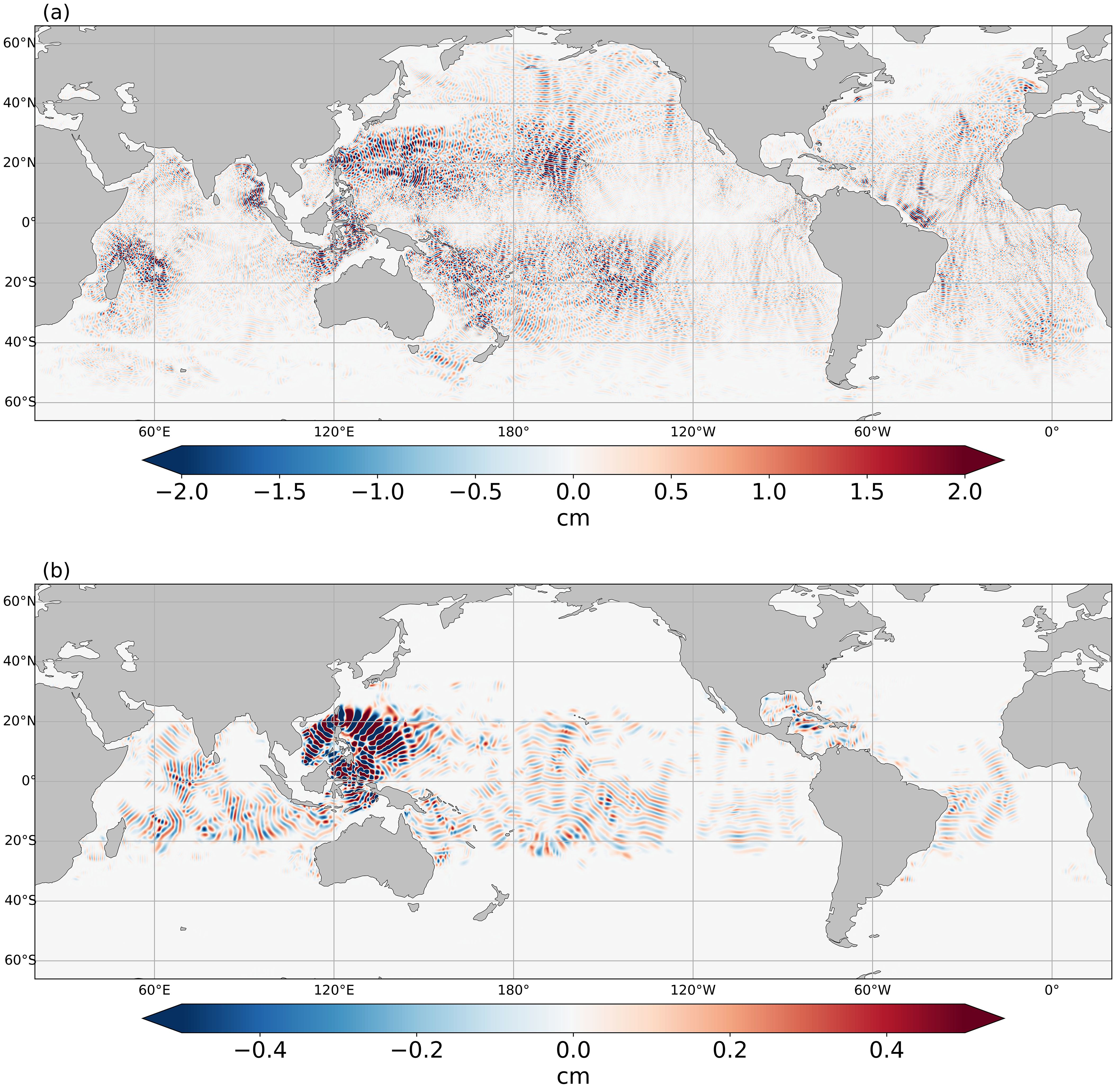
Figure A1. M2 (a) and O1 (b) baroclinic tide in-phase estimates from HRETv8.1 computed as described in Zaron (2019).