The role of sea surface circulation and weather dynamics in the PAH contamination in coastal mussels: a case study in the Southern Tyrrhenian sea

The Gulf of Pozzuoli, a marginal sub-basin of the Tyrrhenian Sea, has a longstanding tradition of bivalve mollusk farming. Despite its historical importance, the area faces significant anthropogenic pressures, particularly from the decommissioned industrial site at Bagnoli. Seasonal monitoring data indicate peaks in mussel contamination by polycyclic aromatic hydrocarbons (PAHs) in late autumn and early winter. This study analyzed the oceanographic and meteorological dynamics driving PAH contamination in 2016, when elevated PAH concentrations were recorded at one farming site. A combination of in situ measurements, satellite observations, numerical model outputs, and Lagrangian simulations was used to examine sea surface circulation, wind patterns, wave dynamics, and particle transport pathways. Contamination events were consistently preceded by approximately one week of northwestward surface currents, likely facilitating pollutant transport from Bagnoli to the farming area. Southerly waves exceeding 1.2 meters in height and periods longer than 8 seconds were recorded prior to contamination peaks, suggesting wave-induced resuspension of PAHs from sediments. These hydrodynamic conditions coincided with prevailing southwesterly winds. The findings support the hypothesis that specific meteorological and oceanographic conditions enhance PAH transport from Bagnoli to the mussel farms, posing risks to aquaculture and public health. Based on previous and current data, the study provides robust conclusions on PAH pollution in the Gulf of Pozzuoli and offers a rationale for improving monitoring and management strategies to mitigate contamination risks in vulnerable coastal areas.

1 Introduction

The Gulf of Pozzuoli (GoP) is a small bay located in the northwestern area of the Gulf of Naples (GoN) (Figures 1a, b) within the southern Tyrrhenian Sea (TYS). Connected to the GoN via a 2 km wide and 100 m deep passage (De Maio et al., 1982), despite its small extension, the GoP holds significant historical and contemporary importance. Since ancient Roman times, it has served as a pivotal harbor for naval activities and a primary hub for bivalve mollusk farming. In the last century, it has also accommodated large industrial facilities that used the sea for the transportation of materials, until the eventual establishment of the Napoli and Salerno harbors and the decommissioning of industrial operations in the 1980s. The adjacent GoN extends along the continental shelf of southern Italy, covering approximately 900 km² with an average depth of 170 m (Carrada et al., 1980). The region stretches southwestward towards the open sea. Spanning 195 km from the town of Monte di Procida to the promontory of Punta Campanella, the GoN physiographic unit includes the coastline from the town of Pozzuoli (Phlegraean coast) to the town of Sorrento. Water exchanges with the open sea are somewhat limited by the presence of Procida, Ischia, and Capri islands. The Campania region Coastal System (CCS, de Ruggiero et al., 2016; Figure 1a) hosts fragile ecosystems, including several marine protected areas, facing significant anthropogenic pressures. The presence of major urban centers (e.g. Naples and Salerno) adds to these challenges, highlighting the importance of sustainable management practices to mitigate environmental impacts.

Figure 1

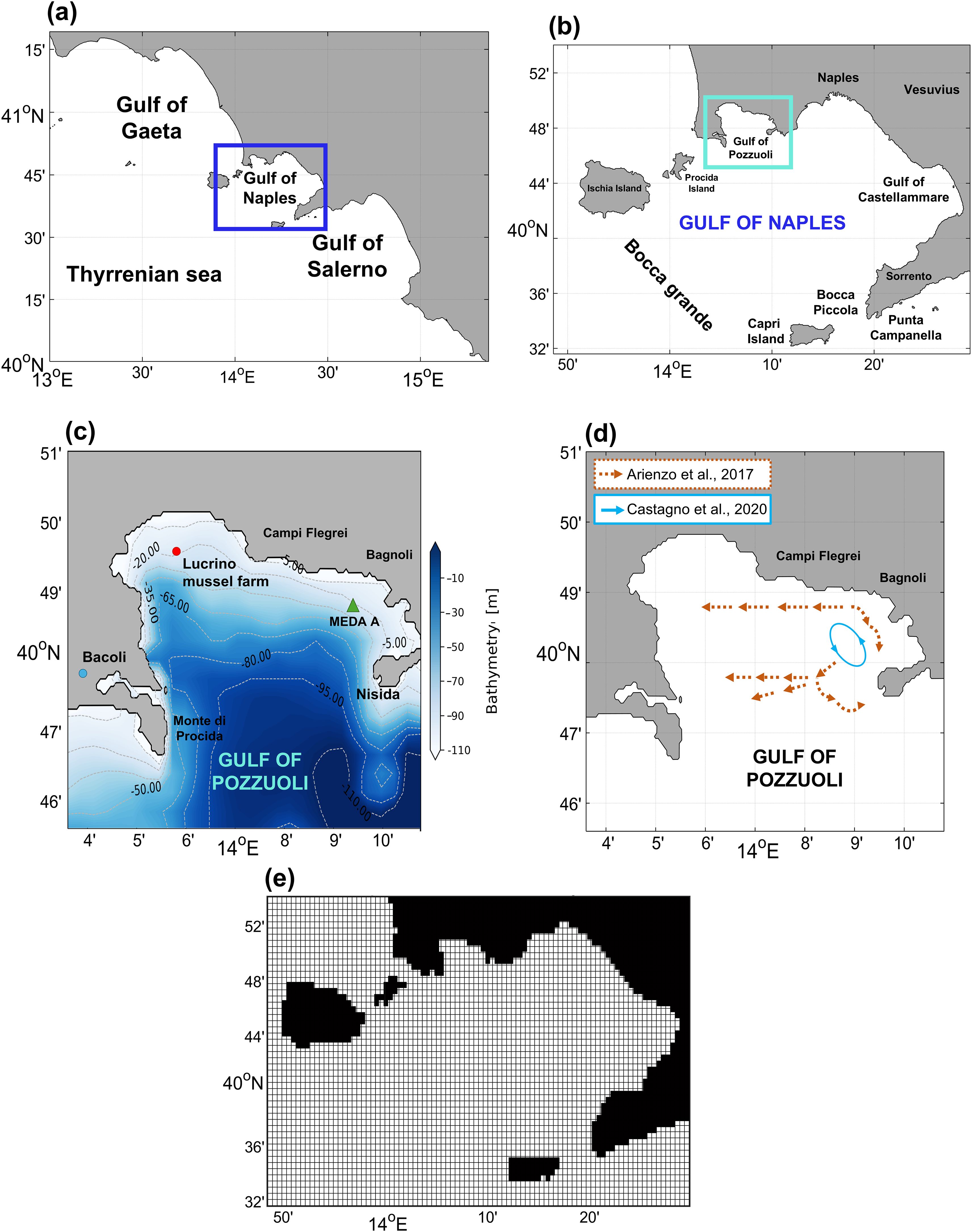
Figure 1. (a) Campania coastal system and CROM model domain (b) Zoom in the GoN (c) Bathymetric map of the GoP. The red dot corresponds to the position of the Lucrino mussel farm. The blue dot is the position of the Bacoli weather station. The green triangle is the position of MEDA A (d) Schematic sediment transport (orange – Arienzo et al., 2017) and sea surface circulation (lightblue – Castagno et al., 2020) at the Bagnoli Bay from previous studies; (e) Computational grid of the CROM model in the GoN.

In the GoP, a floating row system is used to farm bivalve mollusks, with a predominant focus on the high production and trade of the Mytilus galloprovincialis species. Thanks to their filtration-based feeding mechanism, mussels efficiently accumulate and concentrate substances dissolved in water in their tissue, including contaminants (Vaezzadeh et al., 2017). This makes them excellent bioindicators for assessing environmental pollution. Nevertheless, for food safety purposes, mussels intended for human consumption undergo systematic monitoring by health authorities to ensure that the levels of pollutants are lower than the limits set by legislation.

Polycyclic Aromatic Hydrocarbons (PAHs) are widespread environmental contaminants (Rubailo and Oberenko, 2008), primarily generated by the incomplete combustion of organic materials and industrial processes (Murphy and Morrison, 2002). In the Gulf of Pozzuoli, PAHs are mainly introduced through maritime traffic, port activities, shipbuilding and maintenance, industrial emissions, and urban discharges, all contributing to the contamination of marine sediments (Bjørseth and Ramdahl, 1985).

PAHs can easily bioaccumulate in organisms and can concentrate within various environmental matrices (Abdel-Shafy and Mansour, 2016; Oliva et al., 2020; Srogi, 2007) due to their low water solubility, low volatility, and high octanol/water partition coefficients (Sverdrup et al., 2002). While hundreds of PAH compounds exist in the environment, in the 1970s, the United States Environmental Protection Agency (USEPA) designated 16 unsubstituted PAHs as priority pollutants due to their elevated toxicity (Baumard et al., 1997; Srogi, 2007; Wise et al., 2015). In 2005, the European Community (EC) established a list of 15 + 1 priority PAHs, primarily in response to food-contamination issues, which included 8 PAHs from the USEPA list (Wenzl et al., 2006). Benzo(a)pyrene (BaP), classified by the International Agency for Research on Cancer (IARC) as carcinogenic to humans (Group 1, IARC classification (IARC, 2010), exemplifies the toxic potential of certain PAHs, with others recognized as probable (2A) or possible (2B) carcinogenic to humans, based on demonstrated synergistic actions.

In marine environments, PAHs originate from atmospheric deposition, contaminated sediments, industrial discharges, urban runoff, wastewater, and fossil fuel-related accidents (Douben, 2003; Yim et al., 2005). The contribution of atmospheric PAHs to aquatic environments is influenced by several factors, including precipitation, wind direction, and intensity, which can transport contaminated sediments to seawater, contributing to pollution (Guigue et al., 2017; Csanady, 1973; Lipiatou et al., 1993). Seasonal variations in solar radiation also play a role in the degradation of PAHs, with ultraviolet light absorbed by the upper water layer significantly contributing to their breakdown (Mill et al., 1981; Zhang and Tao, 2008). Due to their hydrophobic nature, PAHs readily bind to suspended particles and accumulate in sediments, where they persist longer than in the water column (Readman et al., 1984; Masood et al., 2018; Cerniglia and Heitkamp, 1989). Under certain conditions, such as changes in water temperature or current patterns, these compounds can be remobilized, becoming bioavailable once again (Sun et al., 2018). Additionally, phytoplankton and zooplankton contribute to the PAH levels in the water column, as they can carry hydrophobic compounds within their bodies and fecal pellets (Kowalewska and Konat, 1997; Prahl and Carpenter, 1979). PAHs are known for their slow biodegradation, and they tend to accumulate in the fatty tissues of organisms, posing significant health risks through trophic transfer, particularly via seafood consumption (Binelli and Provini, 2003; Martorell et al., 2010; Kronenberg et al., 2017). To mitigate these risks, the European Union has established maximum limits for PAHs in food products. The first regulation, Commission Regulation (EC) No 1881/2006 (Commission Regulation (EU) 1881/2006, 2006), set maximum limits for PAHs in food, which was later amended in 2011 by Regulation EU 835/2011, identifying benzo(a)pyrene (BaP), benz(a)anthracene (B(a)A), benzo(b)fluoranthene (BbF), and chrysene (CHR) as indicators for the presence of 16 EU priority PAHs. Furthermore, Regulation EU 2023/915 established specific maximum limits for PAHs in bivalve mollusks as food products, including 5.0 µg/kg for BaP individually and 30.0 µg/kg for the sum of BaP, BaA, BbF, and CHR. BaP is used as an environmental risk indicator due to its stability in the environment and significant carcinogenic potential, which poses a serious threat to living organisms and is a primary concern in seafood safety.

This study investigates the high pollution events in mussels farmed in the Lucrino site of the GoP recorded during 2016 when greater availability of in situ data and validated model outputs (Gifuni et al., 2022) are available for this small area. Sea and weather conditions and dynamics are discussed through the analysis of available in situ oceanic and atmospheric data, as well as through outputs from a high-resolution circulation model tailored to the region (de Ruggiero et al., 2016, 2020).

The primary aim of this paper is to identify and examine potential oceanic and atmospheric circulation patterns associated with contamination episodes, with the final goal of providing a comprehensive understanding of the abiotic factors influencing mussel farming activities. These findings could be integrated into a broader forecasting framework aimed at supporting local governments and farmers in predicting pollution events, building upon recent advancements in this field (Montella et al., 2020).

The paper is organized as follows. In the “Materials and Methods” section, we provide a detailed overview of the study area, the methodology employed for measuring PAH concentrations and the meteo-marine data utilized for environmental analysis. In the “Results” section, we present an analysis of in situ data for each pollution event, alongside scenarios derived from simulations of transport driven by sea surface currents. In the “Discussion” section, we interpret the findings in the context of environmental dynamics and pollutant transport mechanisms. Finally, in the “Conclusions” section, we summarize the key findings and their implications for monitoring and management strategies.

2 Materials and methods

2.1 Study area

The GoP extends from Nisida island to Bacoli town, covering an area of approximately 33 km² in the northwest part of the GoN (Figure 1c), with an average depth of about 60 m and a maximum depth of 110 m (Somma et al., 2016). The bay is positioned within the tectonic system of Campi Flegrei and it defines the northern boundary of a volcanic caldera. Its geology is characterized by dynamic features due to ongoing volcanic activity, as evidenced by submarine gas emissions and bradyseismic movements. Additionally, human activities have contributed to the degradation of both the natural landscape and the archaeological heritage of this valuable area. Notably, in 1854, the first chemical production plant was built in Bagnoli (Figure 1c). By the early 1900s, the area had developed as a focal point for industrialization in Italy, causing the establishment of large-scale industrial facilities engaged in several activities, ranging from steel production to cement and asbestos manufacturing. The obvious environmental hazards posed by industrial activities in the Bagnoli site led to a decommissioning phase for the entire industrial complex, which had become the second-largest integrated steel plant in Italy. Steel production ceased definitively in 1990, and the industrial facilities were completely dismantled in the early 2000s (Romano et al., 2004).

Presently, this area is undergoing remediation through a government project. The remediation efforts started in 1996 and were extended to include the marine sediments along the coastal area adjacent to the brownfield site in 2001 (Albanese et al., 2010). The long industrial activity spanning decades has caused serious environmental damages that persist. Additionally, the intense maritime traffic associated with port and industrial operations has contributed to marine pollution. The extent of environmental degradation is significant, prompting rising concerns about the spread of contamination throughout the entire GoP (Armiento et al., 2020).

2.1.1 Marine dynamics of the Gulf of Naples and the Gulf of Pozzuoli

Previous studies have attempted to delineate oceanic circulation patterns in the GoP to better understand the distribution and fate of contaminated sediments (Bonamano et al., 2021; Arienzo et al., 2017).

Nevertheless, as the GoP is part of the larger GoN, interactions between their circulation patterns may occur. Within the CCS, the GoN is likely the region most impacted by human activities, placing significant pressure on its marine ecosystem (Buonocore et al., 2010). These activities range from extensive urban development and intensive tourism to industrial zones lining the coast, leading to the potential discharge of sewage, industrial effluents, and hydrocarbons (Tornero and Ribera d’Alcalà, 2014). Moreover, the GoN serves as a vital hub in the Mediterranean for both touristic and commercial marine traffic (De Pippo et al., 2008). Furthermore, the complex local oceanic circulation amplifies the effects of human activities on the marine environment, facilitating the dispersal of marine litter and pollutants originating from coastal sources, thereby posing an additional threat to the fragile local ecosystems (Iacono et al., 2021; Gifuni et al., 2023; Cesarano et al., 2023). Water circulation within the GoN is closely linked to the local wind regime and/or to the large-scale flow of the TYS (Carrada et al., 1980). Although traditionally described as a large cyclonic motion (Millot, 1999), circulation within the TYS is highly complex and presents pronounced seasonal variability (e.g., Rinaldi et al., 2010; Krauzig et al., 2020; Iacono et al., 2021).

Various remote and local factors influence circulation within the GoN (see Figure 2). The primary remote forcing is attributed to the southern TYS, as its circulation patterns play a significant role in steering water mass movements within the basin (Gravili et al., 2001; Pierini and Simioli, 1998). On the other hand, wind is the main driver of sea surface dynamics, exhibiting the highest spatial and temporal variability (Moretti et al., 1976-1977; De Maio et al., 1985; Menna et al., 2007).

Figure 2

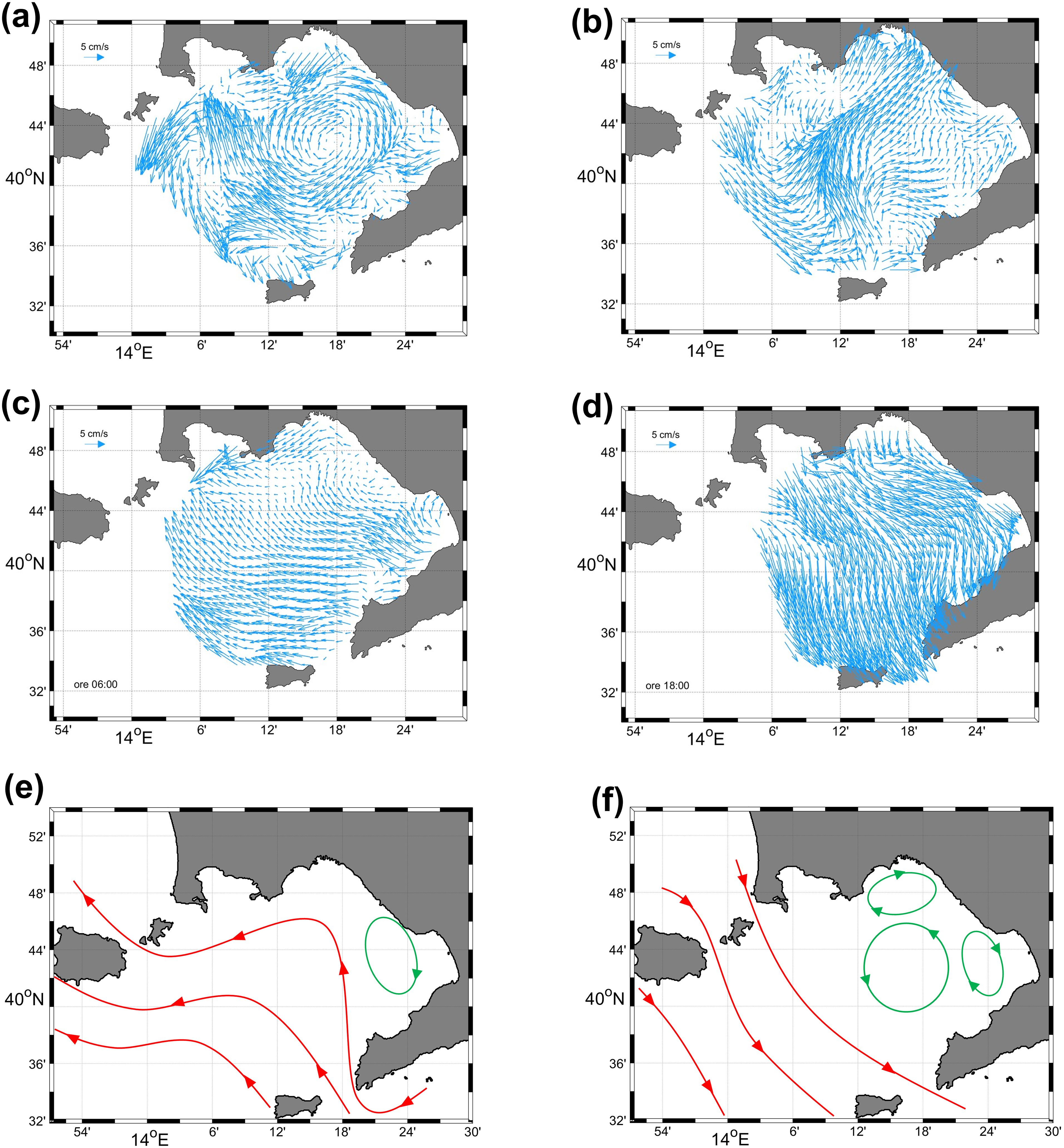
Figure 2. (a) Sea surface circulation in the GoN detected by HF radar measurements during NE wind; (b) Sea surface circulation in the GoN detected by HF radar measurements during SW wind; (c, d) Sea surface circulation in the GoN detected by HF radar measurements during the daily alternation of breeze winds. The two maps show the circulation fiel: at 06:00 GMT (c) when the flow is mainly directed offshore; at 18:00 GMT (d) when the flow is reversed; (e) Schematic circulation in the GoN as driven by north-westward Tyrrhenian current (red curve line). The green circle is the anticyclonic structure (modified from De Maio et al., 1983); (f) Schematic circulation in the GoN as driven by a south-eastern Tyrrhenian current (red curve line). The green circles are the anticyclonic and cyclonic structure (modified from De Maio et al., 1983).

The basin-scale circulation often shows complex patterns, including cyclonic and anticyclonic vortices, jet streams, convergence and divergence zones, and other oceanic structures (Cianelli et al., 2011). To describe this circulation, we present (Figure 2) a set of four sea surface circulation patterns observed by a CODAR HF (High-Frequency Coastal Ocean Dynamics Applications Radar) radar system in the GoN since October 2004. This system enables real-time, synoptic monitoring of the surface current field at the basin scale. The CODAR system is managed by the Università degli Studi di Napoli “Parthenope” on behalf of the Centre for the Analysis and Monitoring of Environmental Risk (see Menna et al., 2007; Cianelli et al., 2011 for further details). Over the years, the observations accumulated have also received strong feedback by modelling results (Gravili et al., 2001; Grieco et al., 2005) leading to a better understanding of the basin’s circulation dynamics.

As reported by Menna et al. (2007), during winter prevailing winds typically blow from the NNE-NE direction, with speeds reaching 8–10 m/s and occasional gusts from the SW exceeding 10 m/s. Under these conditions, an offshore-directed jet current is observed, as illustrated in Figure 2a. Conversely, when winds blow from the SW, currents predominantly flow towards the inner part of the basin, as depicted in Figure 2b.

During spring and summer, atmospheric conditions are characterized by alternating NE and SW winds, with a dominant breeze regime (Perusini et al., 1992; Menna et al., 2007; Cianelli et al., 2011), resulting in a daily alternation between sea and land breezes. In response, the GoN is characterized by a synchronous clockwise rotation of the surface current field, as shown in Figure 2c, d.

When the remote forcing of the TYS circulation is dominant, two divergent scenarios can be outlined (De Maio et al., 1982; De Maio et al., 1983; de Ruggiero, 2013). When the primary coastal current of the TYS flows northwestward (Figure 2e), an intense flow enters the GoN from the Bocca Piccola, nearly parallel to the Bocca Grande, and moves toward the island of Ischia. At the basin scale, a cyclonic vortex prevails, while an anticyclonic structure forms in the Gulf of the town of Castellammare di Stabia (in the southeastern part of the GoN). This pattern is most observed during winter and autumn (de Ruggiero et al., 2020). By late spring, circulation within the GoN intensifies, with surface currents reaching up to 20 cm/s, fostering an anticyclonic pattern across the entire coastal area of the GoN, except in the GoP sector. In late spring, circulation within the GoN intensifies, producing surface currents of up to 20 cm/s and an anticyclonic pattern across the entire coastal region, except in the GoP sector.

When the Tyrrhenian coastal current shifts southeastward (Figure 2f), the surface circulation pattern in the outer GoN shows a cyclonic structure, while prominent anticyclonic gyres form in the Bay of Naples (situated in the northeastern sector of the basin) and the Gulf of Castellammare di Stabia (de Ruggiero et al., 2020).

In this broader dynamic context, the GoP emerges as a semi-enclosed sub-basin whose circulation patterns are less understood due to limited in situ data at the basin scale. Recently, hydrographic measurements and numerical modeling (Castagno et al., 2020) have been used to analyze water mass properties, providing insights into the variability of the eastern GoP. Their findings reveal the presence of a persistent anticyclonic (clockwise) circulation system (Figure 1d) driven by local wind stress curl, with a lesser influence from the large-scale forcings.

In the GoP, sedimentary dynamics are largely driven by granulometric subpopulations, with fine and very fine sands playing a key role (Arienzo et al., 2017; Figure 1d). Fine sand is generally mobilized by a westward longshore current in shallow nearshore waters (depths <10 m) and by a cyclonic (anticlockwise) circulation between Bagnoli Bay and the GoP, while very fine sand tends to follow an offshore east–west transit axis relative to the Bagnoli brownfield site (Figure 1d, Arienzo et al., 2017). This dynamic sedimentary regime contributes to the redistribution of contaminants originating from local sources. In particular, elevated concentrations of PAHs in both surface and bottom sediments have been documented near the Bagnoli site (Tornero and Ribera d’Alcalà, 2014; Qu et al., 2018), and monitoring data from shellfish production in the GoN identified the nearby Lucrino site as showing the highest frequency of samples exceeding regulatory limits for both BaP and total PAHs, with a clear seasonal pattern (Esposito et al., 2017; 2020). Additional studies on marine sediments (Albanese et al., 2010; Bergamin et al., 2003; Romano et al., 2004; Arienzo et al., 2020) confirmed widespread contamination by heavy metals, PAHs, polychlorinated biphenyls (PCBs), and total hydrocarbons (HC) in proximity to Bagnoli. While high levels of PAHs and PCBs have been attributed to past industrial activities (Albanese et al., 2010), the elevated concentrations of heavy metals are mainly linked to natural hydrothermal enrichment processes associated with the volcanic activity of the Campi Flegrei caldera.

2.2 PAH concentration in farmed mussels

Coastal ecosystems, recognized for their vulnerability to pollutant accumulation, particularly highlight PAHs as the primary class of pollutants (Akinsanya et al., 2018; Sharifi et al., 2022). Given the paramount importance of protecting public health, maintaining pollutants at acceptable levels in mollusks is a top priority. Campania Region coastal farms are regularly subjected to chemical monitoring to assess the concentration of four PAHs in the soft tissue of mussels (Mytilus galloprovincialis).

Monitoring in the farming sites is carried on using the method described by Esposito et al. (2017) for the determination of PAHs concentration. In particular, mussel samples were collected by authorized personnel at the shellfish farming plants, constituting a pool of approximately 1 kg of commercial-sized specimens. Mussels were randomly collected along the longline, which extends approximately 3–4 meters below the surface, ensuring a representative sampling across different depths. Then, samples from farms located in the Lucrino site of the Gulf of Pozzuoli are transferred on ice to the Istituto Zooprofilattico Sperimentale del Mezzogiorno (IZSM) laboratories, where they were dissected. Sampled mussels were selected and characterized by similar maximum valve length (5–7 cm), weight (3–5 g) and age (9–11 months old). Soft tissue from 20 to 40 specimens were individually wrapped in aluminium foil and stored at −20°C until analysis performed after 5–6 days. The analyses were performed using a HPLC method developed by Serpe et al. (2010), in compliance with the Regulation EU 836/2011 (Commission Regulation EU 836/2011, 2011; Commission Regulation (EU)835/2011, 2011) that does not require analyses on water or sediment samples but only in the final edible product (i.e., mussel tissues), nor separate sampling at different depths or the analysis of interstitial water samples for food safety purposes.

The procedure involved homogenizing mussel tissues, saponification, extraction with cyclohexane, and purification using Sep-Pak silica cartridges. Extracts were analyzed by HPLC using a specific column and gradient elution program with an acetonitrile/water mobile phase. PAH peaks were identified by comparing retention times with standards, and concentrations were determined using an external standard method. The method was fully validated, with a quantification limit of 0.2 μg/kg and recoveries ranging from 50% to 120%, as required by EU regulations.

2.3 Meteorological data

Wind speed and direction data are used in this study to describe the local atmospheric forcing on ocean circulation in the GoP area. These data have been collected by the Bacoli weather station (blue dot in Figure 1c) and made available through the Campanialive network (https://www.campanialive.it/). Bacoli weather station collects the following values: temperature, humidity, heat index, sea-level pressure, wind, and ultraviolet (UV) radiation index. This station, located in the western part of the GoP (40° 47’ 31.38’’ N, 14° 4’ 40.11’’ E) at 3 m above sea level, provides weather data at 10-minute intervals and is the only station in the area that operated continuously throughout 2016. Additionally, the synoptic meteorological conditions during the pollution events of 2016 have been described using the NCEP Climate Forecast System Reanalysis, with a spatial resolution of 0.5° × 0.5°. Finally, in situ rainfall data from two automatic weather stations, located in Pozzuoli and Nisida island, have been analyzed to investigate the potential role of rain as a source of PAHs in the GoP.

2.4 In situ oceanographic data

In situ oceanographic data gathered by the “MEDA A” platform have been used to characterize water mass properties and dynamics along the coastal region of the GoP. This platform is managed by the Anton Dohrn Zoological Station of Naples (SZN). It is located in the bay of Bagnoli (40° 48.550’ N, 014° 09.300’ E) on a seabed of approximately 19 m depth (Figure1c). The “MEDA A” consists of an elastic beacon equipped with automatic instruments for continuous acquisition of meteorological and seawater parameters and dynamics. Data are transmitted to the ground station in real-time using both a broadband Wi-Fi bridge and the GSM network. Instruments on the elastic beacon include an automatic weather station, a multiparametric profiling probe, and an acoustic doppler current profiler. Given the limited completeness of the ‘MEDA A’ dataset, data from the Bacoli weather station were used as a substitute. For water column data, all available records from 1st January 2016 to 6th December 2016 have been used. Sea current data were acquired by an upward-looking 600 kHz Acoustic Doppler Current Profiler (ADCP), positioned on the seabed (at about 18.5 m) and connected to the “MEDA A”. The ADCP probe records current direction and intensity, wave direction, height and period. Current data are recorded at 15-minute intervals, while wave data are collected every hour.

Speed profiles obtained by the ADCP are acquired with a vertical resolution of 50 cm, using 49 bins with a thickness of 50 cm each. The ADCP operates at a frequency of 600 kHz. The center of the first bin is 1.6 m from the transducer. The transducer itself is positioned 50 cm above the seabed due to the structure it is mounted on, meaning that the center of the first bin is located at 2.1 m from the sea bottom. The 31st bin, positioned at 1.4 m from the sea surface, is chosen as a reference for surface values of current direction and intensity. Water column physical properties data are collected using a CTD multiparametric probe moving along the water column from the surface to 15m depth. This probe provides data on temperature, salinity, depth, dissolved oxygen, chlorophyll-a fluorescence, and irradiance at a temporal resolution of 5 minutes. Upon reviewing the 2016 dataset, it was decided to focus on the CTD data collected at 15 m depth, as this depth had the highest number of samples, with more than 80% of the 145,000 data points. Additionally, this depth is important for understanding the physical properties of seawater near the seabed, which play a key role in sediment resuspension and contaminant transport processes near the Bagnoli industrial site.

2.5 Ocean model outputs

In situ data in the GoP are very few, with “MEDA A” being the only fixed-point observation. Therefore, this study relies on model outputs to provide a basin-scale description of water mass properties and dynamics across the GoP and GoN areas in 2016. The model data used in this work are produced by the high-resolution Campania Regional Ocean Model (CROM, de Ruggiero et al., 2016), based on the Princeton Ocean Model (POM; Blumberg and Mellor, 1987; Ezer and Mellor, 2004; Giunta et al., 2007; Mellor and Yamada, 1982). CROM numerically solves the primitive equations using finite differences on Arakawa staggered grids with vertical sigma coordinates, including free surface computations, thermodynamics, and turbulence closure sub-models. The CROM domain (Figure 1a) spans from 40.00° N to 41.43° N latitude and 13.00° E to 15.36° E longitude, covering the Campania coastal region and a buffer zone for smooth nesting with the larger-scale NEMO-OPA Mediterranean model (Madec, 2008; Oddo et al., 2009), from which CROM receives initial and boundary conditions. The horizontal grid is regular latitude-longitude with 1/144° resolution (Δy ≈ 772 m, Δx ≈ 579–591 m), while the vertical grid consists of 40 sigma levels refined near the surface and intermediate layers. In previous studies, model–data comparison has been conducted across different subregions of the CCS, using a combination of both satellite and in situ observations. Over the entire domain, altimeter data and satellite-derived turbidity distributions were used to evaluate the model capability in simulating the surface dynamics and the coastal variability of the region (see e.g., de Ruggiero et al., 2016). Moreover, in the GoN, this comparison was further complemented by high-frequency radar measurements and in situ data, allowing for a more detailed validation of both surface and subsurface processes. These studies indicate that the model is capable of realistically reproducing basin-scale circulation patterns, including wind-driven structures (de Ruggiero et al., 2016, 2020), as well as more localized features. Further validation with ADCP and CTD measurements collected at two nearshore sites (Gifuni et al., 2022) confirms the model’s ability to capture the main temporal variability and vertical structure of coastal currents and water properties, despite the inherent challenges of simulating dynamics so close to the coast.

CROM is forced by momentum, heat, freshwater, and radiative fluxes at 5 km resolution, derived from the non-hydrostatic SKIRON/Eta atmospheric modelling system (https://forecast.uoa.gr/en/, accessed on 27 April 2017) developed by the National and Kapodistrian University of Athens, using classical bulk formulae (Napolitano et al., 2014). While SKIRON/Eta adequately captures basin-scale dynamics, its spatial resolution limits the representation of local winds in the GoP, leading to a systematic underestimation of wind intensity, as supported by Gifuni et al. (2022) and qualitative comparisons with Bacoli weather station observations.

To improve local wind forcing, SKIRON/Eta outputs were blended with Bacoli station measurements (see the blue dot in Figure 1c for the location), assumed representative for the entire target area (black box in Figure 3: 40.76°N–40.83°N, 14.06°E–14.18°E). The SKIRON-simulated wind was replaced within this box by a spatially uniform field from Bacoli observations, with a weighted blending zone (red box in Figure 3a) extending 20 model grid points outward to ensure smooth transition and avoid discontinuities. Within this buffer zone, the wind field was computed as a weighted sum of modeled and observed winds, using the Hann function (Equation 1):

Figure 3

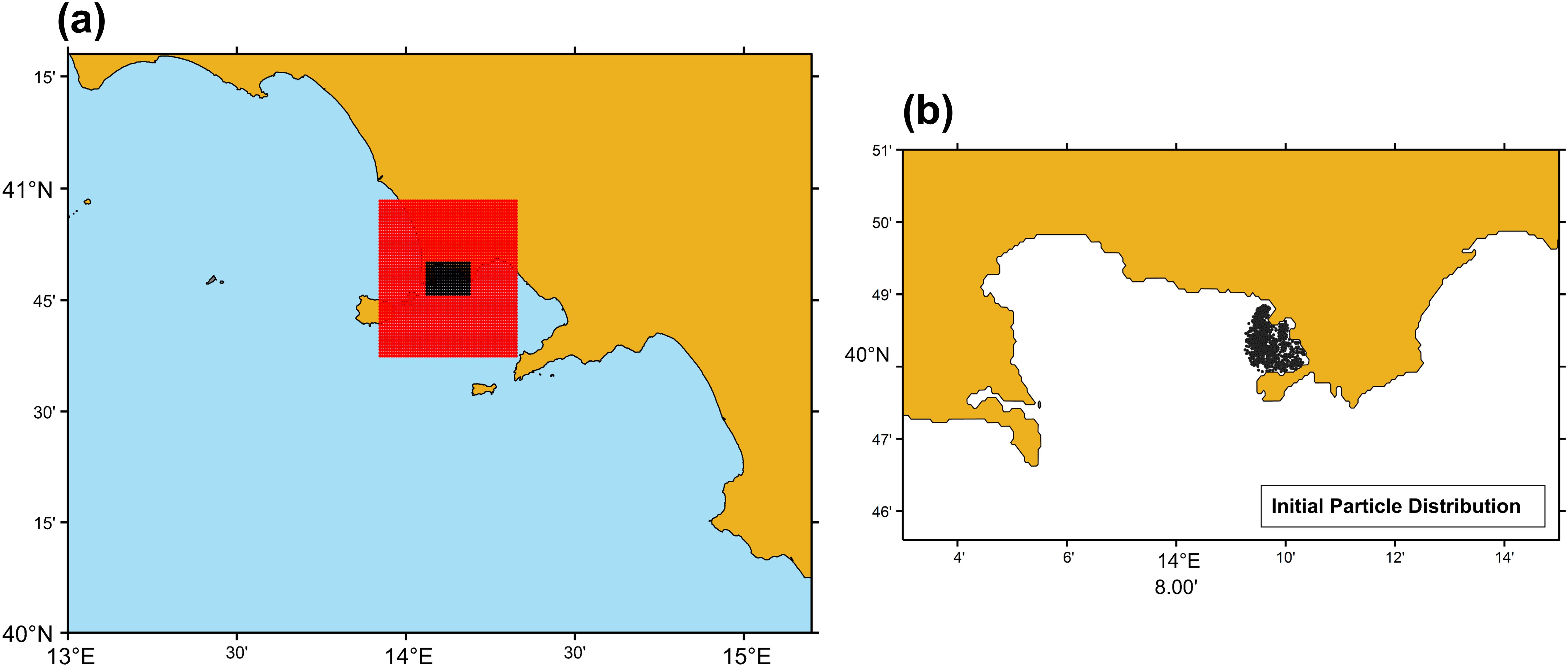
Figure 3. (a) Target area (black box) and the surrounding buffer zone (red box) used for the computation of the blended wind field. (b) Initial particle distribution adopted for Lagrangian transport simulations.

$\begin{array}{ll}W(d)=\frac{1}{2}(1+cos(\pi *\frac{d}{R}\left)\right)\text{\hspace{0.33em}\hspace{0.33em}\hspace{0.33em}\hspace{0.33em}\hspace{0.33em}for d}<\text{R}& (1)\end{array}$

where d is the distance from the boundary of the black box, and R is the relaxation distance defining the width of the transition. This function ensures that the observed wind has full weight at the boundary of the target area (W = 1 at d = 0) and smoothly fades to zero (W = 0 at d = R), avoiding artificial discontinuities.

The final wind components (Uadj, Vadj) were then computed according to the following Equations 2 and 3:

$\begin{array}{ll}Uadj=W*Uobs+(1-W)*Ucrom& (2)\end{array}$

$\begin{array}{ll}Vadj=W*Vobs+(1-W)*Vcrom& (3)\end{array}$

2.6 Lagrangian transport simulations

To investigate the transport pathways of contaminants in the coastal environment, forward Lagrangian transport simulations were conducted using the General NOAA Operational Modeling Environment (GNOME) as the modeling tool (Beegle-Krause, 1999; 2001; Zelenke et al., 2012). The simulations were driven by the Eulerian surface current fields produced by the CROM and forced with the blended wind field. GNOME applies a mixed Eulerian-Lagrangian approach to simulate the particles’ advection (Lagrangian Elements, LEs) driven by time-varying surface currents and/or wind forcing, using a forward Euler integration scheme (equivalent to a first-order Runge-Kutta method). Particles are modeled as passive tracers, and transport is constrained to a single surface layer, neglecting vertical motions and shear. In GNOME, the displacement (Δx, Δy, Δz) at time t of a generic passive tracer (identified by its spatial coordinates) is calculated using Equation 4 (Zelenke et al., 2012):

$\begin{array}{ll}\mathrm{\Delta }x=\frac{\frac{u}{111,120.00024}*\Delta t}{\cos (y)},\mathrm{\Delta }y=\frac{v}{111,120.00024}*\mathrm{\Delta }t,\text{\hspace{0.33em}and\hspace{0.33em}}\mathrm{\Delta }z=0& (4)\end{array}$

where Δt = t − t₁ is the time elapsed between time steps i (set to 15 minutes), y is the latitude in radians, and 111120.00024 is the distance in meters per degree of latitude (assuming 1 arcminute equals 1 nautical mile everywhere). (Δx, Δy) are the 2D longitudinal and latitudinal displacements at the surface layer z, while (u, v) are the zonal and meridional components of the surface current field provided by CROM.

Diffusive processes were also included in the transport equations, using GNOME’s random walk algorithm. The horizontal diffusion is represented as (Zelenke et al., 2012) using Equation 5:

$\begin{array}{ll}\frac{\partial C}{\partial t}=D_x*\frac{{\partial }^{2}C}{\partial x^2}+D_y*\frac{{\partial }^{2}C}{\partial y^2}& (5)\end{array}$

Where C is the concentration of the material and $D_x$, $D_y$ are the horizontal diffusivity coefficients.

Considering the diffusive processes, the calculation of the zonal (Δx) and meridional displacement (Δy) of the i-th particle is computed according to the following Equation 6:

$\begin{array}{ll}\begin{array}{c}\text{Δ}x=\frac{dx*\frac{\sqrt{6*\frac{D}{10,000}*\text{Δ}t}}{111,120.00024}}{\cos (y)},\text{ Δ}y\\ =dy*\frac{\sqrt{6*\frac{D}{10,000}*\Delta t}}{111,120.00024}\end{array}& (6)\end{array}$

GNOME then calculates the horizontal displacements using the diffusion coefficient D, and at each time step, it randomly selects dx and dy from a uniform distribution ranging between -1 and 1.

Following Uttieri et al. (2011), the horizontal diffusion was set equal to 10⁴ cm²/s, a typical value for coastal areas (Okubo, 1971). Regarding particle beaching, GNOME automatically checks whether the new particle position is located on land or in water. The beaching algorithm traces the entire line on the bitmap between the old and new points to ensure that the particle does not skip over land and instead stops it at the first land cell encountered.

Based on the analysis of observed meteo-marine conditions for each event, we hypothesize that PAH-bearing sediments are resuspended during high-energy wave events and subsequently transported by surface currents from Bagnoli to the Lucrino mussels farm (red point in Figure 1).

To simulate this process, 4000 virtual particles were randomly released within the Bagnoli coastal zone (see the black dots in Figure 3b). Releases were triggered one day after each peak wave event to account for a time lag between sediment resuspension and the onset of transport. Supplementary Table 1, provided in the Supplementary Material, summarizes each simulation experiment’s timing and duration (in hours).

To account for uncertainties in the simulated current field, a 30% error estimate was applied to both the along-current and cross-current components. This approach enables the calculation of both a best-guess trajectory (based on the unperturbed current field) and a corresponding minimum regret trajectory that captures the range of plausible transport pathways under uncertain conditions. Simulating the minimum regret solution helps assess transport outcomes that are less probable but potentially more harmful than the best-guess scenario.

2.7 Satellite data

Understanding surface circulation patterns in the GoP and in the GoN is crucial for analyzing transport dynamics in the study area. To complement the “MEDA A” and CROM surface circulation datasets for each pollution event in 2016, we incorporated satellite-derived chlorophyll-a (CHL) concentration data covering the study area. While CHL data do not provide a direct measurement of surface currents, they offer valuable qualitative insights into hydrodynamic patterns, as chlorophyll distribution is influenced by water mass movements, mixing processes, and frontal dynamics (Mattei and Scardi, 2022; Dohan, 2017; Forget and André, 2007). This makes it a useful indicator of surface circulation features.

Satellite CHL observations have been widely used to study oceanographic processes and assess surface circulation patterns. In this study, CHL satellite data provided an additional observational component to evaluate the consistency between modeled circulation fields and features visible in ocean color imagery.

For this purpose, we used the Mediterranean Sea, Bio-Geo-Chemical, L4, monthly means, daily gap-free and climatology Satellite Observations product (Product ID: OCEANCOLOUR_MED_BGC_L4_MY_009_144) from the Copernicus Marine Environment Monitoring Service (CMEMS, https://marine.copernicus.eu/). This dataset provides daily, gap-free CHL concentration data at a 1 km spatial resolution and a Level 4 processing level, ensuring high-quality, temporally consistent estimates for the Mediterranean Sea (Volpe et al., 2018, 2019). The dataset was accessed through CMEMS and is available at https://doi.org/10.48670/moi-00300.

This choice was driven by the limited availability of higher-resolution satellite data (Levels 1 and 2), which are significantly affected by cloud cover, particularly during the winter months. While Kd490 (the diffuse attenuation coefficient at 490 nm) could have been a valuable proxy for sediment transport in this study, its spatial resolution and temporal coverage during the period of interest were insufficient for our analysis. Consequently, we opted to rely exclusively on CHL data for comparison with observed sea current patterns.

Satellite data were processed, analyzed, and visualized using MATLAB and SeaDAS, a specialized image analysis package developed by NASA for processing, displaying, analyzing, and ensuring the quality control of ocean color data.

Supplementary Table 2, in the Supplementary Material, summarizes all the data used in this study, including their type and availability.

3 Results

As previously described, the GoP is a relatively small bay located in the northwestern part of the GoN. Among other contaminants, the levels of PAHs in mussels from the Lucrino farming site (Figure 1) show a marked seasonality (Figure 4), potentially attributed to seasonal variability in wind and sea surface current patterns (Esposito et al., 2017). Therefore, PAH concentrations may be influenced by hydrodynamics within the GoN (Perugini et al., 2007a), as well as by seasonal variations in biotic and abiotic factors governing PAH metabolic processes and bioaccumulation (Perugini et al., 2007b). Numerous studies in other coastal areas in the Mediterranean Sea (Balcıoğlu, 2021; Tepe et al., 2022), as well as at a global scale (Reddy et al., 2005; Zhang and Tao, 2008; Koudryashova et al., 2019; Miura et al., 2019; Recabarren-Villalón et al., 2021) have shown seasonal variability in PAH contamination. The monitoring results from 2014 to 2022 (Figure 5) confirmed the trend already verified in past years, with high PAH levels in the winter period and close to zero in the spring and summer seasons. In particular, in 2016, over a total of 15 samples, only 4 were found to have levels exceeding the legal limits established by the legislation. High contamination events were observed only during late autumn and early winter mussel sampling, specifically on the following dates: 25th of January, 17th of February, 22nd of November, and 14th of December. Figure 5 shows the variability of BaP and the sum of the four PAHs collected in mussel tissues throughout 2016.

Figure 4

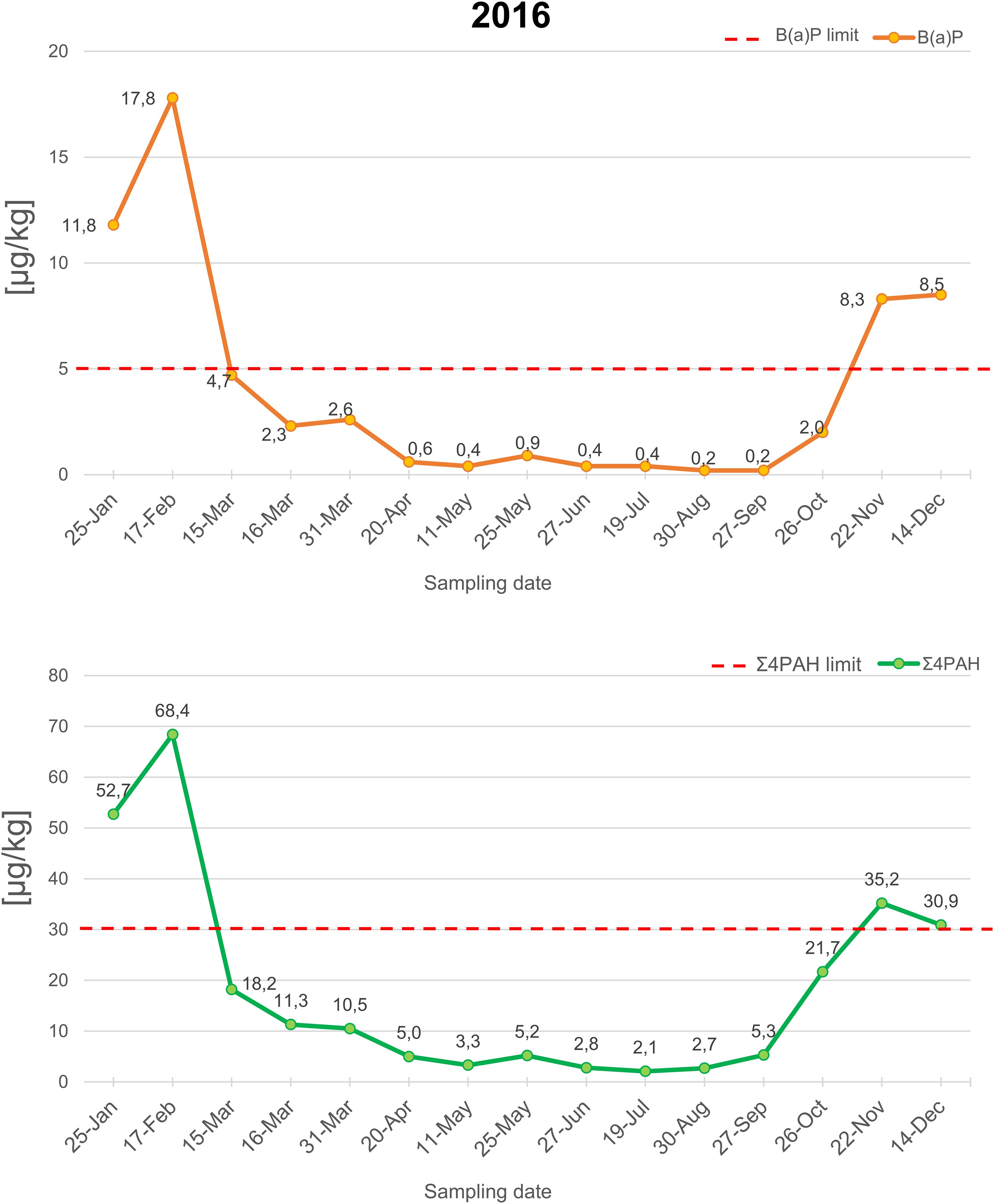
Figure 4. BaP concentration levels (upper panel) and sum of 4PAH concentration (lower panel) in Mytilus galloprovincialis, tissues from Lucrino farm in 2016. The red dotted line indicate the PAHs legal limit. Dates refer to each PAH concentration analysis performed on samples mussels.

Figure 5

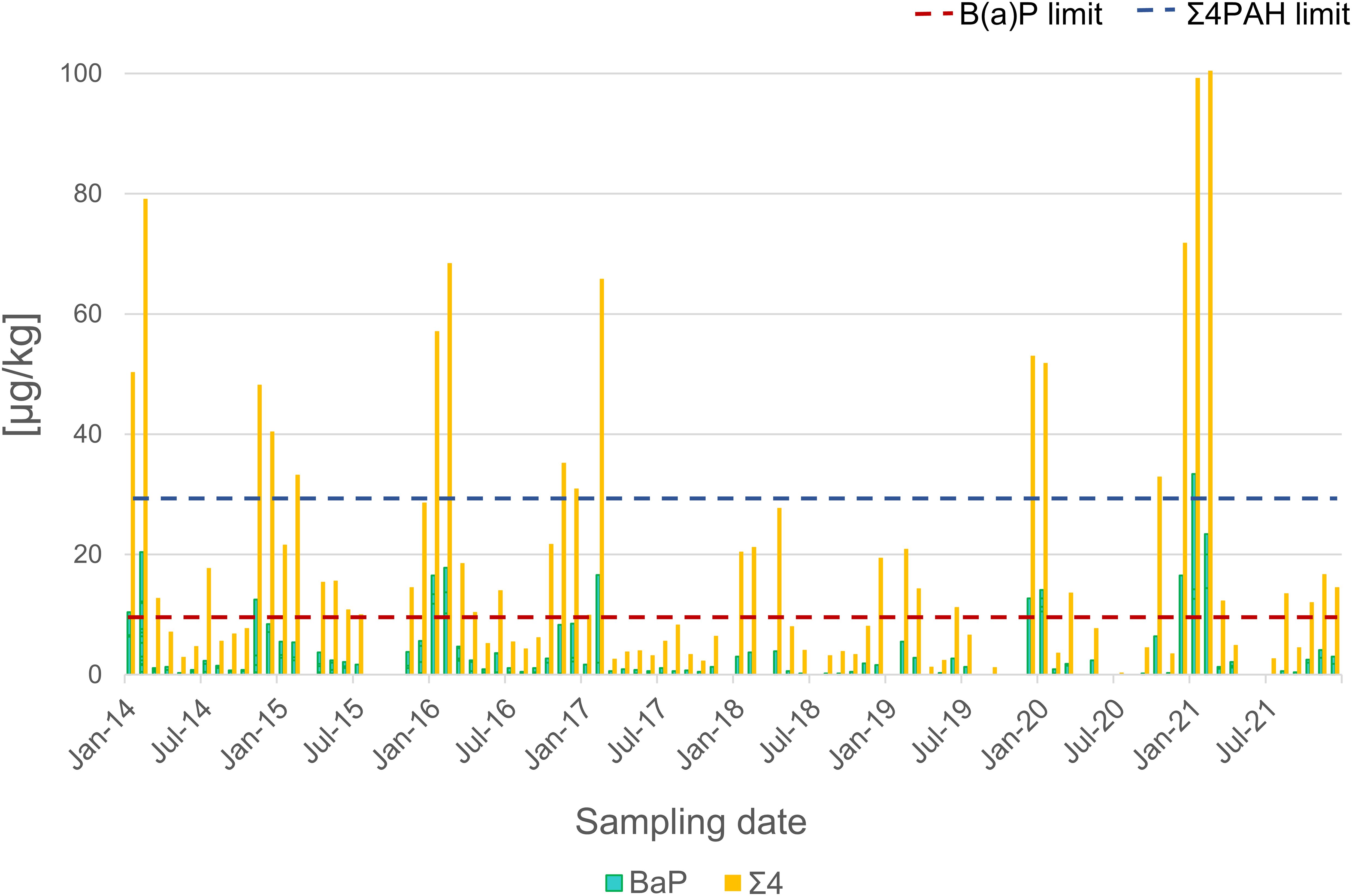
Figure 5. BaP concentration levels and sum of 4PAH concentration in Mytilus galloprovincialis, tissues from Lucrino farm between 2014 and 2022. The dotted lines indicate the PAHs legal limit.

This area is still characterized by a notable lack of in situ, depth-resolved oceanographic data, limiting the understanding of local circulation patterns.

The data collected by the ‘MEDA A’ CTD probe were used to analyze the physical characteristics of the ocean. The temperature-salinity diagram of Figure 6 shows that their values during the contamination episodes did not differ significantly from those of the month. Seasonal patterns emerged from our analysis, with colder and saltier water masses prevalent in winter (minimum temperature: 14.24°C, maximum salinity: 38.19 PSU), and less cold, less salty water masses during summer months (maximum temperature: 27.82°C, minimum salinity: 34.10 PSU). The least salty mass of water (green in the T-S diagram) corresponds to the early May period. This freshwater is justified by the relative increase in rainfall, with peak amounts reaching 27.2 mm recorded by the Pozzuoli weather station. The sea current data collected by the ‘MEDA A’ ADCP were used to examine the physical dynamics of the water column. Hovmöller diagrams illustrate the daily averages of zonal (u) and meridional (v) components of the sea currents, spanning depths from 1.4 m to 18.5 m. The Hovmöller diagram (Figure 7a) for the entire year provides a comprehensive overview of the oceanographic conditions preceding each sampling event. Notably, before high PAH contamination events in late autumn and early 2016, the entire water column exhibited a negative zonal component (u) and a positive meridional component (v), indicating westward transport. This pattern suggests a potential accumulation of pollutants in the western area of GoP, where mussel farms are located. During the summer of 2016, the same north-westward pattern was only found in the surface layers. The absence of the same combination of conditions throughout the water column suggests that pollutant transport mechanisms differ significantly between winter and summer. During the warmer months, the sea surface circulation suggests that pollutants may not be effectively transported to deeper layers or across broader areas. In winter, however, prolonged and intense wind activity leads to the intensification of wind-induced currents, enhancing the transport of pollutants along the coast and potentially leading to localized contamination. In contrast, during summer, the lower intensity wind-induced currents likely reduce pollutant dispersion, decreasing the risk of contamination beyond legal limits. However, the risk remains, as even under more stable conditions, pollution can still occur, although it is less frequent or intense. The seasonal behavior of sediment transport aligns with the typical development of the mixed layer during different seasons at mid-latitudes (Cianelli et al., 2011).

Figure 6

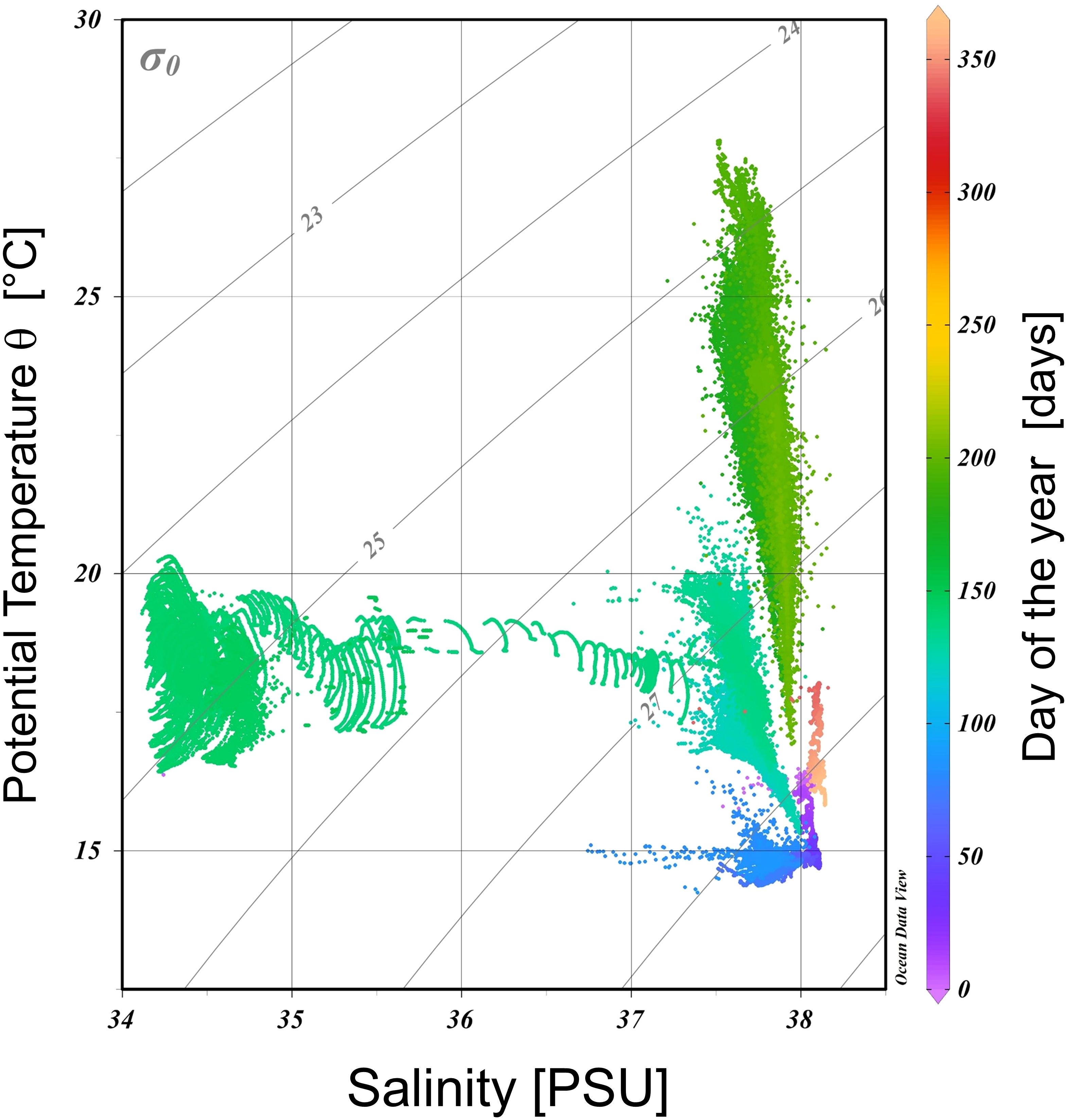
Figure 6. Potential temperature-Salinity (θ-S) diagram for the 2016. The colorbar indicates the days of the year. Data were collected at a depth of 15m from the "MEDA A" CTD probe.

Figure 7

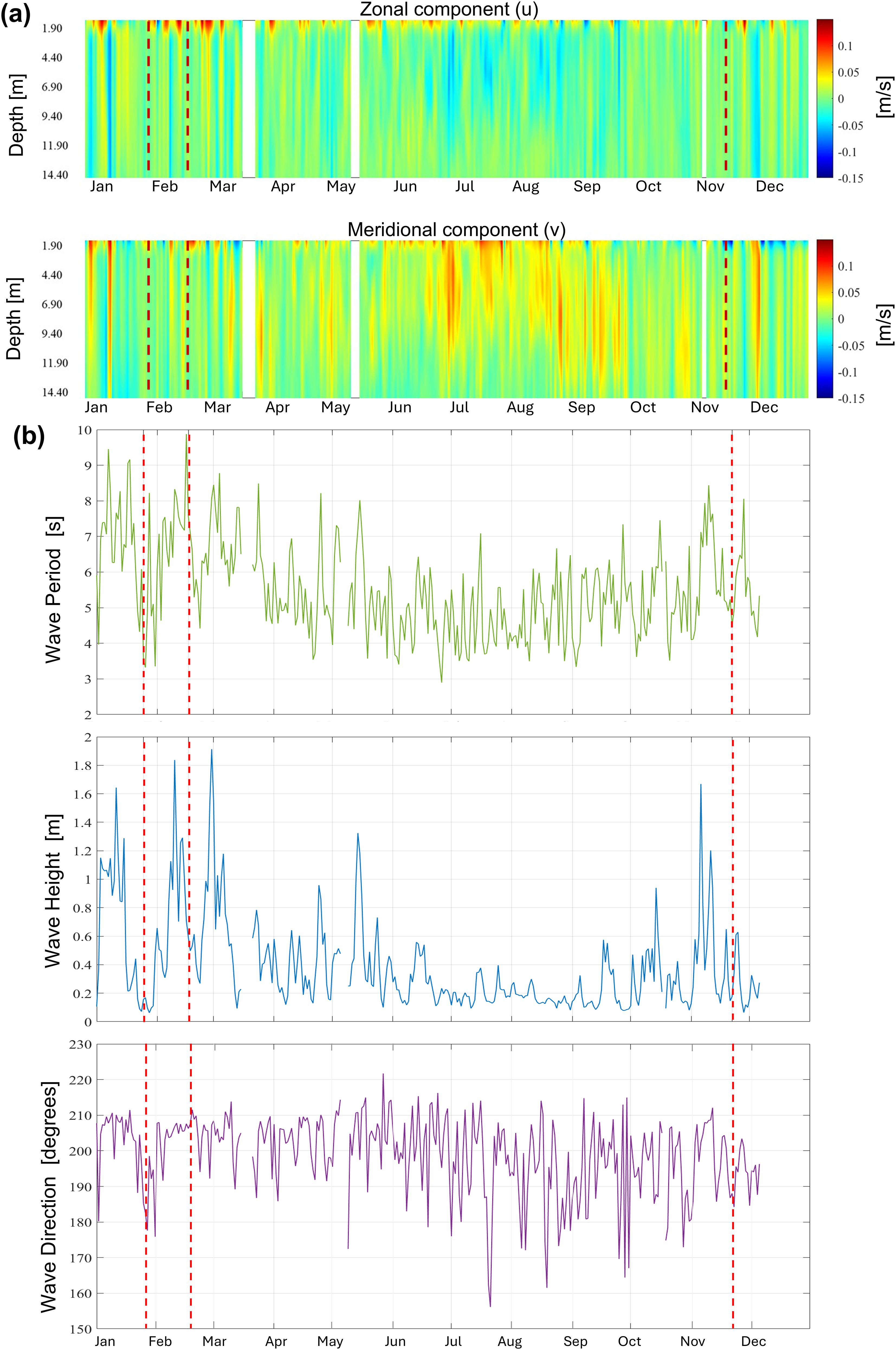
Figure 7. (a) Hovmöller diagram for sea current data. The labels on the x-axis are the dates of mussel sampling and relative PAH analyses. (b) Wave period, wave height, and wave direction recorded by "MEDA A" ADCP in 2016. The dotted red lines indicate events and with higher contamination.

In addition to current velocity, the ADCP also recorded wave height, direction, and period. The wave data (Figure 7b) reveal that, prior to pollution events, wave heights were generally higher, with peak wave periods (T_p) longer than 8 s and a predominant direction from the south. In particular, significant wave heights (H_s) exceeding 1.2 m consistently preceded the most significant PAH contamination episodes. These wave conditions indicate enhanced hydrodynamic forcing capable of mobilizing surface sediments. To quantify the potential for sediment resuspension, wave-induced bottom shear stress (τ_p) was estimated using the Soulsby (1997) and Nielsen (1992) formulation, based on ADCP-measured wave parameters (H_s = 1.2 m, T = 8 s) and a representative site depth of 19 m. Assuming a wave friction factor appropriate for sandy seabed (f^w = 0.04), the calculated τ_p (~2.9 Pa) clearly exceeds the critical shear stress for fine sand resuspension (τc ≈ 0.05–0.1 Pa). This quantitative evidence confirms that the wave energy thresholds required to trigger sediment resuspension were surpassed, supporting the role of wave dynamics in enhancing PAH release into the water column and increasing their bioavailability. These findings align with the unified sediment transport framework proposed by Van Rijn et al. (2007), which emphasizes the combined effects of currents and waves in controlling sediment mobilization and transport dynamics. The predominance of fine sand in the study area, as documented by Arienzo et al. (2017), justifies the use of these τc values and supports the application of this framework to interpret sediment resuspension and contaminant dynamics at the Lucrino site.

In this section, we describe the atmospheric pattern and the ocean properties before and during each high PAH concentration event, aiming at identifying any recurring pattern in marine-weather conditions that might contribute to the presence of high PAH levels in the area. To this goal, stick diagrams of the observed wind and sea currents have been obtained, using meteorological data from the Bacoli station and oceanographic data collected from the “MEDA A” in Bagnoli. Furthermore, to gain a broader large-scale view of marine conditions during the investigation periods, ocean model data and satellite observations have been analyzed. The sea surface current fields simulated by CROM in the GoN and GoP were analyzed since one week before the mussel sampling dates that recorded a higher PAH concentration (hereafter referred to as the pollution event). Analyses for each event are presented and discussed below, providing insights into the complex interplay between atmospheric dynamics, oceanic currents, and pollution events in the region.

25^th January pollution event

The PAH levels measured on 25 January 2016 were 11.8 μg/kg for BaP and 52.7 μg/kg for the sum of the four PAHs. Wind data of the entire month indicate a single episode of strong SSE winds (around January 20), with peak speeds reaching 10.8 m/s, approximately one week prior to the pollution event. This is evident in Figure 8a where, the arrows indicate the direction the wind is pointing at. This convention is applied to similar diagrams (Figures 7–10) for wind and current data. On a larger scale, from January 18th to 22nd, the study region was affected by an atmospheric weak trough, resulting in a northeastern flow associated with minor precipitation events. Specifically, a brief rainfall episode occurred on the 21st, attributed to the passage of an instability line (i.e., a non-frontal band of convective activity). Following this, a gradual rise in atmospheric pressure was observed as a high-pressure system migrated into the Central Mediterranean basin, ensuring stable meteorological conditions until 25th January. During this period, northerly winds still prevailed, except on the day 25th, when winds shifted from the northwest due to the presence of the anticyclonic area.

Figure 8

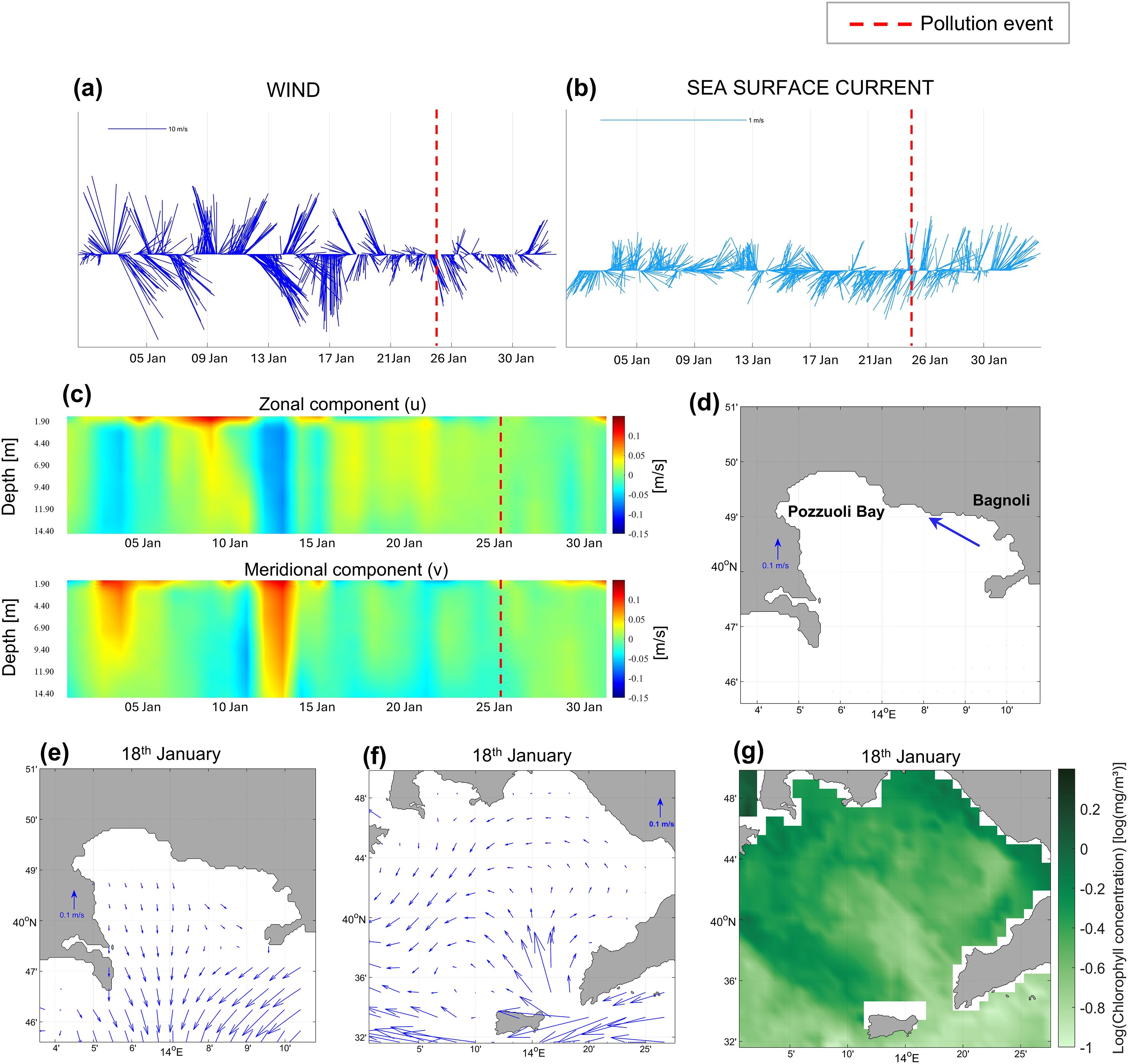
Figure 8. (a) Stickplot diagram for wind data in January 2016; (b) Stickplot diagram for sea surface current data recorded by the ADCP probe in January 2016; (c) Homöller diagram for sea current data in January 2016; (d) Mean current velocity map; (e) Daily map of surface current simulated by CROM one week before the pollution event on 25th January zoomed in GoP. The arrows indicate the direction and intensity of the sea surface currents; (f) Daily map of surface current simulated by CROM one week before the pollution event on 25th January over the GoN; (g) Daily Level 4 CHL maps at 1 km of spatial resolution to describe the conditions of the enquired area about a week before the pollution event on 25th January.

Figure 9

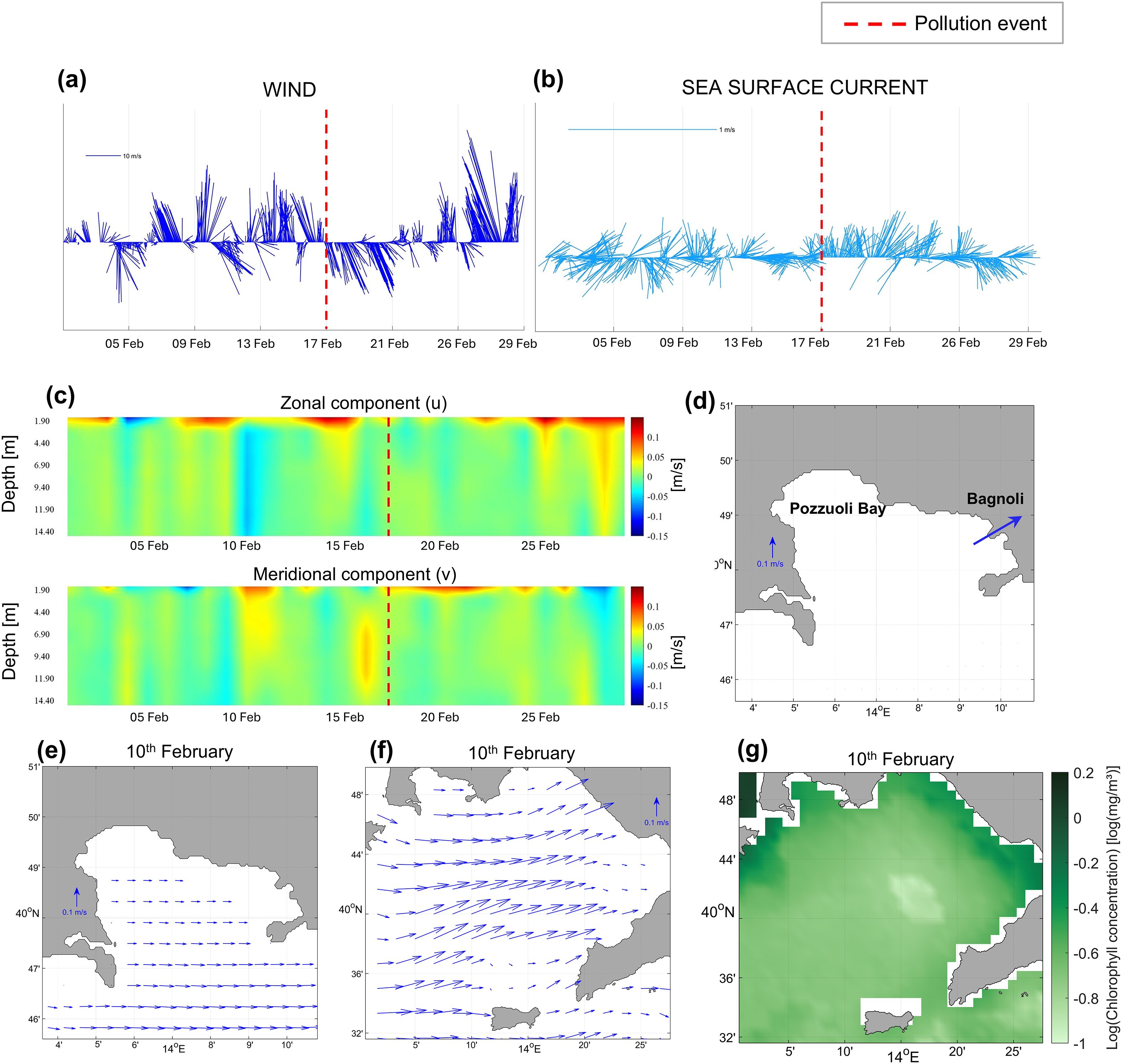
Figure 9. (a) Stickplot diagram for wind data in February 2016; (b) Stickplot diagram for sea surface current data recorded by the ADCP probe in February 2016; (c) Homöller diagram for sea current data in February 2016; (d) Mean current velocity map; (e) Daily map of surface current simulated by CROM one week before the pollution event on 17th February zoomed in GoP. The arrows indicate the direction and intensity of the sea surface currents; (f) Daily map of surface current simulated by CROM one week before the pollution event on 17th February over the GoN; (g) Daily Level 4 CHL maps at 1 km of spatial resolution to describe the conditions of the enquired area about a week before the pollution event on 17th February.

Figure 10

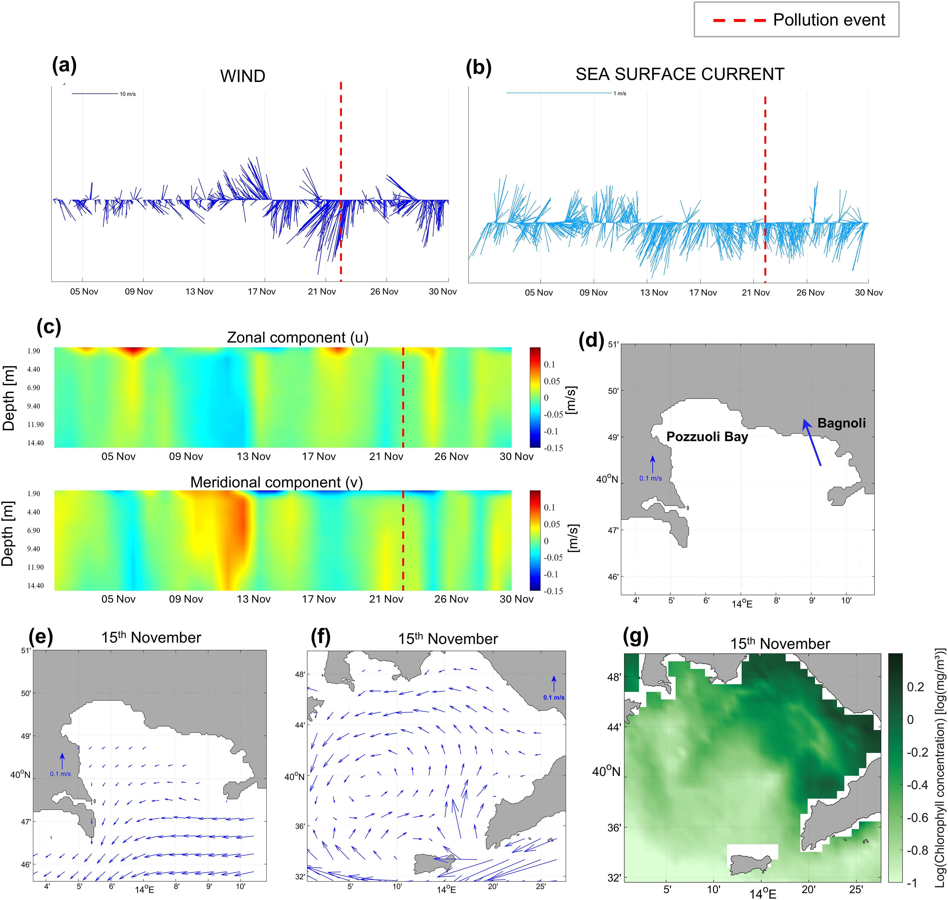
Figure 10. (a) Stickplot diagram for wind data in November 2016; (b) Stickplot diagram for sea surface current data recorded by the ADCP probe in November 2016; (c) Homöller diagram for sea current data in November 2016; (d) Mean current velocity map; (e) Daily map of surface current simulated by CROM one week before the pollution event on 22nd November zoomed in GoP. The arrows indicate the direction and intensity of the sea surface currents; (f) Daily map of surface current simulated by CROM one week before the pollution event on 22nd November over the GoN; (g) Daily Level 4 CHL maps at 1 km of spatial resolution to describe the conditions of the enquired area about a week before the pollution event on 22nd November.

ADCP data (Figure 8b) indicates that sea currents were predominantly directed towards SW-WSW during January 2016, with a temporary change in current direction about ten days before the pollution event. The Hovmöller diagram derived from ADCP data (Figure 8c) provides crucial insights into the currents preceding the pollution event. Approximately ten days before the event, across all the analyzed depths, the zonal component (u) was observed to be negative, while the meridional component (v) was positive, indicating a prevailing movement of sea currents towards the NW. During this timeframe, the zonal component reached its maximum negative value (− 0.089), while the meridional component reached a maximum value of 1.1 cm/s. Figure 8d illustrates the mean current during this period, recorded at 0.06 cm/s.

The analysis of model outputs shows a southwestward current in the central and offshore areas of the GoN (Figures 8e, f) one week prior to the pollution event. Moreover, the satellite CHL maps (Figure 8g) reveal a lower concentration in the Bocca Piccola area of the GoN, which aligns with the circulation pattern described by CROM that shows an entering flow from Bocca Piccola. This confirms that despite the model’s limitations in near coastal coverage, it might still capture significant circulation patterns affecting the distribution of CHL and, potentially, other particles.

17^th February pollution event

The PAH levels measured on 17^th February were 17.8 µg/kg for BaP and 68.4 µg/kg for the sum of the four PAHs. Large-scale atmospheric circulation analysis shows that during the period from 10th to 13th February, the Central Mediterranean area was affected by a western flow, embedded in a wide trough that embraced a large part of Central and Northern Europe. This led to several moderate rainfall episodes in the study area, especially on February 11th and 13th. On the 14th, a notable meridional oscillation of the polar front occurred over the western Mediterranean basin, triggering a southern and mild flow over the Italian Peninsula. Such meridional flow caused additional weak rainfall events on the 14th and 15th February. In the subsequent days, the Rossby wave evolved to the cutoff stage between the Balearic Islands and northern Africa, leading to warm advection over Southern Italy without generating significant precipitation events.

The local wind data analysis (Figure 9a) indicates that strong SSE-S winds were observed one week prior to the pollution event, with peaks reaching a maximum of 16.9 m/s.

In this scenario, the sea surface current pattern at the “MEDA A” site (Figure 9b) exhibited more variability compared to January. However, the current field is directed towards NE in both the surface and immediate subsurface layers. Below approximately 4 meters, a predominant direction towards NW was observed. (Figure 9c). During this period, the zonal component of the current reached a maximum value of 0.6 cm/s, while the meridional component reached a maximum value of 0.4 cm/s. The resulting mean current intensity was reported as 0.6 cm/s (Figure 9d).

The sea surface circulation simulated by CROM one week before the pollution event (Figures 9e, f) shows a flow mainly directed towards the eastern area of the GoP.

The CHL concentration map (Figure 9g) shows a minimum concentration near the Gulf of Castellammare di Stabia that could be associated with the presence of a gyre that is consistent with the Eulerian current field simulated by CROM.

22^nd November pollution event

The PAH levels measured on 22^nd November were 8.3 µg/kg for BaP and 35.2 µg/kg for the sum of the four PAHs. In situ wind data (Figure 10a) showed a variable regime with relatively weak winds throughout the month, except for the week preceding the pollution event during which winds peaked at a maximum of 11.6 m/s, blowing from the SE-SSE.

Initially, the meteorological conditions were modulated by a high-pressure area until the 17th. Subsequently, a wide trough formed over Western Europe, affecting the western side of the Mediterranean region between the 20th and the 22nd of November. This meteorological configuration led to a warm southeastern flow over the Tyrrhenian Sea, determining a rise in air temperature. As for the rainfall, from the 15th to the 22nd of November, no precipitation events occurred in the investigated area. Regarding sea surface currents, variable patterns were observed during the first two weeks of November, as shown by the stickplot diagram in Figure 10b. Then, after the 13^th of November, intense currents directed towards SSW-SW persisted for a continuous two-week period. Around ten days before the pollution event, sea currents were towards the NW, as illustrated by the Hovmöller diagram in Figure 10c. During this period, the zonal component of the current reached a maximum value of 0.2 m/s, while the meridional one reached a maximum value of 0.2 m/s, resulting in a mean current of 0.06 cm/s (Figure 10d).

The sea surface circulation simulated by CROM one week before the pollution event showed a southwestward current in the central and offshore areas of the GoN (Figure 10e, f). Additionally, the satellite CHL maps (Figure 10g) revealed a lower concentration in the Bocca Piccola area of the GoN and a higher concentration near the coast, which aligns with the circulation pattern described by CROM that showed a flow entering from Bocca Piccola. This suggests that, despite the model’s limitations in coastal areas, it still provides valuable insights into the circulation patterns that influence the distribution of CHL and, potentially, other particles.

14^th December pollution event

The PAH levels measured on 14^th December were 8.5 µg/kg for BaP and 30.9 µg/kg for the sum of the four PAHs. From the 8th to the 10th of December, the atmospheric conditions in the study area were modulated by a high-pressure system, which determined stable weather, light winds and an absence of precipitation events. On the 11^th of December, a wide trough affected Eastern Europe and the Balkan Peninsula, weakening the high-pressure system. Consequently, a weak low-pressure area formed over the Ligurian Sea, driving a moist western flow over the investigated area, leading to light rainfall around the 11th and 12th of December. In the following days, the synoptic configuration was characterized by an anticyclonic area over the Central Mediterranean region and Central Europe, along with a trough elongated from Eastern Europe to the Eastern Mediterranean. Stable weather conditions prevailed over the study area, associated with moderate northeastern winds. Prior to the pollution event, strong SE-SSE winds were locally observed, with peaks reaching 16.1 m/s, as shown in the stickplot diagram in Figure 11a. Unfortunately, current data were only collected until December 6^th by “MEDA A”, limiting the discussion of the current pattern for the entire month. Nevertheless, the observation period included the week before the pollution event on December 14th. Analysis of sea surface currents (Figure 11b) indicated that they were predominantly directed towards the SSW-SW direction. The Hovmöller diagram (Figure 11c) showed that the period preceding the pollution event was characterized by a column of water with a negative zonal component (u) and a positive meridional component (v). During this period, the zonal component reached a maximum value of 9.7 cm/s, while the meridional component reached a maximum value of 9.6 cm/s. The average of the prevailing directions of marine currents is represented in Figure 11d.

Figure 11

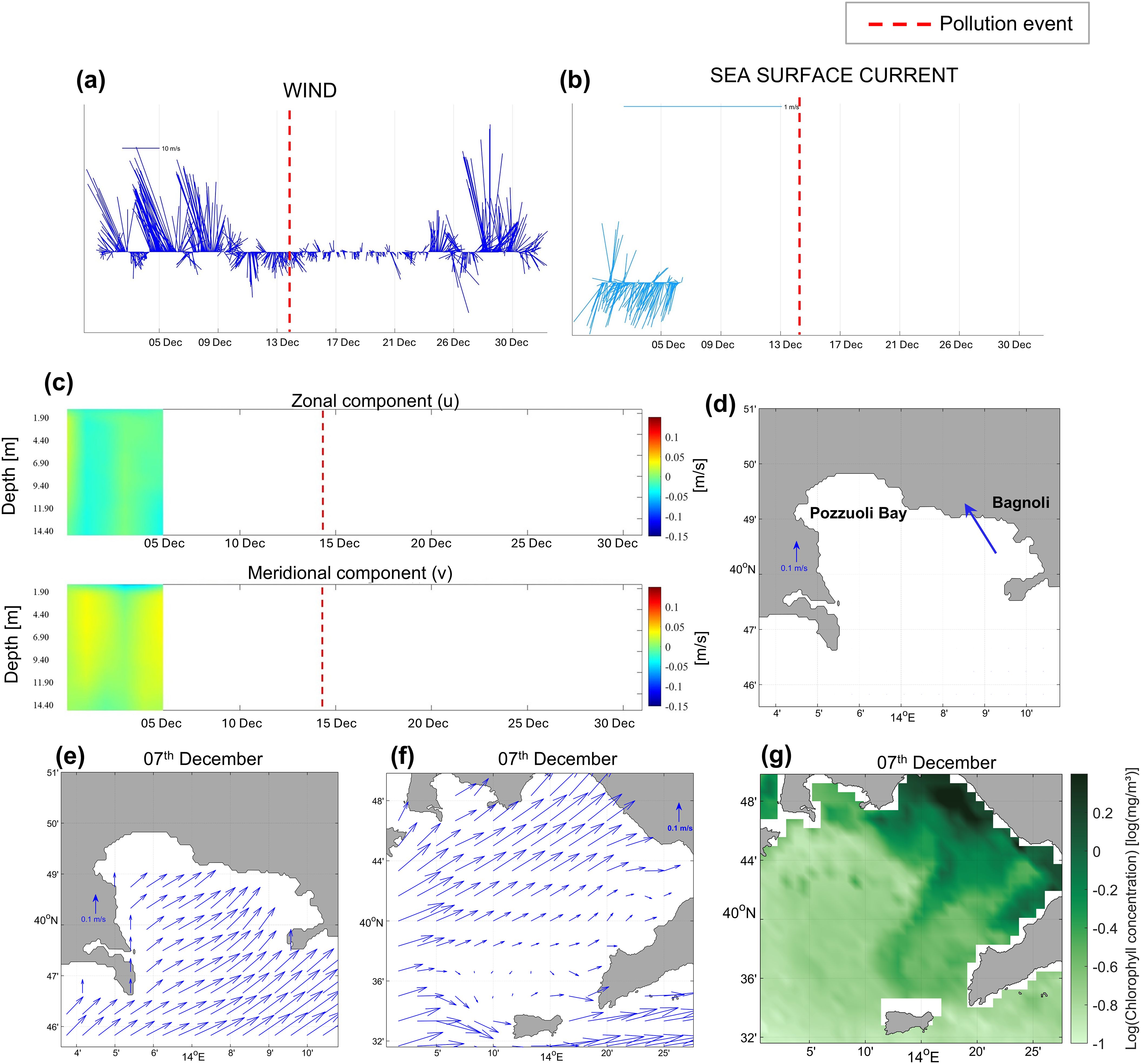
Figure 11. (a) Stickplot diagram for wind data in December 2016; (b) Stickplot diagram for sea surface current data recorded by the ADCP probe in December 2016; (c) Hovmöller diagram for sea current data in December 2016; (d) Mean current velocity map; (e) Daily map of surface current simulated by CROM one week before the pollution event on 14th December zoomed in GoP. The arrows indicate the direction and intensity of the sea surface currents; (f) Daily map of surface current simulated by CROM one week before the pollution event on 14th December over the GoN; (g) Daily Level 4 CHL maps at 1 km of spatial resolution to describe the conditions of the enquired area about a week before the pollution event on 14th December.

The sea surface current simulated by CROM one week before the pollution event (Figures 11e, f) showed a flow mainly directed towards the eastern area of the GoP. This flow aligns with the observed CHL patterns (Figure 11g), indicating a high concentration of CHL in the GoN, where the entering flow is consistent, and a lower CHL concentration in the GoP.

3.1 Simulated transport scenarios

Once the atmospheric forcing acting on the study area before and during the pollution events, along with the corresponding in situ current measurements, have been described, we present here the results of the Lagrangian transport simulations conducted to identify potential sources of PAHs (Polycyclic Aromatic Hydrocarbons) observed in mussels from the Lucrino farm.

This section reports the outcomes of forward Lagrangian simulations designed to test the hypothesis that the Bagnoli site may act as a source of PAHs. For specific details regarding the timing and duration of each simulated scenario, please refer to Supplementary Table 1.

Figure 12 displays the spatial distribution of particle trajectories corresponding to each pollution event. The maps combine particle density plots based on the ‘best guess’ trajectories (shown in grayscale) with the minimum regret solution (pink area in Figure 12), which incorporates uncertainty in surface current simulations. Density maps were generated by dividing the domain into 50 m bins and computing a two-dimensional histogram based on the number of particles traversing each bin throughout the simulation period, thus highlighting the predominant transport pathways and zones of higher particle accumulation. The pink-shaded area represents the uncertainty envelope of the modeled currents; within this area, there is a 90% probability that the particles will be found (Zelenke et al., 2012).

Figure 12

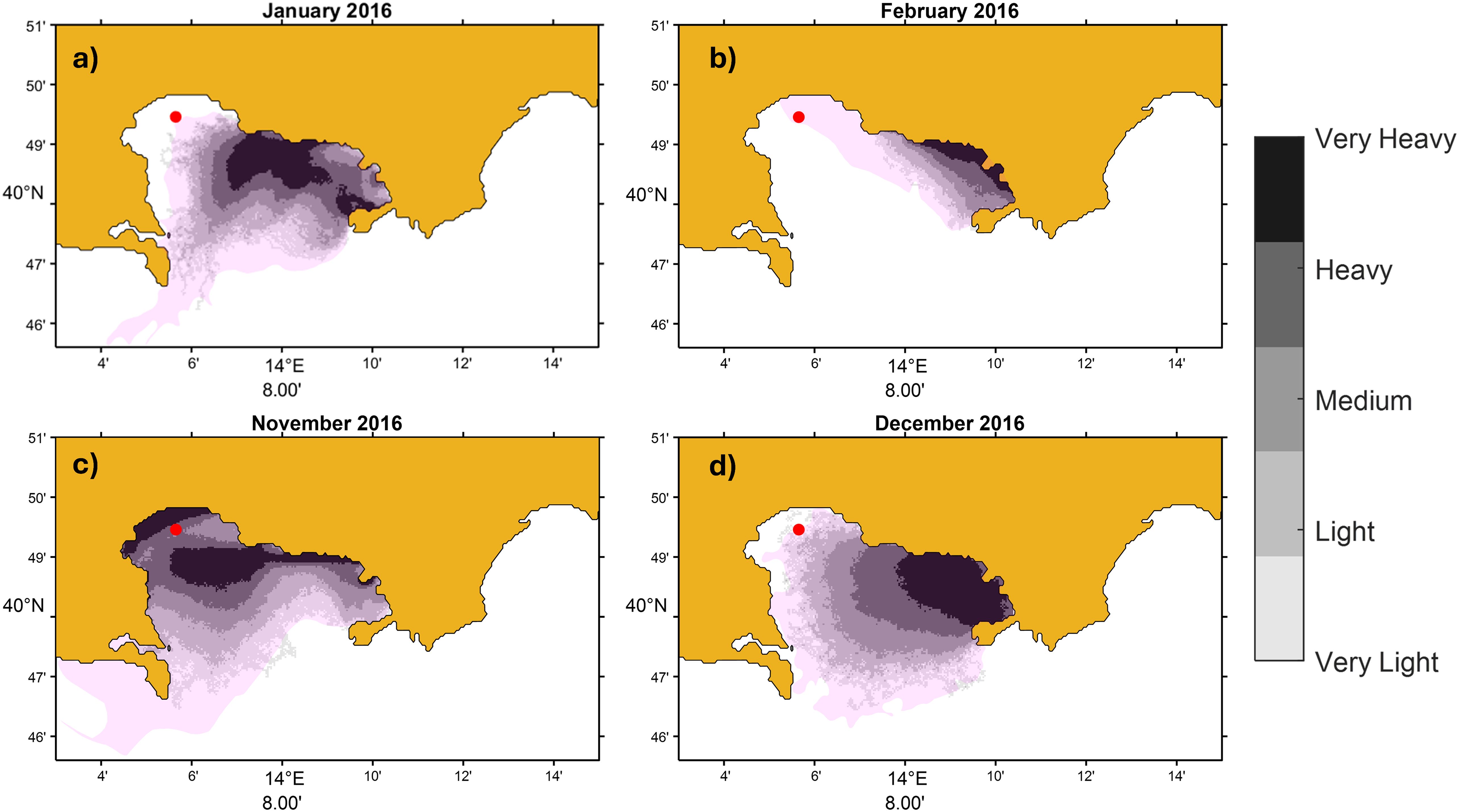
Figure 12. Results of Lagrangian simulations for four high-PAH contamination events: (a) January, (b) February, (c) November, and (d) December 2016. The red dot marks the location of the Lucrino mussel farm. The grayscale shading represents the particle density map obtained considering the 'best guess' solution. The pink-shaded areas indicate the potential spread of particles under uncertain current conditions, obtained by introducing a 30% random perturbation to both the both along- and cross current directions.

Across all four scenarios, forward simulations demonstrate that particles released near Bagnoli can reach the Lucrino mussel farm (indicated by the red dot in Figure 12), although the extent and intensity of this transport vary depending on the specific event. For January 2016 (Figure 12a), the particle plume disperses broadly toward the northwest. Lucrino is located at the plume’s edge, suggesting only limited exposure during this event. For February 2016 (Figure 12b), the best guess trajectories are confined to the northeastern Gulf of Pozzuoli, without directly impacting Lucrino. Nevertheless, when accounting for model uncertainty (pink area), the simulations indicate a potential for particle transport to the mussel farm, highlighting a non-negligible risk. For November 2016 (Figure 12c), a dense and well-defined plume extends westward from Bagnoli, with a significant accumulation of particles around the Lucrino mussel farm.

Finally, for December 2016 (Figure 12d), a broader plume is observed, extending toward Lucrino and reinforcing the potential for contamination transport under suitable conditions.

Overall, the simulation results align with field observations and strongly support the hypothesis that, under specific atmospheric and oceanographic conditions, contaminants resuspended near Bagnoli can be advected toward the Lucrino mussel farm, contributing to the observed PAH concentrations.

4 Discussion

The seasonal behavior of PAH contamination levels in mussels farmed in the GoP reveals periodical events exceeding legal limits during the late autumn and early winter period (Figure 5). Due to the limited availability of in situ along-depth oceanographic data, the analysis was focused on 2016, a year for which both observational and model outputs were more extensively available. This choice was not driven by exceptional environmental conditions, but by data availability. As shown in Figure 5, similar seasonal contamination events were recorded in multiple years, supporting the representativeness of the selected period.

This study addresses a critical gap in the understanding of PAH transport mechanisms in the Gulf of Pozzuoli by integrating in situ observations, satellite data, and numerical models, including forward Lagrangian particle tracking simulations. While previous research documented contamination patterns, the use of Lagrangian simulations to explicitly link pollutant sources—particularly the Bagnoli industrial site—with contamination events at mussel farms represents a novel contribution for this region. This integrated approach allows a more detailed and dynamic understanding of how seasonal meteorological and oceanographic conditions drive pollutant mobilization and accumulation, advancing the state of knowledge in Mediterranean coastal pollution studies.

Our results support the hypothesis that seasonal meteorological and oceanographic variability drives PAH contamination in mussels. We examined meteorological and marine conditions to explore the relationship between wind regimes, sea currents, water mass properties, and contaminant transport mechanisms. This approach aims to improve understanding of the physical processes that concentrate pollutants in the coastal zone and inform targeted mitigation strategies.

Our findings highlight that pollutants resuspended from the heavily polluted coastal area of the Bagnoli site may be transported to the Lucrino mussel farming site, where they could be trapped due to the coastal morphology and inshore currents. The interaction between sea currents and PAH is strongly influenced by the peculiar properties of PAHs. As previously assessed, they can be considered as passively transported substances in the marine environment, primarily influenced by ocean currents, winds, and turbulent motions. These hydrophobic pollutants are characterized by slow environmental degradability with a strong tendency to bind to both organic and inorganic particulate matter suspended in the water and to finally accumulate in the sediments. Accordingly, winds and currents create areas of high concentration in the coastal regions of the GoP, when water column dynamics (i.e. during winter) facilitate the concentration of suspended materials, and thus PAHs. Analysis of current patterns during the four recorded pollution events in 2016 showed predominantly westward flow approximately one week before pollution events. The Hovmöller diagram (Figure 7a) reveals a consistent negative zonal (u) and positive meridional (v) current component during late autumn and early winter, indicating northwestward transport. In contrast, during summer, similar patterns are confined to surface layers, suggesting a seasonal modulation of transport dynamics. These current distributions support the hypothesis that resuspended pollutants from Bagnoli site are advected toward Lucrino, where the coastal morphology and circulation patterns facilitate their accumulation. Low-energy conditions promote deposition of PAHs onto sediments, while energetic events, such as storms or strong currents, can resuspend these particles into the water column (Sun et al., 2018). This cycle of deposition and resuspension influences the bioavailability of contaminants to mussels.

Wave dynamics play a crucial role in sediment mobilization and pollutant release at the study site. ADCP measurements showed consistently elevated wave activity prior to contamination events, with conditions favoring sediment resuspension as indicated by the estimated bottom shear stresses exceeding known critical thresholds for fine sands. This hydrodynamic forcing likely facilitates the remobilization of PAH-bound particles from the seabed, increasing their availability in the water column and uptake by benthic organisms such as mussels.

Moreover, the interplay between wave-induced forces and wind-driven currents appears to be key in shaping the timing and magnitude of contamination episodes. Seasonal variations in current intensity modulate this process, with stronger currents in winter enhancing pollutant dispersal, while calmer summer conditions reduce—but do not eliminate—the risk of contamination.

In support of this hypothesis, the Regional Agency for Environmental Protection of Campania (ARPAC) conducted an environmental survey in 2021 on marine sediments in the GoP (De Maio et al., 2021- sampling activities report). The results of their analyses revealed similar PAH compositions in sediments sampled at Bagnoli and Lucrino. These findings suggest a common contamination source and support the transport pathway.

Forward Lagrangian transport simulations reinforce this conclusion. Under specific wind and current regimes typical of late autumn and early winter, particles released near the Bagnoli site can reach the Lucrino mussel farm. In particular, the November and December 2016 scenarios highlight a significant and well-defined particle plume reaching the Lucrino site, in agreement with the observed high PAH concentrations in mussels. Even in cases where the best-guess trajectories did not directly reach the farm (e.g., February 2016), the inclusion of uncertainty through the minimum regret solution reveals a possible exposure pathway.

The Lagrangian transport simulations presented in this study further strengthen this hypothesis. In all four pollution events analyzed, forward simulations show that particles released near the Bagnoli site can be advected toward the Lucrino mussel farm, although the extent of the transport varies depending on the meteorological conditions.

These results, in conjunction with sediment data and hydrodynamic conditions, confirm that under specific atmospheric and oceanographic conditions, contaminants originating from Bagnoli site are not only mobilized but also effectively transported toward Lucrino site, where they can accumulate.

5 Conclusions

This study demonstrates that seasonal meteorological and oceanographic conditions, particularly wind patterns and sea currents during late autumn and early winter, play a decisive role in the transport and accumulation of PAHs in farmed mussels. The combined analysis of in situ data and Lagrangian transport simulations identifies the eastern part of the Gulf of Pozzuoli, specifically the Bagnoli coastal area, as the dominant source of contamination. The simulations consistently show that, under specific hydrodynamic conditions, contaminants resuspended near Bagnoli can reach the Lucrino mussel farm, aligning with the spatial distribution of contamination observed in mussel tissues and sediments. These findings highlight the need for targeted pollution management strategies that account for seasonal variations in local meteorological and oceanographic conditions. With the identified link between wind-driven circulation and PAH exposure, high-resolution weather and ocean forecasting could serve as a predictive tool for mitigating contamination risk.

By coupling multi-source observational data with advanced modelling and Lagrangian particle tracking, this study fills a significant knowledge gap concerning the physical drivers of PAH contamination in the Gulf of Pozzuoli. The identification of specific meteorological and oceanographic conditions that enable pollutant transport provides a foundation for developing targeted monitoring and management strategies. These findings not only enhance the understanding of pollutant dynamics in this specific coastal system but also offer a transferable framework for similar environments facing anthropogenic contamination challenges.

Based on the findings of this study, several targeted management and monitoring recommendations are proposed to effectively mitigate PAH contamination risks. These include enhancing monitoring throughout the year, with particular attention to late autumn and early winter when contamination levels tend to rise, and integrating meteorological, oceanographic, and chemical data to support early warning systems.

Notably, the demonstrated link between PAH transport and meteo-oceanographic conditions suggests that high-resolution weather and ocean forecasts could serve as powerful tools for preventive management of mussel farming operations. Forecast-based strategies could allow for timely mitigation actions—such as temporary harvesting suspensions, enhanced sampling, or operational adjustments—during high-risk contamination periods. Additional recommendations include targeted sediment remediation or stabilization measures in heavily contaminated coastal areas, such as the Bagnoli site, to reduce the availability of PAHs for resuspension. Expanding monitoring parameters to include key physical variables—such as wave dynamics, current measurements, and turbidity—would enhance our understanding of the mechanisms governing pollutant resuspension and transport. Finally, incorporating long-term environmental data, including precipitation and runoff trends, is essential to improve risk assessments and support sustainable aquaculture management in the GoP and similar coastal systems.

Future studies should implement higher-resolution coastal ocean model, potentially nested with CROM and forced with higher-resolution atmospheric fields. Moreover, incorporating 3D particle tracking tools will enable capturing vertical transport and small-scale circulation effects more accurately, improving the fidelity of pollutant dispersion simulations. Additionally, integrating a water quality model such as WaComM++ (Water quality Community Model Plus Plus) (Giunta et al., 2005; Montella et al., 2016; Galletti et al., 2017; Di Luccio et al., 2017; Montella et al., 2023; Montella et al., 2018; Sánchez-Gallegos et al., 2021), optimized using artificial intelligence algorithms (De Vita et al., 2022a, 2022), could significantly enhance our capacity to simulate and forecast contaminant behavior in complex coastal systems.

Upcoming field efforts will include expanded in situ campaigns involving current measurements, CTD profiling, turbidity monitoring, and water sampling conducted across multiple seasons. Long-term rainfall trends will also be evaluated. Combined with increased chemical monitoring in mussels, these steps aim to deepen our understanding of the coupled physical-biogeochemical mechanisms that drive contamination in coastal environments like the GoP.

The seasonal patterns of PAH contamination observed in the GoP reflect trends documented across the Mediterranean (Balcıoğlu, 2021; Tepe et al., 2022) and globally (Reddy et al., 2005; Zhang and Tao, 2008; Koudryashova et al., 2019; Miura et al., 2019; Recabarren-Villalón et al., 2021). As demonstrated in this study, common meteo-oceanographic forcings are central to these phenomena, highlighting the importance of continuous monitoring and integrated modelling approaches to support environmental risk mitigation and sustainable aquaculture practices in vulnerable coastal systems.

Data availability statement

The raw data supporting the conclusions of this article will be made available by the authors, without undue reservation.

Author contributions

LF: Conceptualization, Data curation, Formal Analysis, Methodology, Software, Supervision, Visualization, Writing – original draft, Writing – review & editing. LG: Data curation, Formal Analysis, Writing – review & editing, Software. ME: Data curation, Writing – review & editing. VC: Data curation, Writing – review & editing. FC: Data curation, Writing – review & editing. PD: Formal Analysis, Writing – review & editing. GA: Conceptualization, Data curation, Methodology, Writing – review & editing. DD: Data curation, Writing – review & editing. EZ: Formal Analysis, Writing – review & editing. GB: Writing – review & editing, Supervision. YC: Conceptualization, Data curation, Formal Analysis, Methodology, Supervision, Writing – original draft, Writing – review & editing.

Funding

The author(s) declare financial support was received for the research and/or publication of this article. This work is part of the project “Un approccio multidisciplinare alla contaminazione da idrocarburi nei mitili allevati nel Golfo di Pozzuoli” funded by the University of Naples Parthenope local research project 2023. This research was partially funded by European Union – NextGenerationEU, National Recovery and Resilience Plan (PNRR), Missione 4 Componente 2 Investimento 1.4 “Potenziamento strutture di ricerca e creazione di campioni nazionali di R&S su alcune Key Enabling Technologies”. Code CN00000023 – Title: Sustainable Mobility Center (Centro Nazionale per la Mobilità Sostenibile) –CNMS. Spoke 3 “Waterways”, Spoke 7 “CCAM, Connected Networks and Smart Infrastructure”. LF’s PhD grant is funded by PNRR, Missione 4 Componente 1 Investimento 3.4 “Potenziamento dell’offerta dei servizi di istruzione: dagli asili nido all’Università” and Investimento 4.1 “Didattica e competenze universitarie avanzate” e “Estensione del numero di dottorati di ricerca e dottorati innovativi per la pubblica amministrazione e il patrimonio culturale”.

Acknowledgments

The authors would like to thank Maurizio della Rotonda (UOD Prevenzione e Sanità Pubblica Veterinaria, Regione Campania) for allowing us to use the data obtained from the chemical monitoring of mussel farms in the Gulf of Pozzuoli. We thank Prof. Raffaele Montella (University Parthenope of Naples) for the important inspiration and suggestions on high-performance environmental computing. We thank Lucio De Maio and Dario Monaco from the “Unità Operativa Mare” of ARPAC (Agenzia Regionale per la Protezione Ambientale della Campania) for providing us with the data related to the environmental surveys in the Gulf of Pozzuoli.

Conflict of interest

The authors declare that the research was conducted in the absence of any commercial or financial relationships that could be construed as a potential conflict of interest.

The reviewer MT declared a past co-authorship with the author ME to the handling editor.

Generative AI statement

The author(s) declare that no Generative AI was used in the creation of this manuscript.

Any alternative text (alt text) provided alongside figures in this article has been generated by Frontiers with the support of artificial intelligence and reasonable efforts have been made to ensure accuracy, including review by the authors wherever possible. If you identify any issues, please contact us.

Publisher’s note

All claims expressed in this article are solely those of the authors and do not necessarily represent those of their affiliated organizations, or those of the publisher, the editors and the reviewers. Any product that may be evaluated in this article, or claim that may be made by its manufacturer, is not guaranteed or endorsed by the publisher.

Supplementary material

The Supplementary Material for this article can be found online at: https://www.frontiersin.org/articles/10.3389/fmars.2025.1565042/full#supplementary-material

References

Abdel-Shafy H. I. and Mansour M. S. M. (2016). A review on polycyclic aromatic hydrocarbons: source, environmental impact, effect on human health and remediation. Egypt. J. Pet. 25, 107–123. doi: 10.1016/j.ejpe.2015.03.011

Crossref Full Text | Google Scholar

Akinsanya B., Adebusoye S. A., Alinson T., and Ukwa U. D. (2018). Bioaccumulation of polycyclic aromatic hydrocarbons, histopathological alterations and parasito-fauna in bentho-pelagic host from Snake Island, Lagos, Nigeria. JOBAZ 79, 40. doi: 10.1186/s41936-018-0046-2

Crossref Full Text | Google Scholar

Albanese S., De Vivo B., Lima A., Cicchella D., Civitillo D., and Cosenza A. (2010). Geochemical baselines and risk assessment of the Bagnoli brownfield site coastal sea sediments (Naples, Italy). J. Geochemical Explor. 105, 19–33. doi: 10.1016/j.gexplo.2010.01.007

Crossref Full Text | Google Scholar

Arienzo M., Donadio C., Mangoni O., Bolinesi F., Stanislao C., Trifuoggi M., et al. (2017). Characterization and source apportionment of polycyclic aromatic hydrocarbons (pahs) in the sediments of gulf of Pozzuoli (Campania, Italy). Mar. pollut. Bull. 124, 480–487. doi: 10.1016/j.marpolbul.2017.07.006

PubMed Abstract | Crossref Full Text | Google Scholar

Arienzo M., Ferrara L., Toscanesi M., Giarra A., Donadio C., and Trifuoggi M. (2020). Sediment contamination by heavy metals and ecological risk assessment: The case of Gulf of Pozzuoli, Naples, Italy. Mar. pollut. Bull. 155, 111149. doi: 10.1016/j.marpolbul.2020.111149

PubMed Abstract | Crossref Full Text | Google Scholar

Armiento G., Caprioli R., Cerbone A., Chiavarini S., Crovato C., de Cassan M., et al. (2020). Current status of coastal sediments contamination in the former industrial area of Bagnoli-Coroglio (Naples, Italy). Chem. Ecol. 36, 579–597. doi: 10.1080/02757540.2020.1747448

Crossref Full Text | Google Scholar

Balcıoğlu E. B. (2021). Sediment contamination by PAHs in Northern Aegean Sea, Gökçeada: Seasonal variations, source determination, and ecological risks. Environ. Forensics 22, 10–15. doi: 10.1080/15275922.2020.1834021

Crossref Full Text | Google Scholar

Baumard P., Budzinski H., and Garrigues P. (1997). Analytical procedure for the analysis of PAHs in biological tissues by gas chromatography coupled to mass spectrometry: application to mussels. Fresenius’ J. Anal. Chem. 359, 502–509. doi: 10.1007/s002160050621

Crossref Full Text | Google Scholar

Beegle-Krause C. J. (1999). “GNOME: NOAA’s next-generation spill trajectory model,” in OCEANS ‘99 MTS/IEEE riding the crest into the 21st century, vol 3 (IEEE/Marine Technology Society, Seattle), 1262–1266. doi: 10.1109/OCEANS.1999.800172

Crossref Full Text | Google Scholar

Beegle-Krause C. J. (2001). “General NOAA Oil Modeling Environment (GNOME): a new spill trajectory model,” in IOSC 2001 proceedings (Mira Digital Publishing, Inc., Tampa, FL), 865–871. doi: 10.7901/2169-3358-2001-2-865

Crossref Full Text | Google Scholar

Bergamin I., Romano E., Gabellini M., Ausili A., and Carboni M. G. (2003). Chemical-physical and ecological characterisation in the environmental project of a polluted coastal area: the Bagnoli case study. Mediterr. Mar. Sci. 4, 5–20. doi: 10.12681/mms.225

Crossref Full Text | Google Scholar

Binelli A. and Provini A. (2003). POPs in edible clams from different Italian and European markets and possible human health risk. Mar. pollut. Bull. 46, 879–886. doi: 10.1016/S0025-326X(03)00043-2

PubMed Abstract | Crossref Full Text | Google Scholar

Bjørseth A. and Ramdahl T. (1985). Handbook of polycyclic aromatic hydrocarbons, volume 2, emission sources and recent progress in analytical chemistry. New York, NY: Marcel Dekker.

Google Scholar

Blumberg A. F. and Mellor G. L. (1987). A description of a three-dimensional coastal ocean circulation model. Three-dimensional Coast. ocean Models 4, 1–16. doi: 10.1029/CO004p0001

Crossref Full Text | Google Scholar

Bonamano S., Piazzolla D., Scanu S., Piermattei V., and Marcelli M. (2021). Trace-metal distribution and ecological risk assessment in sediments of a sheltered coastal area (Gulf of Gaeta, central-eastern Tyrrhenian Sea, Italy) in relation to hydrodynamic conditions. Mediterr. Mar. Sci. 22, 372–384. doi: 10.12681/mms.24996

Crossref Full Text | Google Scholar

Buonocore B., Cianelli D., Falco P., Guida R., Uttieri M., Zambardino G., et al. (2010). Hydrocarbon dispersal in the Gulf of Naples: a parametric study. Rapp Comm Int. Mer Médit 39, 72.

Google Scholar

Carrada G. C., Hopkins T. S., Bonaduce G., Ianora A., Marino D., Modigh M., et al. (1980). Variability in the hydrographic and biological features of the Gulf of Naples. Mar. Ecol. 1, 105–120. doi: 10.1111/j.1439-0485.1980.tb00213.x

Crossref Full Text | Google Scholar

Castagno P., de Ruggiero P., Pierini S., Zambianchi E., De Alteris A., De Stefano M., et al. (2020). Hydrographic and dynamical characterisation of the Bagnoli-Coroglio Bay (Gulf of Naples, Tyrrhenian Sea). Chem. Ecol. 36, 598–618. doi: 10.1080/02757540.2020.1772244

Crossref Full Text | Google Scholar

Cerniglia C. E. and Heitkamp M. A. (1989). Microbial degradation of PAH in the aquatic environment. Ed. Vanarasi U. (Boca Raton, FL: CRC Press), 41–68.

Google Scholar

Cesarano C., Aulicino G., Cerrano C., Ponti M., and Puce S. (2023). Marine beach litter monitoring strategies along Mediterranean coasts. A methodological review. Mar. pollut. Bull. 136, 114401. doi: 10.1016/j.marpolbul.2022.114401

PubMed Abstract | Crossref Full Text | Google Scholar

Cianelli D., Uttieri M., Buonocore B., Falco P., Zambardino G., and Zambianchi E. (2011). “Dynamics of a very special Mediterranean coastal area: the Gulf of Naples,” in Mediterranean ecosystems: dynamics, management and conservation. Ed. Columbus F. (Nova Science Publishers, Inc, New York).

Google Scholar

Commission Regulation (EU) 1881/2006 (2006). Commission Regulation (EC) No 1881/2006 of 19 December 2006 setting maximum levels for certain contaminants in foodstuffs. Off J. Eur. Union L364, 5–24.

Google Scholar

Commission Regulation (EU) 835/2011 (2011). Commission Regulation (EU) No. 835/2011 of 19 August 2011 amending Regulation (EC) No 1881/2006 as regards maximum levels for polycyclic aromatic hydrocarbons in foodstuffs. Off J. Eur. Union L215, 4–8.

Google Scholar

Commission Regulation (EU) 836/2011 (2011). Commission Regulation (EU) No. 836/2011 of 19 August 2011 amending Regulation (EC) No 333/2007 laying down the methods of sampling and analysis for the official control of the levels of lead, cadmium, mercury, inorganic tin, 3-MCPD and benzo(a)pyrene in foodstuffs. Off J. Eur. Union L215, 9–16.

Google Scholar

Csanady G. T. (1973). Turbulent diffusion in the environment (Dordecht: D. Reidel Publishing Company).

Google Scholar

De Maio L., Capone S., Celentano A., Monaco D., Pignalosa C., and Siciliano A. (2021). Indagini ambientali sui sedimenti marini svolte da ARPAC in relazione alla reiterata contaminazione da IPA dei mitili nel Golfo di Pozzuoli, località Lucrino. Napoli, Italy: ARPAC.

Google Scholar

De Maio A., Moretti M., Sansone E., Spezie G., and Vultaggio M. (1983). Dinamica delle acque del Golfo di Napoli e adiacenze. Risultati ottenuti dal 1977 al 1981 (Napoli, Italy: Annali Ist Univ Nav LI), 1–58.

Google Scholar

De Maio A., Moretti M., Sansone E., Spezie G., and Vultaggio M. (1985). Outline of marine currents in the Bay of Naples and some considerations on pollutant transport. Il Nuovo Cimento C 8, 955–969. doi: 10.1007/BF02558022

Crossref Full Text | Google Scholar

De Maio A., Moretti M., Surone E., Spezia G., and Voitaggio M. (1982). “Circolazione costiera. Analisi dinamica e idrologica di una situazione osservata nel Golfo di Napoli,” in Convegno Risorse Biologiche e Inquinamento Marino del P.F (Napoli, Italy: Oceanografia e Fondi Marinipp), 609–624.

Google Scholar

De Pippo T., Donadio C., Pennetta M., Petrosino C., Francesco T., and Valente A. (2008). Coastal hazard assessment and mapping in northern campania, Italy. Geomorphology 97, 451–466. doi: 10.1016/j.geomorph.2007.08.015

Crossref Full Text | Google Scholar

de Ruggiero P. (2013). A high-resolution ocean circulation model of the Gulf of Naples and adjacent areas. Nuovo Cim 36, 143–150. doi: 10.1393/ncc/i2013-11549-7

Crossref Full Text | Google Scholar

de Ruggiero P., Esposito G., Napolitano E., Iacono R., Pierini S., and Zambianchi E. (2020). Modelling the marine circulation of the Campania coastal system (Tyrrhenian Sea) for the year 2016: Analysis of the dynamics. J. Mar. Syst. 210, 103388. doi: 10.1016/j.jmarsys.2020.103388

Crossref Full Text | Google Scholar

de Ruggiero P., Napolitano E., Iacono R., and Pierini S. (2016). A high-resolution modelling study of the circulation along the Campania coastal system, with a special focus on the Gulf of Naples. Cont. Shel. Res. 122, 85–101. doi: 10.1016/j.csr.2016.03.026

Crossref Full Text | Google Scholar

De Vita C. G., Mellone G., Barchiesi F., Di Luccio D., Ciaramella A., and Montella R. (2022b). “Artificial Intelligence for mussels farm quality assessment and prediction,” in 2022 IEEE International Workshop on Metrology for the Sea; Learning to Measure Sea Health Parameters (MetroSea). (Boston, MA, USA: IEEE). p. 33–38.

Google Scholar

De Vita C. G., Mellone G., Di Luccio D., Kosta S., Ciaramella A., and Montella R. (2022a). “Aiquam: Artificial intelligence-based water quality model,” in 2022 IEEE 18th International Conference on e-Science. (Boston, MA, USA: IEEE). p. 401–402.

Google Scholar

Di Luccio D., Galletti A., Marcellino L., Riccio A., Montella R., and Brizius A. (2017). Some remarks about a community open source lagrangian pollutant transport and dispersion model. Proc. Comput. Sci. 113, 490–495. doi: 10.1016/j.procs.2017.08.308

Crossref Full Text | Google Scholar

Dohan K. (2017). Ocean surface currents from satellite data. J. Geophysical Research: Oceans 122, 2647–2651. doi: 10.1002/2017JC012961

Crossref Full Text | Google Scholar

Douben P. E. T. (2003). PAH: an ecotoxicological perspective, 1st ed. Chichester, UK: John Wiley & Sons. doi: 10.1002/0470867132

Crossref Full Text | Google Scholar

Esposito M., Canzanella S., Lambiase S., Scaramuzzo A., La Nucara R., Bruno T., et al. (2020). Organic pollutants (PCBs, PCDD/Fs, PAHs) and toxic metals in farmed mussels from the Gulf of Naples (Italy): Monitoring and human exposure. Regional Stud. Mar. Sci. 40, 101497. doi: 10.1016/j.rsma.2020.101497

Crossref Full Text | Google Scholar

Esposito M., Perugini M., Lambiase S., Conte A., Baldi L., and Amorena M. (2017). Seasonal trend of PAHs concentrations in farmed mussels from the coastal areas of the Naples, Italy. Bull. Environ. Contamination Toxicol. 99, 333–337. doi: 10.1007/s00128-017-2141-3

PubMed Abstract | Crossref Full Text | Google Scholar

Ezer T. and Mellor G. L. (2004). A generalized coordinate ocean model and a comparison of the bottom boundary layer dynamics in terrain-following and in z-level grids. Ocean Model. 6 (3-4), 379–403. doi: 10.1016/S1463-5003(03)00026-X

Crossref Full Text | Google Scholar

Forget P. and André G. (2007). Can satellite-derived chlorophyll imagery be used to trace surface dynamics in coastal zone? A Case study northwestern Mediterr. Sea. Sensors 7, 884–904. doi: 10.3390/s7060884

Crossref Full Text | Google Scholar

Galletti A., Montella R., Marcellino L., Riccio A., Di Luccio D., Brizius A., et al. (2017). “Numerical and implementation issues in food quality modeling for human diseases prevention,” in Special session on smart medical devices-from lab to clinical practice, vol. 6. (Setúbal, Portugal: SCITEPRESS), 526–534.

Google Scholar

Gifuni L., de Ruggiero P., Cianelli D., Pierini S., and Zambianchi E. (2023). Numerical investigation of the three-dimensional paths of plastic polymers in the Gulf of Naples. Mar. pollut. Bull. 193, 115259. doi: 10.1016/j.marpolbul.2023.115259

PubMed Abstract | Crossref Full Text | Google Scholar

Gifuni L., de Ruggiero P., Cianelli D., Zambianchi E., and Pierini S. (2022). Hydrology and dynamics in the gulf of naples during spring of 2016: in situ and model data. J. Mar. Sci. Eng. 10, 1776. doi: 10.3390/jmse10111776

Crossref Full Text | Google Scholar

Giunta G., Mariani P., Montella R., and Riccio A. (2007). pPOM: A nested, scalable, parallel and Fortran 90 implementation of the Princeton Ocean Model. Environ. Model. Software 22, 117–122. doi: 10.1016/j.envsoft.2006.05.024

Crossref Full Text | Google Scholar

Giunta G., Montella R., Mariani P., and Riccio A. (2005). Modeling and computational issues for air/water quality problems: A grid computing approach. NUOVO CIMENTO-SOCIETA ITALIANA DI FISICA SEZIONE C 28, 215. doi: 10.1393/ncc/i2005-10184-3

Crossref Full Text | Google Scholar

Gravili D., Napolitano E., and Pierini S. (2001). Barotropic aspects of the dynamics of the Gulf of Naples (Tyrrhenian Sea). Continental Shelf Res. 21, 455–471. doi: 10.1016/S0278-4343(00)00100-X

Crossref Full Text | Google Scholar

Grieco L., Tremblay L. B., and Zambianchi E. (2005). A hybrid approach to transport processes in the Gulf of Naples: an application to phytoplankton and zooplankton population dynamics. Continental Shelf Res. 25, 711–728. doi: 10.1016/j.csr.2004.10.014

Crossref Full Text | Google Scholar

Guigue C., Tedetti M., Dang D. H., Mullot J. U., Garnier C., and Goutx M. (2017). Remobilization of polycyclic aromatic hydrocarbons and organic matter in seawater during sediment resuspension experiments from a polluted coastal environment: insights from Toulon Bay (France). Environ. pollut. 229, 627–638. doi: 10.1016/j.envpol.2017.06.090

PubMed Abstract | Crossref Full Text | Google Scholar

Iacono R., Napolitano E., Palma M., and Sannino G. (2021). The Tyrrhenian Sea circulation: A review of recent work. Sustainability 13, 6371. doi: 10.3390/su13116371

Crossref Full Text | Google Scholar

IARC (2010). “Some non-heterocyclic polycyclic aromatic hydrocarbons and some related exposures,” in International agency for research on cancer, IARC monographs on the evaluation of carcinogenic risks to humans no. 92, Lyon, France: International Agency for Research on Cancer. 868 p.

PubMed Abstract | Google Scholar

Koudryashova Y., Chizhova T., Tishchenko P., and Hayakawa K. (2019). Seasonal variability of polycyclic aromatic hydrocarbons (PAHs) in a coastal marine area in the northwestern region of the sea of Japan/East Sea (Possiet Bay). Ocean Sci. J. 54, 635–655. doi: 10.1007/s12601-019-0031-9

Crossref Full Text | Google Scholar

Kowalewska G. and Konat J. (1997). The role of phytoplankton in the transport and distribution of polynuclear aromatic hydrocarbons (PAHs) in the southern Baltic environment. Oceanologia 39, 267–277.

Google Scholar

Krauzig N., Falco P., and Zambianchi E. (2020). Contrasting surface warming of a marginal basin due to large-scale climatic patterns and local forcing. Sci. Rep. 10, 17648. doi: 10.1038/s41598-020-74758-7

PubMed Abstract | Crossref Full Text | Google Scholar

Kronenberg M., Trably E., Bernet N., and Patureau D. (2017). Biodegradation of polycyclic aromatic hydrocarbons: using microbial bioelectrochemical systems to overcome an impasse. Environ. pollut. 231, 509–523. doi: 10.1016/j.envpol.2017.08.048

PubMed Abstract | Crossref Full Text | Google Scholar

Lipiatou E., Marty J. C., and Saliot A. (1993). Sediment trap fluxes of polycyclic aromatic hydrocarbons in the Mediterranean Sea. Mar. Chem. 44, 43–54. doi: 10.1016/0304-4203(93)90005-9

Crossref Full Text | Google Scholar

Madec G. (2008). “NEMO ocean engine,” in Note du Pole de mod´ elisation (Institut Pierre-Simon Laplace (IPSL, France).

Google Scholar

Martorell I., Perelló G., Martí-Cid R., Castell V., Llobet J. M., and Domingo J. L. (2010). Polycyclic aromatic hydrocarbons (PAH) in foods and estimated PAH intake by the population of Catalonia, Spain: temporal trend. Environ. Int. 36, 424–432. doi: 10.1016/j.envint.2010.03.003

PubMed Abstract | Crossref Full Text | Google Scholar

Masood N., Halimoon N., Aris A. Z., Zakaria M. P., Vaezzadeh V., Magam S. M., et al. (2018). Seasonal variability of anthropogenic indices of PAHs in sediment from the Kuala Selangor River, west coast Peninsular Malaysia. Environ. geochemistry Health 40, 2551–2572. doi: 10.1007/s10653-018-0122-z

PubMed Abstract | Crossref Full Text | Google Scholar

Mattei F. and Scardi M. (2022). Mining satellite data for extracting chlorophyll a spatio-temporal patterns in the Mediterranean Sea. Environ. Model. Software 150, 105353. doi: 10.1016/j.envsoft.2022.105353

Crossref Full Text | Google Scholar

Mellor G. L. and Yamada T. (1982). Development of a turbulence closure model for geophysical fluid problems. Rev. Geophysics 20, 851–875. doi: 10.1029/RG020i004p00851

Crossref Full Text | Google Scholar

Menna M., Mercatini A., Uttieri M., Buonocore B., and Zambianchi E. (2007). Wintertime transport processes in the Gulf of Naples investigated by HF radar measurements of surface currents. Il nuovo cimento C 30, 605–622. doi: 10.1393/ncc/i2008-10270-0

Crossref Full Text | Google Scholar

Mill T., Mabey W. R., Lan B. Y., and Baraze A. (1981). Photolysis of polycyclic aromatic hydrocarbons in water. Chemosphere 10, 1281–1290. doi: 10.1016/0045-6535(81)90045-X

Crossref Full Text | Google Scholar

Millot C. (1999). Circulation in the western mediterranean sea. J. Mar. Syst. 20, 1–4: 423-442. doi: 10.1016/S0924-7963(98)00078-5

Crossref Full Text | Google Scholar

Miura K., Shimada K., Sugiyama T., Sato K., Takami A., Chan C. K., et al. (2019). Seasonal and annual changes in PAH concentrations in a remote site in the Pacific Ocean. Sci. Rep. 9, 12591. doi: 10.1038/s41598-019-47409-9

PubMed Abstract | Crossref Full Text | Google Scholar

Montella R., Brizius A., Di Luccio D., Porter C., Elliot J., Madduri R., et al. (2020). Using the FACE-IT portal and workflow engine for operational food quality prediction and assessment: An application to mussel farms monitoring in the Bay of Napoli, Italy, Future Generation Computer Systems, Vol. 110. 453–467. doi: 10.1016/j.future.2018.03.002

Crossref Full Text | Google Scholar

Montella R., Di Luccio D., De Vita C. G., Mellone G., Lapegna M., Ortega G., et al. (2023). “A highly scalable high-performance Lagrangian transport and diffusion model for marine pollutants assessment,” in 2023 31st Euromicro International Conference on Parallel, Distributed and Network-Based Processing (PDP). (Pisa, Italy: IEEE). p. 17–26.

Google Scholar

Montella R., Di Luccio D., and Kosta S. (2018). “DagOn*: Executing direct acyclic graphs as parallel jobs on anything,” in 2018 IEEE/ACM Workflows in Support of Large-Scale Science (WORKS). (Amsterdam, Netherlands: IEEE). p. 64–73.

Google Scholar

Montella R., Di Luccio D., Troiano P., Riccio A., Brizius A., and Foster I. (2016). “WaComM: A parallel Water quality Community Model for pollutant transport and dispersion operational predictions,” in 2016 12th International Conference on Signal-Image Technology & Internet-Based Systems (SITIS). (Naples, Italy: IEEE). p. 717–724.

Google Scholar

Moretti M., Sansone E., Spezie G., Vultaggio M., and De Maio A. (1976-1977). Alcuni aspetti del movimento delle acque del Golfo di Napoli. Annali Ist Univ Nav XLV-XLVI. Napoli, Italy: Stazione Zoologica Anton Dohrn. 207–217.

Google Scholar

Murphy B. L. and Morrison R. D. (2002). Introduction to environmental forensics (London: Academic Press). doi: 10.1093/annhyg/meg041

Crossref Full Text | Google Scholar

Napolitano E., Iacono R., and Marullo S. (2014). “The 2009 surface and intermediate circulation of the tyrrhenian sea as assessed by an operational model,” in The mediterranean sea (American Geophysical Union (AGU, Washington, DC, USA), 59–74. doi: 10.1002/9781118847572.ch5

Crossref Full Text | Google Scholar

Nielsen P. (1992). Coastal bottom boundary layers and sediment transport (Singapore: World Scientific).

Google Scholar

Oddo P., Adani M., Pinardi N., Fratianni C., Tonani M., and Pettenuzzo D. (2009). A nested Atlantic-Mediterranean Sea general circulation model for operational forecasting. Ocean Sci. 5, 461–473. doi: 10.5194/os-5-461-2009

Crossref Full Text | Google Scholar

Okubo A. (1971). “Oceanic diffusion diagrams,” in Deep sea research and oceanographic abstracts, vol. 18. Oxford, UK: Pergamon Press, 789–802.

Google Scholar

Oliva A. L., Ronda A. C., Girones L., Orazi M., Recabarren-Villalón T., Marcovecchio J. E., et al. (2020). “Polycyclic aromatic hydrocarbons,” in Coastal and deep ocean pollution. Eds. Arias A. H. and Botte S. E. (Boca Raton, FL, USA: CRC Press), 288–316. doi: 10.1201/9780203704271-14

Crossref Full Text | Google Scholar

Perugini M., Visciano P., Giammarino A., Manera M., Di Nardo W., and Amorena M. (2007b). Polycyclic aromatic hydrocarbons in marine organisms from the Adriatic Sea. Italy. Chemosphere. 66, 1904–1910. doi: 10.1016/j.chemosphere.2006.07.079

PubMed Abstract | Crossref Full Text | Google Scholar

Perugini M., Visciano P., Manera M., Turno G., Lucisano A., and Amorena M. (2007). Polycyclic aromatic hydrocarbons in marine organisms from the Gulf of Naples, Tyrrhenian Sea. J. Agric. Food Chem. Mar. 55, 2049–2054. doi: 10.1021/jf0630926

PubMed Abstract | Crossref Full Text | Google Scholar

Perusini V., Purini R., Moretti M., and De Maio A. (1992). Modelli di circolazione costiera. Primi risultati per la costa campana (Napoli, Italy: Annali Ist Univ Nav LIX), 65–76.

Google Scholar

Pierini S. and Simioli A. (1998). A wind-driven circulation model of the Tyrrhenian Sea area. J. Mar. Syst. 18, 161–178. doi: 10.1016/S0924-7963(98)00010-4

Crossref Full Text | Google Scholar

Prahl F. G. and Carpenter R. (1979). The role of zooplankton fecal pellets in the sedimentation of polycyclic aromatic hydrocarbons in Dabob Bay, Washington. Geochim Cosmochim Ac 43, 1959–1972. doi: 10.1016/0016-7037(79)90008-5

Crossref Full Text | Google Scholar

Qu C., Li J., Albanese S., Lima A., Wang M., Sacchi M., et al. (2018). Polycyclic aromatic hydrocarbons in the sediments of the Gulfs of Naples and Salerno, Southern Italy: Status, sources and ecological risk. Ecotoxicology Environ. Saf. 161, 156–163. doi: 10.1016/j.ecoenv.2018.05.077

PubMed Abstract | Crossref Full Text | Google Scholar

Readman J. W., Mantoura R. F. C., and Rhead M. M. (1984). The physico-chemical speciation of polycyclic aromatic hydrocarbons (PAH) in aquatic systems. Fresenius' Zeitschrift für analytische Chemie 319 (2), 126–131. doi: 10.1007/BF00584673

Crossref Full Text | Google Scholar

Recabarren-Villalón T., Ronda A. C., Oliva A. L., Cazorla A. L., Marcovecchio J. E., and Arias A. H. (2021). Seasonal distribution pattern and bioaccumulation of Polycyclic aromatic hydrocarbons (PAHs) in four bioindicator coastal fishes of Argentina. Environ. pollut. 291, 118125. doi: 10.1016/j.envpol.2021.118125

PubMed Abstract | Crossref Full Text | Google Scholar

Reddy M. S., Basha S., Joshi H. V., and Ramachandraiah G. (2005). Seasonal distribution and contamination levels of total PHCs, PAHs and heavy metals in coastal waters of the Alang–Sosiya ship scrapping yard, Gulf of Cambay, India. Chemosphere 61, 1587–1593. doi: 10.1016/j.chemosphere.2005.04.093

PubMed Abstract | Crossref Full Text | Google Scholar

Rinaldi E., Buongiorno Nardelli B., Zambianchi E., Santoleri R., and Poulain P. M. (2010). Lagrangian and Eulerian observations of the surface circulation in the Tyrrhenian Sea. J. Geophysical Research: Oceans 115, C4. doi: 10.1029/2009JC005535

Crossref Full Text | Google Scholar

Romano E., Ausili A., Zharova N., Magno M. C., Pavoni B., and Gabellini M. (2004). Marine sediment contamination of an industrial site at Port of Bagnoli, Gulf of Naples, Southern Italy. Mar. pollut. Bull. 49, 487–495. doi: 10.1016/j.marpolbul.2004.03.014

PubMed Abstract | Crossref Full Text | Google Scholar

Rubailo A. I. and Oberenko A. V. (2008). Polycyclic aromatic hydrocarbons as priority pollutants. Krasnoyarsk, Russia: Siberian Federal University.

Google Scholar

Sánchez-Gallegos D. D., Di Luccio D., Kosta S., Gonzalez-Compean J. L., and Montella R. (2021). An efficient pattern-based approach for workflow supporting large-scale science: The DagOnStar experience. Future Generation Comput. Syst. 122, 187–203. doi: 10.1016/j.future.2021.03.017

Crossref Full Text | Google Scholar

Serpe F. P., Esposito M., Gallo P., and Serpe L. (2010). Optimisation and validation of an HPLC method for determination of polycyclic aromatic hydrocarbons (PAHs) in mussels. Food Chem. 122, 920–925. doi: 10.1016/j.foodchem.2010.03.062

Crossref Full Text | Google Scholar

Sharifi R., Keshavarzifard M., Sharifinia M., Zakaria M. P., Mehr M. R., Abbasi S., et al. (2022). Source apportionment and health risk assessment of polycyclic aromatic hydrocarbons (PAHs) in the coastal ecosystem of the Brunei Bay, Brunei. Mar. pollut. Bull. 181, 113913. doi: 10.1016/j.marpolbul.2022.113913

PubMed Abstract | Crossref Full Text | Google Scholar

Somma R., Iuliano S., Matano F., Molisso F., Passaro S., Sacchi M., et al. (2016). High-resolution morpho-bathymetry of Pozzuoli Bay, southern Italy. J. Maps 12, 222–230. doi: 10.1080/17445647.2014.1001800

Crossref Full Text | Google Scholar

Soulsby R. L. (1997). Dynamics of marine sands: A manual for practical applications (London, UK:Thomas Telford Publishing).

Google Scholar

Srogi K. (2007). Monitoring of environmental exposure to polycyclic aromatic hydrocarbons: a review. Environ. Chem. Lett. 5, 169–195. doi: 10.1007/s10311-007-0095-0

PubMed Abstract | Crossref Full Text | Google Scholar

Sun R., Sun Y., Li Q. X., Zheng X., Luo X., and Mai B. (2018). Polycyclic aromatic hydrocarbons in sediments and marine organisms: Implications of anthropogenic effects on the coastal environment. Sci. Total Environ. 640, 264–272. doi: 10.1016/j.scitotenv.2018.05.320

PubMed Abstract | Crossref Full Text | Google Scholar

Sverdrup L. E., Nielsen T., and Krogh P. H. (2002). Soil ecotoxicity of polycyclic aromatic hydrocarbons in relation to soil sorption, lipophilicity, and water solubility. Environ. Sci.Technol. 36, 2429–2435. doi: 10.1021/es010180s

PubMed Abstract | Crossref Full Text | Google Scholar

Tepe Y., Aydın H., Ustaoğlu F., and Kaya S. (2022). Seasonal distribution and risk assessment of polycyclic aromatic hydrocarbons (PAHs) in surface sediments from the Giresun coast of southeastern Black Sea. Mar. pollut. Bull. 178, 113585. doi: 10.1016/j.marpolbul.2022.113585

PubMed Abstract | Crossref Full Text | Google Scholar

Tornero V. and Ribera d’Alcalà M. (2014). Contamination by hazardous substances in the Gulf of Naples and nearby coastal areas: a review of sources, environmental levels and potential impacts in the MSFD perspective. Sci. Total Environ. 466–467, 820–840. doi: 10.1016/j.scitotenv.2013.06.106

PubMed Abstract | Crossref Full Text | Google Scholar

Uttieri M., Cianelli D., Nardelli B. B., Buonocore B., Falco P., Colella S., et al. (2011). Multiplatform observation of the surface circulation in the gulf of naples (Southern tyrrhenian sea). Ocean Dyn 61, 779–796. doi: 10.1007/s10236-011-0401-z

Crossref Full Text | Google Scholar

Vaezzadeh V., Zakaria M. P., Bong C. W., Masood N., Mohsen Magam S., and Alkhadher S. (2017). Mangrove oyster (Crassostrea belcheri) as a biomonitor species for bioavailability of polycyclic aromatic hydrocarbons (PAHs) from sediment of the west coast of peninsular Malaysia. Polycyclic Aromatic Compounds 39 (5), 470–485. doi: 10.1080/10406638.2017.1348366

Crossref Full Text | Google Scholar

Van Rijn L. C., Walstra D. J. R., and van Ormondt M. (2007). Unified view of sediment transport by currents and waves. IV: Application of morpho dynamic model. J. Hydraul. Eng. 133, 776–793. doi: 10.1061/(ASCE)0733-9429(2007)133:7(776

Crossref Full Text | Google Scholar

Volpe G., Buongiorno Nardelli B., Colella S., Pisano A., and Santoleri R. (2018). “An operational interpolated ocean colour product in the mediterranean sea,” in New frontiers in operational oceanography. Eds. Chassignet E. P., Pascual A., Tintorè J., and Verron J. Roma, Italy: GOF, 227–244. doi: 10.17125/gov2018.ch09

Crossref Full Text | Google Scholar

Volpe G., Colella S., Brando V. E., Forneris V., Padula F. L., Cicco A. D., et al. (2019). Mediterranean ocean colour Level 3 operational multi-sensor processing. Ocean Sci. 15, 127–146. doi: 10.5194/os-15-127-2019

Crossref Full Text | Google Scholar

Wenzl T., Simon R., Anklam E., and Kleiner J. (2006). Analytical methods for polycyclic aromatic hydrocarbons (PAHs) in food and the environment needed for new food legislation in the European Union. TrAC Trends Anal. Chem. 25, 716–725. doi: 10.1016/j.trac.2006.05.010

Crossref Full Text | Google Scholar

Wise S. A., Sander L. C., and Schantz M. M. (2015). Analytical methods for determination of polycyclic aromatic hydrocarbons (PAHs) - a historical perspective on the 16 U.S. EPA priority pollutant PAHs. Polycycl. Aromat. Comp. 35, 1–61. doi: 10.1080/10406638.2014.970291

Crossref Full Text | Google Scholar

Yim U. H., Hong S. H., Shim W. J., Oh J. R., and Chang M. (2005). Spatio-temporal distribution and characteristics of PAHs in sediments from Masan Bay, Korea. Mar. Pollut.Bull. 50, 319–326. doi: 10.1016/j.marpolbul.2004.11.003

PubMed Abstract | Crossref Full Text | Google Scholar

Zelenke B., O’Connor C., Barker C. J., Beegle-Krause C. J., and Eclipse L. (2012). General NOAA Operational Modeling Environment (GNOME) technical documentation. Silver Spring, MD, USA: U.S. Department of Commerce, National Oceanic and Atmospheric Administration (NOAA).

Google Scholar

Zhang Y. and Tao S. (2008). Seasonal variation of polycyclic aromatic hydrocarbons (PAHs) emissions in China. Environ. pollut. 156, 657–663. doi: 10.1016/j.envpol.2008.06.017

PubMed Abstract | Crossref Full Text | Google Scholar