Abstract
Sea surface temperature (SST) are the focus of attention in global climate discussion. In particular, for pelagic fisheries that depend on the marine environment, understanding and mastering changes in SST is of great significance for managing fisheries resources to promote their sustainability. Multiscale variation analysis of SST from 1982 to 2021 has been done in this paper concerning the main eight fishing grounds of pelagic fisheries using the Optimum Interpolation Sea Surface Temperature(OISST) released by NOAA. The mean, incremental quantity, standard deviation, and overall mean standard deviation of SST per decade in these eight fishing grounds are calculated. Fast Fourier Transform, STL decomposition, and PELT of change point detection method are used get the trends and fluctuations of SST by obtaining the metrics, such as seasonal intensity indices, cycles, and change points. The study results show that: ① Over the past 40 years according to the average SST per 10 years, the main fishing grounds worldwide have warmed significantly. The cumulative warming of the fishing grounds in the northwest Pacific and the western Pacific is most obvious. However, except for the northwest Pacific, the increase of the average SST in the last 10 years is higher than in the previous 10 years in all areas. Among them, there are 5 regions which increase of the average SST in the last 10 years is higher than in the previous 2 decades, while the central Atlantic and the eastern Indian Ocean showed that the most significant increases of the average SST take place in the period from 1992 to 2001. ② From the standard deviation, and overall mean standard deviation of SST per decade, the West Pacific and the Northwest Pacific have the most significant long-term and short-term fluctuations. ③ The two regions with the highest seasonal intensity index are the northwest Pacific and the eastern Indian Ocean. ④ 1987, 1997, 2001, 2007, 2012, and 2017 were years in which change points occurred. However, except in the Indian Ocean, the number of change points and the years they occurred were inconsistent in the oceans.
1 Introduction
Nowadays global warming has become a key focus of discussions on the global environmental changes. As far as climate is concerned, ocean is one of the greatest energy absorbers on earth whose temperature changes account for a very significant portion of any climatic shift that may occur. According to IPCC (2021) report, over 90% of increased heat on Earth’s system has been taken into ocean. The consequence is not only increasing ocean temperatures but also leading to several other effects such as rising sea levels, extreme weather events getting more frequently and powerfully, and fundamental modifications in marine ecosystems (Fox-Kemper et al., 2021).
Global warming constitutes a multifaceted environmental phenomenon, primarily propelled by anthropogenic greenhouse gas emissions (Abbass et al., 2022; Zhai et al., 2018). This warming trend subsequently induces alterations in atmospheric circulation patterns and ocean currents, which exert profound influences on the dynamics of the Earth’s climate system (Shaw et al., 2024). Climatic events such as the El Niño-Southern Oscillation (ENSO), the Pacific Decadal Oscillation (PDO), and the North Atlantic Oscillation (NAO) have a significant impact on ocean temperatures on different time scales (Lehodey et al., 2006; Overland et al., 2010). El Niño events are a prominent feature of climate variability and have global climatic impacts (Lam et al., 2020). El Niño events typically mature during boreal winter and decay rapidly in the following spring (Lee et al., 2020). During the warm phase of El Niño-Southern Oscillation, the equatorial eastern Pacific experiences warm SST, abnormally low sea level pressure, deepening of the thermocline and subsequently the nutrient layer, leading to a decrease in primary productivity and ultimately affecting the survival, reproduction, and distribution of higher trophic level organisms (Wang and Fiedler, 2006). The sinking and strengthening of the Indian Ocean during El Ni ñ o will reduce cloud cover and increase the absorption of solar radiation by the ocean, leading to an increase in sea surface temperature. In the tropical North Atlantic, the weakening of trade winds during El Niño reduces sea surface evaporation and increases sea surface temperature. These relationships conform to the concept of an “atmospheric bridge” that connects the sea surface temperature anomalies in the central equatorial Pacific with those in distant tropical oceans (Klein et al., 1999).The tuna fishery in the Indian Ocean is significantly affected by ENSO. Kumar et al. analyzed data from 1980 to 2010 and found that the tuna catch was highest in weak El Ni ñ o and weak La Ni ñ a years, while the catch was lowest in strong El Ni ñ o and strong La Ni ñ a years (Kumar et al., 2014).
Water temperature in the ocean is one of the key environmental factors that affect the metabolic rate (Stuart-Smith et al., 2017), reproductive cycle (Brulé et al., 2022) and spatial distribution (Antão et al., 2020) of marine organisms. With global changes, many marine species, including fish, plankton, and coral reefs, their distribution are undergoing a northward or southward shift for searching more suitable living environments (Kang et al., 2021). As the ocean warms, productivity in high latitudes may expand with warming, but this is offset by a decline in productivity in low and mid-latitudes (Hendrix et al., 2022). For fisheries, habitats changes due to ocean temperature imply the alteration in fishing locations, catch volumes, that have direct or indirect impact on the fishing economy. Tuna are highly migratory, moving between coastal ecosystems and the open ocean, and between domestic jurisdictions and international waters. As the oceans warm, tuna will move to areas with preferred temperatures as a compensatory mechanism (Dizon et al., 1977). SST is an important marine environmental factor that causes changes in Chilean jack mackerel resources (Cubillos et al., 2007; Vásquez et al., 2013). Climate and environmental changes also affect the reproductive behavior of different fishery resources. The accumulation of tissue energy during the reproductive process of female Argentinean shortfin squid is closely related to the marine environmental factors of their habitat. This is reflected in the fact that when female individuals are exposed to the environmental condition of lower SST, higher chlorophyll-a concentrations and specific sea surface heights, they accumulate more energy in their somatic tissues and reproductive organs (Lin et al., 2017). It is found that environmental temperature has a significant effect on population size, maturity, and growth state of Argentinean shortfin squid (Chemshirova et al., 2021).
The research in this paper aims to gain a deeper understanding of the trends in the marine environment in the main operating areas, i.e. fishing grounds of the pelagic fishing industry over the past 40 years by analyzing the changes in SST data every ten years from 1982 to 2021.
2 Materials and methods
2.1 Study area
The main operating areas or fishing grounds of pelagic fisheries are divided into Pacific, Atlantic, and Indian Ocean according to the sea area (Vergés et al., 2019). To facilitate the analysis, the main operating areas of each ocean were divided and named based on their location. The Indian Ocean was further divided into the eastern and western based on 80°E, as shown in Figure 1. The study area’s extent was determined according to the main fishing targets of each fishery as follows:
Figure 1
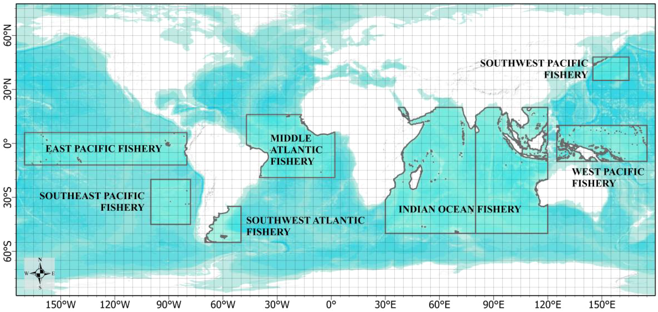
Distribution of fishing grounds for pelagic fisheries operations.
The Western Pacific (WP) fishery targets skipjack tuna, yellowfin tuna, bigeye tuna, and albacore tuna, with the study area ranging from 10°N to 10°S and 125°E to 175°E (Barclay and Cartwright, 2007; Wang et al., 2018).
The East Pacific (EP) fishery focuses on skipjack tuna and humboldt squid, with the study area ranging from 6°N to 12°S and 80°W to 170°W (Schaefer and Fuller, 2019; Fuller et al., 2021).
The Central Atlantic (CA) fishery, bigeye tuna, albacore tuna, and yellowfin tuna are the main catches. The study area ranging from 16°N to 19°S and 47°W to 2°E (Yang et al., 2015; Nóbrega et al., 2023).
The Southeast Pacific (SEP) fishery targets Chilean jack mackerel, jack mackerel and humboldt squid, with the study area ranging from 20°S to 45°S and 78°W to 100°W (Li et al., 2013, 2015).
The Southwest Atlantic (SWA) fishery, the primary focus is on squid species such as the Argentinean squid Illex argentinus and the Patagonian longfin squid. The study area ranging from 35°S to 55°S and 50°W to 70°W (Alemany et al., 2014; Wang et al., 2020).
The Northwest Pacific (NP) fishery, mackerel, pacific saury, Japanese sardine, Japanese anchovy, neon flying squid and jack mackerel are the main catches, with the study area ranging from 35°N to 48°N and 145°E to 165°E (Tseng et al., 2013; Li et al., 2024).
In the Indian Ocean fisheries, bigeye tuna, albacore tuna, yellowfin tuna, squid, and mackerel are the main catches. The study area ranging from 50°S to 20°N and 30°E to 120°E (Fu et al., 2023). The Indian Ocean was further divided into the West Indian Ocean (WIO) and East Indian Ocean (EIO) based on 80°E.
2.2 Data
To grape the trends of the marine environment, the OISST released by the National Oceanic and Atmospheric Administration (NOAA) of the United States is used in this paper, and the Oceanic Niño Index (ONI) developed by the Climate Prediction Center (CPC Footnote1) of NOAA as the representative of abnormal climatic events to describe the factors of ENSO teleconnection, as shown in Figure 2. An El Niño (La Niña) event is characterized by the average SST anomaly in the Nino 3.4 region for three consecutive months, i.e., the ONI is higher than 0.5°C (lower than -0.5°C) for five consecutive times (Glantz and Ramirez, 2020).
Figure 2
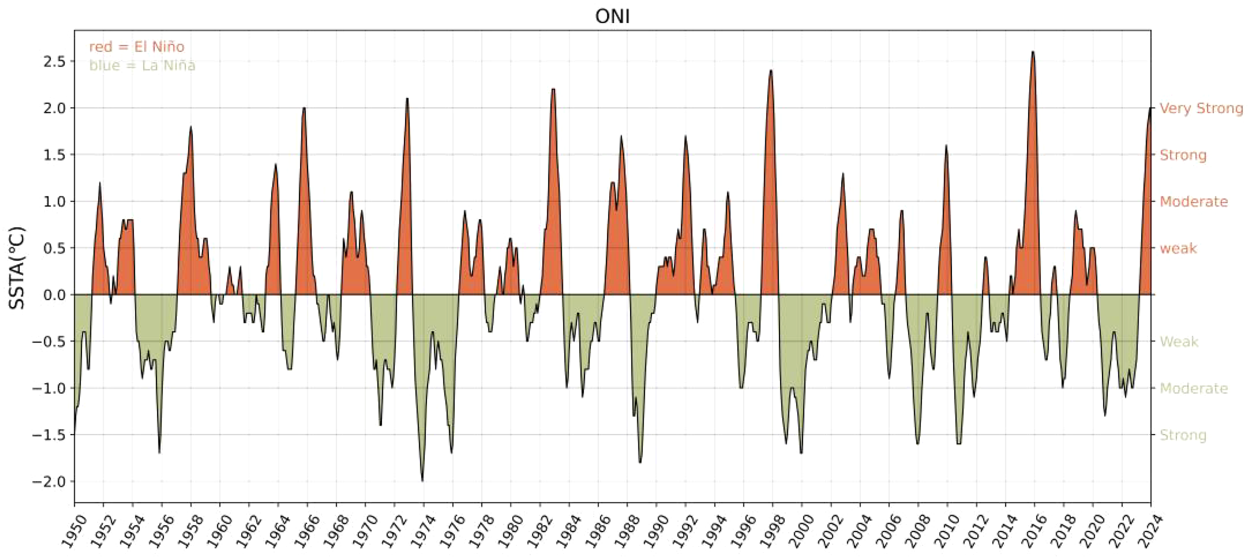
ONI index 1950-2024.
2.3 Seasonal and Trend decomposition using LOESS
As we all know, due to the Earth’s revolving around the sun and the angle of the ecliptic, natural phenomena on Earth usually exhibit natural rhythms of seasonal change. Therefore, when performing a long-term series analysis of climate change, the seasonal rhythm changes should be stripped. In this paper, the original SST time series is decomposed using STL (Seasonal-Trend decomposition using LOESS) to separate it into three components: seasonal component, trend component and residual component. STL is a widely used method for time series decomposition, in which LOESS (Locally Estimated Scatterplot Smoothing) is used to fit the trend and seasonality (Cleveland et al., 1990). Its decomposition can be expressed as Equation (1), STL decomposes a time series into three parts through iterative inner and outer loops. Internal circulation: de trending and separating seasonality and residual items; Seasonal smoothing extracts periodic components; Seasonal separation trend and residual items; Smooth updating of long-term trends. External loop: Calculate residual terms and assign lower weights to outliers; Combining weights to re smooth, optimize trends and seasonality. Where: is the original SST sequence; is the seasonal component; is the trend component; is the residual component. Taking the SST data in the western Pacific Ocean as an example, the seasonal component, trend component and residual component are decomposed from the original SST data using STL, and the trend component is extracted for further analysis, as shown in Figure 3a. Figure 3b shows the trend components extracted by STL in each fishing ground. Equation (2) is the measure of seasonality(FS). The FS is obtained by calculating the ratio of the variance of the residuals to the sum of the variances of the residual and seasonal components, and then subtracting this ratio from 1 (Wang et al., 2006). In the formula, Fsis the calculated seasonal strength of the time series, is the variance of the residuals, and is the sum of the variances of the residual and seasonal components. The value of seasonal strength index is between 0 and 1, and the closer it is to 1, the stronger the seasonality. Equation (3) is the measure of trend (FT). The calculation method of FT is similar to that of FS.
Figure 3
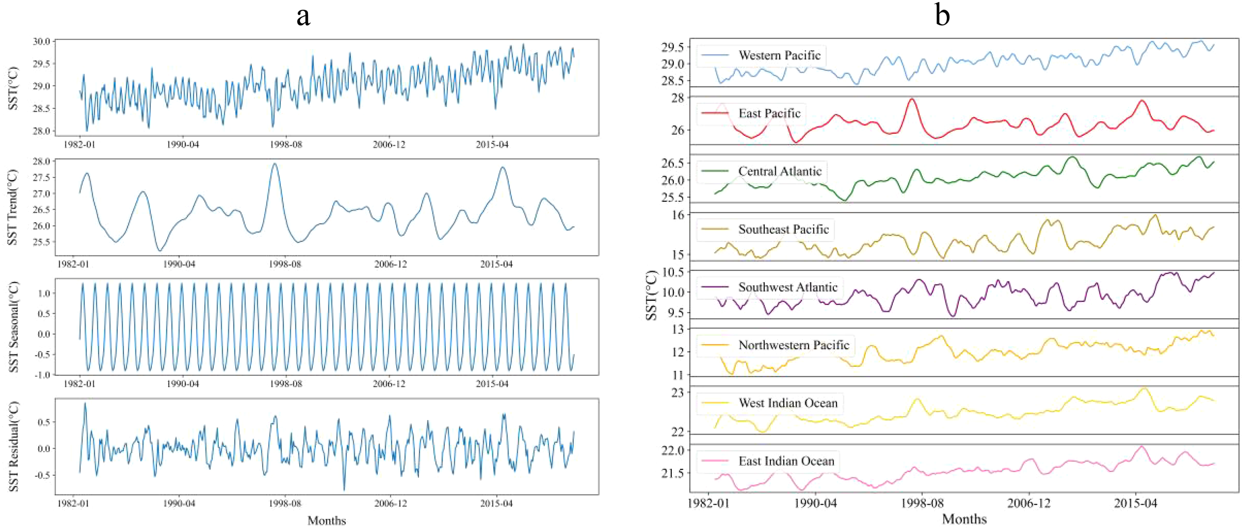
(a) STL decomposition of raw SST data in the Western Pacific; (b) Trend components of STL in each fishing ground.
2.4 Standard deviation and overall mean standard deviation
According to the scope of the fishing operating areas and corresponding SST data, the time series of the annual average SST in each fishing ground were calculated, and the relevant statistical characteristics (mean, standard deviation, maximum and minimum values) were calculated with a statistical unit per decade.
And meanwhile we calculated the overall mean SST for each grid point over 40 years as the climatic average state. In order to analyze the degree of dispersion of the SST per decade. relative to the 40-year climatic average state (), the overall mean SST for each grid point over 40 years was used as the mean in the standard deviation calculation formula to calculate the standard deviation for every 10 years, i.e. the overall mean standard deviation (OMSD). Equation (4) is the formula for calculating the overall mean standard deviation of SST, where OMSD is the overall mean standard deviation, is the monthly SST in time series i, is the average of the entire SST time series over 40 years, and N is the number of months in the calculated time period. Here N is equal to 120.
2.5 Fast Fourier transform
This paper uses the fast Fourier transform (FFT) to calculate the period of the trend component (Tt) time series. FFT is a commonly used signal analysis method, which has a wide range of applications in spectroscopy, geophysics, digital signal processing, and other fields. FFT can reflect the periodicity of a signal from frequency domain that cannot be reflected in time domain (M. et al., 2005; M. and M., 2019). So the FFT can be used to analyze the periodicity of SST time series. The principle is to first perform Fourier transform on the time series, then find the frequency corresponding to the maximum amplitude in the spectrum, and then calculate its reciprocal to obtain the period of the signal.The Fourier transform is shown in Equation (5), where X(k) is the k-th element of the complex result after the transformation, representing the frequency component in the frequency domain; x(n) is the n-th sample in the original time-domain signal; N is the total number of samples in the signal; i is the imaginary unit; and k is the index of the current frequency, ranging from 0 to N-1.
2.6 Pruned exact linear time
This paper uses the pruned exact linear time (PELT) method to do the detection of changepoints in the trend component of the SST time series, as shown in Equation (6):
where C(·) is the cost function and the penalty term, β is used to avoid fitting, y is the trend component of SST time series; τ is the vector of the change point locations; and m means the number of change points, with positions (Killick et al., 2012).
3 Result
3.1 Analysis of the change in the trend component of sea surface temperature every ten years
The mean value (), standard deviation (SD) and OMSD of the SST trend components for each of the eight fishing grounds per decade are calculated and shown in Tables 1–3.
Table 1
| Fishing grounds | (1982-1991) | Δ1 | (1992-2001) | Δ2 | (2002-2011) | Δ3 | (2012-2021) | |
|---|---|---|---|---|---|---|---|---|
| WP | 28.738 | 0.120 | 28.858 | 0.268 | 29.126 | 0.268 | 29.394 | 0.656 |
| EP | 26.245 | 0.044 | 26.289 | 0.022 | 26.311 | 0.226 | 26.537 | 0.292 |
| CA | 25.912 | -0.009 | 25.903 | 0.326 | 26.229 | 0.053 | 26.282 | 0.37 |
| SEP | 15.159 | 0.079 | 15.238 | 0.116 | 15.354 | 0.22 | 15.574 | 0.415 |
| SWA | 9.78 | 0.117 | 9.897 | 0.025 | 9.922 | 0.181 | 10.103 | 0.323 |
| NWP | 11.618 | 0.288 | 11.906 | 0.171 | 12.077 | 0.272 | 12.349 | 0.731 |
| WIO | 22.3 | 0.089 | 22.389 | 0.144 | 22.533 | 0.215 | 22.748 | 0.448 |
| EIO | 21.347 | 0.067 | 21.414 | 0.209 | 21.623 | 0.145 | 21.768 | 0.421 |
Mean and increment of the trend component of SST for each fishing ground per decade.
Table 2
| Fishing grounds | SD(1982-1991) | SD(1992-2001) | SD(2002-2011) | SD(2012-2021) |
|---|---|---|---|---|
| WP | 0.131 | 0.222 | 0.117 | 0.191 |
| EP | 0.631 | 0.585 | 0.361 | 0.475 |
| CA | 0.164 | 0.199 | 0.174 | 0.22 |
| SEP | 0.175 | 0.196 | 0.235 | 0.179 |
| SWA | 0.164 | 0.233 | 0.207 | 0.259 |
| NWP | 0.389 | 0.377 | 0.26 | 0.283 |
| WIO | 0.145 | 0.173 | 0.155 | 0.15 |
| EIO | 0.138 | 0.125 | 0.1 | 0.127 |
Standard deviation of SST per decade for each fishing ground.
Table 3
| Fishing grounds | OMSD(1982-1991) | OMSD(1992-2001) | OMSD(2002-2011) | OMSD(2012-2021) | OMSD(1982-2021) |
|---|---|---|---|---|---|
| WP | 0.319 | 0.28 | 0.152 | 0.412 | 0.305 |
| EP | 0.639 | 0.588 | 0.362 | 0.513 | 0.535 |
| CA | 0.235 | 0.267 | 0.228 | 0.298 | 0.259 |
| SEP | 0.244 | 0.217 | 0.237 | 0.303 | 0.252 |
| SWA | 0.219 | 0.235 | 0.207 | 0.314 | 0.247 |
| NWP | 0.536 | 0.385 | 0.275 | 0.459 | 0.423 |
| WIO | 0.241 | 0.201 | 0.161 | 0.297 | 0.229 |
| EIO | 0.235 | 0.176 | 0.132 | 0.263 | 0.207 |
| ONI | 0.918 | 0.949 | 0.792 | 0.813 | 0.871 |
OMSD of SST and ONI for each fishing ground (calculated using the mean value of the overall 40-year).
In Table 1 incremental quantity (Δ1, Δ2, Δ3) represents the difference (°C) between the mean SST values of eight pelagic fishing grounds during four time periods (1982-1991, 1992-2001, 2002-2011, 2012-2021) and the previous time period. The difference is calculated by subtracting the mean SST values of each time period. Respectively, Δ1 represents the increments of the from the period of 1982–1991 to the period of 1992-2001, Δ2 is the increment of the from the period of 1992–2001 to the period of 2002-2011, and Δ3 is the increment of the from the period of 2002–2011 to the period of 2012-2021.Δ is the total of Δ1 + Δ2 + Δ3, the overall change in the mean value of the SST trend component from 1982 to 2021.
To represent the changes of incremental quantity in SST, the stacked column chart of the mean changes in the SST trend components is plotted as Figure 4. From the total length of the column in Figure 4 and the Δ term of Table 1, it can be seen that the sea area with the most significant cumulative warming over the last 40 years is the Northwestern Pacific, followed by the Western Pacific, and then in turn next come the West Indian Ocean, the East Indian Ocean, the Southeast Pacific, the Central Atlantic,the Southwest Atlantic, and the East Pacific.
Figure 4
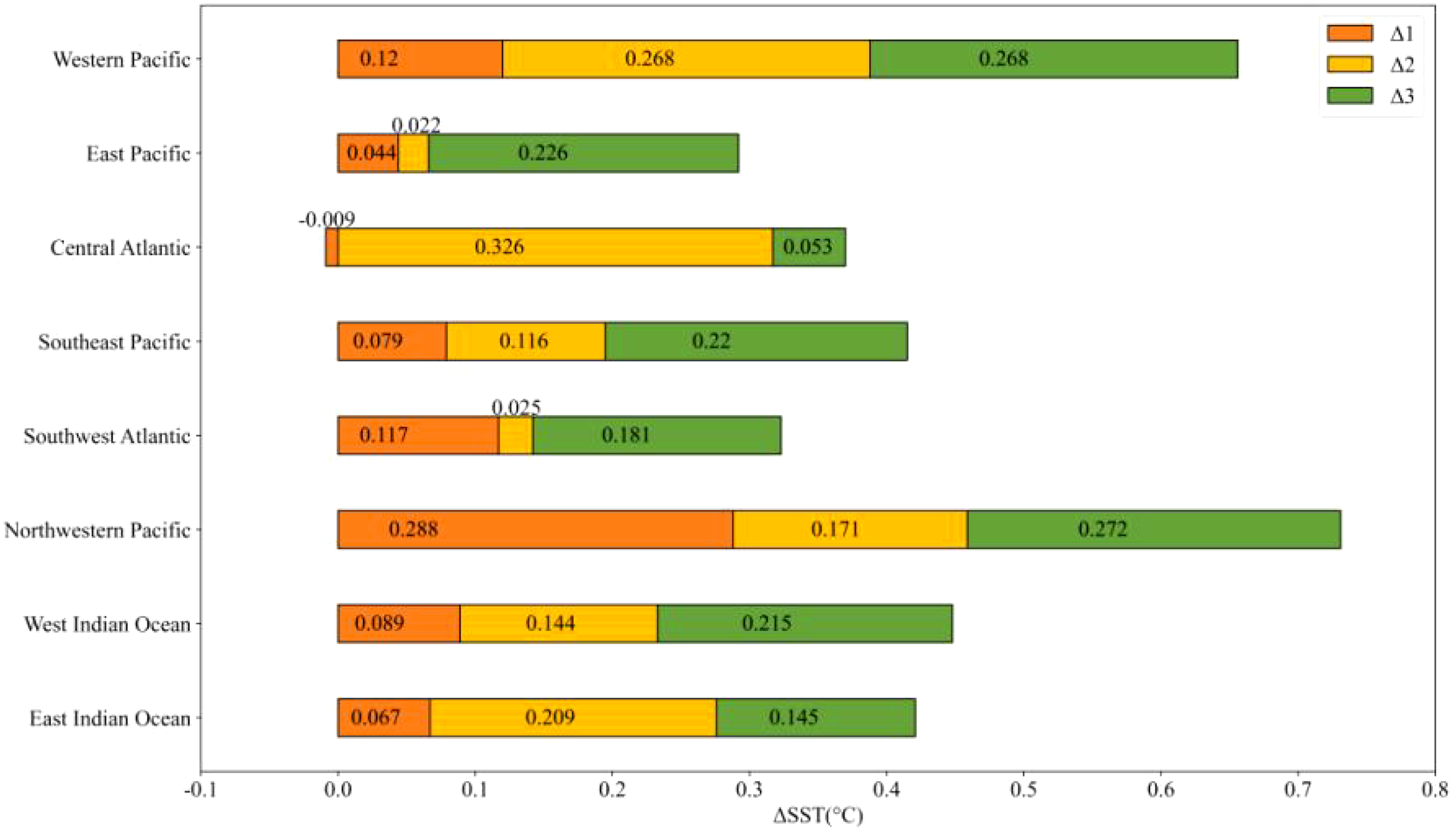
Stacked graph of mean changes in all fishing grounds.
Except for the Northwest Pacific, in all of the ocean areas Δ3 is greater than Δ1, and there are 5 regions (EP, SP, SWA, WP, and WIO) which Δ3 is the highest incremental quantity in decades, that means higher warming in the last two decades than in the previous two decade for most areas in the global oceans. But There are 2 areas (the CA and the EIO) that have the largest increases from the period of 1992–2001 to the period of 2002-2011. It is worth noting that, Δ1 of the CA is negative that means in the period of 1992–2001 is little lesser than the period of 1982-1991. And in all the fishing grounds the NP is the only region which Δ1 is highest increase that means compared to the other decades in the period of 1992–2001 has a very fast rise. These phenomena deserve great attention. Almost all the fishing ground in Pacific (except the NWP) had higher increases in the recent decade than in the previous two decades. The overall warming of the India Ocean is not very different, but the time interval of the fastest warming varies slightly. Warming in the WIO was higher in the last ten years than in the previous two decades (Δ3 is the highest, Δ3>Δ2>Δ1), and warming in the EIO was higher in the period of from 2002 to 2011 than in the other two decades, followed by the last ten years (Δ2 is the highest, Δ2>Δ3>Δ1).
Table 2 shows the SD, and Table 3 shows the OMSD of the SST trend components for each fishing ground per decade. From the SD of different time periods, people can know the fluctuations of data in a specific time period. From the OMSD of different time periods, we try to get how the data fluctuates relative to the climatic average state in a specific time period. Table 3 also gives both the whole OMSD from 1982 to 2021, which is the standard deviation in 40 years, and OMSD of ONI for different decades. As shown in Tables 2, 3, the first two highest values of SD and OMSD occur in the Western Pacific as well as the Northwestern Pacific in every decade, which means that these two areas have high short-term fluctuations in every 10 years even with respect to the climatic average state.
To identify possible patterns of change in time, we sorted the SDs and OMSDs for different time periods in each fishing ground, ① represents the period of from 1982 to 1991,② for from 1992 to 2001,③ for from 2002 to 2011 and ④ rom 2012 to 2021. The sorting results of the SDs and OMSDs for the eight sea regions is as shown in Table 4.
Table 4
| Fishing grounds | SD sorting results | OMSD sorting results |
|---|---|---|
| WP | ②>④>①>③ | ④>①>②>③ |
| EP | ①>②>④>③ | ①>②>④>③ |
| CA | ④>②>③>① | ④>②>①>③ |
| SEP | ③>②>④>① | ④>①>③>② |
| SWA | ④>②>③>① | ④>②>①>③ |
| NWP | ①>②>③>④ | ①>④>②>③ |
| WIO | ②>③>④>① | ④>①>②>③ |
| EIO | ①>④>②>③ | ②>①>④>③ |
Sorting results of SDs and OMSDs of eight fishing grounds.
Based on SD sorting results of each fishing ground at different periods, the differences and synchronicity of global ocean changes can be understood.For example, the SD values for the EP, NWP, and EIO of the first time period (1982-1991) reach the maximum value sorted in time, while they were at their minimum in the CA, SEP, SWA, and WIO, reflecting the great regional disparities in global sea temperature changes at this period. For the second time period (1992-2001), the SD values of five regions (EP, CA, SEP, SWA, and NWP) were the second highest value sorted in time, indicating that maybe there is a relative high degree of synchronicity of global ocean changes at this period.
According to OMSDs sorting results of each fishing ground at different periods, it is found that there are six of the eight fishing regions, the OMSD in the most recent decade is the highest among the four time periods. These regions are WP, CA, SEP, SWA, WIO, and EIO. This pattern generally aligns with the warming trend embodied by the increment of the SST average shown in Table 1 and Figure 4. There are seven of the eight fishing regions, the OMSD in the period from 2002 to 2011 is the lowest among the four time periods. This roughly means that the ocean during the period of 2002 to 2011 was closest to the average state of the global ocean over the past 40 years.
In order to more intuitively show the changes in the eight fishing grounds every decade, Figures 5–7. are box plots of SST per decade for the fishing grounds near the equator, the fishing grounds in the mid-latitude region, and the fishing grounds in the Indian Ocean. Box plots are statistical graphs used to describe the dispersion of a set of data. Box plots can reflect the stability of the optimization effect. The interquartile range (IQR) is used to measure the dispersion of data in box plots.
Figure 5
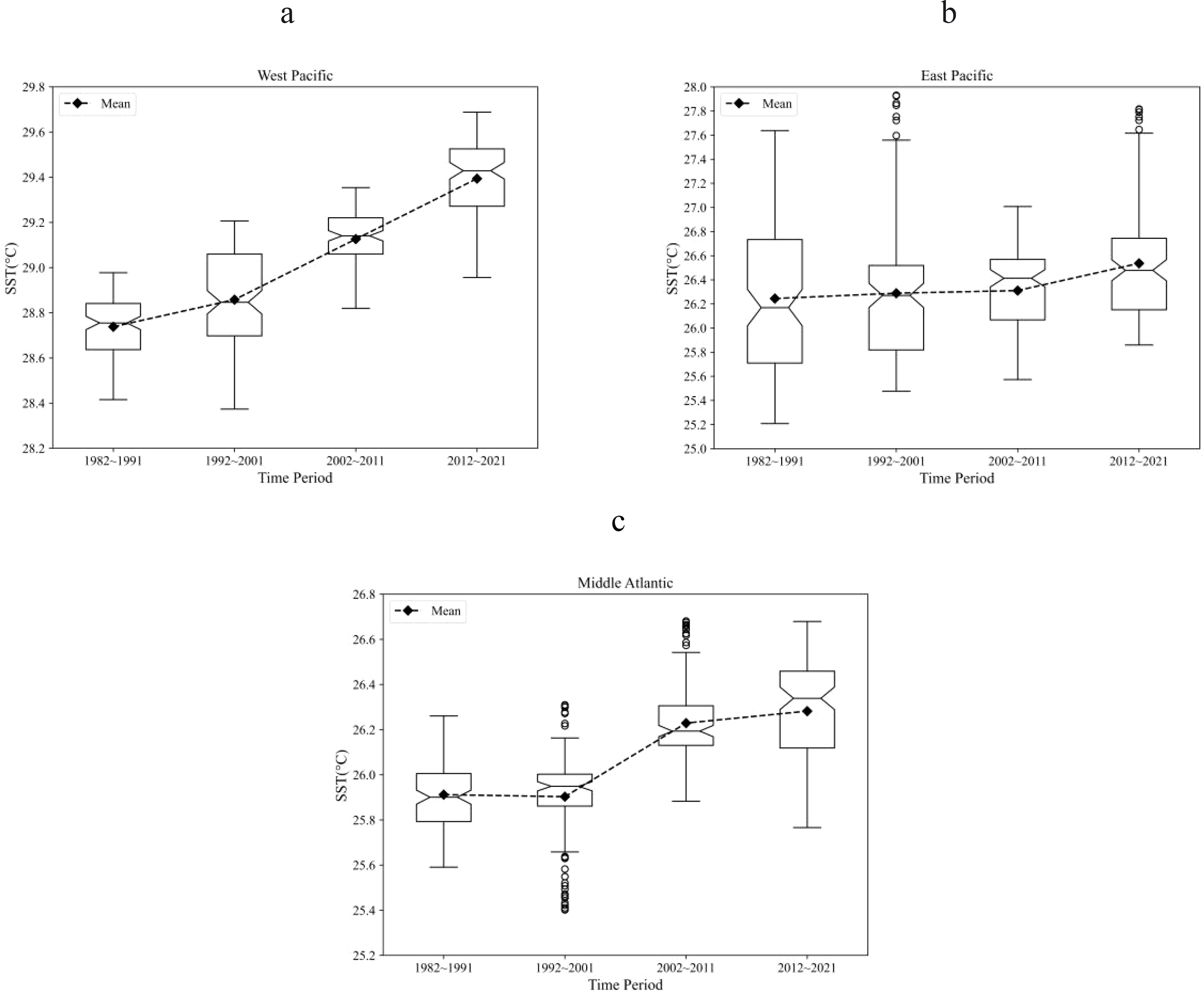
Box-plot of sea surface temperature per decade in fishing grounds near the equator. (a) WP; (b) EP; (c) CA.
Figure 6
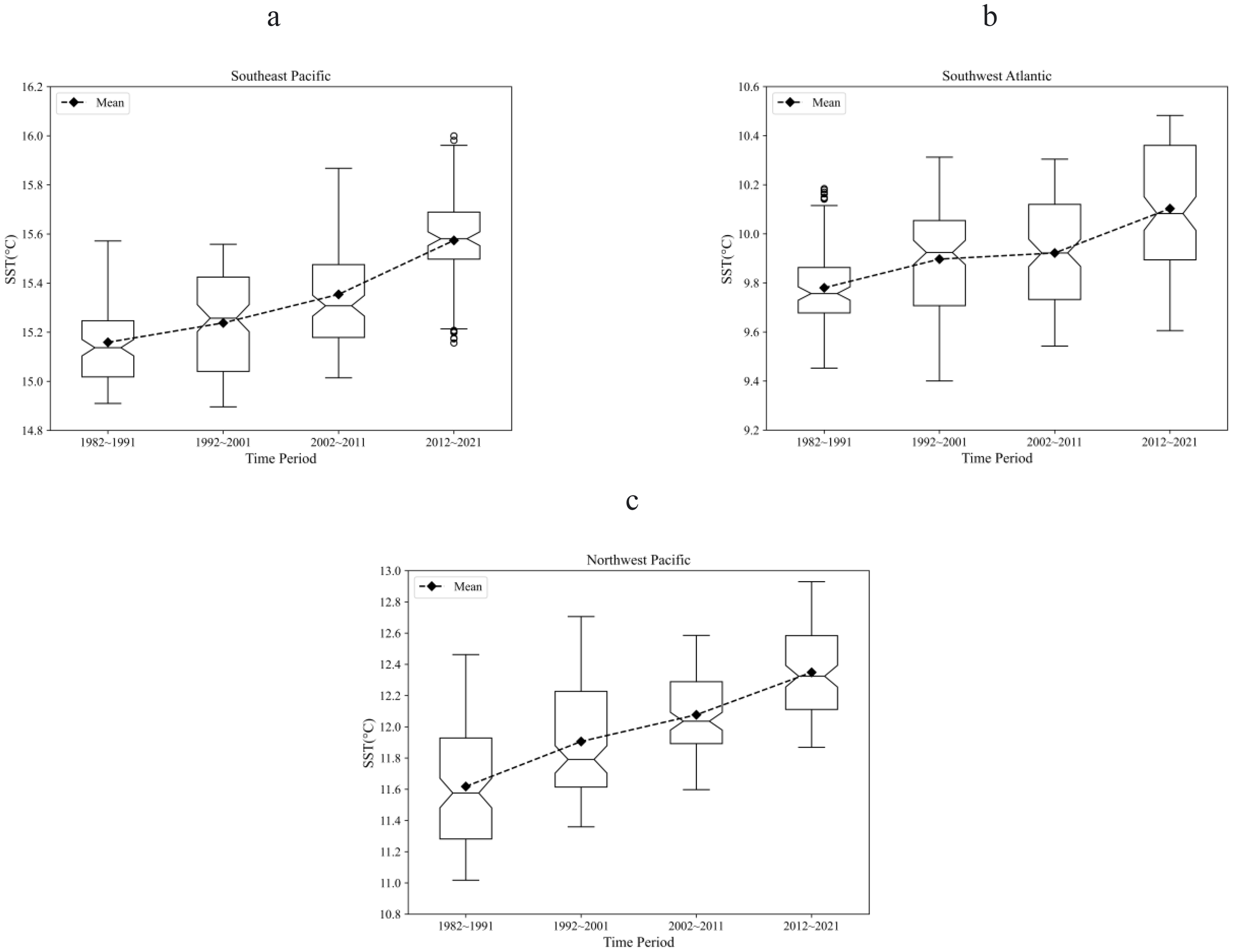
Box-plot of sea surface temperature per decade in fisheries in mid-latitudes (a) SEP; (b). SWA; (c) NWP.
Figure 7
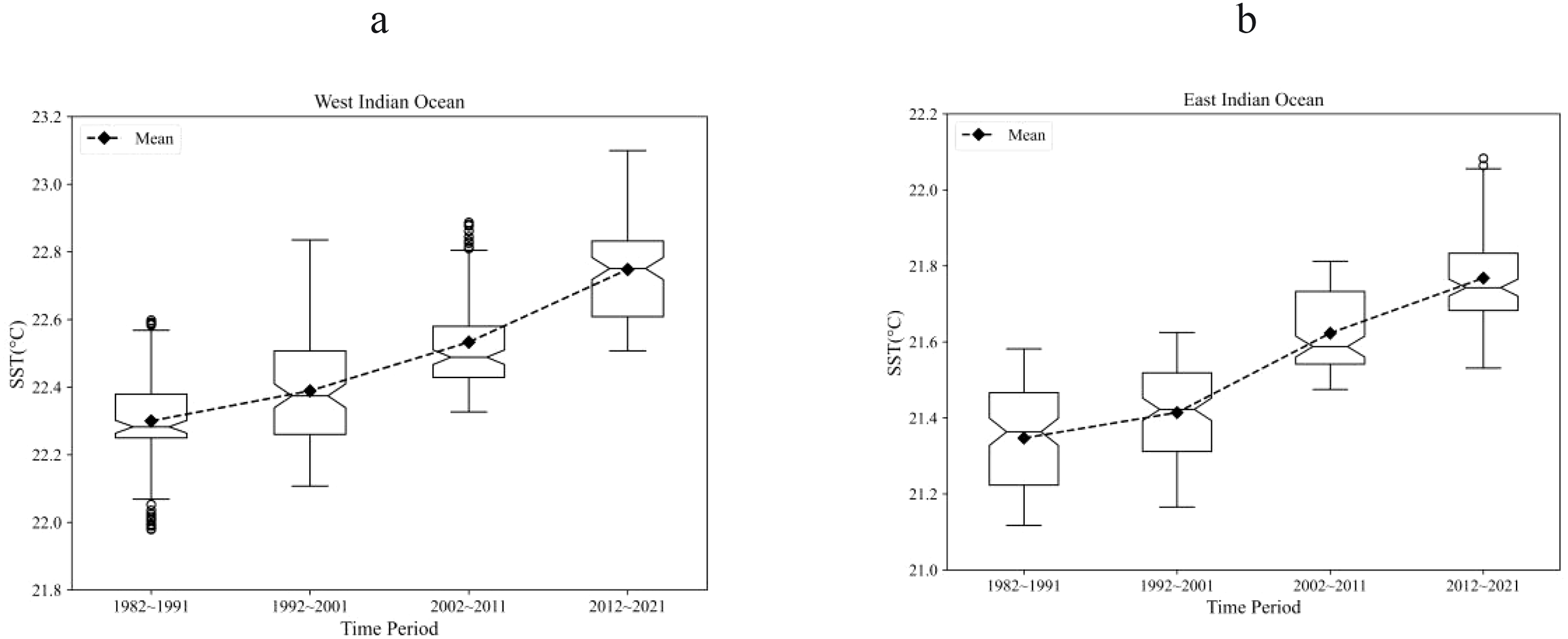
Box-plot of sea surface temperature per decade in Indian Ocean fisheries. (a) WIO; (b) EIO.
The SST in the WP continued to increase during these 40 years (Figure 5a). From 1982-1991, the SST range was 28.416°C to 28.977°C, increasing to 28.374°C to 29.206°C in 1992-2001, then narrowing to 28.82°C to 29.354°C in 2002-2011, and expanding again to 28.956°C to 29.688°C in 2012-2021. The interquartile ranges (IQR) for each decade were 0.204, 0.362, 0.16, and 0.253, indicating that SST fluctuations were consistent with changes in range.
The SST in the EP fisheries showed a slight upward trend during these four decades (Figure 5b). The IQR peaked at 1.024 in 1982-1991, then gradually decreased, with values of 0.7 in 1992-2001, 0.501 in 2002-2011, and 0.593 in 2012-2021. This indicates high variability, especially during 1982-1991, with SST data showing a right-skewed distribution.
The SST in the CA fisheries also showed a flat upward trend during these 40 years (Figure 5c), with greater fluctuations in 1982–1991 and 2012-2021, where IQRs were 0.213 and 0.34, respectively. In the middle decades (1992–2001 and 2002-2011), the IQRs were lower at 0.141 and 0.176. The data in 1992–2001 showed a left-skewed distribution, concentrating on lower values.
The SST value for the SEP fishery (Figure 6a) shows a clear upward trend, with IQR peaking at 0.385 in 1992-2001, then decreasing to 0.296 in 2002–2011 and 0.191 in 2012-2021. The data from 2012–2021 showed a left-skewed distribution, with higher values concentrated in the lower range.
The SST in the SWA fishery (Figure 6b) also showed a relatively stable upward trend, while the IQR was 0.185 in 1982-1991, increasing to 0.347 in 1992-2001, 0.388 in 2002-2011, and 0.467 in 2012-2021. The distribution in 1982–1991 was right-skewed, with lower values concentrated.
The upward trend of SST in the NWP fisheries (Figure 6c) is more significant than that in the SWA and SEP fisheries, and the overall IQR shows a decreasing trend, with the corresponding IQRs for the four decades being 0.646, 0.613, 0.397, and 0.473, respectively, indicating that the range of SST fluctuations is narrowing.
The SST of the WIO(Figure 7a) and the EIO(Figure 7b), both regions exhibited clear upward trends in SST. The IQR for WIO peaked at 0.247 during 1992-2001, while EIO’s IQR gradually decreased from 0.243 in 1982–1991 to 0.15 in 2012-2021, suggesting a narrowing fluctuation range. Overall, SST in WIO and EIO fisheries is relatively stable.
3.2 Seasonality and periodic analysis
3.2.1 Seasonality
Using formulas (2) and (3), the seasonal intensity index and trend intensity index were calculated to analyze the seasonality and trend of the SST time series. As shown in Table 5, the seasonal intensity of SST is very high in most of the regions over the 40 years, and the most affected by seasonality is the NWP, followed by the EIO, followed by the SEP, SWA, WIO, CA, EP and WP, respectively. The WP has the highest trend intensity (0.867), indicating a greater influence from long-term climate factors. Conversely, the SWA has the lowest trend intensity (0.538), suggesting a lower long-term climate impact compared to other areas.
Table 5
| Fishing grounds | Seasonal intensity index | Trend intensity index |
|---|---|---|
| WP | 0.774 | 0.867 |
| EP | 0.905 | 0.854 |
| CA | 0.964 | 0.824 |
| SEP | 0.989 | 0.609 |
| SWA | 0.987 | 0.538 |
| NWP | 0.994 | 0.666 |
| WIO | 0.980 | 0.849 |
| EIO | 0.992 | 0.81 |
Seasonal intensity indices of sea surface temperature for each fishery.
In most cases, the seasonal intensity index is higher than the trend intensity index, meaning seasonal changes dominate the SST variations in long-term trends. The NWP, EIO, and WIO exhibit strong seasonal fluctuations and relatively robust long-term trends, reflecting substantial impacts from both seasonal and long-term climate variations. In contrast, the SWA and SEP experience significant seasonal fluctuations but weaker long-term trends, suggesting that while seasonal factors heavily influence these areas, they are less affected by long-term climate changes. The WP shows the weakest seasonal variation but the strongest trend, indicating a gradual and stable increase in temperature over time with minimal seasonal fluctuations.
3.2.2 Periodic analysis
Table 6 shows the periodicity of SST and ONI (El Niño) series for each fishing ground. Although there are four in the Pacific Ocean, the periodicity of these four seas are not the same, and only the periodicity of EP and WP at low latitudes is exactly the same as that of ONI.
Table 6
| Fishing Grounds SST and ONI | Periodicity(year) |
|---|---|
| WP | 3.6 |
| EP | 5.6 |
| CA | 9.8 |
| SEP | 6.5 |
| SWA | 6.5 |
| NWP | 9.8 |
| WIO | 13.0 |
| EIO | 4.9 |
| ONI | 3.6 |
Periodicity of SST and ONI changes in each fishing ground.
Short-period fisheries: the WP have the same periodicity of 3.6 years, which is consistent with the ONI. The EIO has a slightly longer period of 4.9 years. The period of EP is slightly longer than that of EIO, at 5.6 years, which is still in the short-period range. Mid-period fisheries: the SEP and SWA both have a variability period of of 6.5 years, which lies between the short- and long-term, indicating that SST changes in these seas are influenced by short-term climatic phenomena as well as possibly from other medium-term climatic fluctuations. Long-period fisheries: The CA and NWP have longer periods of variability, both 9.8 years. This means that changes in SST in these areas may be influenced by long-term climate patterns and ocean circulation. The WIO has the longest period at 13.0 years, suggesting that SST changes in this region are significantly influenced by long-term climate changes and deep ocean dynamical processes. Periodicity and regional characteristics: The data in Table 6 show that there are significant differences in the period SST changes in different fishing grounds, which reflect the oceanic and atmospheric dynamics in different regions. The short cycles in the WP and EP coincide with the El Niño cycle, indicating that the response to El Niño in these regions is rapid and strong.
The continuous power spectra and corresponding significance levels of eight fishing grounds are shown in Figure 8.
Figure 8
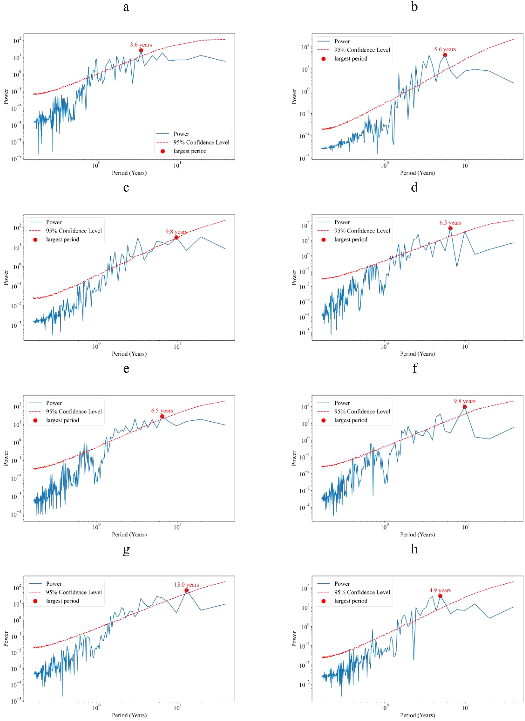
Continuous power spectra and corresponding significance levels of eight fishing grounds. (a) WP; (b) EP; (c) CA; (d) SEP; (e) SWA; (f) NWP; (g) WIO; (h) EIO.
3.2.3 Changepoint analysis by PELT
In this section, PELT changepoint detection method is applied to monitor the offline changepoints of the regional-scale annual mean SST time series. The years in which all the changepoints occurred were 1987, 1997, 2001, 2007, 2012, and 2017, but the number of changepoints in each fishing ground, except for the Indian Ocean, and the years of occurrence were not consistent (Figure 9).
Figure 9
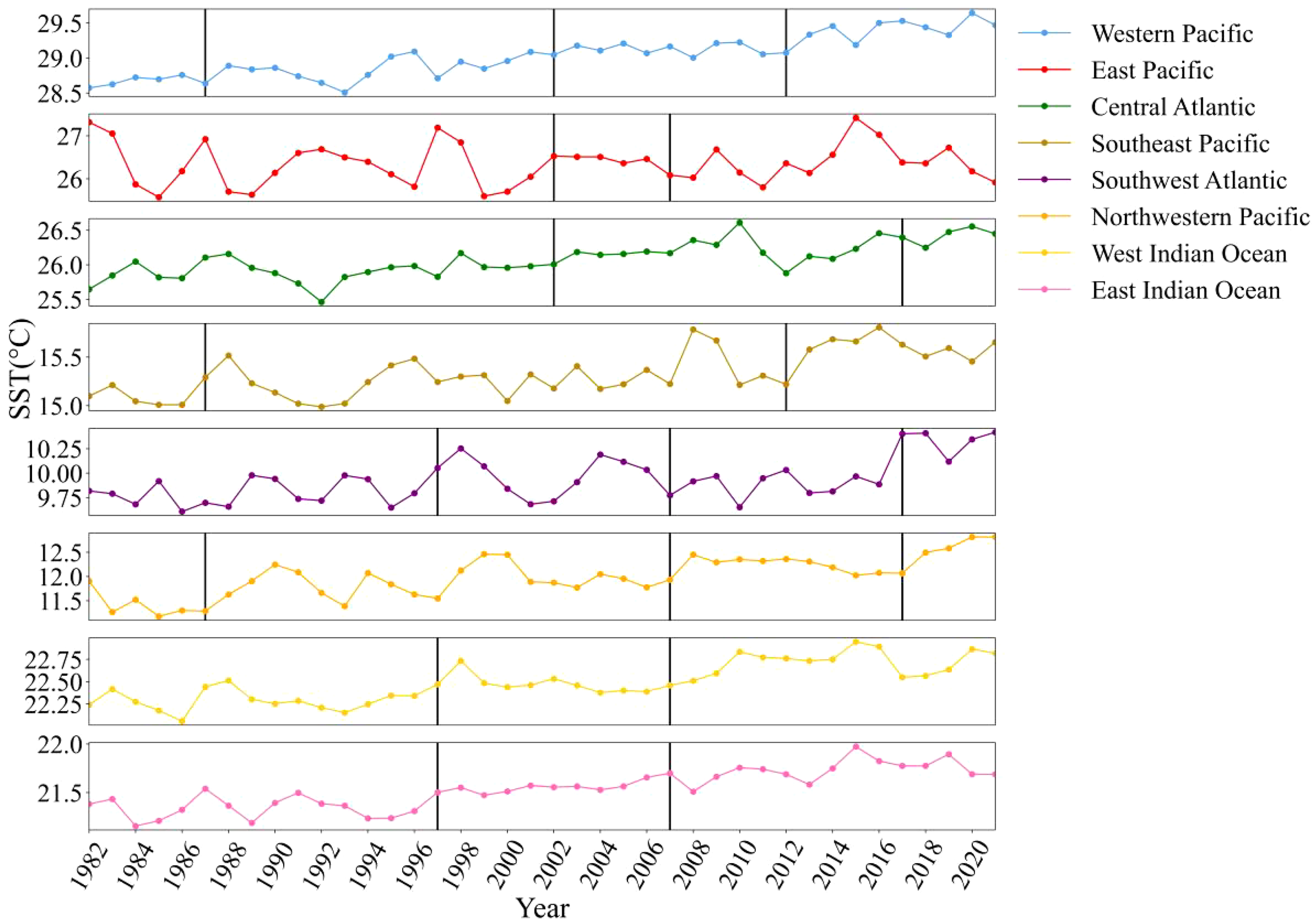
PELT change points for each fishing grounds.
The WP detected changepoints in 1997, 2002, and 2012. The EP exhibited changepoints in 2002 and 2017. The CA region also had changepoints in 2002 and 2017. In the SEP, changepoints were identified in 1987 and 2012. The SWA and NWP regions shared consistent changepoints in 1997, 2007, and 2017, yet their SST patterns diverged.
The WIO and EIO both experienced changepoints in 1997 and 2007, but exhibited differing patterns post-1997. The SWA, NWP, WIO, and EIO all had changepoints in 1997 and 2007, while the EP also detected a changepoint in 2007. Notably, 1997 corresponded with a super El Niño year and 2007 with a moderate La Niña year.
The NWP is affected by variations in and monsoon patterns related to El Niño and La Niña (Raj Deepak et al., 2019). Additionally, the WIO and EIO are sensitive to shifts in the Indian Ocean Dipole (IOD), which can be influenced by these climatic phenomena. The EP is directly impacted by El Niño, which can alter marine conditions.
4 Discussion
Based on the previous analysis, it can be found that despite the backdrop of global warming, the SST changes indifferent fishing grounds around the world still present a complex situation. There are many regional studies as follows.
For the Northwest Pacific fisheries, in the research spanning 35 years of Lim et al. (2017) from 1982 it is found that three super El Niño events have occurred historically, specifically during 1982-1983, 1997-1998, and 2015-2016 (Lim et al., 2017). In our study of a 40-year length from 1982 to 2021, which was analysed every 10 years, we found that SST exhibited a gradual increase in variability, particularly showing pronounced fluctuations during the second (1992-2001) and fourth decades (2012-2021). The IQR was notably larger during these periods. While the WP region displayed the weakest seasonal variation, it also showed the strongest overall warming trend, indicating a steady increase in temperature over time with minimal seasonal fluctuations. A change point was identified in the WP in 1997, coinciding with the super El Niño event of that year. Although WP detected only one corresponding change point, the timing of two of these super El Niño events coincides with significant fluctuations in WP.
For the East Pacific fisheries, Huang et al. (2024) conducted a 39 year study starting from 1980 and found that abnormal temperature fluctuations due to unusual climatic events can impact the abundance and distribution of fish species over time (Huang et al., 2024). For instance, Arkhipkin et al. (2014) found that temperature changes can influence the adult size and lifespan of species such as squid (Arkhipkin et al., 2014). Goñi et al. (2015) found that water temperature is the primary environmental variable that affects the spatiotemporal distribution changes of longfin tuna (Goñi et al., 2015). In our study significant fluctuations in SST were noted between 1982–1991 and 2012-2021, reflecting the region’s sensitivity to global climate change. Furthermore, change points were detected in 2002 and 2017, corresponding to a moderate El Niño in 2002 and a weak La Niña in 2017.
For the Central Atlantic fisheries, in the research spanning 35 years of Prigent et al. (2020) from 1982 it is found that the interannual variation of SST in the eastern equatorial Atlantic underwent a significant change around the year 2000, resulting in a 31% decrease in the SST change rate during the period from 2000 to 2017 (Prigent et al., 2020). This finding is consistent with the detection of a change point in the SST of the central Atlantic in 2002, and the reduction in the change rate indicates that SST variations became more gradual, with a decrease in temperature fluctuations. Similarly, in the CA fishery region, SST has remained relatively stable over the past four decades, characterized by a small interquartile range (IQR) and minimal variation. This stability has contributed to the maintenance of fish populations, supporting sustainable development. Significant changes were observed in 2002 and 2017, but compared to the other eight fishing grounds, the SST in the CA region remained relatively stable, consistently close to the median value.
For the Southeast Pacific fisheries, in the research spanning 35 years of Risaro et al. (2022) from 1982 it is found moderate to strong warming in the mid-latitude (30°-50°S) regions of the Southeast Pacific (Risaro et al., 2022). In our work, the SEP fishery found that SST has shown a gradual increase, with a large interquartile range (IQR) observed during 1992–2001 and abnormal outliers from 2012–2021, likely driven by the effects of the 2015 El Niño. Change points were identified in 1987 and 2012. Compared to other fishing grounds, the SST in the SEP exhibits strong seasonality, characterized by significant temperature fluctuations between warmer and cooler months. However, the overall trend of SST in the SEP remains relatively low.
For the Southwest Atlantic fisheries, in the research spanning 18 years of Rivas (2010) from 1985 it is found that the SST in the southwestern Atlantic exhibits a very distinct seasonal cycle (Rivas, 2010). In our research of 40 years we found that The SST fluctuations in the southwestern region studied in this article follow a clear seasonal pattern, but compared to other regions, the intensity of its long-term trend is relatively low, indicating that the influence of long-term climate factors is relatively small.
For the Northwest Pacific fisheries, in the research spanning 164 years of Wu et al. (2020) from 1854 it is found that over the past 164 years, sea temperatures in the northwest region have gradually increased, with an average rate of 0.033°C per decade (Wu et al., 2020). In line with this, the SST in the northwest Pacific fishery has also significantly increased, reaching its highest historical levels in the past decade. This upward trend further emphasizes the long-term and accelerating nature of sea temperature changes in the region.
In recent decades, WIO and EIO have also shown significant long-term warming trends, which interact with seasonal variations to produce complex SST changes. Mohan et al. (2021) analyzed SST data from 1900 to 2017 and found that the warming trend in the western and eastern Indian Ocean is largely caused by natural patterns of climate change (Mohan et al., 2021). Seasonal intensity has a significant impact on both WIO and EIO, and SST fluctuations are driven by different seasonal cycles, which are particularly prominent in these regions due to the influence of monsoon changes and trade winds. Li et al. (2017) analyzed SST data from 1955 to 2015 and found that the SST variability in the tropical Indian Ocean exhibits a hundred year warming trend combined with interannual and ten-year variations (Li et al., 2017). And the rapid warming trend during the period of 2003-2013, which is consistent with the higher warming of EIO in our article from 2002 to 2012 compared to other time periods.
Our analysis of SST variability across eight pelagic fishing grounds reveals distinct temporal scales in the Pacific, Atlantic, and Indian Oceans, aligning closely with findings from global SST studies, notably Bulgin et al. using 37 years of satellite SST data (1981-2018), Bulgin et al. demonstrated that equatorial Pacific SST variability is dominated by 1-5-year cycles driven by the ENSO, with a maximum variance of 1.9 K² (Bulgin et al., 2020). This is consistent with our findings in the NWP and WP fishing grounds, where FFT analysis identifies 3.7-year cycles as the primary mode of variability.
Although the OISST dataset (0.25° resolution) provides strong global SST coverage, its spatial resolution may not fully capture fine scale SST variations, such as ocean fronts and eddies (Xing et al., 2023; Belkin, 2021; Xing et al., 2024), which are crucial for fisheries in regions. This limitation may underestimate the local changes associated with fish population dynamics. Higher resolution datasets can address this issue in future research (Embury et al., 2024).
Overall, while all fisheries show a warming trend, regional differences exist in the extent and volatility of SST changes, influenced by geography, ocean circulation, and climatic events like El Niño/La Niña (Lu et al., 2001; Turk et al., 2001). These differences highlight the need for further study on the impact of SST variability on fisheries resources (Zhou et al., 2022).
5 Conclusion
In conclusion, the analysis of SST trends over the past four decades reveals significant regional variability across the eight fishing grounds studied. The Northwestern Pacific shows the most pronounced warming, followed by the Western Pacific and the West Indian Ocean, with other regions experiencing lesser but notable increases. The incremental changes in SST, particularly Δ3, demonstrate that most regions, except for the Northwest Pacific, have experienced higher warming in the past two decades compared to earlier periods, indicating an accelerating trend in oceanic warming.
The SD and OMSD further emphasize the complexity of SST variability. While SD rankings show no clear pattern, OMSD rankings suggest that six of the eight regions have seen their highest variability in the most recent decade. This increasing variability aligns with the broader warming trends and points to region-specific responses to global climate influences, particularly in areas like the Western Pacific, Central Atlantic, and Southwest Atlantic.
The box plots and IQR highlight both the upward trends in SST and the varying levels of stability across the fishing grounds. Regions like the WP, WIO and EIO exhibit relatively stable patterns, while areas such as the EP and SWA display greater fluctuations. Periodicity analyses indicate that SST variability in different regions correlates with both short-term cycles, such as the ENSO, and long-term oceanic patterns like the AMO and IOD.
Finally, change-point analysis using the PELT method underscores the influence of significant climatic events on SST trends. The alignment of change points in 1997, 2007, and 2017 across multiple regions correlates with major El Niño and La Niña episodes, further illustrating the critical role of these phenomena in shaping SST dynamics. The findings highlight the intricate interplay between oceanic and atmospheric processes, and the growing impact of climate change on global fisheries, calling for continued monitoring and adaptive management strategies.
Statements
Data availability statement
Publicly available datasets were analyzed in this study. This data can be found here: https://www.psl.noaa.gov/data/gridded/data.noaa.oisst.v2.highres.html.
Author contributions
WZ: Conceptualization, Data curation, Formal Analysis, Funding acquisition, Methodology, Project administration, Resources, Supervision, Writing – original draft, Writing – review & editing. QL: Software, Validation, Visualization, Writing – original draft.
Funding
The author(s) declare that financial support was received for the research and/or publication of this article. This work was financially supported by the National Key R&D Program of China (No. 2023YFD2401303), and the Central Public-Interest Scientific Institution Basal Research Fund, ECSFR, CAFS (No. 2022ZD0402).
Conflict of interest
The authors declare that the research was conducted in the absence of any commercial or financial relationships that could be construed as a potential conflict of interest.
Generative AI statement
The author(s) declare that no Generative AI was used in the creation of this manuscript.
Publisher’s note
All claims expressed in this article are solely those of the authors and do not necessarily represent those of their affiliated organizations, or those of the publisher, the editors and the reviewers. Any product that may be evaluated in this article, or claim that may be made by its manufacturer, is not guaranteed or endorsed by the publisher.
References
1
Abbass K. Qasim M. Z. Song H. Murshed M. Mahmood H. Younis I. (2022). A review of the global climate change impacts, adaptation, and sustainable mitigation measures. Environ. Sci. pollut. Res.29, 42539–42559. doi: 10.1007/s11356-022-19718-6
2
Alemany D. Acha E. M. Iribarne O. O. (2014). Marine fronts are important fishing areas for demersal species at the argentine sea (southwest atlantic ocean). J. Sea Res.87, 56–67. doi: 10.1016/j.seares.2013.12.006
3
Antão L. H. Bates A. E. Blowes S. A. Waldock C. Supp S. R. Magurran A. E. et al . (2020). Temperature-related biodiversity change across temperate marine and terrestrial systems. Nat. Ecol. Evol.4, 927–933. doi: 10.1038/s41559-020-1185-7
4
Arkhipkin A. Argüelles J. Shcherbich Z. Yamashiro C. (2014). Ambient temperature influences adult size and life span in jumbo squid (dosidicus gigas). Can. J. Fish Aquat Sci.72, 400–409. doi: 10.1139/cjfas-2014-0386
5
Barclay K. Cartwright I. (2007). Governance of tuna industries: the key to economic viability and sustainability in the western and central pacific ocean. Mar. Policy31, 348–358. doi: 10.1016/j.marpol.2006.09.007
6
Belkin I. M. (2021). Remote sensing of ocean fronts in marine ecology and fisheries. Remote Sens.13, 883. doi: 10.3390/rs13050883
7
Brulé T. Renán X. Colás-Marrufo T. (2022). Potential impact of climate change on fish reproductive phenology: a case study in gonochoric and hermaphrodite commercially important species from the southern gulf of Mexico. Fishes7, 156. doi: 10.3390/fishes7040156
8
Bulgin C. E. Merchant C. J. Ferreira D. (2020). Tendencies, variability and persistence of sea surface temperature anomalies. Sci. Rep.10, 7986. doi: 10.1038/s41598-020-64785-9
9
Chemshirova I. Hoving H. Arkhipkin A. (2021). Temperature effects on size, maturity, and abundance of the squid illex argentinus (cephalopoda, ommastrephidae) on the patagonian shelf. Estuarine Coast. Shelf Sci.255, 107343. doi: 10.1016/j.ecss.2021.107343
10
Cleveland R. B. Cleveland W. S. Mcrae J. E. Terpenning I. (1990). Stl: a seasonal-trend decomposition procedure based on loess (with discussion). J. Off Stat.6, 3–73.
11
Cubillos L. A. Paramo J. Ruiz P. Núñez S. Sepúlveda A. (2008). The spatial structure of the oceanic spawning of jack mackerel (trachurus murphyi) off central Chile, (1998–2001). Fish Res.90, 261–270. doi: 10.1016/j.fishres.2007.10.016
12
Dizon A. E. Neill W. H. Magnuson J. J. (1977). Rapid temperature compensation of volitional swimming speeds and lethal temperatures in tropical tunas (scombridae). Environ. Biol. Fishes2, 83–92. doi: 10.1007/BF00001418
13
Embury O. Merchant C. J. Good S. A. Rayner N. A. Høyer J. L. Atkinson C. et al . (2024). Satellite-based time-series of sea-surface temperature since 1980 for climate applications. Sci. Data11, 326. doi: 10.1038/s41597-024-03147-w
14
Fox-Kemper B. Hewitt H. T. Xiao C. Aðalgeirsdóttir G. Drijfhout S. S. Edwards T. L. et al . (2021). “2021: ocean, cryosphere and sea level change,” in Climate Change 2021 – The Physical Science Basis: Working Group I Contribution to the Sixth Assessment Report of the Intergovernmental Panel on Climate Change. Eds. Masson-DelmotteV.ZhaiP.PiraniA.ConnorsS. L.PéanC.BergerS.CaudN.ChenY.GoldfarbL.GomisM. I.HuangM.LeitzellK.LonnoyE.MatthewsJ. B. R.MaycockT. K.WaterfieldT.YelekçiO.YuR. (Cambridge, United Kingdom and New York, NY, USA: Cambridge University Press), 1211–1362. doi: 10.1017/9781009157896.011
15
Fu D. Debruyn P. Fiorellato F. Nelson L. Pierre L. FernandezDiaz C. et al . (2023). Assessing the impact of growth on estimates of fishing mortality — an illustration with Indian ocean bigeye tuna. Reg. Stud. Mar. Sci.62, 102981. doi: 10.1016/j.rsma.2023.102981
16
Fuller L. Griffiths S. Olson R. Galván-Magaña F. Bocanegra-Castillo N. Alatorre-Ramírez V. (2021). Spatial and ontogenetic variation in the trophic ecology of skipjack tuna, katsuwonus pelamis, in the eastern pacific ocean. Mar. Biol.168, 73. doi: 10.1007/s00227-021-03872-5
17
Glantz M. H. Ramirez I. J. (2020). Reviewing the oceanic niño index (oni) to enhance societal readiness for el niño’s impacts. Int. J. Disaster Risk Sci.11, 394–403. doi: 10.1007/s13753-020-00275-w
18
Goñi N. Didouan C. Arrizabalaga H. Chifflet M. Arregui I. Goikoetxea N. et al . (2015). Effect of oceanographic parameters on daily albacore catches in the northeast atlantic. Deep Sea Res. Part II: Topical Stud. Oceanography113, 73–80. doi: 10.1016/j.dsr2.2015.01.012
19
Hendrix C. S. Glaser S. M. Lambert J. E. Roberts P. M. (2022). Global climate, el niño, and militarized fisheries disputes in the east and south China seas. Mar. Policy143, 105137. doi: 10.1016/j.marpol.2022.105137
20
Huang M. Chen Y. Zhou W. Wei F. (2024). Assessing the response of marine fish communities to climate change and fishing. Conserv. Biol.38), e14291. doi: 10.1111/cobi.14291
21
Kang B. Pecl G. T. Lin L. Sun P. Zhang P. Li Y. et al . (2021). Climate change impacts on China’s marine ecosystems. Rev. Fish Biol. Fish31, 599–629. doi: 10.1007/s11160-021-09668-6
22
Killick R. Fearnhead P. Eckley I. A. (2012). Optimal detection of changepoints with a linear computational cost. J. Am. Stat. Assoc.107, 1590–1598. doi: 10.1080/01621459.2012.737745
23
Klein S. A. Soden B. J. Lau N. (1999). Remote sea surface temperature variations during ENSO: evidence for a tropical atmospheric bridge. J. Climate12, 917–932. doi: 10.1175/1520-0442(1999)012<0917:RSSTVD>2.0.CO;2
24
Kumar P. S. Pillai G. N. Manjusha U. (2014). El Nino Southern Oscillation (ENSO) impact on tuna fisheries in Indian Ocean. SpringerPlus3, 591. doi: 10.1186/2193-1801-3-591
25
Lam V. W. Y. Allison E. H. Bell J. D. Blythe J. Cheung W. W.L. Frölicher T. L. et al . (2020). Climate change, tropical fisheries and prospects for sustainable development. Nat. Rev. Earth Environ.1, 440–454. doi: 10.1038/s43017-020-0071-9
26
Lee C. W. Tseng Y. H. Sui C. H. Zheng F. Wu E. T. (2020). Characteristics of the prolonged El Niño events during 1960–2020. Geophys. Res. Lett.47, e2020GL088345. doi: 10.1029/2020GL088345
27
Lehodey P. Alheit J. Barange M. Baumgartner T. Beaugrand G. Drinkwater K. et al . (2006). Climate variability, fish, and fisheries. J. Clim19, 5009–5030. doi: 10.1175/JCLI3898.1
28
Li G. Cao J. Zou X. Chen X. Runnebaum J. (2015). Modeling habitat suitability index for Chilean jack mackerel (trachurus murphyi) in the south east pacific. Fish Res.178, 47–60. doi: 10.1016/j.fishres.2015.11.012
29
Li Y. Han W. Zhang L. (2017). Enhanced decadal warming of the southeast Indian ocean during the recent global surface warming slowdown. Geophys Res. Lett.44, 9876–9884. doi: 10.1002/2017GL075050
30
Li W. Zhang C. Liu Y. Liu S. Tian H. Cao C. et al . (2024). Different growth patterns reveal the potential origins of two pacific saury (cololabis saira) groups in the northwest pacific ocean. Fish Res.272, 106933. doi: 10.1016/j.fishres.2023.106933
31
Li G. Zou X. Chen X. Zhou Y. Zhang M. (2013). Standardization of cpue for Chilean jack mackerel (trachurus murphyi) from chinese trawl fleets in the high seas of the southeast pacific ocean. J. Ocean Univ China12, 441–451. doi: 10.1007/s11802-013-1987-1
32
Lim Y. -K. Kovach R. M. Pawson S. Vernieres G. (2017). The 2015/16 el niño event in context of the merra-2 reanalysis: a comparison of the tropical pacific with 1982/83 and 1997/98. J. Clim30, 4819–4842. doi: 10.1175/JCLI-D-16-0800.1
33
Lin D. Chen X. Wei Y. Chen Y. (2017). The energy accumulation of somatic tissue and reproductive organs in post-recruit female Illex argentinus and the relationship with sea surface oceanography. Fisheries Res.185, 102–114. doi: 10.1016/j.fishres.2016.09.023
34
Lu H. -J. Lee K. -T. Lin H. -L. Liao C. -H. (2001). Spatio-temporal distribution of yellowfin tuna thunnus albacares and bigeye tuna thunnus obesus in the tropical pacific ocean in relation to large-scale temperature fluctuation during enso episodes. Fish Sci.67, 1046–1052. doi: 10.1046/j.1444-2906.2001.00360.x
35
M. Y. Y. M. M. C. (2019). “Developing fast techniques for periodicity analysis of time series,” in 2019 3rd International Symposium on Multidisciplinary Studies and Innovative Technologies (ISMSIT) (IEEE, Ankara, Turkey), 1–5.
36
M. G. E. W. G. A. A. K. E. (2005). Periodicity detection in time series databases. IEEE Trans. Knowl. Data Eng.17, 875–887. doi: 10.1109/TKDE.2005.114
37
Mohan S. Mishra S. K. Sahany S. Behera S. (2021). Long-term variability of sea surface temperature in the tropical Indian ocean in relation to climate change and variability. Glob Planet Change199, 103436. doi: 10.1016/j.gloplacha.2021.103436
38
Nóbrega M. F. de Lira M. G. Oliveira M. A. Oliveira J. E. L. (2023). Interactions between oceanographic variables and population structure of the yellowfin tuna (bonnaterre 1788) in the western central atlantic. Fish Oceanogr32, 213–228. doi: 10.1111/fog.12624
39
Overland J. E. Alheit J. Bakun A. Hurrell J. W. Mackas D. L. Miller A. J. (2010). Climate controls on marine ecosystems and fish populations. J. Mar. Syst.79, 305–315. doi: 10.1016/j.jmarsys.2008.12.009
40
Prigent A. Lübbecke J. F. Bayr T. Latif M. Wengel C. (2020). Weakened sst variability in the tropical atlantic ocean since 2000. Clim Dyn54, 2731–2744. doi: 10.1007/s00382-020-05138-0
41
Raj Deepak S. N. Chowdary J. S. Dandi A. R. Srinivas G. Parekh A. Gnanaseelan C. et al . (2019). Impact of multiyear La Niña events on the South and East Asian summer monsoon rainfall in observations and CMIP5 models. Clim Dyn52, 6989–7011. doi: 10.1007/s00382-018-4561-0
42
Risaro D. B. Chidichimo M. P. Piola A. R. (2022). Interannual variability and trends of sea surface temperature around southern south america. Front. Mar. Sci.9. doi: 10.3389/fmars.2022.829144
43
Rivas A. L. (2010). Spatial and temporal variability of satellite-derived sea surface temperature in the southwestern atlantic ocean. Cont Shelf Res.30, 752–760. doi: 10.1016/j.csr.2010.01.009
44
Schaefer K. Fuller D. (2019). Spatiotemporal variability in the reproductive dynamics of skipjack tuna (katsuwonus pelamis) in the eastern pacific ocean. Fish Res.209, 1–13. doi: 10.1016/j.fishres.2018.09.002
45
Shaw T. A. Arblaster J. M. Birner T. Butler A. H. Domeisen D. I. V. Garfinkel C. I. et al . (2024). Emerging climate change signals in atmospheric circulation. AGU Adv.5, e2024AV001297. doi: 10.1029/2024AV001297
46
Stuart-Smith R. D. Edgar G. J. Bates A. E. (2017). Thermal limits to the geographic distributions of shallow-water marine species. Nat. Ecol. Evol.1, 1846–1852. doi: 10.1038/s41559-017-0353-x
47
Tseng C.-T. Su N.-J. Sun C.-L. Punt A. E. Yeh S.-Z. Liu D.-C. et al . (2013). Spatial and temporal variability of the pacific saury (cololabis saira) distribution in the northwestern pacific ocean. Ices J. Mar. Sci.70, 991–999. doi: 10.1093/icesjms/fss205
48
Turk D. McPhaden M. J. Busalacchi A. J. Lewis M. R. (2001). Remotely sensed biological production in the equatorial pacific. Science293, 471–474. doi: 10.1126/science.1056449
49
Vásquez S. Correa-Ramírez M. Parada C. Sepúlveda A. (2013). The influence of oceanographic processes on jack mackerel (trachurus murphyi) larval distribution and population structure in the southeastern pacific ocean. Ices J. Mar. Sci.70, 1097–1107. doi: 10.1093/icesjms/fst065
50
Vergés A. McCosker E. Mayer-Pinto M. Coleman M.A. Wernberg T. Ainsworth T. et al . (2019). Tropicalisation of temperate reefs: implications for ecosystem functions and management actions. Funct. Ecol.33, 1000–1013. doi: 10.1111/fec.2019.33.issue-6
51
Wang J. Chen X. Staples K. W. Chen Y. (2018). The skipjack tuna fishery in the west-central pacific ocean: applying neural networks to detect habitat preferences. Fish Sci.84, 1–13. doi: 10.1007/s12562-017-1161-6
52
Wang C. Fiedler P. (2006). Enso variability and the eastern tropical pacific: a review. Prog. Oceanogr69, 239–266. doi: 10.1016/j.pocean.2006.03.004
53
Wang J. Jiang Y. Zhang J. Xinjun C. Kitazawa D. (2020). Catch per unit effort (cpue) standardization of argentine shortfin squid (illex argentinus) in the southwest atlantic ocean using a habitat-based model. Int. J. Remote Sens41, 9309–9327. doi: 10.1080/01431161.2020.1798550
54
Wang X. Smith K. Hyndman R. (2006). Characteristic-based clustering for time series data. Data Min Knowl. Discovery13, 335–364. doi: 10.1007/s10618-005-0039-x
55
Wu Z. Jiang C. Conde M. Chen J. Deng B. (2020). The long-term spatiotemporal variability of sea surface temperature in the northwest pacific and China offshore. Ocean Sci.16, 83–97. doi: 10.5194/os-16-83-2020
56
Xing Q. Yu H. Wang H. (2024). Global mapping and evolution of persistent fronts in Large Marine Ecosystems over the past 40 years. Nat. Commun.15, 4090. doi: 10.1038/s41467-024-48566-w
57
Xing Q. Yu H. Wang H. Ito S.-i. Chai F. (2023). Mesoscale eddies modulate the dynamics of human fishing activities in the global midlatitude ocean. Fish Fisheries24, 527–543. doi: 10.1111/faf.12742
58
Yang S. L. Jin S. F. Hua C. J. Dai Y. (2015). spatial-temporal distribution of bigeye tuna thunnus obesus in the tropical atlantic ocean based on argo data. Ying Yong Sheng Tai Xue Bao26, 601–608.
59
Zhai P. Zhou B. Chen Y. (2018). A review of climate change attribution studies. J. Meteorol Res.32, 671–692. doi: 10.1007/s13351-018-8041-6
60
Zhou W. Hu H. Fan W. Jin S. (2022). Impact of abnormal climatic events on the cpue of yellowfin tuna fishing in the central and western pacific. Sustainability14 (3), 1217. doi: 10.3390/su14031217
Summary
Keywords
pelagic fisheries, sea surface temperature, Ocean Nino Index, trend decomposition, variance analysis, the interquartile ranges, change point analysis
Citation
Lai Q and Zhou W (2025) Multiscale variation analysis of sea surface temperature in the fishing grounds of pelagic fisheries. Front. Mar. Sci. 12:1567030. doi: 10.3389/fmars.2025.1567030
Received
26 January 2025
Accepted
19 May 2025
Published
10 June 2025
Volume
12 - 2025
Edited by
Jorge Paramo, University of Magdalena, Colombia
Reviewed by
Hao Tian, Ocean University of China, China
Qinwang Xing, Shanghai Ocean University, China
Updates
Copyright
© 2025 Lai and Zhou.
This is an open-access article distributed under the terms of the Creative Commons Attribution License (CC BY). The use, distribution or reproduction in other forums is permitted, provided the original author(s) and the copyright owner(s) are credited and that the original publication in this journal is cited, in accordance with accepted academic practice. No use, distribution or reproduction is permitted which does not comply with these terms.
*Correspondence: Weifeng Zhou, zhou_wf@hotmail.com
Disclaimer
All claims expressed in this article are solely those of the authors and do not necessarily represent those of their affiliated organizations, or those of the publisher, the editors and the reviewers. Any product that may be evaluated in this article or claim that may be made by its manufacturer is not guaranteed or endorsed by the publisher.