Response of the thermohaline front and associated submesoscale features in the Korea Strait to wind variation during autumn

In the present study, a three-dimensional numerical simulation with a 1 km grid spacing is conducted to investigate the response of the thermohaline front in the northern Korea Strait (KS) and its associated submesoscale features to wind variation. The thermohaline front forms in autumn between the cold Korean Coastal Water near the coast and the Tsushima Warm Current Water offshore in the KS. With northwesterly (down-front) wind, both front and the geostrophic current jet intensify, leading to the development of submesoscale features such as filaments and eddies along the front. To date, there has been no dynamical explanation for the development of these submesoscale features. The numerical simulations in the present study reveal that, during down-front wind events, ageostrophic secondary circulation arises in the upper surface layer due to vertical shear in geostrophic stress, and southwestward ageostrophic currents cross the thermohaline front due to surface wind stress. The divergence of ageostrophic currents actively induces vertical velocities on a horizontal scale below 10 km, enhancing the eddy available potential energy (EAPE) and generating submesoscale features. This study highlights the role of the vertical shear of geostrophic currents in driving the horizontal ageostrophic current in the frontal zone due to frictional processes within the upper layer. Conversely, with northeasterly (up-front) wind, the vertical density structure stabilizes and the front weakens. Simultaneously, ageostrophic secondary circulation diminishes, resulting in a reduction in the EAPE and the submesoscale features. Accompanying submesoscale upwelling and downwelling affects the vertical mixing of nutrients and phytoplankton, which is important for the distribution and survival of coastal organisms.

1 Introduction

Horizontal variation in the density of the surface ocean is strongly influenced by the lateral advection of buoyancy via Ekman transport near oceanic fronts, generating convective mixing (Thomas and Lee, 2005). In particular, spatially uniform down-front winds blowing along a frontal jet advect dense water over light water as a result of the Ekman transport of dense water toward regions with a higher dynamic height across the front, a process that destabilizes the water column (Thomas and Lee, 2005). This cross-frontal circulation, known as ageostrophic secondary circulation, generates submesoscale features along oceanic fronts (Mahadevan and Tandon, 2006; Thomas et al., 2008; McWilliams, 2017; Oguz et al., 2015). However, in a strong frontal region, wind stress cannot completely dominate ageostrophic secondary circulation because of vertical shear in the geostrophic stress, which is intensified by the thermal wind balance (Cronin and Tozuka, 2016; Wenegrat and McPhaden, 2016). Associated with this, Xu et al. (2022) reported that vertical variation in geostrophic and ageostrophic shear stresses is strongly influenced by variation in the vertical turbulent viscosity with depth.

Many previous studies on mesoscale (10−100 km) and submesoscale (1−10 km) processes and dynamics in oceanic fronts have been conducted using in-situ observation datasets, satellite data, and numerical ocean models (Mahadevan and Archer, 2000; Levy et al., 2001; Johannessen et al., 2005; Levy et al., 2010; Rosso et al., 2014; Della Penna and Gaube, 2019; Ruiz et al., 2019). For example, Rosso et al. (2014) analyzed submesoscale processes in ocean fronts by comparing the results derived from high-resolution (i.e., a horizontal spacing of 1.25 km) and coarse-resolution (i.e., a horizontal spacing of 5 km) grid models. Their results demonstrated that the distribution of vertical velocities simulated by the high-resolution model was more realistic near oceanic fronts, while filamentary structures were also more accurately resolved.

The Korea Strait (KS) connects the East China Sea and the East Sea (Figure 1). In autumn, the West Korea Coastal Current (WKCC) driven by the northwesterly monsoon flows southward along the west coast of Korea, providing cold water to the northern KS through the Jeju Strait (Huh, 1982). During this process, the water temperature decreases rapidly due to the loss of surface heat to the atmosphere and the vertical mixing of the water column by the enhanced northwesterly monsoon in the shallow region of the northern KS. As a result, fresh and cold Korean Coastal Water (KCW) forms in the northern KS and extends offshore (Na et al., 1990). At the same time, the Tsushima Warm Current (TWC), which flows through the KS to the East Sea (Figure 1A), supplies warm and saline Tsushima Warm Current Water (TWCW) from the East China Sea to the mid-KS. A thermohaline front forms between the KCW and TWCW, with an along-strait coastal jet (Gong, 1971; Lee et al., 1984; Kim, 1996).

Figure 1

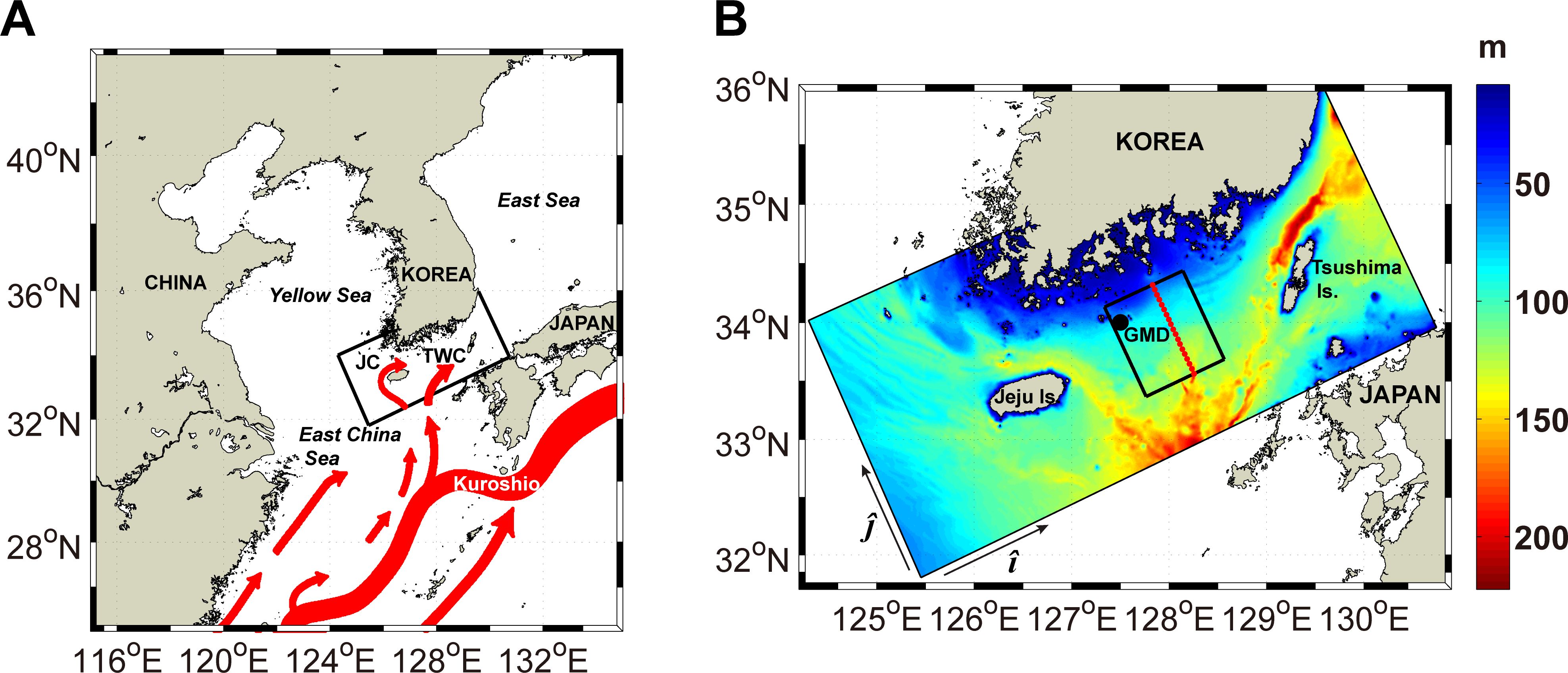
Figure 1. (A) Schematic surface ocean current system (Park et al., 2014) and model domain (black rectangle) including the Korea Strait (KS). (B) Modeling domain including the KS is outlined by the large black rectangle showing the bottom depth (colored shading). All analyses in this study were conducted within the small black rectangle, and all vertical cross-strait transects are conducted along the red dotted line. The black dot indicates the location of the automatic weather station at Geomun Island (GMD).

Son et al. (2010) examined the front and filaments that form between the KCW and TWCW using satellite sea surface temperature (SST) data and observed in-situ temperature and salinity profiles and currents in the frontal zone. They reconstructed the three-dimensional structure of the front with a meandering wavelength of 30−35 km using the retrogressive vector diagram method (RVDM) and revealed thermohaline interleaving intrusions across the front and the meandering of the front due to baroclinic instability. Similarly, Lee and Choi (2015) analyzed in-situ temperature and salinity datasets from a mooring in the KS in autumn and reported that the meandering of the thermohaline front between the KCW and TWCW was associated with the local sea level slope and vertical structure of the currents. Zhang et al. (2019) also conducted sensitivity experiments under uniform wind stress to investigate the mechanisms of front genesis and eddy formation in the summer Chukchi Sea, where a submesoscale eddy was detected by satellite. Down-front wind intensified the front and the accumulated mean available potential energy (MAPE), which was then converted to eddy available potential energy (EAPE). This EAPE was transferred to eddy kinetic energy, resulting in submesoscale eddy formation. Their study found that the total depth of the front, the vertical length scale of the front, was the key factor associated with eddy activity.

In this study, the development of the thermohaline front in the KS was confirmed by examining the time-varying horizontal surface temperature gradient from 2006 to 2012 using SST data from the Operational Sea Surface Temperature and Sea Ice Analysis (OSTIA) system operated by the Met Office (Donlon et al., 2012; Figure 2). In general, the horizontal temperature gradient exceeded 0.025°C km^-1 from September to October and maintained a strong gradient structure until February (Figure 2A). However, the temperature gradient weakened from March and persisted in this state until July. This indicates that KCW is formed by winter monsoon winds and cooling from autumn to winter, subsequently creating the thermohaline front with the relatively warmer TWCW. During this period, the front and geostrophic currents intensify in the KS due to the horizontal temperature gradient, which is either fully developed or in the process of developing by November (Figure 2). However, the horizontal temperature gradients in November of 2006 and 2009 differed from the other years, consistently weakening from mid-November (Figure 2B). These changes in the temperature gradient are indicative of variation in the ocean state, such as the current and density structures in the upper mixed layer.

Figure 2

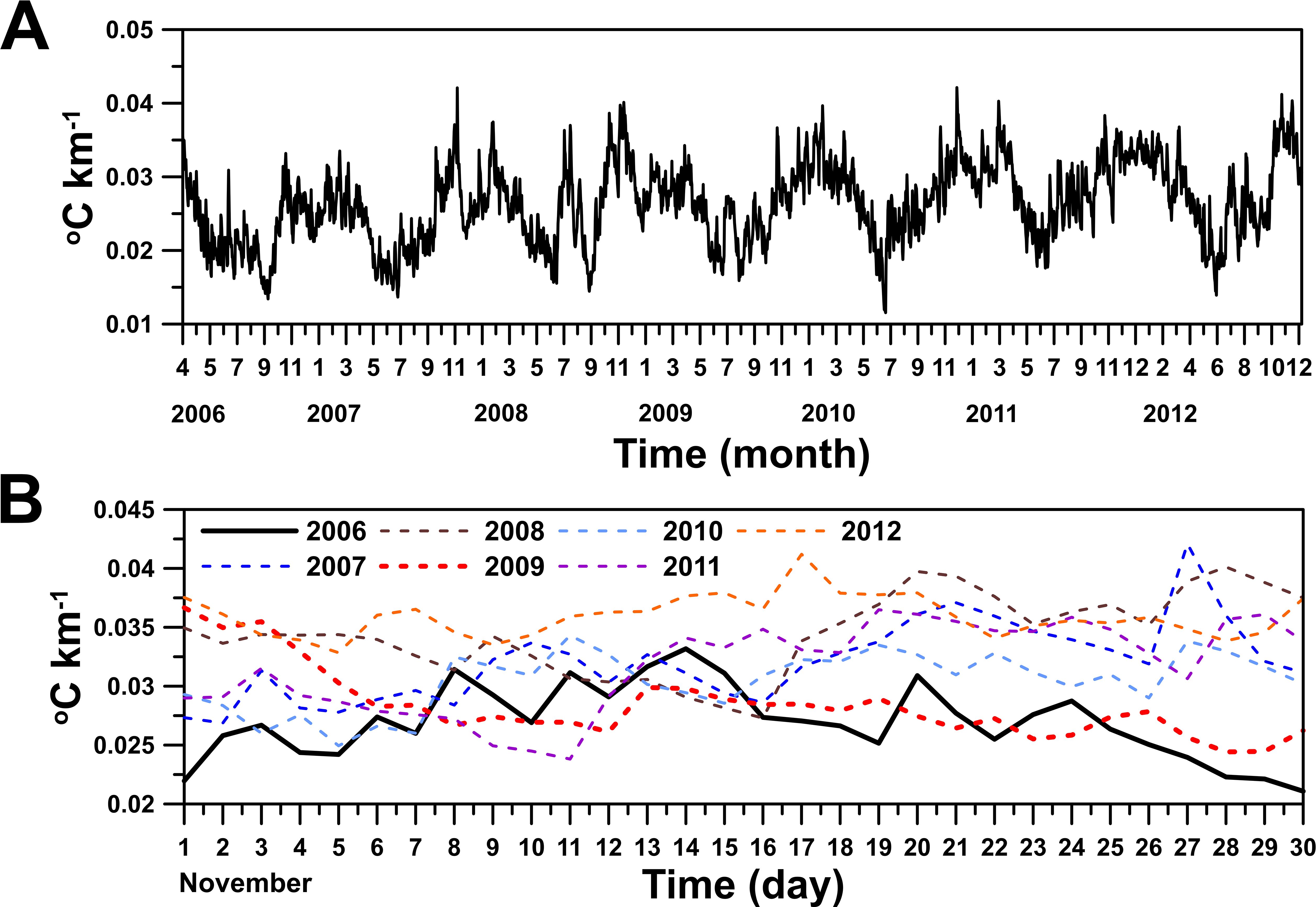
Figure 2. (A) Daily meridional surface temperature gradient within the black rectangle in (Figure 1A) from 2006 to 2012 and (B) daily meridional temperature gradient for November. The temperature gradients are calculated from Operational Sea Surface Temperature and Sea Ice Analysis (OSTIA) sea surface temperature (SST) data. The thick black, blue, red, dark brown, light blue, purple, and orange lines indicate the horizontal temperature gradient in November 2006, 2007, 2008, 2009, 2010, 2011, and 2012, respectively.

The development process of submesoscale features in the KS has not yet been simulated or analyzed. Therefore, this study aimed to understand the physical processes associated with variation in submesoscale features such as filaments and eddies during periods of high and low horizontal temperature gradients in the KS during autumn. In this study, mesoscale refers to a horizontal spatial scale larger than O (10 km), which is equal to or larger than the internal Rossby radius of deformation $L_R$ but smaller than 100 km. In contrast, submesoscale refers to a scale smaller than $L_R$, which is approximately 12–15 km in the KS during autumn (Lee and Choi, 2015). In this study, a three-dimensional ocean circulation model was used to simulate realistic thermohaline front and submesoscale features and to understand their response to changes in the wind over periods of 2–6 days. This time scale was selected because, in the KS, the wind direction changes every 2–6 days, and the front and submesoscale features respond to these changes. However, the response of the thermohaline front, the coastal jet, and the submesoscale features to wind variation over this time scale has not previously been reported.

The rest of this paper is structured as follows. First, the numerical model and simulations are described in Section 2. Section 3 then presents the results for changes in the submesoscale features and the thermohaline front due to up-front and down-front winds. Finally, Sections 4 and 5 present the discussion and conclusion, respectively.

2 Data and methods

2.1 Numerical model

In the present study, the Regional Ocean Modeling System (ROMS; Haidvogel et al., 2000; Shchepetkin and McWilliams, 2005) was used to simulate circulation in the KS from July to November 2006. The ROMS, which is a free-surface ocean model, uses the Boussinesq and hydrostatic approximations for the vertical momentum balance. A stretched terrain-following vertical coordinate and an orthogonal curvilinear horizontal coordinate are used. To reduce the calculation time, ROMS employs a split-explicit time-stepping scheme that calculates the barotropic and baroclinic modes separately. ROMS is a hydrostatic model and may not fully simulate the intrusion structures of temperature and salinity occurring during the baroclinic instability (Son et al., 2010). However, Mahadevan (2006) examined the role of nonhydrostatic effects on submesoscale processes at ocean fronts and found that the average vertical flux is similar in both hydrostatic and nonhydrostatic models. Additionally, it was reported that the submesoscale features remain robust at horizontal grid resolutions ranging from 1 to 0.25 km.

The model domain connects the East China Sea to the East Sea and includes Jeju and Tsushima Islands, and the KS (Figure 1B). The water depth is shallower than 200 m within the model domain. The nominal horizontal grid spacing of the model is approximately 1 km, and 41 vertical levels were used. To replicate heat exchange between the atmosphere and ocean, bulk flux formulae were used (Fairall et al., 1996). The horizontal viscosity was set to 2 m² s^-1 (Son, 2008), while Mellor and Yamada 2.5 closure (MY25) was used in the vertical mixing parameterization (Mellor and Yamada, 1982). Initial conditions and open boundary data, such as the daily mean temperature, salinity, velocity, and sea level were taken from a regional northwestern Pacific Ocean circulation model with a horizontal grid spacing of 10 km (Seo et al., 2014). A high-resolution model for the KS with a grid spacing of 1 km was nested within the regional northwestern Pacific Ocean model using a one-way nesting method. Tidal waves were propagated into the model domain across the four open boundaries and the harmonic constant of eight tidal constituents (M₂, S₂, N₂, K₂, K₁, O₁, P₁, and Q₁) were obtained from Nao99jb (Matsumoto et al., 2000). Surface atmospheric forcing data such as atmospheric temperature and pressure, relative humidity, and shortwave radiation were obtained from the European Centre for Medium-Range Weather Forecasts (ECMWF) reanalysis data. Bottom topography data were interpolated from local 30 s gridded bathymetric data (Seo, 2008) within the model grid.

The small black rectangle in Figure 1B indicates the study area, within which dynamic analysis of the submesoscale features was conducted using simulated daily mean data. In this area, the bathymetry was smoother than in the other regions of the KS. Due to this smoother bathymetry, this region was selected to minimize variation in the vertical velocity caused by the bathymetric effect.

2.2 Atmospheric data

Ekman transport plays an important role in the development of the thermohaline front (Thomas and Lee, 2005). This study examined the variability of the thermohaline front in response to wind variations, making it essential to verify the reanalysis wind data used as atmospheric forcing. Additionally, it was necessary to identify the cause of wind variation.

To validate the reanalysis wind data and confirm variations in the realistic wind pattern, hourly mean observations of the wind at Geomun Island (GMD), located in the middle of the model domain, were obtained from an automatic weather station maintained by the Korea Meteorological Administration (KMA). Daily average data were generated from the hourly mean wind observations. The daily wind data were then compared with the daily mean reanalysis winds.

To identify the cause of surface wind variations, the 300 hPa pressure surface height field from ERA5 reanalysis data, provided by the ECMWF (https://cds.climate.copernicus.eu), was used. The datasets had a spatial resolution of 25 km with 1-hour time intervals. Using the hourly 300 hPa pressure surface height field, temporal averages from November 11 to 14 and from November 22 to 26 were calculated. Subsequently, the variations in surface wind patterns were examined.

3 Results

3.1 Variability in the monsoon wind patterns

The wind generally blew toward the southeast from November 1 to 15, and then changed direction to the southwest starting on November 16 (Figure 3). The surface wind switched back to the southeast on November 28. These observed winds were compared with the reanalysis winds used as atmospheric forcing for the nested high-resolution model for the KS. The reanalysis winds from the ECMWF at Geomun Island and their spatial average over the entire model domain exhibited similar temporal wind variations to the observations (the red and blue vectors, respectively, in Figure 3).

Figure 3

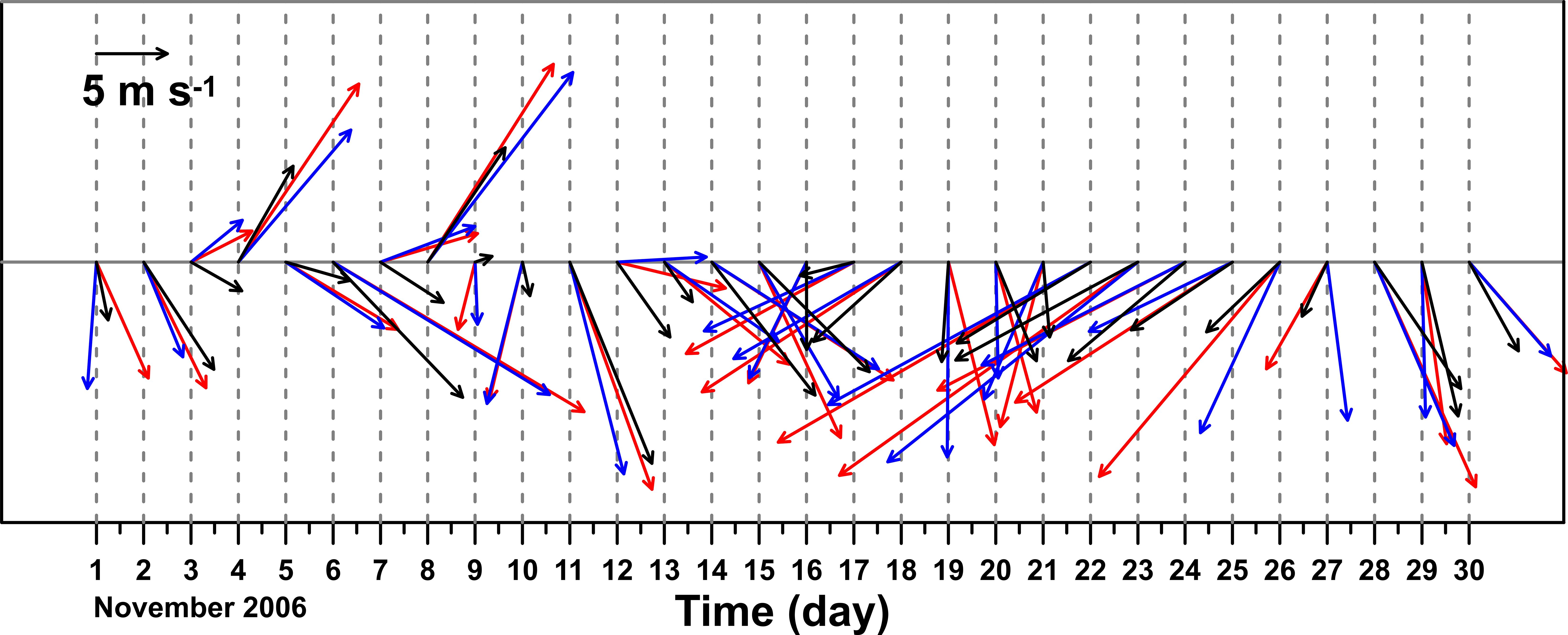
Figure 3. Daily mean wind vectors from November 1 to 30, 2006. The red vectors represent the winds from the European Centre for Medium-Range Weather Forecasts (ECMWF) model near Geomun Island. The blue vectors represent the spatially averaged ECMWF model winds within the small black solid rectangle in F (Figure 1B). The black vectors represent the winds observed at Geomun Island.

To determine the relationship between the surface winds and upper tropospheric circulation during northwesterly and northeasterly wind events, the spatial distribution of the 300 hPa pressure surface height and the surface winds were analyzed for November 14 and 23 (Figure 4). The jet stream migrates north and south in time, and it fluctuates due to baroclinic instability (O’ Sullivan and Dunkerton, 1995). The 300 hPa pressure surface height in the upper troposphere, which corresponded roughly to an altitude of around 10 km, was close to the level where winds are usually strongest (Figure 4). The contours of the 300 hPa pressure surface height converged over the KS on November 14. When the converging area of the jet stream, which was located in the western part of the trough in the 300 hPa pressure surface height, moved over the KS, the strong upper troposphere wind reached the bottom of the atmosphere, resulting in strong northwesterly winds at the ocean surface (Jhun and Lee, 2004). Strong northwesterly winds were observed at GMD and simulated in the ECMWF model over the KS on November 14 (Figures 3, 4C). When the convergence region of the jet stream in the upper troposphere moved farther eastward, the surface pressure pattern changed and northeasterly winds appeared at the surface (Figure 4D). Relatively strong northeasterly winds were observed at GMD and simulated in the ECMWF model over the KS on November 23 (Figures 3, 4D).

Figure 4

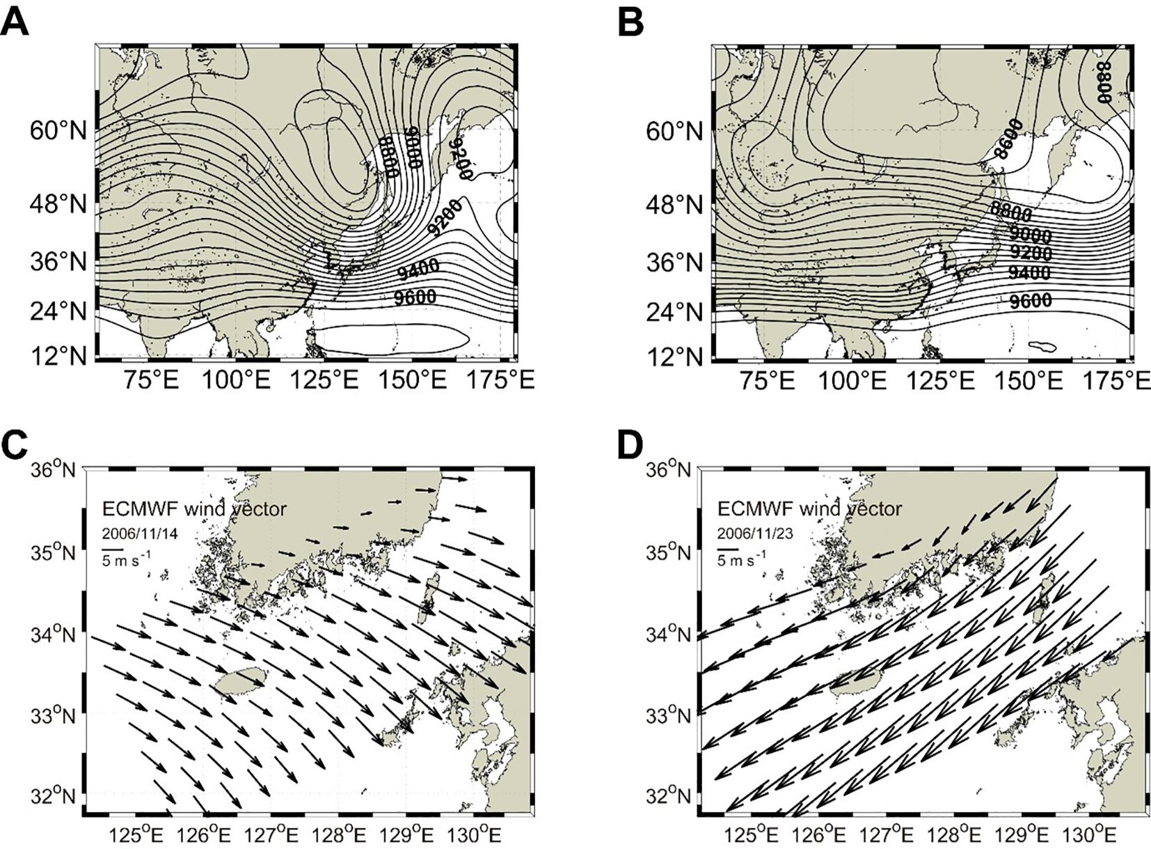
Figure 4. Temporal means of 300 hPa pressure surface height from (A) November 11 to 14 and (B) November 22 to 26, 2006, in the East Asia and Northwestern Pacific region (${60}^{°}\text{E to }{180}^{°}\text{E}$ and ${10}^{°}\text{N to }{70}^{°}\text{N}$; https://cds.climate.copernicus.eu). Daily mean surface wind vectors on November (C) 14 and (D) 23 from ECMWF reanalysis within the modeling domain.

3.2 Frontal and filamentary structures in autumn

To verify the position and meandering pattern of the thermal front, snapshots of the satellite-derived SST and model-simulated temperature at a depth of 2 m were compared (Figure 5). The satellite SST data were provided by the Korea Ocean Satellite Center at the Korea Institute of Ocean Science & Technology (KIOST), which produces SST products from advanced very high-resolution radiometer (AVHRR) data. The thermal front formed between Jeju and Tsushima Islands in both the satellite SST and model-simulated temperature data. There was a strong temperature gradient (0.72°C km^-1) between the isothermal lines of 18°C and 21°C. The 19, 20, and 21°C isotherms formed an eastward finger-shaped intrusion at 129°E, 34.5°N to the west of Tsushima Island (Figures 5A, B). The temperature gradient of the thermal front increased to 1.12°C km^-1 on November 14. Although the numerical model did not produce filaments that were in the exact locations observed in the satellite-derived SST images, the model-simulated temperature distribution exhibited similar features to the observed distribution, including submesoscale perturbations and horizontal intrusions (Figures 5C, D). A free-running model without data assimilation cannot precisely replicate frontal and submesoscale feature patterns due to the non-deterministic nature of the instability in the surface ocean. During northwesterly wind events, both the satellite-derived SST images and the model-simulated temperature distribution had submesoscale perturbations, such as filaments and eddies, along the thermal front.

Figure 5

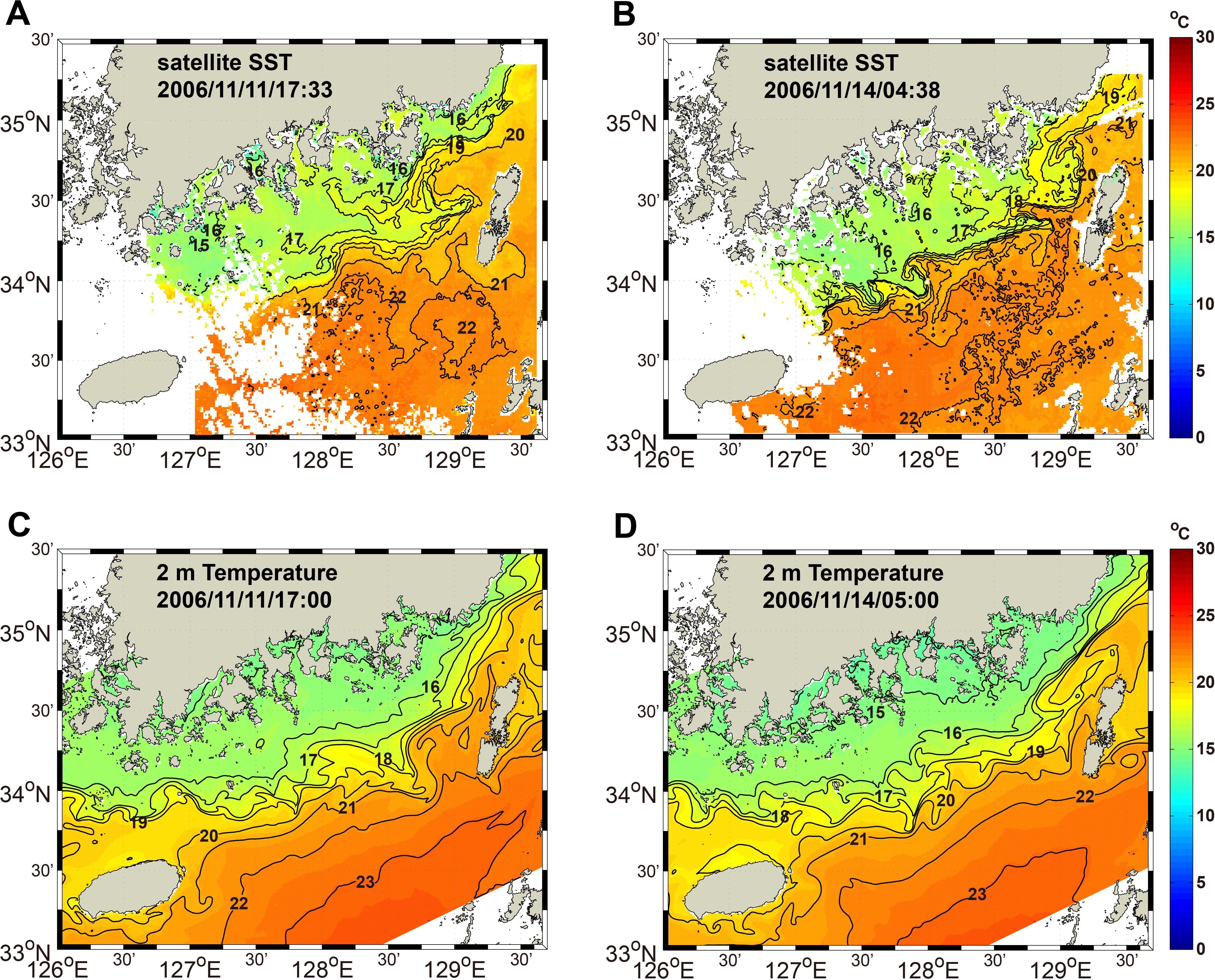
Figure 5. Horizontal distribution of the SST from satellite measurements on (A) November 11 at 17:33 and (B) November 14 at 04:38 GMT. The white area in (A, B) indicates cloud cover. Horizontal distribution of the hourly mean temperature at a depth of 2 m from the numerical model on (C) November 11 at 17:00 and (D) 14 at 05:00 GMT.

3.3 Horizontal distribution of the currents and density

To examine the variation in the frontal structure in response to changes in the wind, the horizontal distribution of the currents and isopycnals on November 14 and 23 were analyzed (Figures 6A, B). With northwesterly winds on November 14, the relatively light TWCW (${\sigma }_t\le 24$) flowed northeastward in the mid-KS, while the relatively dense KCW (${\sigma }_t\ge 25$) moved eastward, encroaching on the TWCW (Figure 6A). The northward currents along the east and west coasts of Jeju Island converged northeast of Jeju Island and then flowed eastward. The converging TWCW encountered the southeastward-flowing KCW, forming a jet to the northeast of Jeju Island. The flow then continued eastward along the isobaths. Offshore surface currents flowed along the front, while surface currents were relatively weak in the shallow coastal region north of the front. Significant meandering of the front and surface currents occurred between Jeju and Tsushima Islands. The density gradient ($\left|\sqrt{{(\partial \rho /\partial x)}^2+{(\partial \rho /\partial y)}^2}\right|$) was more pronounced along the northern boundary of the TWC (Figure 6C). The Rossby number (Ro = ${\zeta }_z/f$), where ${\zeta }_z$ and $f$ represent the relatively vorticity and Coriolis parameter respectively, was relatively high along the front, where submesoscale features developed (Figure 6E).

Figure 6

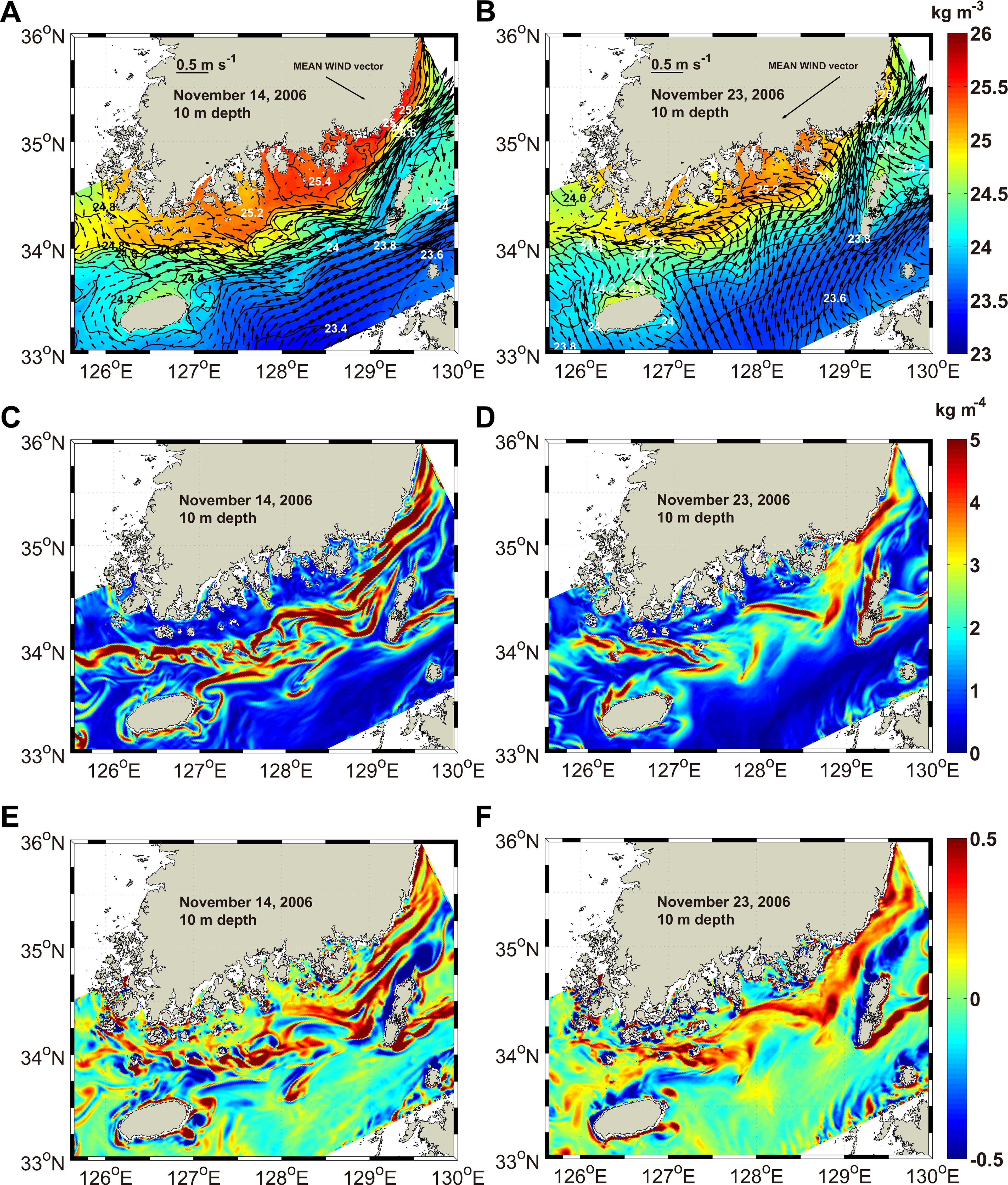
Figure 6. Horizontal distribution of (A, B) daily mean density field at a depth of 10 m (σ_t, contours and colors) with current vectors, (C, D) horizontal density gradient, (E, F) the Rossby number ($Ro={\zeta }_z/f)$ on (A, C, E) November 14 and (B, D, F) November 23, 2006. The density gradient unit is $1\times {10}^{-5}$ kg m^-4.

When the wind switched to northeasterly, the direction of the surface current rotated counterclockwise, flowing northward with surface currents crossing over the front (Figure 6B). This change in the surface current caused the TWCW to move over the KCW. Coastal currents flowed westward along the south coast of Korea in the shallow region. The density gradient was reduced along the front, and the meandering of the front became significantly weaker (Figure 6D). Ro remained high near the coastal region. However, it was significantly lower between Jeju and Tsushima Islands compared to November 14 (Figure 6F). On November 23, the horizontal distribution of Ro at a depth of 10 m showed a reduction in submesoscale features such as eddies and filaments.

3.4 Vertical sections of the background field

Vertical sections of currents and density and the sea surface height (SSH) distribution across the front on November 14 and 23 were examined with the aim of determining the relationship between the vertical circulation, horizontal position of the front, and along-strait current (Figure 7). The vertical sections were positioned as shown by the red dotted line in Figure 1B. The sticks in the bottom panels of Figure 7 represent the combined current vectors for the cross-strait (v) and vertical velocities (w). To clearly show the cross-strait vertical circulation, w has been amplified 10⁵ times in Figure 7.

Figure 7

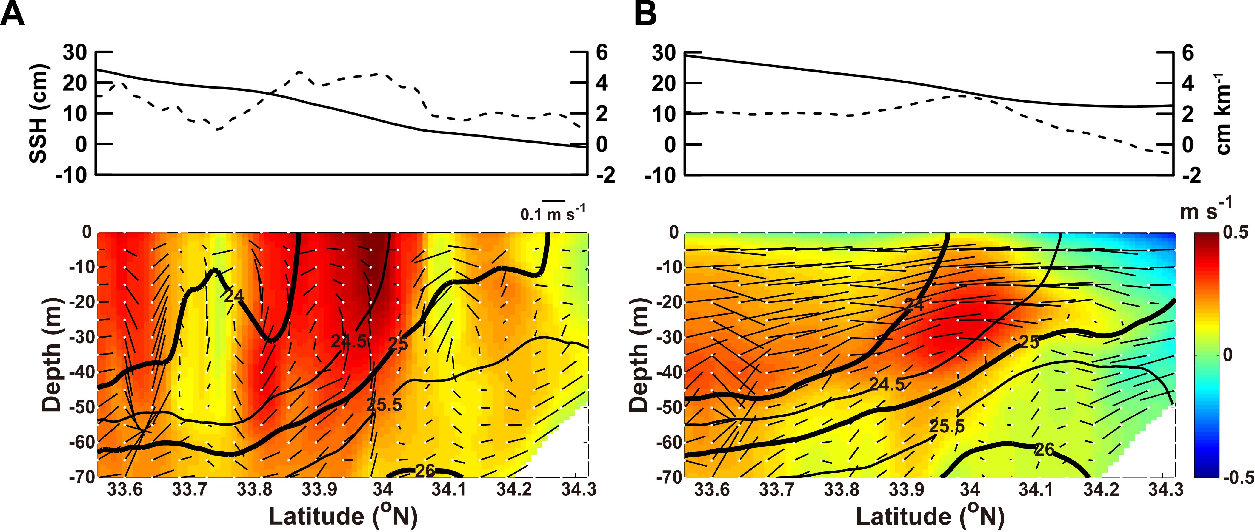
Figure 7. Cross-strait section of the sea surface height (SSH) (solid line), SSH gradient (dotted line), density (σ_t, line contours), along-strait velocity u (color contours), and combined cross-strait current vector ($v\widehat{j}+w\widehat{k}$) of cross-strait (v) and vertical (w) velocities on (A) November 14 and (B) November 23 across the KS [along the red dotted line in (Figure 1B)]. Red and blue shading of u represents eastward and westward flow, respectively. The contour interval of σ_t is 0.5. In the lower panels, the thick black lines represent the isopycnals σ_t = 24 and σ_t = 25. The SSH gradient unit is 1 $\times {10}^{-6}$ cm km^-1. To illustrate the vertical circulation pattern, the value of w is magnified by a factor of ${10}^5$.

With northwesterly winds, the cross-strait SSH gradient ($\partial \eta /\partial y$) was relatively high, while the along-strait velocity (u) was strong along the front in the upper 60 m near 33.6°N and from 33.8°N to 34.07°N, where a strong thermal front with vertically steep isopycnals was generated due to the merging of the TWCW and KCW (Figures 5, 7A). The maximum velocity of u was about 0.54 m s^-1 at the surface. Meridional overturning flows were active over the entire area, and these secondary circulations resulted in submesoscale upwelling and downwelling cells (Figure 7A). The horizontal length scale of these ageostrophic secondary circulations was approximately 9 km.

With the arrival of northeasterly winds on November 23, the sea level rose about 4.8 cm offshore and about 13.6 cm near the coast, resulting in a smaller SSH gradient than on November 14 (Figure 7B). Furthermore, submesoscale perturbations in the SSH gradient shorter than 10 km disappeared on November 23. Although the along-strait current (u) in the subsurface layer between depths of 10 and 50 m was maintained, the surface current speed decreased significantly. The cross-strait current (v) was positive, and the surface water moved toward the coast in the upper depths of 40 m. The surface water downwelled north of 34.2°N. This downwelling process, induced by the northeasterly wind, flattened the isopycnals. While the TWC flowed to the northeast (i.e., out of the page in Figure 7B) in the mid-KS, the along-strait current flowed to the west (i.e., into the page in Figure 7B) in the shallow coastal region north of 34.2°N.

The width of the simulated jet (L_h; horizontal length scale) was approximately 31 km, and the L_R was about 10.4 km in the simulated field for November 2006 (Figure 7). In the KS, the observed length scale of the subsurface (40 m) front was about 30 km, while the L_R ranged from 12 to 15 km estimated from the observed hydrography and current data in October 2009 (Lee and Choi, 2015). This indicates that the simulated along-strait current profile, horizontal length scale of the jet, and L_R were consistent with those reported by Lee and Choi (2015). A two-dimensional (vertical and seaward) model was used by Ikeda (1985) to understand the effects of along-shore wind on a front, with the results applied to the Labrador shelf front. The numerical modeling results indicated that a shoreward thin surface Ekman flow arising from wind blowing along the coast maintains the front, while seaward surface flow relaxes the front over the Labrador continental shelf slope. Similarly, in the present study, the direction of the along-strait wind affected the direction of the thin surface Ekman flow and the intensity of the front (i.e., the steepness of the isopycnals) in the KS.

The structures of the currents, pressure gradient, Coriolis force, and vertical friction terms in the cross-strait momentum equation along the red dotted line shown in Figure 1B were compared between November 14 and 23 to determine which forces were most influential (Figure 8). The advection and horizontal friction terms were relatively small and are not shown here. On November 14, when northwesterly winds were present, the pressure gradient and Coriolis terms around the core of the along-strait jet were larger than $20\times {10}^{-6}$ m s^-2 and smaller than $-20\times {10}^{-6}$ m s^-2, respectively (Figures 8A, C), indicating that the along-strait jet was primarily in geostrophic balance. The frictional force of the upwelling-favorable wind influenced the surface current from the surface to a depth of 10 m. The frictional term in the upper 10 m layer was as large as $-5\times {10}^{-6}$ m s^-2 (Figure 8E). In contrast, on November 23, under the influence of northeasterly winds, the pressure gradient and Coriolis forces were significantly weaker (Figures 8B, D). However, the frictional term was as large as $-20\times {10}^{-6}$ m s^-2 in the near-surface layer and larger than $5\times {10}^{-6}$ m s^-2 in the subsurface layer (25–40 m). The strong frictional force in the near-surface layer promoted cross-frontal advection from offshore to the coast, driving surface Ekman transport toward the coast.

Figure 8

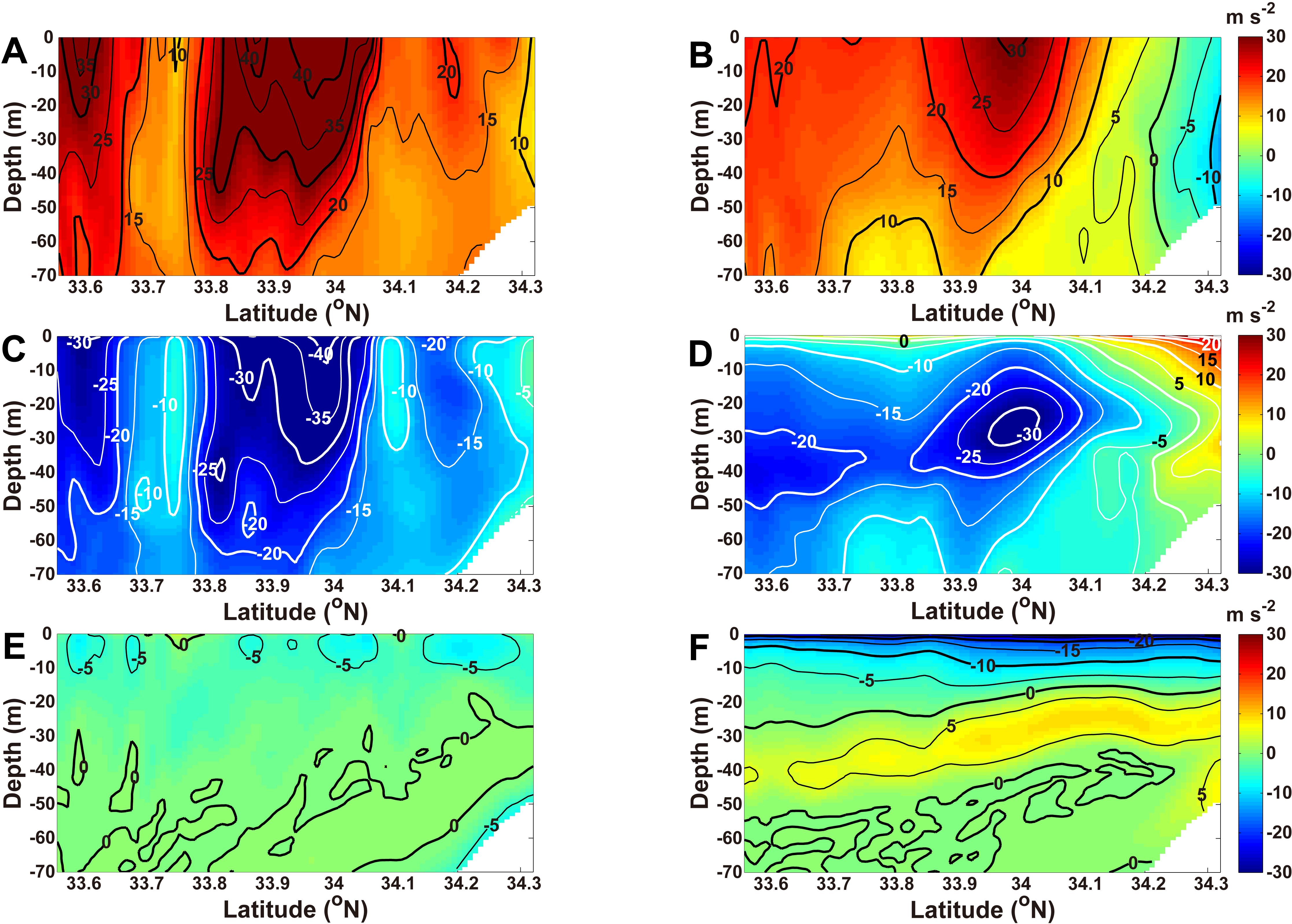
Figure 8. Vertical structures of the dominant terms in the cross-strait direction momentum balance on November 14 (left panels) and November 23 (right panels) along the red dotted line in (Figure 1B): (A, B) pressure gradient, (C, D) Coriolis (-fu), and (E, F) frictional forces. The contour interval is $5\times {10}^{-6}$ m s^-2.

3.5 Growth and decay of the submesoscale features

To quantify the wavelength of the submesoscale features and meanders during northwesterly wind events, spectral analysis was conducted on the simulated density and temperature data along the along-strait transects in the study area (Figure 9). Under the influence of the northwesterly wind from November 10 to 14, the ensemble mean power spectral density (PSD) function for the density field increased at a submesoscale wavelength of approximately 10 km on November 10, and these peaks persisted until November 17 (Figure 9A). These features were more pronounced in the ensemble mean PSD function for the temperature field (Figure 9B). In the temperature PSD function, spectral energy emerged at wavelengths of 6–10 km from November 9 to 17. The amplitudes of the submesoscale features with wavelengths less than 10 km diminished after November 17. By November 25, spectral energy for the submesoscale wavelengths disappeared in both PSD distributions. The enhancement and decay of the mesoscale features with wavelengths of 30–80 km occurred simultaneously with those of the submesoscale features. The northwesterly wind, which acted as a down-front wind, was the primary driving force behind the development of the meandering and filamentary structures in the KS.

Figure 9

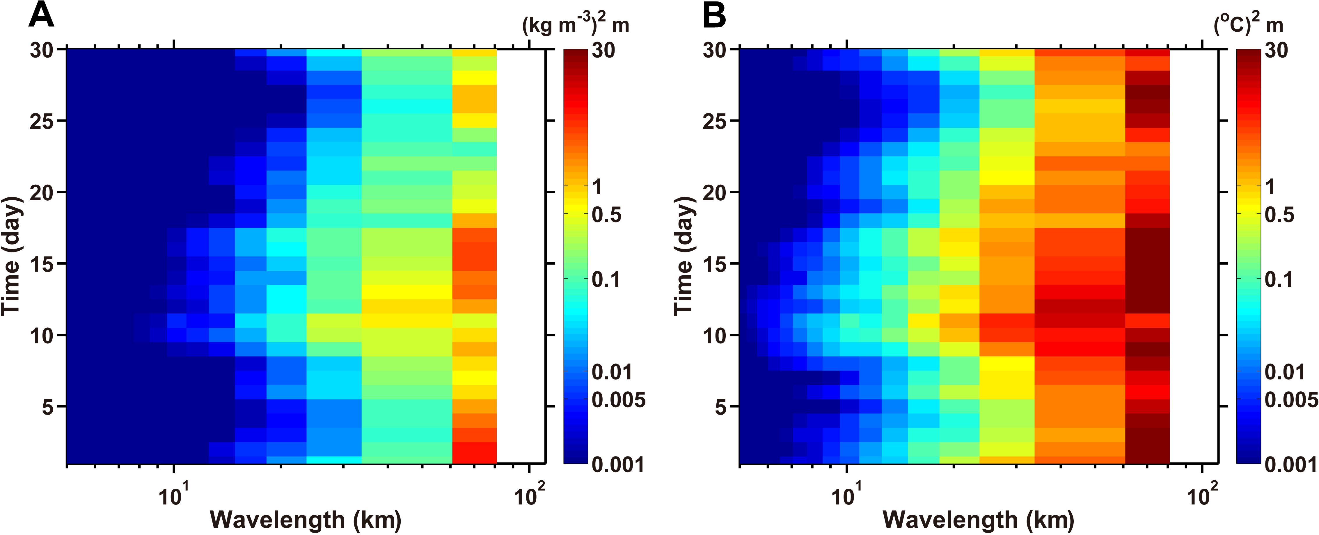
Figure 9. Time-series of the ensemble mean power spectral density (PSD) for (A) density and (B) temperature variations along the strait at a depth of 10 m in November. The density and temperature data are obtained from all along-strait transects in the small black rectangle in (Figure 1B). The ensemble mean PSD is calculated for each transect and then averaged for each wavelength bin. The along-strait transect is 83 km long. The color bar is on a log scale.

The growth and decay of submesoscale features were significantly related to the stability of the water column (Yang et al., 2021b). When down-front (up-front) wind blew, the buoyancy frequency ($N^2$) decreased (increased) and vertical circulation developed (weakened) in the upper mixed layer. Submesoscale features, such as filaments, were prominent in regions with strong vertical circulation (Rosso et al., 2014).

To examine the stability of the water column in relation to changes in the wind, the time-varying wind stress, buoyancy frequency, available potential energy (APE), and EAPE were compared (Figure 10). The buoyancy frequency square ($N^2$) was calculated using Equation 1:

Figure 10

Figure 10. (A) Time series of along-strait wind stress (${\tau }_x$, solid line) and time-integrated wind stress (dotted line) in November 2006. (B) Time series of the spatially averaged available potential energy (APE, solid line), eddy available potential energy (EAPE, dotted line) and buoyancy frequency ($N^2$, dashed line). The unit for $N^2$ is $1\times {10}^{-4}$ s^-2. The APE, EAPE, and $N^2$ in (B) were calculated from the small black rectangle in (Figure 1B).

$\begin{array}{ll}{N}^2=-\frac{g}{{\rho }_0}\frac{d\rho }{dz}& (1)\end{array}$

where $g$ is the acceleration due to gravity (9.81 m s^-2), ${\rho }_0$ is the reference density (1025 kg m^-3), and $\rho$ is the simulated potential density.

The APE was defined using Equation 2 (Gill, 1982):

$\begin{array}{ll}APE=\frac{g^2{\rho }_d^2}{2{\rho }_0{N}_d^2}& (2)\end{array}$

where ${\rho }_d$ is the deviation from the spatial and temporal mean density profile, which was calculated as follows:

${\rho }_d(x, y, z, t)=\rho (x, y, z, t)-\tilde{\rho }(z)$, where $\tilde{\rho }(z)$ is the horizontal and temporal mean vertical profile of $\rho (x, y, z, t).$ $N_d^2$ is the buoyancy frequency square with the density deviation (Kang and Curchitser, 2015) and was calculated using Equation 3:

$\begin{array}{ll}{N}_d^2=-\frac{g}{{\rho }_0}\frac{d{\rho }_d}{dz}& (3)\end{array}$

To calculate the EAPE, the perturbation density (${\rho }_d^{\prime }$) was obtained from the equation ${\rho }_d^{\prime }={\rho }_d-\overline{{\rho }_d}$, where $\overline{{\rho }_d}$ is the temporal mean of ${\rho }_d$ (Kang and Curchitser, 2015). The EAPE was calculated using Equation 4:

$\begin{array}{ll}EAPE=\frac{g^2\rho {\prime }_d^2}{2{\rho }_0{N}_d^2}& (4)\end{array}$

The APE, EAPE, and $N^2$ were spatially averaged over the study area.

The along-strait wind stress (${\tau }_x$) was spatially averaged over both the entire study area and the entire model domain. It was calculated using Equation 5:

$\begin{array}{ll}{\tau }_x={\rho }_a{C}_{D}W{W}_x& (5)\end{array}$

where ${\rho }_a$ is the density of air (1.2 kg m^-3), $W$ is the wind speed, and $W_x$ is the along-strait wind velocity. $C_D$ is the air drag coefficient, which is modified by the wind speed based on Large and Pond (1981) and Trenberth et al. (1990) as follows (Equation 6):

$\begin{array}{ll}{C}_D=\{\begin{array}{l}0.00218 W\le 1 m s^{-1}\\ 0.001 (0.62+1.56W^{-1}) 1 m s^{-1}<W\le 3 m s^{-1}\\ 0.00114 3 m s^{-1}<W\le 10 m s^{-1}\\ 0.001 (0.49+0.065W) W>10 m s^{-1}\end{array}& (6)\end{array}$

Along-strait wind blowing toward the northeast induced upwelling and intensified the front because it traveled in the direction of the frontal jet. With the along-strait wind blowing toward the northeast from November 1 to 9, the time-integrated value of ${\tau }_x$ continued to increase until November 9 (Figure 10A). The variation in ${\tau }_x$ over time within the study area was also consistent with that over the model domain. From November 9 to 11, ${\tau }_x$ was negative, while it was positive until November 14. The time-integrated ${\tau }_x$ increased toward a positive value until November 15 (Figure 10A). Both the APE and EAPE gradually increased starting from November 9 and then abruptly increased from November 13 to 15 (Figure 10B). During this period, the time-integrated value of ${\tau }_x$ also increased, reaching a peak on November 14. During this peak, the meridional gradient of the SST was also at its highest point (Figure 2B).

Temporal variation in the APE, EAPE, and $N^2$ responded sensitively to the time-integrated value of ${\tau }_x$, with the same signs for the APE and EAPE and the opposite signs for the $N^2$ from November 13 to 15. This indicates that the strong westerly winds (i.e., along-jet or down-front winds) actively generated spatial differences and temporal perturbations in the water density and effectively reduced vertical stratification within the study area. The higher mean kinetic energy supplied energy to the APE, while the higher APE supplied energy to the EAPE (Figure 6A, C). The increase in the EAPE, coupled with the decrease in $N^2$, produced favorable conditions for flow instability, which facilitated the development of mesoscale current meandering, submesoscale intrusions, and filaments across the front during this period (Figures 4, 5).

The water column stabilized from 16 to 28 November because the ${\tau }_x$ became negative due to the easterly wind (Figure 10). After November 16, the time-integrated value of ${\tau }_x$ decreased and became negative on November 21 (Figure 10A). Following November 16, both the APE and EAPE significantly decreased while $N^2$ increased again (Figure 10B). The easterly wind acted as an up-front wind with the weakening of the front strength and along-front current and the reduction of the submesoscale features in the KS.

3.6 Variation in the submesoscale features and the secondary circulation

In the previous section, the growth and decay of the APE and EAPE were found to be related to the changes in the wind. In this section, the effect of ageostrophic secondary circulation, which is also influenced by the wind, on the stability of the water column is examined. The ageostrophic horizontal current velocity ${\overrightarrow{V_a}}_{ }=u_a\widehat{\mathit{i}}$+ $v_a\widehat{\mathit{j}}$ was calculated using Equation 7 (Wenegrat and McPhaden, 2016):

$\begin{array}{ll} \overrightarrow{V_a} = \overrightarrow{V}-\overrightarrow{V_g} & (7)\end{array}$

where $\overrightarrow{V}$ is the simulated total horizontal current and $\overrightarrow{V_g}$ is the geostrophic horizontal current, which is calculated using the simulated sea level and density. From the momentum balance analysis, the pressure gradient and Coriolis force terms were in primary balance on November 14. However, the vertical friction term was prominent in the upper layer (Figure 8). $\overrightarrow{V_a}$ is mainly induced by vertical frictional force and promotes the development of ageostrophic secondary circulation (McWilliams, 2017).

On November 14, the ${\overrightarrow{V_a}}_{ }$ at a depth of 10 m flowed southwestward across the thermohaline front with an approximately rightward normal direction to the direction of the wind (Figures 4C, 11A). The relatively denser water (${\sigma }_t=24.8$) intruded to the southeast toward the relatively lighter water at 127.63°E, 33.95°N and 127.94°E, 34.1°N where the EAPE was relatively high (Figure 11C). The daily mean vertical velocity (w) had an upward and downward maximum of $6.3\times {10}^{-4}$ m s^-1 ($54.38$ m d^-1) and $-9.7\times {10}^{-4}$ m s^-1 ($-83.85$ m d^-1) at a depth of 10 m, respectively (Figure 11E). Speckled (i.e., multipole) patterns in w were produced by the divergence of ${\overrightarrow{V_a}}_{ }$ (Figures 11E, G). In the distribution of ${\sigma }_t$, filamentary features were also generated by submesoscale upwelling and downwelling. It is important to emphasize that the southeastward expansion of the two isopycnal lines at ${\sigma }_t$= 24.6 and 24.8 was not induced by the horizontal velocity jet. Instead, this expansion was generated by the active vertical density flux, which was driven by the upward and downward vertical velocities and vertical mixing.

Figure 11

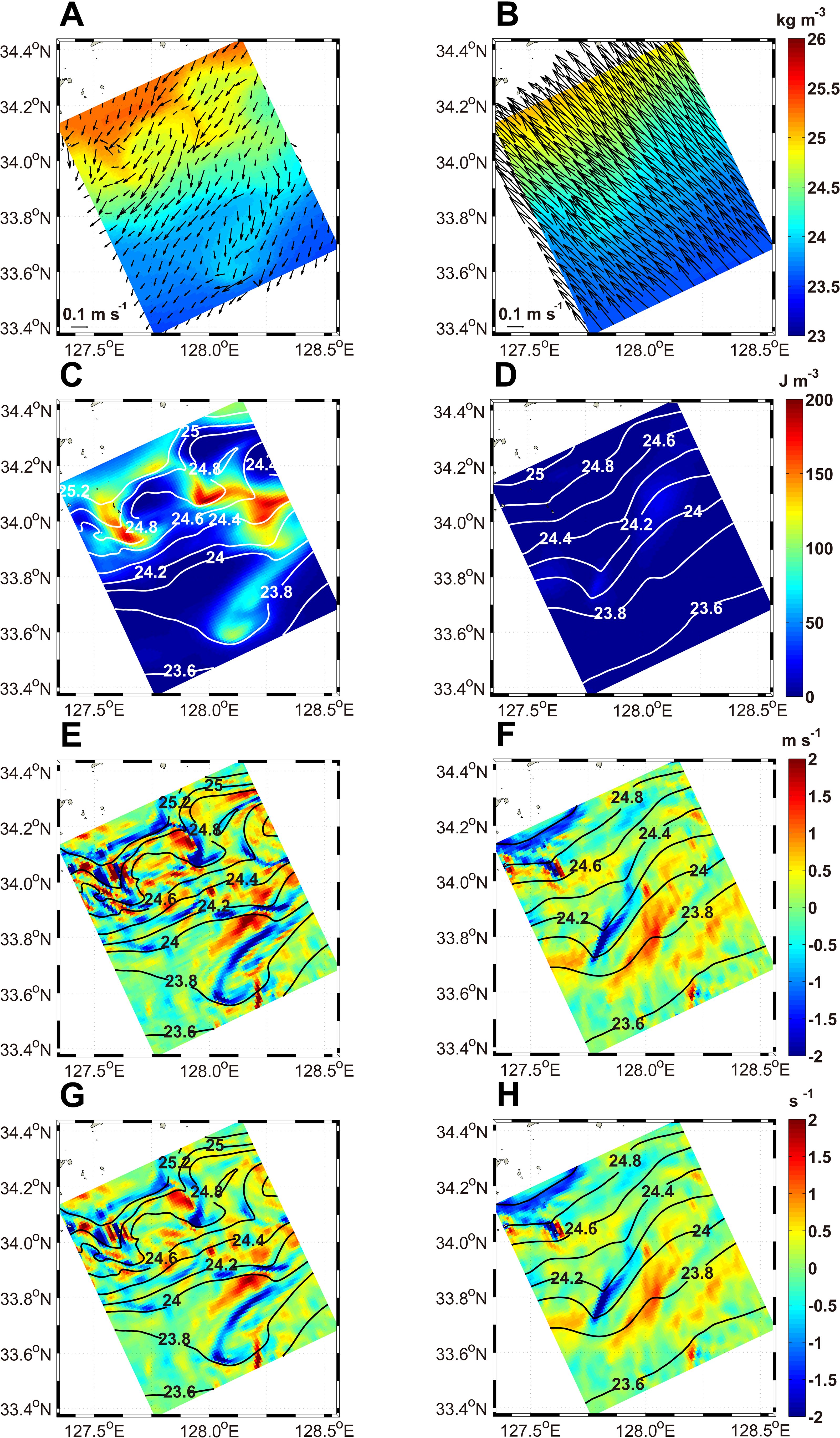
Figure 11. Horizontal distribution of the (A, B) ageostrophic currents (indicated by the vectors) and σ_t (colored shading), (C, D) EAPE, (E, F) simulated vertical velocity w, (G, H) divergence of ageostrophic currents at a depth of 10 m in the small black rectangle in (Figure 1B). The horizontal distributions in the left and right panels represent the simulation results for November 14 and 23, respectively. The contours in each panel represent σ_t. The unit for the divergence of the ageostrophic currents is $1\times {10}^{-5}{\text{ s}}^{-1}$. To compare the pattern in the ageostrophic current divergence with that of the vertical velocity (w), the values for w have been increased by a factor of ${10}^4$ in panels (E, F).

On November 23, ${\overrightarrow{V_a}}_{ }$ headed toward the northwest across the thermohaline front, with a rightward normal direction to the wind direction (Figure 11B). Over the entire domain, ${\sigma }_t$ was lower than on November 14 (Figure 11B), indicating that the water column became more stable. At around the onset of the up-front wind events, the filamentary features disappeared, and the isopycnals became smooth. During the up-front wind events, the EAPE decreased significantly to less than 40 J m^-2 and the speckled pattern in w was also reduced. The northwestward $\overrightarrow{V_a}$ was nearly uniform, while w and the divergence of ${\overrightarrow{V_a}}_{ }$ were relatively low (Figures 11D, F, H).

To assess the variation in the stability due to the ageostrophic secondary flow, the meridional sections of the ageostrophic secondary flow ($v_a \widehat{\mathit{j}}+w \widehat{\mathit{k}}$), the along-strait geostrophic current $u_g$, ${\sigma }_t$, the divergence of $\overrightarrow{V_a}$, $N^2$, and the EAPE were examined along the red dotted line shown in Figure 1B (Figure 12). The surface coastal jet ($u_g$) in geostrophic balance was strong from 33.77°N to 34.07°N, with a meridional width of approximately 30 km and a maximum speed of 0.56 m s^-1 at the surface of 33.88°N on November 14 (Figure 12A). Near the lateral boundaries of the coastal jet (33.72–33.82°N and 34.1–34.2°N), ageostrophic secondary circulations developed in the cross-strait section (Figure 12A). The divergence of $\overrightarrow{V_a}$ induced vertical motions (acting as a pump), resulting in the formation of multiple secondary clockwise circulation cells when viewed in a down-front direction (Figure 12C). The isopycnals ${\sigma }_t=24$ and ${\sigma }_t=25$ rose to a depth of 12 m at both lateral boundaries of the along-strait jet (Figure 12C). This indicates that down-front winds induced the ageostrophic secondary circulation, which subsequently strengthened the front and along-strait current (Thomas and Lee, 2005). In addition, at both lateral boundaries of jet, the stability of the water column was weakened and the EAPE increased (Figures 12E, G).

Figure 12

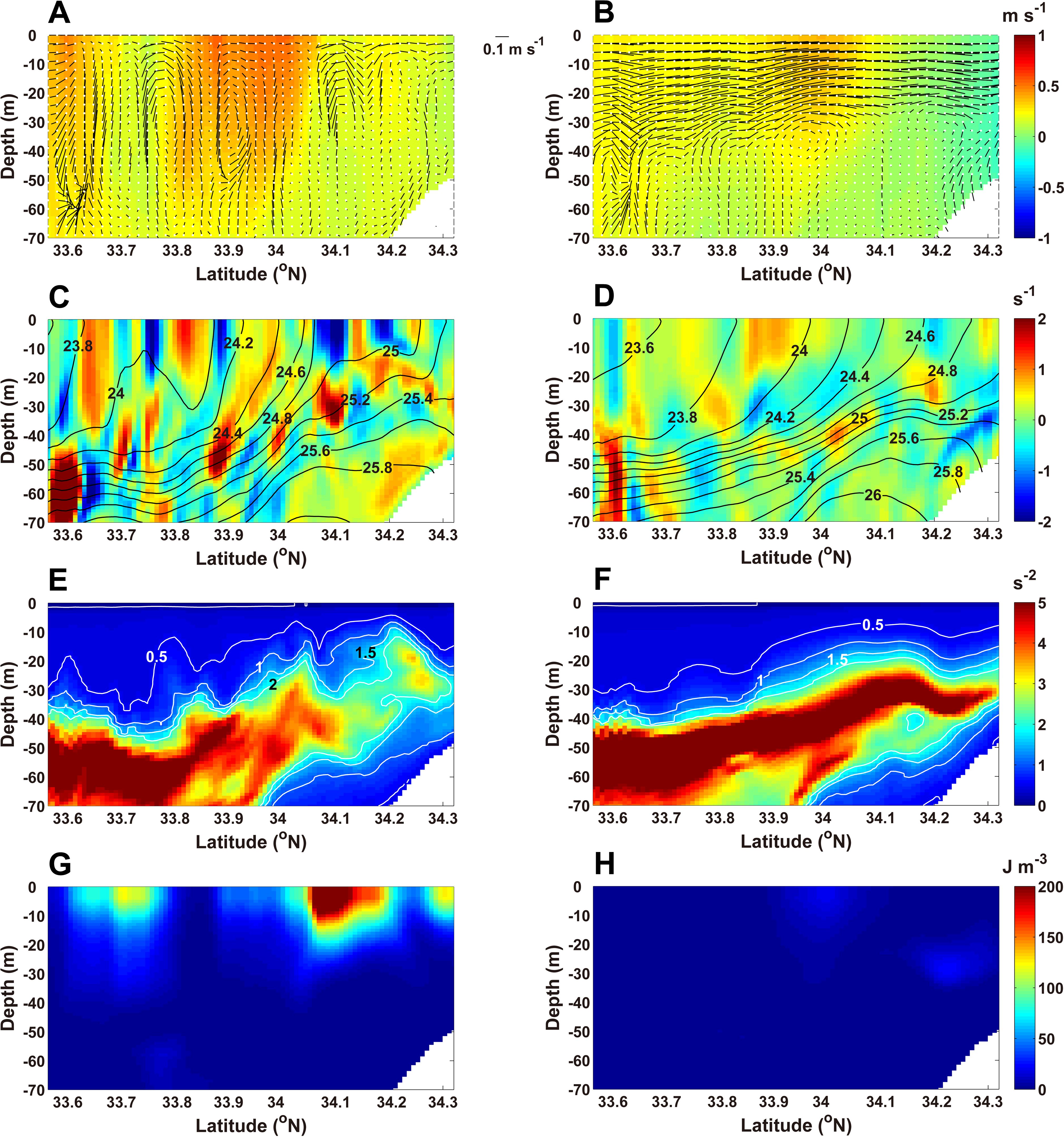
Figure 12. Vertical section of the (A, B) along-strait geostrophic velocity ($u_g$, colored shading) and combined current vectors ($v_a\widehat{j}+w\widehat{k}$) for the cross-strait ageostrophic current and vertical velocity, (C, D) divergence of the horizontal ageostrophic currents (colored shading) and σ_t (contours, kg m^-3), (E, F) buoyancy frequency square, and (G, H) EAPE along the red dotted line in (Figure 1B). The vertical sections in the left and right panels are the results for November 14 and 23, respectively. The units for the divergence of the horizontal ageostrophic currents and buoyancy frequency are $1\times {10}^{-5} {\text{s}}^{-1}$ and $1\times {10}^{-4}{\text{ s}}^{-2}$, respectively. To illustrate the vertical circulation pattern, w is amplified by a factor of ${10}^5$.

With the up-front winds on November 23, the ageostrophic secondary flow toward the coast became dominant from the surface to a depth of 30 m, forming a single counterclockwise circulation in the meridional section when viewed in the down-front direction (Figure 12B). The vertical motions diminished in the mid-strait, and the divergence and convergence of $\overrightarrow{V_a}$ significantly weakened (Figures 12B, D). Although the along-strait jet of $u_g$ was still present, it was much weaker than on November 14 (Figure 12B). The stratification increased from 33.9°N to 34.3°N over the northern bottom slope (Figure 12F), indicating that the water column became significantly more stable. The EAPE weakened significantly due to the enhanced stability in the water column (Figure 12H).

3.7 Divergence in $V_a$ and generalized Ekman pumping

On November 14, $\overrightarrow{V_a}$ was not spatially uniform (Figure 11A). This led to a strong horizontal divergence, resulting in vertical mixing (Figures 11E, G). While the northwesterly winds were relatively uniform (Figure 4C), the wind stress curl and Ekman pumping were relatively small. The loose spatial correlation between the northwesterly winds and $\overrightarrow{V_a}$ fields indicates that the influence of the wind on the ageostrophic flow at a depth of 10 m was weak. This depth was likely within the surface Ekman layer during late autumn. In the presence of down-front winds along the frontal zone, the horizontal density gradient across the front and the vertical shear of the geostrophic currents were enhanced due to the thermal wind balance (Figure 6C). The horizontal geostrophic flow cannot generate vertical velocity and mixing because it is nondivergent, $\nabla ·\overrightarrow{V_g}=0$. However, on November 14, vertical velocity was prominent within the study area (Figures 7A, 11E, 12A). These vertical velocities were related to the horizontal ageostrophic flow. Because divergent ageostrophic currents are part of the total current, the horizontal divergence of the total current ($\nabla ·\overrightarrow{V}$) induced vertical velocity.

To understand the formation of submesoscale features in the coastal frontal region, it is important to consider the impact of the vertical mixing of momentum due to surface layer turbulence, which is as important as the pressure gradient and Coriolis forces. When the Coriolis force, pressure gradient, and vertical friction terms are balanced in the horizontal momentum equation, this momentum balance can be expressed as shown in Equation 8A (Gula et al., 2014; Wenegrat and McPhaden, 2016; Xu et al., 2022):

$\begin{array}{ll}f\widehat{\mathit{k}}\times \overrightarrow{V}= -\frac{1}{{\rho }_0}{\nabla }_{h}P + {\nabla }_z(A_z {\nabla }_z\overrightarrow{V} ) & \text{(8A)}\end{array}$

$\begin{array}{ll} 0= -\frac{1}{\rho }{\nabla }_{z}P-g & \text{(8B)}\end{array}$

where $\overrightarrow{V}= \overrightarrow{V_g}$ + $\overrightarrow{V_a}$, f is the Coriolis parameter, $\widehat{\mathit{k}}$ is the unit vector in the vertical direction, P is the pressure, and ${\nabla }_h$ and ${\nabla }_z$ are the horizontal and vertical gradients, respectively. Equation 8B can be decomposed into the geostrophic balance (Equation 9A) and other frictional processes (Equation 9B):

$\begin{array}{ll}f\widehat{\mathit{k}}\times \overrightarrow{V_g}=-\frac{1}{{\rho }_0}{\nabla }_{h}P& \text{(9A)}\end{array}$

$\begin{array}{ll}f\widehat{\mathit{k}}\times \overrightarrow{V_a}= {\nabla }_z(A_z {\nabla }_z\overrightarrow{V_g} )+ {\nabla }_z(A_z {\nabla }_z\overrightarrow{V_a} ) & \text{(9B)}\end{array}$

To understand how the horizontal pressure gradient and vertical friction affect the total current, the horizontal pressure gradient term on the right-hand side of Equation 8A was rewritten using the hydrostatic equation (Equation 8B) and buoyancy $b=-g\rho /{\rho }_0$, with the derivative then taken with respect to $z$ (Pond and Pickard, 1983):

$\begin{array}{ll} f \widehat{\mathit{k}}\times {\nabla }_z\overrightarrow{V}=-{\nabla }_{h}b+ \frac{1}{{\rho }_0}{\nabla }_z^2({\rho }_0 A_z {\nabla }_z\overrightarrow{V})& (10)\end{array}$

The vertical shears of the geostrophic and ageostrophic currents on the left-hand side of Equation 10 were balanced by the horizontal buoyancy gradient and vertical mixing of momentum, respectively. This equation represents the turbulent thermal wind (or generalized Ekman) balance (Gula et al., 2014; Wenegrat and McPhaden, 2016). To convert the vertical shear form in Equation 10 to a stress form, all terms in the equation were multiplied by ${\rho }_0{A}_z$. The equation for stress $\overrightarrow{\tau }={\rho }_0{A}_z{\nabla }_z\overrightarrow{V}$ is thus constructed as follows:

$\begin{array}{ll}f \widehat{\mathit{k}}\times \overrightarrow{\tau } = -{\rho }_0 A_z{\nabla }_{h}b+A_z {\nabla }_z^2\overrightarrow{\tau }& (11)\end{array}$

where ${\rho }_0$ is the reference density (1025 kg m^-3), $A_z$ indicates the turbulent eddy viscosity, which was calculated from the MY25 scheme of the ROMS and varied vertically. The vertical eddy viscosity coefficient ($A_z$) varies with depth and is zero at the surface and at the bottom boundary of the upper mixed layer. The stress on the left-hand side of Equation 10 is the total stress ($\overrightarrow{\tau }$ = $\overrightarrow{{\tau }_g}$ + $\overrightarrow{{\tau }_a}$), where $\overrightarrow{{\tau }_g}$ = ${\rho }_0{A}_z{\nabla }_z(\overrightarrow{V_g})$, and $\overrightarrow{{\tau }_a}$ = ${\rho }_0{A}_z{\nabla }_z(\overrightarrow{V_a})$. The stress at the sea surface ($\overrightarrow{\tau }$) is the wind stress ($\overrightarrow{{\tau }_w}$), which serves as a surface boundary condition for $\overrightarrow{\tau }$. This stress is zero at the bottom boundary of the upper mixed layer due to the vertically varying $A_z$. As shown in Equation 11, $\overrightarrow{\tau }$ is dominated by both the thermal wind balance and vertical turbulent momentum mixing within the upper mixed layer. In the present study, the terms on the right-hand side of Equation 11 were not directly calculated. Instead, they were inferred using geostrophic stress, $\overrightarrow{{\tau }_g}$ and ageostrophic stress, $\overrightarrow{{\tau }_a}$, which were calculated from $\overrightarrow{V_g}$ and $\overrightarrow{V_a}$, respectively.

On November 14, wind stress ($\overrightarrow{{\tau }_w}$) at the sea surface in the study area was nearly uniform heading to the southeast (Figure 13A). $\overrightarrow{\tau }$ at a depth of 10 m also had a similar direction to $\overrightarrow{{\tau }_w}$ except for the filamentary intrusion regions where the two stresses differed (Figures 13A, B). If $A_z$ was spatially uniform and there were no horizontal density gradients, $\overrightarrow{\tau }$ would have a classical Ekman spiral structure, primarily influenced by the wind stress $(\overrightarrow{{\tau }_w}$). At a depth of 10 m in the filamentary regions and downstream to the north of 33.9°N, $\overrightarrow{\tau }$ and $\overrightarrow{{\tau }_g}$ were weaker due to the small $A_z$ (Figures 13B–D). Along the thermohaline fronts, both $\overrightarrow{{\tau }_g}$ and $\overrightarrow{{\tau }_a}$ were strong but in opposite directions (Figures 13C–E). As $A_z$ increased to the south of 33.9°N, $\overrightarrow{{\text{τ}}_{\text{a}}}$ became more pronounced compared to $\overrightarrow{{\text{τ}}_{\text{g}}}$. In these regions, $\overrightarrow{{\text{τ}}_{\text{g}}}$ and $\overrightarrow{{\text{τ}}_{\text{a}}}$ did not exactly cancel out, and the differences induced a spatially varying distribution of $\overrightarrow{\tau }$.

Figure 13

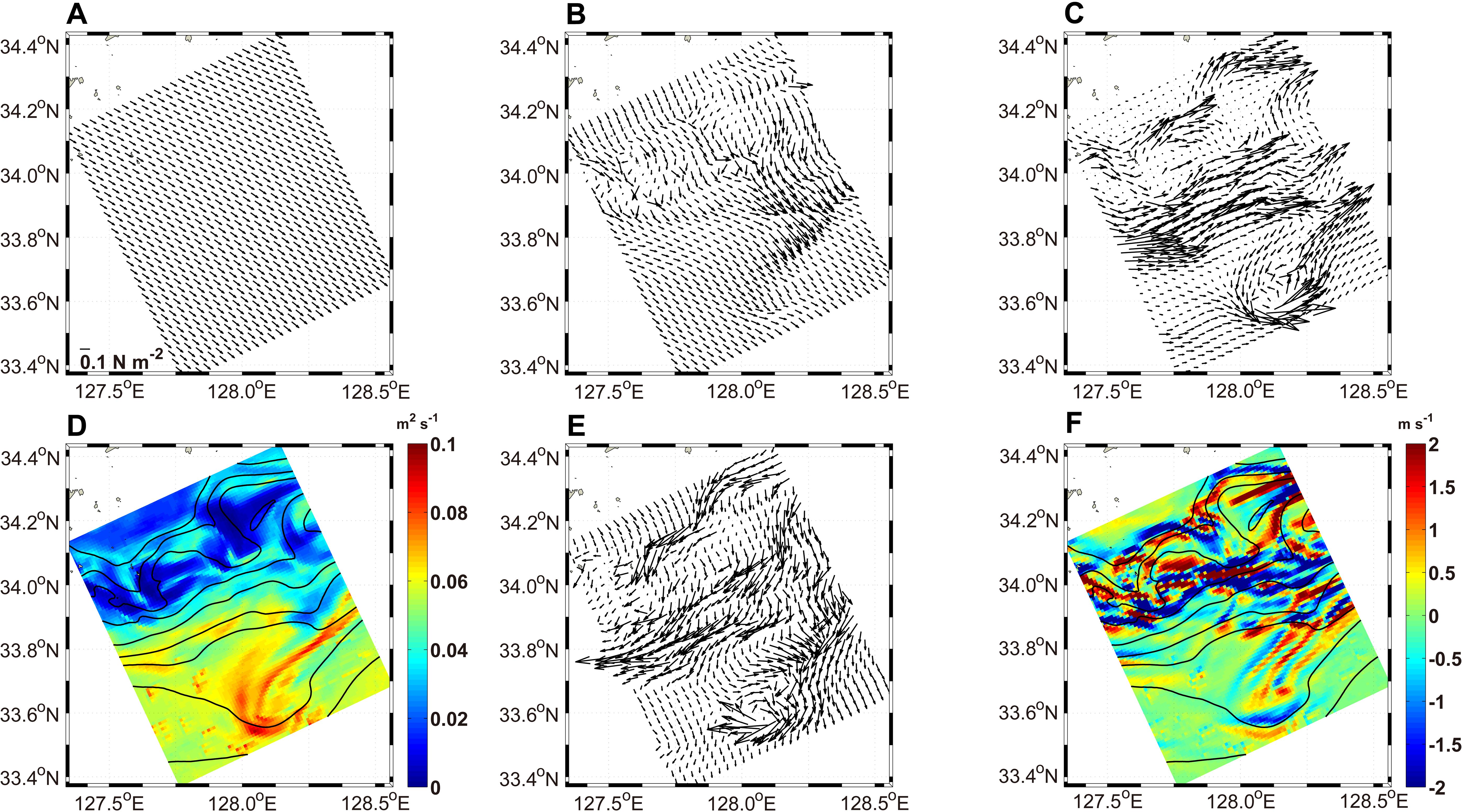
Figure 13. Horizontal distribution of the (A) surface wind stress $\overrightarrow{{\tau }_w}$, (B) total stress $\overrightarrow{\tau }$, (C) geostrophic stress $\overrightarrow{{\tau }_g}$, (D) vertical eddy viscosity $A_z$, (E) ageostrophic stress $\overrightarrow{{\tau }_a}$, and (F) generalized Ekman pumping velocity $w_p$ at a depth of 10 m on November 14, 2006, in the small black rectangle in (Figure 1B). $w_p$ has been increased by a factor of ${10}^4$.

The Ekman number, $E_k= \sqrt{2 A_z/f } /H$, depends on $A_z$, where $H$ is the characteristic vertical scale of $\overrightarrow{{\tau }_g}$. Geostrophic stress induces ageostrophic stress to counterbalance itself (Xu et al., 2022). This counterbalancing effect becomes more evident with an increase in $E_k$. This dynamic process depends on the vertical structures of the turbulent viscosity and geostrophic flows. Xu et al. (2022) examined the relationship between $\overrightarrow{{\tau }_a}$ and $\overrightarrow{{\tau }_g}$ at a front center in an idealized study. According to their results, as the Ekman number increased in both the vertically uniform $A_z$ and varying $A_z$ experiments, $\overrightarrow{{\tau }_a}$ increased and the influence of $\overrightarrow{{\tau }_g}$ on $\overrightarrow{\tau }$ decreased. The effect of $\overrightarrow{{\tau }_g}$ (representing the lateral buoyancy effect) on the horizontal distribution of $\overrightarrow{\tau }$ was significantly weak because the strong westward $\overrightarrow{{\tau }_a}$ offset the strong eastward $\overrightarrow{{\tau }_g}$ along the front (Figures 13B, C, E). $\overrightarrow{{\tau }_g}$ is balanced by $\overrightarrow{{\tau }_a}$ (representing the vertical turbulent mixing effect) along the strong frontal zone (Gula et al., 2014). The distribution of $\overrightarrow{\tau }$ was similar to those of both $\overrightarrow{{\tau }_a}$ and $\overrightarrow{{\tau }_w}$ in the regions outside of the frontal regions because the influence of $\overrightarrow{{\tau }_g}$ was significantly weak (Figure 13E). This spatial distribution of $\overrightarrow{{\tau }_a}$ was affected by that of $\overrightarrow{{\tau }_g}$ because a nearly spatially uniform $\overrightarrow{{\tau }_w}$ is weaker than a spatially varying $\overrightarrow{{\tau }_g}$. The spatial variation of $A_z$ also contributed to the spatial distribution and magnitude of $\overrightarrow{{\tau }_a}$; however, its influence was significantly weaker than that of $\overrightarrow{{\tau }_g}$.

In general, positive and negative curls of stress lead to the convergence and divergence of currents in the surface mixed layer, respectively, in the Northern Hemisphere (Cronin and Tozuka, 2016; Wenegrat and McPhaden, 2016; Yang et al., 2021a; Xu et al., 2022). The generalized Ekman pumping velocity $w_p$ induced by the turbulent thermal balance is given by Equation 12:

$\begin{array}{ll}{w}_p(x,y,z)=-\frac{1}{f {\rho }_0 } \widehat{\mathit{k}} ·(\nabla \times \overrightarrow{{\tau }_w}-\nabla \times \overrightarrow{\tau } )& (12)\end{array}$

The $w_p$ at a depth of 10 m was strong north of 33.9°N where the vertical velocity w was also strong (Figures 11E, 13F). The distribution of vertical velocity $w_p$ had striped and speckled submesoscale patterns consisting of positive and negative values (Figure 13F). Although the $w_p$ at a depth of 10 m was stronger than vertical velocity w, the upwelling and downwelling distribution of $w_p$ was similar to that of w (Figures 11E, 13F).

On November 23, the southwestward $\overrightarrow{{\tau }_w}$ was relatively strong over the study area, with the magnitude of the wind stress 3.3 times larger than that on November 14 (Figures 13A, 14A). $\overrightarrow{{\tau }_a}$ was dominated by $\overrightarrow{{\tau }_w}$ (Figure 14E). $\overrightarrow{{\tau }_g}$ was significantly weaker than that on November 14 (Figure 14C) because the water column was vertically stabilized due to the northward advection of the low-density TWCW. This also significantly weakened ${\nabla }_{h}b$ in Equation 10 at a depth of 10 m. During this period, $\overrightarrow{\tau }$ was nearly equivalent to $\overrightarrow{{\tau }_a}$ in Equation 12 (Figures 14B, E). The horizontal gradient of $A_z$ between onshore and offshore across the thermohaline front became smaller than that during the up-front wind event (Figure 14D). The Ekman spiral in currents within the Ekman layer fully develops within 11–13 h in the KS (Yoshikawa et al., 2007). Due to the strong northeasterly winds from November 22 to 23 (Figure 10A), the surface Ekman depth increased. The duration of the up-front wind was sufficient for the Ekman layer to develop in the study area. The $w_p$ at a depth of 10 m was significantly weaker than that during the down-front wind event (Figure 14F). The relatively weak vertical velocity (w) during the up-front wind event was insufficient to induce strong vertical motion and submesoscale features (Figures 11H, 14F).

Figure 14

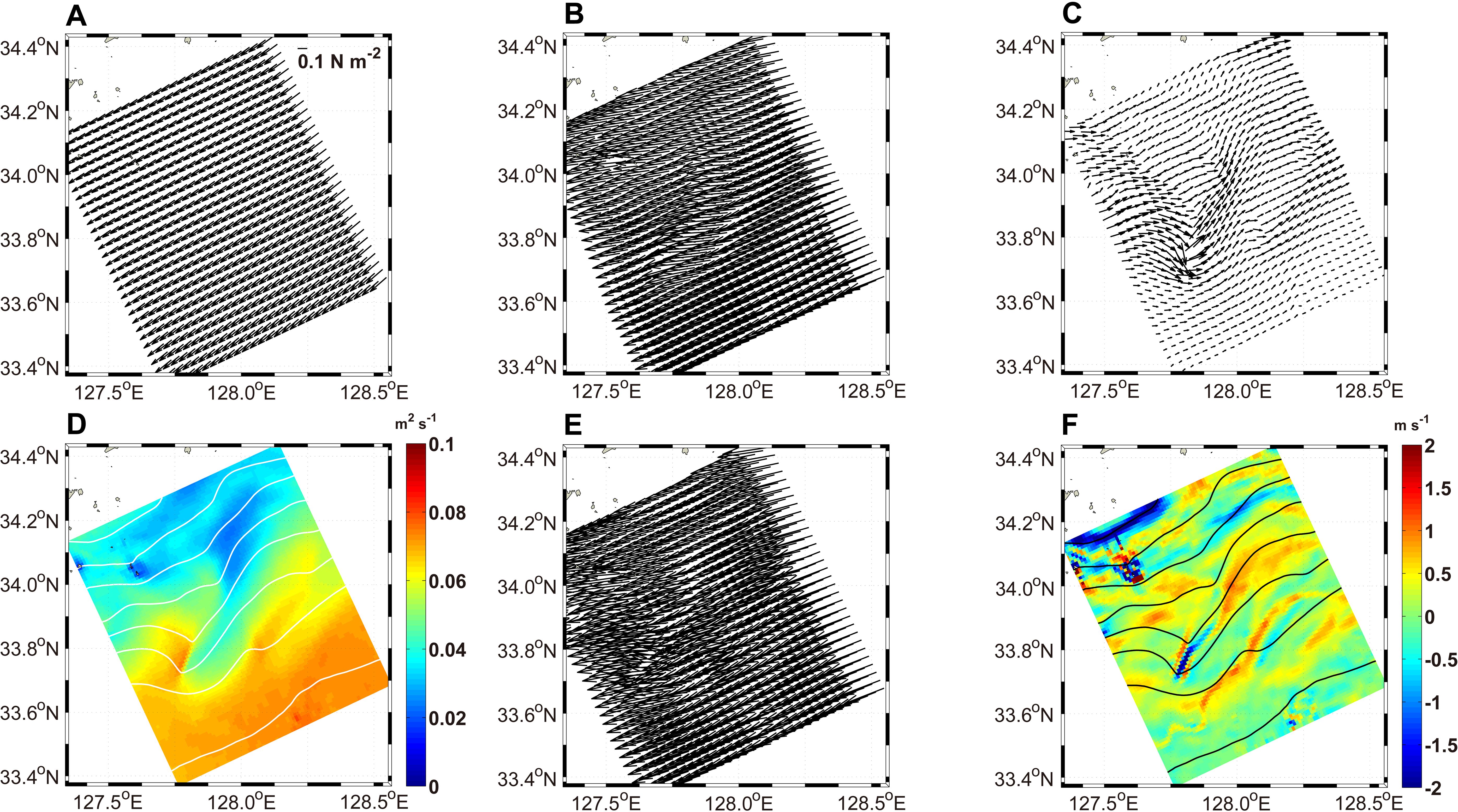
Figure 14. Horizontal distribution of the (A) surface wind stress $\overrightarrow{{\tau }_w}$, (B) total stress $\overrightarrow{\tau }$, (C) geostrophic stress $\overrightarrow{{\tau }_g}$, (D) vertical eddy viscosity $A_z$, (E) ageostrophic stress $\overrightarrow{{\tau }_a}$, and (F) generalized Ekman pumping velocity $w_p$ at a depth of 10 m on November 23, 2006, in the small black rectangle in (Figure 1B). $w_p$ has been increased by a factor of ${10}^4$.

4 Discussion

4.1 Ageostrophic vertical motion and nutrient supply

Frictional processes in the surface boundary layer strongly contribute to the generation of ageostrophic secondary circulation and associated vertical tracer transport (Gula et al., 2014; Wenegrat and McPhaden, 2016; Yang et al., 2021a). Vertical velocity is induced even under a uniform or zero wind field due to the horizontal variability of surface geostrophic currents, surface geostrophic vorticity, and turbulent viscosity (Stern, 1965; Thomas and Rhines, 2002; Mahadevan and Tandon, 2006; Zhang et al., 2019; Yang et al., 2021b; Xu et al., 2022). This ageostrophic secondary circulation is known to supply nutrients to the euphotic layer (Thomas et al., 2008; Levy et al., 2001; Oguz et al., 2015).

Previous studies have reported that the upward velocity in submesoscale processes can exceed 9 $.3\times {10}^{-4}$ m s^-1 (80 m d^-1) in unstable baroclinic jets. Levy et al. (2001) compared the evolution of phytoplankton production and subduction at different horizontal scales using large-scale (i.e., a horizontal grid spacing of 10 km), mesoscale (a horizontal spacing of 6 km), and submesoscale (a horizontal spacing of 2 km) models. Their experiment results suggested that nitrates in the aphotic layer were supplied to the euphotic layer through baroclinic instability. Furthermore, nitrate was more actively supplied to the euphotic layer in the submesoscale model experiment than in the mesoscale model experiment. In the present study, the maximum upward vertical velocity at a depth of 10 m was $6.3\times {10}^{-4}$ m s^-1 ($\sim$54 m d^-1), which was lower than the upward vertical velocity reported by previous studies ($\sim 100$ m d^-1; Levy et al., 2001; Thomas et al., 2008; Oguz et al., 2015). However, the upward vertical velocity maximum at depths from 20 m to 40 m exceeded $10.0\times {10}^{-4}$ m s^-1; in particular, at a depth of 40 m, it was $11.0\times {10}^{-4}$ m s^-1 (i.e. $\sim$95 m d^-1) at 127.63°E, 34.04°N and at 128.21°E, 33.58°N.

Gula et al. (2014) released neutrally buoyant particles into the area surrounding a cold filament in the Gulf Stream region. These particles were transported from the surface to the bottom of the mixed layer, approximately 100 m deep, and then detrained into the upper thermocline. Approximately 40% of the released particles experienced a vertical mixing event after 30 h. This vertical motion, driven by surface cooling and boundary layer mixing, was particularly noticeable near the filament. In our study area, the strong upward vertical velocity exceeding $10.0\times {10}^{-4}$ m s^-1 could potentially supply nutrients from the ocean interior to the euphotic zone along the filamentary regions.

4.2 Instability and ageostrophic secondary circulation

Son et al. (2010) found that strong vertical shear in the mean flow within the pycnocline induced baroclinic instability in the KS. The mean flow they referred to may primarily be geostrophic flow. Their findings revealed that intrusions of water masses between the KCW and TWCW occur along isopycnal surfaces within the pycnocline, leading to vertical inversions in the temperature and salinity profiles. Vertical shear of geostrophic stress can generate ageostrophic secondary circulation without the influence of wind stress forcing (Wenegrat and McPhaden, 2016; Xu et al., 2022). Although Son et al. (2010) did not directly measure vertical velocity or discuss ageostrophic secondary circulation, they suggested that vertical velocity induced by vertical shear in the mean flow could trigger baroclinic instability. This vertical velocity might be associated with ageostrophic secondary circulation induced by geostrophic stress. As a result, it is possible that cross-frontal mixing between the KCW and TWCW within the pycnocline, as observed by Son et al. (2010), is generated by ageostrophic secondary circulation induced by geostrophic shear stress.

5 Conclusion

The development and dissipation of frontal instability and submesoscale features along a surface thermal front in the KS in November 2006 were observed based on SST gradient patterns in satellite data. During the evolution period of the instability along the surface thermal front, down-front winds over the KS enhanced the horizontal thermal gradient and intensified the vertical geostrophic stress along the front. Wind stress affected both the horizontal and vertical circulations. The combined effects of wind and geostrophic vertical stresses induced the divergence of the ageostrophic current. During this down-front wind event, strong submesoscale instability developed because vertical velocities were enhanced by the divergence and convergence of ageostrophic currents. These vertical velocities increased the EAPE along the filamentary region. This suggests that the buoyancy flux plays an active role in the filamentary region, intensifying the development of filaments, submesoscale features, and the meandering of the thermohaline front. The primary results of this study indicate that the stress induced by the frictional response within the ocean boundary layer was as important as surface wind stress. Stress sources within the ocean interior associated with viscosity generated ageostrophic currents and their divergence led to vertical motion in the autumn KS region. This resulted in numerous submesoscale features at the surface of the KS during autumn. When the wind direction shifted up-front over the KS, the surface thermal front weakened. The wind stress was dominant over vertical geostrophic stress over the KS, leading to the weaker divergence of the ageostrophic current and reduced vertical velocity. The advection of the TWCW toward the shore due to Ekman transport stabilized the water column, causing the thermohaline front to flatten and the submesoscale features to decay.

This study mainly focused on comparing dynamic processes in the development and decay of submesoscale features during down-front and up-front wind periods. However, it did not examine in detail the growth and decay of energy that sustains submesoscale features along the thermohaline front. During down-front wind periods, the EAPE increased, likely due to conversion from the mean kinetic energy and the APE. This energy conversion process has been explored in many previous studies (Ivchenko et al., 1997; Marchesiello et al., 2003; Durski and Allen, 2005; Halo et al., 2014; Kang and Curchitser, 2015). Future research that includes an analysis of energy conversion would enhance the understanding of the dynamic relationship between baroclinic instability and the development of submesoscale features, as well as their sequential evolution and decay in the thermohaline frontal region of the KS.

Data availability statement

The raw data supporting the conclusions of this article will be made available by the authors, without undue reservation.

Author contributions

JK: Formal Analysis, Investigation, Visualization, Writing – original draft, Writing – review & editing. BC: Conceptualization, Formal Analysis, Funding acquisition, Investigation, Methodology, Writing – original draft, Writing – review & editing. SL: Conceptualization, Investigation, Methodology, Writing – review & editing. YS: Conceptualization, Investigation, Methodology, Writing – review & editing.

Funding

The author(s) declare that financial support was received for the research and/or publication of this article. This research was supported by the Korea Institute of Marine Science & Technology Promotion (KIMST) funded by the Ministry of Oceans and Fisheries (RS-2022-KS221544) and the Basic Science Research Program through the National Research Foundation of Korea (NRF), the Ministry of Education (2020R1A2C1014678).

Conflict of interest

Author YS was employed by the company Geosystem Research Corporation.

The remaining authors declare that the research was conducted in the absence of any commercial or financial relationships that could be constructed as a potential conflict of interest.

Generative AI statement

The author(s) declare that no Generative AI was used in the creation of this manuscript.

Publisher’s note

All claims expressed in this article are solely those of the authors and do not necessarily represent those of their affiliated organizations, or those of the publisher, the editors and the reviewers. Any product that may be evaluated in this article, or claim that may be made by its manufacturer, is not guaranteed or endorsed by the publisher.

References

Cronin M., Tozuka T. (2016). Steady state ocean response to wind forcing in extratropical frontal regions. Sci. Rep. 6, 28842. doi: 10.1038/srep28842

PubMed Abstract | Crossref Full Text | Google Scholar

Della Penna A., Gaube P. (2019). Overview of (sub)mesoscale ocean dynamics for the NAAMES field program. Front. Mar. Sci. 6. doi: 10.3389/fmars.2019.00384

Crossref Full Text | Google Scholar

Donlon C. J., Martin M., Stark J. D., Roberts-Jones J., Fiedler E., Wimmer W. (2012). The operational sea surface temperature and sea ice analysis (OSTIA). Remote Sens. Environ. 116, 140–158. doi: 10.1016/j.rse.2010.10.017

Crossref Full Text | Google Scholar

Durski S. M., Allen J. S. (2005). Finite-amplitude evolution of instabilities associated with the coastal upwelling front. J. Phys. Oceanogr. 35, 1606. doi: 10.1175/JPO2762.1

Crossref Full Text | Google Scholar

Fairall C. W., Bradley E. F., Rogers D. P., Edson J. B., Young G. S. (1996). Bulk parameterization of air-sea fluxes for Tropical Ocean-Global Atmosphere Coupled-Ocean Atmosphere Response Experiment. J. Geophys. Res. 101, 3747–3764. doi: 10.1029/95JC03205

Crossref Full Text | Google Scholar

Gill A. E. (1982). Atmosphere-ocean dynamics. San Diego, California, USA: Academic Press.

Google Scholar

Gong Y. (1971). A study on the South Korean coastal front (in Korean with English abstract). J. Korean Soc Oceanol. 1, 25–36.

Google Scholar

Gula J., Molemaker M. J., McWilliams J. C. (2014). Submesoscale cold filaments in the Gulf Stream. J. Phys. Oceanogr. 44, 2617–2643. doi: 10.1175/JPO-D-14-0029.1

Crossref Full Text | Google Scholar

Haidvogel D. B., Arango H. G., Hedstrom K., Beckmann A., Malanotte-Rizzoli P., Shchepetkin A. F. (2000). Model evaluation experiments in the North Atlantic Basin: Simulations in nonlinear terrain-following coordinates. Dyn. Atmos. Oceans 32, 239–281. doi: 10.1016/S0377-0265(00)00049-X

Crossref Full Text | Google Scholar

Halo I., Penven P., Backeberg B., Ansorge I., Shillington F., Roman R. (2014). Mesoscale eddy variability in the southern extension of the East Madagascar Current: Seasonal cycle, energy conversion terms, and eddy mean properties. J. Geophys. Res. Oceans 119, 7324–7356. doi: 10.1002/2014JC009820

Crossref Full Text | Google Scholar

Huh O. K. (1982). Satellite observations and annual cycle of surface circulation in the Yellow Sea, East China Sea and Korea Strait. Mer. 20, 210–222.

Google Scholar

Ikeda M. (1985). Wind effect on a front over the continental shelf slope. J. Geophys. Res. 90, 9108–9118. doi: 10.1029/JC090iC05p09108

Crossref Full Text | Google Scholar

Ivchenko V. O., Treguier A. M., Best S. E. (1997). A kinetic energy budget and internal instabilities in the fine resolution Antarctic model. J. Phys. Oceanogr. 27, 5–22. doi: 10.1175/1520-0485(1997)027<0005:AKEBAI>2.0.CO;2

Crossref Full Text | Google Scholar

Jhun J. G., Lee E. J. (2004). A new East Asian winter monsoon index and associated characteristics of the winter monsoon. J. Climate 17, 711–726. doi: 10.1175/1520-0442(2004)017<0711:ANEAWM>2.0.CO;2

Crossref Full Text | Google Scholar

Johannessen J. A., Kudryavtsev V., Akimov D., Eldevik T., Winther N., Chapron B. (2005). On radar imaging of current features: 2. Mesoscale eddy and current front detection. J. Geophys. Res. Ocean 110, C07017. doi: 10.1029/2004JC002802

Crossref Full Text | Google Scholar

Kang D., Curchitser E. N. (2015). Energetics of Eddy-Mean flow interactions in the Gulf Stream Region. J. Phys. Oceanogr. 45, 1103–1120. doi: 10.1175/JPO-D-14-0200.1

Crossref Full Text | Google Scholar

Kim Y. S. (1996). Estimate of heat flux in the East China Sea (in Korean with English abstract). J. Korean Fish. Soc 29, 84–91.

Google Scholar

Large W. G., Pond S. (1981). Open ocean momentum flux measurements in moderate to strong wind. J. Phys. Oceanogr. 11, 324–336. doi: 10.1175/1520-0485(1981)011<0324:OOMFMI>2.0.CO;2

Crossref Full Text | Google Scholar

Lee S. H., Choi B. J. (2015). Vertical structure and variation of currents observed in autumn in the Korea Strait. Ocean Sci. J. 50, 163–182. doi: 10.1007/s12601-015-0013-5

Crossref Full Text | Google Scholar

Lee J. C., Na J. Y., Chang S. D. (1984). Thermohaline structure of the shelf front in the Korea Strait in early winter. J. Oceanogr. Soc Korea 19, 56–67.

Google Scholar

Levy M., Klein P., Treguier A.-M. (2001). Impact of sub-mesoscale physics on production and subduction of phytoplankton in an oligotrophic regime. J. Mar. Res. 59, 535–565. doi: 10.1357/002224001762842181

Crossref Full Text | Google Scholar

Levy M., Klein P., Treguier A.-M., Iovino D., Madec G., Masson S., et al. (2010). Modifications of gyre circulation by sub-mesoscale physics. Ocean Model. 34, 1–15. doi: 10.1016/j.ocemod.2010.04.001

Crossref Full Text | Google Scholar

Mahadevan A. (2006). Modeling vertical motion at ocean fronts: Are nonhydrostatic effects relevant at submesoscales? Ocean Model. 14, 222–240. doi: 10.1016/j.ocemod.2006.05.005

Crossref Full Text | Google Scholar

Mahadevan A., Archer D. (2000). Modeling the impact of fronts and mesoscale circulation on the nutrient supply and biogeochemistry of the upper ocean. J. Geophys. Res. Ocean 105, 1209–1225. doi: 10.1029/1999JC900216

Crossref Full Text | Google Scholar

Mahadevan A., Tandon A. (2006). An analysis of mechanisms for submesoscale vertical motion at ocean fronts. Ocean Model. 14, 241–256. doi: 10.1016/j.ocemod.2006.05.006

Crossref Full Text | Google Scholar

Marchesiello P., McWilliams J. C., Shchepetkin A. (2003). Equilibrium structure and dynamics of the California Current System. J. Phys. Oceanogr. 33, 753–783. doi: 10.1175/1520-0485(2003)33<753:ESADOT>2.0.CO;2

Crossref Full Text | Google Scholar

Matsumoto K., Takanezasa T., Ooe M. (2000). Ocean tide models developed by assimilating TOPEX/POSEIDON altimeter data into hydrodynamical model: a global model and a regional model around Japan. J. Oceanogr. 56, 567–581. doi: 10.1023/A:1011157212596

Crossref Full Text | Google Scholar

McWilliams J. C. (2017). Submesoscale surface fronts and filaments: secondary circulation, buoyancy flux, and frontogenesis. J. Fluid Mech. 823, 391–432. doi: 10.1017/jfm.2017.294

Crossref Full Text | Google Scholar

Mellor G. L., Yamada T. (1982). Development of a turbulence closure model for geophysical fluid problems. Rev. Geophys. Space Phys. 20, 851–875. doi: 10.1029/RG020i004p00851

Crossref Full Text | Google Scholar

Na J. Y., Han S. K., Cho K. D. (1990). A study on sea water and ocean current in the sea adjacent to Korea peninsula-expansion of coastal waters and its effect on temperature variations in the South Sea of Korea (in Korean with English abstract). Bull. Korean Fish. Soc 23, 267–279.

Google Scholar

O’ Sullivan D., Dunkerton T. J. (1995). Generation of inertia-gravity waves in a simulated life cycle of baroclinic instability. J. Atoms. Sci. 52, 3695–3716. doi: 10.1175/1520-0469(1995)052<3695:GOIWIA>2.0.CO;2

Crossref Full Text | Google Scholar

Oguz T., Macias D., Tinore J. (2015). Ageostrophic frontal processes controlling phytoplankton production in the Catalano Balearic Sea (Western Mediterranean). PloS One 10, e0129045. doi: 10.1371/journal.pone.0129045

PubMed Abstract | Crossref Full Text | Google Scholar

Park K. A., Park J. E., Choi B. J., Lee S. H., Lee E. I., Byun D. S., et al. (2014) An analysis of oceanic current maps of the Yellow Sea and the East China Sea in secondary school science textbooks (in Korean with English abstract). J. Korean Earth Sci. Soc 35, 439–466. doi: 10.5467/JKESS.2014.35.6.439

Crossref Full Text | Google Scholar

Pond S., Pickard G. L. (1983). Introductory dynamical oceanography. Oxford: Pergamon Press.

Google Scholar

Rosso I., Hogg A. M. C., Strutton P. G., Kiss A. E., Matear R., Klocker A., et al. (2014). Vertical transport in the ocean due to sub-mesoscale structures: Impacts in the Kerguelen region. Ocean Model. 80, 10–23. doi: 10.1016/j.ocemod.2014.05.001

Crossref Full Text | Google Scholar

Ruiz S., Claret M., Pascual A., Olita A., Troupin C., Capet A., et al. (2019). Effects of oceanic mesoscale and submesoscale frontal processes on the vertical transport of phytoplankton. J. Geophys. Res. Ocean 124, 5999–6014. doi: 10.1029/2019JC015034

Crossref Full Text | Google Scholar

Seo S. N. (2008). Digital 30sec gridded bathymetric data of korea marginal seas-korBathy30s (in korean with english abstract). J. Korean Soc Coast Ocean Eng. 20, 110–120.

Google Scholar

Seo G. H., Cho Y. K., Choi B. J. (2014). Variations of heat transport in the northwestern Pacific marginal seas inferred from high-resolution reanalysis. Prog. Oceanogr. 121, 98–108. doi: 10.1016/j.pocean.2013.10.005

Crossref Full Text | Google Scholar

Shchepetkin A. F., McWilliams J. C. (2005). The Regional Oceanic Modeling System (ROMS): A split-explicit, free-surface, topography-following-coordinate oceanic model. Ocean Model. 9, 347–404. doi: 10.1016/j.ocemod.2004.08.002

Crossref Full Text | Google Scholar

Son Y. T. (2008). A study on frontal variation and characteristics in the South Sea of Korea in cooling period. Ph.D. thesis (Gunsan: Kunsan National University).

Google Scholar

Son Y. T., Lee S. H., Choi B. J., Lee J. C. (2010). Frontal structure and thermohaline intrusions in the South Sea of Korea from observed data and a relocation method. J. Geophys. Res. 115, C02011. doi: 10.1029/2009JC005266

Crossref Full Text | Google Scholar

Stern M. (1965). Interaction of a uniform wind stress with a geostrophic vortex. Deep Sea Res. Oceanogr. Abstr. 12, 355–367. doi: 10.1016/0011-7471(65)90007-0

Crossref Full Text | Google Scholar

Thomas L. N., Lee C. M. (2005). Intensification of ocean fronts by down-front winds. J. Phys. Oceanogr. 35, 1086–1102. doi: 10.1175/JPO2737.1

Crossref Full Text | Google Scholar

Thomas L. N., Rhines P. B. (2002). Nonlinear stratified spin up. J. Fluid Mech. 473211–244. doi: 10.1017/S0022112002002367

Crossref Full Text | Google Scholar

Thomas L. N., Tandon A., Mahadevan A. (2008)Submesoscale processes and dynamics in Ocean modeling in an eddying regime, volume 177 of geophysical monograph series. Eds. Hecht M., Hasumi H. (Hoboken NJ: Wiley)17–38. doi: 10.1029/177GM04

Crossref Full Text | Google Scholar

Trenberth K. E., Large W. G., Olson J. G. (1990). The mean annual cycle in global ocean wind stress. J. Phys. Oceanogr. 20, 1742–1760. doi: 10.1175/1520-0485(1990)020<1742:TMACIG>2.0.CO;2

Crossref Full Text | Google Scholar

Wenegrat J. O., McPhaden M. J. (2016). Wind, waves, and fronts: frictional effects in a generalized Ekman model. J. Phys. Oceanogr. 46, 371–394. doi: 10.1175/JPO-D-15-0162.1

Crossref Full Text | Google Scholar

Xu F., Jing Z., Yang P., Zhou S. (2022). Vertical motions driven by geostrophic stress in surface boundary layer under a finite Ekman number regime. J. Phys. Oceanogr. 52, 3033–3047. doi: 10.1175/JPO-D-21-0263.1

Crossref Full Text | Google Scholar

Yang P., Jing Z., Sun B., Wu L., Qiu B., Chang P., et al. (2021b). On the upper-ocean vertical eddy heat transport in the Kuroshio extension. Part II: Effects of air-sea interactions. J. Phys. Oceanogr. 51, 3297–3312. doi: 10.1175/JPO-D-20-0068.s1

Crossref Full Text | Google Scholar

Yang P., Jing Z., Sun B., Wu L., Qiu B., Chang P., et al. (2021a). On the upper-ocean vertical eddy heat transport in the Kuroshio Extension. Part I: Variability and dynamics. J. Phys. Oceanogr. 51, 229–246. doi: 10.1175/JPO-D-20-0068.1

Crossref Full Text | Google Scholar

Yoshikawa Y., Matsuno T., MArubayashi K., Fukudome K. (2007). A surface velocity spiral observed with ADCP and HF radar in the Tsushima Strait. J. Geophys. Res. 112, C06022. doi: 10.1029/2006JC003625

Crossref Full Text | Google Scholar

Zhang X., Dai H., Zhao J., Yin H. (2019). Generation mechanism of an observed submesoscale eddy in the chukchi Sea. Deep Sea Res. Part I: Oceanographic Res. Papers 148, 80–87. doi: 10.1016/j.dsr.2019.04.015

Crossref Full Text | Google Scholar