Vector tracking loop of shipborne satellite navigation receiver based on Kalman filter-divided difference filter for anti-interference enhancement

Due to the complex and ever-changing maritime environment, ships heavily rely on stable and reliable navigation systems during their voyages to ensure safe and efficient navigation. However, during maritime navigation, satellite navigation signals are often subject to interference and obstruction, leading to degraded positioning accuracy or untrustworthy navigation data. To address the pressing need for high-precision and reliable navigation in maritime applications, this paper proposes a bidirectional smoothing filter vector tracking loop (VTL) structure based on a combination of Kalman filter (KF) and a Divided Difference filter (DDF). This approach enhances the responsiveness of the Kalman filter under high-noise conditions, and significantly improves the accuracy and robustness of the navigation system through bidirectional collaborative filtering. In practical shipborne navigation experiments, the proposed method was compared with the traditional Scalar Tracking Loops (STL), traditional VTL, and KF-based VTL approaches. The results demonstrate that the proposed method offers significant improvements in horizontal positioning and velocity accuracy. Compared with the KF-based VTL method, the proposed approach achieved an 83.20% enhancement in the positioning accuracy and a 60.00% improvement in the horizontal velocity accuracy.

1 Introduction

Navigation safety has always been the paramount concern for mariners. Given the complex and unpredictable nature of the maritime environment, factors such as weather, tides, ocean currents, and other uncertainties pose significant challenges to safe navigation. As a result, ships heavily depend on stable and reliable navigation systems during their voyages. Advanced navigation technology not only delivers accurate positioning, heading, and speed information but also assists vessels in avoiding potential hazards and enhancing navigation efficiency. Moreover, the integration and intelligent evolution of modern navigation systems enable ships to maintain safe passage even in adverse weather conditions, low visibility, or intricate waterways. These advanced systems provide crucial support for maritime safety. As a result, they help protect the crew, secure the cargo, and ensure the stability of shipping operations.

According to the performance standards for shipborne radio navigation receivers set out in the IMO’s MSC.401(95) resolution, the specifications outline the requirements for navigation performance and reliability of shipborne satellite radio navigation systems (Lacarra et al., 2019). The standards specify that shipborne radio navigation systems must remain stable even when exposed to electromagnetic interference occurring either inside or outside the vessel. In addition, they should be able to continuously and reliably deliver accurate navigation data.

With the rapid development of global shipping, the accuracy and reliability of ship navigation systems have become increasingly important. Traditional navigation systems face numerous challenges in complex and variable environments. These difficulties arise from the influence of maritime conditions and obstacles such as bridges, which can disrupt signal reception and reduce positioning accuracy (Niu et al., 2024). As the core technology for modern ship navigation, satellite navigation systems directly affect navigation safety and efficiency. However, issues such as signal interference, obstructions, and multipath effects in complex environments often lead to unstable navigation signals and decline in system accuracy, thereby affecting the normal operation of ships (Reda et al., 2024). Therefore, future development of maritime navigation technology should focus on achieving higher precision and reliability. This is not only an essential requirement for improving navigation safety and efficiency. It also serves as a critical safeguard against the challenges posed by complex marine environments and extreme weather conditions (Zhang et al., 2021). Chen et al. proposed a path planning method based on Parallel Dense neural Network (PDNet) to meet the complex path data collection requirements of Autonomous Underwater Vehicle (AUV). Additionally, they constructed a three-dimensional marine environment model using real marine current data, which can fulfill the diverse mission planning and data collection needs of AUVs (Chen et al., 2024c). High-precision navigation technology can provide ships with more accurate positioning and route planning, whereas highly reliable systems ensure that navigation equipment remains stable even in the presence of signal interference or harsh environments (Perera and Guedes Soares, 2015). Therefore, research on high-precision and highly reliable shipborne navigation technology tailored to complex environments with signal interference is of utmost significance.

Satellite navigation receivers achieve a stable navigation output by continuously tracking radio frequency signals from navigation satellites. Based on the independence of signals within the tracking channels, signal-tracking loop methods can be categorized into scalar tracking loops (STL) and vector tracking loops (VTL). Scalar tracking is currently the most commonly used signal-tracking method for navigation receivers. The key feature is that the signal channels for each satellite operate independently without mutual interference. In environments with good signal quality and minimal interference, scalar tracking delivers an excellent signal-tracking performance. Additionally, owing to its low computational complexity and simple structure, scalar tracking is widely adopted in various types of navigation receivers (Gao et al., 2024). By contrast, the vector tracking method processes all satellite signals in a single integrative filter, thereby establishing interconnections among the satellite signals. It leverages the relationship between the satellite signal channels to estimate the navigation state. This estimated information can be used to predict the motion characteristics of the receiver. It can also be fed back into each signal-tracking channel to assist in the stable tracking of the signal loop (Sun et al., 2017). This approach enhances the stability and robustness of the vector tracking signal loop, enabling reliable signal channel tracking even in complex interference environments, thereby ensuring navigation accuracy (Zhao et al., 2011). Therefore, the vector tracking method has attracted widespread attention in the academic community. This is due to its excellent anti-interference capability and outstanding tracking performance under weak signal conditions.

As the demand for high reliability and system stability in navigation systems continues to grow, the focus of navigation technology research has evolved accordingly. Over the past decade, the vector tracking loop for satellite navigation signals has gradually become a hot topic in academia owing to its superior anti-interference capabilities and robust performance in weak-signal environments. Researchers have been improving vector tracking methods, continually exploring their potential applications in complex environments to meet the higher requirements of modern navigation systems in terms of accuracy, reliability and stability. Xu et al. proposed a method for detecting and correcting non-line-of-sight (NLOS) errors in satellite signals based on vector tracking. This approach detects NLOS errors within the loop and corrects them before the navigation estimator, thereby effectively improving the positioning accuracy of the navigation system (Xu et al., 2020). Jia et al. analyzed four potential error sources in vector tracking loops and proposed a robust signal vector tracking loop structure based on these findings (Jia et al., 2024). To address the issue of potential spoofing attacks in GNSS navigation systems, Zhou et al. proposed a detection-estimation-correction loop structure based on vector tracking (Zhou et al., 2023). To verify task planning in complex scenarios and the reliability of the system in complex environments, Chen et al. thoroughly studied the dynamic real-time technology of unmanned systems and proposed the robust VD-DDQN algorithm (Chen et al., 2024b). By leveraging the Virtual Autocorrelation Function (VACF) method, they successfully restored accurate navigation and positioning results, ensuring system integrity and reliability (Zhou et al., 2023). Abedi et al. introduced technical improvements to the computational process of vector tracking to address the challenge of the high computational complexity of vector tracking. Their approach significantly reduced the computational load while maintaining nearly the same level of accuracy, thereby enhancing the real-time performance of the method (Abedi and Mosavi, 2022). To enhance the security of maritime communication and the reliability of data transmission, Chen et al. proposed a joint communication model based on DSF-ISS, effectively improving the security and coverage of maritime network communication (Chen et al., 2024a). In high-dynamic environments, vector tracking methods also demonstrate good performance (Lashley et al., 2009). Building on vector tracking, Tu et al. designed a vector carrier structure for Doppler component calculations, which effectively reduced signal tracking errors under high-dynamic conditions (Tu et al., 2021).

In this study, we build on the excellent performance of the vector tracking method in anti-jamming and weak signal environments. We improve the traditional vector tracking loop structure and propose a new algorithmic framework. This framework is based on a bidirectional smoothing filter that combines the Kalman Filter and the Divided Difference Filter (KF-DDF). The following sections introduce the structure of the proposed algorithm and describe the process of constructing its mathematical model. Finally, they present an analysis of the results obtained from an actual shipborne navigation experiment.

2 Algorithm framework

To enhance the safety of vessels during operation, this paper focuses on reducing the impact of external electromagnetic interference on onboard satellite navigation systems. For this purpose, it proposes a carrier/code loop filter designed specifically for complex electromagnetic environments. The filter combines a forward KF with a backward DDF to improve tracking performance and robustness. This innovative filter design aims to improve the anti-jamming capability and positioning accuracy of shipborne satellite navigation systems under harsh conditions to ensure the safety and reliability of ship navigation.

Based on the proposed KF-DDF carrier/code loop filter, the entire algorithm structure implements the positioning calculation process of the Software-Defined Receiver (SDR). In this process, the software-defined receiver no longer relies on hardware receivers but fully utilizes the flexibility and programmability of the software. By employing efficient algorithms and dynamic filtering strategies, the positioning accuracy and anti-jamming capability were enhanced. Specifically, the KF-DDF carrier/code loop filter, as the core algorithm, combines the advantages of forward Kalman filtering and backward differential filtering, thereby enabling real-time tracking and optimization of the received signals(Q. Zhang et al., 2022). This ensures that the navigation system operates stably in complex electromagnetic environments, thereby improving the robustness of the system. The workflow of the entire algorithm is illustrated in Figure 1 (Hsu et al., 2015; Zhang et al., 2022).

Figure 1

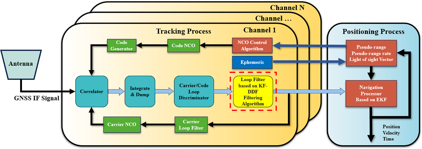
Figure 1. Vector tracking algorithm structure.

Intermediate frequency (IF) signals are first allocated to different vector tracking channels based on the signals received from different satellites (Han et al., 2022). Each tracking channel is responsible for tracking signal from a specific satellite. In each tracking channel, the signal is sent to a correlator for processing. The correlator extracts information such as phase, frequency, and time from the received signal by matching it with a locally generated reference signal (Farhad et al., 2021). The intermediate frequency (IF) signal is then sent to the Integration and Dump (I&D) for integration processing, which eliminates high-frequency noise in the signal and optimizes the signal-to-noise ratio (SNR), thereby enhancing the tracking performance of the signal. Next, the carrier/code discriminator calculates the phase errors of the carrier and pseudo-code, and these errors are used as measurement input parameters for the loop filter. The pseudo-range error and pseudo-range rate error are calculated using the loop filter and used as key measurement parameters for the navigation processor. These are decisive factors affecting the accuracy of the navigation system. Simultaneously, the output of the loop filter serves as the control parameter for the carrier NCO, forming feedback to achieve closed-loop tracking of the signal (Mu and Long, 2021). The navigation filter based on the Extended Kalman filter (EKF) not only computes the current position, velocity, and time information but also estimates the navigation state parameters. By integrating the current satellite ephemeris, it adjusts the control parameters of the pseudo-code NCO, forming a closed-loop control for the pseudo-code signal.

The following sections introduce the basic principles of the proposed method and the design process of its mathematical model.

2.1 KF-DDF GNSS signal-tracking loop

The signal loop filter based on the KF-DDF proposed in this study combines the advantages of both the KF and the DDF. The aim is to improve the accuracy and robustness of the navigation system by leveraging their bidirectional synergy. Specifically, building on forward Kalman filtering, the filter further optimizes the system’s prediction results by applying backward differential filtering to the one-step prediction.

Studies have shown that the Kalman filter can provide an accurate state estimation and demonstrates significant advantages when dealing with linear dynamic models and Gaussian noise systems. In these application scenarios, the Kalman filter continuously optimizes system state estimation through recursive prediction and update steps. Moreover, the Kalman filter operates on the principle of real-time measurement updates and has relatively low computational overhead. These characteristics make it particularly well-suited for systems with high real-time requirements and limited computational resources. Therefore, the Kalman filter is widely applied in fields such as automatic control, navigation, and communication, making it an essential tool for solving complex linear dynamic estimation problems. The loop filter model used in this study generally satisfies the assumptions of the Kalman filter model: the system is linear and the noise follows a Gaussian distribution (Yang et al., 2002).

However, when the system encounters sudden disturbances, the Kalman filter may not respond promptly to changes in the state of the system and adjust the estimates quickly, resulting in a certain degree of latency. This latency arises from the Kalman filter’s reliance on prediction and update mechanisms, which makes it difficult to capture rapid system changes in real-time (Karlgaard and Shen, 2013). When facing sudden disturbances, the filter may require some time to “adapt” to the new system state, leading to temporary degradation in the estimation accuracy. Especially in shipborne satellite navigation systems, when the received electromagnetic signals are interfered with, the state estimation in the signal-tracking loop may deviate significantly from the actual conditions. This deviation not only affects navigation accuracy but also severely weakens the robustness of the system. As a result, the navigation system can become unstable in complex electromagnetic environments or under harsh operating conditions. This instability may ultimately compromise safe and reliable navigation. Therefore, to enhance the anti-jamming capabilities and robustness of the navigation system, it is crucial to propose appropriate optimization strategies to address this latency issue. These strategies should ensure that the system can quickly adjust and restore normal operation when sudden disturbances occur.

To achieve accurate prediction of state variables in the signal loop and reduce the sensitivity of the system state estimation under signal interference, this study implements targeted improvements to the traditional KF system. Specifically, a DDF is introduced to optimize the signal tracking loop, thereby enhancing the system’s performance and stability in complex electromagnetic environments (Karlgaard and Schaub, 2007).

The principle of the DDF is based on predicting the system state by observing the changes between the current measurement and previous measurement (Xia et al., 2022). The core idea of this process is differential processing, which involves modeling changes in the system state rather than relying directly on absolute state values. This method effectively removes noise and random interference, thereby improving the prediction accuracy and system stability. In practical applications, the advantage of the DDF filter lies in its ability to quickly respond to changes in the system state, particularly when faced with sudden disturbances. By using differential processing, the system can effectively suppress the impact of interference on state estimation. In addition, the DDF filter operates recursively during its usage, which makes it particularly suitable for systems that require real-time performance and high accuracy.

The proposed KF-DDF signal-loop filter introduces backward differential filtering after forward filtering. This step further refines the observation vector. Backward differential filtering effectively eliminates or suppresses high-frequency noise. Thus enhances the noise suppression and signal tracking capabilities of the system by analyzing changes in the signal without relying heavily on the system model. Additionally, the filter can capture and correct errors in the system better, significantly improving the accuracy of the prediction results.

2.2 Design of forward KF filter

In the operation of the KF-DDF carrier and pseudo-code joint signal-loop filter, the process starts with forward KF filtering. The design of the mathematical model is as follows. In the designed signal-tracking loop system model, $X_{KF}^i$ represents a four-dimensional observation vector consisting of the pseudo-code phase error $\Delta {\rho }^i$ (rad), carrier phase error $\Delta {\sigma }^i$ (chips), carrier frequency error $\Delta f^i$ (Hz), and carrier frequency rate error $\Delta {\dot{f}}^i$ (Hz/s). $Z_{KF}^i$ represents a two-dimensional measurement vector consisting of the average pseudo-code phase error $\Delta {\overline{\rho }}^i$ and average carrier phase error $\Delta {\overline{\sigma }}^i$. The system model in the discrete state can be simplified as follows (Sun et al., 2014; Yang et al., 2021) (Equations 1–4).

$\begin{array}{ll}{X}_{KF,k}^i={\Phi }_{KF,k/k-1}{X}_{KF,k-1}^i+W_{KF,k}^i& (1)\end{array}$

$\begin{array}{ll}{Z}_{KF,k}^i=H_{KF,k}{X}_{KF,k}^i+V_{KF,k}^i& (2)\end{array}$

$\begin{array}{ll}{X}_{KF}^i=[\Delta {\rho }^i,\Delta {\sigma }^i,\Delta f^i,\Delta {\dot{f}}^i]& (3)\end{array}$

$\begin{array}{ll}{Z}_{KF}^i={[\begin{array}{cc}\Delta {\overline{\rho }}^i& \Delta {\overline{\sigma }}^i\end{array}]}^T& (4)\end{array}$

In the mathematical model of the system (Equation 1), ${\Phi }_{KF}$ represents the system’s state transition matrix for one step, $W_{KF}$ is the system’s noise vector, $H_{KF}$ is the system’s measurement matrix, and $V_{KF}$ is the measurement noise vector (Equation 2). Typically, both the system noise $W_{KF}$ and measurement noise $V_{KF}$ are zero-mean Gaussian white noise, following a normal distribution. In addition, the notation $i$ in the formula represents the current number of satellite tracking channels being processed. These physical quantities can be abstractly described as follows (Heyne, 2007; Tripathy et al., 2010) (Equations 5–8):

$\begin{array}{ll}{\Phi }_{KF}=\left[\begin{array}{cccc}1& 0& \beta T& \frac{1}{2}\beta T^2\\ 0& 1& 2\pi T& \pi T^2\\ 0& 0& 1& T\\ 0& 0& 0& 1\end{array}\right]& (5)\end{array}$

$\begin{array}{ll}{H}_{KF}=\left[\begin{array}{cccc}1& 0& -\frac{1}{2}\beta T& \frac{1}{6}\beta T^2\\ 0& 1& -\pi T& \frac{1}{3}\pi T^2\end{array}\right]& (6)\end{array}$

$\begin{array}{ll}\begin{array}{ll}E[W_{KF,k}]\mathrm{=0}\hfill & E[W_{KF,k}{(W_{KF,k})}^T]=Q_{KF,k}\hfill \end{array}& (7)\end{array}$

$\begin{array}{ll}\begin{array}{ll}E[V_{KF,k}]=0\hfill & E[V_{KF,k}{(V_{KF,k})}^T]=R_{KF,k}\hfill \end{array}& (8)\end{array}$

where (Equations 5, 6), the coefficient $\beta =f_{code}/f_{carrier}=1/1540$ represents the conversion factor from carrier cycles to code chips, and $T$ denotes the update interval of the signal loop filter data. $Q_{KF,k}$ represents the system noise matrix (Equation 7) and $R_{KF}$ represents the noise measurement matrix for the current channel (Equation 8).

The average values of the carrier phase error and pseudo-code phase error are output by the carrier/code loop discriminator, and can be described as (Equations 9, 10):

$\begin{array}{ll}\Delta {\overline{\rho }}^i=\frac{1}{2}(\frac{\sqrt{I_E{}^2 +Q_E{}^2 }-\sqrt{I_L{}^2 +Q_L{}^2 }}{\sqrt{I_E{}^2 +Q_E{}^2 }+\sqrt{I_L{}^2 +Q_L{}^2 }})& (9)\end{array}$

$\begin{array}{ll}\Delta \overline{\sigma }={\tan }^{-1}(Q_p/I_p)& (10)\end{array}$

where, $I_E$, $Q_E$, $I_P$, $Q_P$, $I_L$, and $Q_L$ represent the coherent integration values in the I and $Q$ branches of the signal tracking channel allocated to each satellite, corresponding to the early, prompt, and later codes, respectively. These values are used to measure the phase and frequency errors by comparing the different phases of the received signal with the local reference signal, thereby enabling a more accurate estimation and correction of the system state.

Next, the system adjusts the measurement noise in the forward Kalman filtering process in real time based on the Carrier-to-Noise Ratio (CNR) values of each signal tracking channel, thereby improving the tracking accuracy of the signal. The mathematical model can be expressed as (Equations 11, 12):

$\begin{array}{ll}{R}_{KF,k}^i=\left[\begin{array}{cc}{R}_{\Delta {\rho }^i}^i& 0\\ 0& R_{\Delta {\sigma }^i}^i\end{array}\right]& (11)\end{array}$

$\begin{array}{ll}\{\begin{array}{l}{R}_{\Delta {\rho }^i}^i={\varphi }_{\Delta {\rho }^i}^2·t=\frac{d_{0}t}{4tC/N_0{}^i }(1+\frac{2}{(2-d_0)tC/N_0{}^i })\hfill \\ R_{\Delta {\sigma }^i}^i={\varphi }_{\Delta {\sigma }^i}^2·t=\frac{t}{2tC/N_0{}^i }(1+\frac{1}{2tC/N_0{}^i })\hfill \end{array}& (12)\end{array}$

where the noise measurement matrix for the current channel $R_{KF}^i$ comprises $R_{\Delta {\rho }^i}^i$ and $R_{\Delta {\sigma }^i}^i$. Specifically, $R_{\Delta {\rho }^i}^i$ and $R_{\Delta {\sigma }^i}^i$ are the covariance matrices output by the pseudo-code loop discriminator and carrier loop discriminator, respectively. Where $t$ is the duration of coherent integration and $d_0$ is the chip width, equal to 0.5 chips.

Based on the established system mathematical model, the update process of the forward Kalman filter in linear discrete form can be expressed as (Equation 13):

$\begin{array}{ll}\{\begin{array}{l}{\widehat{X}}_{KF,k/k-1}^i={\Phi }_{KF,k/k-1}{\widehat{X}}_{KF,k-1}^i\hfill \\ P_{KF,k/k-1}^i={\Phi }_{KF,k/k-1}{P}_{KF,k-1}^i{\Phi }_{KF,k/k-1}^T+Q_{KF,k}^i\hfill \\ K_{KF,k}^i=P_{KF,k-1}^i{H}_{KF,k}^T(H_{KF,k}{P}_{KF,k-1}^i{H}_{KF,k}^T+R_{KF,k}^i)\hfill \\ {\widehat{X}}_{KF,k}^i={\widehat{X}}_{KF,k-1}^i+K_{KF,k}^i(Z_{KF,k}^i-H_{KF,k}{\widehat{X}}_{KF,k/k-1}^i)\hfill \\ {\widehat{P}}_{KF,k}^i=(I_{4\times 4}-K_{KF,k}^i{H}_{KF,k})P_{KF,k/k-1}^i\hfill \end{array}& (13)\end{array}$

where ${\widehat{X}}_{KF,k-1}^i$ represents the system state estimate and $Z_{KF,k}^i$ represents the system measurement at time k.

2.3 Design of backward DDF filter

After completing the forward filtering process, to improve accuracy and enhance system robustness, the proposed method uses the state prediction results and updated measurement noise matrix as initial values for backward filtering estimation. The specific mathematical model is as follows. The following discrete system is analyzed (Subrahmanya and Shin, 2009) (Equations 14, 15):

$\begin{array}{ll}{X}_{DDF,k-1}^i=F(X_{DDF,k}^i,w_{DDF,k}^i,k)& (14)\end{array}$

$\begin{array}{ll}{Y}_{DDF,k}^i=G(X_{DDF,k}^i,v_{DDF,k}^i,k)& (15)\end{array}$

Similar with the forward Kalman filtering process, $X_{DDF}^i$ is a 4-dimensional state vector, $w_{DDF}^i$ is the system process noise vector, and $v_{DDF}^i$ is the measurement noise vector. The subscript DDF indicates that the current process is backward divided difference filtering and $i$ represents the satellite channel being tracked.

In this process, both the system process noise and measurement noise are uncorrelated Gaussian white noise, and their mathematical expectations and covariance matrices can be expressed as (Equations 16, 17):

$\begin{array}{ll}E[w_{DDF,k}^i]={\overline{w}}_{DDF,k}^{i}D[(w_{DDF,k}^i-{\overline{w}}_{DDF,k}^i){(w_{DDF,k}^i-{\overline{w}}_{DDF,k}^i)}^T]=Q_{DDF,k}^i& (16)\end{array}$

$\begin{array}{ll}E[v_{DDF,k}^i]={\overline{v}}_{DDF,k}^i D[(v_{DDF,k}^i-{\overline{v}}_{DDF,k}^i){(v_{DDF,k}^i-{\overline{v}}_{DDF,k}^i)}^T]=R_{DDF,k}^i& (17)\end{array}$

Cholesky matrix decomposition is introduced in the calculation process, and the formulas for decomposing the covariance matrices are as follows (Equations 18, 19):

$\begin{array}{ll}{P}_{DDF,k}^i=S_{X_{DDF}}^i{(S_{X_{DDF}}^i)}^T& (18)\end{array}$

$\begin{array}{ll}{Q}_{DDF,k}^i=S_{w_{DDF}}^i{(S_{w_{DDF}}^i)}^T& (19)\end{array}$

The formulas for the state prediction and its predicted covariance matrix ${\widehat{X}}_{DDF,k-1/k}^i$ and $P_{DDF,k-1/k}^i$ in the filtering process are as follows (Equations 20, 21):

$\begin{array}{ll}{\widehat{X}}_{DDF,k-1/k}^i=F({\widehat{X}}_{DDF,k}^i,{\overline{w}}_{DDF,k}^i,k)& (20)\end{array}$

$\begin{array}{ll}{P}_{DDF,k-1/k}^i=S_{X_{DDF}}^i(k-1){(S_{X_{DDF}}^i(k-1))}^T& (21)\end{array}$

where (Equation 21), $S_{X_{DDF}}^i(k-1)=[\begin{array}{cc}{S}_{X_{DDF}{\widehat{X}}_{DDF}}^i(k-1)& S_{X_{DDF}{w}_{DDF}}^i(k-1)\end{array}]$, $S_{X_{DDF}{\widehat{X}}_{DDF}}^i(k-1)$ and $S_{X_{DDF}{w}_{DDF}}^i(k-1)$ aare equal to (Li et al., 2019) (Equations 22, 23):

$\begin{array}{ll}{S}_{X_{DDF}{\widehat{X}}_{DDF}}^i(k-1)=\frac{1}{2h}[F({\widehat{X}}_{DDF,k}^i+h{S}_{X_{DDF},j}^i,{\overline{w}}_{DDF,k})-F({\widehat{X}}_{DDF,k}^i-h{S}_{X_{DDF},j}^i,{\overline{w}}_{DDF,k})]& (22)\end{array}$

$\begin{array}{ll}{S}_{X_{DDF}{w}_{DDF}}^i(k-1)=\frac{1}{2h}[F({\widehat{X}}_{DDF,k}^i,{\overline{w}}_{DDF,k}+h{S}_{w_{DDF},j}^i)-F({\widehat{X}}_{DDF,k}^i,{\overline{w}}_{DDF,k}-h{S}_{w_{DDF},j}^i)]& (23)\end{array}$

In the above equations, $S_{X_{DDF},j}^i$ and $S_{w_{DDF},j}^i$ represent the column of matrices $S_{X_{DDF}}^i$ and $S_{w_{DDF}}^i$, respectively. In addition, $h$ represents the differential step size for each step. The system typically follows a gaussian distribution, typically $h=\sqrt{3}$ (Xia et al., 2022).

In the signal loop tracking process, the system’s process noise is additive noise; therefore, the covariance matrix can be simplified as (Equation 24):

$\begin{array}{ll}{P}_{DDF,k-1/k}^i=S_{X_{DDF}{\widehat{X}}_{DDF}}^i{(S_{X_{DDF}{\widehat{X}}_{DDF}}^i)}^T+Q_{DDF,k-1}^i& (24)\end{array}$

Next, the covariance matrix of the measurement noise is decomposed using Cholesky decomposition, expressed as (Equation 25):

$\begin{array}{ll}{R}_{DDF,k-1}^i=S_{v_{DDF}}^i{(S_{v_{DDF}}^i)}^T& (25)\end{array}$

Similarly, the prediction of the observation vector and its covariance matrix is updated as (Equations 26, 27):

$\begin{array}{ll}{\widehat{Y}}_{DDF,k-1/k}^i=G({\widehat{X}}_{DDF,k-1/k}^i,{\overline{v}}_{DDF,k-1}^i,k=1)& (26)\end{array}$

$\begin{array}{ll}{P}_{DDF,k-1}^{vv}{}^i =S_{Y_{DDF}}^i{(S_{Y_{DDF}}^i)}^T=[\begin{array}{cc}{S}_{Y_{DDF}{\widehat{X}}_{DDF}}^i& S_{Y_{DDF}{v}_{DDF}}^i\end{array}]·{[\begin{array}{cc}{S}_{Y_{DDF}{\widehat{X}}_{DDF}}^i& S_{Y_{DDF}{v}_{DDF}}^i\end{array}]}^T& (27)\end{array}$

where (Equation 27), $S_{Y_{DDF}{\widehat{X}}_{DDF}}^i$ and $S_{Y_{DDF}{v}_{DDF}}^i$ are (Equations 28, 29):

$\begin{array}{ll}{S}_{Y_{DDF}{\widehat{X}}_{DDF}}^i=\frac{1}{2h}[G({\widehat{X}}_{DDF,k-1/k}^i+h{S}_{X_{DDF},j}^i,{\overline{v}}_{DDF,k-1})-G({\widehat{X}}_{DDF,k-1/k}^i-h{S}_{X_{DDF},j}^i,{\overline{v}}_{DDF,k-1})]& (28)\end{array}$

$\begin{array}{ll}{S}_{Y_{DDF}{v}_{DDF}}^i=\frac{1}{2h}[G({\widehat{X}}_{DDF,k-1/k}^i,{\overline{v}}_{DDF,k-1}+h{S}_{X_{DDF},j}^i)-G({\widehat{X}}_{DDF,k-1/k}^i,{\overline{v}}_{DDF,k-1}-h{S}_{X_{DDF},j}^i)]& (29)\end{array}$

The final expressions for $P_{k-1}^{vv}{}^i$ and $P_{k-1}^{XY}{}^i$ can be simplified as follows (Equations 30, 31):

$\begin{array}{ll}{P}_{DDF,k-1}^{vv}{}^i =S_{Y_{DDF}{\widehat{X}}_{DDF}}^i{(S_{Y_{DDF}{\widehat{X}}_{DDF}}^i)}^T+R_{DDF,k-1}^i& (30)\end{array}$

$\begin{array}{ll}{P}_{DDF,k-1}^{XY}{}^i =S_{X_{DDF}}^i{(S_{Y_{DDF}{\widehat{X}}_{DDF}}^i)}^T& (31)\end{array}$

Finally, the status update process is as follows (Equations 32–34):

$\begin{array}{ll}{K}_{DDF,k-1}^i=P_{DDF,k-1}^{XY}{}^i {(P_{DDF,k-1}^{vv}{}^i )}^{-1}& (32)\end{array}$

$\begin{array}{ll}{\widehat{X}}_{DDF,k-1}^i={\widehat{X}}_{DDF,k-1/k}^i+K_{DDF,k-1}^i(Y_{DDF,k-1}^i-{\widehat{Y}}_{DDF,k-1/k}^i)& (33)\end{array}$

$\begin{array}{ll}{\widehat{P}}_{DDF,k-1}^i=P_{DDF,k-1/k}^i-K_{DDF,k-1}^i{P}_{DDF,k-1}^{vv}{}^i {(K_{DDF,k-1}^i)}^T& (34)\end{array}$

In the process of backward filtering, we use the one-step updated state from the forward Kalman filter and adaptively computed system noise matrix to achieve higher system error sensitivity and improved reliability under interference conditions. After backward filtering is completed, the next step is to perform data fusion.

2.4 Bidirectional filter smooth algorithm

Data fusion after bidirectional filtering aims to obtain a more accurate and stable state estimation by combining the results of forward and backward filters. In the data-fusion process, the two prediction results are weighted and averaged to further correct and optimize the system state, resulting in a globally optimal state estimate. This process helps eliminate errors and delay effects in forward filtering, allowing the system to better capture dynamic changes in the current state. Especially in complex environments, such as when faced with sudden system noise or strong interference, the fusion of the bidirectional filter results can effectively suppress the impact of noise and improve the robustness and stability of the system, ensuring that the system maintains efficient operation under challenging conditions. The data processing procedure is illustrated in Figure 2.

Figure 2

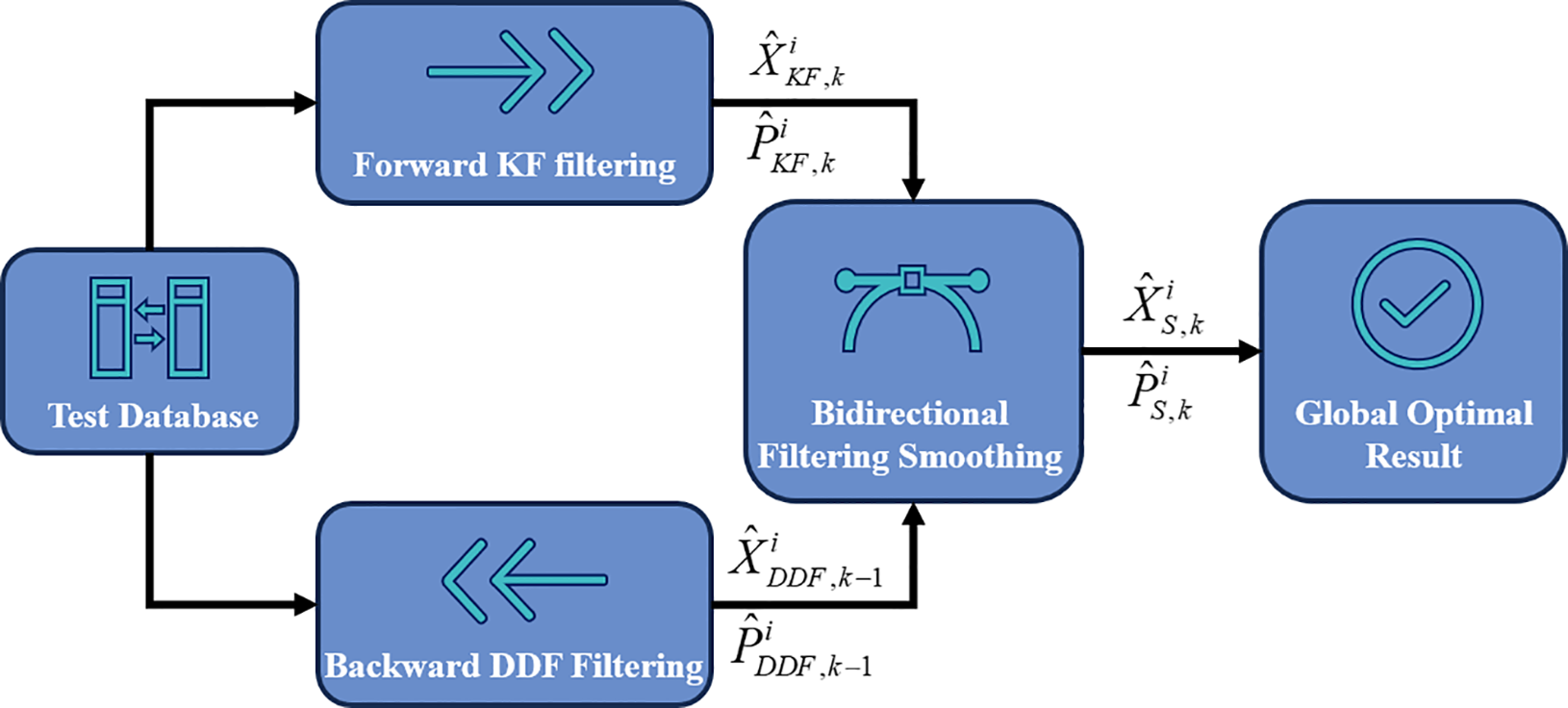
Figure 2. Data smooth processing flow.

The mathematical model is as follows (Equations 35–37). The results of forward and backward filtering are jointly considered, and the global optimal estimates ${\widehat{X}}_{S,k}^i$ and ${\widehat{P}}_{S,k}^i$ are obtained through data fusion. The calculation formulae are as follows (Chen et al., 2021):

$\begin{array}{ll}\{\begin{array}{l}{E}_{KF,k}^i={({\widehat{P}}_{KF,k}^i)}^{-1}\hfill \\ E_{DDF,k-1}^i={({\widehat{P}}_{DDF,k-1}^i)}^{-1}\hfill \end{array}& (35)\end{array}$

$\begin{array}{ll}{E}_{S,k}^i={(E_{KF,k}^i+E_{DDF,k}^i)}^{-1}& (36)\end{array}$

$\begin{array}{ll}{\widehat{X}}_{S,k}^i=E_{S,k}^i(E_{KF,k}^i{\widehat{X}}_{KF,k}^i+E_{DDF,k-1}^i{\widehat{X}}_{DDF,k-1}^i)& (37)\end{array}$

Finally, the updated global optimal solution is fed back into the carrier and pseudocode tracking loops.

3 Experiments and analysis

3.1 Experiment description

To validate the effectiveness of the loop tracking method proposed in this study and quantitatively evaluate and analyze its performance, we designed and conducted a series of navigation experiments in real-world scenarios. The primary objective of these experiments was to verify the superiority of the proposed method in improving the signal tracking accuracy, enhancing the anti-interference capability, and increasing the system robustness. Additionally, by comparing its performance with different methods, the experiments aimed to further quantify the improvements achieved. The data acquisition and processing platform used in the experiment is shown in Figure 3.

Figure 3

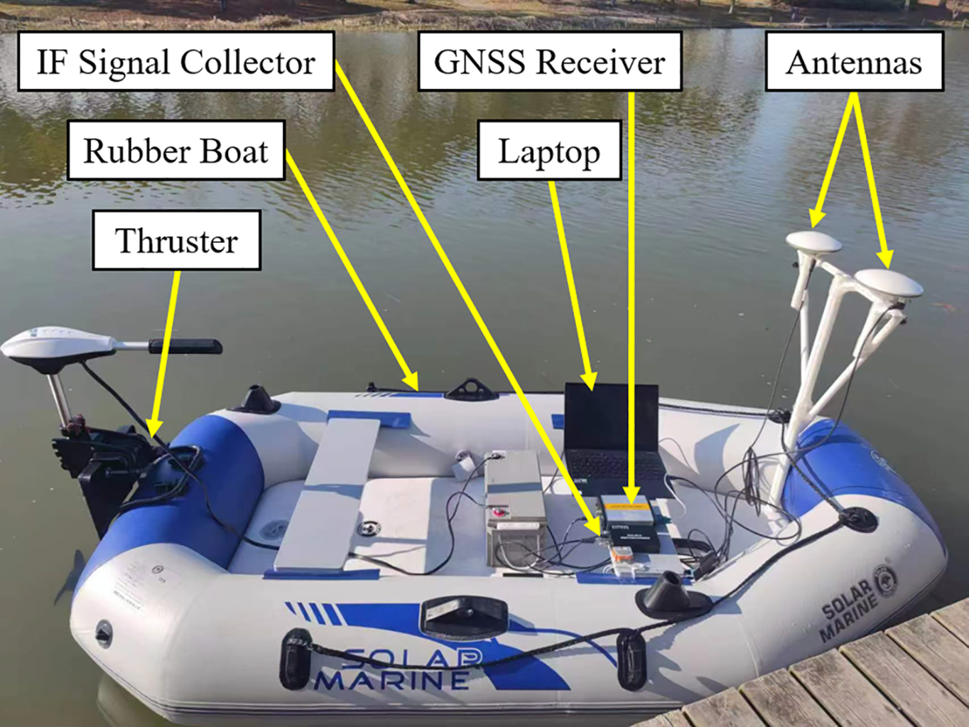
Figure 3. Shipborne experimental platform.

In the experiment, we selected a rubber boat as the platform to carry the experimental equipment, simulating the motion and operational scenarios of a shipborne platform under real-world conditions. The experimental equipment included a specialized receiver for collecting GPS intermediate frequency (IF) signals, high-precision navigation receiver module for real-time measurement and recording of positioning information, two full-band measurement antennas, and laptop for data storage and processing. This setup not only meets the requirements of the experiment for signal acquisition, but also provides comprehensive support for subsequent data analysis and processing, ensuring the reliability and accuracy of the experimental results. The performance parameters of the equipment are presented in the Table 1.

Table 1

Table 1. Devices parameters.

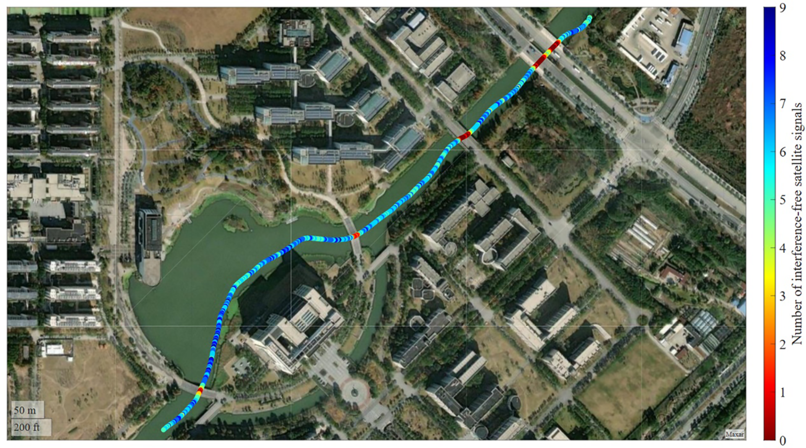
In the experiment, we selected a river with a moderate width and a complex environment to simulate the operating status of ships in actual navigation. There are many bridges above the river in the experimental route. These bridges not only serve as a reproduction of the actual scene but also play the role of satellite signal obstructions in the experiment, which can effectively simulate the obstruction and multipath effects in the signal propagation path. By conducting experiments in such an environment, we can comprehensively test the navigation accuracy and robustness of different algorithm systems in complex environments. In addition, the experiment simulated the changes in signal quality under different degrees of obstruction by blocking the signal with bridges of different widths to evaluate the adaptability and performance of each system under harsh signal conditions, thereby providing valuable reference data for practical applications. The experimental trajectory is shown in Figure 4. Specific scenarios of bridge obstructions are shown in Figures 5A-D.

Figure 4

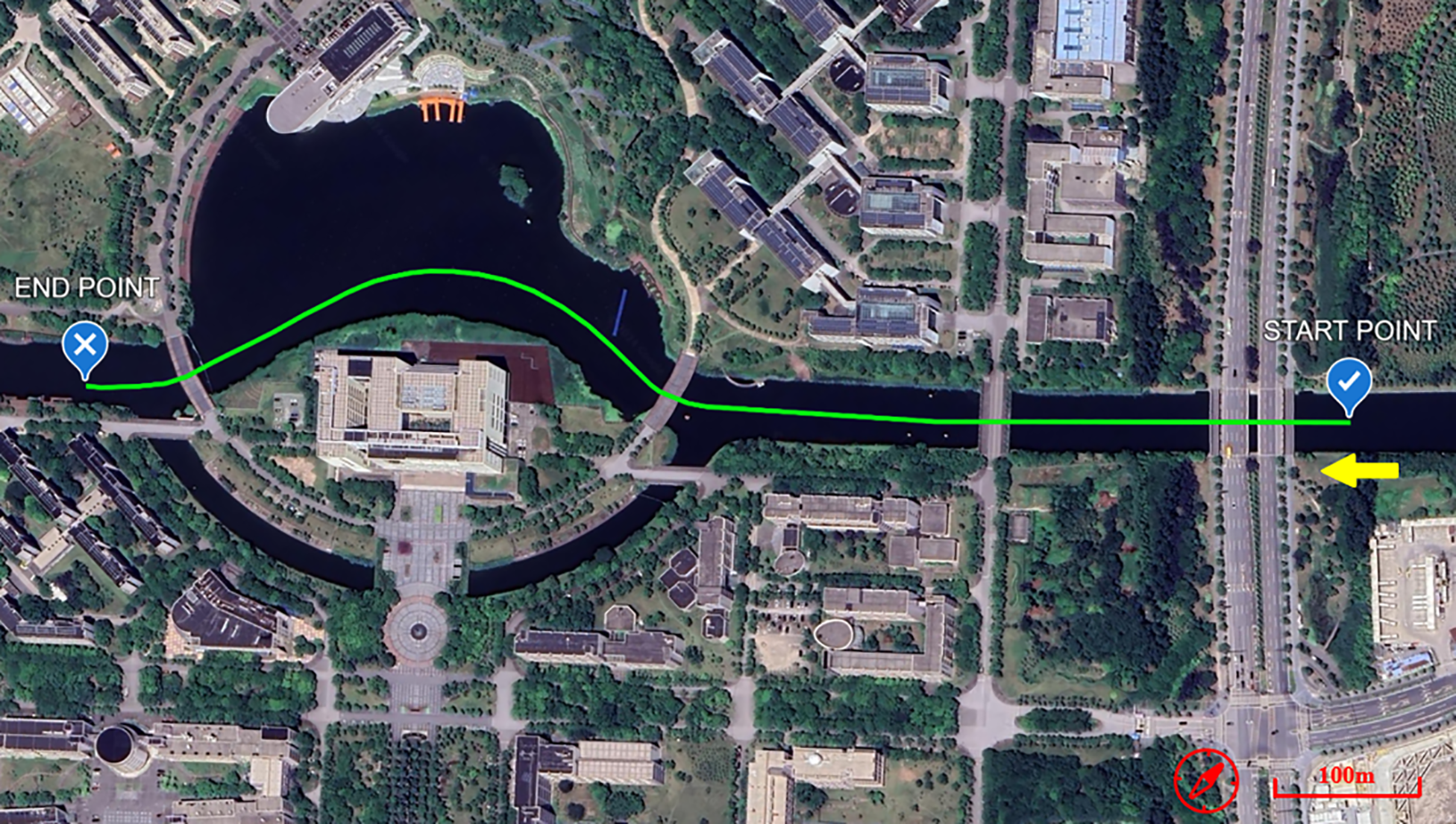
Figure 4. Experimental trajectory.

Figure 5

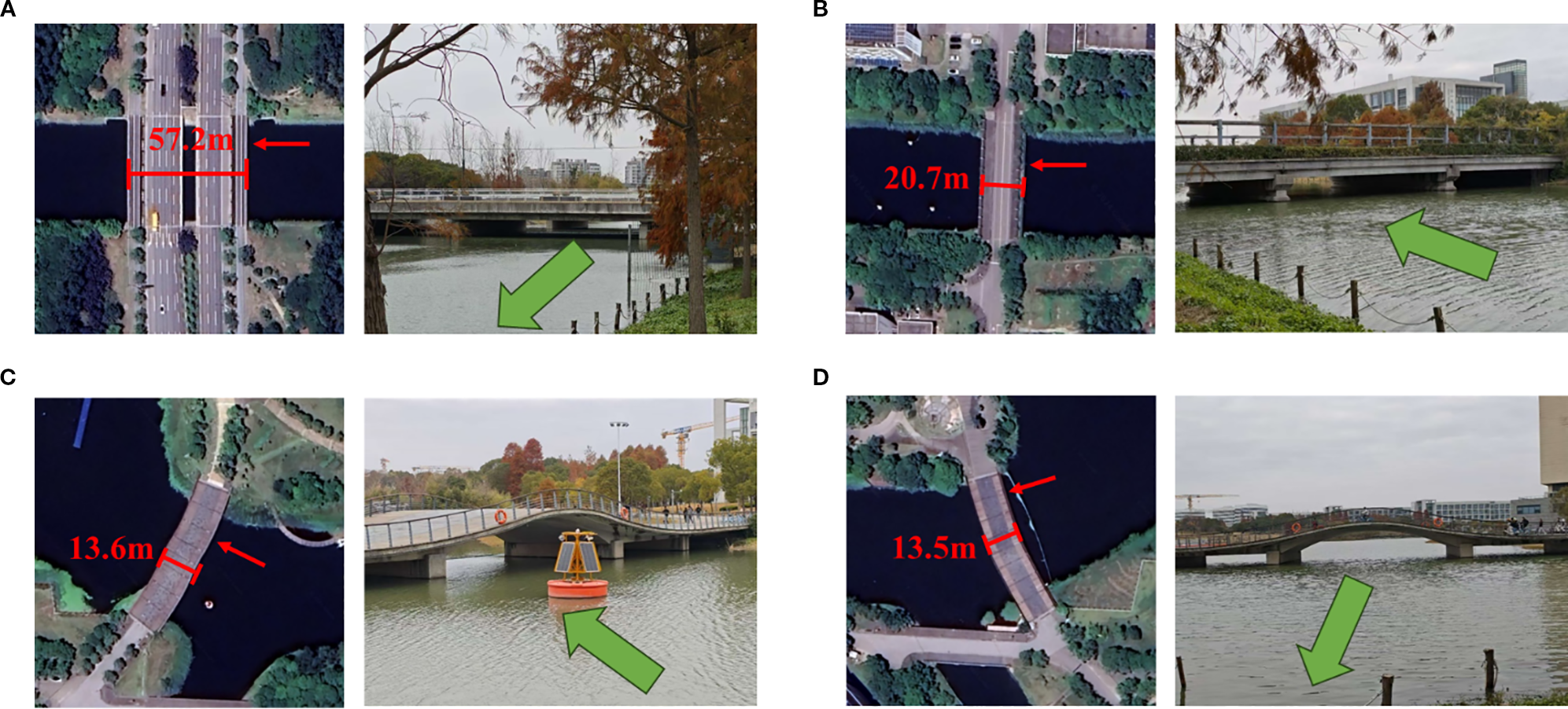
Figure 5. Four signal obstruction areas in the experimental scenario. (A) Bridge Obstruction Scenario 1. (B) Bridge Obstruction Scenario 2. (C) Bridge Obstruction Scenario 3. (D) Bridge Obstruction Scenario 4.

The total length of the experimental path was 900 meters. During the experiment, multiple bridges were crossed with widths of approximately 57.31 meters, 20.74 meters, 13.26 meters, and 12.65 meters, respectively. During the experimental phase, the rubber boat maintained a constant speed along the planned navigation trajectory. This setup was designed to continuously collect navigation data and to simulate the dynamic conditions of a shipborne platform during real-world operations. During the experiment, navigation data recorded by a high-precision Trimble BD-992 GNSS receiver was used as the reference trajectory. These data were compared with trajectories derived from different algorithms to evaluate the navigation accuracy and performance of each method. The entire experiment lasted for approximately 550 s.

3.2 The analysis of signal tracking loops

The number of interference-free satellite signals recorded during the experiment is shown in Figure 6. This figure illustrates the variation in the number of satellites captured by the receiver at different time points, allowing for intuitive observation of how signal occlusion and multipath effects impact satellite visibility and navigation accuracy. When there is a bridge obstruction, the number of interference-free satellite signals drops sharply, which leads to a rapid decrease in the accuracy of the navigation system, thereby affecting the reliability of the system.

Figure 6

Figure 6. Number of interference-free satellite signals.

In the initial stage of the experiment, six GPS satellites were successfully acquired based on the elevation angle and signal-to-noise ratio conditions, which served as the basis for the subsequent signal-loop tracking process. The satellite acquisition results are shown in Figure 7.

Figure 7

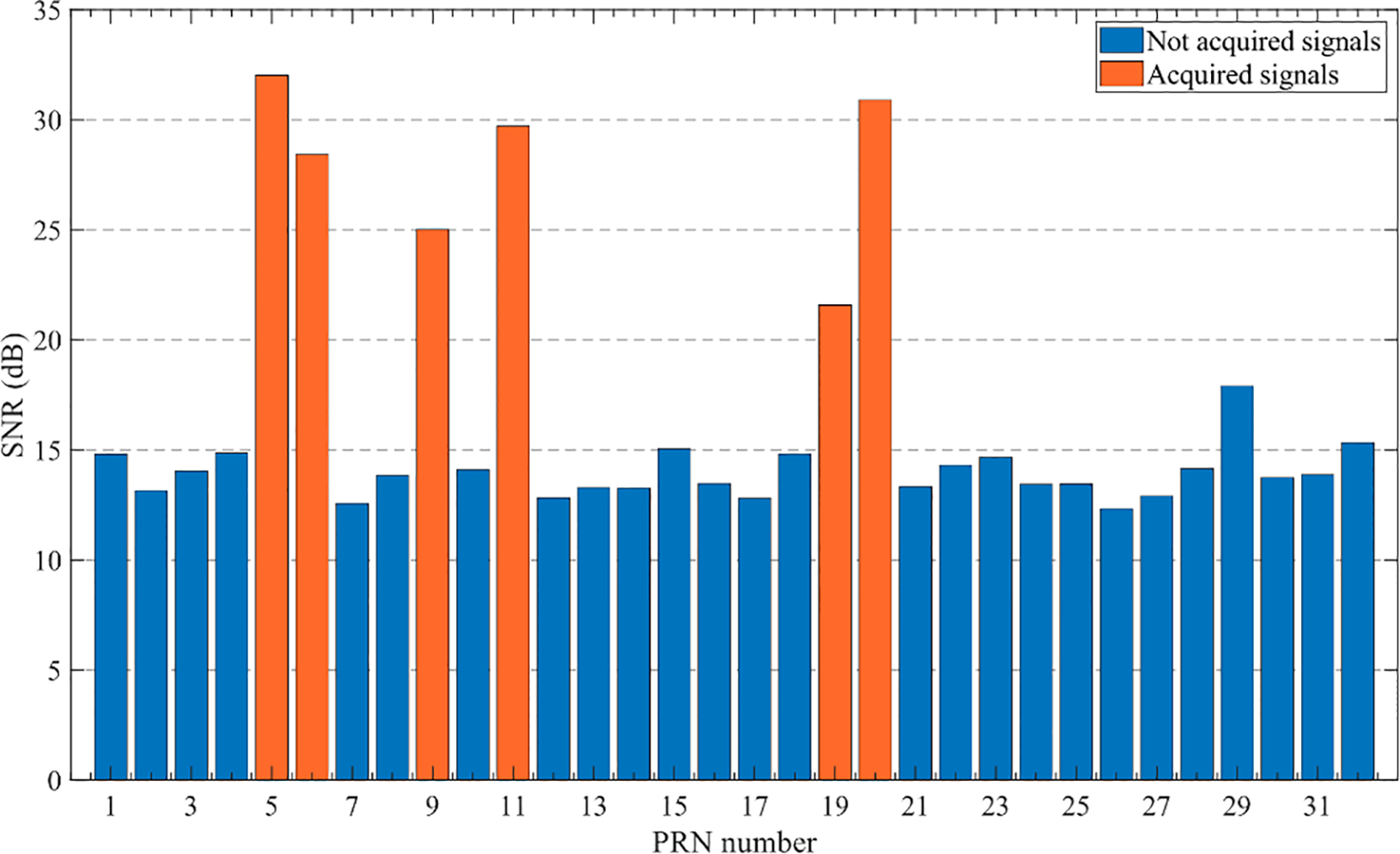
Figure 7. The acquisition result of satellite signals.

CNR is a direct parameter that measures the quality of the satellite signal received by the navigation receiver. By representing the ratio of the satellite signal’s strength to the noise density, CNR is an essential parameter for evaluating the reliability of the satellite navigation system and the performance of the signal-tracking loops. As shown in Figure 8, the CNR results obtained throughout the experiment illustrate the signal quality of the captured satellites. Under complex environmental conditions, variations in the CNR reveal the effects of signal blockage, multipath interference, and electromagnetic disturbances, providing valuable insights for optimizing navigation systems. Figure 8 shows the dynamic changes in signal quality during the entire experiment.

Figure 8

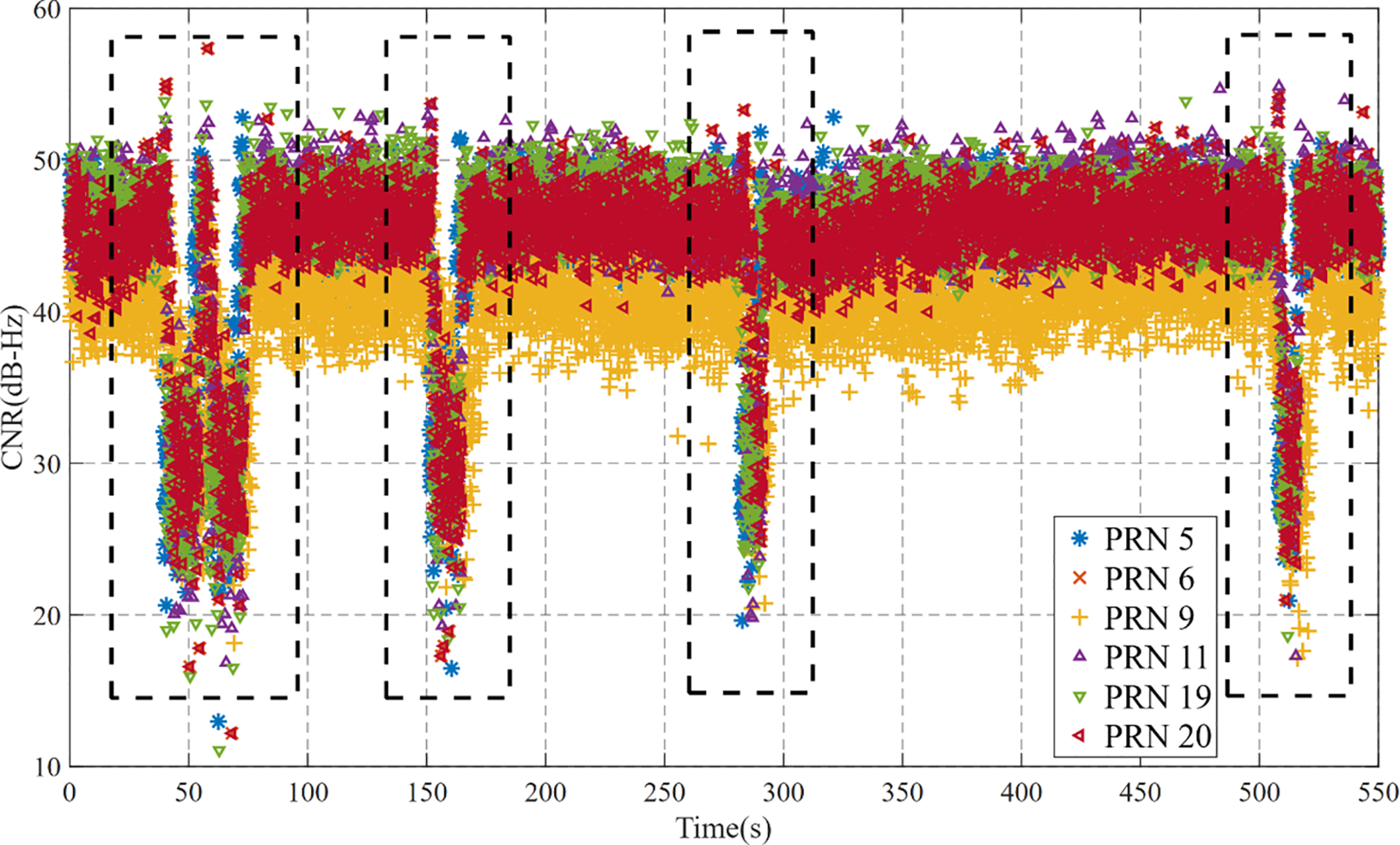
Figure 8. The result of CNR during the experiment.

As shown in Figure 8, it is evident that when the rubber boat passes under bridges with signal obstruction, the CNR of the satellite signals quickly drop below to 30 dB-Hz. This indicates that the signal quality received by the receiver deteriorates significantly owing to the severe obstruction. Under such conditions, the navigation system may face difficulties in tracking and may even risk losing the signal.

To further analyze the impact of environmental obstructions and other factors on the pseudocode and carrier signals, as well as their relationship with navigation accuracy, Figure 9 illustrates the loop tracking performance of the PRN6 satellite during the experiment. The single tracking conditions of the other satellites are similar and are not detailed here. The comparison includes the traditional STL, traditional VTL, Kalman filter-based VTL algorithm, and method proposed in this study to evaluate the performance of each method.

Figure 9

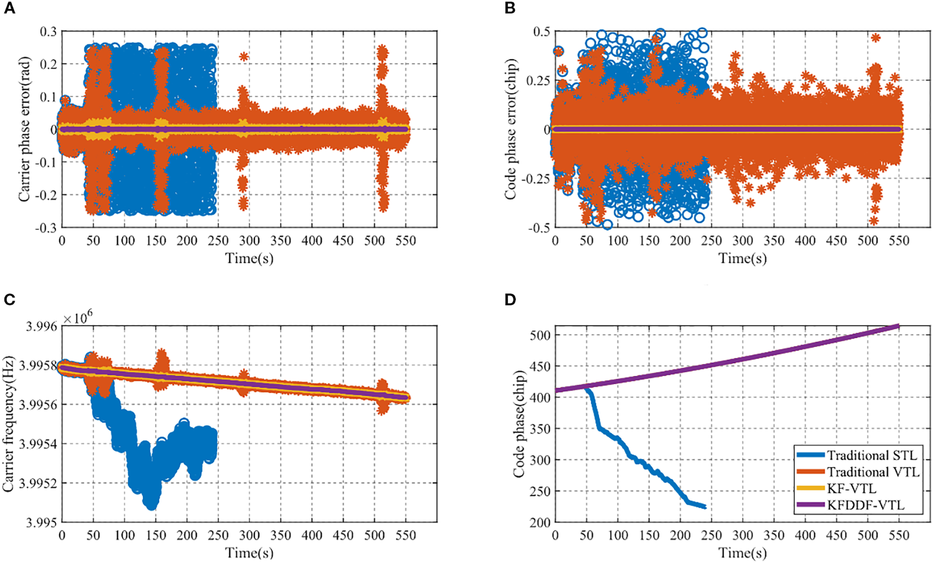
Figure 9. The signal loop tracking results of PRN6. (A) Carrier phase error of PRN 6, (B) Code phase error of PRN 6, (C) Carrier tracking frequency of PRN 6, (D) Code phase tracking of PRN 6.

Figure 9 illustrates the signal loop-tracking performance of the PRN6 GPS satellite. As shown in the figure, the tracking accuracy of the carrier and code in the traditional STL and VTL algorithms are significantly affected under signal interference conditions. In particular, the traditional STL method experiences a gradual divergence in the carrier and code phase errors when subjected to severe signal obstruction. This accumulation of errors leads to frequency tracking deviations, ultimately causing a signal loss of lock at 241 s.

This observation highlights the limitations of the STL method in handling signal interference in complex environments, whereas vector tracking methods demonstrate certain advantages under challenging and interference-prone conditions. Because of the loss-of-lock phenomenon observed with the STL, subsequent experimental analysis excludes discussions on the STL signal loop performance.

In addition, throughout the experiment, the method proposed in this paper demonstrated higher signal tracking accuracy and stronger signal loop stability when facing interference compared with other methods. When encountering a signal blockage or complex environmental interference, traditional methods often experience a sharp decline in tracking accuracy or even signal loss. Although the VTL method based on the Kalman filter (KF-VTL) has significantly improved performance, it still has a significant decline in accuracy when the signal is blocked. In contrast, the proposed method can consistently maintain a high tracking accuracy and ensure the stability of the signal loop, even under significant interference. This provides a solid foundation for achieving stable high-precision navigation.

3.3 Positioning optimization results

The shipborne experimental navigation and positioning results are shown in Figure 10. In this experiment, the high-precision GNSS navigation receiver Trimble BD992 was used to generate the reference trajectory, which is represented by the black line in the figure. To evaluate the positioning performance of different methods comprehensively, the experiment compared the results of the traditional STL, traditional VTL, Kalman Filter based VTL method (KF-VTL), and KF-DDF-based VTL method proposed in this study. From the figure, it can be intuitively observed that the performance of the different methods in terms of navigation accuracy shows significant differences. The traditional STL and VTL methods are easily affected by signal interference and blockages in complex environments, resulting in deviations and accuracy divergence in the positioning results. In particular, the traditional STL method experienced signal loss during the experiment, resulting in an inability to provide positioning results. Although the KF-based VTL method improves performance, it still shows a noticeable drop in accuracy under signal blockage conditions. In contrast, the KF-DDF-based VTL method proposed in this study demonstrated significant advantages by consistently providing stable and high-accuracy navigation and positioning results throughout the experiment, effectively overcoming the negative impacts caused by signal interference and blockage.

Figure 10

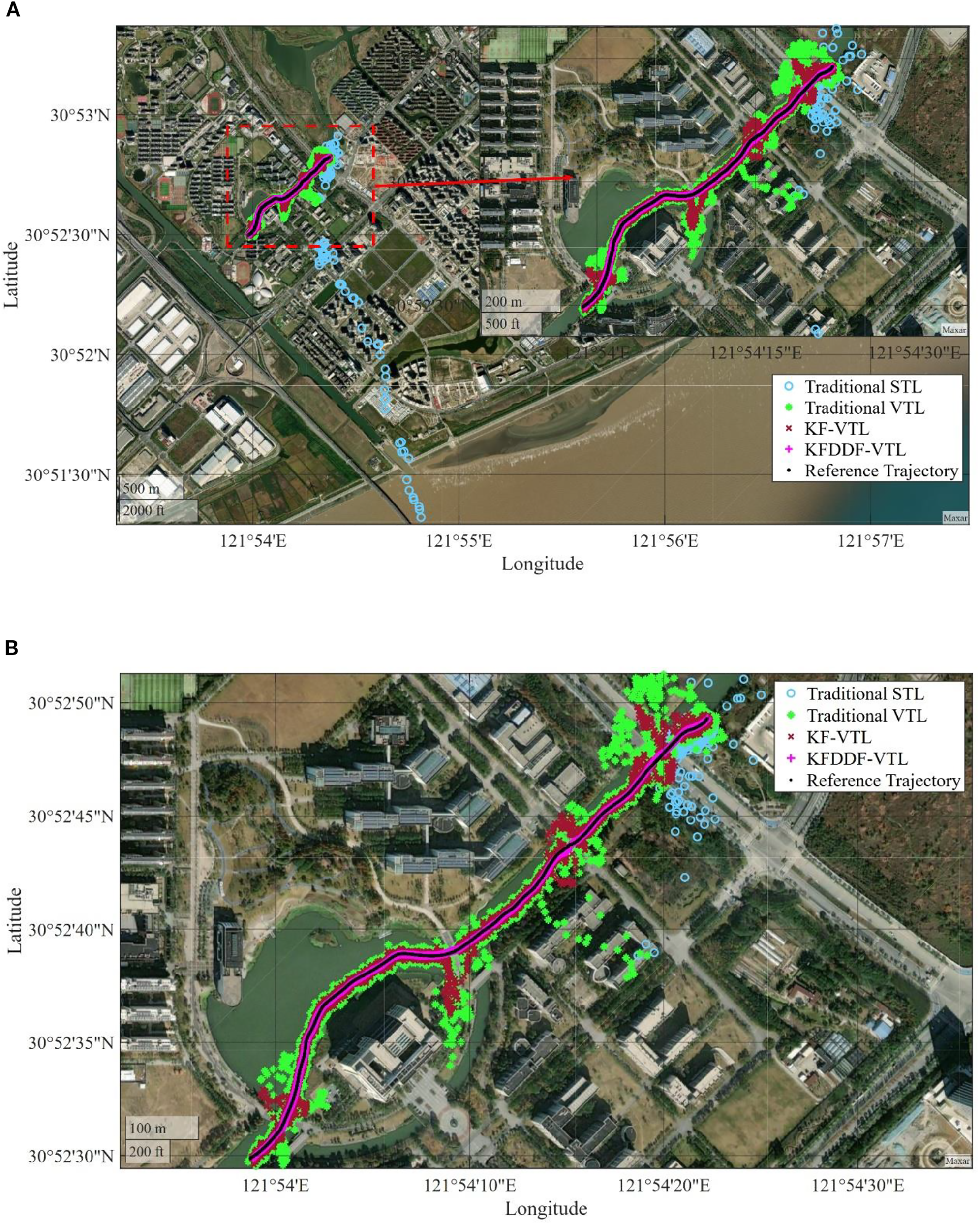
Figure 10. Comparison of position results with different methods. (A) Overall diagram, (B) Zoomed-in diagram.

The velocity results of the different methods under signal obstruction conditions for the experimental rubber boat are shown in Figure 11. It can be observed from the figure that at 47 s in the experiment, the rubber boat passed under a bridge where the satellite signals experienced significant obstruction and interference, causing a rapid decline in the navigation solution performance of the traditional STL method. Starting at 50 s, the velocity results began to diverge, exhibiting a noticeable instability. This divergence indicates that the signal-tracking loop fails to maintain accurate tracking under obstructed and interfered conditions. Furthermore, owing to continuous signal obstruction, the signal tracking loop of the traditional STL method completely loosed lock at 241 s, making it incapable of continuing to track satellite signals. This results in the failure of the navigation system, and the speed solution outcomes lose all reference values.

Figure 11

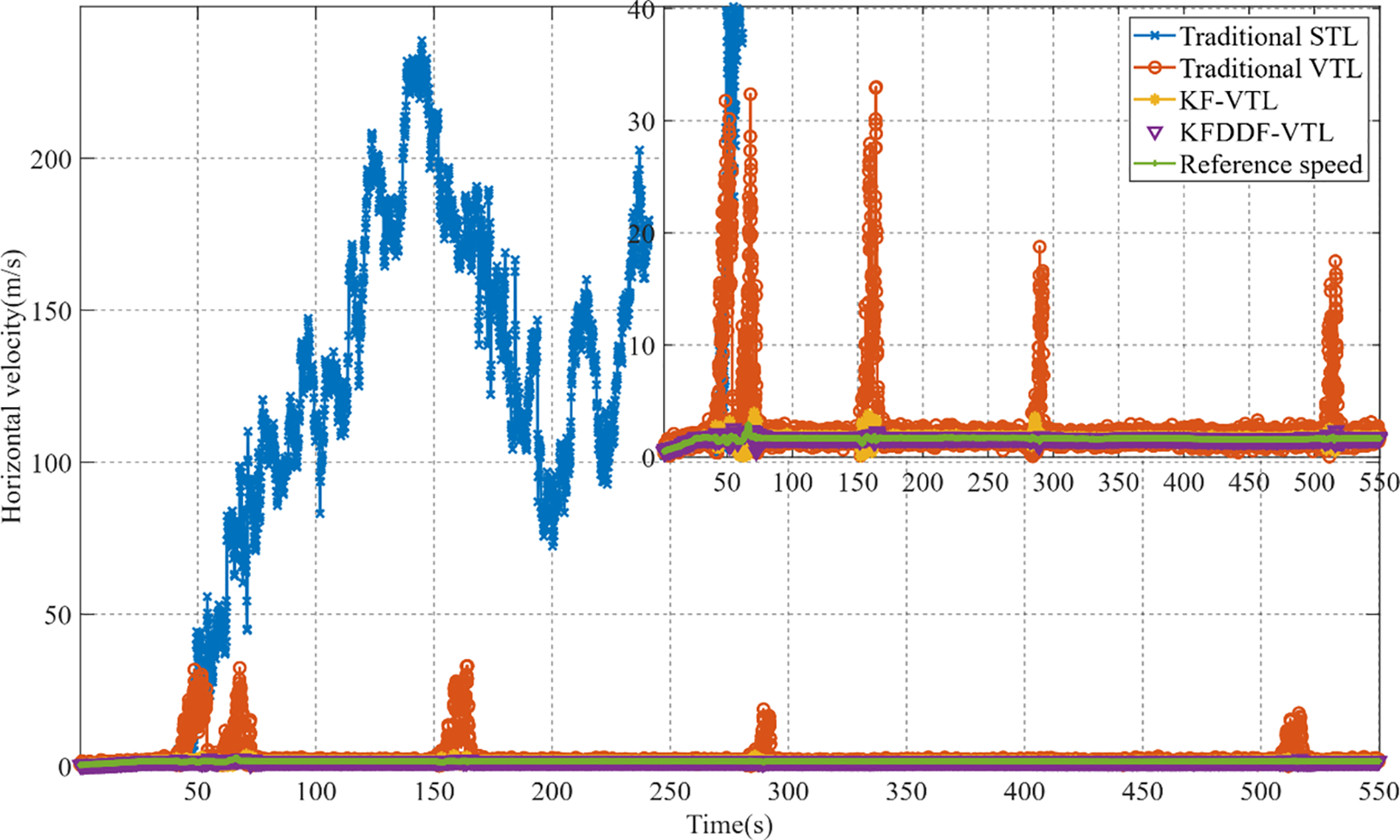
Figure 11. Comparison of velocity results with different methods.

The traditional VTL method exhibits significant velocity errors in weak signal environments, particularly when signals are obstructed or interfered with, resulting in noticeable instability in the velocity outcomes. The KF-based VTL method improves the velocity measurement accuracy compared with traditional methods and mitigates the impact of signal interference. However, under prolonged weak signals or severe obstructions, the velocity results still showed a decline in accuracy. In contrast, the proposed KF-DDF based VTL method demonstrates the best velocity calculation accuracy among all the compared methods. Even in weak signals or obstructed environments, this method effectively reduces the impact of signal interference on the navigation system, providing more stable and accurate velocity results. This highlights the excellent system robustness and ability to adapt to complex environments, further validating the superior performance of the proposed method in high-precision navigation applications.

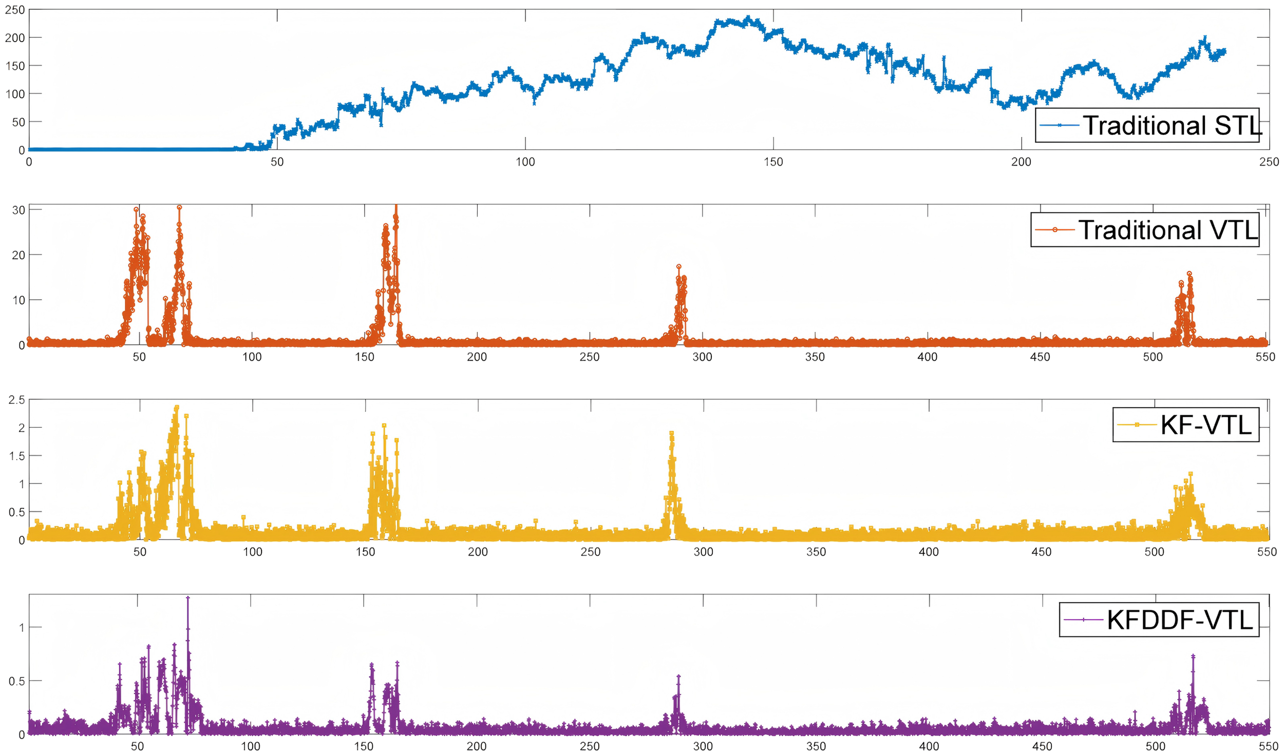
The position and velocity errors are presented in Figures 12, 13, respectively. From the results, it can be observed that the traditional STL is severely affected in signal blockage environments, leading to a signal loss of lock. This causes a significant increase in the position and velocity errors, far exceeding the normal error range of the tracking loop. At this point, the navigation system based on traditional STL can no longer function properly.

Figure 12

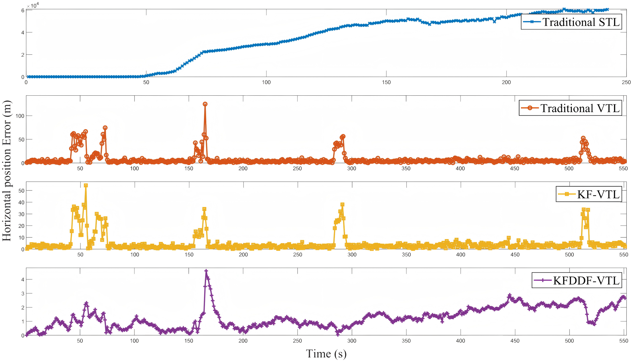
Figure 12. Horizontal position errors.

Figure 13

Figure 13. Horizontal velocity errors.

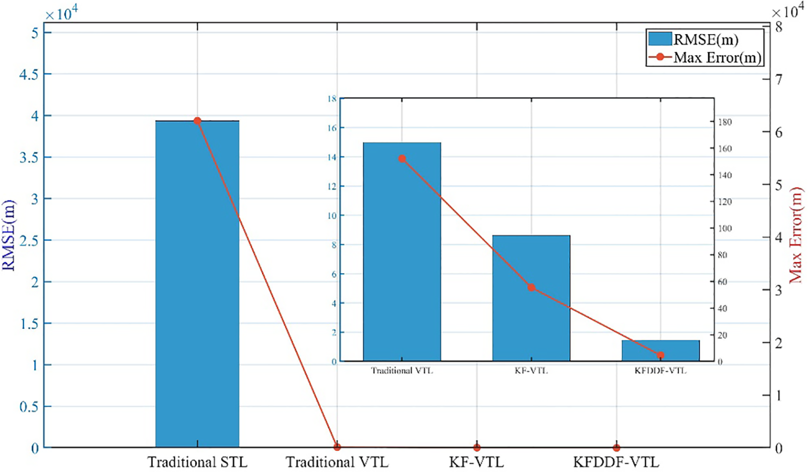
Compared to traditional VTL and KF-VTL, the proposed KF-DDF based VTL method demonstrates significant advantages in terms of position and velocity accuracy. Specifically, the proposed method improves the position accuracy by 90.33% compared to the traditional VTL method and by 83.20% compared to the KF-based VTL method. In terms of velocity accuracy, it achieves an improvement of 96.83% over the traditional VTL method and 60.0% over the KF-based VTL method. The navigation error results of the four comparison methods are presented in Table 2; Figures 14, 15. These results indicate that the proposed method can effectively overcome the adverse effects of signal blockages and interference in complex environments, thereby significantly improving the accuracy of the navigation system and demonstrating higher robustness and stability.

Table 2

Table 2. Results of four different methods.

Figure 14

Figure 14. Horizontal position error bar chart.

Figure 15

Figure 15. Horizontal velocity error bar chart.

3.4 Positioning experiment under ocean navigation

In the marine navigation experiment, a satellite signal reception scenario from an ocean-going vessel during its voyage was selected as the test subject, with 600 consecutive seconds of data extracted for analysis and evaluation. Through practical marine environment experiments, the performance of the proposed method in shipborne navigation applications can be directly and effectively evaluated. Similarly, the experiment compared several commonly used navigation signal tracking methods, including the traditional scalar tracking (STL) method, the traditional vector tracking (VTL) method, the FKF-VTL method, and the proposed FK-DDF based VTL method. The experimental path is shown in Figure 16.

Figure 16

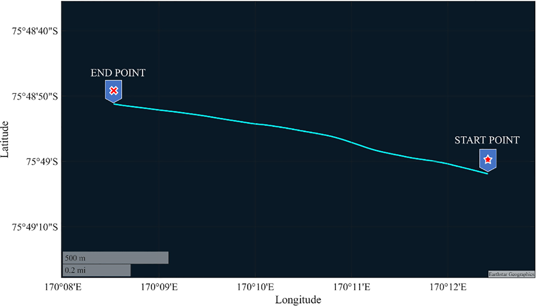
Figure 16. Experimental trajectory.

The acquisition results of GPS navigation satellites in this experiment are shown in Figure 17, with signals from a total of 8 satellites successfully captured. The signal loop tracking conditions of satellites PRN6 and PRN11 were selected for analysis, as shown in Figures 18, 19. It is evident that the satellite signals maintained stable reception throughout the entire experiment, and the system rapidly achieved signal loop tracking shortly after the experiment commenced. In addition to traditional scalar tracking methods, vector tracking schemes also demonstrated superior signal tracking performance. Through this comparative experiment, the navigation accuracy performance of different methods can be further evaluated under both ideal satellite signal reception conditions and real-world marine signal environments.

Figure 17

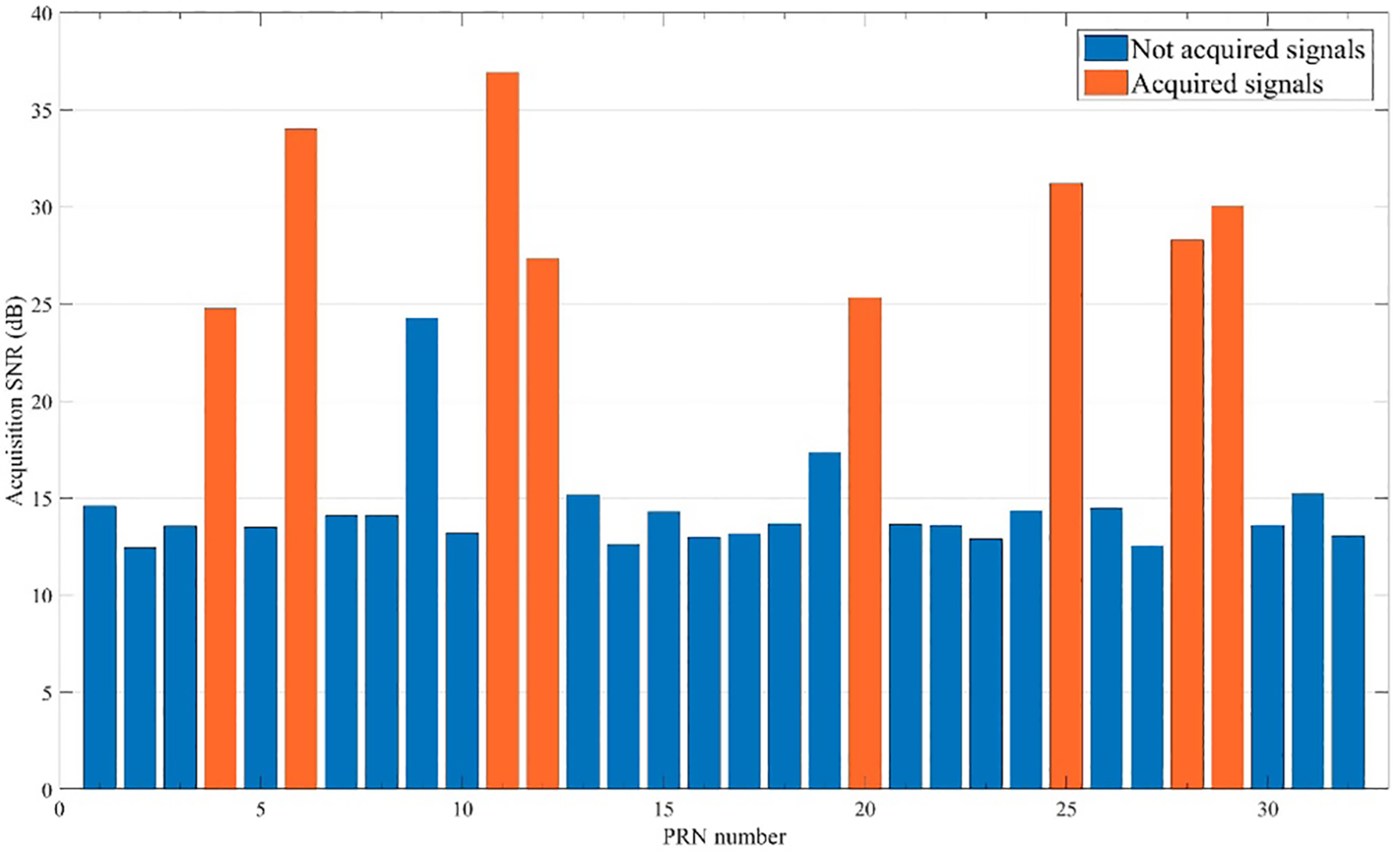
Figure 17. The acquisition result of satellite signals.

Figure 18

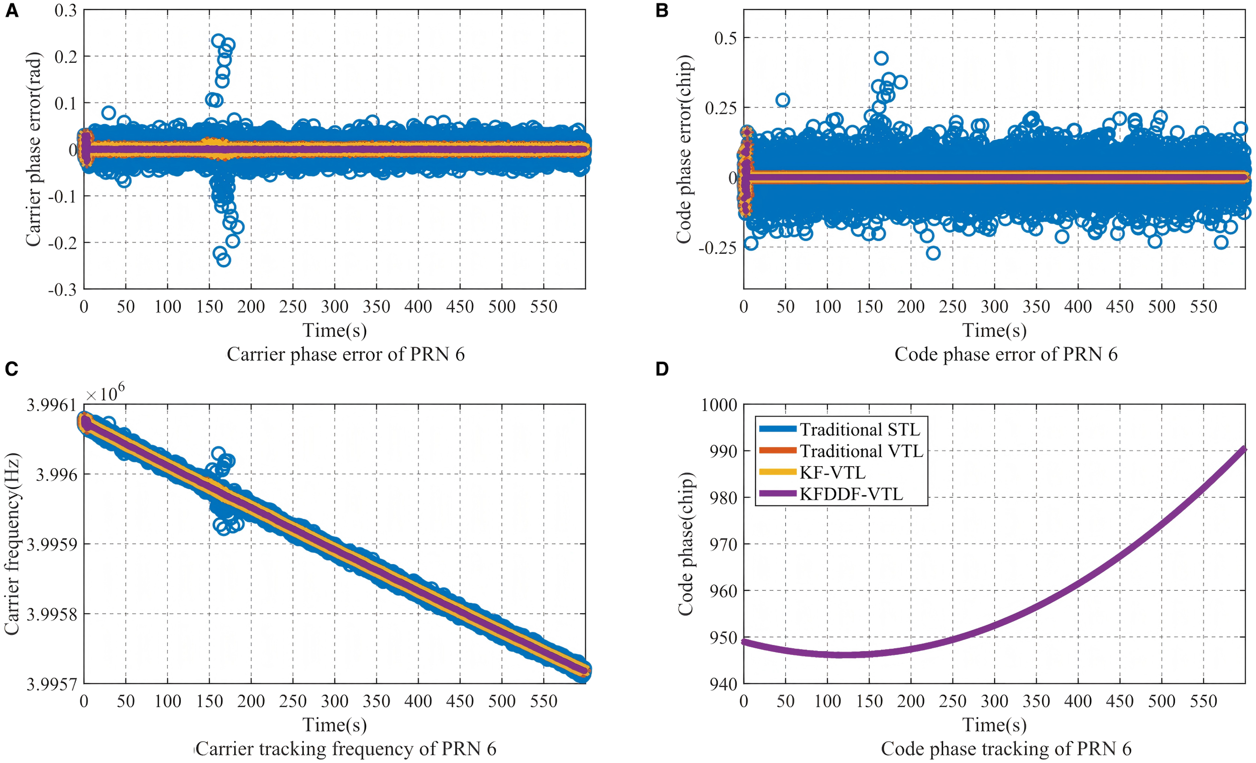
Figure 18. The signal loop tracking results of PRN 6. (A) Carrier phase error of PRN 6, (B) Code phase error of PRN 6, (C) Carrier tracking frequency of PRN 6, (D) Code phase tracking of PRN 6.

Figure 19

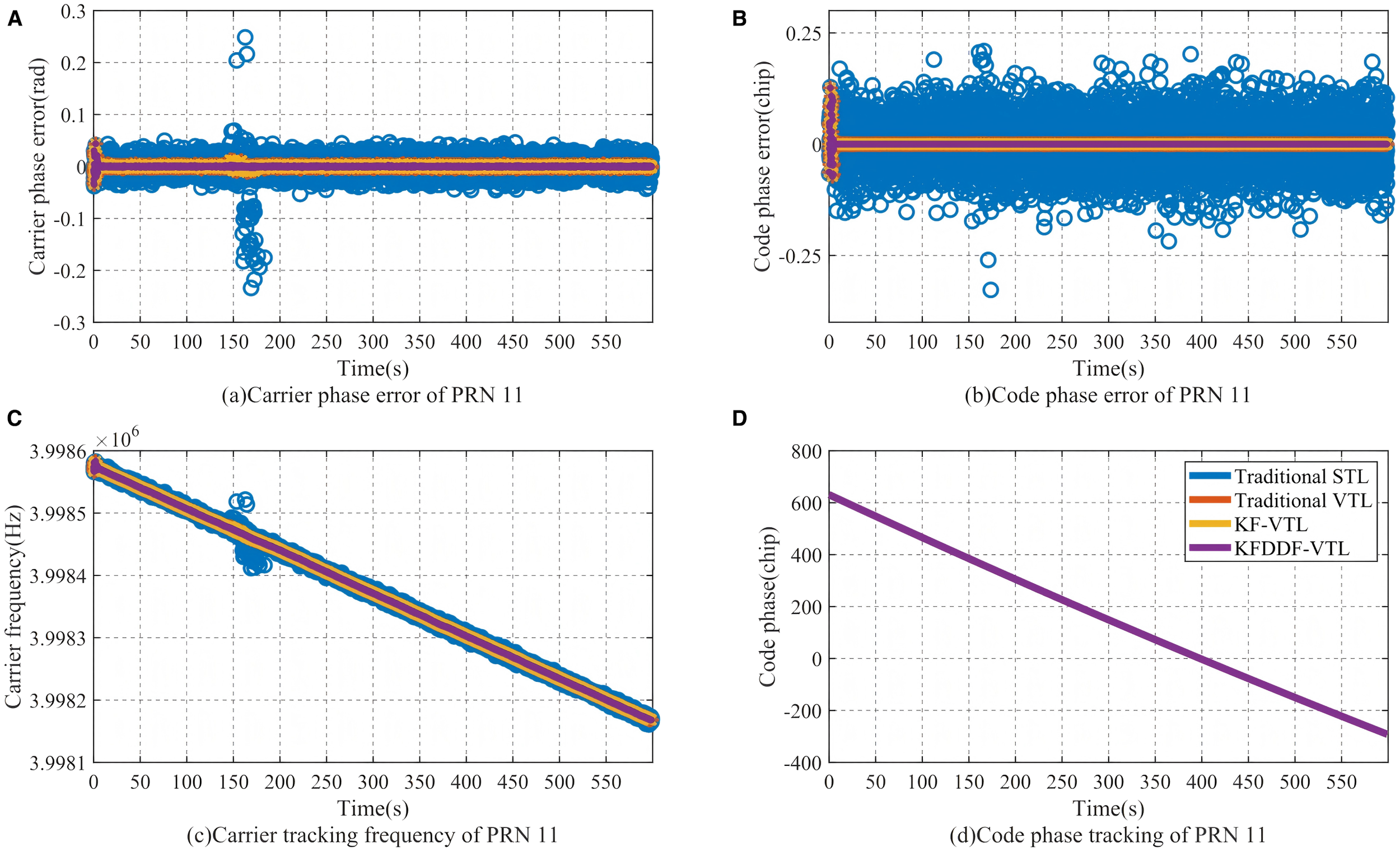
Figure 19. The signal loop tracking results of PRN 11. (A) Carrier phase error of PRN 11, (B) Code phase error of PRN 11, (C) Carrier tracking frequency of PRN 11, (D) Code phase tracking of PRN 11.

As illustrated in Figures 20, 21, the comparative analysis of positioning and velocity results demonstrates the performance of different navigation methods, with corresponding error metrics calculated and tabulated in Table 3. The error bar chart is plotted as shown in Figures 22, 23. The results clearly indicate that under favorable signal conditions, the proposed method maintains consistently higher navigation accuracy compared to the other three methods.

Figure 20

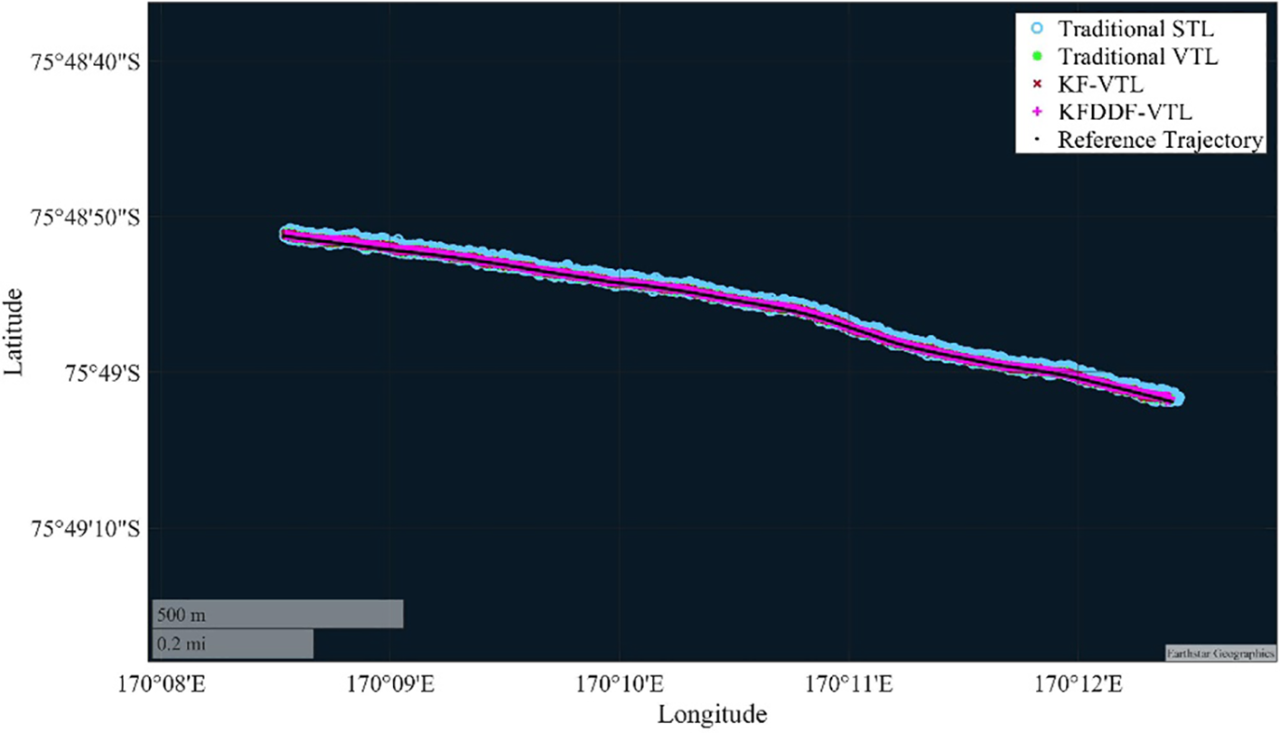
Figure 20. Comparison of position results with different methods.

Figure 21

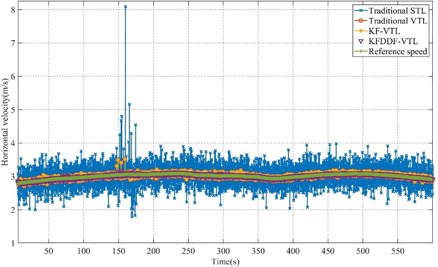
Figure 21. Comparison of velocity results with different methods.

Table 3

Table 3. Results of four different methods.

Figure 22

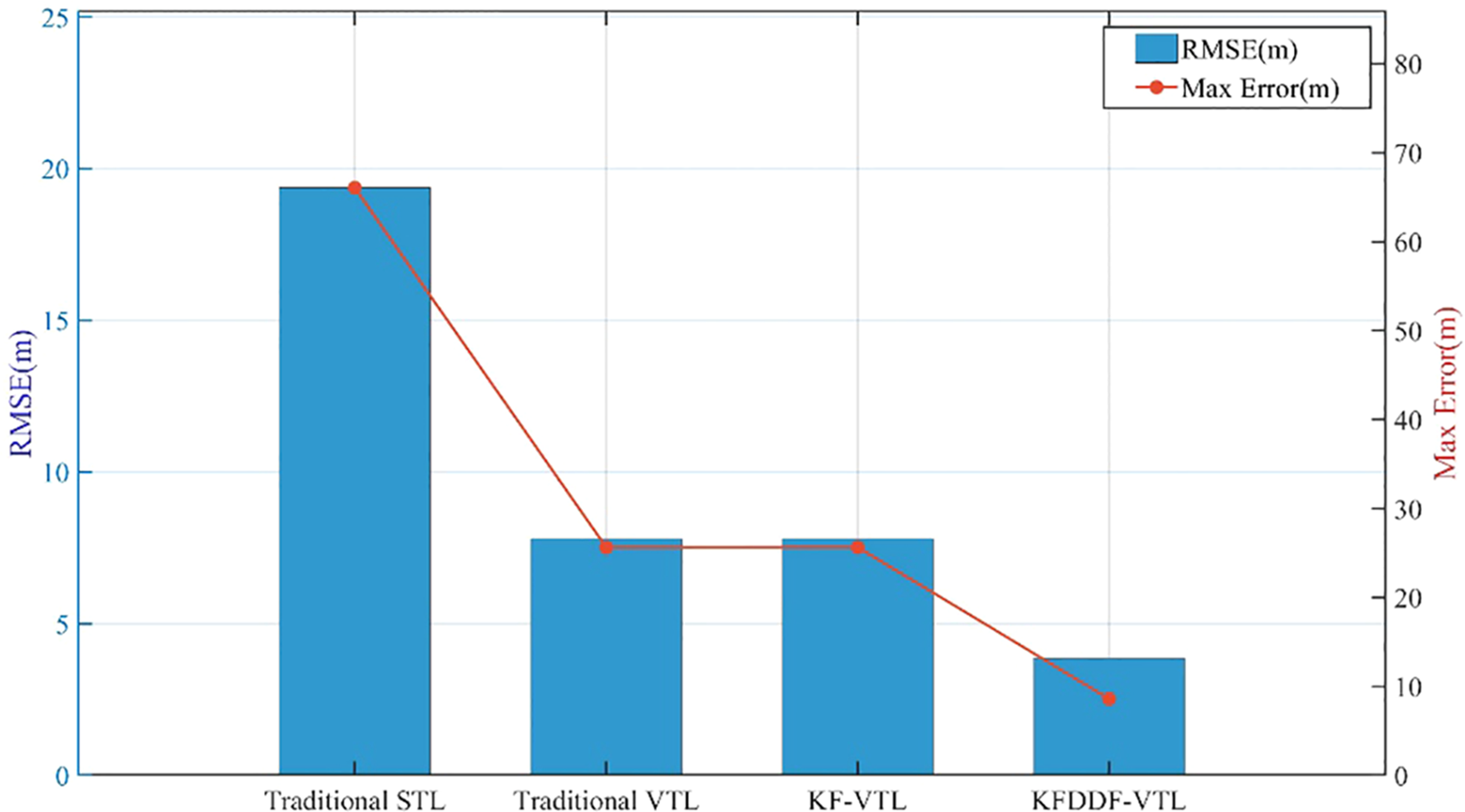
Figure 22. Horizontal position error bar chart.

Figure 23

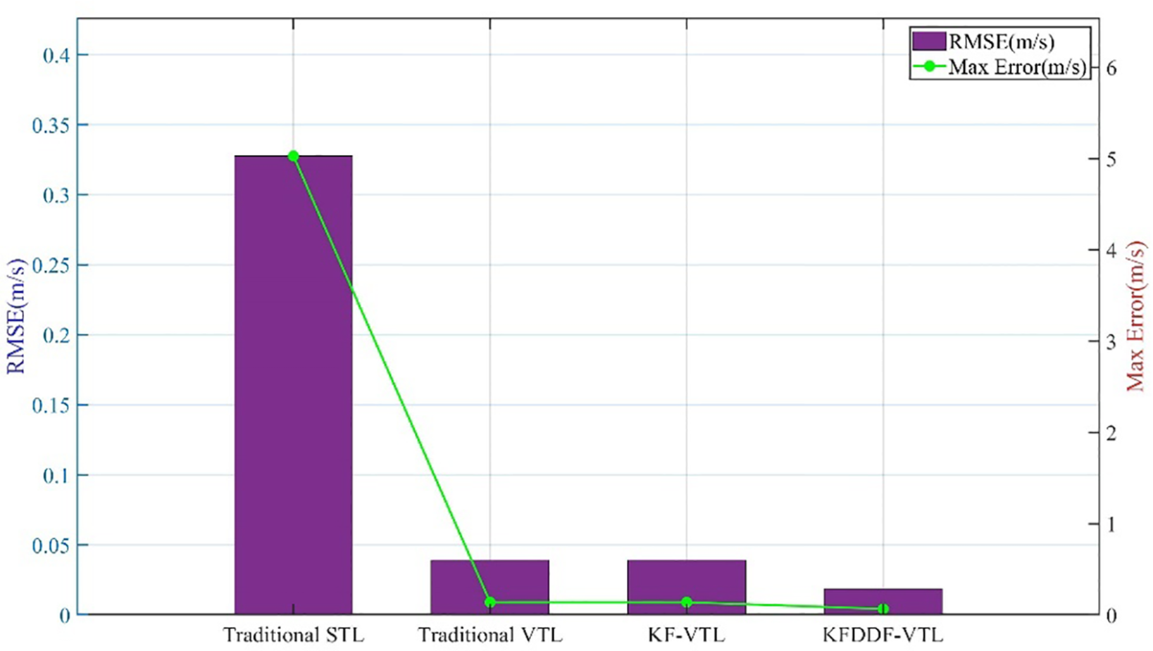
Figure 23. Horizontal velocity error bar chart.

4 Conclusion and discussion

In this study, an improved bidirectional filter VTL method based on the fusion of Kalman filter and Divided Difference filter is proposed to solve the problem of signal interference and occlusion in satellite navigation systems in complex environments. The loop filter mathematical model of the proposed method is derived in detail, and the effectiveness of the proposed method is verified by actual ship experiments. Compared with the navigation accuracy of traditional VTL and KF-based VTL, the proposed method improved the horizontal position accuracy by 90.33% compared with traditional VTL and 83.20%, KF-based VTL. The horizontal velocity accuracy was improved by 96.83% and 60.0%, respectively. Moreover, this paper conducted an experiment on shipborne navigation systems in a marine environment, which fully validated the effectiveness of the proposed method.

In addition, the KF-DDF based VTL method effectively maintained the stability of the signal-tracking loop in weak signal and interference environments. The experimental results showed that this method significantly improved the accuracy, robustness, and anti-interference capability of navigation systems, thereby providing reliable technical support for the development of high-precision shipborne navigation systems in complex sailing environments.

Data availability statement

The raw data supporting the conclusions of this article will be made available by the authors, without undue reservation.

Author contributions

LW: Conceptualization, Data curation, Formal Analysis, Funding acquisition, Methodology, Software, Validation, Visualization, Writing – original draft, Writing – review & editing. WL: Conceptualization, Data curation, Formal Analysis, Funding acquisition, Project administration, Resources, Supervision, Writing – original draft. YH: Conceptualization, Investigation, Methodology, Supervision, Writing – original draft. SW: Project administration, Validation, Visualization, Writing – original draft.

Funding

The author(s) declare that financial support was received for the research and/or publication of this article. This work was sponsored by the National Natural Science Foundation of China (52071199).

Conflict of interest

The authors declare that the research was conducted in the absence of any commercial or financial relationships that could be construed as a potential conflict of interest.

Generative AI statement

The author(s) declare that no Generative AI was used in the creation of this manuscript.

Any alternative text (alt text) provided alongside figures in this article has been generated by Frontiers with the support of artificial intelligence and reasonable efforts have been made to ensure accuracy, including review by the authors wherever possible. If you identify any issues, please contact us.

Publisher’s note

All claims expressed in this article are solely those of the authors and do not necessarily represent those of their affiliated organizations, or those of the publisher, the editors and the reviewers. Any product that may be evaluated in this article, or claim that may be made by its manufacturer, is not guaranteed or endorsed by the publisher.

References

Abedi A. A. and Mosavi M. R. (2022). Low Computational-Complexity vector tracking for Low-Cost GNSS receivers. Measurement 195. doi: 10.1016/j.measurement.2022.111171

Crossref Full Text | Google Scholar

Chen D., Wen J., Dai H., Xi M., Xiao S., and Yang J. (2024a). Enhancing transportation management in marine internet of vessels: A 5G broadcasting-centric framework leveraging federated learning. IEEE Trans. Broadcast. 70, 1091–11035. doi: 10.1109/tbc.2024.3394289

Crossref Full Text | Google Scholar

Chen D., Wen J., Xi M., Xiao S., Yang J., and Ieee (2024b). “Unmanned aerial vehicle path planning based on improved DDQN algorithm,” in 19th IEEE International Symposium on Broadband Multimedia Systems and Broadcasting (BMSB), Toronto, CANADA. pp. 1–6. doi: 10.1109/BMSB62888.2024.10608279

Crossref Full Text | Google Scholar

Chen D., Xi M., Wen J., He J., Dai H., and Li W. (2024c). Path planning of autonomous underwater vehicle for data collection of the internet of everything. Digital. Commun. Netw. doi: 10.1016/j.dcan.2024.10.004

Crossref Full Text | Google Scholar

Chen G., Liu Z., Yu G., and Liang J. (2021). A new view of multisensor data fusion: research on generalized fusion. Math. Prob. Eng. 2021 (1), 5471242. doi: 10.1155/2021/5471242

Crossref Full Text | Google Scholar

Farhad M. A., Mosavi M. R., and Abedi A. A. (2021). Fully adaptive smart vector tracking of weak GPS signals. Arabian. J. Sci Eng. 46, 1383–1393. doi: 10.1007/s13369-020-05172-4

Crossref Full Text | Google Scholar

Gao N., Chen X., Yan Z., and Jiao Z. (2024). Performance enhancement and evaluation of a vector tracking receiver using adaptive tracking loops. Remote Sens. 16. doi: 10.3390/rs16111836

Crossref Full Text | Google Scholar

Han Z., Liu D., Wei Z., Xu Y., and Li R. (2022). A Carrier phase tracking method for vector tracking loops. Gps. Sol. 26 (4), 111. doi: 10.1007/s10291-022-01302-7

Crossref Full Text | Google Scholar

Heyne M. C. (2007). Spacecraft precision entry navigation using an adaptive sigma point Kalman filter bank.

Google Scholar

Hsu L.-T., Jan S.-S., Groves P. D., and Kubo N. (2015). Multipath mitigation and NLOS detection using vector tracking in urban environments. Gps. Sol. 19, 249–2625. doi: 10.1007/s10291-014-0384-6

Crossref Full Text | Google Scholar

Jia Q., Luo Y., Xu B., Hsu L.-T., and Wu R. (2024). A robust vector tracking loop structure based on potential bias analysis. Chin. J. Aeronautics. 37, 405–4205. doi: 10.1016/j.cja.2023.11.013

Crossref Full Text | Google Scholar

Karlgaard C. D. and Schaub H. (2007). Huber-based divided difference filtering. J. Guidance. Control. Dynamics. 30, 885–891. doi: 10.2514/1.27968.

Crossref Full Text | Google Scholar

Karlgaard C. D. and Shen H. (2013). Robust state estimation using desensitized Divided Difference Filter. Isa. Trans. 52, 629–6375. doi: 10.1016/j.isatra.2013.04.009

PubMed Abstract | Crossref Full Text | Google Scholar

Lacarra E., Seoane T., Gonzalez R., Lopez M., and Navigat Inst (2019). “EGNOS performance navigation on board oceanographic Hesperides vessel,” in 32nd International Technical Meeting of the Satellite-Division-of-The-Institute-of-Navigation (ION GNSS), Miami, FL. pp. 1613–1624. doi: 10.33012/2019.16953

Crossref Full Text | Google Scholar

Lashley M., Bevly D. M., and Hung J. Y. (2009). Performance analysis of vector tracking algorithms for weak GPS signals in high dynamics. IEEE J. Select. Topics. Signal Process. 3, 661–6735. doi: 10.1109/jstsp.2009.2023341

Crossref Full Text | Google Scholar

Li J., Zou S., Gu B., and Fang J. (2019). Adaptive two-filter smoothing based on second-order divided difference filter for distributed position and orientation system. Sci China-Inform. Sci. 62(9):192204. doi: 10.1007/s11432-018-9765-y

Crossref Full Text | Google Scholar

Mu R. and Long T. (2021). Design and implementation of vector tracking loop for high-dynamic GNSS receiverDesign and implementation of vector tracking loop for high-dynamic GNSS receiver. Sensors. (Basel Switzerland). 21:5629. doi: 10.3390/s21165629

PubMed Abstract | Crossref Full Text | Google Scholar

Niu B., Zhuang X., Lin Z., and Zhang L. (2024). Navigation spoofing interference detection based on Transformer model. Adv. Space. Res. 74, 5156–51715. doi: 10.1016/j.asr.2024.07.016

Crossref Full Text | Google Scholar

Perera L. P. and Guedes Soares C. (2015). Collision risk detection and quantification in ship navigation with integrated bridge systems. Ocean. Eng. 109, 344–354. doi: 10.1016/j.oceaneng.2015.08.016

Crossref Full Text | Google Scholar

Reda A., Mekkawy T., Tsiftsis T. A., and Mahran A. (2024). Deep learning approach for GNSS jamming detection-based PCA and bayesian optimization feature selection algorithm. IEEE Trans. Aerospace. Electronic. Syst. 60, 8349–83635. doi: 10.1109/taes.2024.3429049

Crossref Full Text | Google Scholar

Subrahmanya N. and Shin Y. C. (2009). Adaptive divided difference filtering for simultaneous state and parameter estimation. Automatica 45, 1686–16935. doi: 10.1016/j.automatica.2009.02.029

Crossref Full Text | Google Scholar

Sun J. Z., Parthasarathy D., and Varshney K. R. (2014). Collaborative kalman filtering for dynamic matrix factorization. IEEE Trans. Signal Process. 62, 3499–35095. doi: 10.1109/tsp.2014.2326618

Crossref Full Text | Google Scholar

Sun Z., Wang X., Feng S., Che H., and Zhang J. (2017). Design of an adaptive GPS vector tracking loop with the detection and isolation of contaminated channels. Gps. Sol. 21, 701–7135. doi: 10.1007/s10291-016-0558-5

Crossref Full Text | Google Scholar

Tripathy P., Srivastava S. C., and Singh S. N. (2010). A divide-by-difference-filter based algorithm for estimation of generator rotor angle utilizing synchrophasor measurements. IEEE Trans. Instrument. Measurement. 59, 1562–15705. doi: 10.1109/tim.2009.2026617

Crossref Full Text | Google Scholar

Tu Z., Lou Y., Guo W., Song W., and Wang Y. (2021). Design and validation of a cascading vector tracking loop in high dynamic environments. Remote Sens. 13. doi: 10.3390/rs13102000

Crossref Full Text | Google Scholar

Xia Y., Zhu C., Cui P., Xing Z., Dai L., and Wang L. (2022). Mars entry navigation under biases based on adaptive Huber divided difference filter. Int. J. Adaptive. Control. Signal Process. 36, 1141–11545. doi: 10.1002/acs.3394

Crossref Full Text | Google Scholar

Xu B., Jia Q., and Hsu L.-T. (2020). Vector tracking loop-based GNSS NLOS detection and correction: algorithm design and performance analysis. IEEE Trans. Instrument. Measurement. 69, 4604–46195. doi: 10.1109/tim.2019.2950578

Crossref Full Text | Google Scholar

Yang F. W., Wang Z. D., and Hung Y. S. (2002). Robust Kalman filtering for discrete time-varying uncertain systems with multiplicative noises. IEEE Trans. Automatic. Control. 47, 1179–1183. doi: 10.1109/tac.2002.800668

Crossref Full Text | Google Scholar

Yang H. T., Zhou B., Wang L. X., Wei Q., Ji F., and Zhang R. (2021). Performance and evaluation of GNSS receiver vector tracking loop based on adaptive cascade filter. Remote Sens. 13. doi: 10.3390/rs13081477

Crossref Full Text | Google Scholar

Zhang Q., Wang Y., Cheng E., Ma L., and Chen Y. (2022). Investigation on the effect of the B1I navigation receiver under multifrequency interference. IEEE Trans. Electromagnetic. Compatibil. 64, 1097–11045. doi: 10.1109/temc.2022.3168692

Crossref Full Text | Google Scholar

Zhang X., Wang C., Jiang L., An L., and Yang R. (2021). Collision-avoidance navigation systems for Maritime Autonomous Surface Ships: A state of the art survey. Ocean. Eng. 235. doi: 10.1016/j.oceaneng.2021.109380

Crossref Full Text | Google Scholar

Zhao S., Akos D., and Navigation Inst (2011). “An open source GPS/GNSS vector tracking loop - implementation, filter tuning, and results,” in International Technical Meeting of the Institute of Navigation, San Diego, CA, 2011, Jan 24-26.

Google Scholar

Zhou W., Lv Z., Wu W., Shang X., and Ke Y. (2023). Anti-spoofing technique based on vector tracking loop. IEEE Trans. Instrument. Measurement. 72:1-16. doi: 10.1109/tim.2023.3289551

Crossref Full Text | Google Scholar