Abstract
This study investigated the temporal and spatial variations of the eddy viscosity coefficient (EVC) in an Ekman model using an adjoint method. The time- and depth-dependent EVC was represented as a Fourier series, which consisted of four summations. The effectiveness of the model was significantly influenced by the number of terms included in each summation. In the first three groups of ideal experiments, a constant drag coefficient was used at low surface wind speeds. An analysis of the inversion results indicated that more terms should be added to each summation if the EVC varied over shorter periods, whether in time or depth. Additionally, the findings indicated that the model performed better when simulating the time- and depth-dependent EVC over longer periods. Two additional groups of ideal experiments were conducted to investigate the impact of near-surface wind speeds on the inversion of the K-Profile EVC. The drag coefficient associated with wind speeds over time was utilized in these experiments. An analysis of the inversion results indicated that the model effectively captured the temporal and spatial distribution of the EVC. Finally, the EVC was simulated during a super typhoon. The evaluation of the simulated EVC and ocean currents suggested that greater values of the simulated EVC appear at depths ranging from 50 to 65 m under strong wind conditions. Variations in wind directions could further enhance the inverted EVC within the Ekman layer.
1 Introduction
Oceanic eddy viscosity is crucial in understanding the dynamics of the upper ocean. In the marine boundary layer, eddy viscosity represents the effect of internal fluid friction that arises from energy exchanges among ocean eddies (e.g., Large et al., 1994; Zhang et al., 2009). The efficiency with which kinetic energy is transferred from wind to the ocean interior depends on the eddy viscosity: the higher the eddy viscosity, the greater the energy penetration from the wind into the ocean (e.g., Zhang et al., 2009; Wirth, 2010; Yoshikawa and Endoh, 2015). Eddy viscosity also influences the ocean’s vertical structure, the evolution of mixing layers, and current circulation (e.g., Rai et al., 2021; Wu et al., 2022). Herewith, investigating the eddy viscosity coefficient (EVC) is crucial for understanding the Ekman currents, turbulent mixing, and other marine physical processes (e.g., Kirincich and Barth, 2009; Roach et al., 2015; Zhang, 2023).
The EVC cannot be directly measured; instead, it is typically estimated using turbulent models or the adjoint assimilation method. Common turbulent models for the marine boundary layer include Prandtl’s mixing length model, k-ϵ model, Richardson model, M-Y model, and KPP model (e.g., Obermeier, 2006; Mellor and Yamada, 1982; Launder et al., 1975; Large et al., 1994). These models have been continuously developed and applied in various atmospheric and oceanic operational models. However, the uncertainties in the parameter schemes of the turbulent models often lead to significant differences in the calculated EVC. Furthermore, inconsistencies in dynamics and physics can limit the applicability of these models.
In contrast, the adjoint assimilation method can address these shortcomings and has been widely used to estimate the EVC based on oceanic observations (e.g., Yu and O’Brien, 1991; Zhang et al., 2009, 2015). This data assimilation technique directly integrates the temporal and spatial observations into a numerical model to estimate the EVC by minimizing the discrepancies between the model results and the observations. The numerical model is built upon governing equations, optimization theory, and inverse technique (e.g., Anderson et al., 1996; Kazantsev, 2012; Zhang and Lv, 2010). Earlier studies treated the EVC as a constant in both time and space, which is inconsistent with the complexities of turbulent flow. Subsequently, the research focused on depth-dependent EVC by incorporating in situ measurements or conducting assimilation experiments (e.g., Zhang et al., 2009; Cao et al., 2017). To account for the influence of near-surface wind fields on turbulent flow, the assimilation method has been used to estimate a time-dependent drag coefficient alongside the depth-dependent EVC (e.g., Zhang et al., 2015; Wu et al., 2021; Luo et al., 2023).
Studies have explored how various marine physical processes, such as tides and inner-self circulation, impact the depth-dependent EVC (e.g., Lentz, 1995; Yoshikawa and Endoh, 2015). In recent years, researchers have proposed and estimated a time-dependent EVC using the adjoint assimilation method (Yi et al., 2018; Zhang et al., 2019). Twin experiments showed that the modeled Ekman currents with time-dependent EVC closely aligned with the field observations. This highlights the importance of incorporating temporal variations in the EVC within the Ekman model and encourages further investigation into depth- and time-dependent EVC. In addition, several optimization algorithms have been proposed to enhance the computational efficiency of the adjoint method (e.g., Zhu and Navon, 1999; Shanno and Phua, 1980; Liu and Nocedal, 1989). The gradient descent (GD) algorithm is one of the earliest methods used to tackle the nonlinear optimization problems. The conjugate gradient (CG) algorithm was developed to create a more effective and rapidly convergent approach by combining the conjugate and steepest decent methods. Additionally, the limited-memory BFGS (L-BFGS) algorithm offers a fast rate of linear convergence while requiring minimal storage space.
This paper employed the adjoint assimilation method to optimally estimate the time- and depth-dependent EVC in the Ekman model. The GD optimization algorithm was utilized to streamline the computation process. Five groups of numerical experiments were conducted to analyze the EVC under five ideal cases. Specifically, the first group focused on estimating the time-dependent EVC; the second group estimated the depth-dependent EVC; the third group accessed the time- and depth-dependent EVC; and the last two groups examined the effects of wind speeds over time on the depth- and time-dependent EVC. During a typhoon, air-sea interactions become more intense, impacting the Ekman transport process. Hence, the study also investigated the evolution of the depth- and time-dependent EVC during a typhoon using reanalysis data and the adjoint method.
The paper is structured as follows: Section 2 describes the numerical model and relevant theories, Section 3 introduces the twin experiment designs of the ideal cases, Section 4 presents the temporal and spatial characteristics of the EVC during a typhoon, and Section 5 gives the conclusion and discussion of this paper.
2 Numerical model for the Ekman layer
2.1 Governing equations and boundary conditions
The Ekman model is utilized to study the dynamics of the upper ocean. It depicts the relationship between the wind stress and ocean currents. In the right-hand coordinate system, the z axis points upward, and the unfluctuating sea surface is positioned at z = 0. The governing equations of the Ekman model are presented as follows:
the boundary conditions are
and the initial conditions are
where u (positive directs to the due east) and v (positive directs to the due north) are horizontal velocities of Ekman currents, t is the time, f is the Coriolis parameter, is the depth- and time-dependent EVC, Cd is the drag coefficient, 1.2 kg m-3 and 1025 kg m-3 are densities of air and water, (positive directs to the due east) and (positive directs to the due north) are horizontal wind speeds at 10 m above unfluctuating sea surface, U0 and V0 are the initial Ekman currents, and is the depth of the Ekman boundary layer.
The variables in Equations 1-3 need to be nondimensionalized due to different units and magnitudes. The corresponding nondimensional variables are provided as follows (Yu and O’Brien, 1991; Zhang et al., 2019):
where , , , 0.05 m2 s-1, 0.0012, and 10 m s-1.
Then Equations 1-3 are rewritten as following nondimensional forms:
and
Note that the apostrophes in the upper right corner of the variables in Equations 4-6 are removed. Previous research has considered the EVC to be dependent only on depth or time (e.g. Zhang et al., 2015, 2019). In this study, we propose that the EVC depends on both depth and time. This assumption is more appropriate for the upper ocean, where the EVC evolves vertically and temporally.
2.2 Adjoint equations and boundary conditions
In the adjoint method, the cost function should be defined initially. This function quantifies the discrepancies between modeling results and observations. It is expressed as follows:
where and are the observed current velocities respectively, and is the inverse of the covariance matrix of errors. In Equation 7, is defined as a unit matrix (Zhang and Lv, 2010; Zhang et al., 2019).
When the adjoint variables λ and μ are introduced, the Lagrange function is given as follows:
According to optimization control theory, minimizing the involves finding the stationary points of . This is achieved by setting partial derivatives of to zeros, resulting in the following equations:
and
Notably, Equation 9 equals to Equation 4, and Equation 10 is the adjoint equations. The result of Equation 10 can be rewritten as follows:
The boundary conditions are
and the initial conditions are
where T is the total integral time of Ekman model. Therefore, Equation 11 yields
In the adjoint assimilation method, Equations 4-6 are referred to as the forward model while Equations 12-14 are known as the backward model. The current velocities u and v are computed by integrating the forward model, and the adjoint variables λ and μ are determined by integrating the backward model (Zhang and Lv, 2010; Zhang et al., 2019).
2.3 Finite-difference scheme for the models
The Crank-Nicolson finite-difference method is employed to discretize the models using a spatial increment Δz and time increment Δt. The model depth and integration time are divided into 20 layers and 480 segments, respectively. By applying the finite difference scheme, the forward equations (i.e., Equations 4-6) can be reformulated as follows:
and
The recursive equations of Equations 16-18 in terms of time can be expressed as the matrix form:
where the and are expressed as follows:
the nonzero elements of are given as follows:
and nonzero elements of are given as follows:
Similarly, the finite-difference discretization corresponding to the backward equations (Equations 12-14) is
and
The matrix forming the recursive relation of the numerical models (Equations 20-22) can be expressed as follows:
where and are given as follows:
the nonzero element of are
and the nonzero elements of are
The Equations 19 and 23 depict the iteration method of the twin method.
2.4 Optimization for the eddy viscosity coefficient
The optimized correction EVC, based on the triangular polynomial interpolation scheme, suggests that the depth-dependent can be expanded into a Fourier series for the purpose of inversion (Nie et al., 2019; Luo et al., 2023). In this study, the time- and depth-dependent is expanded into a Fourier series as follows:
where and are the frequencies of triangular functions. Equation 11 can be rewritten as follows:
Using Equations 8, 25 is rewritten as the following Equation 26:
According to the optimization algorithm, the EVC is optimized through the iteration method as follows:
where is the iteration step length in the nth step, and is the search direction. It indicates in Equation 24 that the is determined by , , , and . Thus, Equation 27 should be specifically rewritten as follows:
Some earlier studies have indicated that the GD algorithms outperform both the L-BFGS and CG algorithms (Chen et al., 2013; Zhang et al., 2015, 2019). Therefore, this study employs the GD method, which utilizes the negative gradient of the cost function as its search direction, i.e.,
where
The matrix for the iterative calculation of , , and in Equations 28-30 can be rewritten as matrix forms:
and
3 Twin experiments for ideal cases
3.1 Experiment settings
In this section, five ideal twin experiments are designed to evaluate the model presented in Section 2. The first two experiments focus on assessing the model’s feasibility for estimating the EVC as it varies with time or depth. Based on the results of these experiments, we can determine the ranges of parameters M, N1, N2. The third experiment aims to evaluate the model’s validity in computing the time- and depth-dependent EVC. The final two experiments explore the impact of wind speeds on the EVC by introducing both time-independent and time-dependent drag coefficients.
The ideal experiments for optimizing the EVC are designed as follows: 1) Start with a prescribed time- or depth-dependent EVC. Run the forward model to simulate the Ekman currents, which will serve as the “observations”. 2) Using a constant initial guess for the parameters of the EVC, run the forward model again to simulate the Ekman currents. Calculate the difference between the simulated currents and the observed currents. This difference will drive the adjoint model to compute the adjoint variables. 3) Based on Equations 31-34, optimize the parameters of the EVC using the GD algorithm. Replace the initial guess values with the newly optimized parameters. 4) Repeat steps 2 and 3 iteratively. With each iteration, the parameters of the EVC are refined and the difference between the simulated and observed currents decreases. This process continues until the difference converges to a predetermined criterion. Once this criterion is met, terminate the iterations and obtain the final parameters of the EVC.
Recent research has proposed reasonable settings for the assimilation model to estimate time- or depth-dependent EVC (Zhang et al., 2019; Luo et al., 2023). This study sets the model parameters according to their findings:
-
▪ s-1 for midlatitude.
-
▪ m, h, days, and m.
-
▪ m s-1, and
-
m s-1.
-
▪ m s-1 where m s-1 in cases 1-3, m s-1,
-
and h.
-
▪ .
-
▪ and .
3.2 Case 1: time-dependent EVC
In this case, the prescribed EVC was set only dependent on time and expressed as follows:
which varies periodically and ξ1 determines the EVC frequency over time. Four specific values of ξ1 are selected ( and the corresponding curves of prescribed are shown in Figure 1. The EVC in Equation 24 becomes
Figure 1
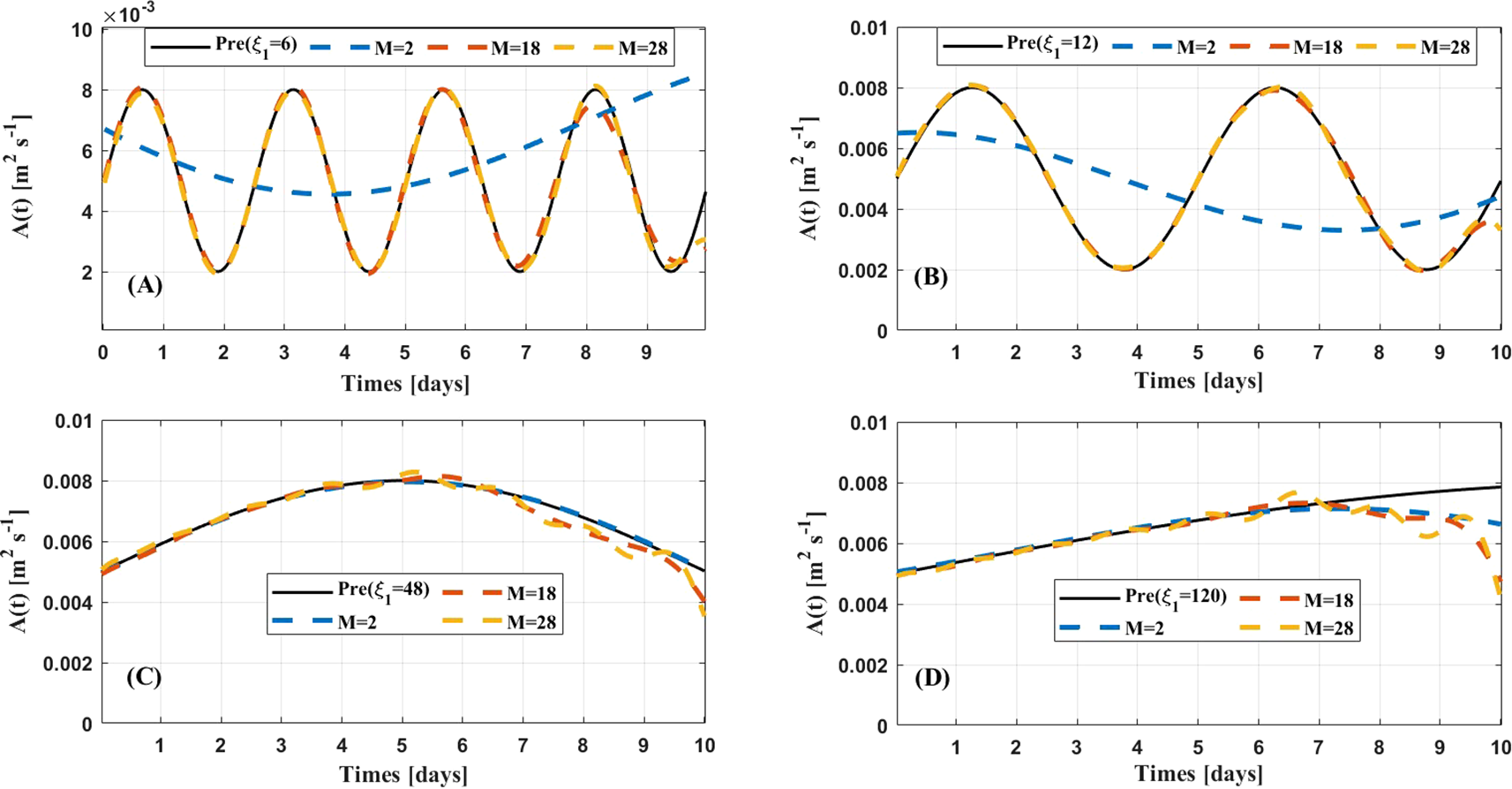
Prescribed and inverted time-dependent EVC for ξ1 = 6 (A), ξ1 = 12 (B), ξ1 = 48 (C), and ξ1 = 120 (D) in case 1.
where M is the number of terms in the summation and is determined through the trial-and-error procedures. The process for determining the values of M, γn and the maximum number of iterations for is detailed as follows. The initial guess for the EVC parameters was 0.0001 m s-1 (i.e., m s-1). The initial step length γn was set to , in accordance with previous studies (Hülsmann et al., 2010; Zhang et al., 2019). To keep the computation time within 10 minutes, the maximum number of iterations was capped at 4000, and M was set to 50. After completing the simulation process, it was observed that the cost function did not decrease with iterative steps, and the magnitude and period of the simulated EVC were significantly lower than the prescribed values. Consequently, the γn was respectively adjusted to , , and in subsequent simulation attempts. It was found that the magnitude of the simulated EVC with aligned well with the prescribed. Therefore, the step length γn was adopted as ultimately. Afterwards, the M was respectively adjusted to conduct additional simulations. It was found that the period of the simulated EVC with M = 28 matched well with the prescribed. Finally, M denoting the number of terms in Equation 36 was set to 28. The procedures for identifying the values of M, γn and iteration numbers for were consistent with the steps described above. The computation time to complete an assimilation process is approximately 6 minutes. The results at the latest iteration are used for analysis. The values of M are determined as 2, 18, and 28 eventually and the inversed are shown in Figure 1. The relationship between the cost functions and iteration steps k is illustrated in Figure 2. Values of the cost functions under various conditions after iterations are shown in Table 1.
Figure 2
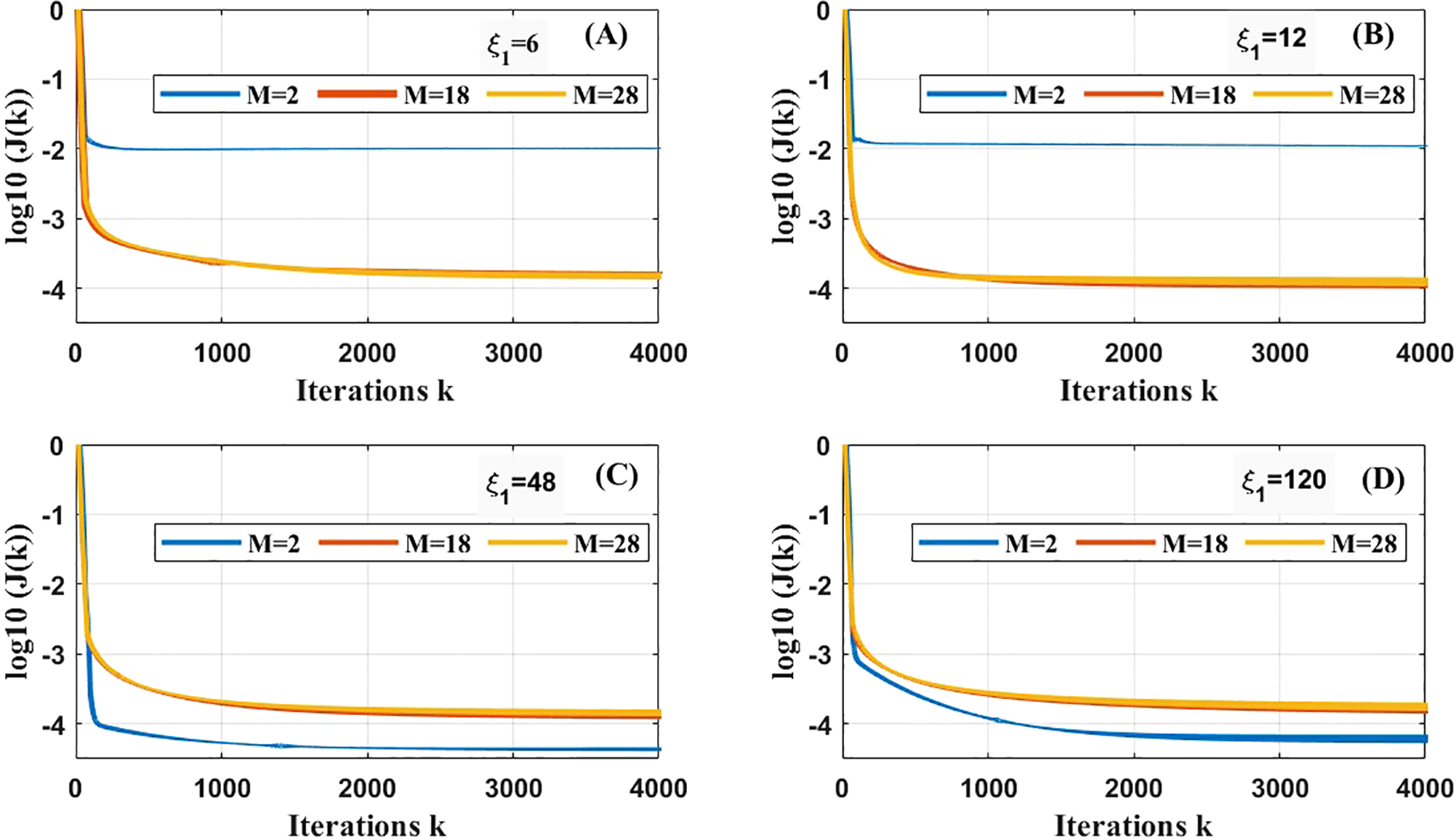
Cost functions versus iterations for ξ1 = 6 (A), ξ1 = 12 (B), ξ1 = 48 (C), and ξ1 = 120 (D) in case 1.
Table 1
| Case index | ξ 1 | M | J(k) | Case index | ξ 2 | N 1 | J(k) |
|---|---|---|---|---|---|---|---|
| 1 | 6 | 2 | 1.03×10⁻² | 2 | 0.5 | 2 | 0.51×10⁻² |
| 18 | 1.72×10⁻⁴ | 5 | 0.29×10⁻² | ||||
| 28 | 1.34×10⁻⁴ | 8 | 4.09×10⁻⁴ | ||||
| 12 | 2 | 1.09×10⁻² | 1 | 2 | 0.16×10⁻² | ||
| 18 | 1.28×10⁻⁴ | 5 | 5.74×10⁻⁵ | ||||
| 28 | 1.44×10⁻⁴ | 8 | 1.83×10⁻⁴ | ||||
| 48 | 2 | 4.06×10⁻⁵ | 2 | 2 | 5.28×10⁻⁵ | ||
| 18 | 1.16×10⁻⁴ | 5 | 3.46×10⁻⁵ | ||||
| 28 | 1.61×10⁻⁴ | 8 | 1.29×10⁻⁴ | ||||
| 120 | 2 | 7.01×10⁻⁵ | 4 | 2 | 2.73×10⁻⁵ | ||
| 18 | 1.40×10⁻⁴ | 5 | 7.29×10⁻⁵ | ||||
| 28 | 1.53×10⁻⁴ | 8 | 1.74×10⁻⁴ |
Values of cost functions after k = 4000 iterative steps in cases 1 and 2.
For the prescribed EVC with higher frequencies (i.e., and 12), the simulated EVC values with M = 18 and 28 are essentially consistent and closest to the prescribed ones (Figures 1A, B). Correspondingly, the cost functions with M = 18 and 28 decrease much faster with each iteration, reaching approximately 10–4 when the process is terminated (Figures 2A, B). The cost functions with M = 2 converge more quickly than others but only reach about 10–2 after 500 iteration steps (see Figures 2A, B). For the prescribed EVC with lower frequencies (i.e., and 120), inversional values of the EVC with M = 2 better align better with the prescribed compared to other ones (Figures 1C, D). The simulated EVC curves with M = 2 also exhibit smoother behavior than the others, particularly after 7 days, when fluctuations begin to appear in the EVC curves with M = 18 and 28 (Figures 1C, D). The values of the cost function with M = 2 continuously decrease with each iteration, approaching 10-4.5 ultimately (Figures 2C, D). The values of the cost functions with M = 18 and 28 are overlapped with the maximum remaining above 10–4 during the iterations (Figures 2C, D). This indicates that the inverted EVC with M = 2 performs better.
The experimental results indicate that the number of terms on the right-hand side of Equation 36 is related to the frequency of fluctuations in the EVC over time, i.e., . Specifically, as the frequency of variations in the EVC increases, more terms should be added to Equation 36 to enhance the accuracy of the inverted EVC. The results also suggest a reasonable range of M in Equation 36, which can help reduce computational time.
3.3 Case 2: depth-dependent EVC
In this case, the prescribed EVC is set only dependent on water depth and expressed as follows:
where ξ2 determines the EVC frequency over water depth. Four specific values of ξ2 are selected (, and the corresponding curves of the prescribed are illustrated in Figure 3. The EVC in Equation 24 is then expressed as follows:
Figure 3
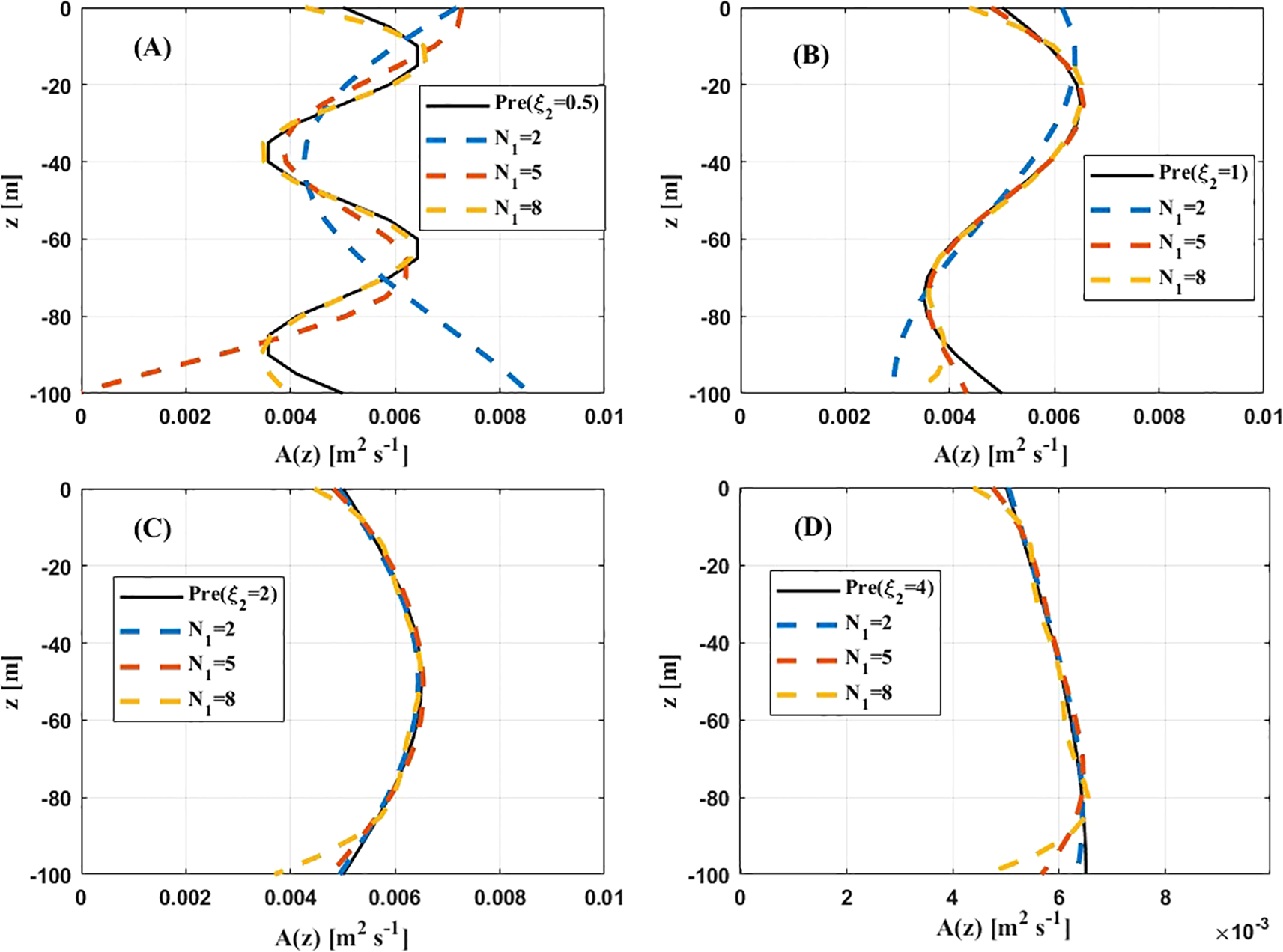
Prescribed and inverted depth-dependent EVC for ξ2 = 0.5 (A), ξ2 = 1 (B), ξ2 = 2 (C), and ξ2 = 4 (D) in case 2.
where N1 is the number of terms in the summation and determined by the trial-and-error procedure. The process of determining and the maximum iteration number is similar to that described in case 1. For , the initial guess of the EVC parameters was set to 0.0001 m s-1 (i.e., m s-1), and the step length γn was determined to be . The maximum number of iterations was set to 4000 to limit the computation time within 10 minutes. The experimental results showed that when N1 was greater than 10, there were significant errors between the simulated EVC values and the prescribed. This discrepancy caused the cost function to fail to converge during the iteration process. Ultimately, an N1 value of 8 was adopted to achieve the optimal results. The procedure for determining N1 for followed the same steps outlined above. The results from the final iteration are used for analysis. The total computation time for completing one assimilation is approximately 6 minutes. The values of N1 are selected as 2, 5, and 8 finally and the inversed are shown in Figure 3. The cost functions versus iteration steps k are illustrated in Figure 4. The values of cost functions after the data assimilation are shown in Table 1.
Figure 4
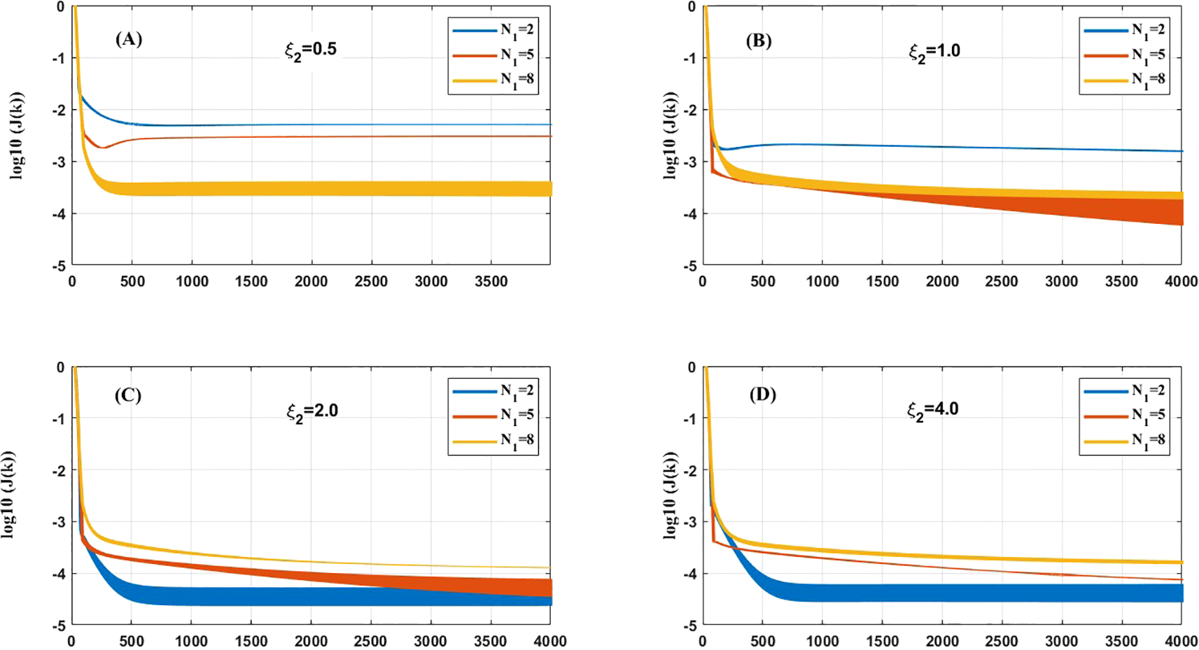
Cost functions versus iterations for ξ2 = 0.5 (A), ξ2 = 1 (B), ξ2 = 2 (C), and ξ2 = 4 (D) in case 2.
When the prescribed depth-dependent EVC adopts ξ2 = 0.5, the curve of inverted EVC with N1 = 8 is closer to the prescribed compared to the others (Figure 3A). The corresponding curve of the cost function with N1 = 8 decreases more rapidly with each iteration step and fluctuates around 10-3.5 after 2000 steps (Figure 4A). The cost functions with N1 = 2 and 5 also converge quickly, but they stabilize around 10-2.5 after 4000 steps (Figure 4A). For the prescribed EVC adopting ξ2 = 1, the simulated curves of EVC with N1 = 5 and 8 align closely with the prescribed (see Figure 4B). Notably, the curve with N1 = 5 performs the best among the three. This is also further confirmed in Figure 4B, where the average value of the cost function with N1 = 5 arrives approximately 10-3.8 when the inversion process is completed. When the prescribed EVC varies with height at low frequencies (i.e., ξ2 = 2 and 4), the curves of the inverted EVC with N1 = 2 effectively outperform others in terms of inversion (Figures 3C, D). The cost function with N1 = 2 rapidly decreases with each iterative step, eventually stabilizing around 10-4.5 after 1000 steps (Figures 4C, D). The final values of the cost functions with N1 = 2 and 5 are similar; however, the former exhibits poorer on convergence efficiency (Figures 4C, D).
The inverted results in this case indicate that the number of terms on the right-hand side of Equation 38 is relevant to the frequency of fluctuations of the EVC with depth, i.e., . Specifically, a higher frequency of variation in the EVC with water depth necessitates the inclusion of more terms in Equation 38 to improve the accuracy of the inverted EVC. The results also provide a reasonable range of M for Equation 38, which helps to reduce computational time.
3.4 Case 3: time- and depth-dependent EVC
In this case, the prescribed EVC is set dependent on time and depth, and expressed as follows:
which varies periodically, and ξ1 and ξ2 determines the EVC frequency over time and depth. Four special values of were selected: , , , and . The corresponding distributions of the prescribed are illustrated in the first columns of Figure 5. The initial guess of the parameters of EVC is set at 0.0001 m s-1 (i.e., m s-1). In contrast to cases 1 and 2, the number of iterations is set to 15000 because of the increased dimension of the EVC. The reasonable values of M, and can enhance inversion accuracy and improve the rate of convergence. Since the prescribed EVC in Equation 39 was designed according to Equations 35 and 37, the step length is set to ,which is consistent with the values used in cases 1 and 2. Correspondingly, the values of M, and in Equation 24, which represent the number of terms in the summation, should be determined based on the values used in cases 1 and 2. The optimal selections for M, and under different conditions are listed in Table 2. The computation time required to complete an assimilation is about 20 minutes. The results at the latest iteration are the most optimized and used for analysis. The related coefficients (R), root mean square errors (RMSE), and the averaged difference (AD) between the prescribed and inverted EVC, along with the cost function values, are also presented in Table 2. The inverted EVC and the scatter plot between the prescribed and inversions are shown in the second and third columns of Figure 5.
Figure 5
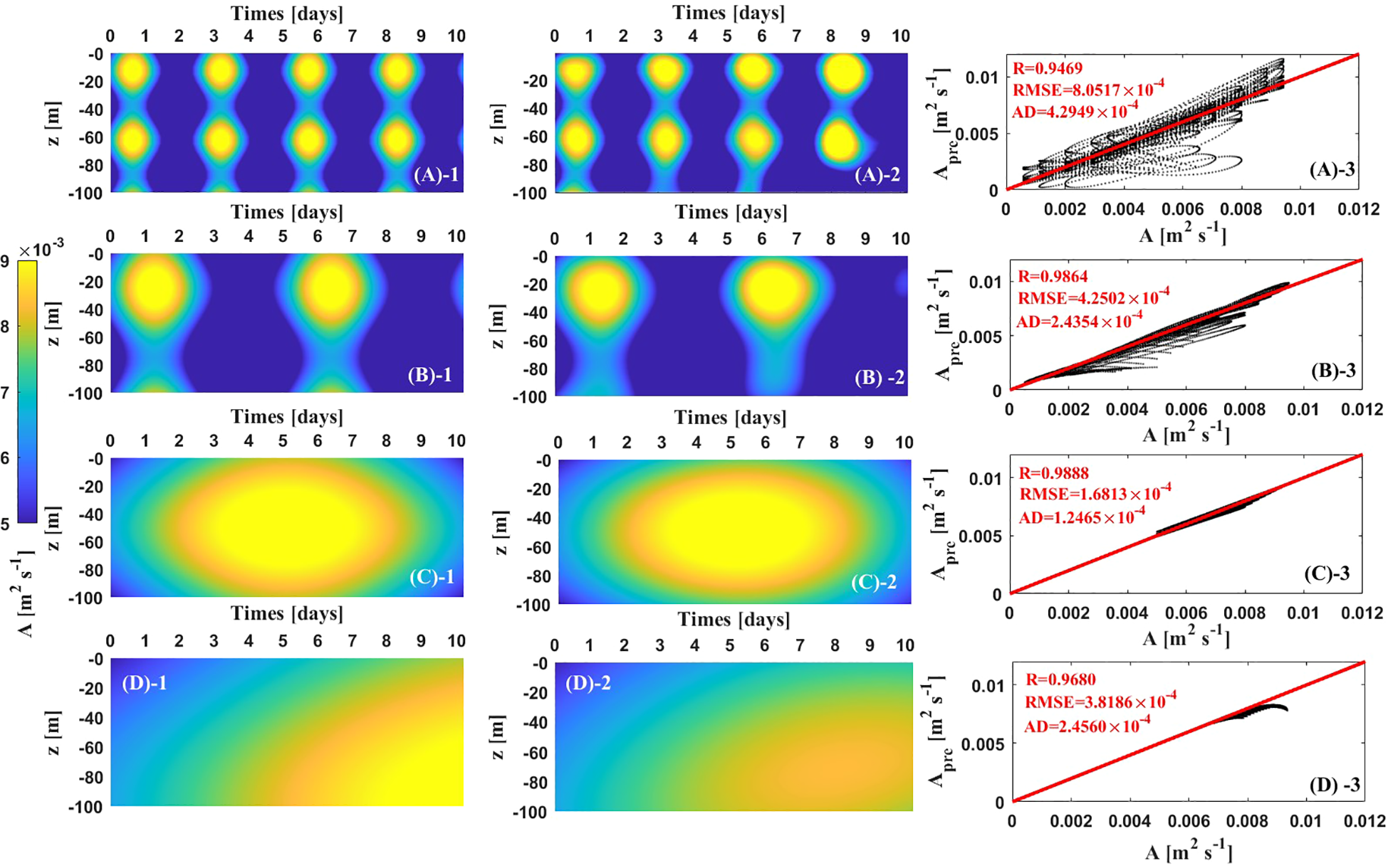
Subplots in the first column denote the prescribed A(iΔt, jΔz ) for the four values of : (A-1), (B-1), (C-1), and (D-1). Subplots in the second column denote the inverted A(iΔt, jΔz ) for the four values of : (A-2), (B-2), (C-2), and (D-2). Subplots in the third column are the scatter plot comparing the prescribed and inverted EVC.
Table 2
| Situation index | M | N 1 | N 2 | J(k) | R | RMSE | AD |
|---|---|---|---|---|---|---|---|
| 1 | 28 | 8 | 7 | 4.58×10⁻⁴ | 0.9469 | 8.05×10⁻⁴ | 4.29×10⁻⁴ |
| 2 | 18 | 5 | 4 | 5.49×10⁻⁴ | 0.9864 | 4.25×10⁻⁴ | 2.43×10⁻⁴ |
| 3 | 2 | 1 | 2 | 4.79×10⁻⁵ | 0.9888 | 1.68×10⁻⁴ | 1.24×10⁻⁴ |
| 4 | 1 | 1 | 2 | 4.81×10⁻⁵ | 0.9680 | 3.81×10⁻⁴ | 2.45×10⁻⁴ |
Values of M, N1, N2, J(k), R, RMSE and AD for different groups at k = 15000.
For the prescribed EVC with the highest frequency (i.e., ), the simulated values of the EVC at a depth of m agree well with the prescribed during the first eight days (Figures 5A-1, A-2). However, the inverted EVC values below 90 m are lower than the prescribed in certain areas, and this discrepancy becomes more apparent as the simulation time progresses. During the period from the 5th to the 10th day, the periodical variation of the EVC with time could not be accurately inverted below 90 m (Figures 5A-1, A-2). Furthermore, from the 8th to the 10th day, the simulated EVC values are significantly higher than the prescribed at a water depth of m (Figures 5A-1, A-2). The value of the cost function reaches 4.58×10⁻⁴ after sufficient iterative steps, which quantitatively reflects the inversion effect (Table 2). The scatter plot comparing the inverted and prescribed EVC indicates that the majority of the inverted EVC is close to the prescribed within the simulation domain (Figure 5A-3). The calculated R, RMSE, and AD metrics further demonstrate the model’s applicability for inverting the time- and depth- dependent EVC in this context (Table 2).
When the prescribed EVC with ) is adopted, the inverted values of the EVC at a depth at m generally accord with the prescribed values from the 1st to the 9th days (Figures 5B-1, B-2). Similar to the findings in situation 1, the simulated values of the EVC below 90 m are lower than the prescribed values in certain areas (Figures 5B-1, B-2). The inverted EVC values are slightly greater than the prescribed from the 6th to the 7th day at a depth of m. However, the periodic variation of the EVC with water depth could not be accurately simulated below 90 m (Figures 5B-1, 5B-2). The cost function value reaches 5.49×10⁻⁴ after the assimilation process stops (Table 2). The calculated values of R, RMSE, and AD are 0.9864, 4.25×10⁻⁴, 2.43×10⁻⁴ respectively, which performs better compared to those in situation 1.
For the prescribed EVC with a lower frequency (i.e., ), the effect of the inversions of EVC is prominently improved. The cost function value decreases to 4.79×10⁻⁵, which is a reduction of 0.1 compared to those in situations 1 and 3. The values of R, RMSE and AD are reduced to 0.9888, 1.68×10⁻⁴, and 1.24×10⁻⁴, respectively (Table 2). Qualitatively speaking, the inverted ECV at a depth m presents essential consistency with the prescribed value throughout the entire simulation period (Figures 5C-1, C-2). Almost all black dots are distributed on the angle bisector of the coordinate system (Figure C-3). In the last situation that the prescribed EVC varies with time and depth at the lowest frequency (i.e., ), the inverted EVC values closely match the prescribed in the anterior 7 days in the entire Ekman layer (Figures 5D-1, D-2). However, starting from the 8th day, the inverted EVC values are slightly underestimated compared to the prescribed (Figure 5D-1, D-2). The scatter plot in Figures 5D-3 along with the relevant statistical metrics indicates that the EVC in this situation is well inverted.
The inverted results indicate that the number of terms on the right side of Equation 24 is relevant to the fluctuation frequency of the EVC overt time and depth, i.e., . A higher frequency of the EVC, which varies with time and water depth, requires more terms to be added to Equation 24 for enhancing the accuracy of the inverted EVC. The model performs better when inverting the EVC that evolves over time and depth at low frequency. The results also suggest a reasonable range of in Equation 24 to optimize computational time.
3.5 Case 4: Inversion of the K-Profile Parameterization scheme affected by constant wind speeds
The distribution of the EVC remains unclear. Zhang et al. (2015) used six depth-dependent prescribed EVCs to conduct sensitivity experiments. Zhang et al. (2019) designed their prescribed time-dependent EVC to examine the reasonability and feasibility of their model. However, they did not extensively discuss how the EVC varies from low to extreme wind conditions. To address this, the K-Profile Parameterization (KPP) scheme is used as a prescribed EVC here. This scheme is commonly employed in various numerical ocean models. The dimensional form of KPP is described as follows (McWilliams et al., 2012; Song and Xu, 2013):
where , , , , , and . Unlike cases 1-3, Cd is designed to vary with the mean 10-wind speeds here, i.e., . The Cd parameterized by Kudryavtsev (2006) ranging from low to high winds is computed, and its relationship with U10 is shown in Figure 6A. The relationship between and U10 is shown in Figure 6B. For U10 exceeding 30 m s-1, a reduction of Cd or a deceleration in increments of occurs as wind speeds increase. This is attributed to the impact of sea spray. This phenomenon agrees well with some field observations and effectively characterizes the air-sea momentum exchange under varying wind conditions.
Figure 6
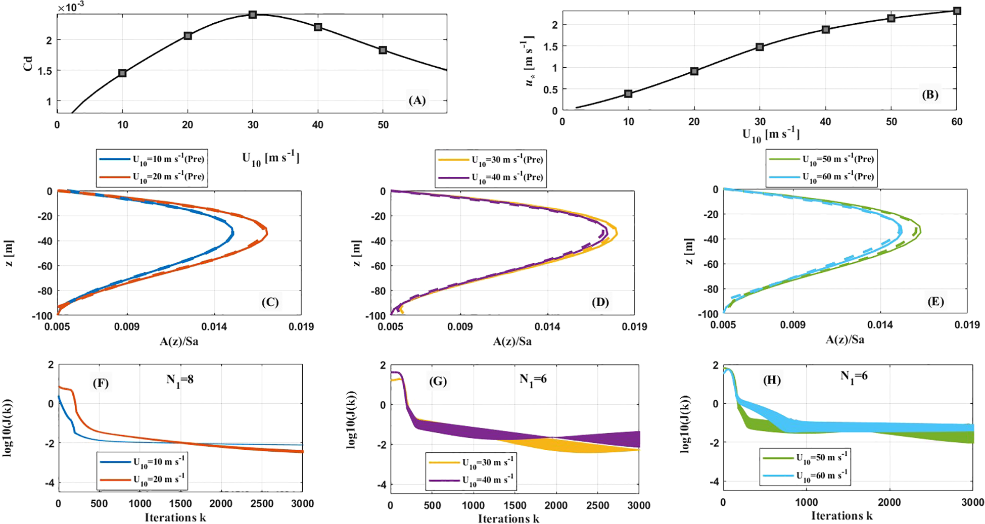
(A) versus U10. (B) versus U10. (C–E) Prescribed (solid) versus inverted EVC (dashed) at different values of U10. (F–H) Cost functions versus iterations at different U10.
Six values of U10 are selected ( m s-1), and the depth-dependent EVC in Equation 36 is adopted. The initial guess of the parameters of EVC is 0.0001 m s-1 (i.e., m s-1). The values of N1 are referenced from those in case 2 and the optimal options are presented in Table 3. Note that the step length is adjusted from to because the cost functions did not converge for greater than . Besides, since the cost functions quickly converged in this instance, the maximum number of iterations is set to 3000. The computation time to complete an assimilation is about 5 min, and the results from the final iteration are used for analysis. The inverted results along with the relationship between cost functions and iterations are illustrated in Figure 6.
Table 3
| U 10 (m s-1) | C d | N 1 | N 2 | J(k) | U 10 (m s-1) | C d | N 1 | N 2 | J(k) |
|---|---|---|---|---|---|---|---|---|---|
| 10 | 0.0014 | 8 | 8 | 40 | 0.0022 | 6 | 6 | ||
| 20 | 0.0021 | 8 | 8 | 50 | 0.0018 | 6 | 6 | ||
| 30 | 0.0024 | 6 | 6 | 60 | 0.0015 | 5 | 5 |
Values of M, N1, N2, J(k), R, RMSE and AD for different U10 at k = 3000.
In six different wind conditions, the inverted EVC in Equation 40 agrees well with the prescribed KPP profiles (Figures 6C–E). The EVC increases with water depth, reaching a maximum at a depth of 30–40 m, before decreasing and hitting a minimum at m. The corresponding values of cost functions are shown in Figures 6F–H. They converge quickly and reach around after 3000 iterative steps for U10 = 10 and 20 m s-1 (Figure 6F). The convergence of the cost functions for U10 = 30 and 40 m s-1 is less effective, as the curves exhibit larger fluctuation (Figure 6F). After sufficient iterative steps, the cost function values for U10 = 30 m s-1 fluctuate between 0.0032 and 0.0054, and those for U10 = 40 m s-1 fluctuate between 0.0067 and 0.459. The cost function values for U10 = 50 and 60 m s-1 fluctuate in ranges of 0.0087-0.0879 and 0.0363-0.0862, respectively.
The inverted results in this case suggest that the model effectively performs the inversion of the EVC as depicted by the KPP scheme. Introducing a dependent on U10 could improve the efficiency of the inversion results from low to extreme winds. After enough iteration, the cost function values present fluctuations with a larger amplitude at higher wind speeds.
3.6 Case 5: Inversion of the K-Profile Parameterization scheme affected by variable wind speeds
The variation of drag coefficients over time is considered here, i.e., . Based on the Cd defined by Kudryavtsev (2006), the relationships among Cd, U10 and time are computed and shown in Figure 7. As indicated in Section 3.1, the frequency of the variation of ua is (because of ). Consequently, the calculated Cd (or ) varies with time according to this frequency for a certain U10 (Figure 7). Note that the frequency is equal to . The prescribed dimensional EVC is set according to the KPP as follows:
Figure 7
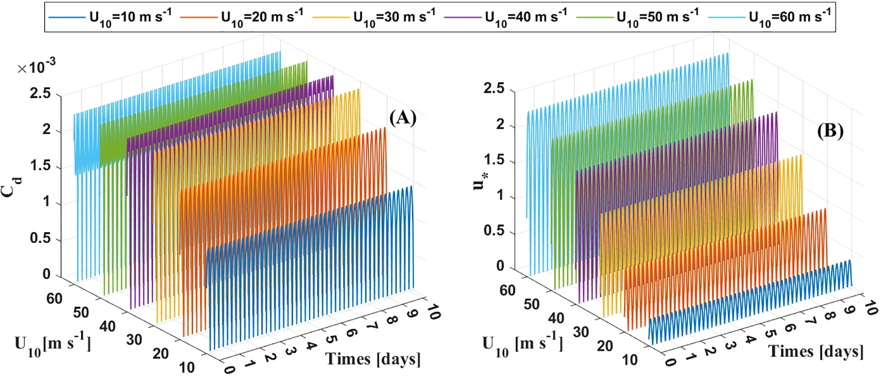
(A) versus U10 and time. (B) versus U10 and time.
where and the information on other parameters is consistent with that in Equation 36. With the increment of U10, the amplitudes of the vibration of with time increase. The distributions of the prescribed EVC for U10 = 10, 30, 50 m s-1 are illustrated in the first column of Figure 8. The prescribed also varies over time at a frequency of , similar to . It is shown that the greatest values of EVC appear within the depth range of 20 to 60 m. Within this depth range, the EVC values for U10 = 10 m s-1 are noticeably lower than those for U10 = 30 and 50 m s-1. There is little difference between the distribution of EVC for U10 = 30 and 50 m s-1. It is also displayed that the prescribed EVC periodically varies with time due to the periodic change in .
Figure 8
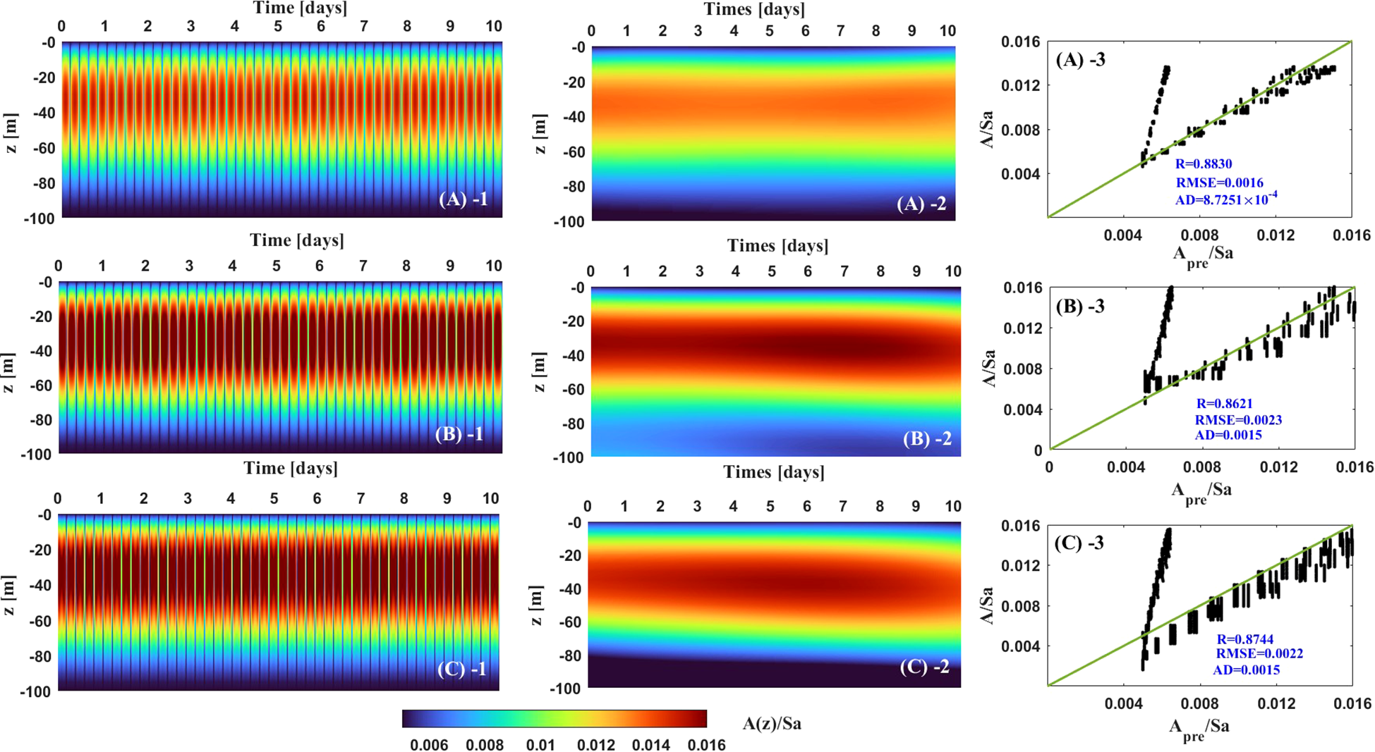
Subplots in the first column denote the prescribed A(iΔt, jΔz ) for different U10: U10 = 10 (A-1), U10 = 30 (B-1), and U10 = 50 (C-1). Subplots in the second column denote the inverted A(iΔt, jΔz ) for different U10: U10 = 10 (A-2), U10 = 30 (B-2), and U10 = 50 (C-2). Subplots in the third column are the scatter plot between the prescribed and inverted EVC for different U10: U10 = 10 (A-3), U10 = 30 (B-3), and U10 = 50 (C-3).
In the assimilation process, the initial guess of the parameters of EVC is 0.0001 m s-1 (i.e., m s-1). The iterative number was set to 10000, and the results from the final iteration are analyzed. The step length is set to according to case 4. The values of M, and are referenced from case 3, and the optimal options are listed in Table 4. The computation time to complete an assimilation was about 15 min. The temporal and spatial distributions of inverted EVC are illustrated in the second column of Figure 8. The scatter plots comparing the prescribed and inverted EVC are shown in the third column of Figure 8.
Table 4
| ua (m s-1) | M | N 1 | N 2 | J(k) | R | RMSE | AD |
|---|---|---|---|---|---|---|---|
| 2 | 8 | 7 | 0.8830 | 0.0016 | |||
| 2 | 3 | 1 | 0.8621 | 0.0023 | |||
| 2 | 2 | 1 | 0.8744 | 0.0022 |
Values of M, N1, N2, J(k), R, RMSE and AD for different groups at k = 15000.
For the three U10 conditions, the inverted EVC in Equation 41 agrees well with the prescribed ones. The maximum EVC occurs at depth of 20–60 m and that for U10 = 10 m s-1 is lower than that for U10 = 30 and 50 m s-1. The minimum EVC concentrates on the upper and bottom boundaries of the Ekman layer. However, the model is unable to invert the high-frequency variation of the EVC over time. At a certain water depth, the periodic changes in the prescribed EVC are not reflected in the inverted values. The reason for this issue is as follows. In Fourier series Equation 4, the dimensional frequency is , which is much lower than the frequency of the prescribed . As a result, the model cannot invert the high-frequency changes of the prescribed over time. The scatter plots also indicate that the inverted EVC values in certain time instants are approximately 2 to 4 times higher than the prescribed values. Most of the points are clustered around the angle bisector, and the calculated values of R are 0.8830, 0.8621, and 0.8744. This suggests that the inverted EVC coincides with the prescribed relatively well in other time instants.
The inverted results in this case indicate that the model effectively captures the inversion of the spatial and temporal distributions of the EVC prescribed by the KPP scheme. Introducing dependent on and time could improve the efficiency of the inversion results from low to extreme winds. However, the model struggles to simulate the high-frequency variations of the EVC over time.
4 Evolution of EVC during a super typhoon
4.1 Synopsis of super typhoon Hinnamnor, datasets, and methods
In this section, the model proposed in Section 2 was evaluated in real scenario to study the time- and depth-dependent EVC during a super typhoon. The super typhoon Hinnamnor, which occurred in the Northwest Pacific in 2022, was selected. The 6-hour best track of the typhoon center was downloaded from the China Meteorological Administration Tropical Cyclone Center, available at http://tcdata.typhoon.org.cn. A detailed description of the typhoon’s evolution is provided in Zhang (2023). In brief, Hinnamnor originated from a tropical depression on 28 August 2022. It intensified into a super typhoon on 30 August and maintained the replacement of its eye wall from 30 August and 1st September. The best track of the typhoon and the intensity of its center are illustrated in Figure 9A. At 0000 UTC on 31st August, the wind speed near the typhoon center exceeded 60 m s-1. At this moment, the 10-m wind field near the typhoon center is shown in Figure 9B, based on the dataset of ERA5 hourly data on single levels from 1940 to present. This dataset is a part of the ERA5 series, which are derived from the fifth generation ECMWF (i.e., European center or medium-range weather forecasts) reanalysis data, covering the past 4–7 decades. The temporal resolution of the 10-m wind speed data is one hour, and the spatial resolution is . It is available at the following website: https://cds.climate.copernicus.eu/datasets. For this analysis, meridional and zonal components of wind speeds in the range of and from 0000 UTC on 28 August to 0000 UTC on 27 September were adopted.
Figure 9
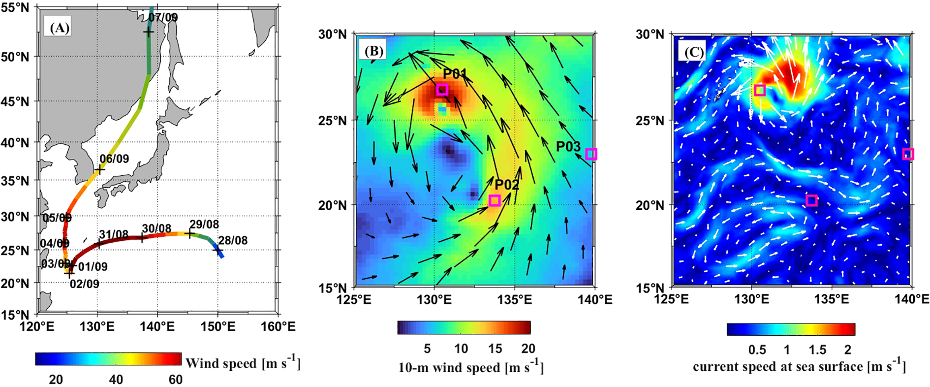
(A) Best track and intensity of typhoon Hinnamnor. Times at 0000 UTC from 30 August to 7 September are labelled. (B) The wind field near the cyclone center at 0000 UTC 31st August. (C) The surface current field near the cyclone center at 0000 UTC 31st August.
To investigate the evolution of the EVC at different wind speeds, three positions are selected, i.e., P1 , P2 , and P3 . These three locations are marked by pink squares in Figure 9B. From 28 August to 7 September 2022, the time series of the meridional and zonal components of 10-m wind speeds at these positions were obtained by applying the cubic spline interpolation method to the 10-m wind speeds from the EAR5 datasets. The results are presented in the first row of Figure 10. The duration of high wind speeds at P1 is significantly longer than that at P2 and P3 after 31st August. The maximum and at P3 is around 10 m s-1.
Figure 10
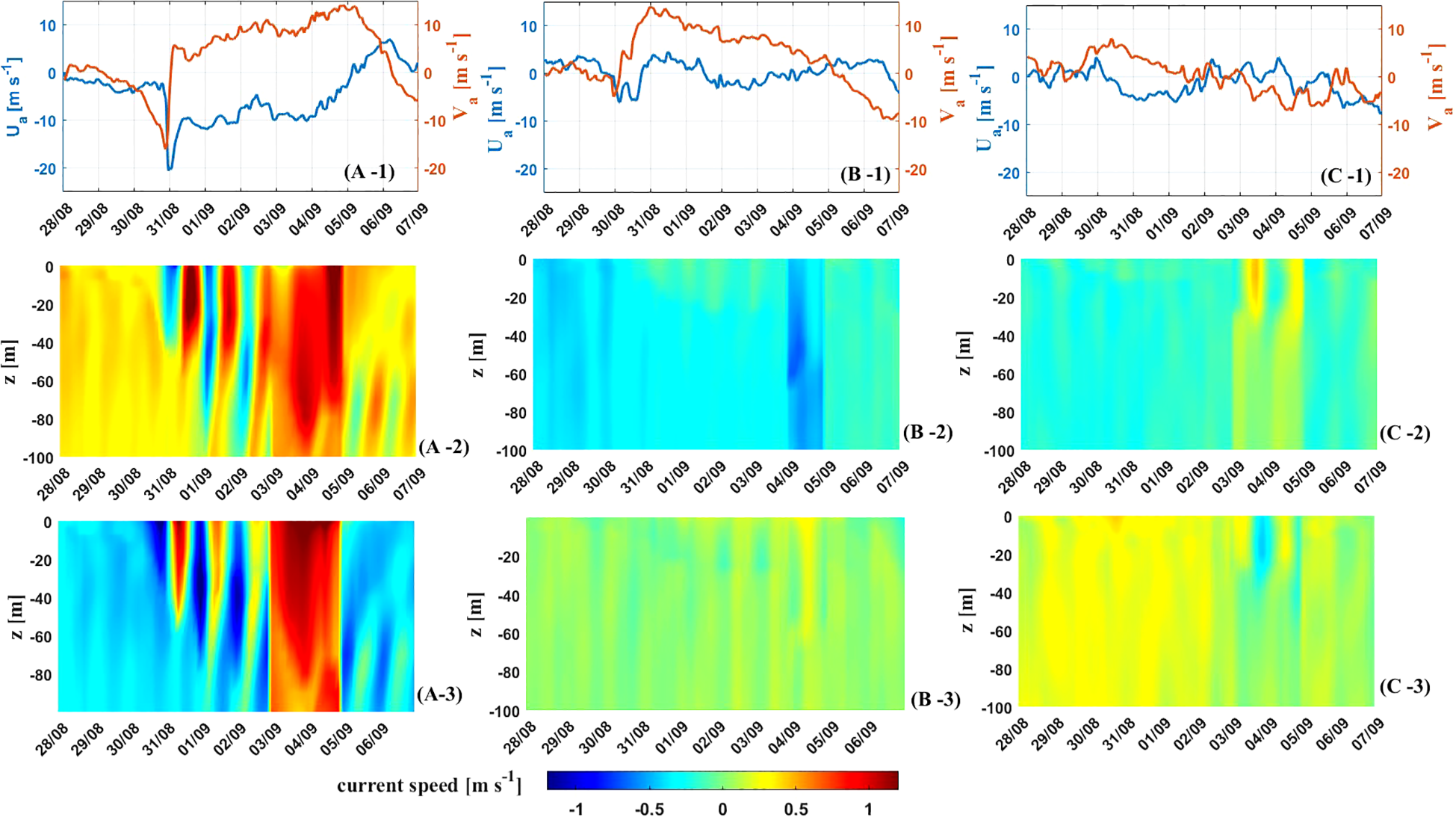
Subplots in the first row denote the time series of and at the three positions, P1 (A-1), P2 (B-1), and P3 (C-1). Subplots in the second row denote the meridional currents (i.e., ) at different positions, P1 (A-2), P2 (B-2), and P3 (C-2). Subplots in the third row denote the zonal currents (i.e., ) at different positions, P1 (A-3), P2 (B-3), and P3 (C-3).
Based on the HYCOM reanalysis data from the Global Ocean Forecasting System 3.1 (GOFS3.1), the ocean surface current at 0000 UTC on 31st August is depicted in Figure 9C. The temporal resolution of the GOFS3.1 dataset is 3 hours, horizontal resolution is and the vertical resolution is 2 m. It is available at the following website: GOFS 3.1: 41-layer HYCOM + NCODA Global 1/12° Analysis. For water depth of 0–100 m, meridional and zonal components of ocean currents in the range of and from 0000 UTC on 28 August to 0000 UTC on 27 September were adopted.Figure 9C shows that the maximum ocean surface current is located near the typhoon center.
Using the HYCOM data, the temporal and spatial distributions of ocean current velocities within water depth of 0–100 m were obtained at positions P1, P2, and P3 during the typhoon. This was done using the 2D cubic spline interpolation method, and the results are shown in the second and third rows of Figure 10. There are significant aperiodic changes in ocean current velocities over time and water depth at P1. In contrast, at P2 and P3, the current velocities show little changes with water depth and exhibit approximately periodic variations over time. According to Zhang et al. (2019), the observed currents consist of near-inertial and periodic tidal currents. The near-inertial currents include Ekman and geostrophic currents, i.e., . Therefore, is extracted by the band-pass filtered with band (Guan et al., 2014; Cao et al., 2018). The current variations due to are extracted from by removing the vertical mean values of the .
4.2 Inverted EVC and ocean current velocities at different water depths
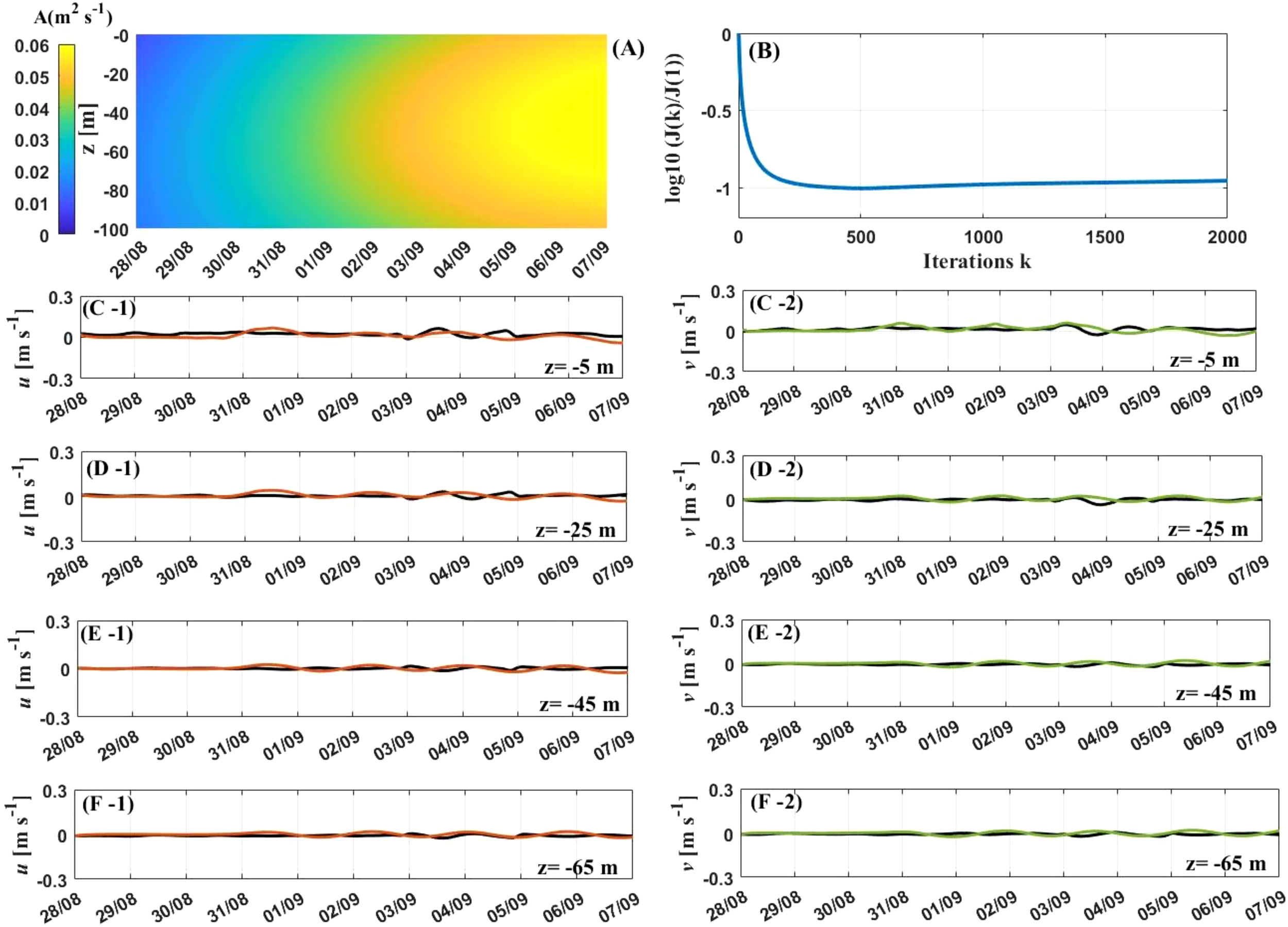
The initial guess for the parameters of EVC is 0.0001 m s-1 (i.e., m s-1). The computation time to complete an assimilation is about 10 min. The results obtained from the latest iteration are the most optimized and are used for analysis. The step length is set . The values of M, and in Equation 24 are determined by a series of trials. The best adoption of M, and is 1, 8, and 8 respectively. The final values of the inverted EVC and cost functions at P1, P2 and P3 are illustrated in the first rows of Figures 11, 12, 13. Time series for two components of the current velocities at depths of 5 m, 25 m, 45 m and 65 m are shown in the subsequent rows of Figures 11-13.
Figure 11
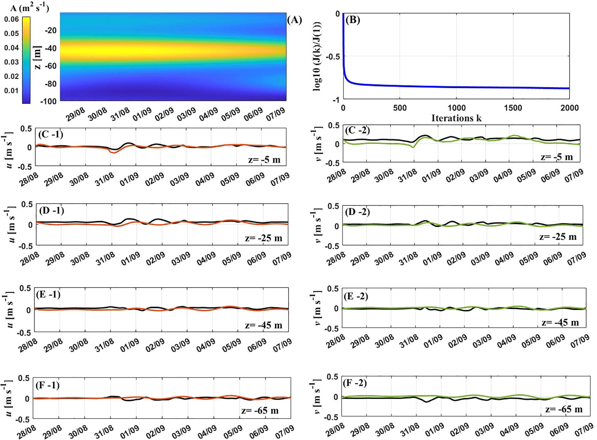
Results at P1. (A) Inverted A(iΔt, jΔz). (B) Cost functions versus iterations k. (C -1, D -1, E -1, F-1) observed (black) and inverted (red) at different depths. (C -2, D -2, E -2, F-2) observed (black) and inverted (green) at different depths.
Figure 12
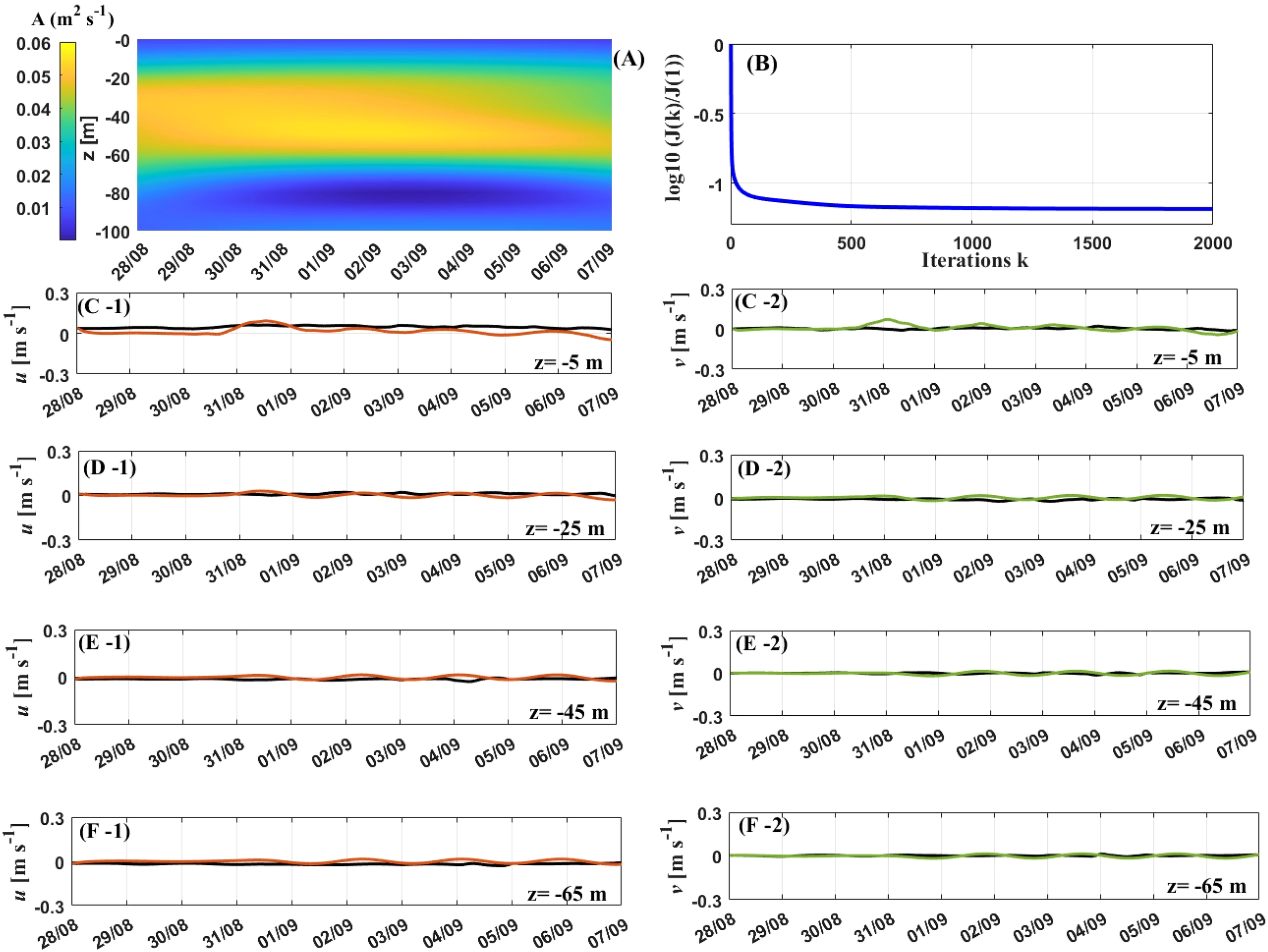
Results at P2. The rest is as the same as the caption of Figure 11.
Figure 13
Results at P3. The rest is as the same as the caption of Figure 11.
Between 28 August and 7 September, at P1, the EVC exceeded 0.05 m2 s-1 at a depth ranging from 50 to 65 m (Figure 11A). Initially, the inverted EVC increased in depth, but then it started to decrease. Wind speeds began to rise rapidly before 4 September, peaking at 20 m s-1 on 31st August (Figure 10A-1). During this period, the inverted EVC values around a depth of 50 m were at their highest. In contrast, the inverted EVC values at depths greater than 90 m remained consistently low and showed little variation over time. This indicates that the significant influence of wind speeds on EVC extends only to depths above 90 m. The cost function curve steadily decreased throughout iterative steps (Figure 11B). The slope of the curves was steep initially but approached zero after 1000 steps. The cost function decreases from 0 to -0.9 during the inversion process, indicating that the inverted EVC gradually approached the actual values. Figure 11 shows the variations in observed and simulated current velocities. From 31 August to 3 September, the observed current velocities at and m exhibit notable fluctuations. This suggests that kinetic energy is effectively transferred downwards to the upper layer of the Ekman layer in response to strong winds. This conclusion coincides with the findings of Luo et al. (2023) who conducted the simulation based on field observations. In contrast, there are no apparent fluctuations at and m. This implies that kinetic energy was unable to be transferred to the water below 45 m, even when the surface wind was strong. Figure 11 also shows that the trends of observed and simulated current velocities were identical during Hinnamnor. This revels that effect of wind speeds on the observed current velocities was consistent with their effect on simulated current velocities. Herewith, the simulated time- and depth- dependent EVC and ocean currents in the Ekman layer are reasonable.
At P2, the depth where the inverted EVC exceeded 0.05 m2 s-1 ranged from 20 to 58 m between 28 August and 7 September (Figure 12B), which is thicker than that at P1. In the water depth range of m, the inverted EVC values apparently decreased over time after 4 September. During the period of 30 August to 2 September, the wind speed consistently remained greater, but decreased from 2 to 4 September (Figure 10B-1). The wind speed sustained lower than 5 m s-1 on 2–4 September, with its direction continually shifting between north and south. This suggests that the variations in the wind direction during medium winds could enhance inverted EVC within the 20–30 m depth of the Ekman layer. The cost function curve consistently decreases with each iterative step (Figure 12B). The slop of the curve is initially steep but approach zero after 500 steps. During the inversion process, the cost function decreases from 0 to -1.2, which indicates that the inverted EVC gradually aligns with the actual. The variations in observed and simulated current velocities are illustrated in Figure 12. The similarities in the trends of the observed and simulated current velocities suggests that the inverted time- and depth-dependent EVC, along with the ocean current velocities, are meaningful.
At P3, simulated EVC values greater than 0.05 m2 s-1 occurred at depths of 0–100 m during September 3-7. The inverted EVC values increased over time at all depths, especially after 2 September. Wind speeds and changed their directions on 2 September, peaking at 8 m s-1 and 6 m s-1 respectively afterwards (Figure 10B-1). This suggests that variations in the direction of the two components of wind speed under low wind conditions could enhance the inverted EVC within the Ekman layer. The cost function consistently decreases with iterations and remains close to -1 after 1400 steps. The observed current velocities at and m apparently fluctuate on 3–5 September (Figure 13). This indicates that kinetic energy is transferred downwards to the water depth of at least 25m. The similar trends in the observed and inverted current velocities reveal that the simulated results are reliable.
5 Conclusion and discussion
The adjoint assimilation method is recognized as an effective approach for estimating the EVC. In this paper, the simulation of the time- and depth-dependent EVC is studied with the adjoint assimilation method based on the Ekman layer model. The expression of EVC is expanded into a Fourier series, which consists of four summations with parameters. The effectiveness of the simulation results is significantly influenced by the number of terms included in these summations. For the numerical experiments conducted, the GD optimization scheme is employed.
To evaluate the feasibility of the model, three groups of ideal experiments are conducted at low wind speeds. For four prescribed time-dependent EVCs with different periods, the inverted EVC after 4000 iterations performs well. The inversion results indicate that, for shorter periods, additional terms should be included in the summation related to time. Similarly, for four prescribed depth-dependent EVC with different periods, values of the inverted EVC closely match the prescribed after 4000 iterations. These results suggest that more terms should be introduced to the summation related to depth if the period is shorter. For four prescribed time- and depth-dependent EVCs with different periods, the model demonstrates improved performance in inverting EVCs that evolve over time and depth with longer periods. The experiment results indicate that the number of terms in the summation related to both depth and time should be increased when the periods are shorter. Additionally, these three groups of ideal experiments suggest a reasonable range of the number of terms in the summations.
Two additional sets of ideal experiments are carried out to study the impact of wind speeds on the inversion of the EVC. Unlike the first three groups that used a constant drag coefficient, this phase uses spray-related drag coefficients that depend on both constant wind speeds and wind speeds varying over time. In the fourth group, the depth-dependent KPP scheme is applied under six wind speeds from low to high, as the prescribed EVC. After 3000 iterative steps, the values of the inverted EVC agree well with the prescribed. The simulations results suggest that it is reasonable to apply wind-speed-related drag coefficients in the assimilation process.
In the fifth group, the time- and depth-dependent KPP scheme is designed with three different wind speeds, ranging from low to high, as the prescribed EVC. The model can effectively simulate the spatial and temporal distributions of the prescribed EVC. This also demonstrates the rationale behind using drag coefficients that are related to time-dependent wind speeds. However, the model is unable to simulate the high frequency variations of the EVC over time.
Finally, the time- and depth-dependent EVC during a super typhoon are simulated using the model. The chosen event for this analysis is super typhoon Hinnamnor, which occurred in the Northwest Pacific from 8 August to 7 September 2022. The 10-m wind fields from CCMP dataset and ocean current velocities from HYCOM model results are used as the “observations”. The greatest surface current velocities are found near the typhoon center where the wind speeds are also the strongest. At 0000 UTC on 31 August, when Hinnamnor reached the super level, three positions are chosen for analysis based on wind strength. Using the cubic spline interpolation method, the temporal and spatial evolutions in both meridional and zonal current velocities during Hinnamnor are obtained. The time series of 10-m wind speeds are also obtained by this interpolation approach. The findings indicate that current velocities are subject to significant, non-periodic changes during periods of high winds. The current velocities during low surface winds demonstrate minimal changes with water depth and vary periodically over time.
At the three positions, the normalized cost functions arrive at -0.9, -1.2 and -0.9, respectively. Additionally, the relationships between the distributions of simulated EVC and wind speeds are analysed. It is found that the EVC exceeded 0.05 m2 s-1 at depths ranging from 50 to 65 m under strong winds. The variations in one wind directions during medium winds could enhance inverted EVC within the 20–30 m depth of the Ekman layer. Furthermore, changes in the direction of the two components of wind speed under low wind conditions could enhance the inverted EVC within the Ekman layer. The observed and simulated current velocities showed identical trends during Hinnamnor, indicating that values of the inverted EVC in the Ekman layer are reasonable.
The innovation of this study stems from two key aspects: estimating the time- and depth-dependent EVC using the adjoint method for varying surface wind speeds, and applying a wind speed- and time-dependent drag coefficient as the upper boundary condition of the Ekman model. However, there are still some issues that require further investigation. The typical Ekman balance equation used in this study neglects several important processes, such as advection and stratification, which could introduce errors into the Ekman model. The sensitivity of the simulated EVC to these errors should be examined in both ideal and real cases. Furthermore, the feasibility and validity of the proposed method will be evaluated in conjunction with field observations.
Statements
Data availability statement
The original contributions presented in the study are included in the article/supplementary material. Further inquiries can be directed to the corresponding author.
Author contributions
TZ: Conceptualization, Data curation, Formal Analysis, Funding acquisition, Investigation, Methodology, Project administration, Resources, Software, Supervision, Validation, Visualization, Writing – original draft, Writing – review & editing.
Funding
The author(s) declare that financial support was received for the research and/or publication of this article. The author(s) declares financial support was received for the research, authorship, and/or publication of this article. This work is supported by the Project of the Education Department of Fujian University, grand number JAT220232, and the Research Setup Funding of Fujian University of Technology, grant number GY-Z202208.
Acknowledgments
Thanks to the colleagues in my research group for the grammar check of this manuscript.
Conflict of interest
The author declares that the research was conducted in the absence of any commercial or financial relationships that could be construed as a potential conflict of interest.
Generative AI statement
The author(s) declare that no Generative AI was used in the creation of this manuscript.
Publisher’s note
All claims expressed in this article are solely those of the authors and do not necessarily represent those of their affiliated organizations, or those of the publisher, the editors and the reviewers. Any product that may be evaluated in this article, or claim that may be made by its manufacturer, is not guaranteed or endorsed by the publisher.
References
1
Anderson D. L. T. Sheinbaum J. Hainesm K. (1996). Data assimilation in ocean models. Rep. Prog. Phys.59, 1209–1266. doi: 10.1088/0034-4885/59/10/001
2
Cao A. Z. Chen H. Fan W. He H. L. Song J. B. Zhang J. C. (2017). Estimation of eddy viscosity profile in the bottom Ekman boundary layer. J. Atmospheric Oceanic Technology.34, 2163–2175. doi: 10.1175/JTECH-D-17-0064.1
3
Cao A. Guo Z. Song J. Lv X. He H. Fan W. (2018). Near-inertial waves and their underlying mechanisms based on the South China Sea Internal Wave Experiment, (2010-2011). J. Geophysical Research: Oceans.123, 5026–5040. doi: 10.1029/2018JC01375
4
Chen H. Mao C. Lv X. Q. (2013). Estimation of open boundary conditions for an internal tidal model with an adjoint method: A comparative study on optimization methods. Math. Probl. Eng.1-12, ID802136. doi: 10.1155/2013/802136
5
Guan S. Zhao W. Huthnance J. Tian J. Wang J. (2014). Observed upper ocean response to typhoon Megi, (2010) in the northern south China sea. J. Geophys. Res. Oceans119, 3134–3157. doi: 10.1002/2013JC009661
6
Hülsmann M. Köddermann T. Vrabec J. Reith D. (2010). GROW: A gradient-based optimization workflow forthe automated development of molecular models. Comput. Phys. Commun.181, 499–513. doi: 10.1016/j.cpc.2009.10.024
7
Kazantsev E. (2012). Sensitivity of a shallow-water model to parameters. Nonlinear Anal. Real World Appl.13, 1416–1428. doi: 10.1016/j.nonrwa.2011.11.006
8
Kirincich A. R. Barth J. A. (2009). Time-varying across-shelf ekman transport and vertical eddy viscosity on the inner shelf. J. Phys. Oceanogr.39, 602–620. doi: 10.1175/2008JPO3969.1
9
Kudryavtsev V. N. (2006). On the effect of sea droplets on the atmospheric boundary layer. J. Geophys. Res.111, C070120. doi: 10.1029/2005JC002970
10
Large W. G. McWilliams J. C. Doney S. C. (1994). Oceanic vertical mixing: A review and a model with a nonlocal boundary layer parameterization. Rev. Geophys.32, 363–403. doi: 10.1029/94RG01872
11
Launder B. E. Reece G. J. Rodi W. (1975). Progress in the development of a Reynolds-stress turbulence closure. J. Fluid Mech.68, 537–566. doi: 10.1017/S0022112075001814
12
Lentz S. J. (1995). Sensitivity of the inner-shelf circulation to the form of the eddy viscosity profile. J. Phys. Oceanography25, 19–28. doi: 10.1175/1520-0485(1995)025<0019:SOTISC>2.0.CO;2
13
Liu D. C. Nocedal J. (1989). On the limited memory BFGS method for large scale optimization. Math. Program.45, 503–528. doi: 10.1007/BF01589116
14
Luo C. Gao G. Xu M. Yin B. Lv X. (2023). A study of wind stress effects on the vertical eddy viscosity coefficient using the ekman model with data assimilation. J. Marine Sci. Engineering.11, 1487. doi: 10.3390/jmse11081487
15
McWilliams J. C. Huckle E. Liang J. H. Sullivan P. P. (2012). The wavy Ekman layer: Langmuir circulations, breaking waves, and Reynolds stress. J. Phys. Oceanogr.42, 1793–1816. doi: 10.1175/JPO-D-12-07.1
16
Mellor G. L. Yamada T. (1982). Development of a turbulence closure model for geophysical fluid problems. Rev. Geophys. Space Phys.20, 851–875. doi: 10.1029/RG020i004p00851
17
Nie Y. Wang Y. Lv X. (2019). Acquiring the arctic-scale spatial distribution of snow depth based on AMSR-E snow depth product. J. Atmos. Ocean. Technol.36, 1957–1965. doi: 10.1175/JTECH-D-18-0217.1
18
Obermeier F. (2006). Prandtl’s mixing length model-Revisited. Proc. Appl. Math. Mech.6, 577–578. doi: 10.1002/pamm.200610269
19
Rai S. Hecht M. Maltrud M. Aluie H. (2021). Scale of oceanic eddy killing by wind from global satellite observations. Sci. Adv.7, 1–9. doi: 10.1126/sciadv.abf4920
20
Roach C. J. Phillips H. E. Bindoff N. L. Rintoulet S. R. (2015). Detecting and characterizing Ekman currents in the Southern Ocean. J. Phys. Oceanogr.45, 1205–1223. doi: 10.1175/JPO-D-14-0115.1
21
Shanno D. F. Phua K. H. (1980). Remark on “Algorithm 500: Minimization of Unconstrained Multivariate Functions [E4]”. ACM Trans. Math. Softw.6, 618–622. doi: 10.1145/355921.355933
22
Song J. B. Xu J. L. (2013). Wave-modified Ekman current solutions for the vertical eddy viscosity formulated by K-Profile Parameterization scheme. Deep Sea Res. Part I: Oceanographic Res. Papers80, 58–65. doi: 10.1016/j.dsr.2013.05.009
23
Wirth A. (2010). On the Ekman spiral with an anisotropic eddy viscosity. Bound. Layer Meteor.137, 327–331. doi: 10.1007/s10546-010-9527-7
24
Wu X. Xu M. Gao Y. Lv X. (2021). A scheme for estimating time-varying wind stress drag coefficient in the ekman model with adjoint assimilation. J. Mar. Sci. Eng.9, 1220. doi: 10.3390/jmse9111220
25
Wu X. Xu M. Gao G. Yin B. Lv X. (2022). Application of the trigonometric polynomial interpolation for the estimation of the vertical eddy viscosity coefficient based on the ekman adjoint assimilation model. J. Mar. Sci. Eng.10, 1165. doi: 10.3390/jmse10081165
26
Yi J. C. Gao Y. Q. Zhang J. C. (2018). Estimation of the time-varying vertical eddy viscosity coefficient in an ekman layer model through the adjoint data assimilation approach. Mar. Sci.42, 71–82. doi: 10.11759/hykx20180408002
27
Yoshikawa Y. Endoh T. (2015). Estimating the eddy viscosity profile from velocity spirals in the Ekman boundary layer. J. Atmos. Oceanic Technol.32, 793–804. doi: 10.1175/JTECH-D-14-00090.1
28
Yu L. O’Brien J. J. (1991). Variational estimation of the wind stress drag coefficient and the oceanic eddy viscosity profile. J. Phys. Oceanogr.21, 709–719. doi: 10.1175/1520-0485(1991)021,0709:VEOTWS.2.0.CO;2
29
Zhang T. (2023). Features of upper ocean and surface waves during the passage of super typhoon Hinnamnor (2022). Front. Marine Sci.10. doi: 10.3389/fmars.2023.1275565
30
Zhang Q. Gao Y. Lv X. (2015). Estimation of oceanic eddy viscosity profile and wind stress drag coefficient using adjoint method. Math. Probl. Eng.1-11, ID309525. doi: 10.1155/2015/309525
31
Zhang J. Li G. Yi J. Gao Y. Cao A. (2019). A method on estimating time-varying vertical eddy viscosity for an Ekman layer model with data assimilation. J. Atmospheric Oceanic Technology.36, 1789–1812. doi: 10.1175/JTECH-D-18-0223.1
32
Zhang J. Lv X. Q. (2010). Inversion of three-dimensional tidal currents in marginal seas by assimilating satellite altimetry. Comput. Methods Appl. Mech. Eng.199, 3125–3136. doi: 10.1016/j.cma.2010.06.014
33
Zhang Y. W. Tian. J. W. Xie L. L. (2009). Estimation of eddy viscosity on the South China Sea shelf with adjoint assimilation method. Acta Oceanologica Sinica.5), 9–16.
34
Zhu Y. Navon I. M. (1999). Impact of parameter estimation on the performance of the FSU global spectral model using its fullphysics adjoint. Mon. Wea. Rev.127, 1497–1517. doi: 10.1175/1520-0493(1999)127,1497:IOPEOT.2.0.CO;2
Summary
Keywords
eddy viscosity coefficient, Ekman model, adjoint method, drag coefficient, wind speeds
Citation
Zhang T (2025) Application of adjoint method to the evaluation of temporal and spatial variations of the eddy viscosity coefficient. Front. Mar. Sci. 12:1573004. doi: 10.3389/fmars.2025.1573004
Received
08 February 2025
Accepted
25 April 2025
Published
16 May 2025
Volume
12 - 2025
Edited by
Matthieu Le Hénaff, Atlantic Oceanographic and Meteorological Laboratory (NOAA), United States
Reviewed by
Xueen Chen, Ocean University of China, China
Calin Martin, University of Vienna, Austria
Updates
Copyright
© 2025 Zhang.
This is an open-access article distributed under the terms of the Creative Commons Attribution License (CC BY). The use, distribution or reproduction in other forums is permitted, provided the original author(s) and the copyright owner(s) are credited and that the original publication in this journal is cited, in accordance with accepted academic practice. No use, distribution or reproduction is permitted which does not comply with these terms.
*Correspondence: Ting Zhang, Zhangting2021@fjut.edu.cn
Disclaimer
All claims expressed in this article are solely those of the authors and do not necessarily represent those of their affiliated organizations, or those of the publisher, the editors and the reviewers. Any product that may be evaluated in this article or claim that may be made by its manufacturer is not guaranteed or endorsed by the publisher.