 Xiaoci Wu1,2
 Wei Yu
- 1Ocean Decade International Cooperation Center (ODCC), Qingdao, China
- 2College of Marine Living Resource Sciences and Management, Shanghai Ocean University, Shanghai, China
- 3National Engineering Research Center for Oceanic Fisheries, Shanghai Ocean University, Shanghai, China
- 4Key Laboratory of Sustainable Exploitation of Oceanic Fisheries Resources, Ministry of Education, Shanghai Ocean University, Shanghai, China
- 5Key Laboratory of Oceanic Fisheries Exploration, Ministry of Agriculture and Rural Affairs, Shanghai, China
Jumbo flying squid (Dosidicus gigas), an essential commercial fisheries species in the Humboldt Current System (HCS), is highly sensitive to changes in the marine environment. Mesoscale eddies are prevalent oceanographic phenomena that play a pivotal role in circulation, material transport, and ecosystem dynamics within the ocean. The waters off Chile in the south-central part of the HCS serve as one of the primary fishing grounds for D. gigas. This region is characterized by active mesoscale eddies that regulate biogeochemical processes. However, the impacts of mesoscale eddies on D. gigas off Chile remain unclear. To address this knowledge gap, this study analyzed the spatiotemporal distribution of mesoscale eddies in this region using a global mesoscale eddy dataset. By integrating environmental and D. gigas fishing data, we assessed the influence of these mesoscale eddies, and their associated environmental changes, on the abundance and distribution of D. gigas. Results revealed that mesoscale eddies were mainly formed in the coastal areas of Chile, with monthly and annual variations in their occurrences. A positive correlation was observed between the number of eddies and the abundance of D. gigas. Cyclonic eddies (CEs) were found to harbor a higher aggregation of D. gigas compared to anticyclonic eddies (AEs). An analysis of the proportion of key environmental factors within suitable ranges for the two types of eddies indicated that the number and proportion of key environmental factors—particularly sea surface temperature (SST)—within suitable ranges were higher in CEs. This study concludes that CEs provide more suitable environmental conditions than AEs, thereby supporting the aggregation of D. gigas.
1 Introduction
Eastern boundary upwelling systems make a significant contribution to global ocean productivity (Bograd et al., 2023) by replacing warm, nutrient-poor waters with cold, nutrient-rich waters from the deep ocean. The Humboldt Current System (HCS), located near the equator, spans the western coast of South America from Peru to Chile, encompassing much of the southeastern Pacific Ocean coastline (Thiel et al., 2007). This system is characterized by a shallow, yet intense, oxygen minimum zone (Gutiérrez et al., 2016) and is significantly influenced by the El Niño-Southern Oscillation (Espinoza-Morriberón et al., 2017; Montecinos and Gomez, 2010). Driven by upwelling processes, the HCS is highly productive (Chavez and Messié, 2009; Keith et al., 2020), resulting in high fishery productivity in the region. Previous studies (Chavez et al., 2008) have revealed that the HCS accounts for over 10% of the total global fishery production, with its northern waters considered the most productive region in terms of fish yield per unit area. Jumbo flying squid (Dosidicus gigas) is one of the primary commercial targets within this system (Mariano Gutiérrez et al., 2017).
Cephalopods are recognized by the Food and Agriculture Organization of the United Nations as one of the three most promising fishery resources for economic development in the world’s oceans (Chen, 2019). Among these, D. gigas stands out as one of the largest, most abundant, and highest-yielding species. Dosidicus gigas exhibits diel vertical migration behavior (Sakai et al., 2017) and inhabits waters from 0 to 1200 meters depth (Ibáñez et al., 2016). Its population structure is relatively complex and can be classified using various methods. For example, they can be divided into three size-based populations based on mantle length: large, medium, and small (Nigmatullin, 2001). Alternatively, molecular biology techniques distinguish two distinct groups, one in the Northern Hemisphere and the other in the Southern Hemisphere (Sandoval-Castellanos et al., 2007). In the marine food web, D. gigas is an active predator with a broad dietary spectrum, providing an important link between higher trophic level consumers and lower trophic level species (Gonzalez-Pestana et al., 2022; Markaida, 2006; Nigmatullin, 2001). As a short-lived species with a typical lifespan of no more than one year, D. gigas is highly sensitive to changes in the marine environment. All life history processes of the species are influenced by environmental fluctuations (Wen et al., 2024). For instance, an analysis of the stomach contents of D. gigas in the Gulf of California before, during, and after El Niño events, revealed environmental-based dietary shifts. In warmer, less productive environments, it predominantly fed on low-calorie prey such as euphausiids and pteropods. Conversely, in relatively cooler, nutrient rich (or relatively warmer yet nutrient rich) environments, its diet comprised large quantities of small, high-energy prey such as anchovies (Portner et al., 2020).
Mesoscale eddies are a prevalent natural oceanographic phenomenon characterized by self-sustaining rotating water masses that persist for days to months, influencing spatial scales of tens to hundreds of kilometers (Chelton et al., 2007, Chelton et al., 2011). These eddies are typically classified into two types: cyclonic eddies (CEs), which induce water divergence and upwelling at their centers, and anticyclonic eddies (AEs), which exhibit the opposite effects (Bakun, 2006). Mesoscale eddies account for most of the kinetic energy in the global ocean (Wang et al., 2023) and play a crucial role in regulating oceanic heat and salinity transport, water mass distribution, carbon cycling, and sound propagation (Bakun, 2006; Dong et al., 2014; Jersild et al., 2021; Jian et al., 2009). They can also profoundly affect the abundance and distribution of marine organisms across trophic levels (Choi et al., 2013; Garcia et al., 2022; Gaube et al., 2018; Matis et al., 2014; Receveur et al., 2024; Xing et al., 2023, Xing et al., 2024). For example, in the North Atlantic Ocean, bluefin tuna spawn within AEs, thereby excluding weaker-swimming predators or competitors and enhancing their survival rates (Bakun, 2006). Moreover, mesoscale eddies can influence fishing activities, for example, tuna fishing operations are concentrated within AEs (Xing et al., 2023). Therefore, elucidating the mechanisms by which mesoscale eddies affect marine organisms across different trophic levels can provide scientific guidance for fisheries managers, enabling them to optimize fishing activities and ensure the sustainable development of fishery resources.
Chilean waters, located in the mid-southern region of the HCS, are characterized by a widespread presence of mesoscale eddies (Chaigneau et al., 2009), which play a pivotal role in regulating regional productivity (Hormazabal et al., 2004). Here, D. gigas is a significant commercial fishing target as it is widely distributed (Feng et al., 2022), however, its distribution and diel vertical migration are influenced by mesoscale eddies (Arkhipkin et al., 2015, Arkhipkin et al., 2023; Watanabe et al., 2006). Previous studies have shown that the evolution and type of mesoscale eddy in the northern region of the HCS significantly impact the abundance and distribution of D. gigas (Jin et al., 2024; Wu et al., 2024). However, species responses to mesoscale eddies may vary across different regions (Durán Gómez et al., 2020; Hsu et al., 2015). Therefore, it is essential to investigate the responses of D. gigas abundance and distribution to mesoscale eddies and its underlying mechanisms in other regions.
Thus, this study analyzed the spatiotemporal variations of mesoscale eddies and the resulting changes in D. gigas abundance and distribution, with a particular focus on the differential effects of eddy types. The findings aim to provide scientific insights for the sustainable development of oceanic cephalopod fisheries.
2 Materials and methods
2.1 Fisheries data
The D. gigas longline fishing data utilized in this study were provided by the China Distant-Water Fisheries Data Center at Shanghai Ocean University. The dataset included information on fishing locations (longitude and latitude, with a spatial resolution of 0.001°), fishing dates (year, month, and day), catch (in tons), and fishing effort (number of operational days). The temporal coverage of the data spanned March to May 2016 to 2021, with a spatial range of 70°–97°W and 20°–47°S. Additionally, catch per unit effort (CPUE), calculated as the ratio of catch to fishing effort, was used as an indicator of D. gigas abundance.
2.2 Environmental data
Sea surface height (SSH), sea surface salinity (SSS), mixed layer depth (MLD), sea surface temperature (SST), temperature at 200 m depth (TEM200), and temperature at 400 m depth (TEM400) were obtained from the global ocean physics reanalysis product provided by the Copernicus Marine Environment Monitoring Service (CMEMS) (https://data.marine.copernicus.eu/product/GLOBAL_MULTIYEAR_PHY_001_030/description), with a temporal resolution of daily and a spatial resolution of 0.083°. Chlorophyll-a concentration (Chl-a), sea surface dissolved oxygen concentration (DO), dissolved oxygen concentration at 200 m depth (DO200), and dissolved oxygen concentration at 400 m depth (DO400) were sourced from the CMEMS global ocean biogeochemical hindcast product (https://data.marine.copernicus.eu/product/GLOBAL_MULTIYEAR_BGC_001_029/description), with a temporal resolution of daily and a spatial resolution of 0.25°. All environmental data encompassed the required spatial and temporal extent of the study area. The linear interpolation method was used to match the fisheries data with the environmental data.
2.3 Mesoscale eddy data
The altimetric Mesoscale Eddy Trajectories Atlas (META3.2 DT), produced by SSALTO/DUACS and distributed by AVISO+ (https://aviso.altimetry.fr) with support from CNES in collaboration with IMEDEA, was developed using the enhanced eddy py-eddy-tracker algorithm applied to absolute dynamic topography maps (Pegliasco et al., 2022). This dataset has been successfully applied in numerous studies (Wang et al., 2023; Xing et al., 2023, Xing et al., 2024; Yun et al., 2024) and is available in two versions. For this study, the all-satellites version was utilized, covering global eddy information from 1 January 1993 to 9 February 2022. This dataset provided daily data on eddy radius, type, core location, and boundaries. We selected all eddies from this dataset within the time range of 2016–2021 and the spatial range of 70°–97°W and 20°–47°S. The filtered results were compiled into a new dataset, which includes a total of 8,463 eddies (all with a lifetime exceeding 10 days), comprising 4,511 CEs and 3,952 AEs.
2.4 Data analysis of the relationship between eddies and D. gigas abundance and distribution
The annual and monthly variations in D. gigas CPUE and the number of eddies that occurred from March to May 2016 to 2021 were statistically analyzed. The Pearson correlation coefficient was used to assess the relationship between the D. gigas CPUE and eddy numbers across different temporal scales.
The influence range of the eddy was defined as twice its actual boundary, represented by a circular grid. This circular grid had a radius of 2R (where R is the radius of a circle with the same area as the eddy’s actual boundary), with its center positioned at the eddy center (Gaube et al., 2017; Wu et al., 2024). Each fishing location was assigned to the nearest eddy based on its distance to the eddy center, and its spatial distribution within the corresponding circular grid was analyzed. Additionally, the distributions of D. gigas catch, fishing effort, and CPUE within the influence range of eddies were quantified.
A Generalized Additive Model (GAM) was used to explore the potential relationships between D. gigas abundance and mesoscale eddy structures. Prior to model construction, 0.1 was added to the abundance values to avoid the occurrence of zero values, and all explanatory variables were tested for multicollinearity using the Variance Inflation Factor (VIF) (O’brien, 2007). The GAM was constructed in R using the mgcv package (Wood, 2006). The formulation of the GAM was as follows:
where, s was the smooth spline; radius represented the radius of the CE or AE; velocity referred to the velocity of the CE or AE; amplitude was the radius of the CE or AE; lon and lat correspond to the CE or AE center’s longitude and latitude, respectively; distance was the distance between the fishing location and the CE or AE center; and ϵ denoted the random error.
2.5 Analysis of the influence of environmental factors on D. gigas abundance
This study employed a random forest (RF) analysis to assess the influence of the ten environmental factors described in Section 2.2 on the abundance of D. gigas. The RF algorithm is an ensemble learning method based on decision trees (Breiman, 2001), capable of measuring the importance of predictor variables (Zhang and Lu, 2012), and is typically effective in prediction accuracy while avoiding overfitting (Prasad et al., 2006). It has been successfully applied across various fields including oceanography, fisheries science, ecology, and agronomy (Camacho et al., 2019; Cutler et al., 2007; Everingham et al., 2016; Giamalaki et al., 2022). The percentage increase in mean squared error (%IncMSE) was used to gauge the importance of predictor variables with higher %IncMSE values indicating greater significance. In most cases, the default parameter settings of the RF yield satisfactory results (Probst et al., 2019). Prior to constructing the RF model, multicollinearity among the ten environmental factors was examined using the VIF, which indicated no significant multicollinearity (all VIF values were below 10) (Table 1) (O’brien, 2007). Therefore, all ten environmental factors served as predictor variables in the RF, with D. gigas CPUE as the response variable, mtry set to 3, ntree set to 500, and all other parameters were set to default. The RF was implemented in R version 4.4.0 using the “randomForest” package (Liaw and Wiener, 2002). Additionally, the significance of different predictor variables in the RF model was analyzed using the “rfPermut” package. Based on the importance scores and significance (p<0.05) derived from the RF analysis, key environmental factors influencing the abundance of D. gigas were selected.

Table 1. Variance inflation factor (VIF) test results.
2.6 Distribution analysis of key environmental factors influencing D. gigas within eddies
Using the frequency distribution method, the key environmental factors identified in Section 2.5 were classified into different intervals. The total catch and fishing effort within each interval were then computed, and the environmental factor intervals corresponding to the maximum catch and effort were defined as the optimal range.
Eddy grids within the influence range that contained fishing points were selected, as described in Section 2.4. We then analyzed the distribution of the selected key environmental factors within these eddy grids, averaging the results for CE and AE grids separately, to explore the variation in environmental factor distribution between the two types of eddies. Furthermore, we calculated the proportion of optimal environmental factor intervals within both types of eddy grids.
3 Results
3.1 The spatiotemporal distribution and propagation trajectories of mesoscale eddies in Chilean waters
By categorizing each eddy based on its initiation date into respective months and years, distinct monthly and annual patterns in CE and AE numbers were identified (Figures 1A–D). Both CEs and AEs exhibited an overall monthly trend of an initial increase in numbers, with a subsequent decline. The number of CEs peaked in July (420 eddies) and reached its minimum in December (294 eddies), while the number of AEs peaked in August (374 eddies) and was lowest in February (266 eddies). The number of CEs and AEs showed differing annual trends. From 2015 to 2021, the annual number of CEs consistently surpassed that of AEs. Notably, in 2020, the disparity between CE and AE numbers was the greatest, with a difference of 165 eddies.

Figure 1. (A) Monthly variations, (C) interannual trends, and (E) relative propagation trajectories of CEs within the study area; (B) Monthly variations, (D) interannual trends, and (F) relative propagation trajectories of AEs within the study area.
By defining the origin of each eddy as 0°, 0°, the propagation trajectories throughout their entire lifecycles were visualized (Figures 1E, F). The results revealed distinct longitudinal propagation characteristics, with approximately 82% of CEs and 84% of AEs moving westward. Latitudinally, around 60% of the total number of eddies propagated northward. The maximum propagation distance reached approximately 1752 km (CEs) and 1693 km (AEs), with the westward movement spanning around 16°for both eddy types, the southward movement covering roughly 4°for CEs and, the northward movement around 8°for AEs.
The initial detected position of an eddy’s center was defined as its generation location. To analyze the spatial distribution characteristics of eddy generation, the study area was divided into 0.5° × 0.5° grid cells and the number of eddies generated within each grid cell between 2015 and 2021 was calculated (Figure 2). The primary regions of eddy generation were located in the coastal waters east of 80°W along the Chilean coastline. Overall, the number of eddies increased from the northwest to the southeast.
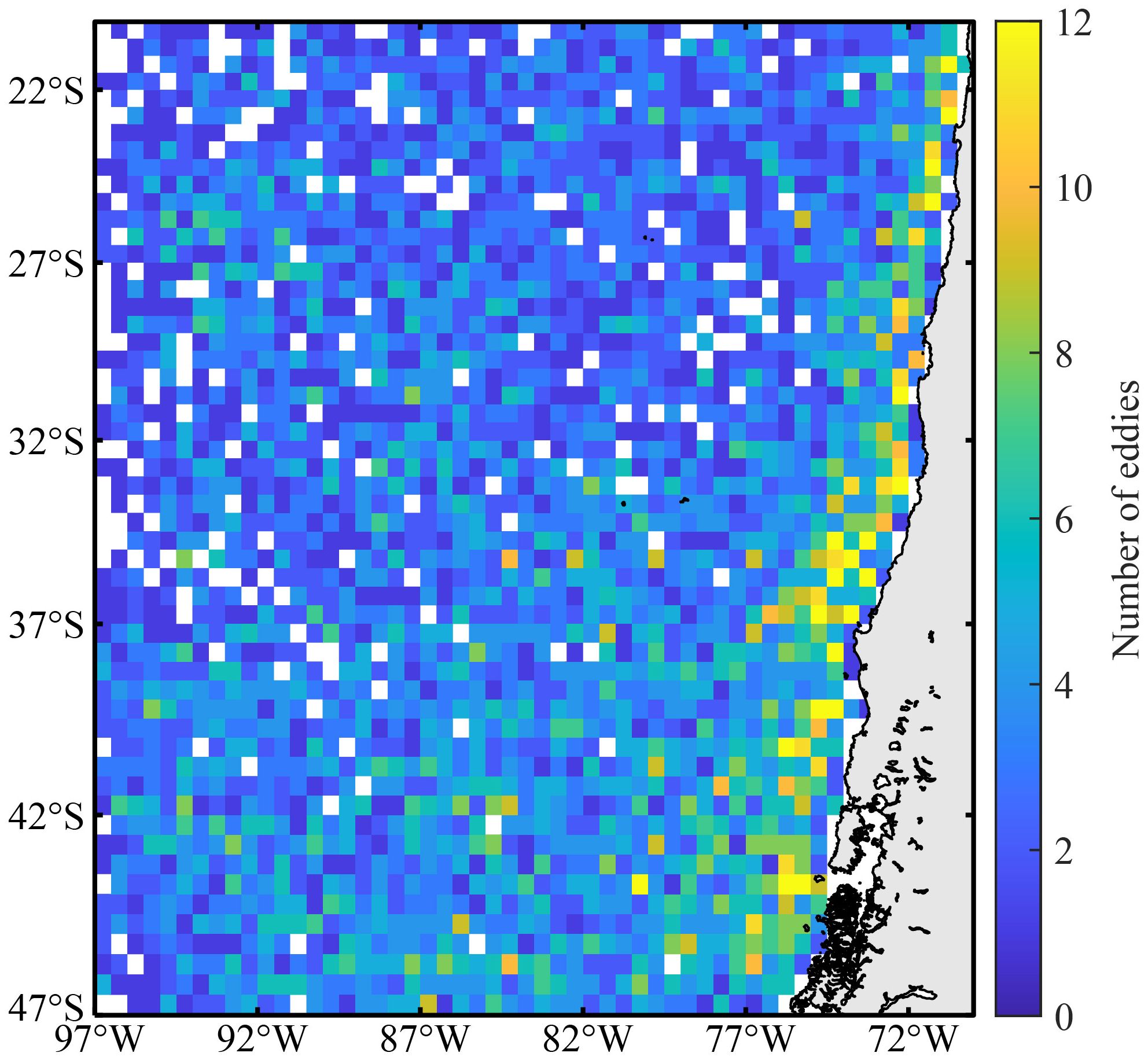
Figure 2. The spatial distribution of eddy generation locations off Chile from 2015 to 2021.
Eddy lifetime was categorized into different groups, and the number and proportion of eddies within each group were calculated (Table 2). The results indicated that 51.74% of the eddies had a lifetime of less than 30 days, 44.15% had a lifetime between 30 and 180 days, and 4.1% had a lifetime exceeding 180 days. Additionally, CEs were more prevalent when the lifetime was under 180 days, whereas AEs were more abundant when the lifetime exceeded 180 days.
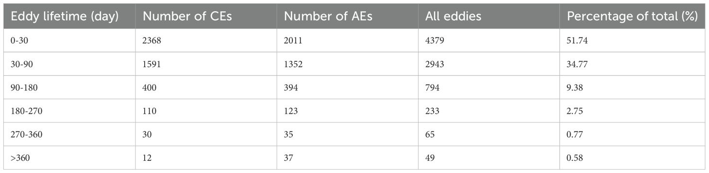
Table 2. Number and percentage of eddies across different lifetime ranges.
3.2 The relationship between eddies and D. gigas abundance off Chile
The statistical analysis revealed a monthly and annual correlation between the number of eddies and the CPUE of D. gigas (Figure 3). From March to May, eddy numbers and D. gigas CPUE initially decreased and then increased, showing a positive correlation with a correlation coefficient of 0.774 (p > 0.05). From 2015 to 2018, the number of eddies and D. gigas CPUE first decreased, then increased, and then decreased again. However, from 2018 to 2021, the trends diverged. The relationship between annual eddy numbers and CPUE was not strong, with a correlation coefficient of 0.345 (p > 0.05).
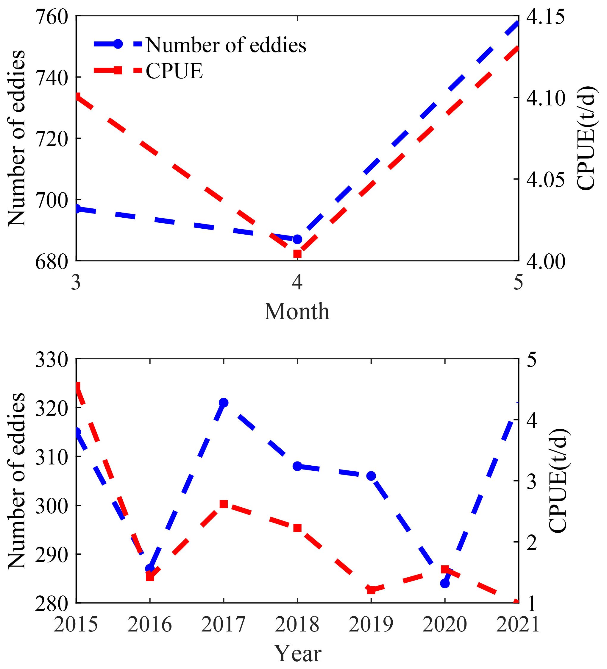
Figure 3. Monthly and annual variations in the number of eddies and D. gigas CPUE off Chile.
The spatial distribution of D. gigas CPUE, fishing effort, and catch in eddies with different polarities exhibited distinct patterns (Figure 4). In CEs, D. gigas was mostly distributed within 0-R from the eddy center, accompanied by relatively high CPUE, fishing effort, and catch. Within R-2R, D. gigas was distributed within the northwest and southeast of the eddy center. In AEs, the distribution of D. gigas was comparatively sparse within 0-R, with lower CPUE, fishing effort, and catch, while within R-2R, D. gigas was mainly concentrated to the northeast of the eddy center. Overall, the relationship between D. gigas CPUE, fishing effort, and catch, and the distance from the eddy center revealed that both catch and fishing effort initially increased and then decreased with increasing distance from CE and AE centers. In contrast, the CPUE increased consistently with an increase in the distance from the center of CEs and AEs.
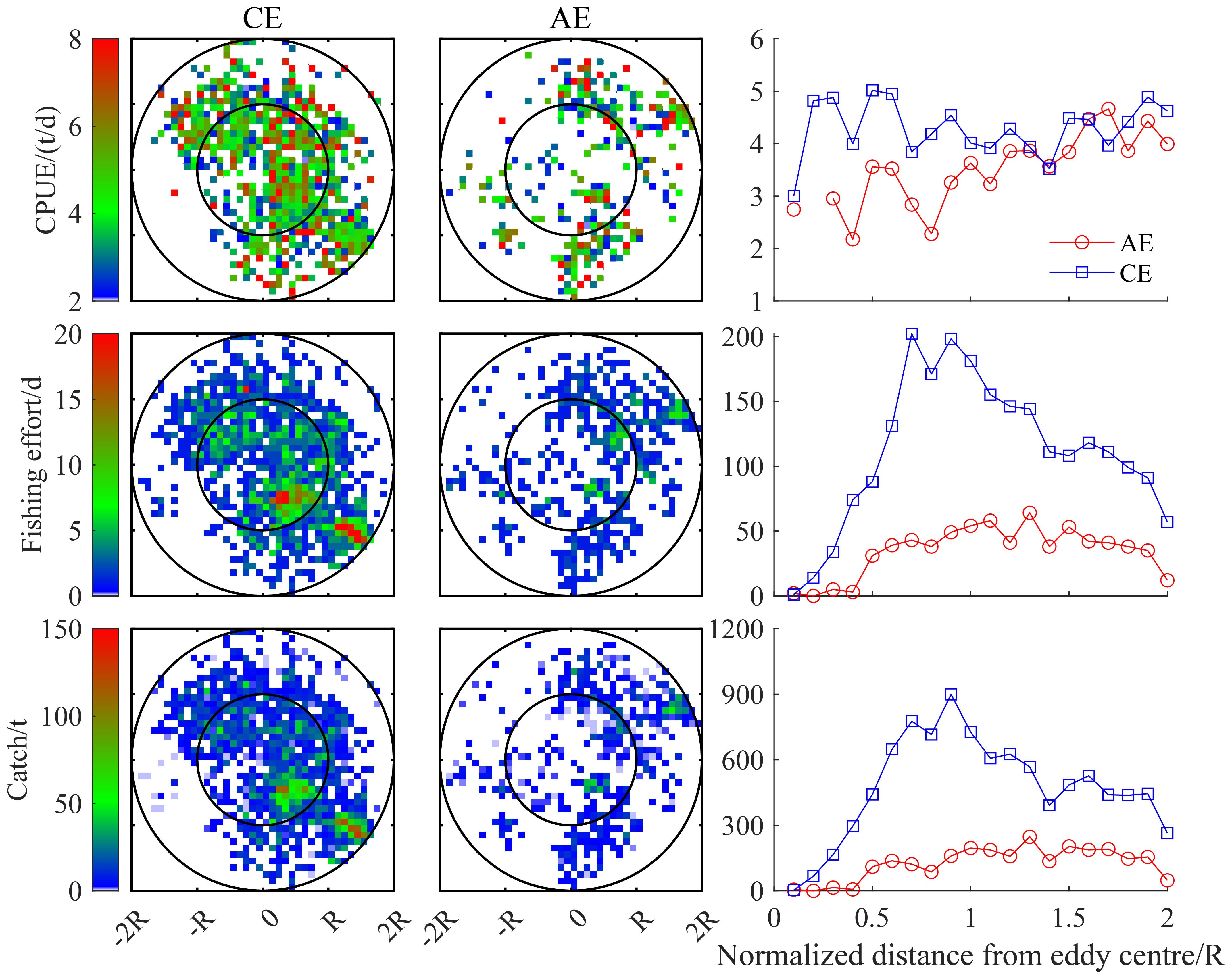
Figure 4. The spatial distribution of D. gigas CPUE, fishing effort, and catch in CEs and AEs, and their relationship with the distance from the eddy center.
GAM analysis revealed a significant correlation between the abundance of D. gigas and mesoscale eddy structures (Figure 5). The relationships between squid abundance and eddy radius or amplitude were consistently negative for both CE and AE. As the velocity of AE increased, squid abundance showed a fluctuating decreasing trend, whereas in CE, abundance first increased and then decreased with increasing velocity. With increasing eddy center longitude, squid abundance initially rose but then declined sharply. In AEs, squid abundance began to decline noticeably when the eddy center latitude reached approximately 28°S, while in CEs, the decline started around 20°S. Squid abundance was negatively correlated with distance from the center of AE. In CE, abundance increased within 0–0.5R from the eddy center, declined between 0.5R and 1.5R, and rose again from 1.5R to 2R.

Figure 5. The fitted curves of the relationships between D. gigas CPUE and six eddy parameter variables (left panel, anticyclonic eddies; right panel, cyclonic eddies).
3.3 Key environmental factors affecting D. gigas abundance off Chile
The RF model explained 32.52% of the variance. The RF analysis of selected environmental factors revealed that DO, SST, Chl-a, SSS, and TEM200 had the highest importance scores, while DO200 had the lowest (Figure 6). Among these, only DO, SST, and Chl-a had a significant impact on D. gigas CPUE (p< 0.05). Therefore, DO, SST, and Chl-a were selected as the key environmental factors for D. gigas in subsequent analyses.
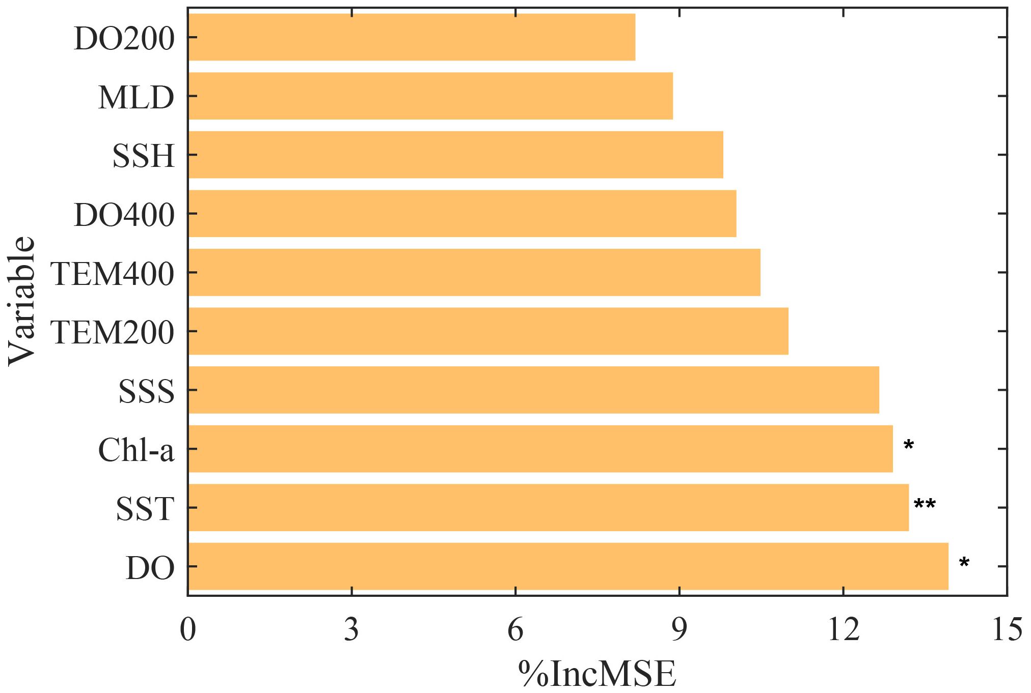
Figure 6. The importance ranking of environmental factors affecting D. gigas CPUE (significance levels: *P < 0.05 and **P < 0.01).
3.4 The distribution of key environmental factors influencing D. gigas in CEs and AEs
The distribution of fishing effort and catch within different intervals of the selected key environmental factors is presented in Figure 7. Fishing effort and catch were predominantly concentrated in the 20-21°C SST range, the 230–235 mmol/m³ (1 ml/L ≈ 44.66 mmol/m³) DO range, and the 0.1-0.15 mg/m³ Chl-a range, indicating that these are optimal ranges for D. gigas.
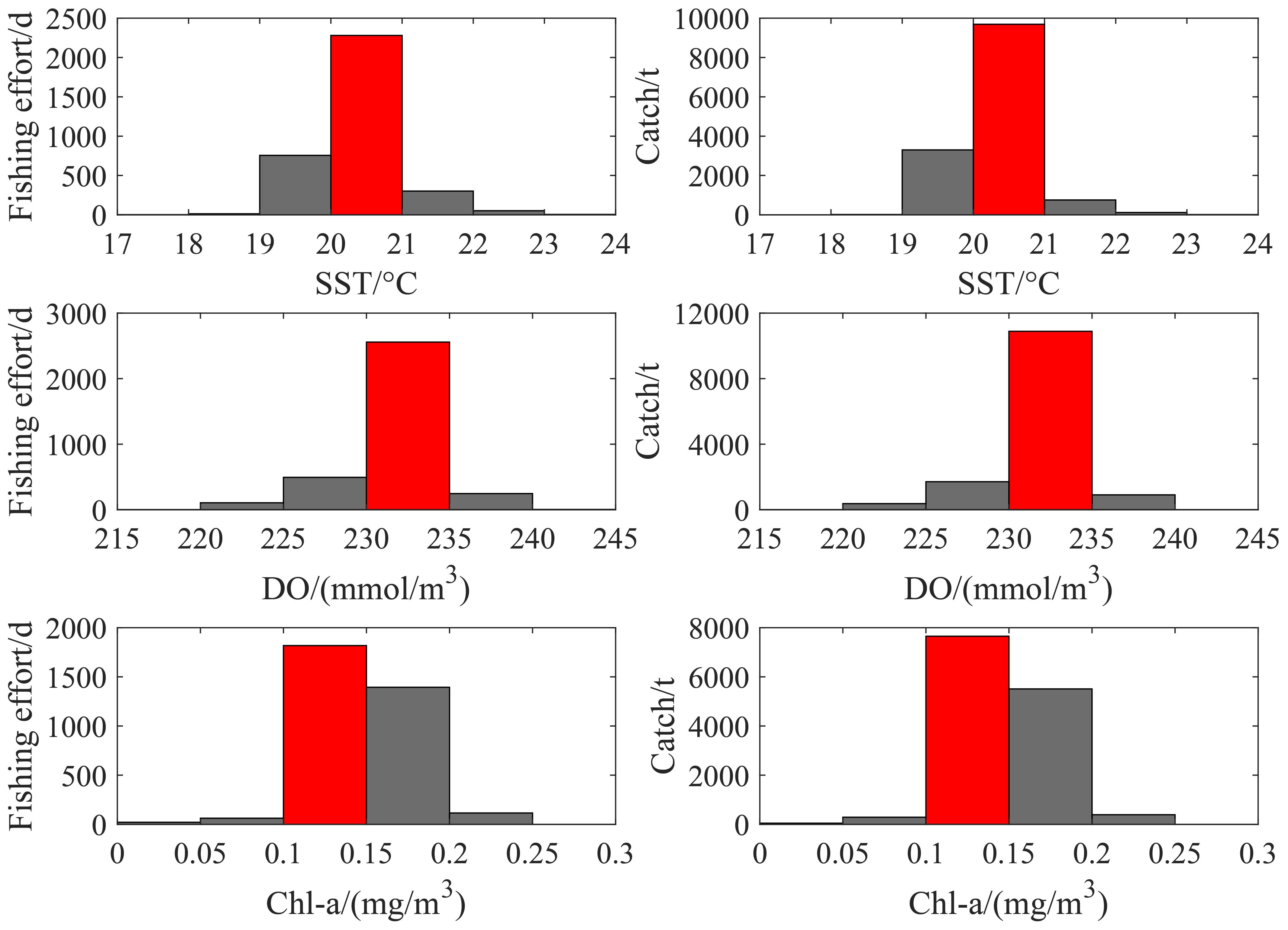
Figure 7. The distribution of fishing effort and catch in relation to different environmental factors.
The mean spatial distributions of SST, DO, and Chl-a within the 0-R range of CEs and AEs varied (Figure 8). The average spatial distribution of SST in CEs exhibited a high-to-low trend from northeast to southwest, whereas in AEs, it showed a high-to-low pattern from west to east. The average DO distribution in both types of eddies followed a north-low, south-high spatial gradient, with DO levels higher in AEs compared to CEs. The average Chl-a distribution was relatively high in both types of eddies, with Chl-a levels slightly lower in CEs than in AEs. The key environmental factors within the optimal ranges were observed more frequently in CEs than in AEs.
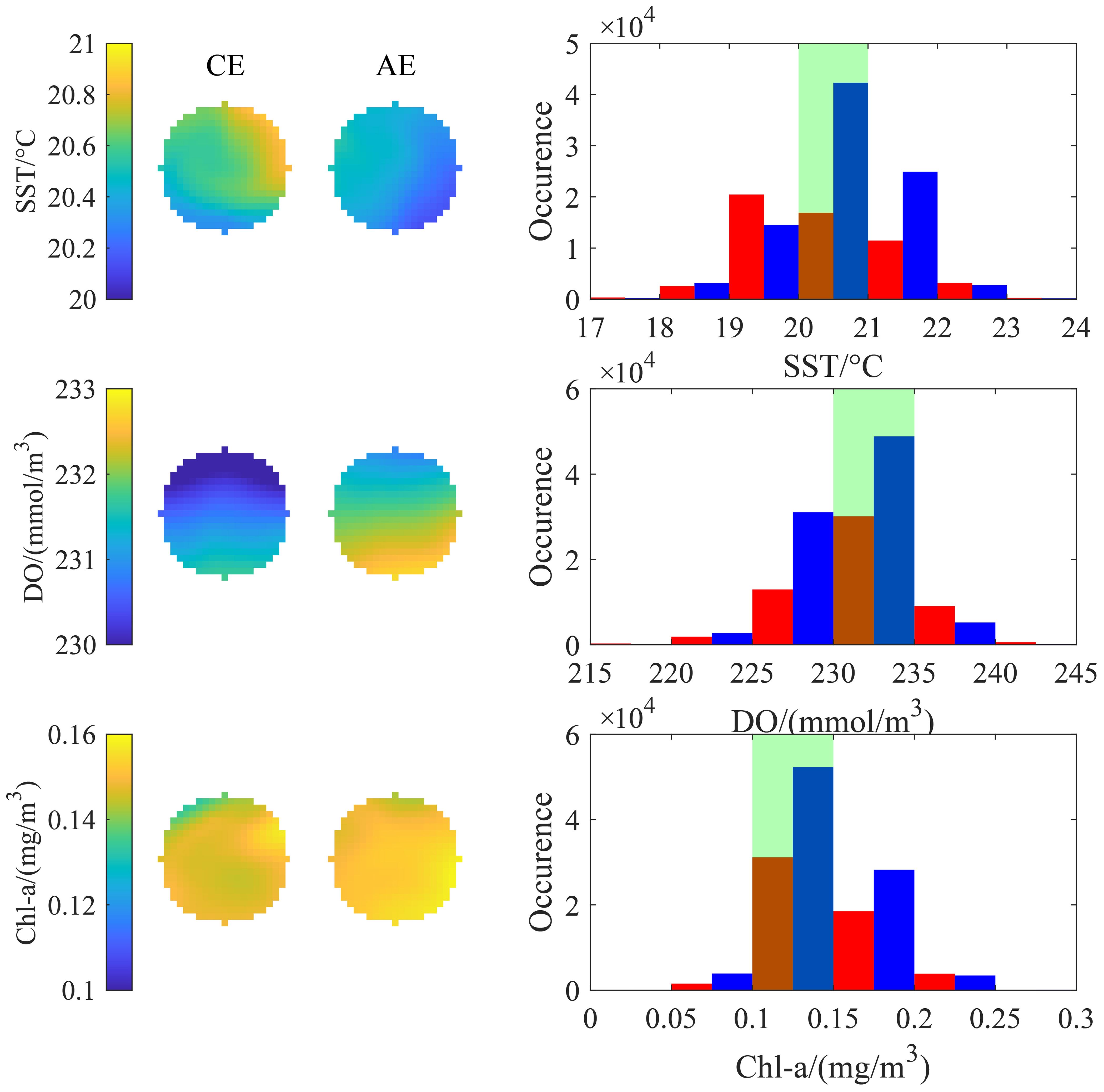
Figure 8. The mean state and histogram distribution of environmental factors within the 0-R range of eddies containing fishing operation points (blue and red bars represent CEs and AEs, respectively; green shading indicates optimal ranges of key environmental factors).
The mean spatial distributions of SST, DO, and Chl-a within the R-2R range of CEs and AEs also exhibited differences (Figure 9). Both eddy types had relatively higher SST values on the northern side of the eddy center, with higher average SST in CEs compared to AEs. For both eddy types, higher DO was primarily concentrated on the southwestern side of the eddy center, while lower DO was mainly distributed on the northern side. The average Chl-a values in CEs were relatively lower in the northwest, whereas in AEs, these were relatively lower in the northeast. The frequency of key environmental factors falling within the optimal ranges was higher in CEs compared to AEs. Additionally, the proportion of occurrences of key environmental factors within the optimal ranges was higher in CEs compared to AEs (Table 3). The greatest difference observed was the proportion of the optimal SST range between the two eddy types, with a disparity exceeding 15% in both the 0–R and R–2R ranges. For the optimal DO range, the proportions within the 0–R range of CEs and AEs were nearly identical, with a difference of less than 1%, while in the R–2R range, the disparity was approximately 3.35%. The proportion of the optimal Chl-a range was the highest, reaching up to 59.43%, although the difference between the two eddy types was relatively small.
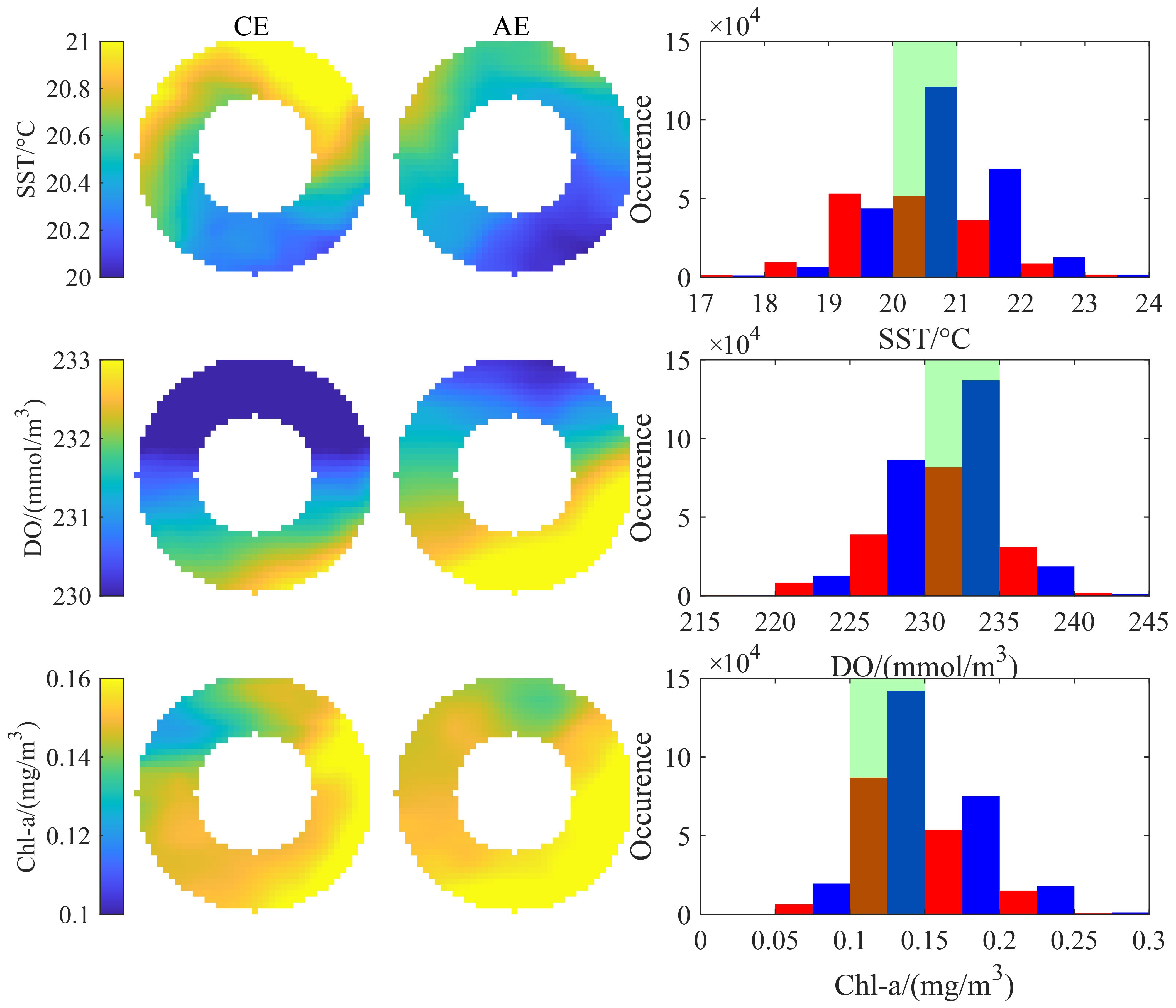
Figure 9. The mean state and histogram distribution of environmental factors within the R-2R range of eddies containing fishing operation points (blue and red bars represent CEs and AEs, respectively; green shading indicates optimal ranges of key environmental factors).
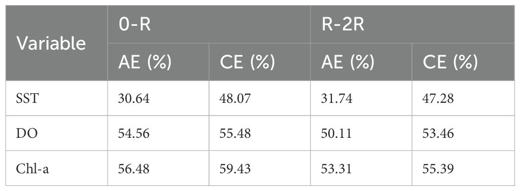
Table 3. Proportion of occurrences of key environmental factors within the optimal ranges for D. gigas in eddies, expressed as a percentage of the total occurrences in the respective range.
4 Discussion
Mesoscale eddies within eastern boundary upwelling systems are highly active, with the mechanisms of eddy formation varying across regions (Chaigneau et al., 2009). A numerical simulation study of the current systems off Chile revealed that eddy formation in this area was primarily driven by unstable coastal currents and wind stress (Hormazabal et al., 2004). Based on a global eddy dataset, this study found that mesoscale eddies in Chilean waters are predominantly generated in coastal regions (Figure 2), and they propagate westward (Figures 1E, F), aligning with previous research findings (Chaigneau et al., 2009; Chaigneau and Pizarro, 2005). However, this study identified that most eddies propagate toward the equator, whereas earlier studies (Chelton et al., 2007) indicated that CEs moved poleward, and AEs moved equatorward. These differences may be attributed to the different methods used to identify eddies in the two studies. Additionally, the two studies applied different lifetime thresholds to filter their eddy datasets, further contributing to the observed differences. Monthly and interannual variations in the Chilean ocean currents (Montecinos and Gomez, 2010) likely exert a significant influence on the formation, evolution, and dissipation of mesoscale eddies. By analyzing the temporal distribution of eddies based on their formation time, this study observed monthly and annual fluctuations in the number of CEs and AEs (Figures 1A–D), further corroborating this perspective. Eddies can be categorized into short-lived, medium-lived, and long-lived based on their lifetime (Chen and Han, 2019). Off Chile, most eddies were short-lived, of which most were CEs, whereas long-lived eddies accounted for only 0.58% of all eddies and were predominantly AEs (Table 2). These differences in eddy lifetimes may exert varying impacts on the abundance and distribution of D. gigas.
The abundance of D. gigas showed monthly and annual positive correlations with the number of eddies (Figure 3). Beyond eddy numbers, characteristics such as the amplitude, eddy kinetic energy (EKE), and life stages have been shown to influence the distribution and abundance of marine species to varying degrees (Alabia et al., 2015; Chambault et al., 2019; Xing et al., 2023). For example, in the southwest Atlantic Ocean, the abundance of Argentine shortfin squid was highly correlated with EKE during their northward migration from March to May, the primary fishing season (Ko et al., 2024). Consistently, this study revealed significant correlations between the abundance of D. gigas at different fishing locations and mesoscale eddy structural features—including radius, velocity, amplitude, eddy center longitude and latitude, and distance to the eddy center (Figure 5). Both CEs and AEs redistribute the surrounding seawater and its productivity through various physical processes during their movement (McGillicuddy, 2016). CEs generate upwelling at their centers, transporting nutrient-rich deep water to the surface, creating favorable conditions for phytoplankton blooms. This, in turn, attracts zooplankton and small fish, providing abundant food resources for higher trophic levels and forming regions of high productivity (Bailleul et al., 2010; Dragon et al., 2010; Garcia et al., 2022; Matis et al., 2014). Through analyzing the spatial distribution of D. gigas relative to eddy centers, this study found that D. gigas abundance in the 0–R and R–2R regions of CEs was consistently higher than that in AEs, with a more pronounced difference in the 0–R region. Additionally, fishing activity was more concentrated within CEs (Figure 4). These findings further validate the notion that CEs enhance productivity, benefiting marine ecosystems.
In this study, SST, Chl-a, and DO significantly influenced the abundance of D. gigas off Chile (Figure 6). From March to May, the optimal SST range for D. gigas in this region was 20–21°C (Figure 7), similar to that in Peru (20–26°C) (Yu et al., 2016), and in contrast to that in the equatorial Pacific Ocean (25–26.8°C) (Wen et al., 2024) during the same period. Comparing the optimal SST ranges across the three regions, it is evident that the D. gigas off Chile favor the lowest SST range, likely due to the latitudinal differences. SST decreases from low to high latitudes, and the waters off Chile are situated at the highest latitude, resulting in a lower SST compared to the other two regions. From March to May, the optimal Chl-a range for D. gigas off Chile was 0.1–0.15 mg/m³ (Figure 7). By comparison, this was 0.15–0.18 mg/m³ in the equatorial Pacific Ocean (Wen et al., 2024) and 0.07–0.27 mg/m³ off Peru (Yu et al., 2016). Variations in predation pressure across regions may account for these differences in the optimal Chl-a range. Previous research found that D. gigas off the northern Californian coast is more frequently observed at a depth of 30 m where DO ranges from 3.0–4.5 ml/L (Chesney et al., 2013). In contrast, this study revealed that the optimal DO range for D. gigas off Chile was 230–235 mmol/m³ (Figure 7). This suggests that D. gigas may exhibit specific preferences for DO levels at different water depths.
SST is considered one of the key environmental factors closely associated with changes in the abundance and distribution of D. gigas in their fishing grounds (Robinson et al., 2013; Waluda and Rodhouse, 2006; Wen et al., 2024). Waters rich in Chl-a provide favorable feeding grounds for D. gigas (Ichii et al., 2002), and previous studies have confirmed a link between high Chl-a regions and squid yields (Robinson et al., 2013). Seawater DO is another critical environmental factor influencing the spatial distribution of D. gigas. During the day, D. gigas typically inhabits oxygen-depleted deep waters to suppress metabolism by reducing growth and feeding activities, while at night they migrate to oxygen-rich surface waters to feed (Seibel, 2013). By comparing the distribution of key environmental factors known to influence D. gigas abundance within CEs and AEs, it was observed that, both in the 0-R and the R-2R regions, the number of key environmental factors within the optimal range was consistently higher in CEs than in AEs (Figures 8 and 9). The Proportion of occurrences of key environmental factors within the optimal ranges for D. gigas in eddies also exhibited the same pattern (Table 3). This indicates that, compared to AEs, the environmental conditions (particularly SST, Chl-a, and DO) within CEs create a more favorable habitat for D. gigas, resulting in a higher abundance of D. gigas in CEs. Additionally, the difference in the proportion of key environmental factors within the optimal range was more pronounced in the 0-R region compared to the R-2R region for both CEs and AEs (Table 3). This further explains the significant difference in the abundance of D. gigas between CEs and AEs in the 0-R region. When comparing the proportions of optimal ranges for the three environmental factors within the two types of eddies, it was found that the proportion of the optimal SST range differed by over 15%, whereas the proportions of optimal DO and Chl-a ranges differed by less than 4% (Table 3). Therefore, the favorable SST conditions in CEs are likely the primary driving factor D. gigas aggregations within these CEs.
5 Conclusions
This study utilized catch data combined with mesoscale eddy and oceanic environmental data to investigate the influence of eddies on the abundance and distribution of D. gigas off Chile. This was achieved using an RF analysis, normalization methods, and frequency distribution techniques. The results indicated that, compared to AEs, CEs create more favorable environmental conditions (particularly SST, Chl-a, and DO) for the survival of D. gigas, leading to higher aggregations of the species. The optimal SST conditions in CEs appeared to be the main driver of the favorable habitats. This study only analyzed the relationship between D. gigas distribution and mesoscale eddies during the autumn (March-May) season. However, there are differences in eddy activity and marine environments across seasons, and D. gigas exhibits different life history processes in each season. These variations may lead to differences in the response of D. gigas to mesoscale eddies across different seasons, which requires further investigation in the future.
Data availability statement
The original contributions presented in the study are included in the article/supplementary material. Further inquiries can be directed to the corresponding author.
Ethics statement
Ethical approval was not required for the study involving animals in accordance with the local legislation and institutional requirements because commercial fishing data were used in this study.
Author contributions
XW: Writing – original draft, Conceptualization, Methodology, Software. PJ: Conceptualization, Methodology, Software, Writing – original draft. WY: Writing – original draft, Writing – review & editing, Conceptualization, Funding acquisition, Methodology, Software.
Funding
The author(s) declare that financial support was received for the research and/or publication of this article. This study was financially supported by the 2024 International Cooperation Seed Funding Project for China's Ocean Decade Actions (GHZZ3702840002024020000024), the AI Special Program of Shanghai Municipal Education Commission for Wei Yu in Shanghai Ocean University (A1-3405-25-000303), Shanghai talent development funding for the project (2021078), and the Natural Science Foundation of Shanghai (23ZR1427100).
Acknowledgments
Thanks to AVISO for providing the mesoscale eddy data and to CMEMS for the environmental data. All authors confirm that the following manuscript is a transparent and honest account of the reported research. This research is related to a previous study by the same authors titled Changing Humboldt squid abundance and distribution at different stages of oceanic mesoscale eddies. The previous study was performed on the effects of mesoscale eddy evolution on the abundance and distribution of D. gigas off Peru during 2019 and the current submission is focusing on response of D. gigas to different types of mesoscale eddies off Chile during March to May from 2015 to 2019. The study is following the methodology explained in previous study.
Conflict of interest
The authors declare that the research was conducted in the absence of any commercial or financial relationships that could be construed as a potential conflict of interest.
Generative AI statement
The author(s) declare that no Generative AI was used in the creation of this manuscript.
Publisher’s note
All claims expressed in this article are solely those of the authors and do not necessarily represent those of their affiliated organizations, or those of the publisher, the editors and the reviewers. Any product that may be evaluated in this article, or claim that may be made by its manufacturer, is not guaranteed or endorsed by the publisher.
References
Alabia I. D., Saitoh S.-I., Mugo R., Igarashi H., Ishikawa Y., Usui N., et al. (2015). Identifying pelagic habitat hotspots of neon flying squid in the temperate waters of the central north pacific. PLoS One 10, e0142885. doi: 10.1371/journal.pone.0142885
Arkhipkin A. I., Nigmatullin C. M., Parkyn D. C., Winter A., Csirke J. (2023). High seas fisheries: the Achilles’ heel of major straddling squid resources. Rev. Fish Biol. Fisheries. 33, 453–474. doi: 10.1007/s11160-022-09733-8
Arkhipkin A. I., Rodhouse P. G. K., Pierce G. J., Sauer W., Sakai M., Allcock L., et al. (2015). World squid fisheries. Rev. Fish. Sci. Aquac. 23, 92–252. doi: 10.1080/23308249.2015.1026226
Bailleul F., Cotte C., Guinet C. (2010). Mesoscale eddies as foraging area of a deep-diving predator, the southern elephant seal. Mar. Ecol. Prog. Ser. 408, 251–264. doi: 10.3354/meps08560
Bakun A. (2006). Fronts and eddies as key structures in the habitat of marine fish larvae: opportunity, adaptive response and competitive advantage. Sci. Mar. 70, 105–122. doi: 10.3989/scimar.2006.70s2105
Bograd S. J., Jacox M. G., Hazen E. L., Lovecchio E., Montes I., Pozo Buil M., et al. (2023). Climate change impacts on eastern boundary upwelling systems. Annu. Rev. Mar. Sci. 15, 303–328. doi: 10.1146/annurev-marine-032122-021945
Camacho C. A., Sullivan C. J., Weber M. J., Pierce C. L. (2019). Morphological identification of bighead carp, silver carp, and grass carp eggs using random forests machine learning classification. North Am. J. Fish Manage. 39, 1373–1384. doi: 10.1002/nafm.10380
Chaigneau A., Eldin G., Dewitte B. (2009). Eddy activity in the four major upwelling systems from satellite altimetry, (1992–2007). Prog. Oceanogr. 83, 117–123. doi: 10.1016/j.pocean.2009.07.012
Chaigneau A., Pizarro O. (2005). Eddy characteristics in the eastern South Pacific. J. Geophys. Res. 110, 2004JC002815. doi: 10.1029/2004JC002815
Chambault P., Baudena A., Bjorndal K. A., Santos M. A. R., Bolten A. B., Vandeperre F. (2019). Swirling in the ocean: Immature loggerhead turtles seasonally target old anticyclonic eddies at the fringe of the North Atlantic gyre. Prog. Oceanogr. 175, 345–358. doi: 10.1016/j.pocean.2019.05.005
Chavez F. P., Bertrand A., Guevara-Carrasco R., Soler P., Csirke J. (2008). The northern Humboldt Current System: Brief history, present status and a view towards the future. Prog. Oceanogr. 79 (2-4), 95–105. doi: 10.1016/j.pocean.2008.10.012
Chavez F. P., Messié M. (2009). A comparison of eastern boundary upwelling ecosystems. Prog. Oceanogr. 83, 80–96. doi: 10.1016/j.pocean.2009.07.032
Chelton D. B., Gaube P., Schlax M. G., Early J. J., Samelson R. M. (2011). The influence of nonlinear mesoscale eddies on near-surface oceanic chlorophyll. Science. 334, 328–332. doi: 10.1126/science.1208897
Chelton D. B., Schlax M. G., Samelson R. M., De Szoeke R. A. (2007). Global observations of large oceanic eddies. Geophys. Res. Lett. 34, 2007GL030812. doi: 10.1029/2007GL030812
Chen G., Han G. (2019). Contrasting short-lived with long-lived mesoscale eddies in the global ocean. JGR Oceans. 124, 3149–3167. doi: 10.1029/2019JC014983
Chen X. (2019). Development status of world cephalopod fisheries and suggestions for squid jigging fishery in China. J. shanghai ocean Univ. 28, 321–330. doi: 10.12024/jsou.20181102445
Chesney T. A., Heppell S. S., Montero J., Graham J. (2013). Interannual variability of humboldt squid (Dosidicus gigas) off Oregon and southern Washington. Calif. Coop. Ocean. Fish. Invest. Rep. 54, 180–191.
Choi Y.-K., Kim S.-W., Jeong H.-D., Shim J.-M., Kwon K.-Y. (2013). Coastal stratification induced by oceanographic conditions of open sea in the east sea on februar. Korean Soc Mar. Environ. 19, 327–333. doi: 10.7837/kosomes.2013.19.4.327
Cutler D. R., Edwards T. C., Beard K. H., Cutler A., Hess K. T. (2007). Random forests for classification in ecology. Ecology. 88, 2783–2792. doi: 10.1890/07-0539.1
Dong C., McWilliams J. C., Liu Y., Chen D. (2014). Global heat and salt transports by eddy movement. Nat. Commun. 5, 3294. doi: 10.1038/ncomms4294
Dragon A.-C., Monestiez P., Bar-Hen A., Guinet C. (2010). Linking foraging behaviour to physical oceanographic structures: Southern elephant seals and mesoscale eddies east of Kerguelen Islands. Prog. Oceanogr. 87, 61–71. doi: 10.1016/j.pocean.2010.09.025
Durán Gómez G. S., Nagai T., Yokawa K. (2020). Mesoscale warm-core eddies drive interannual modulations of swordfish catch in the kuroshio extension system. Front. Mar. Sci. 7. doi: 10.3389/fmars.2020.00680
Espinoza-Morriberón D., Echevin V., Colas F., Tam J., Ledesma J., Vásquez L., et al. (2017). Impacts of El Niño events on the Peruvian upwelling system productivity. J. Geophys. Res. 122, 5423–5444. doi: 10.1002/2016JC012439
Everingham Y., Sexton J., Skocaj D., Inman-Bamber G. (2016). Accurate prediction of sugarcane yield using a random forest algorithm. Agron. Sustain. Dev. 36, 27. doi: 10.1007/s13593-016-0364-z
Feng Z., Yu W., Chen X. (2022). Concurrent habitat fluctuations of two economically important marine species in the Southeast Pacific Ocean off Chile in relation to ENSO perturbations. Fish Oceanogr. 31, 123–134. doi: 10.1111/fog.12566
Garcia V., Schilling H., Cruz D., Hawes S., Everett J., Roughan M., et al. (2022). Entrainment and development of larval fish assemblages in two contrasting cold core eddies of the East Australian Current system. Mar. Ecol. Prog. Ser. 685, 1–18. doi: 10.3354/meps13982
Gaube P., Barceló C., McGillicuddy D. J., Domingo A., Miller P., Giffoni B., et al. (2017). The use of mesoscale eddies by juvenile loggerhead sea turtles (Caretta caretta) in the southwestern Atlantic. PLoS One 12, e0172839. doi: 10.1371/journal.pone.0172839
Gaube P., Braun C. D., Lawson G. L., McGillicuddy D. J., Penna A. D., Skomal G. B., et al. (2018). Mesoscale eddies influence the movements of mature female white sharks in the Gulf Stream and Sargasso Sea. Sci. Rep. 8, 7363. doi: 10.1038/s41598-018-25565-8
Giamalaki K., Beaulieu C., Prochaska J. X. (2022). Assessing predictability of marine heatwaves with random forests. Geophys. Res. Lett. 49, e2022GL099069. doi: 10.1029/2022GL099069
Gonzalez-Pestana A., Alfaro-Shigueto J., Mangel J. C. (2022). A review of high trophic predator-prey relationships in the pelagic Northern Humboldt system, with a focus on anchovetas. Fish Oceanogr. 253, 106386. doi: 10.1016/j.fishres.2022.106386
Gutiérrez D., Akester M., Naranjo L. (2016). Productivity and Sustainable Management of the Humboldt Current Large Marine Ecosystem under climate change. Environ. Dev. 17, 126–144. doi: 10.1016/j.envdev.2015.11.004
Hormazabal S., Shaffer G., Leth O. (2004). Coastal transition zone off Chile. J. Geophys. Res. 109 (C1), 1–13. doi: 10.1029/2003JC001956
Hsu A. C., Boustany A. M., Roberts J. J., Chang J., Halpin P. N. (2015). Tuna and swordfish catch in the U.S. northwest Atlantic longline fishery in relation to mesoscale eddies. Fish Oceanogr. 24, 508–520. doi: 10.1111/fog.12125
Ibáñez C. M., Sepúlveda R. D., Ulloa P., Keyl F., Pardo-Gandarillas M. C. (2016). The biology and ecology of the jumbo squid Dosidicus gigas (Cephalopoda) in Chilean waters: a review. Lat. Am. J. Aquat. Res. 43, 402–414. doi: 10.3856/vol43-issue3-fulltext-2
Ichii T., Mahapatra K., Watanabe T., Yatsu A., Inagake D., Okada Y. (2002). Occurrence of jumbo flying squid Dosidicus gigas aggregations associated with the countercurrent ridge off the Costa Rica Dome during 1997 El Niño and 1999 La Niña. Mar. Ecol. Prog. Ser. 231, 151–166. doi: 10.3354/meps231151
Jersild A., Delawalla S., Ito T. (2021). Mesoscale eddies regulate seasonal iron supply and carbon drawdown in the drake passage. Geophys. Res. Lett. 48, e2021GL096020. doi: 10.1029/2021GL096020
Jian Y. J., Zhang J., Liu Q. S., Wang Y. F. (2009). Effect of Mesoscale eddies on underwater sound propagation. Appl. Acoust. 70, 432–440. doi: 10.1016/j.apacoust.2008.05.007
Jin P., Zhang Y., Du Y., Chen X., Kindong R., Xue H., et al. (2024). Eddy impacts on abundance and habitat distribution of a large predatory squid off Peru. Mar. Environ. Res. 195, 106368. doi: 10.1016/j.marenvres.2024.106368
Keith D. A., Ferrer-Paris J. R., Nicholson E., Kingsford R. T. (2020). IUCN Global Ecosystem Typology 2.0. Gland, CH: International Union For Conservation of Nature.
Ko C.-Y., Lee Y.-C., Wang Y.-C., Hsu H.-H., Chow C. H., Chen R.-G., et al. (2024). Modulations of ocean-atmosphere interactions on squid abundance over Southwest Atlantic. Environ. Res. 250, 118444. doi: 10.1016/j.envres.2024.118444
Mariano Gutiérrez T., Jorge Castillo P., Laura Naranjo B., Akester M. J. (2017). Current state of goods, services and governance of the Humboldt Current Large Marine Ecosystem in the context of climate change. Environ. Dev. 22, 175–190. doi: 10.1016/j.envdev.2017.02.006
Markaida U. (2006). Food and feeding of jumbo squid Dosidicus gigas in the Gulf of California and adjacent waters after the 1997–98 El Niño event. Fish Res. 79, 16–27. doi: 10.1016/j.fishres.2006.02.016
Matis P. A., Figueira W. F., Suthers I. M., Humphries J., Miskiewicz A., Coleman R. A., et al. (2014). Cyclonic entrainment? The ichthyoplankton attributes of three major water mass types generated by the separation of the East Australian Current. ICES J. Mar. Sci. 71, 1696–1705. doi: 10.1093/icesjms/fsu062
McGillicuddy D. J. (2016). Mechanisms of physical-biological-biogeochemical interaction at the oceanic mesoscale. Annu. Rev. Mar. Sci. 8, 125–159. doi: 10.1146/annurev-marine-010814-015606
Montecinos A., Gomez F. (2010). ENSO modulation of the upwelling season off southern-central Chile. Geophys. Res. Lett. 37, 2009GL041739. doi: 10.1029/2009GL041739
Nigmatullin C. (2001). A review of the biology of the jumbo squid Dosidicus gigas (Cephalopoda: Ommastrephidae). Fish Res. 54, 9–19. doi: 10.1016/S0165-7836(01)00371-X
O’brien R. M. (2007). A caution regarding rules of thumb for variance inflation factors. Qual Quant. 41, 673–690. doi: 10.1007/s11135-006-9018-6
Pegliasco C., Delepoulle A., Mason E., Morrow R., Faugère Y., Dibarboure G. (2022). META3.1exp: a new global mesoscale eddy trajectory atlas derived from altimetry. Earth Syst. Sci. Data. 14, 1087–1107. doi: 10.5194/essd-14-1087-2022
Portner E. J., Markaida U., Robinson C. J., Gilly W. F. (2020). Trophic ecology of Humboldt squid, Dosidicus gigas, in conjunction with body size and climatic variability in the Gulf of California, Mexico. Limnol. Oceanogr. 65, 732–748. doi: 10.1002/lno.11343
Prasad A. M., Iverson L. R., Liaw A. (2006). Newer classification and regression tree techniques: bagging and random forests for ecological prediction. Ecosystems. 9, 181–199. doi: 10.1007/s10021-005-0054-1
Probst P., Wright M., Boulesteix A.-L. (2019). Hyperparameters and tuning strategies for random forest. WIREs Data Min Knowl. 9, e1301. doi: 10.1002/widm.1301
Receveur A., Menkes C., Lengaigne M., Ariza A., Bertrand A., Dutheil C., et al. (2024). A rare oasis effect for forage fauna in oceanic eddies at the global scale. Nat. Commun. 15, 4834. doi: 10.1038/s41467-024-49113-3
Robinson C. J., Gomez-Gutierrez J., Salas de Leon D. A. (2013). Jumbo squid (Dosidicus gigas) landings in the Gulf of California related to remotely sensed SST and concentrations of chlorophylla, (1998-2012). Fish Res. 137, 97–103. doi: 10.1016/j.fishres.2012.09.006
Sakai M., Tsuchiya K., MARIATEGUI L., Wakabayashi T., Yamashiro C. (2017). Vertical Migratory Behavior of Jumbo Flying Squid (Dosidicus gigas) off Peru: Records of Acoustic and Pop-up Tags. Jpn. Agric. Res. Q. 51, 171–179. doi: 10.6090/jarq.51.171
Sandoval-Castellanos E., Uribe-Alcocer M., Díaz-Jaimes P. (2007). Population genetic structure of jumbo squid (Dosidicus gigas) evaluated by RAPD analysis. Fish Res. 83, 113–118. doi: 10.1016/j.fishres.2006.09.007
Seibel B. A. (2013). The jumbo squid, Dosidicus gigas (Ommastrephidae), living in oxygen minimum zones II: Blood–oxygen binding. Deep Sea Res. Part II Top. Stud. Oceanogr. 95, 139–144. doi: 10.1016/j.dsr2.2012.10.003
Thiel M., Macaya E., Acuña E., Arntz W. (2007). The humboldt current system of northern and central Chile: Oceanographic processes, ecological interactions and socioeconomic feedback. Oceanogr. Mar. Biol. Annu. Rev. 45, 195–344. doi: 10.1201/9781420050943.ch6
Waluda C. M., Rodhouse P. G. (2006). Remotely sensed mesoscale oceanography of the Central Eastern Pacific and recruitment variability in. Dosidicus gigas. Mar. Ecol.-Prog. Ser. 310, 25–32. doi: 10.3354/meps310025
Wang H., Qiu B., Liu H., Zhang Z. (2023). Doubling of surface oceanic meridional heat transport by non-symmetry of mesoscale eddies. Nat. Commun. 14, 5460. doi: 10.1038/s41467-023-41294-7
Watanabe H., Kubodera T., Moku M., Kawaguchi K. (2006). Diel vertical migration of squid in the warm core ring and cold water masses in the transition region of the western North Pacific. Mar. Ecol. Prog. Ser. 315, 187–197. doi: 10.3354/meps315187
Wen J., Zhou Z., Zhang Y., Yu W., Chen B., Chen X. (2024). Climate-related habitat variations of Humboldt squid in the eastern equatorial Pacific Ocean. J. Mar Syst. 243, 103960. doi: 10.1016/j.jmarsys.2023.103960
Wood S. M. (2006). Generalized Additive Models, an Introduction with R (London, UK: Chapman and Hall).
Wu X., Jin P., Zhang Y., Yu W. (2024). Spatial distribution and abundance of a pelagic squid during the evolution of eddies in the Southeast Pacific Ocean. JMSE. 12, 1015. doi: 10.3390/jmse12061015
Xing Q., Yu H., Wang H., Ito S., Chai F. (2023). Mesoscale eddies modulate the dynamics of human fishing activities in the global midlatitude ocean. FISH FISH. 24, 527–543. doi: 10.1111/faf.12742
Xing Q., Yu H., Wang H., Ito S., Yu W. (2024). Mesoscale eddies exert inverse latitudinal effects on global industrial squid fisheries. Sci. Total Environ. 950, 175211. doi: 10.1016/j.scitotenv.2024.175211
Yu W., Yi Q., Chen X., Chen Y. (2016). Modelling the effects of climate variability on habitat suitability of jumbo flying squid, Dosidicus gigas, in the Southeast Pacific Ocean off Peru. ICES J. Mar. Sci. 73, 239–249. doi: 10.1093/icesjms/fsv223
Yun J., Ha K.-J., Lee S.-S. (2024). Impact of greenhouse warming on mesoscale eddy characteristics in high-resolution climate simulations. Environ. Res. Lett. 19, 014078. doi: 10.1088/1748-9326/ad114b
Keywords: Dosidicus gigas, mesoscale eddies, environmental change, abundance, Chile
Citation: Wu X, Jin P and Yu W (2025) The relationship between mesoscale eddies and the abundance and distribution of jumbo flying squid off Chile. Front. Mar. Sci. 12:1575299. doi: 10.3389/fmars.2025.1575299
Received: 12 February 2025; Accepted: 14 April 2025;
Published: 08 May 2025.
Edited by:
Giuseppe Suaria, National Research Council, ItalyReviewed by:
Daniel B. Lluch-Cota, Centro de Investigaciones Biológicas del Noroeste S.C., MexicoYang Zhang, Ministry of Natural Resources, China
Copyright © 2025 Wu, Jin and Yu. This is an open-access article distributed under the terms of the Creative Commons Attribution License (CC BY). The use, distribution or reproduction in other forums is permitted, provided the original author(s) and the copyright owner(s) are credited and that the original publication in this journal is cited, in accordance with accepted academic practice. No use, distribution or reproduction is permitted which does not comply with these terms.
*Correspondence: Wei Yu, d3l1QHNob3UuZWR1LmNu