High-precision refraction correction of ICESat-2 bathymetry based on sea-wave profiles with a piece-point polynomial model

The Ice, Cloud, and Land Elevation Satellite-2 (ICESat-2), featuring the advanced topographic laser altimeter system (ATLAS), pioneered spaceborne photon-counting LiDAR technology. The first spaceborne laser system in Earth’s orbit with water detection capabilities, offers a more direct approach for charting the bathymetry and underwater topography in coastal waters. However, the refraction effect of water column on light is not taken into account by ATLAS products, which will cause the position change of signal photons on the seafloor, consequently reducing the precision of nearshore bathymetry and underwater topography mapping. In the previous studies, the fluctuation water surface has been assumed as the plane to achieve the water refraction correction. In this process, the water incident angle, refraction angle and water refraction direction are same for all seafloor photons, which decreases the accuracy of the photon position and the nearshore bathymetry. Therefore, we present an innovative method for addressing refraction correction by tracking the trajectory of individual photons on the seafloor and reconstructing sea-wave profiles to achieve high-accuracy refraction correction for ATLAS data. In this method, the instantaneous sea wave has been modeled using the extracted signal photon of water surface and the proposed weight cubic polynomial model. Further, the corresponding various incident and refraction angles of each seafloor photon were accurately obtained to calculate various the displacement quantity and direction. Moreover, a coordinate correction model was introduced to aim at enhancing the accuracy of photon coordinates on the seafloor and mapping of underwater topography. Validation results demonstrate that the proposed method for refraction correction effectively enhances the bathymetric precision. The maximum depth displacement corrected in the study area reached 5.46 m, occurring at a water depth of 16.01 m. In the along-track direction, there was a range of maximum displacements from -0.54 to 0.47 m, while the maximum relative displacement reached 1.01 m, significantly exceeding the displacement observed in the cross-track direction.

1 Introduction

The Ice, Cloud, and Land Elevation Satellite-2 (ICESat-2) incorporates an innovative topographic laser altimeter system (ATLAS), offering a unique method for precisely assessment of changes on the Earth’s surface (Neuenschwander et al., 2020). The ICESat-2 mission supported by NASA aims to collect and distribute data for various scientific fields, including monitoring changes in elevation of mountain glaciers and ice caps, measuring heights of land and vegetation, evaluating inland water elevations, recording sea surface heights, and observing cloud layering patterns (Shang et al., 2022). ATLAS is the first spaceborne laser altimeter employing a photon-counting technique, utilizing green laser light with the wavelength of 532 nm. The laser pulse is emitted at a rate of 10,000 times per second (10,000 Hz), as well as the energy of each pulse was approximately 0.12 mJ, resulting in a small footprint of 17 meters in diameter and a sampling interval along the track of 0.7 m (Dietrich et al., 2024). Owing to the use of green laser light, ATLAS provides the unique opportunity to achieve active remote-sensing bathymetry and underwater topography in nearshore areas (Yang et al., 2022; Xie et al., 2023; Le et al., 2022; Wu et al., 2024).

Nearshore bathymetry is a crucial research topic that is notoriously difficult to perform, particularly for those islands and coastlines far away from the mainland (Albright and Glennie, 2020; Salameh et al., 2019). Currently, existing methods (e.g., satellite derived bathymetry (SDB) airborne LiDAR bathymetric system (ALB) and shipborne multi-beam sonar system) are easily limited by various factors (Kim et al., 2014; Jawak et al., 2015; Xu et al., 2021; Yang et al., 2022), such as the acquisition of in situ data, spatiotemporal conditions, bathymetric resolution, and regional environment. ATLAS offers a more direct approach for bathymetric mapping, effectively addressing several existing limitations (Li et al., 2019; Xu et al., 2024). In a bathymetric process utilizing a method of photon-counting, it is necessary to detect photons that are dispersed across various spatial regions, including water surface and underwater (Xie et al., 2021; Bernardis et al., 2023). The signal photons, describing the seafloor topography, are detected and extracted from the underwater photons whose spatial density distribution changes with increasing water depth. The nearshore bathymetry and underwater topography can be measured and obtained by the geolocated coordinates of the detected seafloor photons (Ludeno et al., 2024; Cao et al., 2023; Zhong et al., 2023). However, the refraction effects, where photons change direction and speed as they pass from one medium to another, such as from air to water, were not considered. This phenomenon, along with the decrease in photon velocity in water (~225,000 km/s), resulted in a decrement of accuracy in the bathymetry of coastal areas (Zhang et al., 2022; Chen et al., 2021b).

The refraction effect and reduced velocity of photons in water have a significant influence on the nearshore bathymetry with LiDAR (Xu et al., 2021). It is imperative to correct the impacts of water refraction and the decreased velocity. This correction involves considering the refraction of individual photons as they traverse the aquatic medium and engage with the seafloor, employing Snell’s principle. However, these methods are only suitable for large laser divergence angles, where multiple wave cycles are covered by a large footprint and the wave effects are averaged (Westfeld et al., 2016; Yang et al., 2017). The instantaneous geometry of the sea surface should be precisely considered and determined for a bathymetric LiDAR system with a footprint that is generally smaller than the sea swell wavelength, which leads to significant underwater point displacement with increasing water depth (Saylam et al., 2018; Mandlburger et al., 2015). Tulldahl and Westfeld (Tulldahl and Steinvall, 2004) investigated the impact of refraction on the point accuracy of ALB systems by analyzing the spatial geometric correlation between the laser beam and its alignment with the angle at which it encounters the sea surface.

For ATLAS, the bathymetric mechanism is based on the probability detection of an underwater photon event, which is completely different from the full-waveform ALB (Leng et al., 2023). Each seafloor photon has a corresponding sea surface incident point, where the laser pulse intersects with the sea wave. Precisely determining the spatial location of this intersection point for each seafloor photon and obtaining a high-accuracy instantaneous sea-wave profile are difficult. Therefore, the currently proposed and adopted refraction correction methods are relatively simple and not rigorous. These methods typically assume the sea surface to be planar or simplified as a fluctuating plane (Parrish et al., 2019). The sea-wave profile, precision incident angle, and refraction angle of each seafloor photon were not completely considered (Ma et al., 2020). Additionally, the refractive displacement affected by sea waves has a complex geometric relationship with different pointing angles for the laser pulse, sea-wave height, and water depth (Chen et al., 2021b). Therefore, challenges emerge when attempting to tackle refraction and account for the specific displacement of photons from the seafloor in coordinate terms.

To overcome these problems, a novel refraction correction method is proposed, which involves ray tracing, a technique that simulates the path of photons as they travel through different media by calculating the changes in their direction and speed for each seafloor photon. Besides, the method reconstructs the sea wave profile to achieve high-accuracy refraction correction and nearshore bathymetry for ICESat-2. In this method, the instantaneous sea wave has been modeled using the extracted signal photon of water surface and the proposed weight cubic polynomial model. The rigorous space geometry relation of laser pulse penetrating the air-water interface of sea wave to the seafloor was established. The intersection point on the air-water interface of each seafloor photon can be accurately calculated using the instantaneous sea wave and photon emission angle. The corresponding various incident and refraction angles were accurately obtained to calculate various the displacement quantity and direction for the different seafloor photon. Therefore, the absolute and relative positions accuracy of the seafloor signal photon has been improved, which further increases the nearshore bathymetry and underwater topography. Therefore, the absolute and relative positions accuracy of the seafloor signal photon has been improved, which further increases the nearshore bathymetry and underwater topography. Additionally, a coordinate correction model for each seafloor photon is proposed to correct and obtain high-accuracy coordinates of the seafloor photons and underwater topography. Finally, various experiments are carried out to validate the suggested approach and estimate its accuracy and reliability.

2 Study area and dataset

2.1 Study area

The South China Sea, located south of China’s mainland, includes archipelagos such as Dongsha, Xisha, Zhongsha, and Nansha. It is categorized as one of China’s three marginal seas. Our study area Qilianyu Islands was located at the Xisha archipelago at 16.956° N, 112.318° E. It comprised several tiny islands, sand cays, and coral reefs. Figure 1 illustrates an image of the Qilianyu Islands, indicating their position through a red circle and an orange-dashed rectangle.

Figure 1

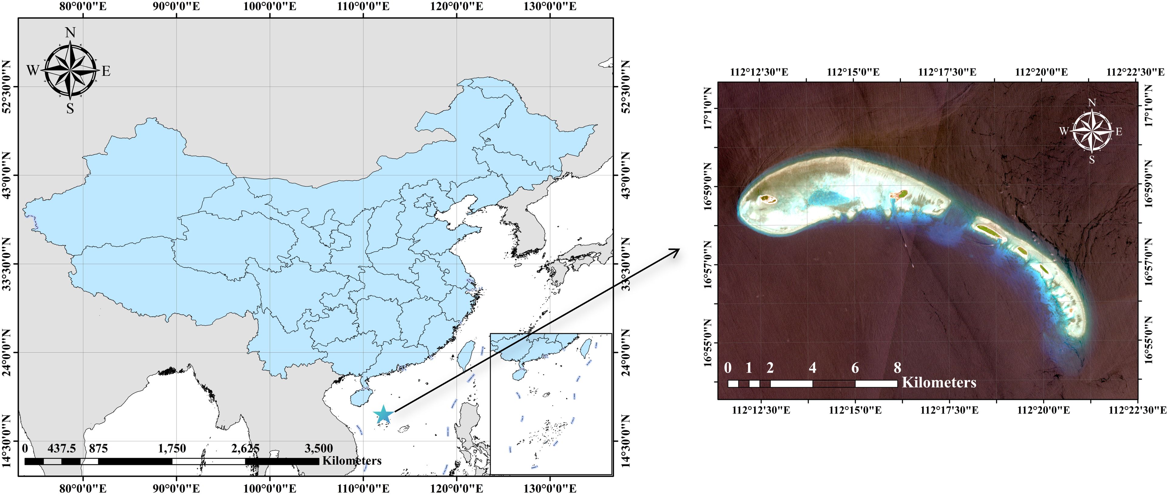
Figure 1. The image highlights the Qilianyu Islands as the study area, which is represented by a blue pentagram.

2.2 ATLAS dataset

In the study area, we utilized eight ground tracks illustrated in Figure 2a, which are included in four ATL03 products. The ATL03 product is the Level-2 Global Geolocated Photon Data from ATLAS/ICESat-2, distributed in the standard HDF-5 format. This dataset provides precise geolocation information for each detected photon, including timestamp, elevation, and latitude/longitude coordinates referenced to the WGS-84 ellipsoid (Smith et al., 2019; Neumann et al., 2019). The data is organized into six ground track groups (“gtx”), corresponding to three strong and three weak laser beams. These tracks are plotted by dashed lines of various colors. The scanning tracks of two pairs of weak and strong laser beams, shown in blue and red, respectively, which overpass the Xisha Shoal in the islands of the study area. Table 1 lists the details for all the eight groud tracks, including the acquisition time, the range of geodetic coordinates, and the density distribution of photons.

Figure 2

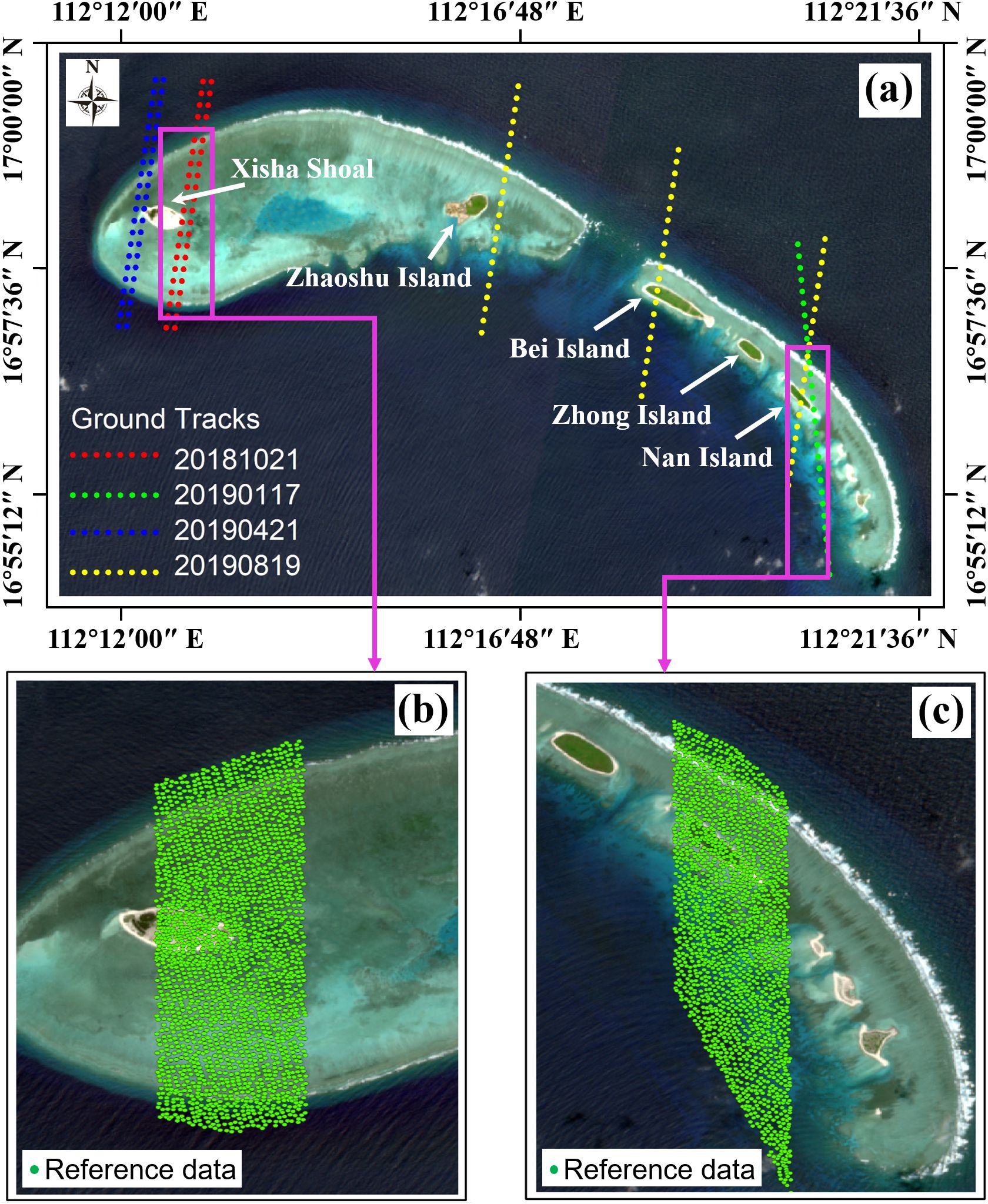
Figure 2. ATL03 datasets of eight ground tracks and the in situ data for the bathymetry are obtained for the study area, shown in (a-c), respectively.

Table 1

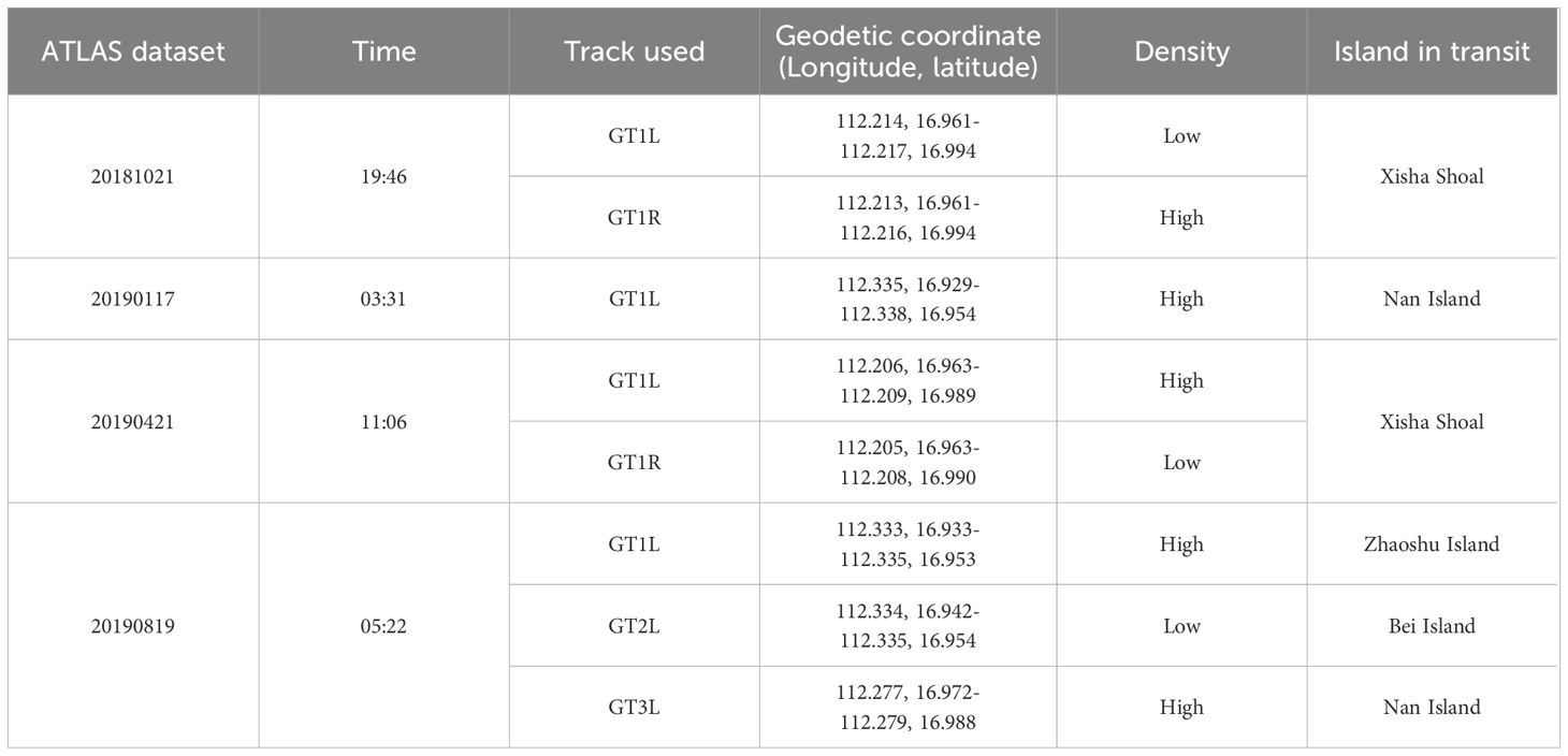
Table 1. Study sites, acquisition times, geodetic coordinates, and photon density distribution of the ATLAS datasets.

2.3 In-situ data

The in-situ data acquired by the Mapper-5000 was used to validate the accuracy of the proposed algorithm. Mapper-5000 was a dual-band ALB system developed by the Shanghai Institute of Optics and Fine Mechanics, and the nominally bathymetric accuracy of Mapper-5000 is approximately 0.2m at Xisha Islands (Liu et al., 2018). The density of the in-situ data was 0.83 points/m², as well as the distribution of these bathymetric points was illustrated in Figures 2b and 2c. The in-situ data was obtained on September 27, 2017, therefore, the tidal correction must be conducted to minimize the errors caused by the inconsistent of the acquisition time between the ICESat-2 tracks and the in-situ data (Hsu et al., 2021). In this research, the long-term tidal data was acquired from the Sansha tide gauge station, and the in-situ datasets was tidal corrected to consistent with the specific ICESat-2 ground tracks. The time resolution of long-term the tidal data was first resampled from 1 h to 1 min, and variations in the tides among the ICESat-2 and ALB data were acquired (Le et al., 2021). Finally, the elevation of the water-surface for ALB data was adjusted to consist with the water surface elevation of the ICESat-2 data.

3 Methodology

To precisely correct the displacement of each seafloor photon caused by water refraction and the velocity change of photons in water, ray tracing of each seafloor photon was performed to reconstruct the local sea-wave profile using the sea-surface photon and piece-point with the weight cubic polynomial (PWCP) model. ATLAS uses green laser light (532 nm), at 10,000 pulses per second (10 kHz), with a footprint diameter of 17 m, and along-track sampling interval of 0.7 m (Smith et al., 2019). In ATLAS, the transmit laser pulse is split into three pairs of beams to improve the data acquisition efficiency. In ATLAS, the transmit laser pulse is split into three pairs of beams to improve the data acquisition efficiency (Neumann et al., 2019). Each pair consists of a strong and weak beam and is separated by a cross-track of approximately 3 km, with pair spacing of 90 m (Markus et al., 2017). The laser pulse reaches the sea surface and penetrates the air-water interface of sea wave to the seafloor. The intersection points and slope at the air/sea interface for each seafloor photon were precisely determined by utilizing the reconstructed local sea-wave profile and transmission path obtained by ray tracing. Subsequently, a model for correction in both along- and cross-track directions was developed. This model was derived from the scanning mechanism of ATLAS, the Snell principle, and the spatial geometric relationship among the sea-wave profile, seafloor photons, and their transmission paths. Finally, the displacement resulting from water refraction was projected onto the WGS-84 ellipsoid to perform coordinate correction for each seafloor photon. The flow chart of the proposed method is shown in Figure 3.

Figure 3

Figure 3. Flow chart of refraction and coordinate correction method based on PWCP.

This method was chosen due to the complexity of accurately mapping nearshore bathymetry, where traditional approaches fall short in accounting for the effects of water refraction and dynamic sea surfaces. By using ray tracing, the method precisely simulates photon paths and reconstructs the local sea-wave profile. The incorporation of the PWCP model, Snell’s law, and spatial geometry ensures accurate corrections, making it well-suited for the ICESat-2 mission. The final projection onto the WGS-84 ellipsoid ensures globally consistent coordinate correction, providing a robust solution for high-precision coastal mapping. Therefore, comparing to the previous methods, the novel can effectively ensure the absolute and relative positions of the seafloor signal photon and improve the nearshore bathymetrical and underwater topographical accuracy.

3.1 Calculation of air/sea intersection point

The linear scanning structure of ATLAS is illustrated in Figure 4a. The x, y, and z axes represent the along-track, cross-track, and elevation directions in which the coordinates of each photon can be transformed. For the ATL03 datasets acquired in the water area, signal photons were detected and separated into two groups: the sea surface and the seafloor photons. Among the detected signal photons, some are reflected by the sea surface, while others penetrate the sea surface and reach the seafloor. When a seafloor signal photon encounters the air/water interface and penetrates the seafloor, its trajectory and speed undergo modifications due to the characteristics of the water medium.

Figure 4

Figure 4. Diagram of three pairs of ground scanning tracks. (a) Each ground track contains the strong and weak laser pulse scanning. (b) Geometric relationship and distribution of the laser pulse trajectory, various photons, and sea-wave profile.

To precisely ascertain the air/sea intersection point for each seafloor photon, it is essential to employ the reconstructed local sea-wave profile (referred to as S) and track the transmission route of the seafloor photon illustrated in Figure 4b. A spatial line is determined for the laser pulse in its original path, disregarding any refraction caused by water. This is achieved by considering the positioning angle, φ, and the coordinate of each seafloor photon during ray tracing. The spatial line, depicted as the green line in Figure 4b, is mathematically formulated as Equation 1, where $(x_q,y_q,z_q)$ is the coordinate of a specific photon on the seafloor, q, and $(e_q,e_q,e_q)$ is the unit vector of the spatial line that passes through photon q. In the x direction, the laser pulse pointing angle is decomposed and described by φ_x, while the corresponding spatial line is expressed in Equation 2:

$\begin{array}{ll}\frac{x-x_q}{e_x}=\frac{y-y_q}{e_y}=\frac{z-z_q}{e_z}& (1)\end{array}$

$\begin{array}{ll}z=-\frac{1}{\tan {\phi }_x}x+z_q+\frac{x_q}{\tan {\phi }_x}& (2)\end{array}$

The local sea-wave profile was reconstructed and refined using the proposed PWCP model, which is a high-accuracy fitting with weighting factors. The PWCP is formulated using Equation 3, where symbols a_j, b_j, c_j, and d_j are the coefficients in the cubic polynomial, j is the number of seafloor photons, and the weight function is represented by w. Figure 5 illustrates the diagram of the PWCP, where point $p^{\prime }$ is the intersection of the mean sea surface, $S_0$, with the spatial line constructed by the seafloor photon, q. In the x direction, point $p^{\prime }$ is very close to point p, which is used to obtain the different weight factors of p by several photons around it. Additionally, the blue curve in the orange-dashed rectangle is the local sea-wave profile, S, precisely fitted by the PWCP model for seafloor photon q. In the PWCP model, the weighting factors are computed based on the disparity between any sea surface photon and point $p^{\prime }$, whose coordinate in the along-track direction is x. Symbols $x_{i-1}$, $x_i$, $x_{i+1}$, $x_{i+2}$ and $x_{i+\cdots }$ denote the along-track coordinate of photons on the sea surface around point $p^{\prime }$; their corresponding weights are represented by $w_{i-1}$, $w_i$, $w_{i+1}$, $w_{i+2}$, and $w_{i+\cdots }$, respectively:

Figure 5

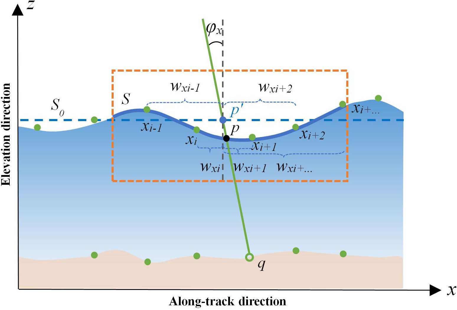
Figure 5. Diagram of the PWCP model used to obtain the local sea-wave profile, S, and the intersection point, p, linked with each seafloor photon.

$\begin{array}{ll}\{\begin{array}{l}z(x)=a_j{x}^3+b_j{x}^2+c_{j}x+d_j\hfill \\ w=\raisebox{1ex}{$1$}\!\left/ \!\raisebox{-1ex}{$\Vert \Vert x-x_{p^{\prime }}\Vert \Vert $}\right.;w=\raisebox{1ex}{$1$}\!\left/ \!\raisebox{-1ex}{${(x-x_{p^{\prime }})}^2$}\right.\hfill \end{array}& (3)\end{array}$

When the sea-wave fluctuation is smooth, the two-order polynomial is suitably utilized in the PWCP model. Correspondingly, the three-order polynomial is utilized. In the two-order polynomial, three parameters of its should be calculated by 3 points. For improving the calculation accuracy with the least square method, four points are needed at least. In the three-order polynomial, five points are needed at least for improving calculation accuracy of its parameters. Generally, one point is added to ensure the stability of calculation accuracy. Assuming that six sea-surface photons are used in the PWCP model, the cubic polynomial parameters for the seafloor photon, q, are solved using the least squares method. Equation 4 represents the error equation, as well as the coefficient matrix A, value matrix L, and unknown vector matrix X as shown in Equation 5:

$\begin{array}{ll}\begin{array}{cc}{v}_i=a_j{x}_i^3+b_j{x}_i^2+c_j{x}_i+d_j-z(x_i)& (i=1,2,\cdots ,6)\end{array}& (4)\end{array}$

$\begin{array}{ll}\begin{array}{cc}A=\left[\begin{array}{cccc}1& x_1& x_1^2& x_1^3\\ 1& x_2& x_2^2& x_2^3\\ ⋮& ⋮& ⋮& ⋮\\ 1& x_6& x_6^2& x_6^3\end{array}\right]& \begin{array}{cc}L=\left[\begin{array}{c}{l}_1\\ l_2\\ ⋮\\ l_6\end{array}\right]& \begin{array}{c}X=\left[\begin{array}{c}{a}_j\\ b_j\\ c_j\\ d_j\end{array}\right]\end{array}\end{array}\end{array}& (5)\end{array}$

Based on the weight equation, weights $w_1$, $w_2$, $\cdots$, and $w_6$ for the six sea-surface photons were calculated, followed by the construction of the weight matrix W. In accordance with the principles of the least squares, the coefficient matrix N for solving the normal equation, accompanied by its corresponding free vector U are created and present as follows. The parameters in the polynomial for the seafloor photon, q, are solved and obtained by matrix X which are represented in Equations 6 and 7, respectively:

$\begin{array}{ll}N=A^{T}WA=\left[\begin{array}{cccc}{w}_1+\cdots +w_6& w_1{x}_1+\cdots +w_6{x}_6& \cdots & w_1{x}_1^3+\cdots +w_6{x}_6^3\\ w_1{x}_1+\cdots +w_6{x}_6& w_1{x}_1^2+\cdots +w_6{x}_6^2& \cdots & w_1{x}_1^4+\cdots +w_6{x}_6^4\\ w_1{x}_1^2+\cdots +w_6{x}_6^2& w_1{x}_1^3+\cdots +w_6{x}_6^3& \cdots & w_1{x}_1^5+\cdots +w_6{x}_6^5\\ w_1{x}_1^3+\cdots +w_6{x}_6^3& w_1{x}_1^4+\cdots +w_6{x}_6^4& \cdots & w_1{x}_1^6+\cdots +w_6{x}_6^6\end{array}\right]& (6)\end{array}$

$\begin{array}{ll}U=\left[\begin{array}{c}{l}_1{w}_1+l_2{w}_2+\cdots +l_6{w}_6\\ l_1{x}_1{w}_1+l_2{x}_2{w}_2+\cdots +l_6{x}_6{w}_6\\ l_1{x}_1^2{w}_1+l_2{x}_2^2{w}_2+\cdots +l_6{x}_6^2{w}_6\\ l_1{x}_1^3{w}_1+l_2{x}_2^3{w}_2+\cdots +l_6{x}_6^3{w}_6\end{array}\right]\hspace{0.33em}\hspace{0.33em}\hspace{0.33em}X=\left[\begin{array}{c}{a}_j\\ b_j\\ c_j\\ d_{}\end{array}\right]=N^{-1}·U& (7)\end{array}$

Subsequently, the local sea-wave profile for the seafloor photon q was determined using the solved polynomial parameters. Finally, the precise calculation of the coordinates of the intersection point p was achieved by utilizing the local sea-wave profile and the constructed spatial line of photon q.

3.2 Refraction correction of seafloor photons

In the x direction, the slope of intersection point p can be determined using the first-order derivative of the cubic polynomial for point p. The first-order derivatives of the polynomial are given by Equation 8, in which symbols $\text{tan}{\theta }_x^p$, ${\theta }_x^p$ and $(x_p,z_p)$ indicate the slope, slope angle, and coordinate of point p, respectively. Normal vector N of point p was calculated using Equation 9:

$\begin{array}{ll}\tan {\theta }_x^p=3a_j{x}_p{}^2+2b_j{x}_p+c_j& (8)\end{array}$

$\begin{array}{ll}N=\frac{-\tan {\theta }_x^p}{\sqrt{1+{\tan }^2{\theta }_x^p}}& (9)\end{array}$

Based on intersection point p, the corresponding slope, $\text{tan}{\theta }_x^p$, seafloor photon, q, and incident angle, φ_x, the different geometric relationships of water refraction were constructed, as illustrated in Figures 6a–c, when $\text{tan}{\theta }_x^p$ is positive, zero, and negative respectively. Within Figure 6, L_x and R_x denote the paths taken by photon q underwater with and without considering water refraction correspondingly. According to Snell’s principle, the relationship between L_x and R_x is formulated as shown in Equation 10:

Figure 6

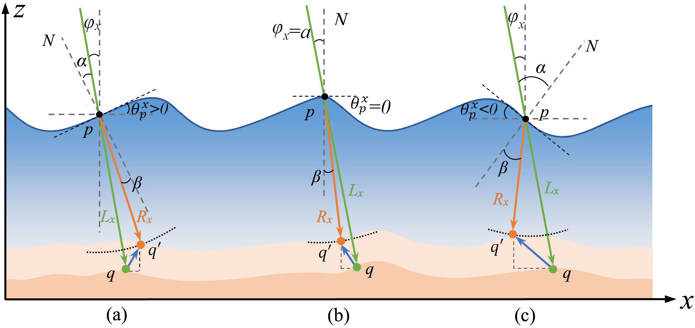
Figure 6. The diagram illustrates the relationship between water refraction and the geometric correlation among the laser pulse, sea wave, and seafloor photon. The black points on the diagram indicate where the laser pulse intersects with the air/sea interface. The green, orange, and blue lines with arrows indicate the original laser path, refracted laser path, and refraction displacement, reflectively. Subfigures a, b, and c represent three different refraction paths under the influence of sea waves.

$\begin{array}{ll}\frac{n_w}{n_a}=\frac{\sin \alpha }{\sin \beta }=\frac{C_a·t/2}{C_w·t/2}=\frac{L}{R}& (10)\end{array}$

where α and β represent the incident and refraction angles, respectively. The symbol n_a denotes the refractive index of air, which is equivalent to 1, while n_w represents the refractive index of water, specifically measured as 1.33 (Xu et al., 2021). Since our study area is located far from continental inputs, the water clarity remains high, and the refractive index closely approximates that of pure water. We selected the refractive index of water as 1.33 based on its well-established value for visible light under standard conditions (approximately 20°C and at a wavelength of 589 nm). This value is widely adopted in optical studies (Hale and Querry, 1973) due to its consistency with experimental measurements of pure water. Additionally, C_a and C_w denote the velocities of laser in air and seawater.

Using the reconstructed local sea-wave profile and geometric relationship of water refraction, the incident angle, α, of a certain seafloor photon can be calculated via the pointing angle,${\phi }_x$, and the slope angle, ${\theta }_x^p$, which is expressed as Equation 11 for the three different angle ranges, such as ${\theta }_x^p\in (0,{\phi }_x)$, ${\theta }_x^p\in ({\phi }_x,{90}^o+{\phi }_x)$, and ${\theta }_x^p\in ({90}^o+{\phi }_x,{180}^o)$. Subsequently, the corresponding refraction angle, β, is acquired with the incident angle, α, and refractive index of air and sea water, represented by Equation 12. Finally, the displacement of seafloor photons caused by water refraction was derived and formulated using Equations 13–16 for the three different cases, where $\Delta x$ and $\Delta z$ represent the displacement in the x and z directions. The symbol $h_q$ denotes the elevation difference between intersection point p where air meet sea and its corresponding photon q located on the seafloor.

$\begin{array}{ll}\{\begin{array}{l}a={\phi }_x-{\theta }_x^p,{\theta }_x^p\in (\mathrm{0,}{\phi }_x)\hfill \\ a={\theta }_x^p-{\phi }_x,{\theta }_x^p\in ({\phi }_x,{90}^o+{\phi }_x)\hfill \\ a=180-{\theta }_x^p+{\phi }_x,{\theta }_x^p\in ({90}^o+{\phi }_x,180)\hfill \end{array}& (11)\end{array}$

$\begin{array}{ll}\beta ={\sin }^{-1}(\frac{n_a}{n_w}·\sin a),(\beta \ge 0)& (12)\end{array}$

$\begin{array}{ll}{L}_x=\frac{h_q}{\cos {\phi }_x}& (13)\end{array}$

$\begin{array}{ll}\{\begin{array}{l}\Delta x=R_x·\sin ({\theta }_x^p+\beta )-L_x·\sin {\phi }_x=L_x·[\sin ({\theta }_x^p+\beta )·\frac{1}{n_w}-\sin {\phi }_x]\hfill \\ \Delta z=L_x·\cos {\phi }_x-R_x·\cos ({\theta }_x^p+\beta )=L_x·[\cos {\phi }_x-\cos ({\theta }_x^p+\beta )·\frac{1}{n_w}]\hfill \end{array},{\theta }_x^p\in (\mathrm{0,}{\phi }_x)& (14)\end{array}$

$\begin{array}{ll}\{\begin{array}{l}\Delta x=R_x·\sin ({\theta }_x^p-\beta )-L_x·\sin {\phi }_x=L_x·[\sin ({\theta }_x^p-\beta )·\frac{1}{n_w}-\sin {\phi }_x]\hfill \\ \Delta z=L_x·\cos {\phi }_x-R_x·\cos ({\theta }_x^p-\beta )=L_x·[\cos {\phi }_x-\cos ({\theta }_x^p-\beta )·\frac{1}{n_w}]\hfill \end{array},{\theta }_x^p\in ({\phi }_x,{90}^o+{\phi }_x)& (15)\end{array}$

$\begin{array}{ll}\{\begin{array}{l}\Delta x=R_x·\sin ({\theta }_x^p+\beta -{180}^o)-L_x·\sin {\phi }_x=-L_x·[\sin ({\theta }_x^p+\beta )·\frac{1}{n_w}+\sin {\phi }_x]\hfill \\ \Delta z=L_x·\cos {\phi }_x-R_x·\cos (180-{\theta }_x^p-\beta )=L_x·[\cos {\phi }_x+\cos ({\theta }_x^p+\beta )·\frac{1}{n_w}]\hfill \end{array},{\theta }_x^p\in ({90}^o+{\phi }_x,{180}^o)& (16)\end{array}$

In terms of the y direction, it is not possible to reconstruct the sea wave profile due to the linear scanning mechanism employed by ATLAS, as illustrated in Figure 3. However, displacements of each seafloor photon in this direction are influenced by the fluctuating sea surface. This variation arises due to the varying elevation and underwater path distance of each seafloor photon’s corresponding intersection point with the sea surface, as shown in Figure 6. The projection of these air-sea intersection points forms a vertical line along the y-axis, as shown in Figure 7a by a black vertical dashed line within the gray plane. Here, p, p₁, and p₂ represent different sea surface intersection points corresponding to different seafloor photons. Figure 7b illustrates that different intersection points have different heights in the elevation direction, resulting in a variety of laser pulse paths in the water body.

Figure 7

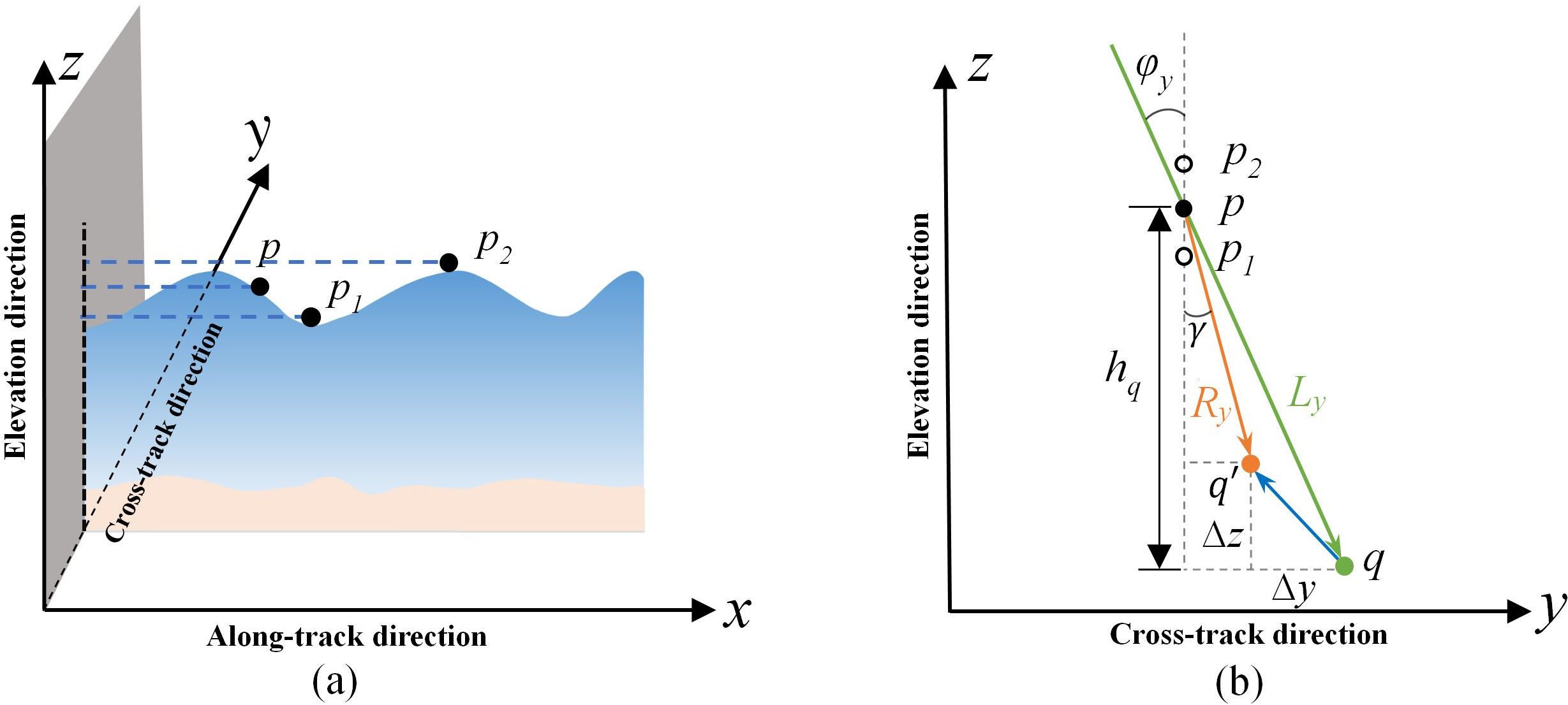
Figure 7. Displacements of each seafloor photon in the y direction. (a) Geometric projection of where the laser pulse intersects with sea surface. (b) Various intersection points in the y direction and their corresponding geometric relationships before and after water refraction.

Considering the geometric relationship before and after water refraction in the y direction, the refraction displacement, $\Delta y$, of photon q is derived and expressed as Equation 17, in which the refraction angle, $\gamma$, and the original underwater laser path, $L_y$, can be calculated from Equations 18 and 19. The along-track elevation difference, $h_q$, represents the vertical separation between point p where the air and sea intersect, and its corresponding photon q located on the seafloor.

$\begin{array}{ll}\Delta \text{y}=L_y·\sin {\phi }_y-R_y·\sin ({\phi }_y-\gamma )=L_y·[\sin {\phi }_y-\sin ({\phi }_y-\gamma )·\frac{1}{n_w}]& (17)\end{array}$

$\begin{array}{ll}{L}_y=\frac{\cos {\phi }_x·L_x}{\cos {\phi }_y}=\frac{h_q}{\cos {\phi }_y}& (18)\end{array}$

$\begin{array}{ll}\gamma ={\sin }^{-1}(\frac{n_a}{n_w}·\sin {\phi }_y)& (19)\end{array}$

3.3 Coordinate correction of seafloor photon

To perform the adjustment of coordinate in WGS-84 geographical system (consisting of latitude, longitude, and elevation), the refractive displacement of each photon on the seafloor should be projected onto the WGS-84 ellipsoid. Figure 8 illustrates the geometric projection correlation among latitude, longitude and spatial distance within the WGS-84 ellipsoid, in which the green and orange points, $q$ and $q^{\prime }$, respectively, represent the original photon and the photon after coordinate correction. In Figures 8a, b, the blue curve represents the coordinate displacement of the original photon in terms of longitude and latitude. Lines N and M are the normal line of the longitudinal line and the flattening radius of the meridian, respectively.

Figure 8

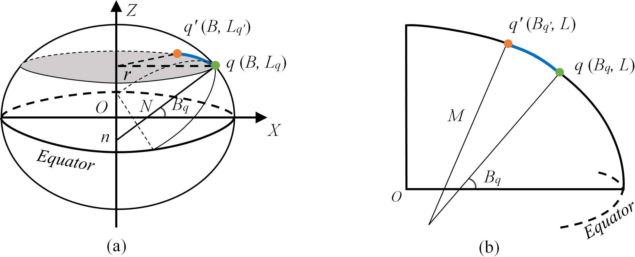
Figure 8. The relationship between the refraction displacement of seabed photons in both (a) longitudinal and (b) latitudinal directions and their geometric projection onto the WGS-84 ellipsoid.

By utilizing the geometric projection correlation, the coordinates of the seafloor photon in ATL03 ($B_q^0$, $L_q^0$, $H_q^0$) were corrected and expressed as ($B_q$, $L_q$, $H_q$) using Equations 20 and 21, respectively. Symbols $A^{\prime }$, $B^{\prime }$,’ $C^{\prime }$, $D^{\prime }$, $E^{\prime }$,’ $V_0^{\text{'}}$, and $W_0^{\text{'}}$ are the calculation parameters that do not have a concrete meaning. The semi-major axis of the ellipse in the equatorial plane is denoted by a. Based on the refraction displacement in different directions, the length of the refraction displacement projected on the parallel and meridian circles is represented by $S_L$ and $S_B$, formulated in Equation 22:

$\begin{array}{ll}\{\begin{array}{l}{B}_q=\frac{{V^{\prime }}_0+{W^{\prime }}_0}{a(1-e^2)A^{\prime }}\hfill \\ L_q=L_q^0+\frac{S_L}{N\cos B_q^0}\hfill \\ H_q=H_q^0+\Delta \text{z}\hfill \end{array}& (20)\end{array}$

$\begin{array}{ll}\{\begin{array}{l}{V^{\prime }}_0=S_B+a(1-e^2)(A^{\prime }·arc{B}_q^0-B^{\prime }·\sin 2B_q^0+C^{\prime }·\sin 4B_q^0-D^{\prime }·\sin 6B_q^0+E^{\prime }·\sin 8B_q^0)\hfill \\ {W^{\prime }}_0=a(1-e^2)(B^{\prime }·\sin 2B_q-C^{\prime }·\sin 4B_q+D^{\prime }·\sin 6B_q-E^{\prime }·\sin 8B_q)\hfill \end{array}& (21)\end{array}$

$\begin{array}{ll}\{\begin{array}{c}{S}_L=\Delta \text{x}\cos \phi -\Delta y\sin \phi \\ S_B=\Delta \text{x}\sin \phi +\Delta y\cos \phi \end{array}& (22)\end{array}$

4 Experimental results

4.1 Sea-wave profile fitting and photon ray tracing

Eight ATL03 ground tracks were used in this research, employing a high-accuracy adaptive variable ellipse filtering bathymetric method (AVEBM) to obtain the signals photon from the sea surface and the seafloor (Chen et al., 2021a). To automatically separate and detect the effective photon of the water surface and bottom, an ellipse filter is adopted in the AVEBM, with the filter size changing with different water depths and the density distributions of the water-column photon. To realize this aim, the proposed method has five parts, namely a) vertical segments and Gaussian curve fitting, b) separation of the above-water, water surface, and water-column photons, c) determining initial parameters of the elliptical filter, d) establishing the relationship between the initial ellipse filter and the water-column photon density, and e) detecting and fitting the different types of detected effective photons.

To assess the fitting precision and consistency of the sea-wave profile, the photon signal located at the sea surface was obtained by local fitting of the PWCP with different intervals. Figure 9a illustrates the sea-wave profile fitting and photon ray tracing, in which the sea surface and seafloor photons are denoted by blue and orange points. Points $p^{\prime }$ and $p$ denote the intersection points of the reconstructed transmission path of seafloor photon q with mean sea surface $S_0$ and the local sea-wave profile. Using different interval widths, Figure 9 (b) displays the various fitting outcomes of the PWCP for a certain seafloor photon selected in 20181021GT1L, where the blue point represents the sea surface photon, as well as the red, green, and violet curves illustrate the fitting results at intervals of 6, 8, and 10 m, respectively. Figure 9c shows the root mean squared error (RMSE) of the fitting results at different intervals ranging from 4 to 15 m.

Figure 9

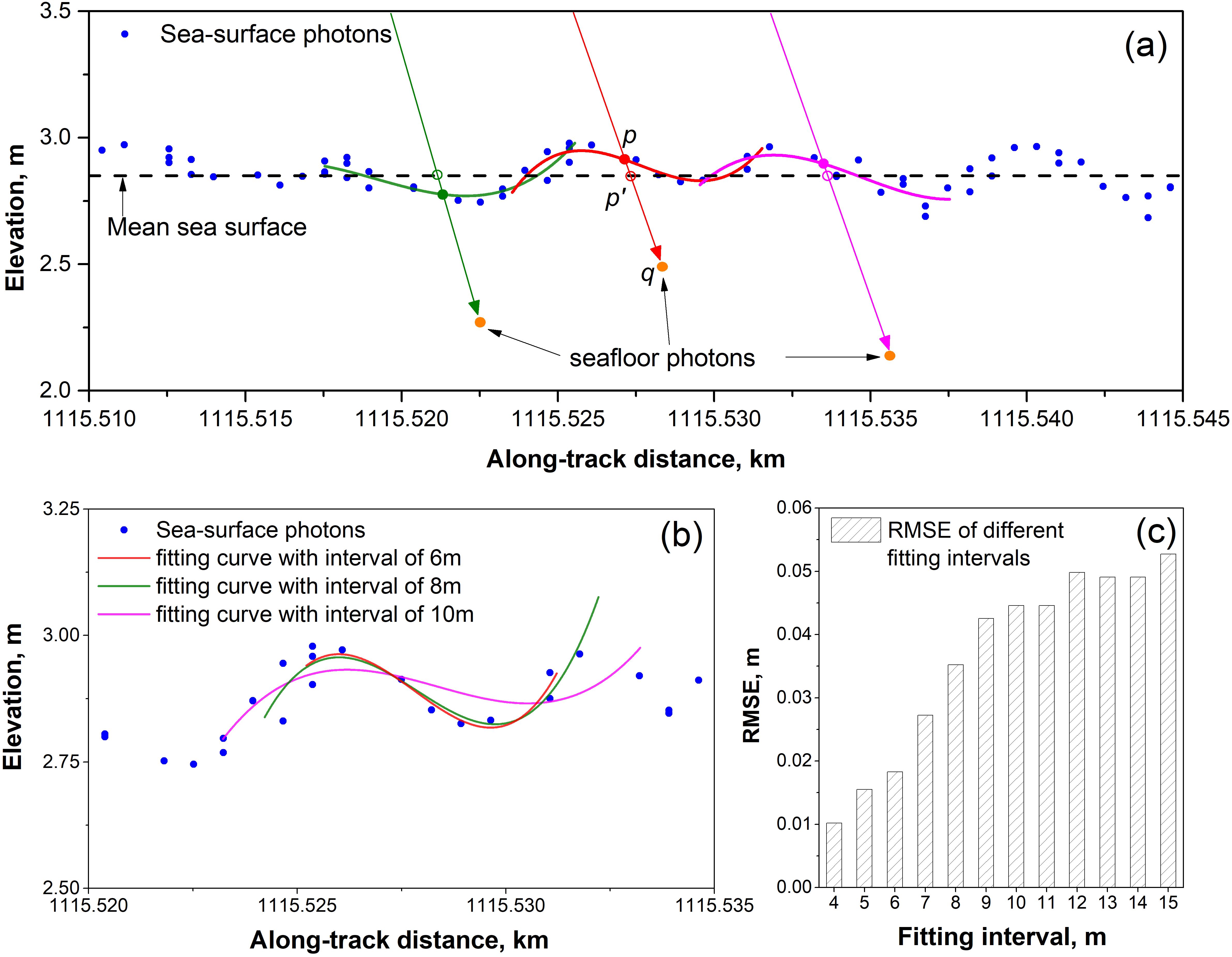
Figure 9. (a) Schematic diagram of sea-wave profile fitting using PWCP, (b) statistically calculated fitting intervals, and (c) fitting accuracy variations for the 20181021GT1L dataset.

The statistical results show that a shorter fitting interval has a higher fitting accuracy for the sea-wave profile. For ICESat-2, the sample interval of the photon was 0.7 m. However, the short fitting interval generally covered the smaller number of sea-surface photons; the sea-surface photon may be missing in some sample intervals owing to various factors. According to the statistical analysis of the number and distribution of sea-surface photons in the eight ATL03 datasets obtained in the study areas, the number of the sea-surface photons was set as 6 to adoptively determine the fitting interval in the PWCP. Table 2 presents the mean height of sea-wave and the RMSE obtained from fitting the sea-wave profile for each track dataset as well as all datasets, using a fitting interval of 5 m. The RMSE of each dataset ranged from 0.015 to 0.023 m; the average RMSE of all datasets reached 0.019 m.

Table 2

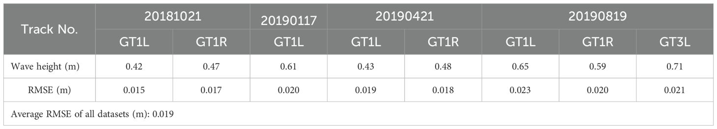
Table 2. The mean wave height and RMSE from fitting the sea-wave profile for each dataset and all datasets based on the PWCP model with a fitting interval of 5 m.

4.2 Results of refraction correction and coordinate compensation

The refraction correction was done by utilizing the reconstructed sea-wave profile and the point where the laser pulse path intersects with the air/sea interface. Figures 10c, d display the correction results for 20181021GT1L and 20181021GT1R, which represent a pair of ground tracks. These tracks are denoted by the corresponding red-dashed and solid lines depicted in Figure 10a. The correction result for 20190819GT1L, which had a high-density photon distribution, is shown in Figure 10e. This ground track is shown by the yellow line in Figure 10b.

Figure 10

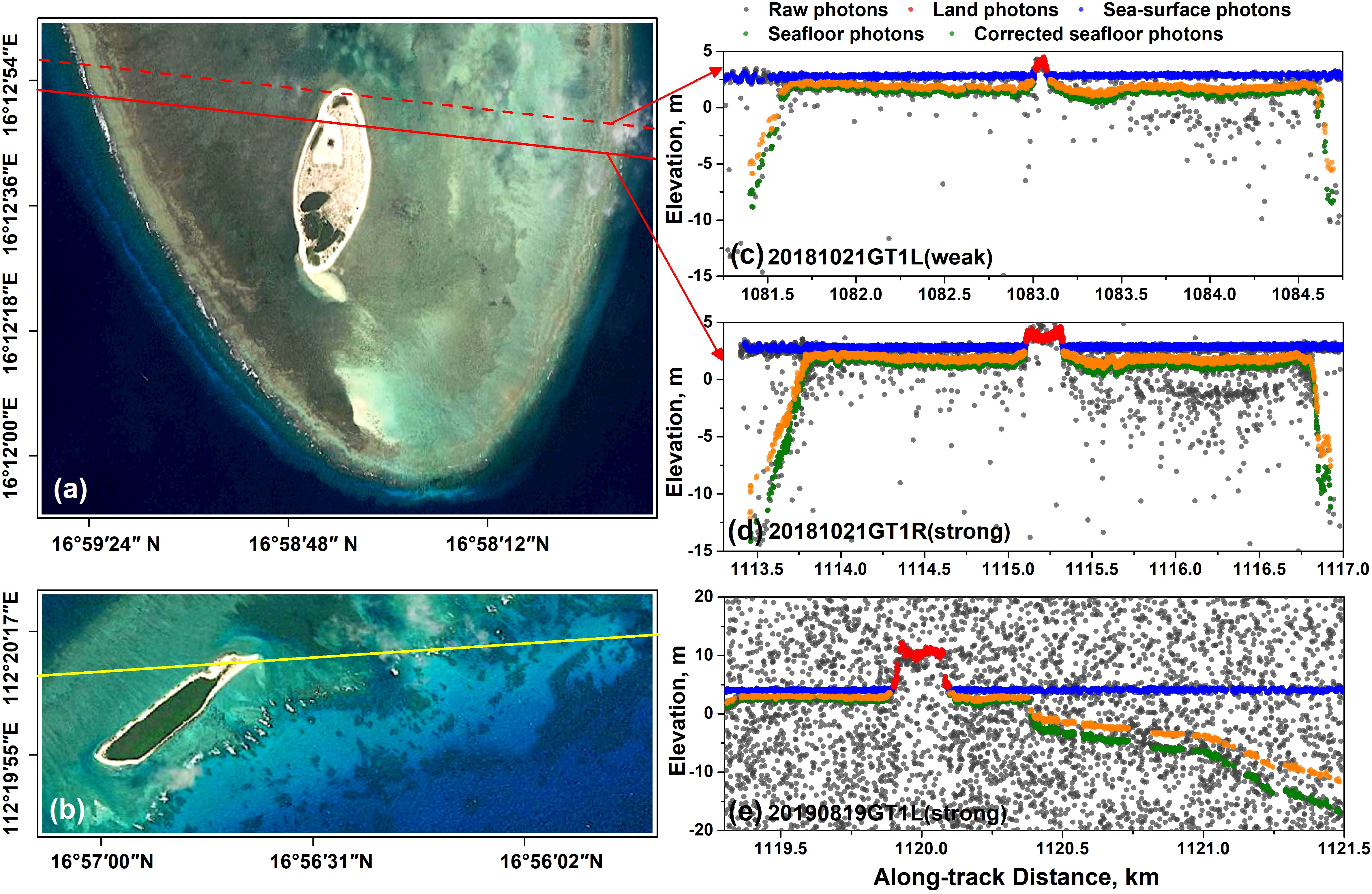
Figure 10. Ground tracks of 20181021GT1L and 20181021GT1R shown in (a) and the corresponding correction results illustrated in (c, d), respectively. Ground track and refraction correction result of 20190819GT1L, which has a high-density photon distribution, shown in (b, e).

Additionally, Table 3 outlines the range of water depths before and after refraction correction, along with the range of displacements in the elevation direction for the eight tracks. In this table, various bathymetric results were obtained with tide correction to ensure and enhance the precision and reliability of bathymetric result. Before the refraction correction, the recorded water depths ranged from -0.15 m for 20190117GT1L and -21.47 m for 20190819GT1L. Correspondingly, the minimum and maximum water depths were measured as -0.12 m for 20190117GT1L and -16.01 m for 20190819GT1L after refraction correction. The respective elevation displacement caused by refraction amounted to 0.03 and 5.46 m.

Table 3

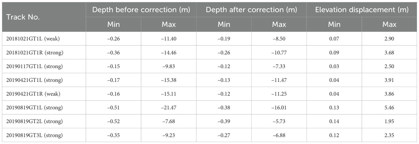
Table 3. Comparisons of the minimum and maximum bathymetry result before and after refraction correction, along with the corresponding elevation displacement observed in the eight-track datasets of ATLAS acquired at the study areas.

The displacements caused by refraction in different directions were statistically computed and denoted as $\Delta x$ and $\Delta y$. Moreover, using the coordinate correction method, the displacements of each seafloor photon in different directions were projected to the latitude and longitude of the WGS-84 ellipsoid, denoted as ΔB and ΔL. This ensures and enhances the accuracy of seafloor photons and the precision of underwater topography. Table 4 presents the range of displacements observed in the eight ground tracks, encompassing both x and y directions, along with the corresponding latitude and longitude displacements. Negative values in this table indicate that the displacement direction is opposite to the x or y directions, which is caused by the different geometric refraction relationships.

Table 4

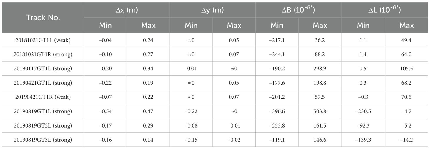
Table 4. The displacements in both the x and y directions, along with the corresponding latitude and longitude coordinate displacement for the eight-track datasets of ATLAS located at the study areas.

The displacement in $\Delta x$, $\Delta y$, ΔB and ΔL (Table 4) was small relative to the displacement of $\Delta z$. In the x direction, ground tracks 20190819GT1L and 20181021GT1L exhibited the widest range between maximum and minimum displacement, with values ranging from -0.54 to 0.47 m and from -0.04 to 0.24 m, respectively. The relative displacements in these tracks reached a maximum of 1.01 m and a minimum of 0.28 m. In the y direction, the displacement was very small and the maximum displacement ranged from -0.22 m to zero for 20190819GT1L. Correspondingly, the displacement values for latitude and longitude were extremely small, at the level of 10–⁸ degree. The highest displacements for latitude and longitude occurred for track 20190819GT1L, ranging from -396.6 to 503.8 10–⁸ deg and from -230.5 to -4.7 10–⁸ deg. For 20181021GT1L, there was a minimum displacement in latitude and longitude, ranging from -217.1 to 36.2 10–⁸ deg and from 1.1 to 49.4 10–⁸ deg.

In Table 4, the x-direction displacement is more pronounced than in the y direction. This difference arises because our method can determine varying slopes and incident angles in the x direction using the laser beam’s pointing angle and the reconstructed sea wave. In contrast, while the slope at the air/sea intersection in the y direction cannot be directly determined, the fluctuating height of this point can be measured. The refraction displacement in the y direction is thus calculated based on the laser beam’s pointing angle and the photon’s transmission path. The smaller pointing angle in the y direction results in less displacement compared to the x direction.

4.3 Bathymetric accuracy and validation

The bathymetric results of the tracks were corrected using the tide data recorded by the tide station to eliminate the error caused by tidal influence and perform a comparison with the in-situ data (Guan et al., 2019). Figure 11 presents a comparison between the bathymetric results of all the tracks after refraction correction and the in-situ bathymetry, in which various colored circles, triangles, and squares indicate the different scatter point distribution relationships of the bathymetry of the different track datasets with the in-situ data.

Figure 11

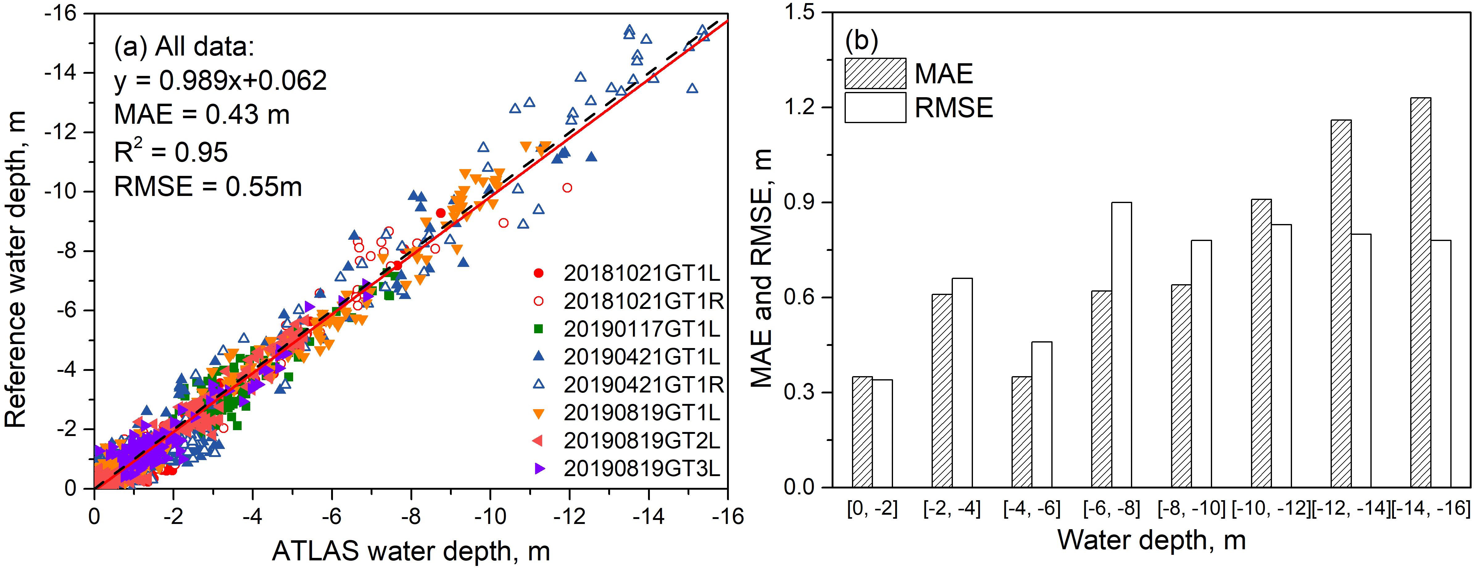
Figure 11. (a) Distribution of the scatter point and assessment of the (b) bathymetric accuracy between bathymetry result after refraction correction and in-situ data for all eight-track datasets.

The determination coefficient (R²), mean absolute error (MAE), and RMSE were statistically calculated, as presented in Figure 11a. For all the tracks, the value of R², MAE, and RMSE reached 0.955, 0.43 m, and 0.55 m. Figure 11b presents the MAE and RMSE values at the different water depths, in which the minimum MAE value was approximately 0.3 m and appeared at a depth range from 0 to -2 m and from -4 to -6 m, respectively. The corresponding maximum value was approximately 1.2 m located between -14 and -16 m. Additionally, the minimum RMSE value was approximately 0.3 m when the water depth ranged from 0 and -2 m; the corresponding maximum was located between -6 and -8 m, reaching 0.9 m.

Table 5 lists the R², MAE, and RMSE of each track before and after refraction correction to analyze the influence of refraction on bathymetry in detail. Before the refraction correction, the MAE values ranged from 2.91 m for 20190819GT1L to 0.26 m for 20190421GT1L. After the refraction correction, these MAE values decreased to 0.61 and 0.41 m. The R² value of each dataset remained unchanged before and after the refraction correction. In addition, the change in RMSE value was relatively smaller compared to that of the MAE value. RMSE values for 20190819GT3L and 20190421GT1L were reduced from a minimum of 0.52 m to 0.40 m and from a maximum of 1.13 m to 0.81 m, respectively. The highest accuracy for the bathymetry, after the refraction correction, reached 0.26 m for the MAE and 0.38 m for the RMSE in 20190819GT2L.

Table 5

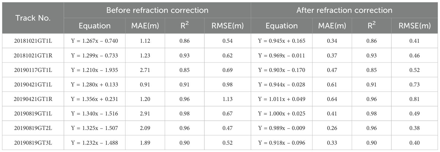
Table 5. Comparison of bathymetric accuracy before and after implementing refraction correction for eight-track ATLAS datasets.

5 Analysis and discussion

5.1 Analysis of sea-wave profile fitting with PWCP

As illustrated in Figures 8b, c, opting for a shorter fitting interval in the PWCP yielded superior accuracy in fitting the sea-wave profile. Figure 8c shows that the highest fitting accuracy was approximately 0.01 m of the RMSE when using the fitting interval of 4 m. However, during the process of sea-wave profile fitting, the sea-surface photons may be missing in some sample intervals of ATLAS, e.g., 0.7 m, which would result in an insufficient number of sea-surface photons in the polynomial parameter solutions and yielding decrements of the fitting accuracy. For this situation, six water-surface photons located at both the left and right sides of the intersection point was used to calculate the curve parameters of PWCP and reconstruct the corresponding instantaneous curve of the sea waves. The number of the water surface photons is utilized to determine the fitting interval, which actually is an adoptive selection of the fitting interval. Therefore, this method can be used to other track datasets obtained at all areas. In our experiments, when a certain seafloor photon required refraction correction, we selected and used six water surface photons to reconstruct the corresponding instantaneous curve of the sea waves (Chen et al., 2021a; Zhang et al., 2022).

Additionally, for the eight ground tracks, the average wave height was statistically calculated (Table 2), which ranged from 0.42 to 0.71 m. Considering these factors, the fitting interval for the PWCP was generally 5 m to ensure the high-accuracy reconstruction of the sea-wave profile and to precisely determine the intersection point for each photon on the seafloor. Finally, the results listed in Table 2 reveal that the fitting accuracy of the sea-wave profile achieved an exceptionally high level, reaching accuracy down to the centimeter.

5.2 Analysis of refraction influence and bathymetric accuracy

Figures 9c, d illustrates that the seafloor photon number detected by the strong laser pulse was notably greater than that by the weak laser pulse, which became more significant with the increasing water depth. According to Table 3, the maximum water depth detected by two adjacent weak and strong laser beams (20181021GT1L and 20181021GT1R) was -8.50 and -10.77 m, and their difference reached 2.27 m. For 20190421GT1R and 20190421GT1L, a difference of 0.22 m was observed in the maximum water depth. For the above two pairs of laser beams, the difference in the maximum water depth, i.e., 2.27 and 0.22 m, had a relatively large difference, mainly caused by the different environment between the water body and atmosphere in the two data acquisition periods. However, for each pair of laser beams, the environment of the water body and atmosphere should be the same because the ground scanning interval in the pair of weak and strong laser beams is close to 90 m (Parrish et al., 2019). This indicates that the environmental conditions of the water body and atmosphere at the time of acquiring datasets 20190421GT1R and 20190421GT1L were better than those of 20181021GT1L and 20181021GT1R. Both the weak and strong laser beams could penetrate the sea surface to almost the same water depth.

Based on Tables 3 and 4, there is a positive correlation between water depth and the refractive displacement. Additionally, the displacement in the z direction surpassed that in both the x and y directions, which was determined by the complex geometric relationship between the wave height, laser pulse pointing angle, and water depth. Compared to the displacement observed in the y direction, the displacement along the track was relatively large owing to the instantaneous sea-wave profile. Most displacements in the y direction, as documented in Table 4, approached zero. Therefore, when evaluating the bathymetric results of ICESat-2, it is possible to neglect the potential influence of displacement in this direction (Coveney et al., 2021).

Findings presented in Table 5 demonstrated that refraction correction plays a pivotal role in nearshore bathymetry when utilizing the ATLAS dataset. After refraction correction, the bathymetric accuracy of the MAE improved significantly. Compared to the MAE, the RMSE value improved relatively less. Analyzing the experimental data and results, a large number of the detected seafloor photons were situated within the depth range of 0 to -6m, as demonstrated in Figure 10a. In this depth range, the displacement is relatively small. In contrast, a large displacement mainly occurs at a deeper range; the number of seafloor photons in this range is relatively small, which results in a smaller improvement in the RMSE. According to the comparisons of the in-situ data with the bathymetric results of all eight-track datasets and each track dataset before and after water refraction, the different bathymetric results were validated and had high-accuracy.

Furthermore, the remote sensing retrieval technique was employed to obtain the nearshore bathymetry of the entire study area. This involved utilizing the multi-spectrum image captured by Sentinel-2 satellite and incorporating the bathymetric data from ATLAS (Xu et al., 2021; Liu et al., 2024). The Sentinel-2 satellite Level-2A image acquired on 13 October 2021 was downloaded from the Copernicus data center (https://scihub.copernicus.eu/dhus/#/home) of the European Space Agency (Drusch et al., 2012; Toming et al., 2016). The blue and green band with resolution of 10m from the Sentinel-2 image, as well as the ICESat-2 bathymetric points, were used to build the SDB model (Yang et al., 2022). In this research, the widely used band ration model proposed by Stumpf et al. were utilized to produce the bathymetric maps. This model used a ratio logarithmic transformation to capture the relationship between the reflectance of image and the ICESat-2 water depth, and the bathymetric maps which was shown in Figure 12a.

Figure 12

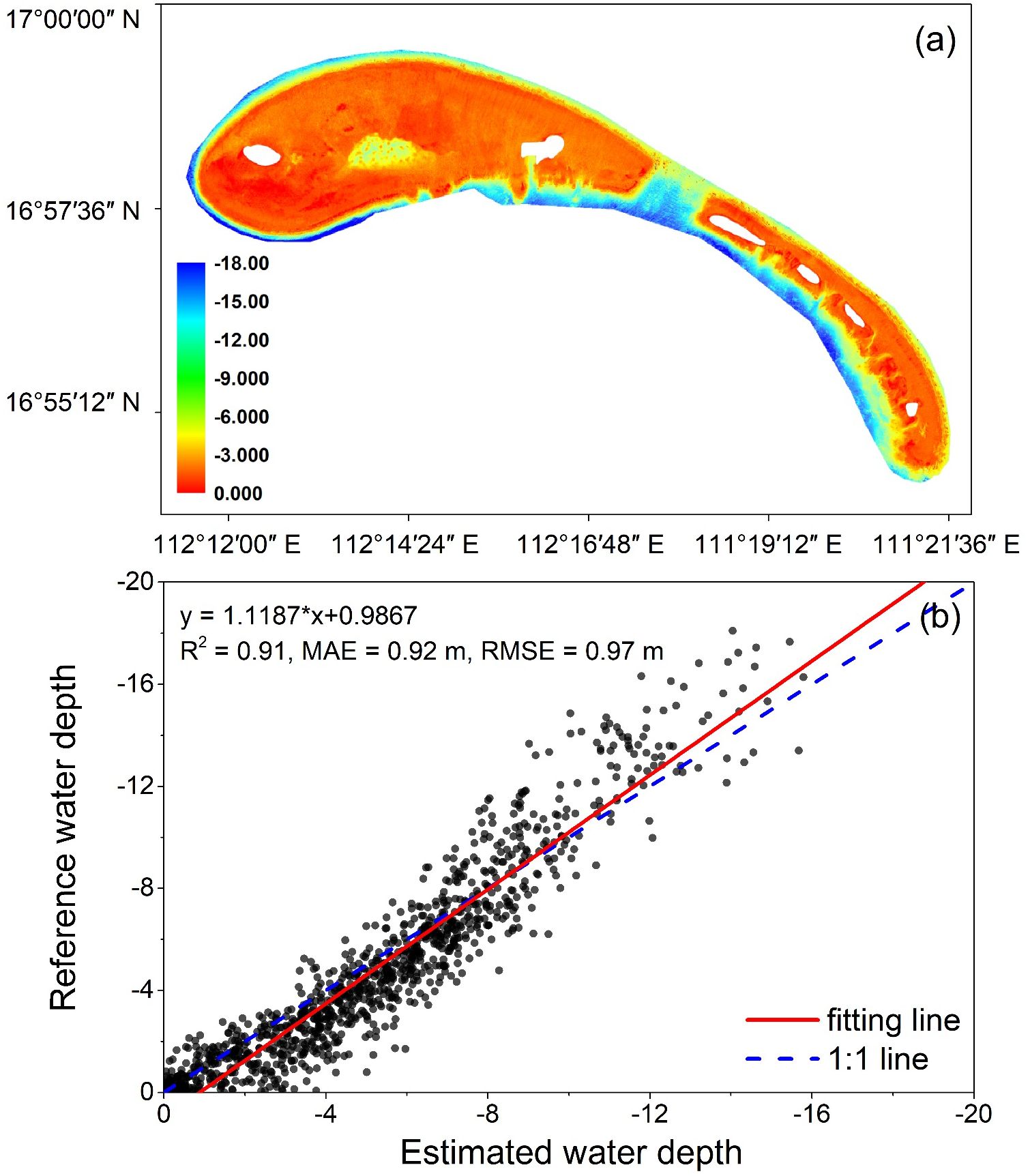
Figure 12. (a) Bathymetric results based on Sentinel-2 multispectral imagery and (b) their comparison with ATLAS bathymetric results.

In comparison with the in-situ data, the bathymetric accuracy was assessed through the metrics of R², MAE, and RMSE, yielding corresponding values of 0.91, 0.92 m, and 0.97 m, respectively (Figure 12b). In summary, based on various validations of the bathymetric results, the PWCP model advocated for ICESat-2 exhibits exceptional levels of accuracy, reliability, and precision when employed in the mapping of nearshore bathymetry and underwater topography.

5.3 Comparing water refraction correction with different methods

Comparing experiments between methods proposed in this manuscript and the previous published paper that the sea surface was assumed as the plane, it is demonstrated that the fluctuation sea wave would has the relatively big impact on the result accuracy of the water refraction and the nearshore bathymetry. As shown in Figures 13a–c, the same track dataset of ATL03 (20181021GT1R) has been used to achieve the signal photon extraction located on the sea surface and bottom. Subsequently, the water refraction correction has been performed by the proposed method based on sea-wave profiles with a piece-point polynomial and the previous method that sea surface was simplified as the plane, which is represented by Figure 13a. As shown in Figures 13b, c, the maximum results deviation of the water refraction correction reached around 0.5 m, where the sea wave has the bigger fluctuation represented by the local amplification area in Figure 13a. Counting the bathymetric results obtained by the different refraction correction methods, the deviation of the bathymetric accuracy reaches around 0.1 m RMSE, which is determined by the fluctuation degree of the sea wave. This deviation approximately accounts for one fifth of the bathymetric accuracy with ICESat-2.

Figure 13

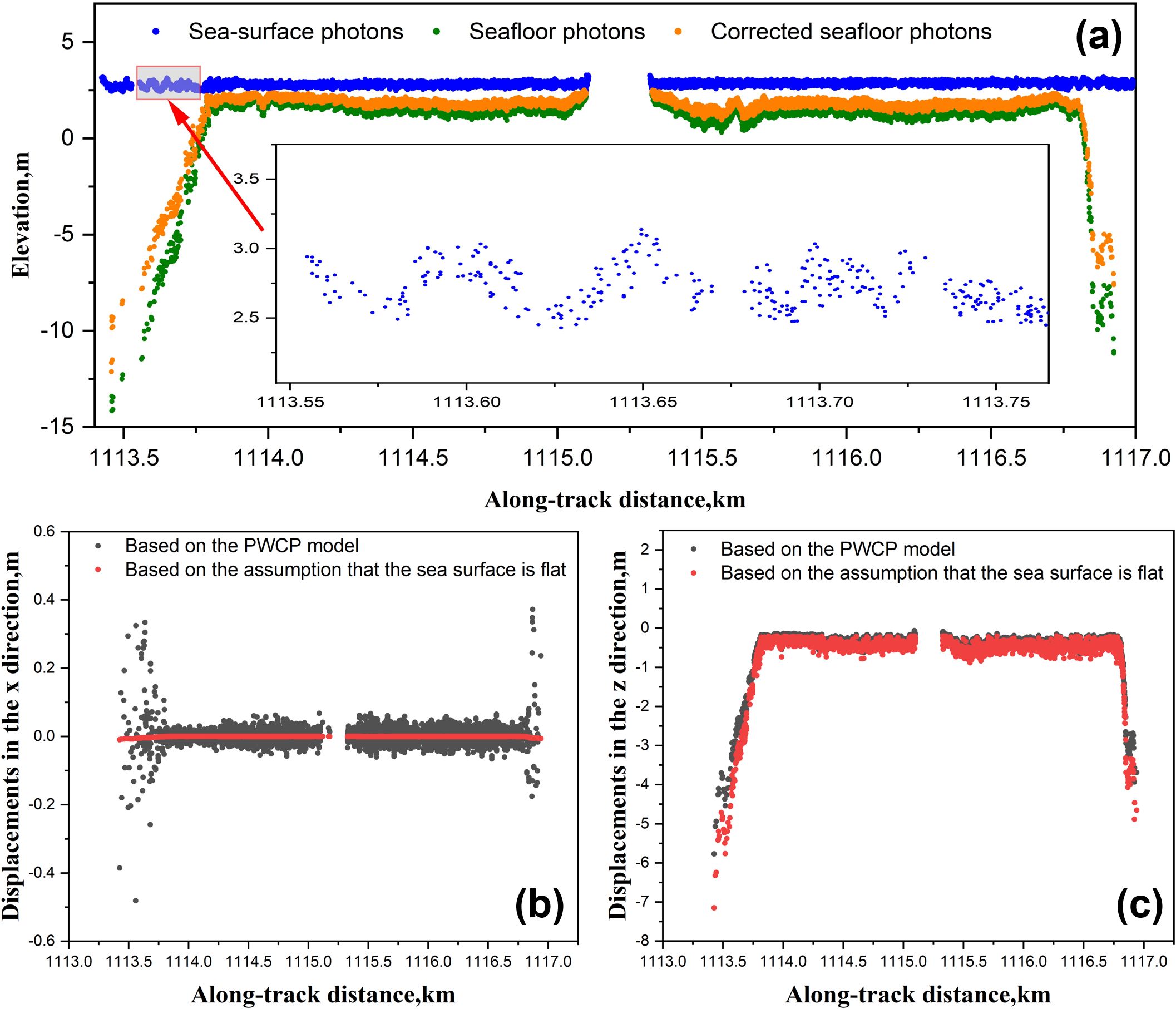
Figure 13. Comparing the water refraction correction with the method based on sea-wave profiles with a piece-point polynomial and the method that sea surface was simplified as the plane. The dataset of 20181021GT1R was used to extract the signal photons of sea surface and floor shown in (a). The deviation of the refraction correction and bathymetric result with different methods were represented by (b, c).

5.4 Relationship for refraction influence with different factors

Refraction correction in nearshore bathymetry using ATLAS datasets involves a complex geometric relationship influenced by factors such as wave height, laser pulse pointing angle, and water depth (Ma et al., 2020; Zhang et al., 2022). To scrutinize and investigate the relationship between refraction and wave height, incident angle, and water depth, simulations were conducted to ascertain the displacements in different directions caused by various wave heights and pointing angles across varying water depths. These simulations are depicted by the array of colored lines showcased in Figure 14. Wave heights of 1, 3, and 5 m, and the various of laser pulse pointing angle, ranging from 5 to 25° at intervals of 5°, were simulated and utilized to reveal the variety of displacements in $\Delta x$, $\Delta y$, and $\Delta z$ in the different water depths and to analyze their relationship in detail.

Figure 14

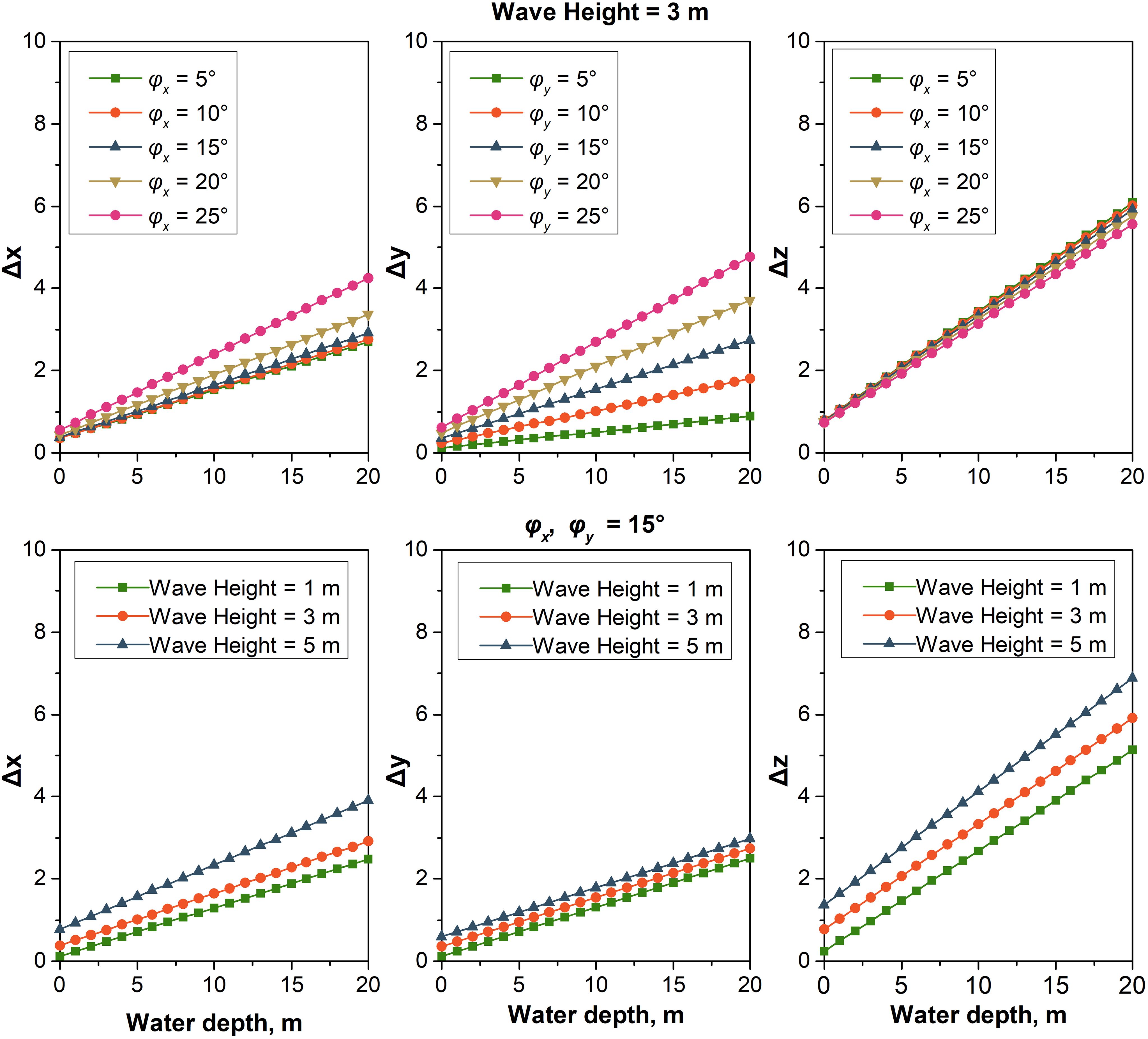
Figure 14. Relationship for refraction displacement in different directions caused by the various wave heights, laser pulse pointing angles, and water depths, represented by the various colored lines.

As shown in Figure 14, when the wave height was 3 m, the displacements of $\Delta x$, $\Delta y$, and $\Delta z$ were enhanced with the increased pointing angles of ${\phi }_x$ and ${\phi }_y$. The displacement of $\Delta y$ had the largest change rate compared to that of $\Delta x$ and $\Delta z$, with an increasing pointing angle. The variations in $\Delta x$ and $\Delta z$ were relatively minor, with $\Delta z$ experiencing the smallest rate of change. This phenomenon occurred because the refraction correction factored in the sea-wave profile, and the various incident angles were obtained by the different normal vectors, N, at intersection points on the sea surface (Figure 5). When the laser pulse pointing angle was 15° (Figure 14), the higher wave height would increase the displacements of $\Delta x$, $\Delta y$, and $\Delta z$ in the different water depths. Additionally, the change rate of $\Delta y$ was at a minimum because the plane refraction correction was performed at a different height (Figure 6). The change rate of $\Delta x$ was relatively large and the change rate of $\Delta z$ was at a maximum, which illustrates that different wave heights had notable impacts on the displacements of $\Delta x$ and $\Delta z$ during refraction correction. In summary, by simulating and analyzing of the relationship between refractive displacements and different wave heights, incident angles, and water depths, we have substantiated the correctness of the proposed method, which leverages the reconstruction of the sea-wave profile.

6 Conclusions

This research introduces a new approach, named PWCP, for addressing refraction correction, which relies on the ray tracing of each seafloor photon and sea-wave profile reconstruction. Using the extracted signal photon of water surface, the instantaneous sea wave has been modeled with PWCP. The rigorous space geometry relation of laser pulse penetrating the air-water interface of sea wave to the seafloor was established. For each seafloor signal photon, the air/sea intersection points can be calculated, and the corresponding slope, incident and refraction angles can be determined. Through the rigorous space geometry relation established, the novel refraction correction method is proposed and unitized to improve the absolute and relative positions accuracy of the seafloor signal photon. Meanwhile, the accuracy of the nearshore bathymetry could also be increased relative to the previous study, in which the water surface was assumed as the plane. Additionally, a coordinate correction model was proposed to correct and obtain high-accuracy coordinates of the seafloor photons. According to the results of these experimental and statistical analysis, it is evident that the PWCP model efficiently enhances the precision of nearshore bathymetry. The maximum corrected depth displacement in the study area was 5.46 m at a water depth of 16.01 m. In the along-track direction, the displacement ranged from -0.54 to 0.47 m and the maximum relative displacement reached 1.01 m, which was notably larger than the displacement observed in the cross-track direction, primarily owing to the small pointing angle in this direction. Finally, displacements with various wave heights and pointing angles were simulated and used to analyze the relationship between wave height, incident angle, water depth and the influence of refraction, which further demonstrated the accuracy and reliability of the proposed PWCP model for ICESat-2. Comparing to the previous studies, the novel can effectively ensure the absolute and relative positions accuracy of the seafloor signal photon further for improving the nearshore bathymetrical and underwater topographical accuracy. Future research should be conducted using ATLAS datasets and remote-sensing images with different resolutions to delve into the capabilities of ICESat-2 for nearshore bathymetry across diverse water environments.

Data availability statement

The original contributions presented in the study are included in the article/supplementary material. Further inquiries can be directed to the corresponding author.

Author contributions

YC: Conceptualization, Methodology, Validation, Writing – original draft, Writing – review & editing. QZ: Data curation, Investigation, Writing – original draft, Writing – review & editing. YL: Funding acquisition, Project administration, Supervision, Writing – original draft, Writing – review & editing. LW: Investigation, Writing – review & editing. WS: Data curation, Writing – review & editing. LZ: Validation, Writing – review & editing. LZW: Investigation, Writing – review & editing.

Funding

The author(s) declare that financial support was received for the research and/or publication of this article. This work was supported by the National Key Research and Development Program of China (Grant No. 2023YFB3907705-3), the National Natural Science Foundation of China (Grant No. 42171373), the Key Laboratory of Geological Survey and Evaluation of Ministry of Education (Grant No. GLAB2023ZR09), the Special Fund of Hubei Luojia Laboratory (Grant No. 220100035), and the Open Research Program of the International Research Center of Big Data for Sustainable Development Goals (Grant No. CBAS2023ORP03).

Conflict of interest

The authors declare that the research was conducted in the absence of any commercial or financial relationships that could be constructed as a potential conflict of interest.

Generative AI statement

The author(s) declare that no Generative AI was used in the creation of this manuscript.

Publisher’s note

All claims expressed in this article are solely those of the authors and do not necessarily represent those of their affiliated organizations, or those of the publisher, the editors and the reviewers. Any product that may be evaluated in this article, or claim that may be made by its manufacturer, is not guaranteed or endorsed by the publisher.

References

Albright A., Glennie C. (2020). Nearshore bathymetry from fusion of Sentinel-2 and ICESat-2 observations. IEEE Geosci. Remote Sens. Lett. 18, 900–904. doi: 10.1109/LGRS.2020.2987778

Crossref Full Text | Google Scholar

Bernardis M., Nardini R., Apicella L., Demarte M., Guideri M., Federici B., et al. (2023). Use of ICEsat-2 and sentinel-2 open data for the derivation of bathymetry in shallow waters: case studies in sardinia and in the venice lagoon. Remote Sens. 15, 2944. doi: 10.3390/rs15112944

Crossref Full Text | Google Scholar

Cao B., Wang J., Hu Y., Lv Y., Yang X., Gong H., et al. (2023). ICESAT-2 shallow bathymetric mapping based on a size and direction adaptive filtering algorithm. IEEE J. Selected Topics Appl. Earth Observations Remote Sens. 16, 6279–6295. doi: 10.1109/JSTARS.2023.3290672

Crossref Full Text | Google Scholar

Chen Y., Le Y., Zhang D., Wang Y., Qiu Z., Wang L. (2021a). A photon-counting LiDAR bathymetric method based on adaptive variable ellipse filtering. Remote Sens. Environ. 256, 112326. doi: 10.1016/j.rse.2021.112326

Crossref Full Text | Google Scholar

Chen Y., Zhu Z., Le Y., Qiu Z., Chen G., Wang L. (2021b). Refraction correction and coordinate displacement compensation in nearshore bathymetry using ICESat-2 lidar data and remote-sensing images. Optics Express 29, 2411–2430. doi: 10.1364/OE.409941

PubMed Abstract | PubMed Abstract | Crossref Full Text | Google Scholar

Coveney S., Monteys X., Hedley J. D., Castillo-Campo Y., Kelleher B. (2021). Icesat-2 marine bathymetry: Extraction, refraction adjustment and vertical accuracy as a function of depth in mid-latitude temperate contexts. Remote Sens. 13, 4352. doi: 10.3390/rs13214352

Crossref Full Text | Google Scholar

Dietrich J. T., Rackley Reese A., Gibbons A., Magruder L. A., Parrish C. E. (2024). Analysis of ICESat-2 data acquisition algorithm parameter enhancements to improve worldwide bathymetric coverage. Earth Space Sci. 11, e2023EA003270. doi: 10.1029/2023EA003270

Crossref Full Text | Google Scholar

Drusch M., Del Bello U., Carlier S., Colin O., Fernandez V., Gascon F., et al. (2012). Sentinel-2: ESA’s optical high-resolution mission for GMES operational services. Remote Sens. Environ. 120, 25–36. doi: 10.1016/j.rse.2011.11.026

Crossref Full Text | Google Scholar

Guan M., Li Q., Zhu J., Wang C., Zhou L., Huang C., et al. (2019). A method of establishing an instantaneous water level model for tide correction. Ocean Eng. 171, 324–331. doi: 10.1016/j.oceaneng.2018.11.016

Crossref Full Text | Google Scholar

Hale G. M., Querry M. R. (1973). Optical constants of water in the 200-nm to 200-μm wavelength region. Appl. Optics 12, 555–563. doi: 10.1364/AO.12.000555

PubMed Abstract | PubMed Abstract | Crossref Full Text | Google Scholar

Hsu H., Huang C., Jasinski M., Li Y., Gao H., Yamanokuchi T., et al. (2021). A semi-empirical scheme for bathymetric mapping in shallow water by ICESat-2 and Sentinel-2: A case study in the South China Sea. ISPRS J. Photogrammetry Remote Sens. 178, 1–19. doi: 10.1016/j.isprsjprs.2021.05.012

Crossref Full Text | Google Scholar

Jawak S. D., Vadlamani S. S., Luis A. J. (2015). A synoptic review on deriving bathymetry information using remote sensing technologies: models, methods and comparisons. Adv. Remote Sens. 4, 147. doi: 10.4236/ars.2015.42013

Crossref Full Text | Google Scholar

Kim H., Jin J. Y., Jang C., Yoo H. J., Hwang D. H. (2014). Simulation of seasonal bathymetric change at Haeundae Beach with two representative wave settings. J. Coast. Res. 72), 173–178. doi: 10.2112/SI72-031.1

Crossref Full Text | Google Scholar

Le Y., Hu M., Chen Y., Yan Q., Zhang D., Li S., et al. (2022). Investigating the shallow-water bathymetric capability of zhuhai-1 spaceborne hyperspectral images based on ICESat-2 data and empirical approaches: A case study in the south China sea. Remote Sensing. 14, 3406. doi: 10.3390/rs14143406

Crossref Full Text | Google Scholar

Leng Z., Zhang J., Ma Y., Zhang J. (2023). ICESat-2 bathymetric signal reconstruction method based on a deep learning model with active-passive data fusion. Remote Sens. 15, 460. doi: 10.3390/rs15020460

Crossref Full Text | Google Scholar

Li Y., Gao H., Jasinski M. F., Zhang S., Stoll J. D. (2019). Deriving high-resolution reservoir bathymetry from ICESat-2 prototype photon-counting lidar and landsat imagery. IEEE Trans. Geosci. Remote Sens. 57, 7883–7893. doi: 10.1109/TGRS.2019.2917012

Crossref Full Text | Google Scholar

Liu H., Chen P., Mao Z., Pan D., He Y. (2018). Subsurface plankton layers observed from airborne lidar in Sanya Bay, South China Sea. Optics Express 26, 29134–29147. doi: 10.1364/OE.26.029134

PubMed Abstract | PubMed Abstract | Crossref Full Text | Google Scholar

Liu Y., Zhou Y., Yang X. (2024). Bathymetry derivation and slope-assisted benthic mapping using optical satellite imagery in combination with ICESat-2. Int. J. Appl. Earth Observation Geoinformation 127, 103700. doi: 10.1016/j.jag.2024.103700

Crossref Full Text | Google Scholar

Ludeno G., Antuono M., Soldovieri F., Gennarelli G. (2024). A feasibility study of nearshore bathymetry estimation via short-range K-band MIMO radar. Remote Sens. 16, 261. doi: 10.3390/rs16020261

Crossref Full Text | Google Scholar

Ma Y., Xu N., Liu Z., Yang B., Yang F., Wang X. H., et al. (2020). Satellite-derived bathymetry using the ICESat-2 lidar and Sentinel-2 imagery datasets. Remote Sens. Environ. 250, 112047. doi: 10.1016/j.rse.2020.112047

Crossref Full Text | Google Scholar

Mandlburger G., Hauer C., Wieser M., Pfeifer N. (2015). Topo-bathymetric LiDAR for monitoring river morphodynamics and instream habitats - A case study at the Pielach River. Remote Sens. 7, 6160–6195. doi: 10.3390/rs70506160

Crossref Full Text | Google Scholar

Markus T., Neumann T., Martino A., Martino A. J., Abdalati W., Brunt K. M., et al. (2017). The ice, cloud, and land elevation satellite-2 (ICESat-2): science requirements, concept, and implementation. Remote Sens. Environ. 190, 260–273. doi: 10.1016/j.rse.2016.12.029

Crossref Full Text | Google Scholar

Neuenschwander A., Guenther E., White J. C., Duncanson L., Montesano P. (2020). Validation of ICESat-2 terrain and canopy heights in boreal forests. Remote Sens. Environ. 251, 112110. doi: 10.1016/j.rse.2020.112110

Crossref Full Text | Google Scholar

Neumann T., Brenner A., Hancock D., Robbins J., Saba J., Harbeck K., et al. (2019). Ice, cloud, and land elevation satellite - 2 (ICESat-2) project, algorithm theoretical basis document (ATBD) for global geolocated photons ATL03 (Maryland: Goddard Space Flight Center).

Google Scholar

Parrish C. E., Magruder L. A., Neuenschwander A. L., Forfinski-Sarkozi N., Alonzo M., Jasinski M. (2019). Validation of ICESat-2 ATLAS bathymetry and analysis of ATLAS’s bathymetric mapping performance. Remote Sens. 11, 1634. doi: 10.3390/rs11141634

Crossref Full Text | Google Scholar

Salameh E., Frappart F., Almar R., Baptista P., Heygster G., Lubac B., et al. (2019). Monitoring beach topography and nearshore bathymetry using spaceborne remote sensing: A review. Remote Sens. 11, 2212. doi: 10.3390/rs11192212

Crossref Full Text | Google Scholar

Saylam K., Hupp J. R., Andrews J. R., Averett A. R., Knudby A. J. (2018). Quantifying airborne lidar bathymetry quality-control measures: a case study in Frio river, Texas. Sensors 18, 4153. doi: 10.3390/s18124153

PubMed Abstract | PubMed Abstract | Crossref Full Text | Google Scholar

Shang D., Zhang Y., Dai C., Ma Q., Wang Z. (2022). Extraction strategy for ICESat-2 elevation control points based on ATL08 product. IEEE Trans. Geosci. Remote Sens. 60, 1–12. doi: 10.1109/TGRS.2022.3218750

Crossref Full Text | Google Scholar

Smith B., Fricker H. A., Holschuh N., Gardner A. S., Adusumilli S., Brunt K. M., et al. (2019). Land ice height-retrieval algorithm for NASA’s ICESat-2 photon-counting laser altimeter. Remote Sens. Environ. 233, 111352. doi: 10.1016/j.rse.2019.111352

Crossref Full Text | Google Scholar

Toming K., Kutser T., Laas A., Sepp M., Paavel B., Nõges T. (2016). First experiences in mapping lake water quality parameters with sentinel-2 MSI imagery. Remote Sens. 8, 640. doi: 10.3390/rs8080640

Crossref Full Text | Google Scholar

Tulldahl H. M., Steinvall K. O. (2004). Simulation of sea surface wave influence on small target detection with airborne laser depth sounding. Appl. optics 43, 2462–2483. doi: 10.1364/AO.43.002462

PubMed Abstract | PubMed Abstract | Crossref Full Text | Google Scholar

Westfeld P., Richter K., Maas H. G., Weiß R. (2016). Analysis of the effect ofwave patterns on refraction in airborne LIDAR bathymetry. Int. Arch. Photogrammetry Remote Sens. Spatial Inf. Sci. 41, 133–139. doi: 10.5194/isprs-archives-XLI-B1-133-2016

Crossref Full Text | Google Scholar

Wu L., Chen Y., Le Y., Qian Y., Zhang D., Wang L. (2024). A high-precision fusion bathymetry of multi-channel waveform curvature for bathymetric LiDAR systems. Int. J. Appl. Earth Observation Geoinformation 127, 103700. doi: 10.1016/j.jag.2024.103770

Crossref Full Text | Google Scholar

Xie C., Chen P., Pan D., Zhong C., Zhang Z. (2021). Improved filtering of ICESat-2 lidar data for nearshore bathymetry estimation using sentinel-2 imagery. Remote Sens. 13, 4303. doi: 10.3390/rs13214303

Crossref Full Text | Google Scholar

Xie C., Chen P., Zhang Z., Pan D. (2023). Satellite-derived bathymetry combined with Sentinel-2 and ICESat-2 datasets using machine learning. Front. Earth Sci. 11. doi: 10.3389/feart.2023.1111817

Crossref Full Text | Google Scholar

Xu N., Ma X., Ma Y., Zhao P., Yang J., Wang X. H. (2021). Deriving highly accurate shallow water bathymetry from Sentinel-2 and ICESat-2 datasets by a multitemporal stacking method[J. IEEE J. Selected Topics Appl. Earth Observations Remote Sens. 14, 6677–6685. doi: 10.1109/JSTARS.2021.3090792

Crossref Full Text | Google Scholar

Xu N., Wang L., Zhang H. S., Tang S., Mo F., Ma X. (2024). Machine learning based estimation of coastal bathymetry from ICESat-2 and Sentinel-2 data. IEEE J. Selected Topics Appl. Earth Observations Remote Sens. 17, 1748–1755. doi: 10.1109/JSTARS.2023.3326238

Crossref Full Text | Google Scholar

Xu W., Guo K., Liu Y., Tian Z., Tang Q., Dong Z., et al. (2021). Refraction error correction of Airborne LiDAR Bathymetry data considering sea surface waves. Int. J. Appl. Earth Observation Geoinformation 102, 102402. doi: 10.1016/j.jag.2021.102402

Crossref Full Text | Google Scholar

Yang F., Su D., Ma Y., Feng C., Yang A., Wang M. (2017). Refraction correction of airborne LiDAR bathymetry based on sea surface profile and ray tracing. IEEE Trans. Geosci. Remote Sens. 55, 6141–6149. doi: 10.1109/TGRS.2017.2721442

Crossref Full Text | Google Scholar

Yang H., Ju J., Guo H., Qiao B., Nie B., Zhu L. (2022). Bathymetric inversion and mapping of two shallow lakes using sentinel-2 imagery and bathymetry data in the central tibetan plateau. IEEE J. Selected Topics Appl. Earth Observations Remote Sens. 15, 4279–4296. doi: 10.1109/JSTARS.2022.3177227

Crossref Full Text | Google Scholar

Yang J., Ma Y., Zheng H., Xu N., Zhu K., Wang X. H., et al. (2022). Derived depths in opaque waters using ICESat-2 photon-counting lidar. Geophysical Res. Lett. 49, e2022GL100509. doi: 10.1029/2022GL100509

Crossref Full Text | Google Scholar

Zhang D., Chen Y., Le Y., Dong Y., Dai G., Wang L. (2022). Refraction and coordinate correction with the JONSWAP model for ICESat-2 bathymetry. ISPRS J. Photogrammetry Remote Sens. 186, 285–300. doi: 10.1016/j.isprsjprs.2022.02.020

Crossref Full Text | Google Scholar

Zhong J., Liu X., Shen X., Jiang L. (2023). A robust algorithm for photon denoising and bathymetric estimation based on ICESat-2 data. Remote Sens. 15, 2051. doi: 10.3390/rs15082051

Crossref Full Text | Google Scholar