Seasonal variability of sea surface pCO2 and air-sea CO2 flux in a high turbidity coastal ocean in the vicinity of the East China Sea

The sea surface partial pressure of CO₂ (pCO₂) and air-sea carbon flux in estuarine and bay areas, influenced by both natural and anthropogenic factors, remain poorly understood and inadequately assessed. This study, based on seasonal underway observations conducted in 2024, analyzed the seasonal variations in surface seawater pCO₂ and air-sea CO₂ flux in the high-turbidity coastal waters of Zhejiang, including Hangzhou Bay (HZB), Xiangshan Bay (XSB), Sanmen Bay (SMB), and the nearshore waters (NSW). The results indicate that the pCO₂ in the study area ranged from 194 to 739 μatm throughout the year, exhibiting significant spatiotemporal heterogeneity. In HZB, the lowest pCO₂ was observed in winter, averaging 453 μatm, whereas the values in spring and summer were around 600 μatm, with a subsequent decline to 481 μatm in autumn. In XSB, pCO₂ reached its minimum in winter (194 μatm), attributed to vigorous biological activity, and peaked in spring, averaging 639 μatm. In SMB, pCO₂ was relatively lower in autumn and winter (~470 μatm), and higher in spring and summer (~640 μatm). In the NSW, pCO₂ was lower in winter and spring (~445 μatm), and increased to ~510 μatm in summer and autumn. The pCO₂ was predominantly regulated by sea surface temperature and horizontal mixing, while other factors like biological activity also had significant impacts. The annual average CO₂ flux was 6.0±3.7 mmol m^-2 d^-1 in HZB, 1.2±2.3 mmol m^-2 d^-1 in XSB, 7.0±3.2 mmol m^-2 d^-1 in SMB and 5.2±5.9 mmol m^-2 d^-1 in the NSW. Higher wind speeds in autumn and winter, coupled with elevated the pCO₂ difference between the surface water and the atmosphere (ΔpCO₂) in spring and summer, collectively drove the seasonal variations in CO₂ flux. On an annual scale, both the estuarine and bay areas and the nearshore regions functioned as carbon sources.

1 Introduction

As Earth’s largest active carbon reservoir, the ocean sequesters approximately 25% of anthropogenic CO₂ emissions annually (Friedlingstein et al., 2020), playing a pivotal role in mitigating atmospheric greenhouse gas accumulation and associated climate warming (Laruelle et al., 2018). Carbon dynamics across marine systems exhibit marked spatial heterogeneity. For instance, the open ocean functions as a net sink, absorbing 2.4 Gt C yr⁻¹, while continental shelves sequester 0.6 Gt C yr^-1. In contrast, coastal estuarine systems paradoxically emit 0.5 Gt C yr^-1 (Cai, 2011). These nearshore environments, influenced by complex interactions among terrestrial, riverine, and anthropogenic factors (Dai et al., 2013), exhibit extreme spatiotemporal variability, which introduces considerable uncertainties in quantifying air-sea CO₂ fluxes (Cai, 2011; Gruber, 2015) and the partial pressure of CO₂ (pCO₂) of surface seawater. Although coastal zones account for a little over 7% of the global oceanic area (Chen and Borges, 2009), they disproportionately influence carbon cycling through per-area flux rates that are orders of magnitude higher than those of open ocean systems (Dai et al., 2022). Therefore, resolving these fluxes and their governing mechanisms is essential for refining global carbon budgets and advancing predictive models of ocean-climate feedbacks.

The Zhejiang coastal ocean, situated on the inner shelf of the East China Sea (ECS), receives significant fluvial inputs from the Changjiang and Qiantang Rivers, creating persistent turbidity maxima that influence biogeochemical processes. Hangzhou Bay (HZB), Xiangshan Bay (XSB), and Sanmen Bay (SMB) are three economically vital estuaries and bays where intensive aquaculture, industrial discharges, and urbanization drive significant perturbations in the carbon cycle (Sun et al., 2024; Zhao et al., 2023; Zhu et al., 2013; Yao et al., 2022; Fang et al., 2024). Buoy-based observations indicate that HZB functions as a net CO₂ source, with an annual mean flux of 14.0 ± 9.0 mmol m^-2 d^-1, acting as a sink in winter and a source in other seasons (Liu et al., 2019). Underway measurements (Gao et al., 2008; Yu et al., 2013) further reveal that the summer flux in HZB intensifies to 14.0-24.4 mmol m^-2 d^-1. In XSB, the average pCO₂ in autumn is 515 μatm, indicating that it acts as a CO₂ source (Liu et al., 2023). Based on multiple ship-based surveys, the annual CO₂ flux in the outer Changjiang River estuary is -6.2 ± 9.1 mmol m^-2 d^-1 (Guo et al., 2015). However, pronounced discrepancies persist across studies (Wu et al., 2021; Yu et al., 2023), attributable to methodological differences in spatiotemporal sampling resolution. Mechanistic controls on pCO₂ variability exhibit regional divergence: temperature dominates outer ECS shelf dynamics, whereas inner shelf and coastal zones are governed by synergistic effects of water mass mixing, tidal forcing, biological activity, and air-sea exchange (Guo et al., 2015; Liu et al., 2018).

The previous studies have provided a relatively systematic and comprehensive understanding of the ECS shelf (Tseng et al., 2014; Liu et al., 2022; Kim et al., 2013; Deng et al., 2021; Chou et al., 2011; Yu et al., 2023; Guo et al., 2015; Qu et al., 2017). However, knowledge regarding the coastal areas closer to land, such as estuarine bays and harbors, remains insufficient. While previous ECS carbon budgets estimate a 13.2 Tg C yr^-1 absorption capacity (Guo et al., 2015), such assessments neglect estuarine contributions, potentially overestimating net carbon sequestration. Addressing this knowledge gap requires systematic quantification of bay-scale carbon fluxes and their drivers—a critical step toward understanding how physical circulation and biogeochemical coupling regulate marginal sea carbon cycles.

This study employs quadruple-seasonal underway surveys conducted in 2024 across Zhejiang’s major estuarine bays, including HZB, XSB, and SMB, as well as the nearshore waters (NSW), to characterize surface pCO₂ variability and air-sea CO₂ flux magnitudes. Through multivariate analysis of sea surface temperature (SST), sea surface salinity (SSS), dissolved oxygen (DO), chlorophyll-a (Chl-a), and hydrographic data, we identify the dominant controls on pCO₂ and quantify annualized carbon fluxes to reassess regional carbon budget estimates, aiming to enhance our understanding of the role of coastal waters in marginal sea carbon cycling.

2 Materials and methods

2.1 Study area

The ECS, situated along the eastern periphery of Asia’s widest continental shelf, is the world’s third-largest marginal sea system. This dynamic marine environment is characterized by massive riverine discharges, intense cross-shelf exchanges with the western Pacific, and complex atmospheric forcing from monsoons and typhoons. Our investigation focuses on the northern Zhejiang coastal zone (Figure 1), a transitional interface between the Changjiang River estuary and the ECS inner shelf. This region serves as a critical receptor for discharges from the Changjiang and Qiantang Rivers, creating a hypereutrophic, turbidity-dominated ecosystem profoundly altered by anthropogenic pressures (Chen et al., 2008). The Changjiang River, the fourth-largest river in the world, discharges an average of 940 km³ of freshwater annually (Dai and Trenberth, 2002), along with significant amounts of sediment and nutrients. The coastal waters of Zhejiang are relatively shallow, and a portion of the sediment from the Changjiang River accumulates at the estuary, while the rest is transported into the offshore waters of Zhejiang. Under the influence of tidal forces, the study area exhibits year-round high turbidity (Li et al., 2025).

Figure 1

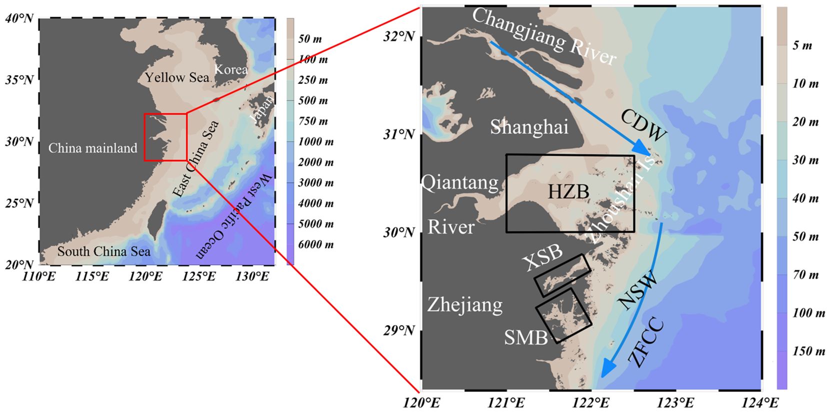
Figure 1. Map of the northern Zhejiang nearshore showing the study area. Areas framed with black solid lines indicate the three bays (including Hangzhou Bay (HZB), Xiangshan Bay (XSB) and Sanmen Bay (SMB)) categorized in this study to better constrain the spatial and temporal variability in CO₂ fluxes. The sea areas within the frames are the sea surface areas of XSB and SMB. Blue arrows indicate the direction of the Zhejiang-Fujian Coastal Current (ZFCC) and Changjiang Diluted Water (CDW).

The hydrological structure of the study area is primarily influenced by the East Asian monsoon. Long-term observations indicate that the Changjiang River plume flows southwestward along the coastline in winter, with a strong Zhejiang-Fujian coastal current (ZFCC), while it shifts northeastward in summer under the influence of the southeast monsoon (Bai et al., 2014). HZB, XSB, and SMB are the major estuarine bays in the northern coastal region of Zhejiang Province, each with relatively distinct geographical features. The study area is divided into HZB, XSB, SMB, and NSW (Figure 1).

HZB, a funnel-shaped macrotidal estuary characterized as a typical trumpet-shaped bay with strong tidal forces is the only estuarine bay in Zhejiang. The Qiantang River’s modest discharge (1.98×10¹⁰ m³ yr^-1) is overwhelmed by Changjiang-derived freshwater intrusions, creating a turbidity maximum zone (suspended sediment concentration: 0.3-1.0 kg m^-3) where light limitation suppresses phytoplankton blooms despite high nutrient availability (Li et al., 2025).

XSB, a narrow, semi-enclosed embayment (391 km², 10–15 m depth) that serves as Ningbo’s primary aquaculture hub. The XSB is influence by two local rivers, named by Fuxi stream and Yangonghe stream, with a discharge of about 1.30 km³ yr^-1 (Gao et al., 1990). Due to its elongated shape and weak hydrodynamic conditions, XSB has a relatively long water exchange cycle with the open sea (residence time >30 days) (Han et al., 2024; Sun et al., 2024). Chronic eutrophication, coupled with low suspended solids loads (0.025 kg m^-3), favors recurrent algal blooms.

SMB, the second-largest Zhejiang bay (775 km², ~9 m depth) features a multi-channel morphology connecting to the ECS through Shipu Harbor. Unlike neighboring systems, it lacks major river inputs (annual runoff: 2.68 km³), resulting in marine-dominated hydrochemistry. Its high natural suspended solids loads (0.367 kg m^-3) sustained by strong tidal resuspension and its relatively shallow depth (Li et al., 2024).

As shown in Figure 1, XSB and SMB are semi-enclosed bays with well-defined geographical boundaries. Therefore, the rectangular frames used in our study were delineated based on these geographical boundaries. HZB is an open estuarine bay, separated from NSW by the Zhoushan Islands. Based on this geographical feature, we delineated the boundary between HZB and NSW in our study. The division of our data is also based on the regional boundaries established in our study. The water areas within the frames represent the exact regions discussed in this paper.

2.2 Data acquisition

Seasonal underway surveys were conducted in Spring, summer, autumn by the “Zhejiang Environmental Monitoring 001” and in winter by the “Zhedaiyuyun 09911” vessel in 2024. Zhejiang Environmental Monitoring 001 is a marine ecological environment monitoring vessel. Zhedaiyuyun 09911 is a fishing transport vessel. Detailed information about the underway observation and the vessels are presented in Table 1. There were no significant meteorological conditions observed around the date of observation. Surface seawater and air pCO₂ were measured using a non-dispersive infrared spectrometer (LI-COR, LI-7000) integrated in an automated underway pCO₂ measuring system (General Oceanics, GO8050), which is commonly used on ships (Pierrot et al., 2009; Guo et al., 2015; Zhai and Dai, 2009). Surface seawater was continuously pumped from ~2 m depth and CO₂ mole fraction (xCO₂) was determined after air–water equilibration at about 2-min intervals. Air was pumped from a bow intake located at the prow of the vessel ~10 m above the water surface and xCO₂ in the air was measured at 2-h intervals. The barometric pressure was measured continuously onboard with a barometer fixed ~10 m above the sea surface. A series of CO₂ gas standards (provided by National Institute of Metrology, China) with xCO₂ values of 200, 298, 500 and 996 ppmv (parts per million volumes) were used to calibrate LI-7000. SST, SSS, DO and Chl-a were measured simultaneously with CO₂, using SBE45, Aanderaa 3835, and Seapoint Chlorophyll Fluorometer, respectively.

Table 1

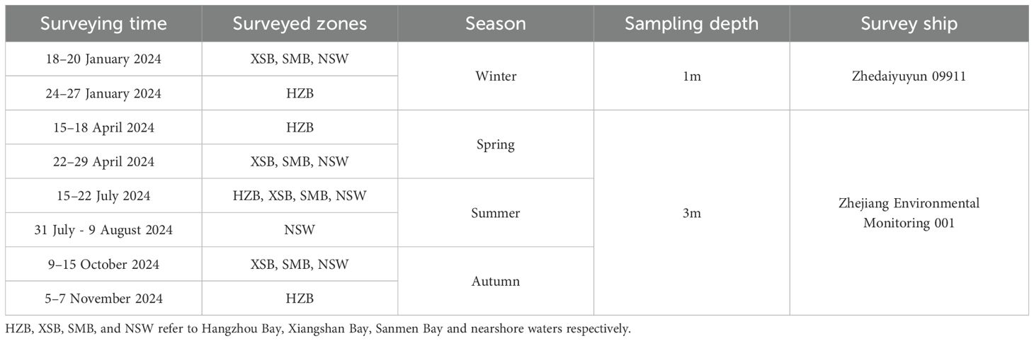
Table 1. Summary information of the 4 sampling surveys in 2024.

The spatial resolution of the wind speed data is 0.25°×0.25°, and the temporal resolution is one month. The seasonal averages were calculated for use in the wind speed computations. The wind speed data were obtained from the Environmental Research Division Data Access Program (ERDDAP, https://coastwatch.noaa.gov/erddap/index.html).

2.3 Data processing

The data processing follows the method of Pierrot et al. (2009). The pCO₂ in the equilibrator ($p{\text{CO}}_2^{Eq}$) is calculated through $x{\text{CO}}_2$ (the molar fraction of CO₂ in the gas measured by LI-7000, in units of ppm), with the specific formula (Equation 1) given by Weiss and Price (1980):

$\begin{array}{ll}p{\text{CO}}_2^{Eq}=(P_{Eq}-P_{H_{2}O})\times x{\text{CO}}_2& (1)\end{array}$

Where $p{\text{CO}}_2^{Eq}$ is the partial pressure of CO₂ in the equilibrator; $P_{Eq}$ is the saturation water vapor pressure; $P_{H_{2}O}$ is a function related to temperature and salinity, which can be calculated from the data obtained by the temperature and salinity sensors in the equilibrator. The atmospheric CO₂ was calculated similarly using xCO₂ in the air and the barometric pressure.

The pCO₂ in situ seawater ($In situ p{\text{CO}}_2$) was calculated using the empirical formula (Equation 2) provided by Takahashi et al. (1993):

$\begin{array}{ll}In situ p{\text{CO}}_2=p{\text{CO}}_2^{Eq}\times e^{(\text{SST}-t)\times 0.0423}& (2)\end{array}$

Where SST is the in situ seawater temperature; t is the temperature of the seawater in the equilibrator.

The normalization of temperature in this study was also calculated using the empirical formula (Equation 3) of Takahashi et al. (1993):

$\begin{array}{ll}n-p{\text{CO}}_2=In situ p{\text{CO}}_2\times e^{(20.0-\text{SST})\times 0.0423}& (3)\end{array}$

During the entire investigation period, the average SST was 19.6 °C. We used 20.0 °C for the normalization of pCO₂ calculations.

The air-sea CO₂ flux ($F_{{\text{CO}}_2}$) was calculated using the air-sea flux formula proposed by Liss (1973), based on the difference in pCO₂ between seawater and the atmosphere ($\text{Δ}p{\text{CO}}_2$) and the gas transfer velocity. When $F_{{\text{CO}}_2}$ is positive, it indicates that the study area acts as a source of CO₂, releasing CO₂ into the atmosphere. Conversely, when $F_{{\text{CO}}_2}$ is negative, it indicates that the study area acts as a sink for CO₂, absorbing CO₂ from the atmosphere. The specific formula (Equation 4) for calculating the air-sea CO₂ flux is as follows:

$\begin{array}{ll}{F}_{{\text{CO}}_2}=k\times K_H\times \text{Δ}p{\text{CO}}_2& (4)\end{array}$

Where $K_H$ is the solubility of CO₂ (Weiss, 1974); $\text{Δ}p{\text{CO}}_2$ is the pCO₂ difference between the surface water and the atmosphere; and k is the CO₂ transfer velocity, which was parameterized using the empirical function (Equations 5, 6) from Wanninkhof (1992) and Jiang et al. (2008):

$\begin{array}{ll}k=fc\times {\text{C}}_2\times U_{mean}^2\times {(S_C/660)}^{-0.5}& (5)\end{array}$

$\begin{array}{ll}{\text{C}}_2=\left(\frac{1}{n}\sum _{j=1}^n{U}_j^2\right)/U_{mean}^2& (6)\end{array}$

Where fc is a proportional coefficient (=0.27 in this study); $U_{mean}$ is the monthly wind speed at 10 m above sea; $S_C$ is the Schmidt number for CO₂ in seawater; $U_j$ is the high-frequency wind speed; the subscript “mean” indicates the average; and n is the number of available wind speeds in a month. ${\text{C}}_2$ is the nonlinear coefficient for the quadratic term of the gas transfer relationship. This coefficient accounts for the non-linear relationship between wind speed and gas transfer velocity under the assumption that long-term wind distributions follow a Rayleigh (Weibull) probability pattern. The empirical formula for CO₂ transfer velocity was established by Wanninkhof (1992). This formulation was derived by reconciling gas transfer velocity over the global ocean, which were determined by the natural-¹⁴C disequilibrium and the bomb-¹⁴C inventory methods. In the 1992 study, the proportional coefficient fc was calibrated as 0.31. Building upon the work of Wanninkhof (1992); Sweeney et al. (2007) recalculated the ocean inventory of bomb-¹⁴C in the global ocean and yielded an optimized fc value of 0.27. In this study, we adopt fc as 0.27 for the calculation of air-sea CO₂ fluxes. This choice aligns with recent regional applications in the East China Sea, where this coefficient has been validated through multiple field campaigns (Guo et al., 2015; Liu et al., 2019; Wu et al., 2021).

3 Results

3.1 SST and SSS

The study area is influenced by the East-Asian monsoon with distinct seasons (Zhai et al., 2014), exhibits significant seasonal and spatial variations in both temperature and salinity (Figure 2). Detailed statistical data on SST and SSS for each region across the four seasons are provided in Table 2. In winter, SST was the lowest, with an overall range of 6.19 to 12.87°C. There was little variation within each region, with HZB having the lowest SST (average 7.48 ± 0.69°C), while the southern regions had relatively higher SST, all exceeding 11°C on average. In spring, SST ranged from 13.67 to 20.44°C. HZB had the lowest SST, averaging 15.15 ± 0.88°C, while XSB and SMB had higher averages of 18.33 ± 1.02°C and 19.58 ± 0.64°C, respectively. NSW had an average SST of 16.97 ± 1.31°C. Summer SST were the highest of the year, ranging from 24.76 to 31.66°C. SMB had the highest SST, averaging 30.52 ± 0.77°C. In autumn, the average SST in HZB was 20.32 ± 0.43°C, significantly lower than in other regions (Figure 2a). This may be attributed to the fact that the field survey in HZB was conducted from November 5-7, approximately 20 days later than the surveys in the southern regions. These findings highlight the pronounced seasonal variability in the study area.

Figure 2

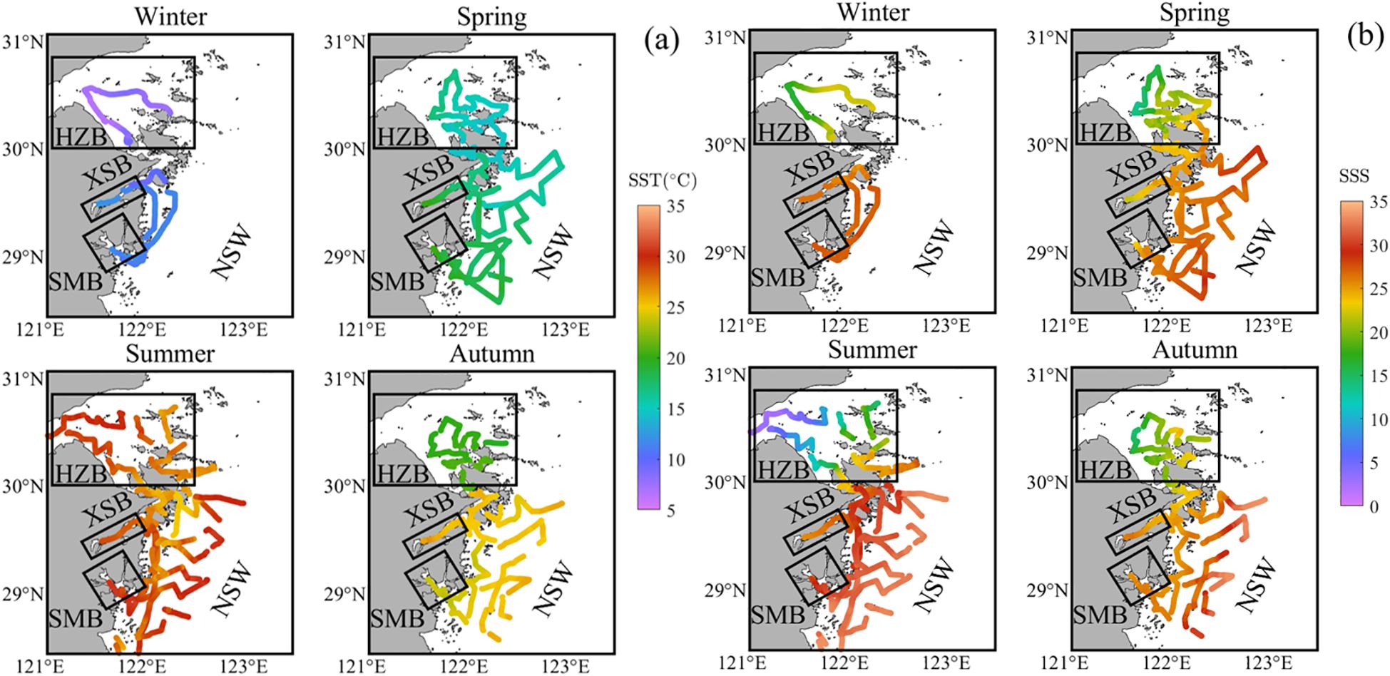
Figure 2. Seasonal distribution in the northern Zhejiang nearshore based on surveys from 2024: (a) sea surface temperature (SST) and (b) sea surface salinity (SSS). The framed areas show the three bays (including Hangzhou Bay (HZB), Xiangshan Bay (XSB) and Sanmen Bay (SMB)). The remaining area is divided into nearshore waters (NSW).

Table 2

Table 2. Data summary.

SSS generally exhibited the characteristic of being lower in HZB than in the southern regions and lower in nearshore areas than in offshore areas across all seasons (Figure 2b). In HZB, SSS showed a gradual increase from the Qiantang River estuary toward the ECS throughout the year. The lowest SSS occurred in summer, with an average of 13.28 and significant variability (SD = 7.59) which was primarily controlled by the high river discharge of the Changjiang River during this period (Bai et al., 2014). In the other three seasons, SSS averaged around 20. In XSB, SSS ranged from 21.77 to 27.42 across the four seasons. The lowest SSS occurred in spring, averaging 23.68 ± 0.96, while winter and summer had higher SSS values, averaging 26.38 ± 0.28 and 26.29 ± 0.51, respectively. Seasonal variability within XSB was minimal, and the spatial distribution was relatively consistent. In SMB, SSS ranged from 23.28 to 30.92, showing a similar seasonal pattern with XSB. The lowest SSS occurred in spring, averaging 24.80 ± 0.95, while winter and summer had higher SSS values, averaging 27.27 ± 0.14 and 28.82 ± 1.46, respectively. In NSW, SSS ranged from 21.80 to 33.40 across the four seasons. The highest SSS occurred in summer, averaging 30.53 ± 2.19, while the other three seasons had similar averages, around 26.80.

3.2 DO and Chl-a

During the entire investigation period, the DO saturation fluctuated within a range of 82 to 214%, indicating an overall near-saturation equilibrium state (Table 2). Spatially, as shown in Figure 3a, in winter, DO saturation showed little variation overall, with a high DO saturation value observed only at inner XSB (105 ± 7%). In spring, DO saturation generally increased from the inner bays toward the offshore areas, with noticeable supersaturation occurring in some offshore regions. In summer, DO saturation exhibited strong spatial heterogeneity. Supersaturated DO saturation were observed not only NSW (113 ± 24%) but also in XSB (114 ± 5%) and HZB (102 ± 10%). In autumn, DO saturation was relatively evenly distributed across the study area, with most regions close to saturation except for HZB, where DO saturation was relatively lower (92 ± 2%).

Figure 3

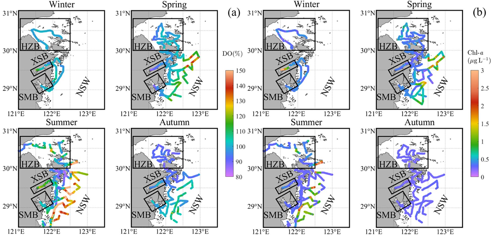
Figure 3. Seasonal distribution in the northern Zhejiang nearshore based on surveys from 2024: (a) DO saturation (DO%) and (b) chlorophyll-a (Chl-a). The framed areas show the three bays (including Hangzhou Bay (HZB), Xiangshan Bay (XSB) and Sanmen Bay (SMB)). The remaining area is divided into nearshore waters (NSW).

Chl-a concentrations exhibited high values in localized regions, such as XSB during winter, NSW during spring and summer, and HZB during summer. As shown in Figure 3, these high Chl-a regions generally coincided with areas of supersaturated DO saturation. This was likely due to favorable conditions for phytoplankton growth in these localized regions, leading to increased Chl-a and DO saturation through photosynthesis. In other regions and seasons, Chl-a concentrations remained at relatively low with minimal variability (Figure 3b).

3.3 Sea surface pCO₂ and air pCO₂

In the four study regions, sea surface pCO₂ measurements fluctuated within the range of 194 to 739 μatm, with above 70% of all underway data in this study concentrated in the range of 429 to 612 μatm (Figure 4). The study area generally acts as an atmospheric CO₂ source, which was consistent with previous research findings in similar regions (Liu et al., 2019; Yu et al., 2013). Specifically, the annual average pCO₂ was highest in SMB (555 ± 92 μatm), followed by HZB (533 ± 77 μatm), and was lowest in XSB (506 ± 112 μatm). However, all estuarine bays had significantly higher pCO₂ compared to the NSW (478 ± 76 μatm) (Table 2).

Figure 4

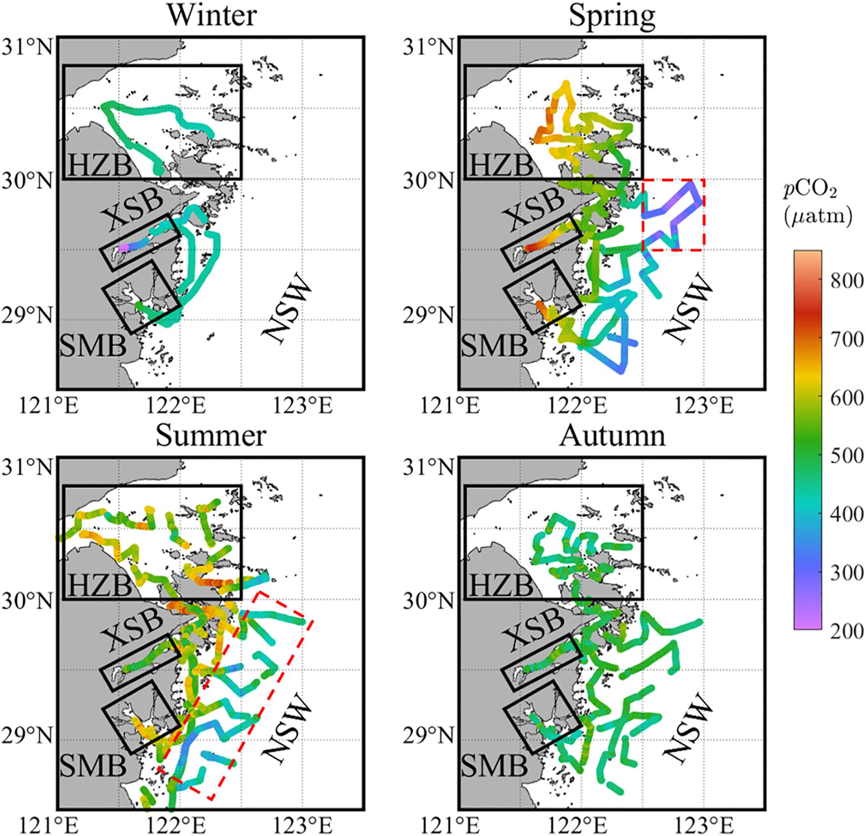
Figure 4. Seasonal distribution of surface water pCO₂ in the northern Zhejiang nearshore based on surveys from 2024. The black framed areas show the three bays (including Hangzhou Bay (HZB), Xiangshan Bay (XSB) and Sanmen Bay (SMB)). The remaining area is divided into nearshore waters (NSW). The red dotted border represents the area in NSW that is significantly affected by biological activity.

In HZB, the average pCO₂ in spring and summer exceeded 590 μatm, which was slightly lower than the values reported in earlier summer investigations in this area (618 μatm) (Yu et al., 2013). In autumn, the average pCO₂ was 481 ± 33 μatm, while in winter, it was the lowest at 453 ± 18 μatm. Notably, as shown in Figure 4, although overall pCO₂ in summer were relatively high, they exhibited significant spatial heterogeneity, with the lowest value reaching 428 μatm, which was consistent with previous studies that discovered the strongest temporal heterogeneity during summer (Liu et al., 2019).

In XSB, the pCO₂ in winter decreased to 367 ± 83 μatm, making it the only season in the four study regions where the area acts as an atmospheric CO₂ sink. The pCO₂ in XSB exhibited distinct seasonal variations, with the highest values in spring at 639 ± 52 μatm, significantly decreasing to 527 ± 36 μatm in summer, and further dropping to 491 ± 36 μatm in autumn.

The seasonal variations in pCO₂ in SMB exhibit a similar trend to those observed in HZB. The averaging pCO₂ in spring (653 ± 41 μatm) and summer (630 ± 23 μatm) were relatively high across the entire study region. In contrast, the averaging pCO₂ in autumn (472 ± 36 μatm) and winter (465 ± 17 μatm) were much lower.

In NSW, the seasonal variations in pCO₂ differed significantly from those observed in the estuarine bays. In winter, the average pCO₂ was 434 μatm, approaching the atmospheric pCO₂. In spring, pCO₂ rose to 456 μatm, with a notable increase in spatial heterogeneity (Figure 4), as the standard deviation increased significantly (9 μatm in winter, 93 μatm in spring). In summer, pCO₂ continued to rise, reaching to 532 ± 89 μatm, while maintaining a high spatial variability. In autumn, pCO₂ decreased, with an average of 489 ± 31 μatm.

In terms of spatial distribution (Figure 4), minimal spatial variation in pCO₂ was observed during winter, except in XSB. In spring and summer, pCO₂ generally decreased gradually from the inner estuary to the offshore regions. In autumn, pCO₂ were relatively consistent across the study area, averaging around 490 μatm.

During the entire investigation period, atmospheric pCO₂ fluctuated within the range of 397-434 μatm. The highest pCO₂ were typically observed during winter, while the lowest pCO₂ were recorded in summer. Overall, the average atmospheric pCO₂ in HZB was the highest at 423 ± 7 μatm, higher than those in the other regions (417-419 μatm).

3.4 Wind speed

The study area is influenced by the southeast monsoon, characterized by low wind speeds in spring and summer, and the northwest monsoon, characterized by high wind speeds in autumn and winter. This results in overall lower wind speeds in spring and summer compared to autumn and winter (Cao et al., 2023). The annual wind speed ranged from 1.4 to 10.0 m s^-1, with an average of 5.4 ± 1.8 m s^-1. Seasonally, all regions exhibited the highest wind speeds in autumn, followed by winter, while spring and summer had relatively lower wind speeds (Table 2). In terms of intra-seasonal variability, autumn and winter showed greater fluctuations, with standard deviations (SD) ranging from 0.7 to 1.6 m s^-1, while spring and summer had significantly lower variability, with SD of 0.4 to 0.9 m s^-1. Spatially, NSW had the highest annual average wind speed at 5.9 m s^-1, significantly higher than the three estuarine bays. XSB had the lowest annual average wind speed at 2.7 m s^-1, while HZB and SMB had annual average wind speeds of 4.7 m s^-1 and 4.9 m s^-1, respectively.

In this study C₂ ranged from 1.14 to 1.57. The annual average C₂ in HZB, XSB, SMB and NSW was 1.23 ± 0.12, 1.33 ± 0.16, 1.28 ± 0.07 and 1.26 ± 0.08, respectively. The total annual average C₂ (1.28) was similar to the global average of 1.27 (Wanninkhof, 2014).

3.5 Air-sea CO₂ flux

As shown in Table 2, the annual average air-sea CO₂ flux in the four study regions exhibited significant spatial differences. XSB had the lowest flux, with an annual average of 1.2 ± 2.3 mmol m^-2 d^-1. NSW followed, with an annual average flux of 5.2 ± 5.9 mmol m^-2 d^-1. HZB and SMB exhibited the higher flux, functioning as moderate sources with annual averages of 6.0-7.0 mmol m^-2 d^-1.

In the seasonal variations, the average flux among the three estuarine bays gradually increased from winter to spring. However, the overall flux showed relatively small changes in spring, summer and autumn. In contrast, NSW displayed a distinct pattern of seasonal variation. During the transition from winter to spring, NSW maintained a relatively weak source, with little difference in flux (1.4 mmol m^-2 d^-1 in winter, 1.8 mmol m^-2 d^-1 in spring). During the transitions from spring to summer and from summer to autumn, NSW experienced a significant increase in the average flux. Specifically, the summer flux averaged 6.4 ± 4.5 mmol m^-2 d^-1, while the autumn flux further increased to 11.4 ± 4.6 mmol m^-2 d^-1.

4 Discussion

4.1 Controls on sea surface pCO₂

Surface water pCO₂ in coastal ocean is influenced not only by temperature, mixing processes, tidal dynamics, and biological activities, but also by terrestrial factors such as riverine discharges (Gruber, 2015; Mathis et al., 2024). Within the carbonate thermodynamic system, temperature exerts a significant control, with each 1°C change altering surface seawater pCO₂ by approximately 4.23% (Takahashi et al., 1993). This thermodynamic dependency explains why temperature has been consistently identified as the dominant factor governing seasonal pCO₂ variations in previous studies (Liu et al., 2019; Li et al., 2020; Zhai et al., 2013). Our four-season investigation revealed a pronounced temperature gradient, with the maximum seasonal difference exceeding 20°C between summer and winter. To decouple the thermal and non-thermal drivers of pCO₂ variability, we implemented a dual analytical approach: 1) analysis of in situ measured pCO₂ and 2) evaluation of temperature-normalized pCO₂ (n-pCO₂) calculated using 20.0°C as the reference baseline.

In the open oceans, seasonal variations in pCO₂ are primarily governed by temperature, following characteristic thermal curves. However, coastal systems exhibit more complex controls, where pCO₂ dynamics often deviate from temperature-driven patterns due to multiple interacting factors (Wu et al., 2021; Liu et al., 2019). As shown in Figures 5a, f, k, p, the relationship between pCO₂ and temperature in the study areas demonstrates this decoupling phenomenon. To quantify temperature-independent effects, we defined the lower and upper bounds of thermally controlled pCO₂ using the summer-autumn n-pCO₂ ranging from 350 to 500 μatm observed in offshore waters as reference thresholds.

Figure 5

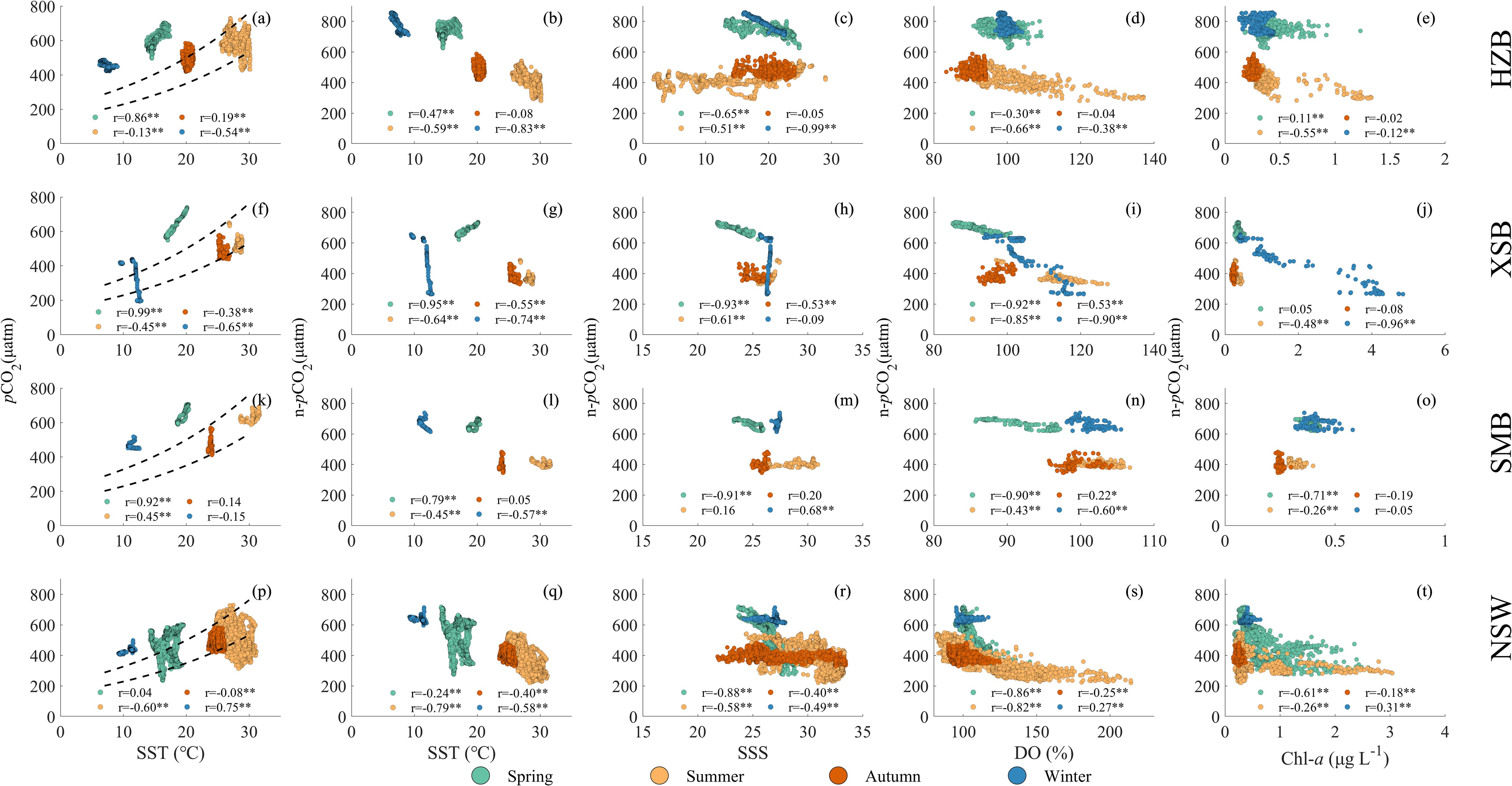
Figure 5. Relationships of (a, f, k, p) sea surface water pCO₂ with sea surface temperature (SST); (b, g, l, q) n-pCO₂ (pCO₂ normalized to 20.0°C) with SST; (c, h, m, r) n- pCO₂ with sea surface salinity (SSS); (d, i, n, s) n- pCO₂ with dissolved oxygen saturation (DO(%)); (e, j, o, t) n- pCO₂ with chlorophyll a (Chl-a). The first row of panels represents the Hangzhou Bay (HZB), the second row represents the Xiangshan Bay (XSB), the third row represents the Sanmen Bay (SMB), and the fourth row represents the nearshore waters (NSW). The dashed lines in the first column indicate 350 × exp((SST - 20.0) × 0.0423) and 500 × exp((SST - 20.0) × 0.0423) µatm (see details in the text).

In HZB, previous estuarine studies have demonstrated that this region exhibits elevated pCO₂ due to the influence of high-pCO₂ riverine inputs from the Changjiang and Qiantang Rivers (Zhai et al., 2007; Gao et al., 2008). The lowest pCO₂ (453 ± 18 μatm) was observed in winter, primarily controlled by low temperatures (average 7.48°C), with limited variability (Table 2). In spring, as SST increased to 15.15°C, pCO₂ rose to 603 μatm (Table 2). An increase in temperature by 1°C would result in a 4.23% rise in pCO₂ according to the thermal effect. Thus temperature elevation contributed 174 μatm to this pCO₂ increase if no other factors was considered. The contribution of temperature elevation to the increase in pCO₂ exceeded the actual change value (150 μatm), indicating that other factors offset part of the influence brought by the temperature change. Both winter and spring pCO₂ exceeded the temperature-predicted levels (Figure 5a), suggesting additional CO₂ inputs. The observed negative correlation between n-pCO₂ and SSS during these seasons implies horizontal mixing processes (Figure 5c), consistent with buoy observations in HZB (Liu et al., 2019). This horizontal mixing is identified as the primary driver of elevated pCO₂ in spring and winter. Spatial distribution in Figure 4 demonstrated the higher pCO₂ values in the areas adjacent to freshwater sources. During summer and autumn, no significant correlations were observed between pCO₂ and SST or between n-pCO₂ and SSS (Figures 5a, c), though pCO₂ generally followed temperature-predicted trends. From spring to summer, as SST increased from 15.15°C to 28.28°C, the theoretical temperature-driven pCO₂ rise (calculated using the 4.23% °C^-1 coefficient) would amount to approximately 448 μatm. However, the measured pCO₂ decreased slightly from 603 μatm to 593 μatm. This discrepancy was attributed to summer stratification, which reduced vertical mixing and limited pCO₂ accumulation at the surface. A negative correlation between summer n-pCO₂ and both DO saturation and Chl-a suggests localized biological CO₂ uptake (Figures 5d, e). Notably, the lowest pCO₂ values associated with high biological activity predominantly occurred during neap tides (July 16, 2024). In autumn, no significant correlations were found between n-pCO₂ and DO saturation or Chl-a (Figures 5d, e). The summer-to-autumn transition was dominated by thermal effects, accounting for 170 μatm reduction in pCO₂ variation due to cooling. Conversely, from autumn to winter, despite a 12.84°C temperature decrease, n-pCO₂ increased from 475 μatm to 770 μatm (Table 2). This counter-thermal trend reflects substantial non-thermal CO₂ inputs, primarily driven by horizontal mixing of high-CO₂ freshwater plumes from riverine sources.

In XSB, similar to HZB, pCO₂ in winter and spring exceeded temperature-predicted values, with n-pCO₂ showing negative correlations with SSS (excluding biological effects) (Figures 5f, h). Distinctively, pronounced biological absorption was observed in the innermost part of the bay during winter underway survey (Figure 4), evidenced by elevated DO saturation and Chl-a inversely related to pCO₂ (Figures 5i, j). This biological drawdown reduced pCO₂ to a minimum of 194 μatm, temporarily converting the area into a carbon sink. This biological absorption was attributed to relatively higher winter temperatures and weakened water exchange in the innermost part of the bay (Sun et al., 2024), conditions conducive to phytoplankton growth (Zhang et al., 2012). These favorable conditions led to the observed high Chl-a values in winter, as shown in Figure 3b. During the same period, the changes in SST and SSS were limited, which led to form a vertically aligned straight line in the Figures 5f–h. From winter to spring, as average SST increased from 10.97°C to 18.33°C, pCO₂ rose from 430 μatm (excluding low value points affected by biological effects) to 639 μatm. Thermal effects accounted for 75% of this increase, while the residual 25% variability correlated with horizontal mixing processes, as indicated by the negative relationship between n-pCO₂ and SSS (Figures 5f, h). During summer and autumn (Figure 5f), pCO₂ dynamics aligned with thermal predictions, showing no significant correlations with other parameters. Notably, summer-autumn n-pCO₂ were systematically lower than winter-spring values, reflecting intensified stratification that inhibited vertical mixing of high-pCO₂ deep waters. No significant biological activity was detected during summer-autumn surveys, with minimal n-pCO₂ variability observed throughout these seasons.

In SMB, also similar to HZB, winter and spring pCO₂ exceeded temperature-predicted values, with spring n-pCO₂ exhibiting a negative correlation with SSS (Figures 5k, m). During summer and autumn, pCO₂ dynamics aligned closely with thermal predictions, showing no significant correlations with other parameters. Seasonal variability was minimal, likely attributable to well-mixed water column conditions. No pronounced biological activity was observed throughout the year, consistent with the region’s persistently high turbidity (Gao et al., 2022). Both winter and spring n-pCO₂ in SMB were influenced by horizontal mixing processes, with nearly identical values of 668 μatm (winter) and 664 μatm (spring). Similarly, summer and autumn n-pCO₂ remained stable at 404 μatm and 401 μatm, respectively. Seasonal transitions between winter-spring and summer-autumn were predominantly governed by thermal effects. The spring-to-summer period showed a 260 μatm decrease in n-pCO₂, primarily driven by weakened vertical mixing. Conversely, a 267 μatm increase in n-pCO₂ from autumn to winter reflected enhanced horizontal mixing of high-CO₂ water masses.

In NSW, pCO₂ patterns align with temperature-predicted curves (Figure 5p), though intra-seasonal variability was pronounced, likely due to the extensive spatial coverage of the study area. Seasonal analysis reveals elevated pCO₂ above thermal predictions during winter and partially in spring, with the negative n-pCO₂ with SSS indicating horizontal mixing influences. Summer pCO₂ partially fell below the thermal curve, while autumn pCO₂ largely adhered to temperature-driven expectations. The values below the temperature curve were mainly due to the influence of biological effects. As can be seen from Figures 5s, t, n-pCO₂ was negatively correlated with DO saturation and Chl-a overall. Most of the low values of n-pCO₂ correspond to high values of DO saturation and Chl-a, especially the negative correlation with DO was more significant, which can reflect the biological role. Previous studies suggest biological production predominantly controls surface pCO₂ dynamics on the ECS inner shelf (Chou et al., 2013; Mathis et al., 2024). In this study, localized biological activity occurred only in spring and summer, primarily in offshore areas (Figure 4), where reduced turbidity facilitated phytoplankton growth. These regions exhibited markedly higher DO saturation and Chl-a, coupled with pCO₂ below atmospheric equilibrium, forming distinct carbon sinks. Thermal forcing remained dominant across seasonal transitions, accounting for 122 μatm (winter-to-spring), 270 μatm (spring-to-summer), 63 μatm (summer-to-autumn), and 217 μatm (autumn-to-winter) of pCO₂ variability. Beyond biological effects, winter-spring n-pCO₂ significantly exceeded summer-autumn, reflecting intensified horizontal mixing of terrestrial-sourced high-CO₂ waters during colder seasons.

The study area exhibits distinct spatial and seasonal variations in surface seawater pCO₂. Biological activity exerts localized impacts on pCO₂ reduction, particularly in XSB during winter and specific offshore areas in spring-summer, forming temporary carbon sinks. Excluding biological effects, winter pCO₂ minima was thermally driven, while elevated spring and summer pCO₂ were primarily attributed to horizontal mixing and temperature increases, respectively. Seasonally, n-pCO₂ remains significantly higher in winter and spring than those in summer and autumn, with horizontal mixing identified as the dominant driver. Summer n-pCO₂ minima reflect dual controls: sustained phytoplankton consumption reduces pCO₂, while stratification limits vertical mixing of high-CO₂ deep waters.

4.2 Seasonal variation of air-sea CO₂ flux

The direction of air-sea carbon flux is determined by the sign of ΔpCO₂ (the pCO₂ difference between the surface water and the atmosphere), while its magnitude depends on the gas transfer velocity, ΔpCO₂, and wind speed (Chen et al., 2013).

Atmospheric pCO₂ in the study area exhibited limited seasonal variation (397-434 μatm), contrasting with seawater pCO₂ ranging from 194 to 739 μatm. Negative ΔpCO₂ occurred exclusively in XSB during winter, marking it as a CO₂ sink. All other regions and seasons acted as CO₂ sources. Wind speeds were significantly higher in autumn and winter than those in spring and summer, with XSB exhibiting consistently lower wind speeds compared to the other areas.

The CO₂ flux in HZB ranged from -0.5 to 16.2 mmol m^-2 d^-1, with an annual mean of 6.0 ± 3.7 mmol m^-2 d^-1 (Figure 6c), indicating consistent CO₂ emissions across all seasons. In HZB, the CO₂ flux obtained in this study (6.0 ± 3.7 mmol m^-2 d^-1) was lower than that reported in previous research (14.0 ± 9.0 mmol m^-2 d^-1) which was based on buoy data collected during winter, spring, and summer (Liu et al., 2019). Seasonal flux minima occurred in winter (1.6 ± 1.2 mmol m^-2 d^-1), driven by low ΔpCO₂ of 24 μatm, while maxima peaked in spring (9.2 ± 2.2 mmol m^-2 d^-1). As shown in Figures 6a, b, Wind speeds were notably higher in autumn compared to other seasons, yet the concurrent lower ΔpCO₂ (180 μatm in spring and summer; 63 μatm in autumn) counterbalanced this forcing, resulting in no significant flux elevation.

Figure 6

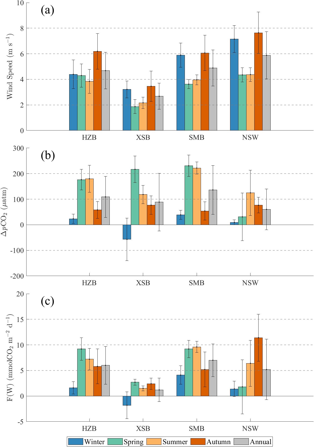
Figure 6. Seasonal variations of (a) Wind Speeds, (b) ΔpCO₂, and (c) air-sea CO₂ fluxes in the four study regions. The error bars are the standard deviations. HZB, XSB, SMB, and NSW refer to Hangzhou Bay, Xiangshan Bay, Sanmen Bay and nearshore waters respectively.

The CO₂ flux in XSB ranged from -7.2 to 5.2 mmol m^-2 d^-1, with an annual mean of 1.2 ± 2.3 mmol m^-2 d^-1 (Figure 6c). The region acted as a CO₂ sink during winter (-1.8 ± 2.6 mmol m^-2 d^-1) but served as a source in other seasons. As shown in Figure 6a, persistently low wind speeds in XSB limited flux magnitudes, even when spring ΔpCO₂ reached 217 μatm. Based on the bay’s area of 391 km² (Figure 1), annual CO₂ emissions totaled 2.1×10⁹ g C, while winter CO₂ uptake amounted to 0.8×10⁹ g C.

The CO₂ flux in SMB ranged from -0.6 to 14.6 mmol m^-2 d^-1, with an annual mean of 7.0 ± 3.2 mmol m^-2 d^-1 (Figure 6c). As shown in Figures 6a, b, higher wind speeds in autumn and winter (~6.0 m s^-1) coincided with lower ΔpCO₂ (54 μatm in autumn; 39 μatm in winter), while lower winds in spring and summer (~3.8 m s^-1) corresponded to elevated ΔpCO₂ (>220 μatm). Pronounced seasonal ΔpCO₂ gradients dominated flux variability, resulting in significantly higher fluxes in spring (9.2 ± 1.7 mmol m^-2 d^-1) and summer (9.6 ± 1.1 mmol m^-2 d^-1) compared to fluxes in autumn (5.2 ± 3.4 mmol m^-2 d^-1) and winter (4.1 ± 1.8 mmol m^-2 d^-1). With a surface area of 775 km² (Figure 1), SMB emitted 2.4×10¹⁰ g C annually.

The CO₂ flux in NSW ranged from -10.7 to 25.7 mmol m^-2 d^-1, with an annual mean of 5.2 ± 5.9 mmol m^-2 d^-1 (Figure 6c). As shown in Figure 6a, wind speeds in autumn and winter were significantly higher than those in spring and summer. Winter fluxes remained notably low due to minimal ΔpCO₂ (9 μatm), while autumn exhibited the highest fluxes, driven by peak wind speeds (7.6 m s^-1) and elevated ΔpCO₂ (77 μatm). In contrast to previous studies in the Changjiang River plume (Guo et al., 2015), which reported the area as a net CO₂ sink (-6.2 ± 9.1 mmol m^-2 d^-1), our study reveals that NSW which was closer to the land act as a net CO₂ source (5.2 ± 5.9 mmol m^-2 d^-1).

The study area predominantly acts as a net source of atmospheric CO₂ due to persistently elevated ΔpCO₂. While this research quantifies seasonal air-sea carbon flux variability in Zhejiang’s high-turbidity coastal waters, substantial intra-seasonal fluctuations likely persist, particularly during transitional periods (Liu et al., 2019; Li et al., 2019). The nutrient-replete coastal environment remains prone to episodic phytoplankton blooms under favorable conditions, which may abruptly alter surface pCO₂ and modulate CO₂ fluxes (Yu et al., 2022; Chen et al., 2012). Furthermore, frequent typhoon impacts during summer-autumn induce rapid hydrographic changes (e.g., mixed-layer deepening and vertical nutrient injection (Li et al., 2021, 2019; Yu et al., 2020), necessitating future investigations combining enhanced observational networks and coupled biogeochemical modeling to resolve typhoon-driven carbon dynamics.

5 Conclusions

Our investigation reveals pronounced spatiotemporal heterogeneity in sea surface pCO₂ and air-sea CO₂ flux across estuarine, bay, and nearshore environments in northern Zhejiang. The study region predominantly functions as an annual weak-to-moderate CO₂ source to the atmosphere, with the exception of XSB, which acted as a weak CO₂ sink during winter due to combined effects of low temperatures and enhanced biological uptake. Annual mean air-sea CO₂ fluxes demonstrated marked regional variability: HZB, 6.0 ± 3.7 mmol m^-2 d^-1; XSB, 1.2 ± 2.3 mmol m^-2 d^-1; SMB, 7.0 ± 3.2 mmol m^-2 d^-1; and NSW, 5.2 ± 5.9 mmol m^-2 d^-1. Seasonal analysis identified SST as the dominant control on pCO₂ spatial patterns, while winter and spring conditions revealed horizontal mixing enhanced CO₂ enrichment beyond thermal influences. In addition, other factors like biological activity, and turbidity also contributed to the pCO₂ variations. This study establishes northern Zhejiang’s estuarine-coastal complex as a net CO₂ source while elucidating key controlling mechanisms, providing critical insights for regional carbon budgeting and biogeochemical model parameterization. Future investigations should prioritize high-temporal-resolution monitoring coupled with multivariate analysis to disentangle interacting drivers and refine flux quantification in these environmentally sensitive coastal zones.

Data availability statement

The raw data supporting the conclusions of this article will be made available by the authors, without undue reservation.

Author contributions

ZY: Writing – original draft, Writing – review & editing, Data curation, Investigation. XY: Data curation, Investigation, Writing – review & editing. CZ: Methodology, Writing – review & editing. YJ: Investigation, Writing – original draft. XH: Writing – original draft. XZ: Writing – review & editing. TZ: Writing – original draft. JN: Investigation, Writing – review & editing. JZ: Funding acquisition, Writing – review & editing. PY: Funding acquisition, Writing – review & editing, Writing – original draft.

Funding

The author(s) declare that financial support was received for the research and/or publication of this article. This study was supported by Key R&D Program of Zhejiang (Grant No. 2023C03120 and 2023C03011), Natural Science Foundation of Zhejiang Province (Grant #LDT23D06021D06), and Science Foundation of Donghai Laboratory (Grant No. DH-2022KF0214).

Acknowledgments

The authors would like to thank the crews of the “Zhejiang Environmental Monitoring 001” and the “Zhedaiyuyun 09911” vessels for their help in field sampling.

Conflict of interest

The authors declare that the research was conducted in the absence of any commercial or financial relationships that could be construed as a potential conflict of interest.

Generative AI statement

The author(s) declare that no Generative AI was used in the creation of this manuscript.

Publisher’s note

All claims expressed in this article are solely those of the authors and do not necessarily represent those of their affiliated organizations, or those of the publisher, the editors and the reviewers. Any product that may be evaluated in this article, or claim that may be made by its manufacturer, is not guaranteed or endorsed by the publisher.

References

Bai Y., He X. Q., Pan D. L., Chen C.-T. A., Kang Y., Chen X. Y., et al. (2014). Summertime Changjiang River plume variation during 1998–2010. J. Geophys. Res.: Oceans 119, 6238–6257. doi: 10.1002/2014JC009866

Crossref Full Text | Google Scholar

Cai W. J. (2011). Estuarine and coastal ocean carbon paradox: CO₂ sinks or sites of terrestrial carbon incineration? Annu. Rev. Mar. Sci. 3, 123–145. doi: 10.1146/annurev-marine-120709-142723

PubMed Abstract | PubMed Abstract | Crossref Full Text | Google Scholar

Cao Z. Y., Wang J. K., He Q., Zhang X., Fu N., and Chen D. (2023). Analysis of the climatic characteristics and influence system of strong wind along the coast of Zhejian. Mar. Forecasts 40, 89–97. doi: 10.11737/j.issn.1003-0239.2023.02.009

Crossref Full Text | Google Scholar

Chen C.-T. A. and Borges A. V. (2009). Reconciling opposing views on carbon cycling in the coastal ocean: Continental shelves as sinks and near-shore ecosystems as sources of atmospheric CO₂. Deep-Sea Res. 56(8-10), 578–590. doi: 10.1016/j.dsr2.2009.01.001

Crossref Full Text | Google Scholar

Chen C.-T. A., Huang T.-H., Chen Y.-C., Bai Y., He X. Q., and Kang Y. (2013). Air-sea exchanges of CO₂ in the world’s coastal seas. Biogeosciences 10, 6509–6544. doi: 10.5194/bg-10-6509-2013

Crossref Full Text | Google Scholar

Chen C.-T. A., Huang T.-H., Fu Y.-H., Bai Y., and He X. Q. (2012). Strong sources of CO₂ in upper estuaries become sinks of CO₂ in large river plumes. Curr. Opin. Environ. Sustain. 4, 179–185. doi: 10.1016/j.cosust.2012.02.003

Crossref Full Text | Google Scholar

Chen C.-T. A., Zhai W. D., and Dai M. H. (2008). Riverine input and air–sea CO₂ exchanges near the Changjiang (Yangtze River) Estuary: Status quo and implication on possible future changes in metabolic status. Cont. Shelf Res. 28, 1476–1482. doi: 10.1016/j.csr.2007.10.013

Crossref Full Text | Google Scholar

Chou W. C., Gong G. C., Cai W. J., and Tseng C. M. (2013). Seasonality of CO₂ in coastal oceans altered by increasing anthropogenic nutrient delivery from large rivers: evidence from the Changjiang–East China sea system. Biogeosciences 10, 3889–3899. doi: 10.5194/bg-10-3889-2013

Crossref Full Text | Google Scholar

Chou W. C., Gong G. C., Tseng C. M., Sheu D. D., Hung C. C., Chang L. P., et al. (2011). The carbonate system in the East China Sea in winter. Mar. Chem. 123, 44–55. doi: 10.1016/j.marchem.2010.09.004

Crossref Full Text | Google Scholar

Dai M. H., Cao Z. M., Guo X. H., Zhai W. D., Liu Z. Y., Yin Z. Q., et al. (2013). Why are some marginal seas sources of atmospheric CO₂? Geophys. Res. Lett. 40, 2154–2158. doi: 10.1002/grl.50390

Crossref Full Text | Google Scholar

Dai M. H., Su J. Z., Zhao Y. Y., Hofmann E. E., Cao Z. M., Cai W. J., et al. (2022). Carbon fluxes in the coastal ocean: synthesis, boundary processes, and future trends. Annu. Rev. Earth Planet. Sci. 50, 593–626. doi: 10.1146/annurev-earth-032320-090746

Crossref Full Text | Google Scholar

Dai A. and Trenberth K. E. (2002). Estimates of freshwater discharge from continents: Latitudinal and seasonal variations. J. Hydrometeorol. 3, 660–687. doi: 10.1175/1525-7541(2002)003<0660:eofdfc>2.0.co;2

Crossref Full Text | Google Scholar

Deng X., Zhang G. L., Xin M., Liu C. Y., and Cai W. J. (2021). Carbonate chemistry variability in the southern Yellow Sea and East China Sea during spring of 2017 and summer of 2018. Sci. Total Environ. 779, 146376. doi: 10.1016/j.scitotenv.2021.146376

PubMed Abstract | PubMed Abstract | Crossref Full Text | Google Scholar

Fang Z., Feng T., Qin G. R., Meng Y. J. H., Zhao S. Y., Yang G., et al. (2024). Simulations of water pollutants in the Hangzhou Bay, China: Hydrodynamics, characteristics, and sources. Mar. pollut. Bull. 200, 116140. doi: 10.1016/j.marpolbul.2024.116140

PubMed Abstract | PubMed Abstract | Crossref Full Text | Google Scholar

Friedlingstein P., O’sullivan M., Jones M. W., Andrew R. M., Hauck J., Olsen A., et al. (2020). Global carbon budget 2020. Earth Syst. Sci. Data Discuss. 2020, 1–3. doi: 10.5194/essd-12-3269-2020

Crossref Full Text | Google Scholar

Gao S., Chun X. Q., and Jun F. Y. (1990). Fine-grained sediment transport and sorting by tidal exchange in Xiangshan Bay, Zhejiang, China. Estuar. Coast. Shelf Sci. 31, 397–409. doi: 10.1016/0272-7714(90)90034-o

Crossref Full Text | Google Scholar

Gao Y. X., Jiang Z. B., Chen Y., Liu J. J., Zhu Y. L., Liu X. Y., et al. (2022). Spatial variability of phytoplankton and environmental drivers in the turbid Sanmen bay (East China Sea). Estuar. Coasts 45, 2519–2533. doi: 10.1007/s12237-022-01104-7

Crossref Full Text | Google Scholar

Gao X. L., Song J. M., Li X. G., Li N., and Yuan H. M. (2008). PCO₂ and carbon fluxes across sea-air interface in the Changjiang Estuary and Hangzhou Bay. Chin. J. Oceanol. Limnol. 26, 289–295. doi: 10.1007/s00343-008-0289-8

Crossref Full Text | Google Scholar

Gruber N. (2015). Carbon at the coastal interface. Nature 517, 148–149. doi: 10.1038/nature14082

PubMed Abstract | PubMed Abstract | Crossref Full Text | Google Scholar

Guo X. H., Zhai W. D., Dai M. H., Zhang C., Bai Y., Xu Y., et al. (2015). Air–sea CO₂ fluxes in the East China Sea based on multiple-year underway observations. Biogeosciences 12, 5123–5167. doi: 10.5194/bg-12-5495-2015

Crossref Full Text | Google Scholar

Han Q. X., Wang X. B., and Xu Y. (2024). Deciphering macrobenthic biological traits in response to long-term eutrophication in Xiangshan Bay, China. Sci. Rep. 14, 20209. doi: 10.1038/s41598-024-71239-z

PubMed Abstract | PubMed Abstract | Crossref Full Text | Google Scholar

Jiang L. Q., Cai W. J., Wanninkhof R., Wang Y. C., and Lüger H. (2008). Air-sea CO₂ fluxes on the US South Atlantic Bight: Spatial and seasonal variability. J. Geophys. Res.: Oceans 113, C07019. doi: 10.1029/2007JC004366

Crossref Full Text | Google Scholar

Kim D., Choi S.-H., Shim J., Kim K.-H., and Kim C.-H. (2013). Revisiting the seasonal variations of sea-air CO₂ fluxes in the northern east China Sea. Terr. Atmos. Ocean. Sci. 24, 409–419. doi: 10.3319/tao.2012.12.06.01(OC

Crossref Full Text | Google Scholar

Laruelle G. G., Cai W.-J., Hu X., Gruber N., Mackenzie F. T., and Regnier P. (2018). Continental shelves as a variable but increasing global sink for atmospheric carbon dioxide. Nat. Commun. 9, 454. doi: 10.1038/s41467-017-02738-z

PubMed Abstract | PubMed Abstract | Crossref Full Text | Google Scholar

Li D. W., Chen J. F., Ni X. B., Wang K., Zeng D. Y., Wang B., et al. (2019). Hypoxic bottom waters as a carbon source to atmosphere during a typhoon passage over the East China Sea. Geophys. Res. Lett. 46, 11329–11337. doi: 10.1029/2019GL083933

Crossref Full Text | Google Scholar

Li Q., Guo X. H., Zhai W. D., Xu Y., and Dai M. H. (2020). Partial pressure of CO₂ and air-sea CO₂ fluxes in the South China Sea: Synthesis of an 18-year dataset. Prog. Oceanogr. 182, 102272. doi: 10.1016/j.pocean.2020.102272

Crossref Full Text | Google Scholar

Li J. D., Lai J. H., Duan Y., and Jiang Y. J. (2025). Conversion between suspended sediment concentration and turbidity of summer surface water in Zhejiang offshore area. Discov. Oceans 2, 5. doi: 10.1007/s44289-025-00042-z

Crossref Full Text | Google Scholar

Li D. W., Ni X. B., Wang K., Zeng D. Y., Wang B., Jin H. Y., et al. (2021). Biological CO₂ uptake and upwelling regulate the Air-Sea CO₂ flux in the Changjiang plume under south winds in summer. Front. Mar. Sci. 8. doi: 10.3389/fmars.2021.709783

Crossref Full Text | Google Scholar

Li L., Wu L. H., Yuan J. X., Zhao X. Y., and Xia Y. Z. (2024). Water environment in macro-tidal muddy Sanmen Bay. J. Mar. Sci. Eng. 13, 55. doi: 10.3390/jmse13010055

Crossref Full Text | Google Scholar

Liss P. S. (1973). Processes of gas exchange across an air-water interface. Deep Sea Res. Oceanogr. Abstracts 20, 221–238. doi: 10.1016/0011-7471(73)90013-2

Crossref Full Text | Google Scholar

Liu T. Y., Bai Y., Zhu B. Z., LI T., and Gong F. (2023). Satellite retrieval algorithm of high spatial resolution sea surface partial pressure of CO₂: Application of machine learning in Xiangshan Bay in autumn. J. Mar. Sci. 41, 82. doi: 10.3969/j.issn.1001-909X.2023.01.007

Crossref Full Text | Google Scholar

Liu J., Bellerby R. G., Li X. S., and Yang A. Q. (2022). Seasonal variability of the carbonate system and air–sea CO₂ flux in the outer Changjiang Estuary, East China Sea. Front. Mar. Sci. 8. doi: 10.3389/fmars.2021.765564

Crossref Full Text | Google Scholar

Liu Q., Dong X., Chen J. S., Guo X. H., and Dai M. H. (2019). Diurnal to interannual variability of sea surface pCO₂ and its controls in a turbid tidal-driven nearshore system in the vicinity of the East China Sea based on buoy observations. Mar. Chem. 216, 103690. doi: 10.1016/j.marchem.2019.103690

Crossref Full Text | Google Scholar

Liu Q., Guo X. H., Yin Z. Q., Zhou K. B., Roberts E. G., and Dai M. H. (2018). Carbon fluxes in the China Seas: An overview and perspective. Sci. China Earth Sci. 61, 1564–1582. doi: 10.1007/s11430-017-9267-4

Crossref Full Text | Google Scholar

Mathis M., Lacroix F., Hagemann S., Nielsen D. M., Ilyina T., and Schrum C. (2024). Enhanced CO₂ uptake of the coastal ocean is dominated by biological carbon fixation. Nat. Climate Change 14, 373–379. doi: 10.1038/s41558-024-01956-w

Crossref Full Text | Google Scholar

Pierrot D., Neill C., Sullivan K., Castle R., Wanninkhof R., Lüger H., et al. (2009). Recommendations for autonomous underway pCO₂ measuring systems and data-reduction routines. Deep Sea Res. Part II: Topical Stud. Oceanogr. 56, 512–522. doi: 10.1016/j.dsr2.2008.12.005

Crossref Full Text | Google Scholar

Qu B. X., Song J. M., Yuan H. M., Li X. G., Li N., and Duan L. Q. (2017). Comparison of carbonate parameters and air-sea CO₂ flux in the southern Yellow Sea and East China Sea during spring and summer of 2011. J. Oceanogr. 73, 365–382. doi: 10.1007/s10872-016-0409-6

Crossref Full Text | Google Scholar

Sun X., Zhang J., Li H., Zhu Y., He X., Liao Y., et al. (2024). Coastal eutrophication driven by long-distance transport of large river nutrient loads, the case of Xiangshan Bay, China. Sci. Total Environ. 912, 168875. doi: 10.1016/j.scitotenv.2023.168875

PubMed Abstract | PubMed Abstract | Crossref Full Text | Google Scholar

Sweeney C., Gloor E., Jacobson A. R., Key R. M., McKinley G., Sarmiento J. L., et al. (2007). Constraining global air-sea gas exchange for CO₂ with recent bomb ¹⁴C measurements. Global Biogeochem. Cycles 21, GB2015. doi: 10.1029/2006gb002784

Crossref Full Text | Google Scholar

Takahashi T., Olafsson J., Goddard J. G., Chipman D. W., and Sutherland S. (1993). Seasonal variation of CO₂ and nutrients in the high-latitude surface oceans: A comparative study. Global Biogeochem. Cycles 7, 843–878. doi: 10.1029/93gb02263

Crossref Full Text | Google Scholar

Tseng C. M., Shen P. Y., and Liu K. K. (2014). Synthesis of observed air–sea CO₂ exchange fluxes in the river-dominated East China Sea and improved estimates of annual and seasonal net mean fluxes. Biogeosciences 11, 3855–3870. doi: 10.5194/BG-11-3855-2014

Crossref Full Text | Google Scholar

Wanninkhof R. (1992). Relationship between wind speed and gas exchange over the ocean. J. Geophys. Res.: Oceans 97, 7373–7382. doi: 10.1029/92jc00188

Crossref Full Text | Google Scholar

Wanninkhof R. (2014). Relationship between wind speed and gas exchange over the ocean revisited. Limnol. Oceanogr. Oceanogr.: Methods 12, 351–362. doi: 10.4319/lom.2014.12.351

Crossref Full Text | Google Scholar

Weiss R. F. (1974). Carbon dioxide in water and seawater: the solubility of a non-ideal gas. Mar. Chem. 2, 203–215. doi: 10.1016/0304-4203(74)90015-2

Crossref Full Text | Google Scholar

Weiss R. F. and Price B. A. (1980). Nitrous oxide solubility in water and seawater. Mar. Chem. 8, 347–359. doi: 10.1016/0304-4203(80)90024-9

Crossref Full Text | Google Scholar

Wu Y. X., Dai M. H., Guo X. H., and Zhang Z. R. (2021). High-frequency time-series autonomous observations of sea surface pCO₂ and pH. Limnol. Oceanogr. 66, 588–606. doi: 10.1002/lno.11625

Crossref Full Text | Google Scholar

Yao Y. M., Zhu J. H., Li L., Wang J. C., and Yuan J. X. (2022). Marine environmental capacity in Sanmen Bay, China. Water 14, 2083. doi: 10.3390/w14132083

Crossref Full Text | Google Scholar

Yu S. J., Song Z. G., Bai Y., Guo X. H., He X. Q., Zhai W. D., et al. (2023). Satellite-estimated air-sea CO₂ fluxes in the Bohai Sea, Yellow Sea, and East China Sea: Patterns and variations during 2003-2019. Sci. Total Environ., 166804, 904. doi: 10.1016/j.scitotenv.2023.166804

PubMed Abstract | PubMed Abstract | Crossref Full Text | Google Scholar

Yu P. S., Wang Z. H. A., Churchill J., Zheng M. H., Pan J. M., Bai Y., et al. (2020). Effects of typhoons on surface seawater pCO₂ and air-sea CO₂ fluxes in the northern South China Sea. J. Geophys. Res.: Oceans 125, e2020JC016258. doi: 10.1029/2020JC016258

Crossref Full Text | Google Scholar

Yu P. S., Yang X. F., Wang B., Li T., Tao B. Y., Zheng M. H., et al. (2022). Moderate CO₂ sink due to phytoplankton bloom following a typhoon passage over the East China Sea. Cont. Shelf Res., 238, 104696. doi: 10.1016/j.csr.2022.104696

Crossref Full Text | Google Scholar

Yu P., Zhang H. S., Zheng M. H., Pan J. M., and Bai Y. (2013). The partial pressure of carbon dioxide and air-sea fluxes in the Changjiang River Estuary and adjacent Hangzhou Bay. Acta Oceanol. Sin. 32, 13–17. doi: 10.1007/s13131-013-0320-6

Crossref Full Text | Google Scholar

Zhai W. D., Chen J. F., Jin H. Y., Li H. L., Liu J. W., He X. Q., et al. (2014). Spring carbonate chemistry dynamics of surface waters in the northern East China Sea: Water mixing, biological uptake of CO₂, and chemical buffering capacity. J. Geophys. Res.: Oceans 119, 5638–5653. doi: 10.1002/2014JC009856

Crossref Full Text | Google Scholar

Zhai W. D. and Dai M. H. (2009). On the seasonal variation of air-sea CO₂ fluxes in the outer Changjiang (Yangtze River) Estuary, East China Sea. Mar. Chem. 117, 2–10. doi: 10.1016/j.marchem.2009.02.008

Crossref Full Text | Google Scholar

Zhai W. D., Dai M. H., Chen B. S., Guo X. H., Li Q., Shang S. L., et al. (2013). Seasonal variations of sea–air CO₂ fluxes in the largest tropical marginal sea (South China Sea) based on multiple-year underway measurements. Biogeosciences 10, 7775–7791. doi: 10.5194/bg-10-7775-2013

Crossref Full Text | Google Scholar

Zhai W. D., Dai M. H., and Guo X. H. (2007). Carbonate system and CO₂ degassing fluxes in the inner estuary of Changjiang (Yangtze) River, China. Mar. Chem. 107, 342–356. doi: 10.1016/j.marchem.2007.02.011

Crossref Full Text | Google Scholar

Zhang L. J., Xue M., and Liu Q. Z. (2012). Distribution and seasonal variation in the partial pressure of CO₂ during autumn and winter in Jiaozhou Bay, a region of high urbanization. Mar. pollut. Bull. 64, 56–65. doi: 10.1016/j.marpolbul.2011.10.023

PubMed Abstract | PubMed Abstract | Crossref Full Text | Google Scholar

Zhao C., Zhang H. B., Li P. H., Yi Y. B., Zhou Y. P., Wang Y. T., et al. (2023). Dissolved organic matter cycling revealed from the molecular level in three coastal bays of China. Sci. Total Environ. 904, 166843. doi: 10.1016/j.scitotenv.2023.166843

PubMed Abstract | PubMed Abstract | Crossref Full Text | Google Scholar

Zhu G. H., Qian J., Chen L. H., Jin M., Liu J. J., and Zhang J. (2013). The annual variations of major nutrients and assessments about environmental impacts of Xiangshan Bay East China Sea. Appl. Mech. Mater. 316, 395–399. doi: 10.4028/www.scientific.net/amm.316-317.395

Crossref Full Text | Google Scholar