Abstract
The aquatic environment of the coastal Arctic is rapidly changing, and understanding how this change will affect the coastal ocean is critical across sectors. To address this, a three-dimensional (3-D) hydrodynamic model was constructed, spanning the coastal Beaufort Sea from −153° to −142° W, explicitly including river delta channels and lagoons, and extending to the continental shelf. The Finite Volume Community Ocean Model (FVCOM) was used to predict ocean physical properties from January 2018 to September 2022, including dynamic sea ice and landfast ice. Model calibration and validation were conducted using a variety of data sources, including in situ hydrodynamic data from oceanographic cruises and moorings. Overall, the model captured interannual temperature variation at Prudhoe Bay from 2018 to 2022 with a model efficiency (MEF) score > 0 (better than the average) for all years (MEF = 0.59, 0.63, 0.23, 0.46, and 0.55). The seasonal temperatures in 2018 and 2019 at bottom-mounted moorings were also well captured (R2 = 0.80–0.90), and sea surface height (SSH) was compared to hourly observations at Prudhoe Bay, with both the low-frequency (R2 = 0.42) and diurnal (R2 = 0.71) variations validated over the model period. Modeled salinity and water current velocity had mixed results compared to the observations: seasonal trends in salinity were generally captured well, but hypersaline lagoon conditions in the winter were not replicated. Measured bottom water velocity proved difficult to recreate within the model for any given point in time from 2018 to 2019. Covariance analyses of the surface wind velocity, SSH, and current velocity indicated that wind forcing significantly correlated to errors in local SSH predictions. Current velocity covaried substantially less with SSH and wind velocity, with large differences across the three moorings: this suggests that local factors such as bathymetry and shielding by islands are likely important. Future work building on this system will include analyses of the drivers of landfast ice and sea ice breakup; the potential for erosion via waves, large storms, and elevated surface temperatures; and the linkage to an ecosystem model that represents processes from carbon cycling to higher trophic levels.
1 Introduction
The Arctic is one of the most rapidly changing environments on Earth, steadily warming two–three times faster than the planet (Fang et al., 2022; Serreze and Barry, 2011; Zhou et al., 2024). The warming atmosphere and ocean are causing cascading changes through nearly all aspects of the environment. Overlaid on the accelerating climate change, seasonality dominates in the coastal Arctic: the transitions between sea ice and ice-covered rivers to the spring river freshet and ice break and into summer set up the water column in terms of physical properties, biogeochemistry, and biology. From ever-changing navigational conditions to local subsistence, climate change feedbacks, and infrastructure stability, the Arctic is the frontline of change. High spatial and temporal variance, and the remoteness of the region make using observations alone to understand this environment challenging.
The spring freshet is occurring earlier in major Arctic rivers (Ahmed et al., 2020), the hydrograph is becoming flatter, and overall, more freshwater is entering these coastal systems from rivers (Feng et al., 2021; McClelland et al., 2006; Peterson et al., 2002). These changes appear to be occurring most rapidly in the shoulder months and winter, especially in the coldest large rivers (Clark et al., 2023), and evidence shows an acceleration of freshwater inputs specifically on the North Slope of Alaska (AK) (Rawlins, 2021). Sea ice cover is rapidly declining, with projected increases in the number of days with open water expected to continue over the next century (Nielsen et al., 2022). These relatively rapid changes in hydrologic and coastal ice processes that are emerging with Arctic warming can potentially have widespread implications for the physics, biogeochemistry, ecology, and subsistence resources of Arctic coastal waters. Ice protects the shoreline from erosion (Lantuit and Pollard, 2008) and decreases turbulent mixing due to wind stress, thus limiting gas exchange (Qi et al., 2024). Additionally, sea ice algae seed the spring benthic faunal community with food to grow (Grebmeier, 2012; Lovvorn et al., 2016), and ice provides a vital means of transportation for local people for subsistence hunting activities (George et al., 2004; Lovvorn et al., 2018).
The river input of heat directly thaws landfast ice and sea ice in the nearshore region (Park et al., 2020), and the river input of nutrients and carbon fuels primary and secondary production (Dunton et al., 2006; Harris et al., 2018; McMahon et al., 2021; Terhaar et al., 2021). The rapid changes in the terrestrial water cycle, river flow, and landfast sea ice, underlain with oceanographic changes such as changing marine currents, increasing water temperature (Danielson et al., 2020; Woodgate, 2018), and intense surface warming (Rantanen et al., 2022), are all happening to varying degrees at the same time. This necessarily requires a holistic, integrated, and comprehensive approach to quantify present and near-future coastal processes in the Arctic.
The rapidly changing marine environment in the Arctic has widespread cross-sector implications. For example, wave action and thermal intensity erode shorelines, affecting infrastructure on land and depositing sediment into the ocean, subsequently affecting navigation; open water allows for more marine traffic, causing concerns about local security and safety along the Alaskan coast; warming water temperatures allow for highly adaptable species from plankton to fish to enter the Arctic, modifying a food web that had been stable for centuries. Processed-based fundamental understanding of change in the coastal Arctic is key for the future safety and security of the region. A well-constructed regional hydrodynamic model can serve as a foundational tool to understand and predict the current and future marine conditions of the coastal Arctic. High-resolution, unstructured, three-dimensional hydrodynamic models are unique tools to explore physical oceanographic processes and their drivers in complex shallow regions, especially where sparse observations are challenging to capture the spatial and temporal variability and coarse models cannot represent the nearshore environment with high precision.
To begin addressing these pressing issues in the coastal Arctic, a new hydrodynamic model was developed for the coastal Alaskan Arctic: the Coastal Beaufort Sea Finite Volume Community Ocean Model (CBS-FVCOM). This paper describes the foundational construction, testing, and validation of the model and explores some uncertainty in the physical oceanographic conditions, providing areas of improvement and the potential for future work. The hydrodynamic model development and analyses are described for the period from January 2018 to September 2022 with model validation based on the various in situ data. This paper will detail the modeled landfast ice and sea ice validation and explore the drivers of coastal ice variability. Furthermore, a biogeochemical model that was previously implemented in the Yukon River (Clark et al., 2022) has been coupled to the hydrodynamic model and is currently being run to explore how various factors affect the nearshore biogeochemistry.
2 Study site: the coastal Beaufort Sea model domain
The CBS-FVCOM domain is located on the North Slope of AK (Figure 1a), extending from the west of the Colville River outflow to the east of Kaktovik Lagoon (Figure 1b). The model includes river inflows from the eight major rivers located within the domain: the Colville, Kuparuk, Sagavanirktok (Sag), Kavik, Canning, Hulahula, Okpilak, and Jago (Figure 1b). Of the eight, four have been regularly gauged for river discharge.
Figure 1
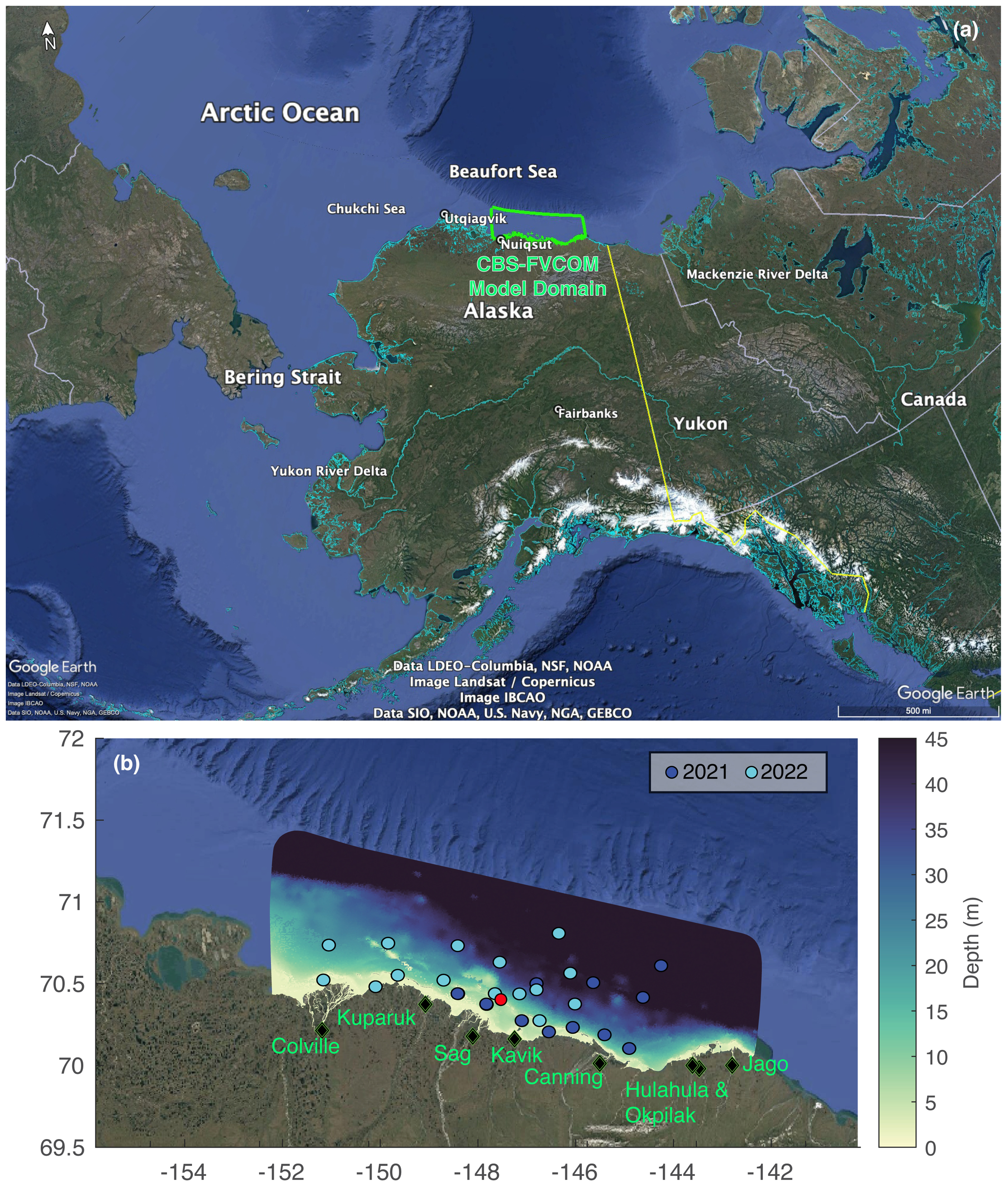
(a) The Northern Bering Sea and Pacific Arctic Ocean showing the main water bodies, large rivers, and the CBS-FVCOM domain outlined in green; (b) the model domain showing the rivers that were used to force the model with freshwater (black diamonds) and the station locations for the NASA/NRL 2021 and 2022 cruises used for model validation. The depth color scale was limited to 45 m, but the model depth extends to >1,000 m across the continental shelf. The red point indicates NOAA Tides and Currents station Prudhoe Bay, AK #9497645, which was used to compare sea surface height, water temperature, and wind velocity. CBS-FVCOM, Coastal Beaufort Sea Finite Volume Community Ocean Model.
The Colville River is the largest river draining the North Slope of AK, with a watershed area of 59,756 km2 (McClelland et al., 2014), of which 35,897 km2 is upstream of the United States Geologic Survey (USGS) gauge station at Umiat (69.3605° N, −152.1277° W). The Colville River has a mean annual discharge of 9.0 km3 at Umiat with the maximum daily discharge occurring on June 6, on average, based on measurements from 2003 to 2022. The Sag River is gauged at Pump Station 3 off the Dalton Highway (69.0158° N, −148.8178° W) with 4,792 km2 of the 12,580 km2 watershed upstream of the gauge station. The mean annual discharge for 2003–2022 was 1.62 km3, and the average day of maximum discharge at the gauge station was July 1. Unlike the Colville and Sag rivers, nearly the entire Kuparuk River watershed is upstream of the USGS gauge station near Deadhorse, AK (70.2817° N, −148.9597° W). For the 2003–2022 period (excluding 2011, for which data are unavailable), the Kuparuk River had a mean annual discharge of 1.57 km3, and, on average, the maximum daily discharge occurred on June 2. The Sag River is much steeper than the Colville and Kuparuk rivers, on average (McClelland et al., 2014). The final gauged river, the Hulahula River, drains into Kaktovik Lagoon in the far eastern portion of the model domain. The Hulahula watershed area is 1,779 km2 north of the USGS gauge station (69.7039° N, −144.1983° W), with a mean annual discharge of 0.51 km3, and the average day of maximum discharge was July 1 for 2003–2022. The other four rivers do not have continuous measurements of flow, and therefore, the river forcing at the model boundary was estimated using a combination of the other rivers, for simplicity. More details can be found in Section 3.4.
The coastal ocean along the North Slope of AK is relatively shallow and contains numerous lagoons bordered by islands. Detailed bathymetric data are lacking, but soundings taken during two research cruises were utilized to estimate the accuracy of the bathymetric data used for the model in the coastal areas. The ocean is covered with landfast ice and sea ice the majority of the year, with freeze-up historically occurring in October–November and ice persisting through May–June (Mahoney et al., 2014). The sea ice thaws from the east to the west, with the area around the Colville River delta typically maintaining sea ice the longest into the spring river freshet period (Mahoney et al., 2014). The major currents typically run west to east (Gao et al., 2011; Proshutinsky et al., 2005), and the large freshwater outflow of the Mackenzie River influences the hydrographic conditions in the Beaufort Sea, including the eastern portion of the model domain, especially during the spring freshet.
3 Methods
3.1 The Finite Volume Community Ocean Model for the coastal Beaufort Sea
The FVCOM (Chen et al., 2003) version 4.3 is a primitive equation three-dimensional hydrodynamic model that is based on an unstructured triangular grid geometric framework. The model is well-suited to represent areas with complex bathymetry and shorelines. The adaptive geometry of the unstructured mesh allows the spatial resolution of the model to stretch and bend to conform to geographic features such as islands and river deltas. Previously, multiple models have been tested and compared in the Arctic Ocean Model Intercomparison Project (AOMIP) (Proshutinsky et al., 2005), and papers describing various systematic aspects are held in a special collection in the Journal of Geophysical Research: Oceans (Proshutinsky and Kowalik, 2007). The FVCOM has been implemented in the Arctic at multiple resolutions (Chen et al., 2009; Chen et al., 2016; Gao et al., 2011) and recently in Elson Lagoon in the western coastal Arctic (Li et al., 2024), and the lower Yukon River and Northern Bering Sea (Clark and Mannino, 2022). The model solves for physical fluid properties in three dimensions with an internal and external mode split routine and calculates turbulence, temperature (T), salinity (S), horizontal (u and v) and vertical (w) velocity, and sea surface height (SSH). T, S, and SSH are calculated at each node connecting triangular elements, and velocity vector components are calculated at the element centers. The vertical domain is represented using vertically stretching sigma layers that make up a fixed proportion of the water column with the thickness of each layer dependent on the total water depth at each node.
The CBS-FVCOM has 230,064 triangular elements connected at 121,313 nodes, with 10 vertical layers that each make up 1/10th of the water column in an even proportion. The model was solved in hydrostatic mode with the time step generally 4 seconds external and 12 seconds internal, although time step reduction occurred when necessary to avoid numerical instability. Overall, runtime for the 1,734 model days would take ~6 wall clock days on 2,000 cores of the NASA Center for Climate Simulation supercomputer Discover. The bottom roughness length scale and roughness coefficient were spatially uniform at 0.001. The model was operated in the spherical coordinate system, and the turbulence closure was done using the MY 2.5 scheme (Mellor and Yamada, 1982). The horizontal mixing coefficient was 0.1, and the vertical diffusivity was set to 1 × 10⁻⁶. All model parameterizations can be found in the BLE_2018_2022_run.nml file in the repository.
The FVCOM has also been coupled with the Los Alamos sea ice model (CICE) (Hunke and Lipscomb, 2006) in the unstructured grid domain (FVCOM-UG-CICE), previously implemented across the Arctic to simulate interannual sea ice dynamics (Chen et al., 2016; Gao et al., 2011). The FVCOM has previously shown success in recreating historical sea ice observations and larger-scale currents (Chen et al., 2016; Gao et al., 2011) but was not configured until recently to represent parameterizations to account for landfast ice (Lin et al., 2022). The landfast ice formulations of Lemieux et al. (2015, 2016) were built into the FVCOM-UG-CICE and initially tested in the Great Lakes (Lin et al., 2022). Here, we incorporated the formulations specific for landfast ice to capture the different dynamics that drive landfast ice formation and persistence in Alaskan coastal waters. Ice formation and thaw influence the hydrodynamics in the ocean and therefore must be included to recreate ocean currents, temperature, and salinity even in ice-free months. The landfast ice and sea ice model setup, parameter tuning, validation, and analysis will be in the forthcoming manuscript, and initial results are promising.
3.2 Triangular grid construction
The unstructured triangular mesh in the FVCOM must meet specific quality requirements to prevent unstable and/or spurious model solutions. Multiple geospatial datasets were required to specify the shoreline and the bathymetry, which were both used to construct the unstructured mesh. The model bathymetry was defined from the 200-m-resolution International Bathymetric Chart of the Arctic Ocean (IBCAO) version 4.1 (Jakobsson et al., 2020). The model shoreline and islands were defined using the 1:250,000 Alaska Shoreline dataset (Gibbs and Richmond, 2017), a vector geospatial product that includes lower river reaches, river deltas, and coastal islands. The shoreline data file was cut to include only the North Slope region spanning our study area, and the various polygons were merged to create one continuous polygon in QGIS before being exported into the Aquaveo Surface Water Model Software (SMS version 13.1) for mesh generation.
The merged shoreline polygons and the IBCAO dataset were loaded into the SMS for triangular mesh construction. Both datasets were used in the polar stereographic projection (NSIDC EASE-Grid 2.0 North #6931) within the SMS to retain the most realistic spacing between locations within the model domain. The model grid spacing was set using the internal SMS data calculator function that calculates the wavelength of a gravity wave based on bathymetry. The grid spacing was set at the wavelength to the power of 1.25, which gave a range of 63 to 2,469 m of spacing between adjacent nodes, largely dependent on bathymetry. The model has a finer resolution in shallower regions (~50 m) (Figure 2a), stretches to resolve narrow channels and around islands, and coarsens toward the continental shelf, reaching a maximal resolution of ~2.5 km (Figure 2b). Each node was connected to a maximum of eight triangular elements. The bathymetric data were then linearly interpolated into the model in the SMS. The bathymetry was set to have a minimum value of 1.5 m because of uncertainty within the near-shore regions due to a general lack of observations in shallow waters in this region of the Arctic. However, sounding data obtained from a recent set of cruises in the area (Supplementary Material Figure S1) showed good agreement in the mid-shore regions, although there is a bias in the model in shallow areas, resulting in an underestimation of depth. The bathymetry was smoothed to avoid abrupt transitions between shallow areas moving away toward the continental shelf. The total depth range was 1.5 to 1,709 m. A new version of the model still being tested and to be included in a subsequent version has the recently published bathymetric dataset along the coast (Zimmermann et al., 2022), but the results presented here were carried out using the IBCAO data only. We have provided an additional file with statistical evaluation metrics using the new bathymetry showing minimal improvement in the predictions of SSH, T, and S in addition to statistical analyses using the same criteria as a separate file in the Supplementary Material.
Figure 2
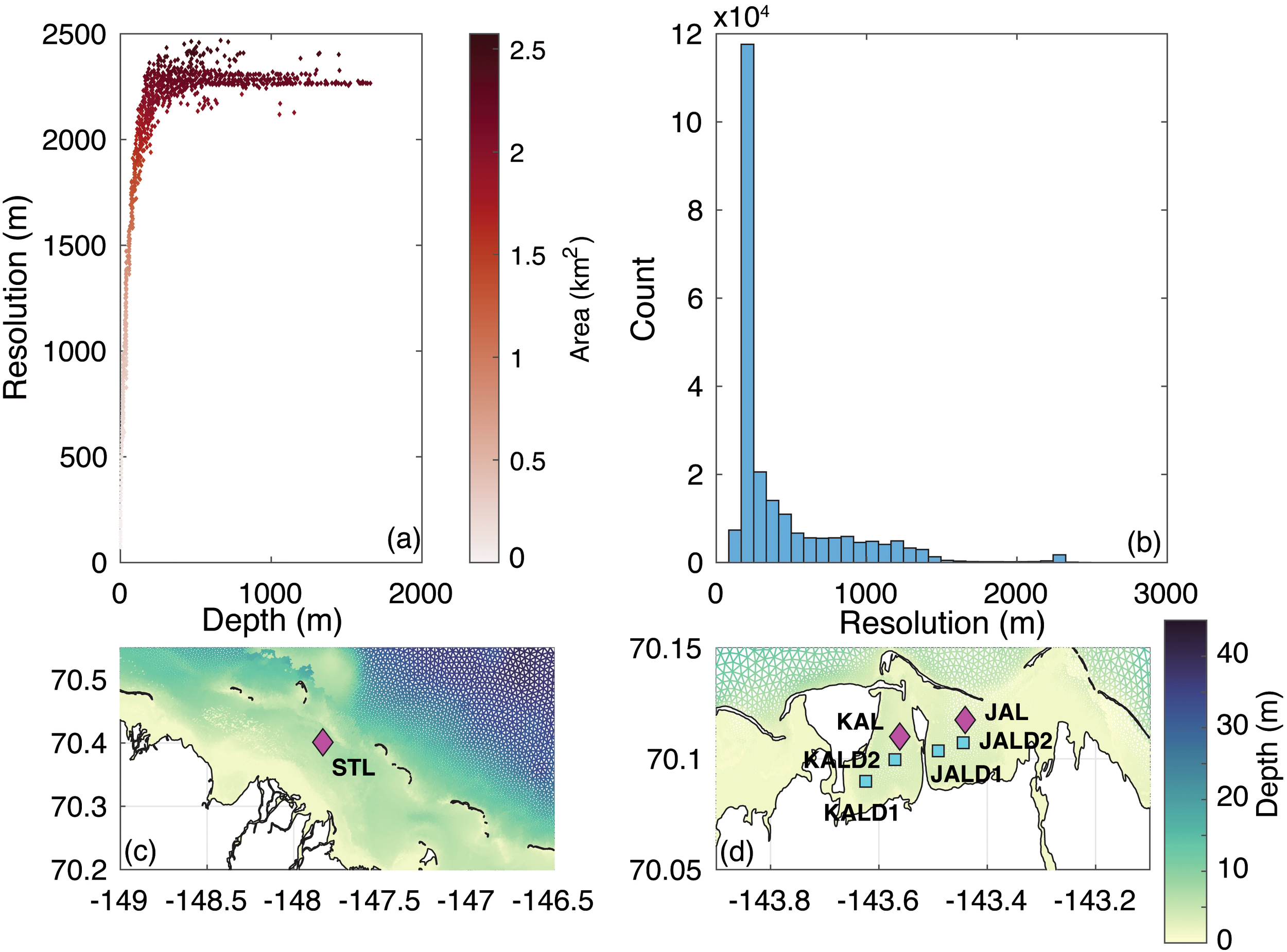
(a) Mean element grid spacing (distance of node to adjacent node) as a function of depth colored by the total area of the triangular element, (b) the distribution of the grid spacing, and zoomed-in plots of the mesh showing the BLE-LTER mooring stations for (c) Stefansson Sound near Prudhoe Bay and (d) Kaktovik and Jago Lagoon. The wiNAdiamonds are bottom-mounted moorings with velocity, depth, and temperature sensors, and the green squares are conductivity, temperature, and depth (CTD) sensors.
3.3 Surface weather forcing
The National Centers for Environmental Prediction (NCEP) North American Regional Reanalysis (NARR) (Mesinger et al., 2006) was used as the surface weather forcing. The weather data products are specified at each node or element across the model at a daily time step interpolated from the NARR grid to the closest model location using the nearest neighbor scheme. The weather forcing includes 10-m wind velocity vector components, downward longwave and shortwave radiation, surface pressure, precipitation and evaporation, relative and specific humidity, and cloud cover (Supplementary Material Figure S2). The COARE 26 Z algorithm (Fairall et al., 2003) is used within the FVCOM to calculate the sensible and latent heat fluxes. The CICE algorithm modifies the heat flux appropriately with the internal ice thermodynamics, although brine formation and ejection processes were not accounted for in this version of the CICE model used within the FVCOM 4.3. Wind velocity is converted to wind stress within the model, which imparts a force onto the ocean surface, driving surface currents within the model domain. Notably, an explicit wave model was not included in this version of the CBS-FVCOM. Cloud cover is utilized within CICE as a factor to account for ice albedo and longwave radiative balance within the ice formulations.
3.4 River forcing
Eight rivers were included in the model domain as freshwater flux and temperature forcings (Figure 1b). The river flow information was acquired from the USGS gauge station from January 1, 2018, to October 1, 2022, for the Colville, Kuparuk, Sag, and Hulahula rivers. River temperature was available only from the Kuparuk and Sag rivers and only during ice-free periods. The river discharge observation data were scaled to the total watershed area defined by HydroATLAS (Linke et al., 2019), including all areas up to the model coastline, using a simple proportional increase. The unmeasured rivers (Kavik, Canning, Okpilak, and Jago) were scaled by relative watershed area to the closest measured river, which was the Sag for the Kavik and Canning, and the Hulahula for the Okpilak and Jago. The time series of river discharge (Figure 3) show strong seasonality across each of the rivers over the model region. To account for the minimal flow of liquid water during the winter under the ice, river water temperature was set to be 0.1°C in the months from November to May. The temperatures for the Sag and Kuparuk rivers were then interpolated to a daily interval to match the daily mean river discharge dates. The average of the two monitored rivers was used as a proxy for the forcing on the other six rivers for which temperature measurements were not available (Figure 3b). All river inflow salinity was set to 0.0.
Figure 3
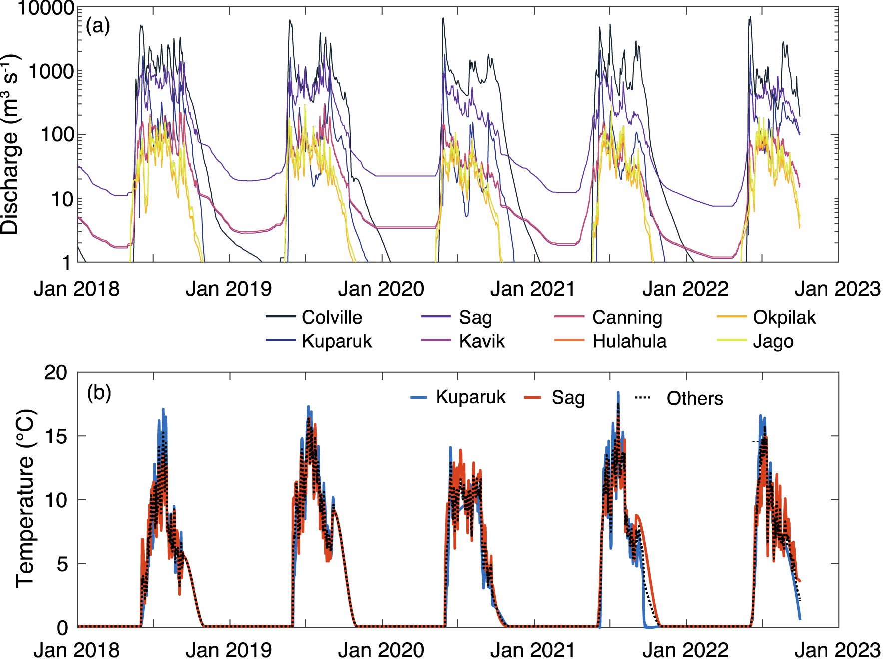
River forcing time series for the eight major rivers for (a) river discharge and (b) temperature. Temperature was only measured in the Kuparuk and Sagavanirktok rivers on a regular frequency, and therefore, the others were assigned as mean between the two. Note the log scale in panel (a).
3.5 Open boundary forcing
The open ocean boundary of the FVCOM requires oceanographic time series data to force the model. The needed data include depth-resolved T, S, and SSH, which drive the tidal forcing within the model domain. The Navy global HYCOM 1/12° Region 17 model predictions were utilized as the basis for the open boundary forcing (Chassignet et al., 2009; Metzger et al., 2014). T, S, and SSH were extracted at the HYCOM 8-h output frequency and directly interpolated in time and space to the model boundary using linear 3-D (T and S) and 2-D (SSH) methodologies using the MATLAB function griddatan.m. Where data were missing, a nearest neighbor approach was used, such as in shallow areas where the HYCOM model is not resolved. A map of the model study domain overlaid with the matching HYCOM Region 17 grid and the selected grid cells used for the boundary forcing can be found in Supplementary Material Figure S3. T and S are forced in the model at each boundary node and layer at a daily frequency.
The SSH forcing is on an hourly timescale to resolve the sub-daily tidal frequency. This required a combination of the HYCOM sub-tidal predictions and the OSU Tidal Prediction Software TPXO tidal predictions (Egbert and Erofeeva, 2002). The main tidal frequency components of SSH were calculated using TPXO, resolving the main components of the tidally driven SSH at each hour and each model boundary node specified in the TPXO input files. The HYCOM-estimated SSH was then extracted, low-frequency pass-filtered at a 36-h frequency to retain the sub-tidal variation in SSH that is not accounted for by the TPXO tidal prediction software, and then added back to the TPXO-predicted SSH. This combined HYCOM–TPXO product was used as the final boundary forcing for SSH, which drives the variations of SSH within the model. This importantly allows for capturing storm events that can drastically affect coastal SSH variation in this region that has a relatively low tidal range and could be important for future studies on erosion and inundation.
3.6 Model evaluation data and statistical analyses
3.6.1 Moorings and in situ measurements of velocity, SSH, temperature, and salinity
Multiple datasets were utilized to tune and evaluate the model throughout the development process and for the finalized simulation. Measurements collected during ship-based surveys in August 2021 and August 2022 as part of a NASA Ocean Biology and Biogeochemistry/Naval Research Laboratory collaborative field campaign were also utilized for model tuning and evaluation (blue-shaded dots in Figure 1b). These measurements included T and S measured from the YSI EXO2 sensor package that allowed a vertically distributed assessment of the model accuracy over a larger area. In 2021, only the surface and bottom (or the lowest reach of the instrument) were reported, while in 2022, vertical profiles were collected. The closest model point in time and space was identified for each cruise sampling station, and comparisons were made to assess the model’s accuracy. Finally, T and SSH measured at the NOAA Tides and Currents station in Prudhoe Bay (Station ID 9497645; 70.4117° N, −147.4683° W; red dot Figure 1b) were compared with the model estimates at the closest node within a lateral offset distance of 50 m. In addition, the NARR wind forcing was compared with measured wind velocity vector components at Prudhoe Bay for error analysis.
The BLE-LTER has time series data collected from moorings in Stefansson, Kaktovik, and Jago lagoons [Beaufort Lagoon Ecosystems Long Term Ecological Research (LTER), Core Program, 2018 to present] (Dunton and McClelland, 2021). Bottom-mounted moorings were deployed to measure current velocity, T, and SSH from August 2 to 9, 2018, to August 11 to 19, 2019, at one location in each lagoon (Figures 2c, d). Conductivity, temperature, and depth (CTD) sensors were also deployed at two locations each in Jago and Kaktovik lagoons from August 2–9, 2018, to August 11–19, 2019, which measured S and T, both of which were used for further model tuning and validation (Figure 2d). The mooring deployment details are in Table 1, and information on the specific instrumentation, mooring setup, and data processing can be found in the associated metadata from the BLE-LTER data hub (https://ble.lternet.edu/catalog). Mooring data and modeled data were averaged over each day and matched in time and space for statistical comparisons. The closest model node (for T, S, and SSH) and element center (for u and v velocity components) to the observation location were used. Target diagrams utilized the data aggregated by month to assess model performance across the year rather than in total.
Table 1
| Current tilt meters | ||||||||
|---|---|---|---|---|---|---|---|---|
| Station | Location | Period (DD/MM/YYYY) | SSH ± σ (m) | N | u ± σ (cm s−1) | v ± σ (cm s−1) | T ± σ (°C) | |
| JAL | 70.1667° −143.4400° |
Aug 9, 2018 Aug 11, 2019 |
2.94 ± 0.18 | 8,816 | 2.69 ± 5.34 | −2.20 ± 6.18 | −0.28 ± 2.60 | |
| KAL | 70.1108° −143.5608° |
Aug 9, 2018 Aug 11, 2019 |
3.10 ± 0.18 | 8,817 | 0.79 ± 2.31 | −0.03 ± 1.76 | 0.35 ± 3.46 | |
| STL | 70.4021° −147.8367° |
Aug 2, 2018 Aug 19, 2019 |
6.85 ± 0.20 | 9,189 | 2.48 ± 6.42 | −0.27 ± 5.17 | −1.03 ± 1.68 | |
| Conductivity, temperature, and depth sensors | ||||||||
| Station | Location | Period | SSH ± σ (m) | N | T ± σ (°C) | S ± σ | ||
| JALD1 | 70.1041 −143.4892 |
Aug 8, 2018 Aug 11, 2019 |
NA | 8,815 | −0.13 ± 2.69 | 30.92 ± 7.23 | ||
| JALD2 | 70.1068 −143.4435 |
Aug 8, 2018 Aug 11, 2019 |
3.35 ± 0.18 | 8,816 | −0.24 ± 2.49 | 35.38 ± 6.80 | ||
| KALD1 | 70.0890 −143.6233 |
Aug 7, 2018 Aug 10, 2019 |
NA | 8,839 | 0.20 ± 3.56 | 29.79 ± 10.72 | ||
| KALD2 | 70.1009 −143.5709 |
Aug 7, 2018 Aug 10, 2019 |
2.87 ± 0.38 | 8,839 | 0.18 ± 3.53 | 33.18 ± 7.57 | ||
Mean and standard deviation (σ) of the u and v velocity vector components, temperature (T), and salinity (S) for the Beaufort Lagoon Ecosystems LTER mooring data collected in the lagoons in 2018–2019 at the locations in Figure 2.
N is the number of observations (hourly) over the observation period.
LTER, Long Term Ecological Research; SSH, sea surface height.
3.6.2 Statistical analysis
All model-observation comparisons were assessed using the Nash–Sutcliffe model efficiency (MEF; Equation 1) (Nash and Sutcliffe, 1970; Stow et al., 2009), the correlation coefficient (R2) as the square of Pearson’s correlation coefficient (r; Equation 2) (Stow et al., 2009), the median symmetric accuracy (ζ; Equation 3) (Morley et al., 2018; Smith et al., 2021), and the symmetric signed percentage bias (SSPB; Equation 4) (Morley et al., 2018; Smith et al., 2021). MEF is a measurement of the model’s ability to represent the modeled variable, y, relative to the observational variable, x, compared to the mean, ; an MEF of 0 indicates that the model is no better than the mean at representing the data, while a value of 1 indicates a perfect fit. ζ is the percentage of the exponentially transformed median (M) of the absolute value of the natural log (ln) of the ratio of the predictions (y) to the observations (x) (Equation 3). ζ mitigates problems related to the penalization of over- and under-estimation and the effects of outliers skewing the interpretability while necessarily operating across multiple orders of magnitude (Morley et al., 2018). SSPB (Equation 4) further utilizes the concept of ζ and assigns a sign, sn, by utilizing the sign (+1 or −1) of the median absolute log ratio (the exponent in Equation 3). SSPB and ζ are useful metrics to assess model-data comparisons across multiple orders or magnitudes.
The downside to utilizing statistical analyses that operate in the log space is the difficulty with negative values and zeros, which often occur in oceanographic and aquatic variables such as T, S, SSH, and velocity vector components. Therefore, variables where negative and zero values are possible (except ice cover) were transformed by subtracting the minimum value (mostly negative or zero) and adding 1 × 10⁻⁸– to avoid zeros. This allows for the use of log-based statistics for these variables without altering the magnitude and variance within the data. R2, MEF, and root mean square difference (RMSD; Equation 5) utilized the un-transformed values before scaling.
Target diagrams were also produced to summarily display the model-observation matchups for ice, velocity, and other variables (Jolliff et al., 2009). These diagrams place the modeled-observation comparisons into RMSD space, utilizing the unbiased RMSD (uRMSD) (Equation 6) multiplied by the sign, sn, of the difference in standard deviation, σ, and bias (Equation 7). The distance from each point is thus equal to the total RMSD. All other variables used uRMSD in non-normalized native units.
4 Results: model evaluation and analysis
4.1 Comparison with in situ hydrodynamic data
4.1.1 NOAA Tides and Currents SSH and water temperature
The NOAA Tides and Currents observation station in Prudhoe Bay allowed for a direct comparison of the measured T and SSH (Figure 4). Overall, the model accurately estimated the seasonal progression and interannual variability of the daily average T (Figure 4a). The model did not capture some of the variability observed in the spring and summer months, but the drawdown from summer into fall was well recreated for 2019, 2020, and 2021. The very low wintertime T was not captured for any of the four years for which data were available, with the measured T nearing −1.9°C in the winter months, while the modeled T never got below −1.75°C. This is exhibited by the positive SSPB and ζ, although MEF and R2 were 0.51 and 0.48, respectively, indicating that the temporal variances were well represented (Table 2). The lack of the ability to reach very low temperatures in the winter is a challenging aspect of this system, as the minimum modeled temperature is based on the freezing temperature of water at a given salinity and thus also depends on the model’s ability to accurately predict salinity. This will be discussed further in Section 4.1.3.
Figure 4
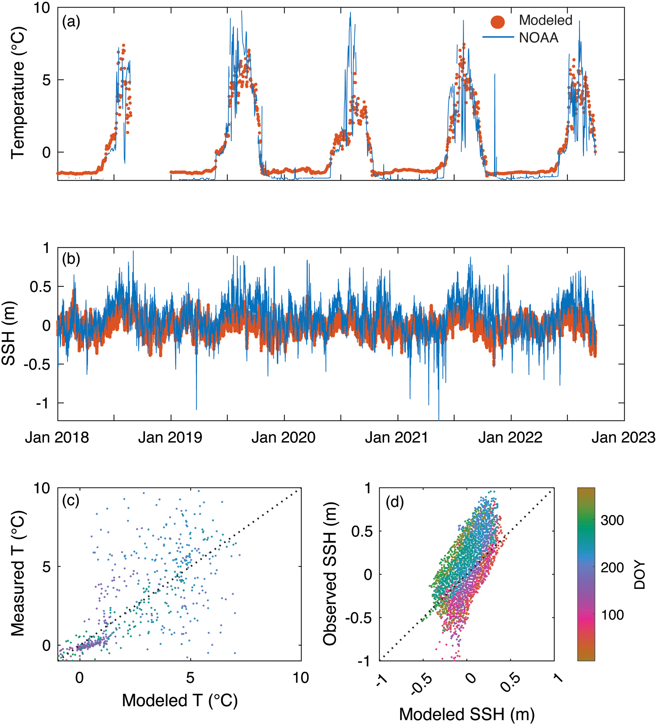
Model-data comparison of NOAA Tides and Currents station 9497645 of daily average (a) temperature and (b) matched hourly velocity, with panels (c, d) showing the same data. DOY stands for the day of the year.
Table 2
| n matches | RMSD (salinity or °C) | MEF | R2 | ζ (%) | SSPB (%) | |
|---|---|---|---|---|---|---|
| Daily T | 1,604 | 1.82 | 0.51 | 0.48 | 170.9 | 116.5 |
| Hourly SSH | 41,592 | 0.19 | 0.18 | 0.44 | 11.15 | −8.64 |
| Filtered SSHa | 41,592 | 0.19 | 0.13 | 0.42 | 18.5 | −14.2 |
| Diurnal tidalb component | 41,592 | 0.04 | 0.70 | 0.71 | 5.67 | −0.13 |
Comparison of daily averaged model output of sea surface height (SSH) and water temperature (mean of upper three layers of the model) with NOAA Tides and Currents station 9497645 at −148.5317° W and 70.4117° E.
RMSD, root mean square difference; MEF, model efficiency; SSH, sea surface height.
Filtered SSH uses a moving box car filter with a cutoff frequency of 36 hours to remove the diurnal tidal signal.
Diurnal tidal component is the filtered signal minus the actual SSH, thus removing the non-diurnal tidal component due to other factors.
The hourly SSH was well recreated in the model (Figure 4b), including inter-tidal and inter-seasonal variations in SSH (Table 2). SSH residuals (errors) were generally evenly distributed (Supplementary Material Figure S5), so the SSPB and ζ were relatively low, although there was a slight negative bias in the sub-tidal and diurnal tidal components (Table 2). Removing the tidal signal using a low-frequency pass filter of 36 h led to an MEF of 0.70 and R2 of 0.70, which also indicated somewhat strong predictive capability beyond the semi-diurnal tidal frequency. When analyzed monthly (Supplementary Material Table S1), the MEF declined in warmer months, although R2 increased, in addition to subsequent increases in RMSD. This seasonal bias suggests that predictive capacity within the model for estimating SSH declines as the ice recedes. In general, the tidal range is quite small in this area, and the influence of ice on dampening surface-driven variation in the winter likely contributed to the lower errors in cold months and larger errors in ice-free months. This phenomenon warrants more investigation on trying to capture SSH dynamics in these shallow coastal waters, which may include changing parameterizations on the bottom drag coefficient within the FVCOM. Across all five years, the high R2 and MEF indicate that the temporal variance was captured quite well within the FVCOM despite missing some of the extrema in SSH and some of the high SSH in the summer.
4.1.2 NASA/NRL 2021 and 2022 cruises
The cruise data collected in 2021 and 2022 provided a spatial comparison across the nearshore regions, which is important for validating the spatial variability in hydrodynamics within the modeling system. The measurements in 2021 included the surface (matched to the top layer of the model) and bottom measurements of T and S, while full vertical profiles recorded every 1 second and binned in 0.5 m were acquired in 2022. Overall, S was better predicted by the model in both years, relative to T, with S having low ζ and SSBP and being positively correlated (R2 = 0.58 and R2 = 0.29 in 2021 and 2022, respectively; Table 3) with the observations (Figures 5a–d). In 2021, the modeled T was generally underestimated relative to the observations, while in 2022, there was a depth-varying bias, with surface T underestimated and bottom T overestimated (Figures 5b, d). This indicates that the modeled water column, relative to observations, is less thermally stratified even though the salinity comparison across depth has little bias.
Table 3
| Salinity | Temperature | |||
|---|---|---|---|---|
| Metric | 2021 | 2022 | 2021 | 2022 |
| RMSD | 4.35 | 4.08 | 2.31 | 1.90 |
| MEFa | 0.35 | −0.02 | −1.01 | −0.11 |
| R2b | 0.58 | 0.29 | 0.14 | 0.02 |
| ζ (%)c | 8.33 | 12.8 | 45.2 | −08.2 |
| SSPBd % | 6.28 | 2.34 | −45.2 | −108.2 |
Comparison statistics of the model predicted temperature and salinity with the NASA/Naval Research Laboratory sponsored cruise data collected in 2021 and 2022 on the R/V Ukpik.
RMSD, root mean square difference.
Nash–Sutcliffe model efficiency (MEF) with a value greater than zero indicates that the model is better at representing the data relative to the mean (Nash and Sutcliffe, 1970; Stow et al., 2009).
Correlation coefficient (Stow et al., 2009).
Median symmetric accuracy (Morley et al., 2018).
Symmetric signed (Morley et al., 2018).
Figure 5
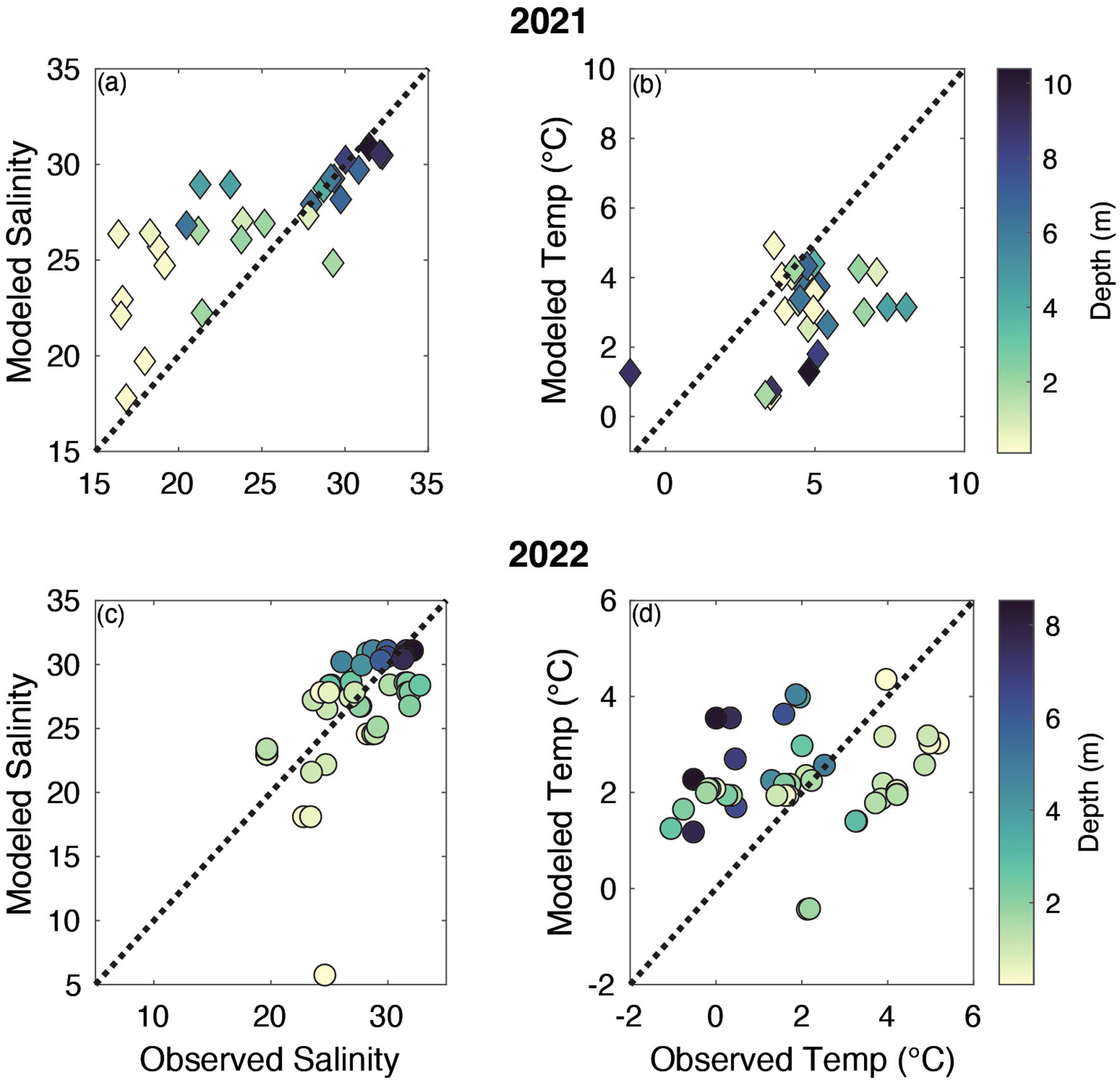
Modeled vs. observed (a) salinity and (b) temperature in 2021 and (c) salinity and (d) temperature in 2022 from the OBB research cruises.
In past implementations of the FVCOM where sea ice was not being predicted, T was generally well modeled (Clark and Mannino, 2022) and S was usually more difficult to predict, especially in nearshore river-influenced/stratified systems. This indicates that the sea ice thermodynamics and seasonal cycle provide some degree of regulation of T into the summer and that small deviations in sea ice predictions and sea ice cover can have large effects on the summertime water T. The sea ice implementation in the model did not account for nuanced ice thermodynamics that may be important in these shallow coastal areas of the Arctic. These include mechanistic brine dynamics, melt pond formation, and a more sophisticated treatment of snow cover and solar irradiance penetration that heats the water column such as in the newest version of CICE (CICE 6.6.0 Hunke et al., 2024). There are now formulations for including some aspects of these processes within the CICE framework, and ongoing work continues to update the model to include these processes more mechanistically. In addition, the biological aspects of the water column may also regulate the finer-scale aspects of water column heating in the spring. These include ice algae formation and solar irradiance absorption and the absorption of ultraviolet–visible light by terrestrially derived and strongly humic colored dissolved organic matter (CDOM) (Hill, 2008) as well as CDOM ejected with brine (Hill and Zimmerman, 2016). CDOM absorbs UV and visible light energy in the upper ocean, leading to thermal energy retention and driving up to 48% of the sea ice melt in the Chukchi Sea (Hill, 2008). The potential increase in coastal CDOM as river flows increase (Clark et al., 2023) can lead to further ice loss and heating due to river inflow effects as a positive climate feedback. However, to include these biochemical feedbacks in the model as currently constructed would require two-way coupling between the biogeochemical model (Clark et al., 2022) and the CBS-FVCOM, which is currently run offline from the hydrodynamic model.
4.1.3 Lagoon temperature, salinity, and velocity
The bottom-mounted moorings in Stefansson (STL; Figure 2c) and Jago and Kaktovik lagoons (JAL and KAL; Figure 2d) and the bottom-mounted temperature and salinity sensors in Jago and Kaktovik lagoons (JALD1, JALD2, KALD1, and KALD2; Figure 2d) allowed comparisons to assess the model’s ability to capture temporal trends of S in these shallow lagoon environments over an entire year. Model-data comparison statistics are available in the Supplementary Material file Table2.xls, and MEF and R2 respectively varied from 0.82 and 0.86 (JALD2) to 0.91 and 0.92 (KALD1). Seasonal trends in T were captured quite well by the model, with the drawdown occurring in September/October, followed by periods of sub-zero T in the winter and subsequent thaw and T increase in June/July (Figure 6). There were strong intra-seasonal variations in Stefansson Sound (Figure 6a) in the fall of 2018 and the spring of 2019 that were largely not captured by the CBS-FVCOM, and the modeled winter T at Stefansson Sound was warmer than observations. Jago Lagoon and Kaktovik Lagoon, however, both showed a better comparison across all seasons, with inter-seasonal and short-term variations captured quite well (Figures 6b, c). Statistical analyses indicated good predictive capability for all three locations (Stefansson MEF = 0.50, Kaktovik MEF = 0.94, and Jago MEF = 0.78).
Figure 6
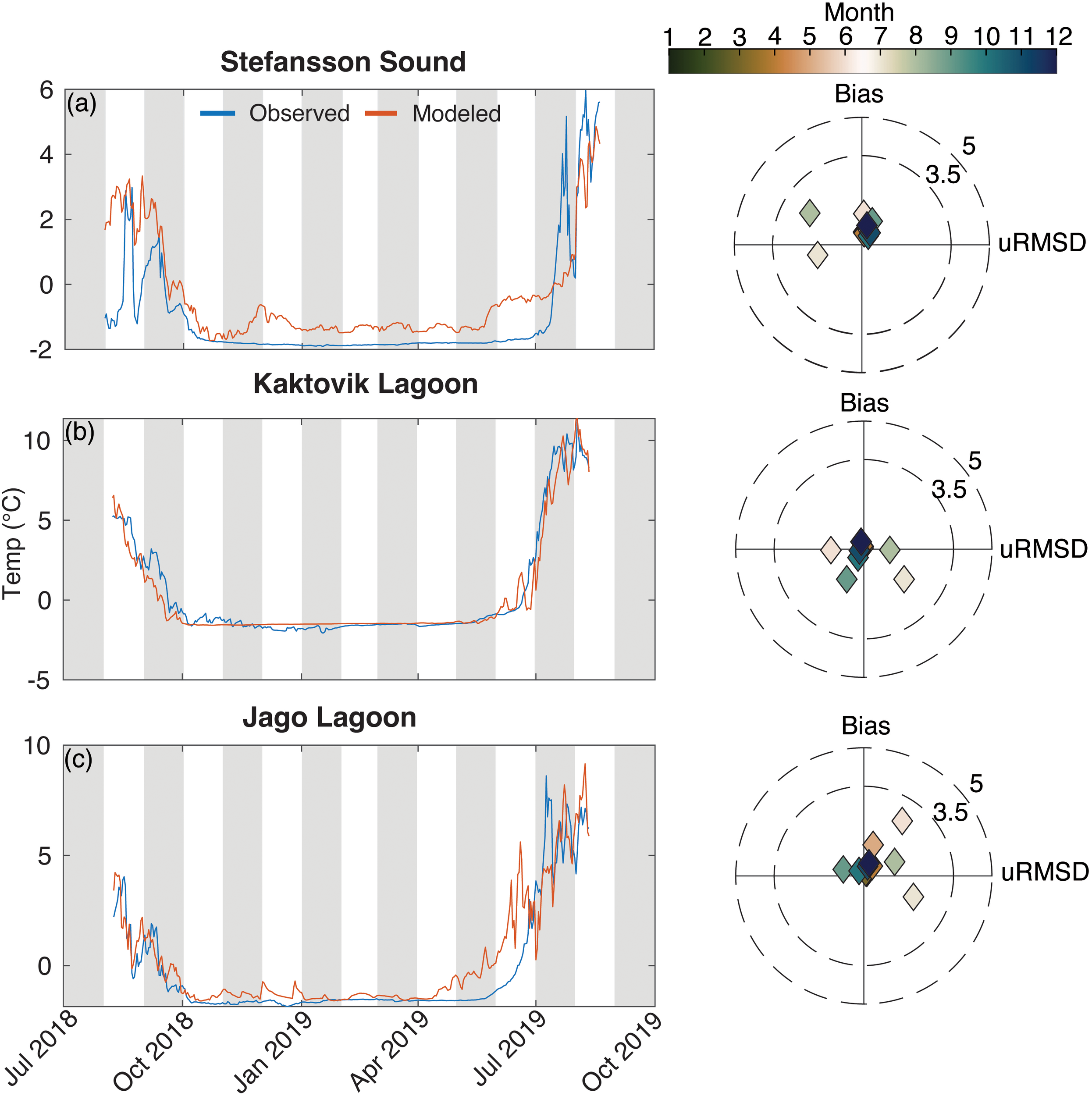
Comparison of daily averaged model predicted temperature vs. Beaufort Lagoon Ecosystems Long Term Ecological Research for (a) Stefansson Lagoon, (b) Jago Lagoon, and (c) Kaktovik Lagoon. The associated target diagrams are in the same units. Target diagrams indicate the model’s bias (y-axis) as a function of its variability (x-axis) relative to the observations. A bullseye indicates that the model has no bias and has the same variance as the observations.
The model-predicted SSH in the lagoons showed very little bias across seasons, with the daily averaged modeled SSH capturing the patterns of variation quite well for 2018–2019 (Figure 7). The model SSH was relatively dampened compared to observations (similar to Prudhoe Bay), with uRMSD substantially less for model predictions relative to the observations (Figure 7). High water events in September 2018, February–March 2019, and April–May 2019 occurred at all three locations and were represented in the model. Generally, the statistics show good agreement between the model and observations at these stations, and in combination with the SSH comparisons from Prudhoe Bay (Figures 4b, d), we conclude the model had sufficient skill at capturing SSH.
Figure 7
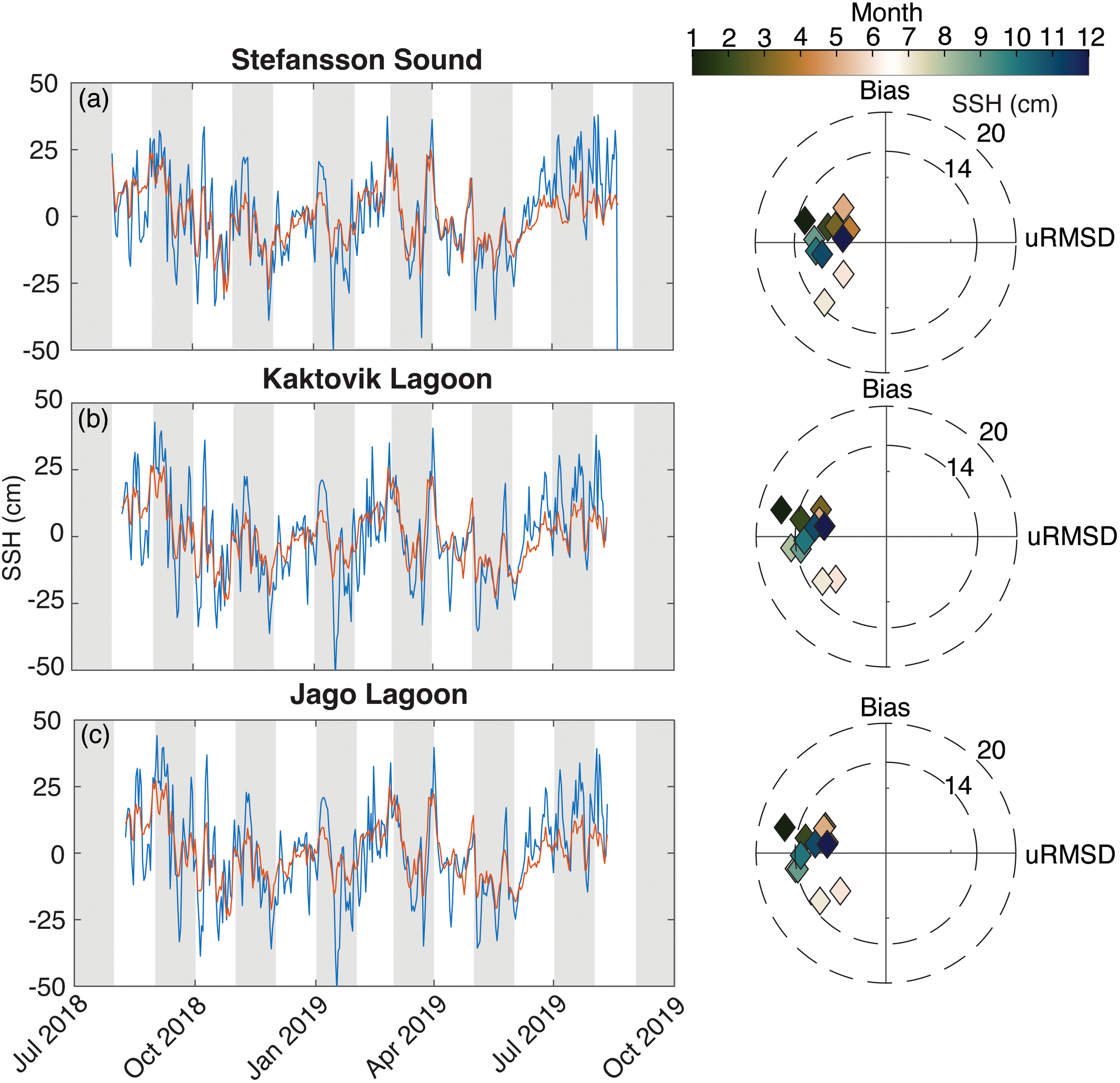
Comparison of daily averaged model predicted sea surface height (SSH) vs. Beaufort Lagoon Ecosystems Long Term Ecological Research for (a) Stefansson Sound, (b) Jago Lagoon, and (c) Kaktovik Lagoon. The associated target diagrams are in the same units. Target diagrams indicate the model’s bias (y-axis) as a function of its variability (x-axis) relative to the observations. A bullseye indicates that the model has no bias and has the same variance as the observations.
Daily mean west-to-east (u; Figure 8) and south-to-north (v; Figure 9) current velocity showed less agreement among the model and the mooring measurements. MEF for both vector components at all three stations were less than 0, indicating that for a given day, the mean value would give a better estimate for velocity than the model predictions. However, the model fidelity for predicting velocity varied seasonally and between years, as indicated by the insets for the ice-free periods (Figures 8, 9c, d, g, h, k, l). There was a pronounced seasonally varying bias in the u velocity in Jago and Kaktovik lagoons (Figures 8e, f, i, j), with the model-predicted wintertime u less the consistent eastward flow. This is when the lagoons are covered in ice and there is very little exchange and surface energy momentum transfer to drive currents. Jago Lagoon exhibited this bias across all seasons (Figure 8f), as indicated by negative values on the y-axis of the target diagram. There was little bias in the Stefansson Sound u velocity in the winter (Figure 8b), although there was an obvious lack of ability to estimate u velocity in Stefansson Sound in the summer/fall of 2018 (Figure 8c). This contrasts with good model performance in the spring/summer of 2019. This qualitative comparison is reinforced by the evaluation statistics: the Stefansson Sound summer/fall u velocity in 2018 had poor predictive capability (MEF = −2.18; R2 = −0.12), while in 2019, the model’s predictive capability improved dramatically (MEF = 0.11; R2 = 0.29). The opposite pattern held for Jago and Kaktovik lagoons, with the summer/fall of 2018 both having a better model-data comparison than 2019 and the overall time series. In addition, model performance for v velocity was worse for all three lagoons in the spring, summer, and fall.
Figure 8
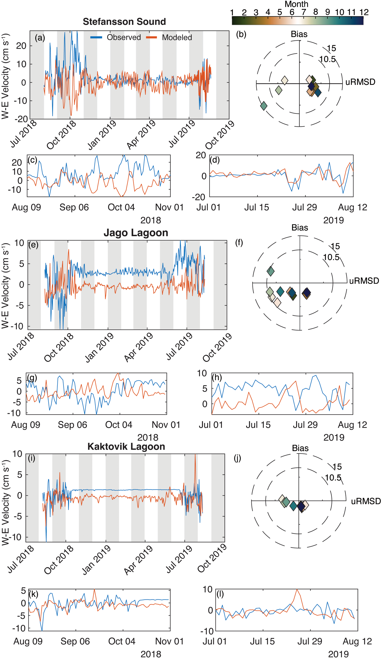
Comparison of daily averaged model predicted west to east (W–E) velocity vs. Beaufort Lagoon Ecosystems Long Term Ecological Research for (a–d) Stefansson Lagoon, (e–h) Jago Lagoon, and (i–l) Kaktovik Lagoon. The associated target diagrams are in the same units, and the insets show the velocity in the ice-free periods. Target diagrams indicate the model’s bias (y-axis) as a function of its variability (x-axis) relative to the observations. A bullseye indicates that the model has no bias and has the same variance as the observations.
Figure 9
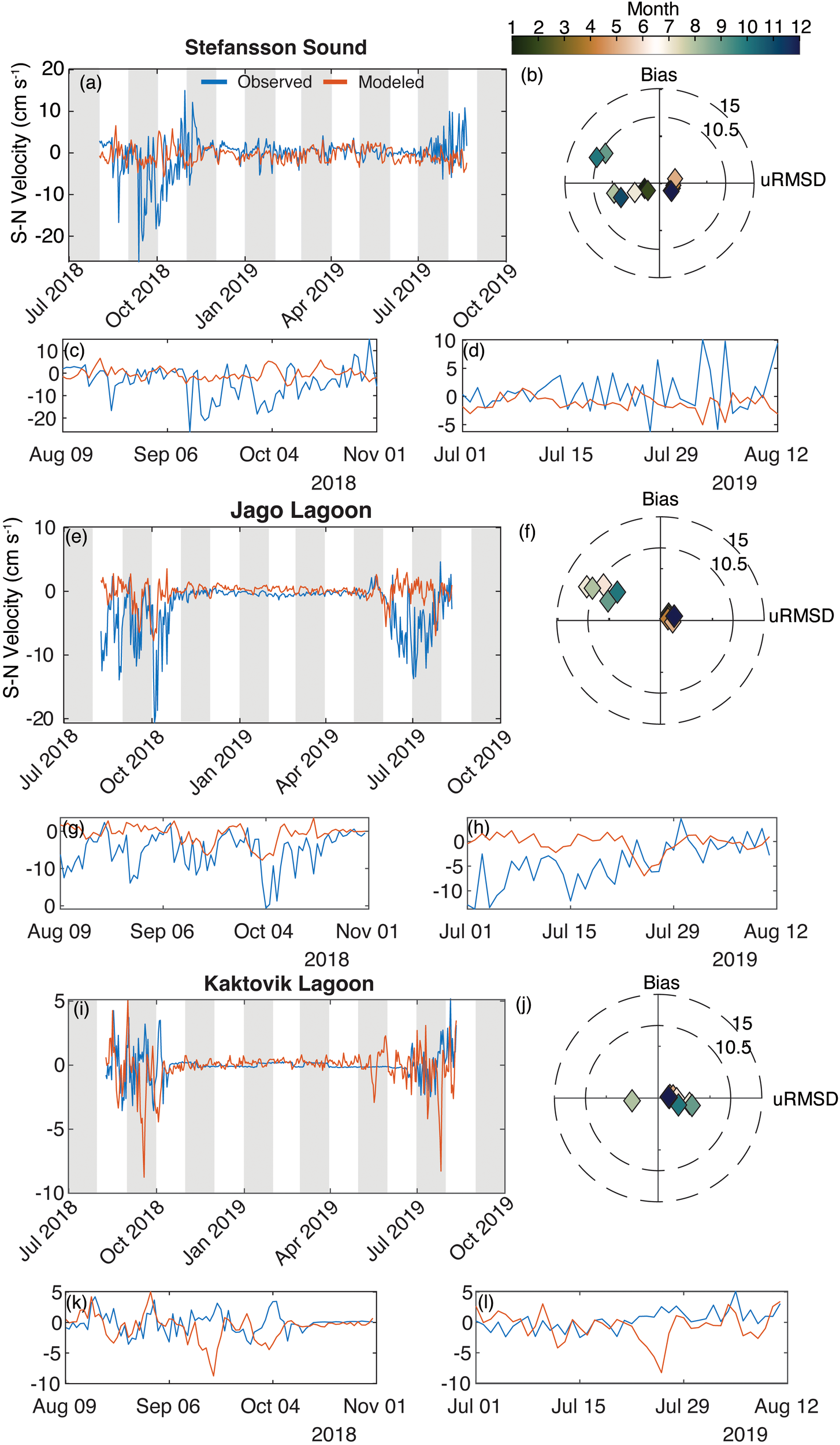
Comparison of daily averaged model predicted south to north (S–N) velocity vs. Beaufort Lagoon Ecosystems Long Term Ecological Research for (a–d) Stefansson Lagoon, (e–h) Jago Lagoon, and (i–l) Kaktovik Lagoon. The associated target diagrams are in the same units, and the insets show the velocity in the ice-free periods. Target diagrams indicate the model’s bias (y-axis) as a function of its variability (x-axis) relative to the observations. A bullseye indicates that the model has no bias and has the same variance as the observations.
The measurements of T and S in Kaktovik and Jago lagoons (green squares in Figure 2d) showed high overall skill at capturing the seasonal variation in T while missing some of the short-term intra-seasonal variation, like the other lagoon mooring measurements (Figures 10a–d). S was also generally captured well in the ice-free months (August–October 2018 and June–August 2019), although S at KALD1 in 2019 was poorly represented, as the model missed the near-zero values that occurred in the spring (Figure 10c). Modeled S in the winter was underestimated at each lagoon during the ice-covered months, unable to represent the slow accumulation of hypersaline water until the spring thaw in May–June 2019. The modeled S remained flat through the fall and winter, near 30 for each lagoon, while the observations showed a gradual increase in S over time. This upper limit of modeled salinity is based on a simple linear regression of the freezing temperature of seawater in the UG-CICE model. More discussion will occur in Section 5.
Figure 10
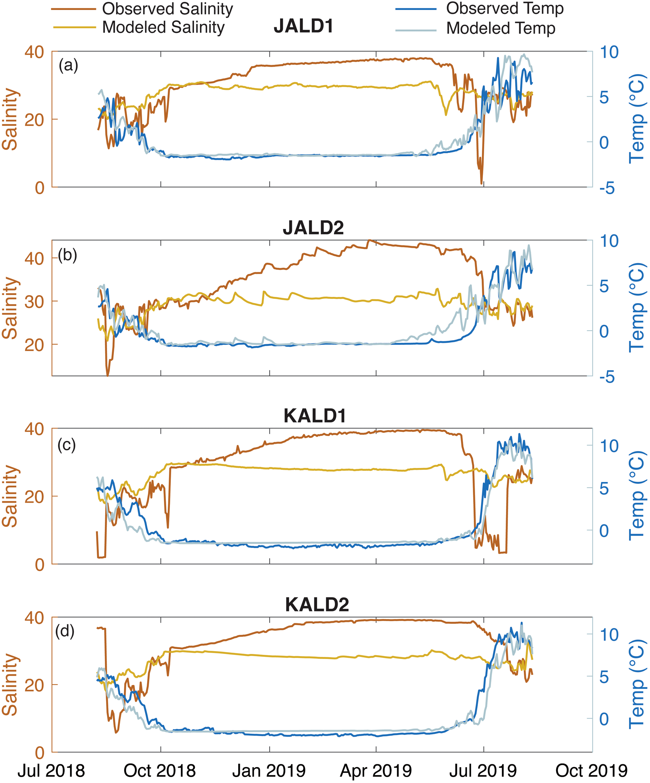
(a–d) Time series of model predictions and observations of water temperature and salinity from bottom moorings in Jago and Kaktovik lagoons with the titles corresponding to the station locations in Figure 2d.
4.1.4 Wind velocity, sea surface height, and current velocity error analysis
The complex patterns of observed velocity across the lagoons warranted further investigation. NARR forcing for the grid cell over Prudhoe Bay was notably dampened compared to the NOAA observations (Figures 11a–d). The values of mean ± standard deviation for the modeled magnitudes of the u and v wind forcing components (u = 3.23 ± 2.43 m s−1 and v = 1.43 ± 1.01 m s−1) were much lower than those for the measured u and v wind components (u = 5.74 ± 4.12 m s−1 and v = 1.72 ± 1.35 m s−1). Overall, u was much stronger than the v component, indicative of the typical easterly wind regime over the region. The errors were generally normally distributed, with the mean residuals for u and v near 0 (u = 0.83 m s−1 and v = −0.64 m s−1) (Figures 11c, d). The errors in wind forcing and the connection between ocean currents afforded exploration of how wind forcing uncertainty can affect the hydrodynamic (SSH and current velocity) performance of the model.
Figure 11
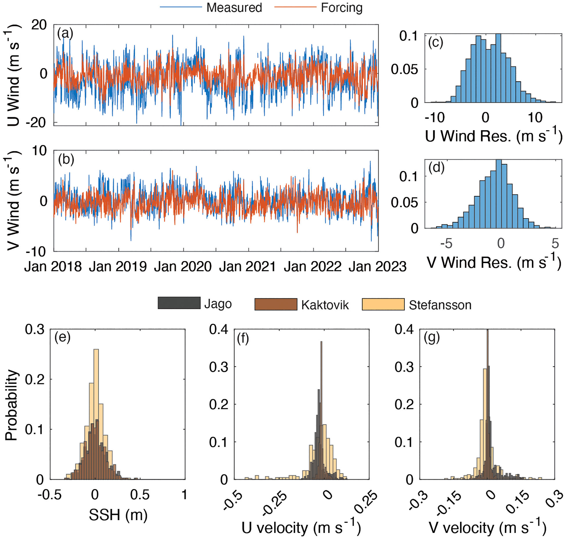
Time series of wind (a)u and (b)v North American Regional Reanalysis Forcing and observations at NOAA Tides and Currents station Prudhoe Bay, the residuals of the forcing minus observations (c, d) and the residuals of the modeled minus observed (e) sea surface height (SSH), (f) west–east (u) current velocity, and (g) south–north (v) current velocity at the three bottom-mounted moorings in the lagoons.
There was a clear offset in the wintertime west–east bottom current velocity in Jago and Kaktovik lagoons (Figures 8e, i), but the relationship between the wind velocity, SSH, and bottom current velocity in the ice-free months was less clear. Using the MATLAB function xcov, the cross-covariance analysis of wind forcing velocity components, SSH, and current velocity components was conducted for each time series from August to November 2018 to exclude ice-covered periods. Cross-covariance measures the covariance between two stationary time series at varying time lags (± 10 days in this study) to assess the temporal variation between two time series. Time series were normalized to the range of 0–1 to remove the effects of the sign convention. In addition, modeled minus observed wind forcing residuals were compared with SSH residuals and current velocity component residuals for each lagoon to quantify how potential error in the surface wind forcing could propagate into the hydrodynamics.
u wind forcing and residuals were strongly related to SSH in each lagoon (coefficient of covariance, C = 0.62–0.70) (Figures 12a, b). v wind forcing residuals were strongly related to the SSH residuals (C = −0.41 to −0.60), indicating that underpredictions in v wind forcing magnitude (less extrema) drove larger errors in SSH. v wind velocity was generally lower in magnitude with smaller residuals relative to u wind velocity (Figures 11c, d), but the strong anti-covariance between v wind residuals and SSH residuals indicates that SSH is more sensitive to variance in v wind relative to u wind. Strong northward (positive) v winds drove water offshore and out of the lagoons, leading to a decrease in SSH, while strong southward (negative) v winds drove water onshore, increasing SSH. The relatively dampened v wind forcing magnitude thus drove the underprediction of SSH magnitude in the opposite direction of the forcing. The opposite pattern holds for u winds. In the absence of other forcing, eastward (positive u) wind pushes water onshore, while westward (negative u) wind pushes water offshore. The strong positive covariance in forcing magnitude and SSH indicates that overall wind drives much of the sub-tidal variance in SSH in all three sites.
Figure 12
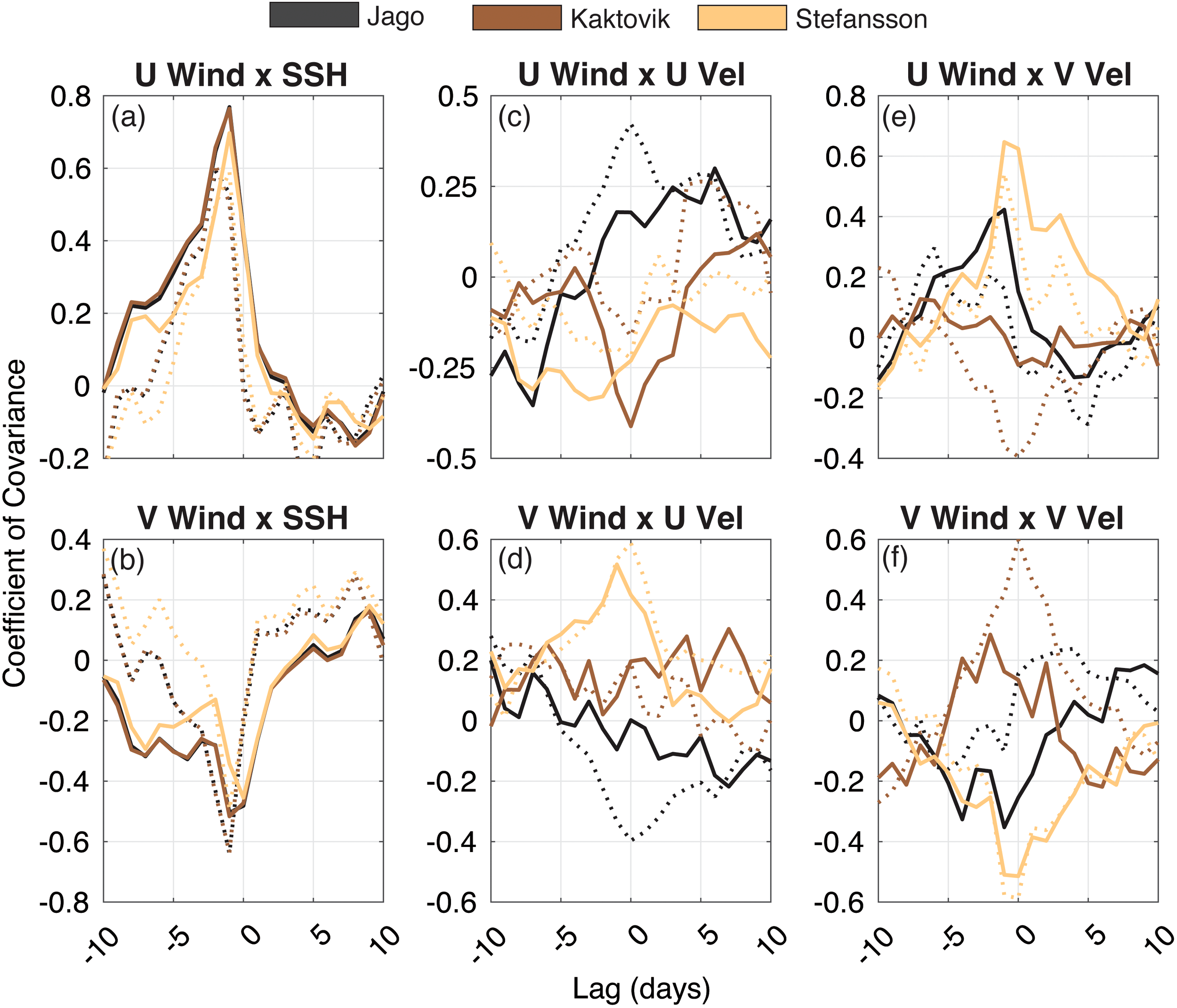
Cross-covariance of observed wind velocity vector components at Prudhoe Bay and of observed (a, b) sea surface height (SSH), (c, d)u current velocity, and (e, f)v current velocity at the three moorings. Solid lines are for the magnitude of the observations, and the dashed lines represent the cross-covariance of the residuals of the wind (forcing minus observed) and the bottom current velocity (modeled minus observed).
Wind velocity had varying effects on the bottom current velocity and residuals, with cross-covariance between wind and bottom current velocity components exhibiting inconsistent patterns across locations, relative to SSH. The strongest covariance occurred between wind and current velocity in Stefansson Sound, with Jago and Kaktovik lagoons exhibiting inconsistent and weak covariance with wind overall. Jago and Kaktovik lagoons are shallow and enclosed, and the fetch of the wind and exposure to the open ocean is much less than where the Stefansson Sound mooring is located. The Stefansson Sound u wind did not cross-covary with u current velocity magnitude or residuals (Figure 12c), but u current velocity moderately covaried with v wind (Figure 12d). The Stefansson Sound v current velocity and residuals were more closely coupled to wind (both u and v; Figures 12e, f) and followed the same direction of cross-covariance as SSH.
In mid-September 2018, there were two pronounced storm events when the observed bottom u and v current velocity increased for a sustained period, coinciding with strong northeastward winds blowing offshore toward the Beaufort Sea. Prior to September 12, u wind and u current velocity positively covaried, and v wind was relatively weak. Beyond September 12, they were decoupled, with the u current velocity opposite of the u wind (Figure 8a), and the v current velocity was consistently negative, indicating a southeastward bottom flow—opposite of the northward winds. This is indicative of an upwelling pattern that would be driven by the offshore and downcoast (eastward) wind velocity, a priori. However, the model current velocity was not sensitive enough during these wind events to recreate this two-layer flow, possibly because the model wind forcing was much lower in magnitude. Without observations of water column profile velocity, upwelling cannot be confirmed. However, these limited results suggest that northward winds can drive upwelling favorable conditions that may lead to strong shoreward bottom currents. This has implications for sediment redistribution, ice movement, and coastal bluff erosion, among other oceanographic processes. However, without distributed observations of surface wind and water column water velocity (surface and bottom, at minimum), the relationship of wind to ocean currents in these topographically complex systems is difficult to fully quantify.
The Stefansson Sound mooring was more exposed to the open ocean and therefore more influenced by larger-scale current dynamics and oceanographic processes. Comparison to the closest grid point from the NAVY 1/12° HYCOM model indicates very similar temporal patterns in the vertical distribution of W–E velocity (Figure 13). Hypothetically, during the two north-westward wind events in mid-September and early October, wind-driven surface ocean currents push/pull water away from the shore, decreasing SSH (negative u, low SSH, positive covariance; positive v, low SSH, negative covariance; Figures 12a, b). This offshore flow would lead to upwelling near the coast, which would drive bottom currents toward the coastline (positive u and negative v), which is what the observations indicate (Figures 8a–c). However, time series of depth contour plots of u, v, and vertical velocity (Figure 14) do indicate upwelling in the model despite the mismatch in u current velocity between the model and the measurements (Figure 8c). Figure 14b clearly indicates two-layer flow in the N–S direction with the onshore flow (negative) at the bottom and offshore flow (positive) near the surface during the wind events, and this logically coincides with upwelling (positive vertical velocity) (Figure 14c). During the two storm events, u velocity is uniformly in the direction of the wind, albeit decreasing in magnitude with depth, as is also indicated in Figure 13. Initial hypotheses have centered around the poor representation of the v wind velocity in the model forcing, relative to the observations, and the orientation of the shoreline, making this region more susceptible to variations in v wind velocity to drive upwelling/downwelling conditions. From a formulaic perspective, the model parameterization of turbulent processes, numerical diffusivity, or limiting the number of vertical layers in the model to 10 may have decreased the ability to capture this reverse flow at the bottom. Finally, a subsequent test run using the observed wind from Prudhoe Bay showed no significant improvement in bottom current velocity predictions. Current velocity data are the best data for coastal ocean model validation when transport is a key process to be represented, and higher spatial resolution and vertically distributed arrays of current meters are needed to better constrain model results ultimately for process understanding.
Figure 13
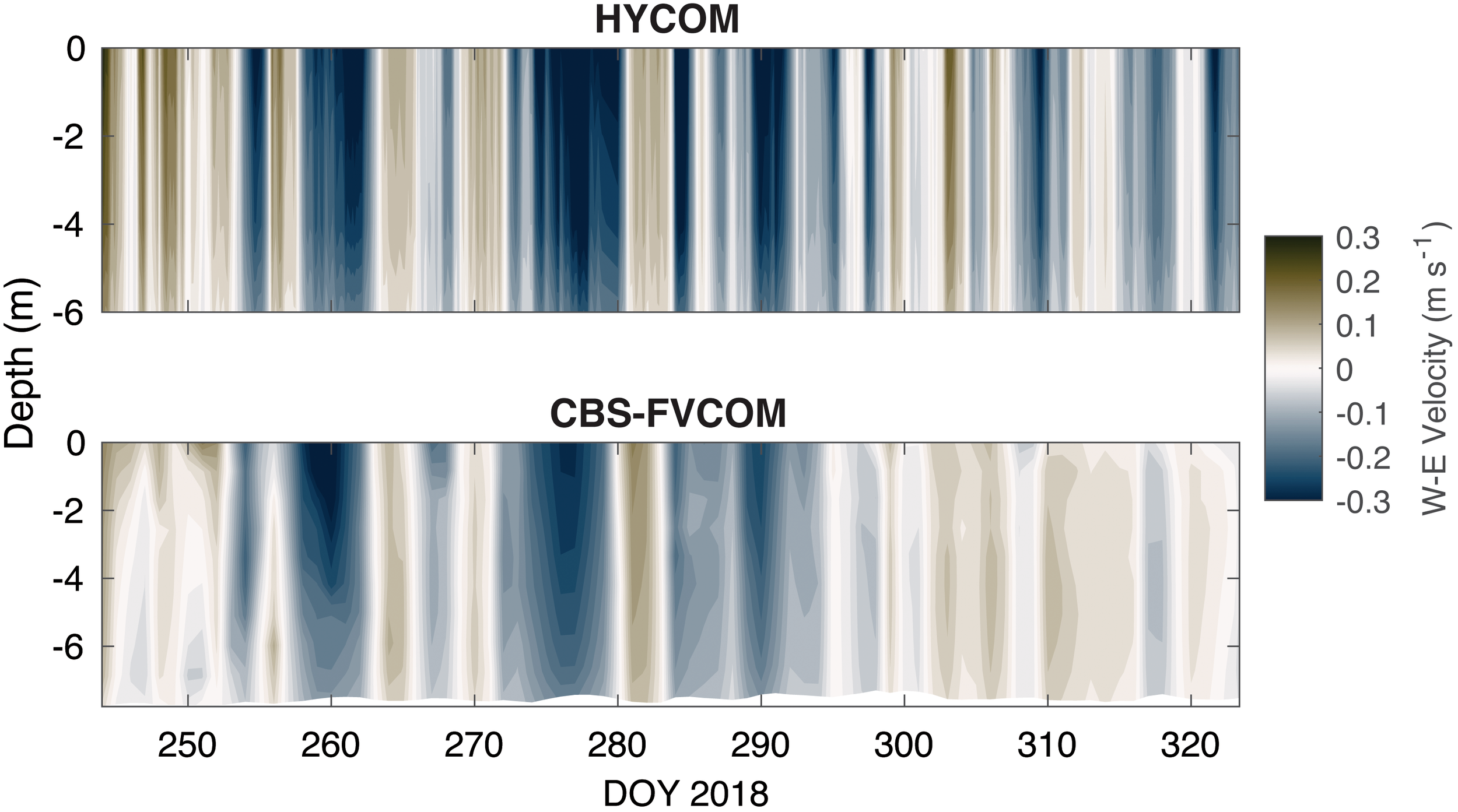
Time–depth contour plots u current velocity from CBS-FVCOM and the Navy Global HYCOM model at the closest matched grid cells for each over the fall of 2018. CBS-FVCOM, Coastal Beaufort Sea Finite Volume Community Ocean Model.
Figure 14
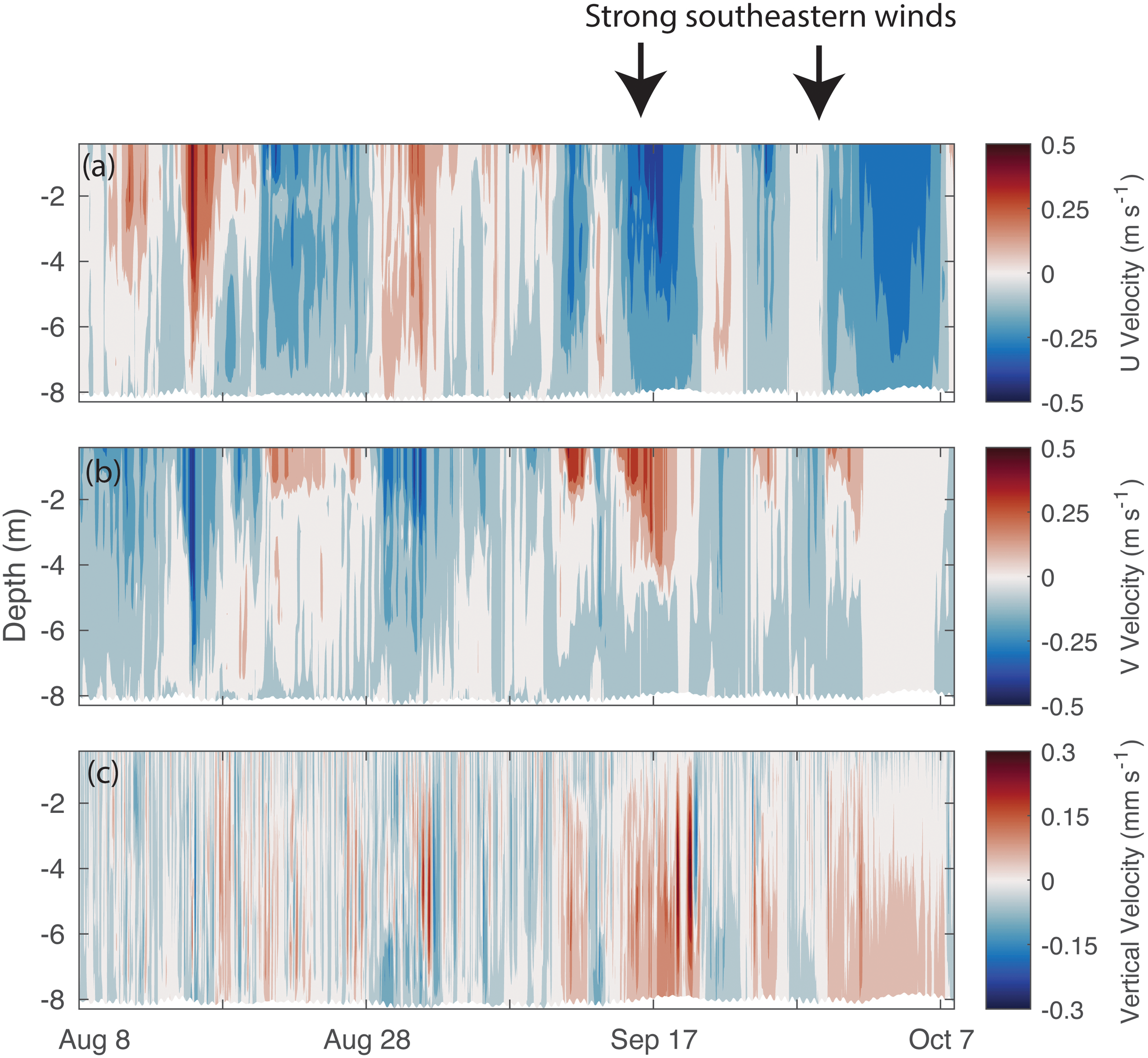
Time–depth contour plots of modeled (a)u velocity, (b)v velocity, and (c) vertical velocity at the model element center closest to the Stefansson Sound Mooring. Positive u velocity is to the east, positive v velocity is to the north (offshore), and positive vertical velocity is upward. Note that the units for vertical velocity are in mm s−1, while the others are in m s−1.
5 Model strengths, areas for improvement, and further research
5.1 Strengths
The model was adept at predicting the seasonal progression of T across years as indicated by the comparison of modeled vs. observed T in Prudhoe Bay. In addition, SSH was extremely well represented at Prudhoe Bay, and tidal and sub-tidal variability was recreated across stations where measurements were available. Limited observations of the vertical distribution of S collected during cruises in 2021 and 2022 also showed that the model captured first-order changes in S stratification in nearshore environments, although the concurrent measurements of T were not as well recreated (Figure 5). There was hardly any bias in the predictions of SSH and T at Prudhoe Bay, where the longest period of observations was available for comparison, although bottom water T did not reach those measured in situ. This indicates that on a year-to-year basis, the estimates of these basic oceanographic properties within the model are very reliable and the model is suitable for studies using the hydrodynamic solution for interannual analysis and subsequent coupling to biogeochemical simulations.
Another strength of the holistic observational-modeling system is the availability of sustained observations, providing the ability for future model enhancements and evaluation. At the time of model construction, only 1-year moored observations from the BLE-LTER were available for model comparison. Since then, 5 years of CTD data from Jago and Kaktovik lagoons and 2 years (2022–2023) from Stefansson Sound have been made public. This allows for the planned extension of the model in time and the potential to support future field missions as forcing data are made available and will be included in future publications. New field programs to collect additional data (Madison Smith, personal communication) will also begin in 2025, allowing the further extension of the model in time, potentially making it suitable for operational capabilities to support regional interests related to navigation, security, and local travel over ice.
5.2 Areas for improvement
Some shorter timer variations (sub-seasonal to sub-weekly) in T and S were sometimes captured (e.g., the fall of 2018 in Jago Lagoon), but often large fluctuations in observations on short time scales were not predicted. Extreme values in daily mean SSH were also not well captured generally, with the overall model SSH being dampened relative to observations (Figure 7). This suggests an improvement in model forcing to better include storm-driven events in both wind effects and boundary currents. We tested the model by forcing with the velocity at the boundary to better improve velocity predictions within the model, but no substantial improvements were observed, and it made the model setup unnecessarily complex.
The model exhibited a clear lack of ability to capture very low wintertime T in bottom waters (Figure 6) in addition to the gradual accumulation of hypersaline water in Kaktovik and Jago lagoons (Figure 10). This is highly likely due to brine formation and ejection that occur as first-year sea ice forms in the lagoons. These complex processes are not represented in the version of CICE within our model, and the minimum model water temperature is limited by a relatively simple linear relationship between T and S of T = −0.054S. Further analysis using the gsw_SA_freezing_from_t and gsw_t_freezing from the Gibbs SeaWater Oceanographic Toolbox (McDougall and Barker, 2011) to calculate the freezing temperature of seawater and the absolute salinity (SA g kg−1) of seawater at a given temperature and pressure (decibar) indicated a decoupling in these enclosed lagoons between T and S (Supplementary Material Figure S6). This can be directly compared to Figure 10. As sea ice ejects hypersaline brine that is very dense relative to the surrounding water, it sinks to the sea floor where the sensors are mounted. Bear in mind that the depth of these sensors is only 3–4 m from the surface. This sinking and subsequent stratification could insulate the brine mix from further cooling and concentration of salinity. The freezing of seawater occurs at the bottom of the ice and is salinity dependent, and we hypothesize that the insulation of the water from further cooling and slowing the growth rate of ice limits the upper concentration of brine over the winter before spring melt. As a thought experiment, if winter continued indefinitely and the brine reached the eutectic point of a seawater mixture (T = −36.2°C), only then would it begin to freeze, and the salinity of this nominally small pool of water would be ~250 g kg−1 (Vancoppenolle et al., 2019). This would lead to a fully frozen water column with a thin layer of highly saline water at the bottom, a condition that clearly did not exist in the lagoons and was not modeled. Clearly, to represent these processes of first-year ice formation in these shallow lagoons, the CICE code within this version of the FVCOM 4.3 should be updated to the most recent. We saw a limited ability to capture observed bottom water velocity at the moorings, although there were time periods where the model better matched the observations. Li et al. (2024) provided a detailed analysis of the interaction between wind and water flow in a lagoon to the west of our domain, clearly showing the complexity of these regions that are confined, have multiple flow pathways, and are shielded from the open ocean barrier islands. One improvement to test in the future is to increase model layers (Li et al., 2024, used 40 layers relative to our 10), but that substantially increases model run time. The inability of the model to recreate this phenomenon may be due to multiple factors, such as the model parameterization of turbulent processes, numerical diffusivity, or limiting the number of vertical layers in the model to 10. Our goal was to set up a new system that can uniquely capture the interannual variability from rivers to the continental shelf, and not to specifically diagnose drivers of water current velocity at a fine scale. However, we acknowledge that water current velocity is the ultimate driver of constituent distribution, sediment erosion and deposition, and coastal erosion (Piliouras et al., 2023). A targeted study with a smaller nested model with high vertical resolution is warranted to better understand the response of water currents to varying wind regimes and storms at the lagoon sites within the model domain.
The uniform bathymetry < 1.5 m was also a limitation in this first version of the CBS-FVCOM. We have since updated the bathymetry with high-resolution bathymetric data (Zimmermann et al., 2022) that were published after the initial model setup, although preliminary results with the new bathymetry show little change in model performance with the additional bathymetric data interpolated into the model (see Supplementary Material Figure S4 for the difference in bathymetry and file stationstatistics_Run22.xls for comparison).
6 Conclusions and future work
The CBS-FVCOM system serves as the backbone for a coupled hydrodynamic–ecosystem model that is currently being tested and run to simulate nutrients, carbon, phytoplankton, multiple classes of organic and inorganic sediment, and inherent optical properties. Linking a high-resolution coastal ocean model to regional and global models could offer a better methodology for understanding how regional coastal processes affect basin scale dynamics. This modeling system allows a direct link, without coarse parameterization, to include nearshore processes. This has implications for erosion, navigation, security, infrastructure stability, directly understanding how rivers, both large and small, mix in the ocean, and numerous other processes that a model that is regional or global parameterizes at best or ignores entirely.
Additionally, the future potential to link with a land surface model of the region (e.g., Rawlins, 2021) would allow for a fully coupled land–river–ocean modeling system to simulate water fluxes and carbon processes from the rivers and along the shore. The addition of erosional mechanics and coastal permafrost dynamics (e.g., Repasch et al., 2024; Undzis et al., 2024) would be necessary to complete the coastal ecosystem model to simulate nearly all processes relevant from applications such as navigation and infrastructure security to long-term climate change impacts to the coastal Arctic. The ability to simulate year-round physical processes at such high spatial resolution and to resolve delta channels and shallow lagoon systems allows for a deep exploration of the changing physical–biogeochemical processes in this region of the coastal Arctic. The coastal Beaufort Sea is a region with substantial economic and cultural importance and is already seeing the potential impacts of a warming climate on phytoplankton communities (Anderson et al., 2022) in addition to the ongoing threat of erosion (Jones et al., 2009). CBS-FVCOM is poised to answer many questions moving forward, and this publication is the first step in describing the model setup.
While changes to the physical dynamics and setup within the model and expansion into past and more contemporary years are ongoing, field data and especially current velocity measurements are needed to better understand the coastal dynamics. The flow of water ultimately determines the fate of riverine-derived materials in the ocean, including how long a given parcel of water remains intact with the surface and thus able to grow phytoplankton, exchange CO2, and transport sediment. Substantial and continued investment in observation networks, from basic physics (currents, CTD, and waves) to more complex properties, is absolutely critical to have a robust and scientifically rigorous modeling system. This is a matter not just of long-term potential carbon-climate feedbacks but also of national security, food security, and cultural identity of the region. The CBS-FVCOM (version 1.0 presented here) currently provides a platform to simulate these processes in the region; we look forward to a more detailed analysis of ice formation and melting, landfast ice dynamics, biogeochemical processes, and carbon cycling in the future.
Statements
Data availability statement
The datasets presented in this study can be found in online repositories. The names of the repository/repositories and accession number(s) can be found below: https://github.com/bclark805/CBS-FVCOM/releases/tag/v1.0.0.
Author contributions
JC: Conceptualization, Data curation, Formal Analysis, Funding acquisition, Investigation, Methodology, Project administration, Resources, Software, Supervision, Validation, Visualization, Writing – original draft, Writing – review & editing. WM: Data curation, Funding acquisition, Project administration, Resources, Supervision, Writing – review & editing. AE-H: Investigation, Resources, Writing – review & editing, Methodology, Data curation. MT: Methodology, Supervision, Resources, Investigation, Writing – review & editing, Funding acquisition. KT: Data curation, Methodology, Validation, Investigation, Resources, Writing – review & editing. HW: Resources, Investigation, Data curation, Writing – review & editing. SA: Writing – review & editing, Data curation, Methodology, Funding acquisition, Writing – original draft, Resources. JS: Investigation, Writing – review & editing, Methodology, Resources.
Funding
The author(s) declare that financial support was received for the research and/or publication of this article. This research was supported by the National Aeronautics and Space Administration Ocean Biology and Biogeochemistry program #NNH20ZDA001N-OBB. A portion of J. Shermans’ work was performed and funded under ST13301CQ0050/1332KP22FNEED0042.
Acknowledgments
We would first like to acknowledge the Iñupiat people whose lands and waters this study has taken place. We also acknowledge the BLE-LTER group, especially Jim McClelland and Andy Mahoney, for help interpreting some of the data collected under the BLE-LTER program, and the National Science Foundation and LTER program for providing the data freely and in open source. We also acknowledge Dr. Antonio Mannino for providing helpful feedback throughout the study and the material support to J.B. Clark in performing the manuscript preparation and data analysis. Thank you to Captain Mike of the R/V Ukpik for the use of the vessel for data collection in 2021 and 2022. We also acknowledge three reviewers for helpful feedback in shaping this manuscript. This work would not be possible without the great staff of the NASA Goddard Space Flight Center Discover supercomputer and the High-End Computing program.
Conflict of interest
Author JS was employed by the company Global Science & Technology, Inc.
The remaining authors declare that the research was conducted in the absence of any commercial or financial relationships that could be construed as a potential conflict of interest.
Generative AI statement
The author(s) declare that no Generative AI was used in the creation of this manuscript.
Publisher’s note
All claims expressed in this article are solely those of the authors and do not necessarily represent those of their affiliated organizations, or those of the publisher, the editors and the reviewers. Any product that may be evaluated in this article, or claim that may be made by its manufacturer, is not guaranteed or endorsed by the publisher.
Supplementary material
The Supplementary Material for this article can be found online at: https://www.frontiersin.org/articles/10.3389/fmars.2025.1580690/full#supplementary-material
References
1
Ahmed R. Prowse T. Dibike Y. Bonsal B. O’Neil H. (2020). Recent trends in freshwater influx to the arctic ocean from four major arctic-draining rivers. WATER12, 1189. doi: 10.3390/w12041189
2
Anderson D. Institution W. H. O. Fachon E. Hubbard K. Lefebvre K. Lin P. et al . (2022). Harmful algal blooms in the Alaskan Arctic: An emerging threat as the ocean warms. Oceanography. 35 (3/4), 130–139. doi: 10.5670/oceanog.2022.121
3
Chassignet E. Hurlburt H. Metzger E. J. Smedstad O. Cummings J. Halliwell G. et al . (2009). US GODAE: Global ocean prediction with the HYbrid coordinate ocean model (HYCOM). Oceanography22, 64–75. doi: 10.5670/oceanog.2009.39
4
Chen C. Gao G. Qi J. Proshutinsky A. Beardsley R. C. Kowalik Z. et al . (2009). A new high-resolution unstructured grid finite volume Arctic Ocean model (AO-FVCOM): An application for tidal studies. J. Geophys. Res., C: Oceans 114 (C8). Available online at: https://onlinelibrary.wiley.com/doi/pdf/10.1029/2008JC004941.
5
Chen C. Gao G. Zhang Y. Beardsley R. C. Lai Z. Qi J. et al . (2016). Circulation in the Arctic Ocean: Results from a high-resolution coupled ice-sea nested Global-FVCOM and Arctic-FVCOM system. Prog. Oceanogr.141, 60–80. doi: 10.1016/j.pocean.2015.12.002
6
Chen C. Liu H. Beardsley R. C. (2003). An unstructured grid, finite-volume, three-dimensional, primitive equations ocean model: application to coastal ocean and estuaries. J. Atmospheric. Oceanic. Technol.20, 159–186. doi: 10.1175/1520-0426(2003)020<0159:AUGFVT>2.0.CO;2
7
Clark J. B. Mannino A. (2022). The impacts of freshwater input and surface wind velocity on the strength and extent of a large high latitude river plume. Front. Mar. Sci.8. doi: 10.3389/fmars.2021.793217
8
Clark J. B. Mannino A. Spencer R. G. M. Tank S. E. McClelland J. W. (2023). Quantification of discharge-specific effects on dissolved organic matter export from major Arctic rivers from 1982 through 2019. Global Biogeochem. Cycles. 37 (8), e2023GB007854. doi: 10.1029/2023gb007854
9
Clark J. B. Mannino A. Tzortziou M. Spencer R. G. M. Hernes P. (2022). The transformation and export of organic carbon across an arctic river-delta-ocean continuum. J. Geophys. Res. Biogeosci.127 (12), e2022JG007139. doi: 10.1029/2022jg007139
10
Danielson S. L. Ahkinga O. Ashjian C. Basyuk E. Cooper L. W. Eisner L. et al . (2020). Manifestation and consequences of warming and altered heat fluxes over the Bering and Chukchi Sea continental shelves. Deep-Sea. Res. Part II. Topical. Stud. Oceanogr.177, 104781. doi: 10.1016/j.dsr2.2020.104781
11
Dunton K. McClelland J. (2021). “Development of Field Research Marine Infrastructure: The Beaufort Lagoon Ecosystems Long Term Ecological Research Program.” in AGU Fall Meeting Abstracts (Vol. 2021), pp. C25B–0834.
12
Dunton K. H. Weingartner T. Carmack E. C. (2006). The nearshore western Beaufort Sea ecosystem: Circulation and importance of terrestrial carbon in arctic coastal food webs. Prog. Oceanogr.71, 362–378. doi: 10.1016/j.pocean.2006.09.011
13
Egbert G. D. Erofeeva S. Y. (2002). Efficient inverse modeling of barotropic ocean tides. J. Atmospheric. Oceanic. Technol.19, 183–204. doi: 10.1175/1520-0426(2002)019<0183:EIMOBO>2.0.CO;2
14
Fairall C. W. Bradley E. F. Hare J. E. Grachev A. A. Edson J. B. (2003). Bulk parameterization of air–sea fluxes: updates and verification for the COARE algorithm. J. Climate16, 571–591. doi: 10.1175/1520-0442(2003)016<0571:BPOASF>2.0.CO;2
15
Fang M. Li X. Chen H. W. Chen D. (2022). Arctic amplification modulated by Atlantic Multidecadal Oscillation and greenhouse forcing on multidecadal to century scales. Nat. Commun.13, 1865. doi: 10.1038/s41467-022-29523-x
16
Feng D. Gleason C. J. Lin P. Yang X. Pan M. Ishitsuka Y. (2021). Recent changes to Arctic river discharge. Nat. Commun.12, 6917. doi: 10.1038/s41467-021-27228-1
17
Gao G. Chen C. Qi J. Beardsley R. C. (2011). An unstructured-grid, finite-volume sea ice model: Development, validation, and application. J. Geophys. Res.116 (C8). doi: 10.1029/2010jc006688
18
George J. C. C. Huntington H. P. Brewster K. Eicken H. Norton D. W. Glenn R. (2004). Observations on shorefast ice dynamics in arctic alaska and the responses of the iñupiat hunting community. Arctic57, 363–374. doi: 10.14430/arctic514
19
Gibbs A. E. Richmond B. M. (2017). National assessment of shoreline change - Summary statistics for updated vector shorelines and associated shoreline change data for the north coast of Alaska, U.S.-Canadian Border to Icy Cape: U.S. Geological Survey Open-File Report 2017-1107. 21 p.
20
Grebmeier J. M. (2012). Shifting patterns of life in the Pacific Arctic and sub-Arctic seas. Annu. Rev. Mar. Sci.4, 63–78. doi: 10.1146/annurev-marine-120710-100926
21
Harris C. M. McTigue N. D. McClelland J. W. Dunton K. H. (2018). Do high Arctic coastal food webs rely on a terrestrial carbon subsidy? Food Webs.15, e00081. doi: 10.1016/j.fooweb.2018.e00081
22
Hill V. J. (2008). Impacts of chromophoric dissolved organic material on surface ocean heating in the Chukchi Sea. J. Geophys. Res.113, 1875. doi: 10.1029/2007JC004119
23
Hill V. J. Zimmerman R. C. (2016). Characteristics of colored dissolved organic material in first year landfast sea ice and the underlying water column in the Canadian Arctic in the early spring. Mar. Chem.180, 1–13. doi: 10.1016/j.marchem.2016.01.007
24
Hunke E. Allard R. Bailey A. B. Blain P. Craig A. Dupont F. et al . (2024). “Cice-consortium/cice: CICE Version 6.6.0” (Zenodo). doi: 10.5281/zenodo.14188742
25
Hunke E. C. Lipscomb W. H. (2006). CICE: The Los alamos sea ice model documentation and software user’s manual, report (Los Alamos, N. M: Los Alamos Natl. Lab.). doi: 10.1038/s41597-020-0520-9
26
Jakobsson M. Mayer L. A. Bringensparr C. Castro C. F. Mohammad R. Johnson P. et al . (2020). The international bathymetric chart of the arctic ocean version 4.0. Sci. Data7, 176. doi: 10.1038/s41597-020-0520-9
27
Jolliff J. K. Kindle J. C. Shulman I. Penta B. Friedrichs M. A. M. Helber R. et al . (2009). Summary diagrams for coupled hydrodynamic-ecosystem model skill assessment. J. Mar. Syst.76, 64–82. doi: 10.1016/j.jmarsys.2008.05.014
28
Jones B. M. Arp C. D. Jorgenson M. T. Hinkel K. M. Schmutz J. A. Flint P. L. (2009). Increase in the rate and uniformity of coastline erosion in Arctic Alaska. Geophys. Res. Lett.36 (3). doi: 10.1029/2008gl036205
29
Lantuit H. Pollard W. H. (2008). Fifty years of coastal erosion and retrogressive thaw slump activity on Herschel Island, southern Beaufort Sea, Yukon Territory, Canada. Geomorphology95, 84–102. doi: 10.1016/j.geomorph.2006.07.040
30
Lemieux J.-F. Dupont F. Blain P. Roy F. Smith G. C. Flato G. M. (2016). Improving the simulation of landfast ice by combining tensile strength and a parameterization for grounded ridges. J. Geophys. Res. C.: Oceans.121, 7354–7368. doi: 10.1002/2016JC012006
31
Lemieux J.-F. Tremblay L. B. Dupont F. Plante M. Smith G. C. Dumont D. (2015). A basal stress parameterization for modeling landfast ice. J. Geophys. Res. C.: Oceans.120, 3157–3173. doi: 10.1002/2014JC010678
32
Li C. Huang W. Chen C. Boswell K. M. Wu R. (2024). Modes of weather system-induced flows through an arctic lagoon. J. Mar. Sci. Eng.12, 767. doi: 10.3390/jmse12050767
33
Lin Y. Fujisaki-Manome A. Anderson E. J. (2022). Simulating landfast ice in lake superior. J. Mar. Sci. Eng.10, 932. doi: 10.3390/jmse10070932
34
Linke S. Lehner B. Ouellet Dallaire C. Ariwi J. Grill G. Anand M. et al . (2019). Global hydro-environmental sub-basin and river reach characteristics at high spatial resolution. Sci. Data6, 283. doi: 10.1038/s41597-019-0300-6
35
Lovvorn J. R. North C. A. Kolts J. M. Grebmeier J. M. Cooper L. W. Cui X (2016). Projecting the effects of climate-driven changes in organic matter supply on benthic food webs in the northern Bering Sea. Marine Ecology Progress Series, 548, 11–30.
36
Lovvorn J. R. Rocha A. R. Mahoney A. H. Jewett S. C. (2018). Sustaining ecological and subsistence functions in conservation areas: eider habitat and access by Native hunters along landfast ice. Environ. Conserv.45, 361–369. doi: 10.1017/S0376892918000103
37
Mahoney A. R. Eicken H. Gaylord A. G. Gens R. (2014). Landfast sea ice extent in the Chukchi and Beaufort Seas: The annual cycle and decadal variability. Cold Regions. Sci. Technol.103, 41–56. doi: 10.1016/j.coldregions.2014.03.003
38
McClelland J. W. Déry S. J. Peterson B. J. Holmes R. M. Wood E. F. (2006). A pan-arctic evaluation of changes in river discharge during the latter half of the 20th century. Geophys. Res. Lett.33 (6). doi: 10.1029/2006GL025753
39
McClelland J. W. Townsend-Small A. Holmes R. M. Pan F. Stieglitz M. Khosh M. et al . (2014). River export of nutrients and organic matter from the North Slope of Alaska to the Beaufort Sea. Water Resour. Res.50, 1823–1839. doi: 10.1002/2013WR014722
40
McDougall T. J. Barker P. M. (2011). Getting started with TEOS-10 and the Gibbs Seawater (GSW) oceanographic toolbox. Scor/iapso WG127 (532), 1–28.
41
McMahon K. W. Ambrose W. G. Reynolds M. J. Johnson B. J. Whiting A. Clough L. M. (2021). Arctic lagoon and nearshore food webs: Relative contributions of terrestrial organic matter, phytoplankton, and phytobenthos vary with consumer foraging dynamics. Estuarine. Coast. Shelf. Sci.257, 107388. doi: 10.1016/j.ecss.2021.107388
42
Mellor G. L. Yamada T. (1982). Development of a turbulence closure model for geophysical fluid problem. Rev. Geophys. Space. Phys.20, 851–875. doi: 10.1029/RG020i004p00851
43
Mesinger F. DiMego G. Kalnay E. Mitchell K. Shafran P. C. Ebisuzaki W. et al . (2006). North American regional reanalysis. Bull. Am. Meteorol. Soc.87, 343–360. doi: 10.1175/BAMS-87-3-343
44
Metzger E. J. Smedstad O. M. Thoppil P. G. Hurlburt H. E. Cummings J. A. Wallcraft A. J. et al . (2014). US navy operational global ocean and arctic ice prediction systems. Oceanography27, 32–43. doi: 10.5670/oceanog.2014.66
45
Morley S. K. Brito T. V. Welling D. T. (2018). Measures of model performance based on the log accuracy ratio. Space. Weather.16, 69–88. doi: 10.1002/2017SW001669
46
Nash J. E. Sutcliffe J. V. (1970). River flow forecasting through conceptual models part I — A discussion of principles. J. Hydrol.10, 282–290. doi: 10.1016/0022-1694(70)90255-6
47
Nielsen D. M. Pieper P. Barkhordarian A. Overduin P. Ilyina T. Brovkin V. et al . (2022). Increase in Arctic coastal erosion and its sensitivity to warming in the twenty-first century. Nat. Climate Change12, 263–270. doi: 10.1038/s41558-022-01281-0
48
Park H. Watanabe E. Kim Y. Polyakov I. Oshima K. Zhang X. et al . (2020). Increasing riverine heat influx triggers Arctic sea ice decline and oceanic and atmospheric warming. Sci. Adv.6 (45), eabc4699. doi: 10.1126/sciadv.abc4699
49
Peterson B. J. Holmes R. M. McClelland J. W. Vörösmarty C. J. Lammers R. B. Shiklomanov A. I. et al . (2002). Increasing river discharge to the Arctic Ocean. Science298, 2171–2173. doi: 10.1126/science.1077445
50
Piliouras A. Jones B. M. Clevenger T. Gibbs A. E. Rowland J. C. (2023). Variability in terrestrial characteristics and erosion rates on the Alaskan Beaufort Sea coast. Environ. Res. Lett.18, 114050. doi: 10.1088/1748-9326/ad04b8
51
Proshutinsky A. Kowalik Z. (2007). Preface to special section on Arctic Ocean Model Intercomparison Project (AOMIP) Studies and Results. J. Geophys. Res.112 (C4), C04S01. doi: 10.1029/2006jc004017
52
Proshutinsky A. Yang J. Krishfield R. Gerdes R. Karcher M. Kauker F. et al . (2005). Arctic ocean study: Synthesis of model results and observations. Eos86, 368–371. doi: 10.1029/2005EO400003
53
Qi D. Wu Y. Chen L. Cai W.-J. Yu S. Ouyang Z. et al . (2024). Rapid acidification of the arctic Chukchi Sea waters driven by anthropogenic forcing and biological carbon recycling. Geophys. Res. Lett.51 (19), e2024GL109986. doi: 10.1029/2024gl109986
54
Rantanen M. Karpechko A. Y. Lipponen A. Nordling K. Hyvärinen O. Ruosteenoja K. et al . (2022). The Arctic has warmed nearly four times faster than the globe since 1979. Commun. Earth Environ.3, 1–10. doi: 10.1038/s43247-022-00498-3
55
Rawlins M. A. (2021). Increasing freshwater and dissolved organic carbon flows to Northwest Alaska’s Elson lagoon. Environ. Res. Lett.: ERL.16, 105014. doi: 10.1088/1748-9326/ac2288
56
Repasch M. Arcuri J. Overeem I. Anderson S. P. Anderson R. S. Koch J. C. (2024). “Impacts of convective storms on runoff, erosion, and carbon export in a continuous permafrost landscape,” in Proceedings of the 12th International Conference on Permafrost. 341–348.
57
Serreze M. C. Barry R. G. (2011). Processes and impacts of Arctic amplification: A research synthesis. Global Planet. Change77, 85–96. doi: 10.1016/j.gloplacha.2011.03.004
58
Smith B. Pahlevan N. Schalles J. Ruberg S. Errera R. Ma R. et al . (2021). A chlorophyll-a algorithm for landsat-8 based on mixture density networks. Front. Remote Sens.1, 5. doi: 10.3389/frsen.2020.623678
59
Stow C. A. Jolliff J. McGillicuddy D. J. Jr Doney S. C. Allen J. I. Friedrichs M. A. M. et al . (2009). Skill assessment for coupled biological/physical models of marine systems. J. Mar. Syst.76, 4–15. doi: 10.1016/j.jmarsys.2008.03.011
60
Terhaar J. Lauerwald R. Regnier P. Gruber N. Bopp L. (2021). Around one third of current Arctic Ocean primary production sustained by rivers and coastal erosion. Nat. Commun.12, 169. doi: 10.1038/s41467-020-20470-z
61
Undzis B. Moriarty J. M. Eidam E. Overeem I. (2024). Open water Sediment Dynamics on the Alaskan Beaufort Sea Shelf: A Numerical Modeling Study. doi: 10.22541/au.172479165.55543747
62
Vancoppenolle M. Madec G. Thomas M. McDougall T. J. (2019). Thermodynamics of sea ice phase composition revisited. J. Geophys. Res.: Oceans.124, 615–634. doi: 10.1029/2018JC014611
63
Woodgate R. A. (2018). Increases in the Pacific inflow to the Arctic from 1990 to 2015, and insights into seasonal trends and driving mechanisms from year-round Bering Strait mooring data. Prog. Oceanogr.160, 124–154. doi: 10.1016/j.pocean.2017.12.007
64
Zhou W. Leung L. Lu J. (2024). Steady threefold Arctic amplification of externally forced warming masked by natural variability. Nat. Geosci. 17 (6), 508–515. doi: 10.1038/s41561-024-01441-1
65
Zimmermann M. Erikson L. H. Gibbs A. E. Prescott M. M. Escarzaga S. M. Tweedie C. E. et al . (2022). Nearshore bathymetric changes along the Alaska Beaufort Sea coast and possible physical drivers. Continental. Shelf. Res.242, 104745. doi: 10.1016/j.csr.2022.104745
Summary
Keywords
coastal processes, Arctic Ocean, river-ocean interactions, hydrodynamic modeling, polar processes
Citation
Clark JB, Moses W, El-Habashi A, Tzortziou M, Turner KJ, Waga H, Ackelson S and Sherman J (2025) A new high-resolution hydrodynamic model for the coastal Beaufort Sea in the Arctic Ocean: model construction and evaluation. Front. Mar. Sci. 12:1580690. doi: 10.3389/fmars.2025.1580690
Received
20 February 2025
Accepted
09 June 2025
Published
14 July 2025
Volume
12 - 2025
Edited by
Simone Bonamano, University of Tuscia, Italy
Reviewed by
Bo-Shian Wang, National Academy of Marine Research (NAMR), Taiwan
Daniele Piazzolla, Foundation Euro-Mediterranean Center on Climate Change (CMCC), Italy
Updates
Copyright
© 2025 Clark, Moses, El-Habashi, Tzortziou, Turner, Waga, Ackelson and Sherman.
This is an open-access article distributed under the terms of the Creative Commons Attribution License (CC BY). The use, distribution or reproduction in other forums is permitted, provided the original author(s) and the copyright owner(s) are credited and that the original publication in this journal is cited, in accordance with accepted academic practice. No use, distribution or reproduction is permitted which does not comply with these terms.
*Correspondence: J. Blake Clark, blake.clark@nasa.gov; bclark@umbc.edu
Disclaimer
All claims expressed in this article are solely those of the authors and do not necessarily represent those of their affiliated organizations, or those of the publisher, the editors and the reviewers. Any product that may be evaluated in this article or claim that may be made by its manufacturer is not guaranteed or endorsed by the publisher.