Abstract
Introduction:
High-resolution sonar systems are critical for underwater robots to obtain precise environmental perception. However, the computational demands of processing sonar imagery in real-time pose significant challenges for autonomous underwater vehicles (AUVs) operating in dynamic environments. Current segmentation methods often struggle to balance processing speed with accuracy.
Methods:
We propose a novel YOLO-based segmentation framework featuring: (1) A lightweight backbone(ghostnet) network optimized for sonar imagery processing (2) A bypass BiLSTM network for temporal feature learning across consecutive frames. The system processes non-keyframes by predicting semantic vectors through the trained BiLSTM model, selectively skipping computational layers to enhance efficiency. The model was trained and evaluated on a high-resolution sonar dataset collected using an AUV-mounted Oculus MD750d multibeam forward-looking sonar in two distinct underwater environments.
Results:
Implementation on Nvidia Jetson TX2 demonstrated significant performance improvements. (1) Processing latency reduced to 87.4 ms (keyframes) and 35.3 ms (non-keyframes)(2)Maintained competitive segmentation accuracy compared to conventional methods and achieved low latency.
Discussion:
The proposed architecture successfully addresses the speed-accuracy trade-off in sonar image segmentation through its innovative temporal feature utilization and computational skipping mechanism. The significant latency reduction enables more responsive AUV navigation without compromising perception quality. The newly introduced dataset fills an important gap in high-resolution sonar benchmarking. Future work will focus on optimizing the keyframe selection algorithm and expanding the dataset to include more complex underwater scenarios.
1 Introduction
Underwater robots have been applied in the domain of deep-sea surveys in recent years (Soreide et al., 2006; Singh et al., 2010). As some investigations are typically concentrated in areas with complex terrains, most underwater robots are equipped with forward-looking sonars for obstacle perception (Ødegård et al., 2016). It is difficult to acquire global underwater topographic data before exploration missions, thus underwater robots are often operated within unknown and dynamic environments. In these scenarios, it is essential to employ an algorithm to identify obstacles in the forward-looking sonar (Cheng et al., 2021). The sonar imaging process is complex, and artifacts generated during signal processing can degrade the image quality (Zhang et al., 2024b). Moreover, processing sonar images requires extensive computation, making it challenging to improve real-time performance (Zhang et al., 2024c). Typical sonar image segmentation methods include those based on gray-level threshold (Weng et al., 2012; Yuan et al., 2016), features of MRF (Chen et al., 2022; Luyuan and Huigang, 2020), wavelet (Tian et al., 2020) and graphical boundary (Aleksi et al., 2020) etc. These approaches depend on artificially designed feature extractors, may fail in dynamic environments with volatile features. Deep networks can learn features adaptively from data and are widely used in image segmentation (Steiniger et al., 2022; Huy et al., 2023). YOLO (Redmon et al., 2016), a prominent deep learning framework, has maintained significant popularity since its introduction. It has been continually improved and has reached the state-of-the-art in the field of image processing (Jiang et al., 2022).
Learning-based algorithms rely on dedicated datasets for training and assessment. However, due to the constraints of cost, acquisition equipment, underwater environmental conditions, and operation methods, the existing public sonar datasets are scarce. Most of the datasets are unsuitable for general application across different tasks (Irfan et al., 2021). The existing datasets mainly focus on the recognition of small objects, and such targets pose minimal risk to the safe navigation of underwater robots. In contrast, the dataset proposed in this work is specifically designed for underwater robot obstacle avoidance. These images were acquired from different underwater environments and included various obstacle samples. This dataset serves as a benchmark for addressing path planning, navigation, and mapping challenges in underwater robotics that utilize forward-looking multi-beam sonar.
However, the limited computing capacity of the embedded devices carried by underwater robots makes it challenging to process deep networks in real-time. Therefore, lightweight networks are necessary. Certain lightweight convolutional structures can achieve model compression, such as depthwise separable convolution (Howard et al., 2017), grouped convolution (Krizhevsky et al., 2012), deformable convolution (Dai et al., 2017) etc. These works simplify the computational complexity of feature extraction by modifying the fundamental structure of convolution operations, thereby achieving network lightweighting. The computational resources required by the network are reduced by modifying the network structure, making deep networks more applicable for mobile robots. We propose a deep network suitable for underwater robots that simplifies computational complexity by leveraging temporal features and modifying the convolutional structure, leading to a lightweight design. The contributions of this work are:
-
A Dataset of Forward-looking Sonar: The dataset used in this work was collected using a forwardlooking multi-beam sonar in different underwater environments, labeled with two categories: obstacle and background noise. The sonar dataset is available for public access.
-
Lightweight Backbone: A GhostNet with SE attention modules is employed to replace the Backbone of YOLOv8, enhancing network’s accuracy while reducing its computing complexity.
-
Learning-based Temporal Module: Instead of CNNs, a BiLSTM network is used to predict semantic vectors of segmentation in consecutive sonar images. This approach skips certain convolutional layers, further enhancing the network’s speed.
The rest of this study is structured as follows: Section 2 provides a brief overview of the existing sonar datasets and segmentation algorithms. Section 3 introduces the proposed sonar datasets and lightweight segmentation network. Section 4 presents the detailed experimental results and analysis. Section 5 presents a comprehensive synthesis of the entire paper.
2 Related work
2.1 Sonar datasets
There are many famous visual image datasets, such as ImageNet (Deng et al., 2009), COCO (Lin et al., 2014), etc. However, due to the fact that sonar images often face problems such as scarcity of target samples and difficulty in acquisition, there are fewer public sonar datasets available. Most of the current public sonar datasets have certain specificities to be adapted to different tasks. For the classification task of sonar data with long-tailed distribution, Jiao et al. proposed NKSID dataset (Jiao et al., 2024) for small target detection tasks. NKSID employs a remotely operated vehicle to collect sonar data, including targets such as propellers, iron pipes, tires, and other small-scale artificial structural targets. Notably, the dataset does not include natural terrains like rocks or slopes. SCTD (Zhang et al., 2022b) and UATD (Xie et al., 2022) are both datasets that are widely applied and contain sonar images of various underwater targets. However, these two datasets mainly consist of small targets too, and do not include pixel-level segmentation labels. In the task of sonar image segmentation, the dataset (Singh and Valdenegro-Toro, 2021) encompasses various small targets such as underwater debris. This dataset comprises a substantial collection of sonar images of marine debris, meticulously annotated at the pixel level. Nonetheless, the sonar images in this dataset were captured within a tank environment, which struggles to replicate the intricate actual underwater conditions. In summary, the existing sonar datasets primarily focus on small targets, and there are fewer sonar datasets for segmentation of large topographical obstacles which affect the navigation safety of the underwater robots.
2.2 YOLO based networks
YOLO network has undergone multiple versions, achieving a significant performance in both speed and accuracy. Many researchers have focused on lightweighting the YOLO network. Zheng et al. introduced adaptive anchor boxes to incorporate prior information into the YOLO network, achieving satisfactory accuracy. However, their method primarily focuses on algorithmic accuracy, sacrificing processing speed, which results in slower inference when processor capability is limited (Zheng et al., 2023). Wang et al. proposed the PEP module, which reduces the parameters of the YOLO network and achieves promising results in underwater video target recognition (Wang et al., 2020). But the FPN structure in its network transmits semantic but not localization information, limiting its multi-scale target fusion capability. Similarly, Zhang et al. reduced the latency of the YOLOv5 model by 9 ms by pre-clustering annotation information from sonar images (Zhang et al., 2022a). But due to the background speckle noise in the underwater environment, some false alarms affect the accuracy of the algorithm. Xu et al. employed an adaptive attention module to capture inter-channel features and utilized depthwise separable convolutions for network lightweighting, but neglected the multi-scale features (Xu et al., 2024). For image segmentation tasks, YOLACT (Bolya et al., 2019), a segmentation network based on the YOLO architecture, employed multiple predict heads to decouple the task into classification, bounding box regression and mask prediction, achieved faster speed than Mask-RCNN (He et al., 2017) in image segmentation tasks. This network architecture has exhibited remarkable performance in the domain of visual image segmentation. Based on YOLACT, Liu et al. leveraged temporal redundancy information in continuous videos, performing feature transformation using an optical flow network. Their method achieved a 3–5x speedup compared to existing approaches on edge devices (Liu et al., 2021).
YOLOv8 (Jocher et al., 2023), proposed in 2023, integrates multiple tasks such as classification, detection, segmentation, and tracking into one project, demonstrates excellent performance on numerous public datasets. The YOLOv8 network consists of three components: Backbone, Neck and Predict head. The Backbone is used for extracting shallow spatial features. The Neck, which is composed of FPN and PAN (Liu et al., 2018), is used for fusing features of different scales. PAN adds a bottom-up fusion path, enhancing target localization and improving multi-scale fusion accuracy. The Predict head module of YOLOv8 has a similar structure to (Bolya et al., 2019; He et al., 2017) in the task of image segmentation. Figure 1 illustrates the process of image segmentation using YOLOv8. The network achieves effective image segmentation by decomposing it into two parallel tasks: prediction of prototypes and semantics. The weighted sum of the mask coefficients and prototypes, along with some subsequent post-processing, ultimately produces the network’s output.
Figure 1
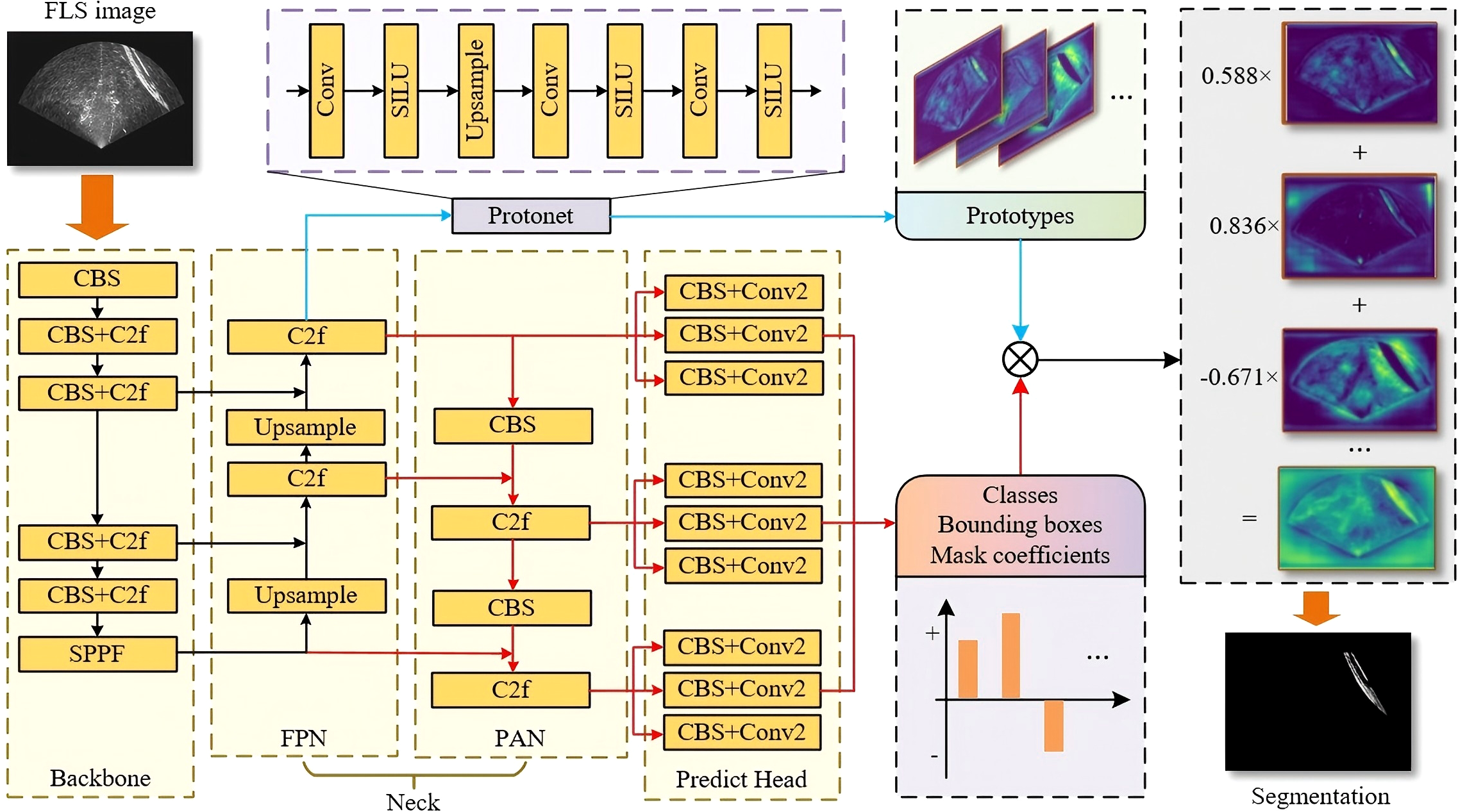
YOLOv8 segmentation network. The red arrows denote the prediction of semantics, while the blue ones denote those of prototypes.
Even the smallest version of YOLOv8 network still contains a large number of parameters. Besides, taking the YOLOv8n network (the smallest variant) as an illustration, the PAN module contains a considerable proportion of parameters (24.55%), as well as the Predict head (27.94%). These components contain a large number of parameters but produce only low-dimensional and abstract semantic information for segmentation, such as classes, bounding boxes, and mask coefficients, which affect the network’s speed. This study adopts YOLOv8n as the baseline model due to its highly lightweight architecture.
2.3 Temporal sequence prediction
There are two types of temporal sequence prediction methods in general: statistical-based and learning based. The statistical-based model have poor adaptability to non-stationary data such as the ARIMA model. BiLSTM network is a learning-based temporal prediction method that can learn bidirectional temporal features of the data (Siami-Namini et al., 2019). It achieves higher detection accuracy and adapts well to dynamic temporal features but requires more batch data for training. The BiLSTM network has extensive applications in the feature extraction of consecutive images. In the framework of (Bin et al., 2019), the BiLSTM network is used to extract temporal features from continuous images, allowing the model to make full use of the contextual semantic information over a longer period. The method demonstrates that BiLSTM possesses a robust capability for extracting continuous temporal features, although it has not been tested on sequences with unstable temporal feature variations. In (Madake et al., 2022), the BiLSTM network is effectively used as an encoder to utilize the preceding and following information of consecutive images to generate subtitles.
3 Dataset and network
3.1 High resolution sonar dataset
We propose a dedicated forward-looking sonar dataset for underwater robot obstacle segmentation and recognition. This dataset contains sonar images collected from different marine environments and conditions, with detailed annotation information for each image, including the location, category and mask of the target, making it suitable for supervised learning and evaluating for the performance of networks.
In primary work (Xu et al., 2023; Yang et al., 2023), we built an AUV that can be used for underwater archaeological surveys. As shown in Figure 2, an Oculus MD750d forward-looking sonar is integrated for data collection. This sonar has two operating frequency bands. The high-frequency mode offers higher data resolution but a shorter range, whereas the low-frequency mode is the contrary. The AUV cruised at a speed of 0.5m/s and maintained a fixed depth to acquire stable sonar images. During data acquisition, the pitch and roll angles of the AUV are both less than ±3°. In contrast to the clarity of images, the obstacle detection task pays more attention to the spatial scope of the image, therefore, we use the frequency of 750kHz to achieve a larger detection range. The sonar range was set to 100 meters.
Figure 2
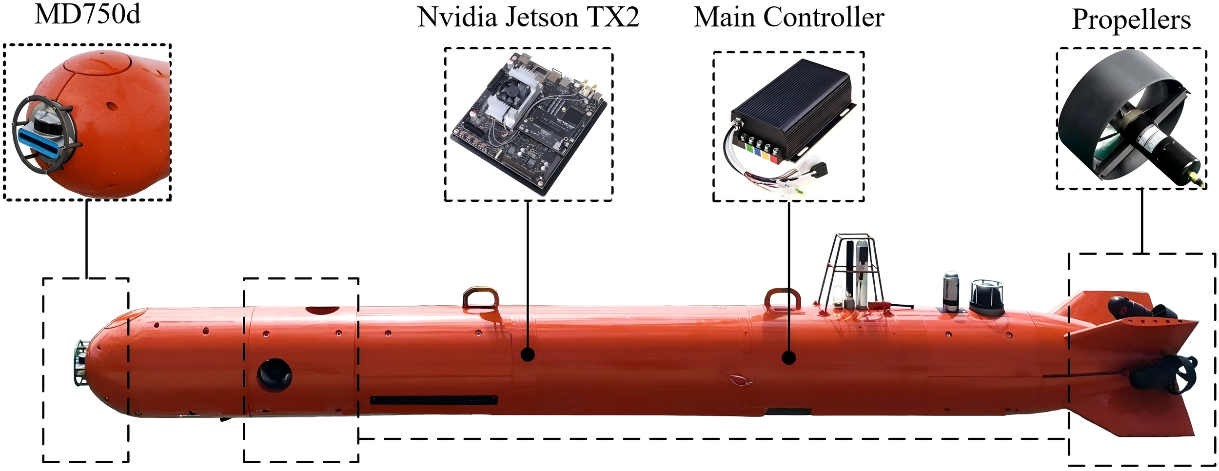
The AUV for data collection.
We collected more than 5000 forward-looking sonar images from two distinct locations in China: Qiandao Lake in Zhejiang Province and Nanshan Harbor in Hainan Province. These locations were carefully selected to ensure diversity in the dataset, representing both structured and unstructured underwater environments. As shown in Figure 3, the sonar images collected in Qiandao Lake contain rocks and slopes, while the images obtained in Nanshan Harbor include piers and vessels. By incorporating these varied environments, the dataset encompasses a broad spectrum of obstacle types, enhancing its applicability to real-world underwater navigation scenarios. Structured obstacles, such as piers and vessels, have defined geometric shapes and predictable sonar reflections, whereas unstructured obstacles, like rocks and sloped surfaces, exhibit irregular contours and varying sonar signatures. The combination of these elements contributes to a more comprehensive dataset, enabling underwater robots to handle diverse navigational challenges effectively.
Figure 3
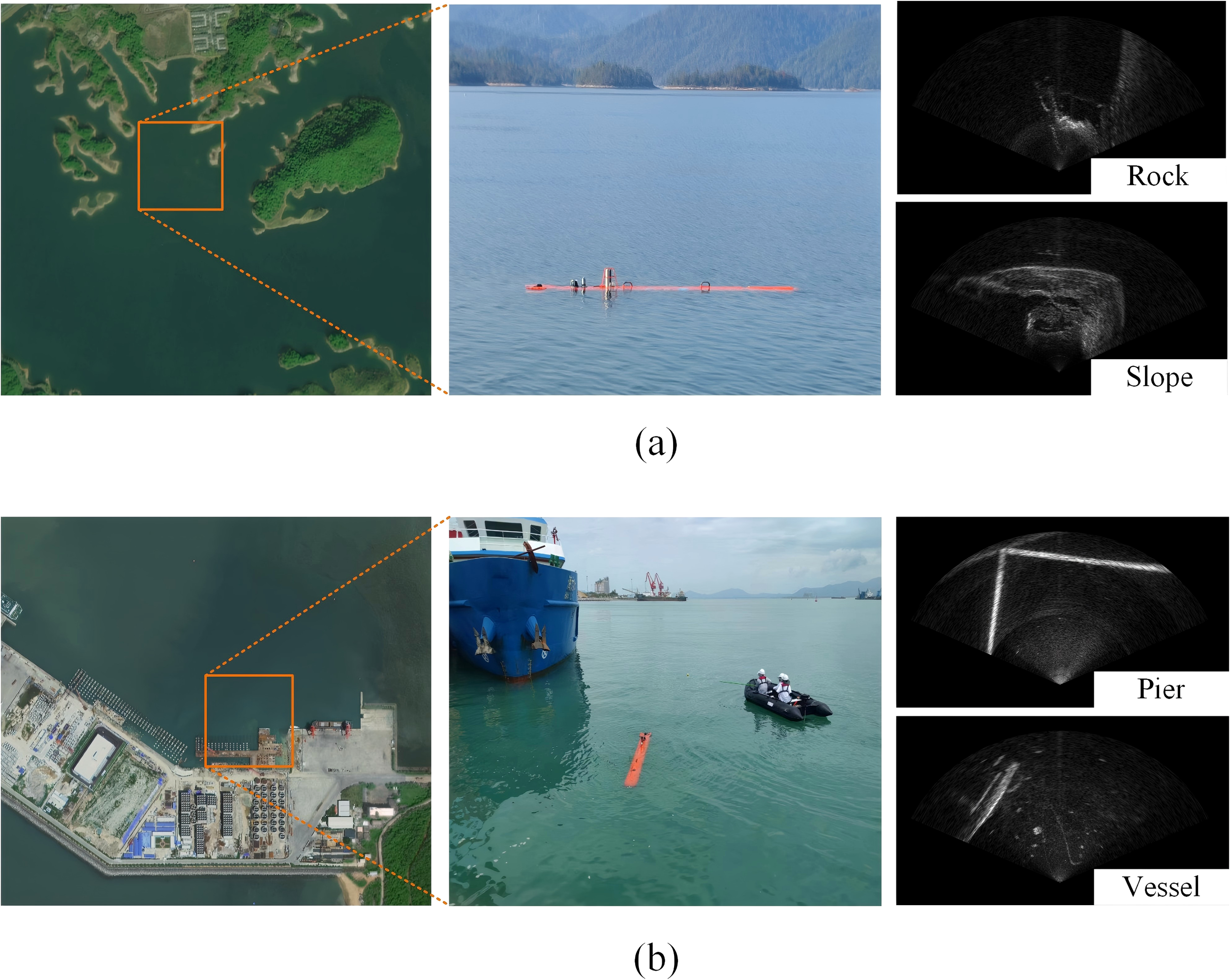
Data set and its acquisition area. (a) Qiandao Lake. (b) Nanshan Harbor.
We selected 381 sonar images containing various types of obstacles for annotation. Each image is manually labeled with instance-level class labels, corresponding bounding boxes, and segmentation masks. The sonar images are randomly split into 342 training images and 39 testing images. The class distribution across the entire dataset is relatively balanced, though minor natural imbalances exist due to variations in scene content across the two locations.
The size of each sonar image is 800 pixels×1300 pixels. Due to the acoustic reflections from the bottom, there are a lot of background noises in forward-looking sonar images. These areas are also the brighter regions in the sonar image, leading to false alarms in obstacle avoidance tasks. We labeled two classes of samples in the dataset, one is obstacle, and the other is background noise, as shown in Figure 4. The annotations are in json and txt formats. There is a yaml file located in the root directory of the dataset, which defines the root path of the dataset as well as the location of the validation subset and the training subset. The file name of the sample is the 13-bit timestamp representing the acquisition time. The distribution of the experimental dataset is shown in Figure 5. The dataset is publicly available at https://www.kaggle.com/datasets/gaoxiansen93/high-resolution-sonar-dataset.
Figure 4
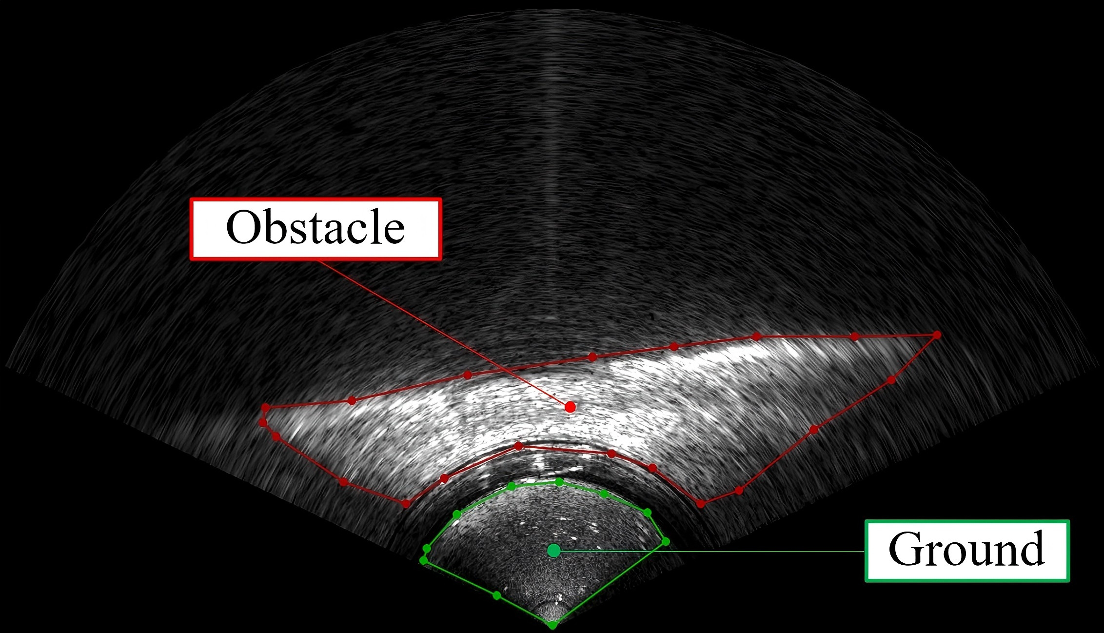
Samples labeled in dataset.
Figure 5
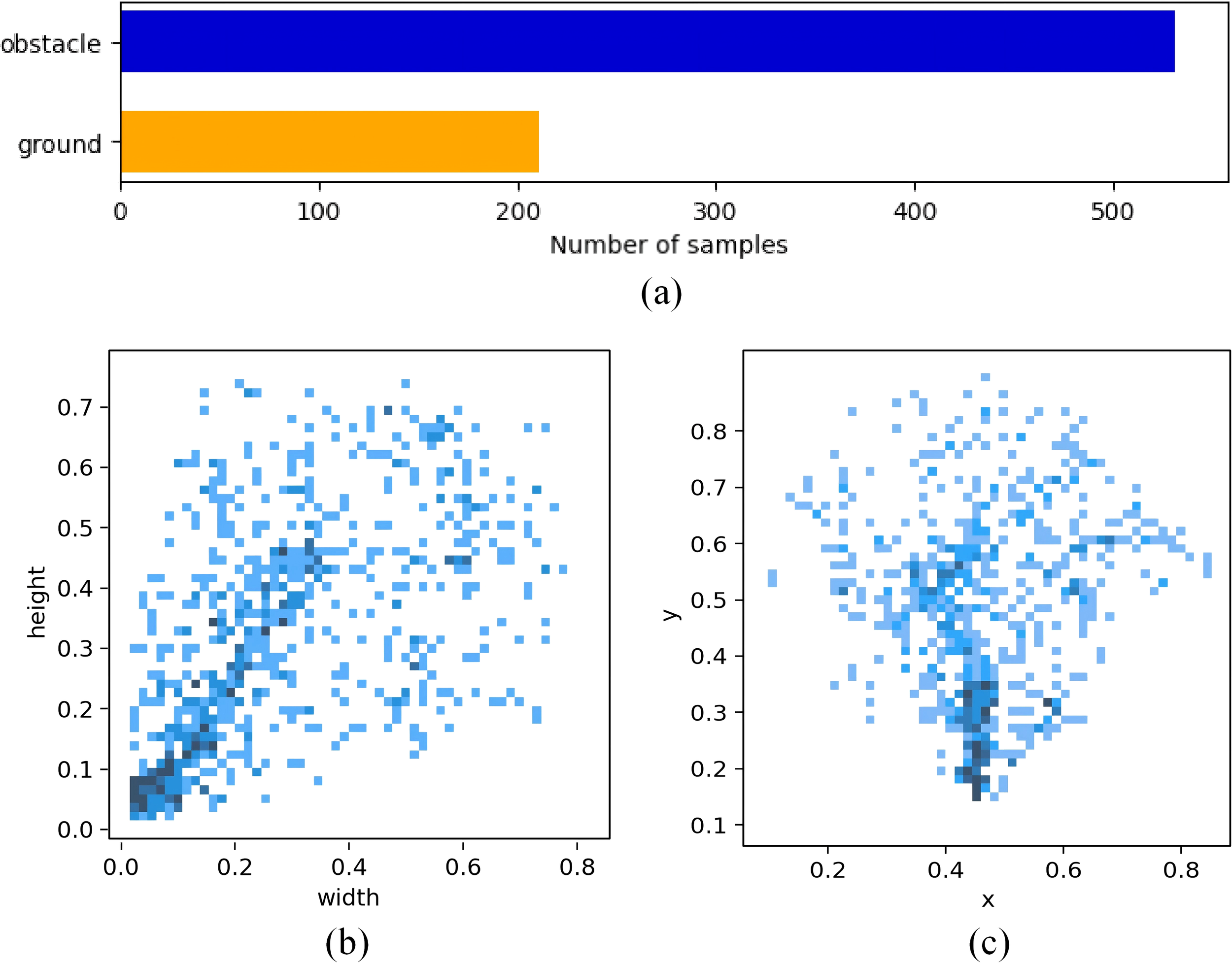
Sample distribution of the dataset. (a) Quantity of samples. (b) Size of samples. (c) Position of samples.
Structured obstacles, such as piers and vessels, typically exhibit clear geometric edges and predictable sonar reflections, while unstructured obstacles, like rocks and sloped terrain, show irregular contours and diffuse echo patterns. Furthermore, the underwater environments in these locations introduce additional complexity by including various biological entities, such as schools of fish. While these organisms do not pose a direct physical threat to the navigation of underwater robots, they can generate misleading sonar echoes, potentially triggering false alarms in obstacle detection systems. As a result, the dataset also serves as a valuable resource for developing and refining filtering techniques that can distinguish between genuine obstacles and non-threatening marine life, thereby improving the reliability and accuracy of sonar-based navigation in complex underwater settings.
3.2 Lightweight backbone
The features in sonar images are rather sparse, therefore, the computations of shallow layers can be simplified to increase the speed of the networks. The numerous convolutional layers in the Backbone of YOLOv8, though enhancing the feature extraction capability of the network, also produce a significant amount of redundant feature maps. An efficient network, GhostNet (Han et al., 2020), with fewer parameters, is used to replace the Backbone of YOLOv8 in our work, achieving higher computational speed. The concept of GhostNet is to obtain more feature maps by cheap operations. The fundamental block in GhostNet is the Ghost bottleneck, as shown in Figure 6a, which improves upon the residual block by incorporating the Ghost module. Ghost module generates features using a small number of convolution kernels and linear transformations with lower computational costs, significantly reducing the number of parameters. As shown in Figure 6c, half of the feature maps are computed through convolution, while the other half is obtained by performing depthwise convolution on the former. Each kernel in the depthwise convolutional layer contains only one channel, improving computation speed by eliminating redundant correlations between channels. The speed-up ratio of the Ghost module is expressed as Equation 1:
Figure 6
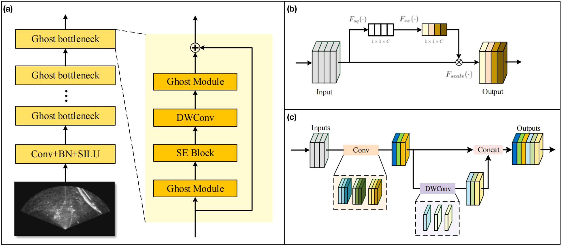
The lightweight Backbone. (a) GhostNet Backbone. (b) SE attention block. (c) Ghost Module.
where c denotes the number of channels of the input feature maps, denotes the size of output feature maps, k1, k2 denote the kernel size of intrinsic convolution and depthwise convolution, usually k1 = k2. s is the scale factor. Generally, s = 2 is chosen, which means that half of the feature maps are generated by conventional convolution, while the other half are produced using lightweight linear operations. To achieve stronger feature extraction capability, c is usually large (commonly set to 32, 64, 128, or even higher). Therefore, s ≪ c, this shows that the speed-up improvement mainly depends on s. Similarly, the compression ratio is expressed as Equation 2:
The depthwise convolutions in the Ghost module ignore the correlations among channels, leading to a decline in the network’s accuracy. The SE (Squeeze-and-Excitation) block (Hu et al., 2018) is a kind of channel-wise attention module, which extracts the correlations among channels and calibrates the feature maps. As shown in Figure 6b, the SE block consists of three processes: squeeze, excitation, and reweight.
The squeeze process compresses each feature map into 1 × 1 × C channel-wise descriptor using global average pooling. The process is expressed as Equation 3:
where uc represents a channel in the input feature maps. H × W is the size of feature maps. The excitation process associates the channel-wise descriptor zc with channel-wise weights, representing the correlations among channels. The squeeze process is expressed as Equation 4:
where and are weight matrices, is the sigmoid activation function and is the ReLU activation function, and is a hyper-parameter. Finally, The feature maps are multiplied by the channel weights, to restore its channel correlation, as Equation 5:
3.3 Semantics prediction by BiLSTM
Semantic vectors used for segmentation, such as classification scores, bounding boxes, and mask coefficients, consume a large amount of convolutional computations. We use temporal prediction to simplify the inference of semantic vectors. Inspired by (Bolya et al., 2019), we divide the forward-looking sonar data into keyframes and non-keyframes, as shown in Figure 7. For keyframes, the GhostNet-YOLOv8 model is used to segment obstacles and store the semantic vectors in data memory. For non-keyframes, the BiLSTM model predicts semantic vectors of the segmentation, allowing certain layers to be skipped. The number of parameters involved in non-keyframes is less than half of those in keyframes. In contrast to deep convolutional layers, the inference latency of the BiLSTM is negligible (less than 1 ms), thus significantly enhancing the computational efficiency of the entire network.
Figure 7
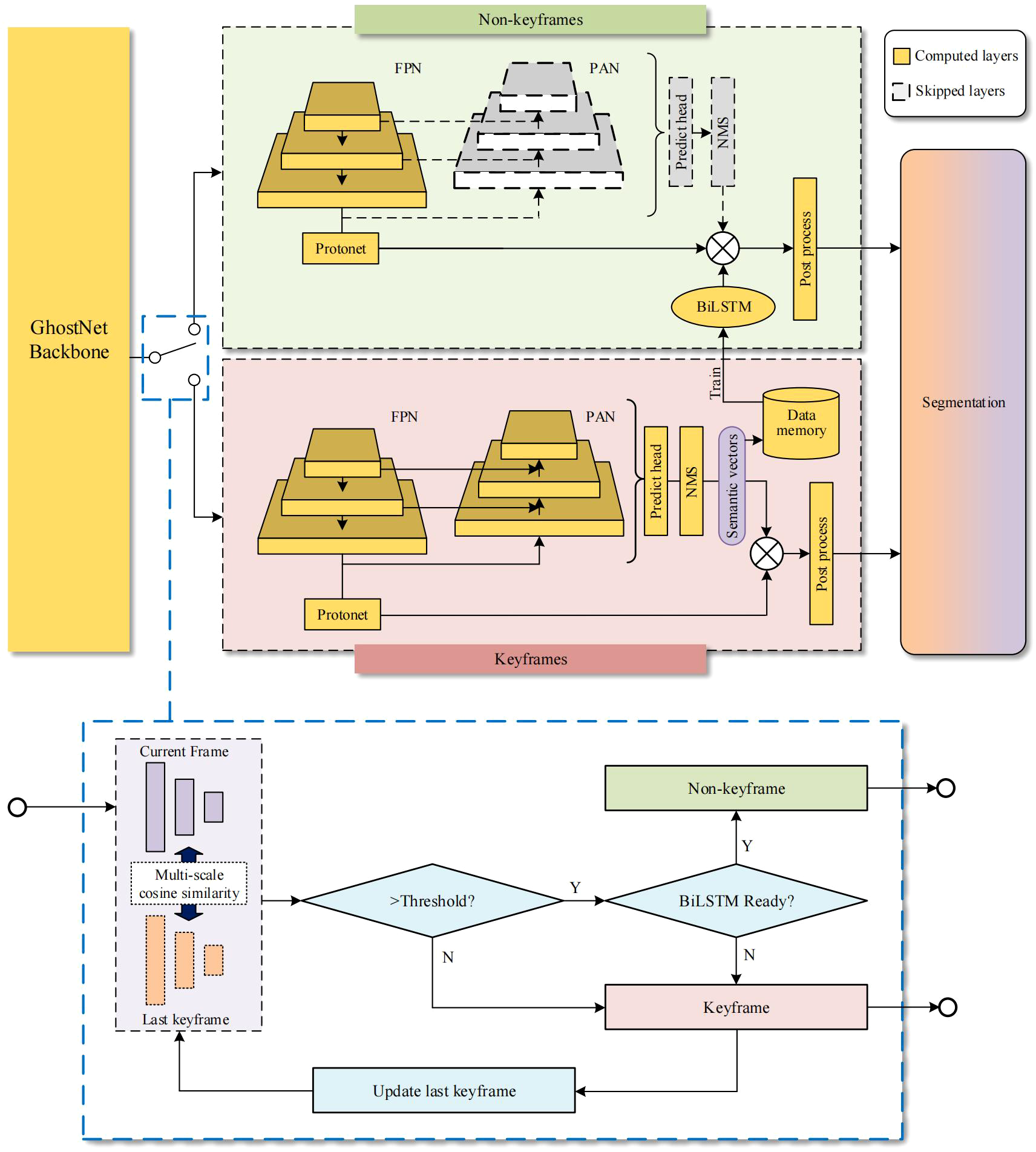
Temporal Auxiliary Network. (the yellow blocks indicate the layers that are computed, while the gray ones indicate the layers that are skipped in non-keyframes. The blue dashed box below illustrates the method of switching between keyframes and non-keyframes.).
Suppose that the sequence of input images I be divided into keyframes I(k) and non-keyframes I(n), the network is expressed as Equation 6:
where denotes the sub-network for calculating prototypes, including Backbone, FPN and Protonet. represents the sub-network for the prediction of semantic vectors, including Backbone, FPN, PAN,and Predict head. indicates the predictions of semantic vectors carried out with the BiLSTM network. The training data used for temporal feature assisted prediction has already been filtered by NMS, so no additional NMS is required during prediction.
Since underwater robots may move forward or backward, the temporal features in consecutive sonar images are bidirectional. The BiLSTM operates two LSTM networks: one in the forward direction and the other in the backward direction. The hidden states in the BiLSTM are derived from the weighted sum of the hidden states obtained from both the forward and reverse time sequences, expressed as Equation 7:
where is the semantic vectors at time , is the hidden state of the forward time sequence and is the hidden state of the backward time sequence. is the weight matrix, is the bias and is the hidden state in the BiLSTM. A fully connected layer is applied after the BiLSTM model to ensure that the output has the same dimension as semantic vectors. The Adam optimizer (Kingma and Ba, 2014) with the MSE loss function is employed to compute the gradients for updating the network parameters in BiLSTM. The Adam optimizer adjusts the learning rate through adaptive estimation of the first and second moments. By offering better stability for complex or sparse cost functions, it makes the optimization process more efficient and robust. The expression of the MSE loss function is presented as Equation 8:
Where denotes the estimation of the semantic vectors, and denotes the label of the semantic vectors.
The switching method between keyframes and non-keyframes is illustrated in the blue dashed box in Figure 7. The multi-scale cosine similarity is derived from feature maps of different sizes. It is expressed as Equation 9:
where represents the number of scales, , are the flattened feature maps of -th convolution layer in Backbone. They are respectively derived from the output feature maps of the current frame and the previous keyframe. These feature maps are reshaped into a one-dimensional format to compute their cosine similarity. When the multi-scale cosine similarity between the current image and the previous adjacent keyframe exceeds the threshold, and the BiLSTM model has been trained, the current frame is selected as a non-keyframe, and the BiLSTM is used to predict the semantic vector. Otherwise, it is treated as a new keyframe.
4 Result and discussion
4.1 Benchmarks
We utilize IoU as the metric for evaluating segmentation, it is expressed as Equation 10:
A predicted IoU greater than the threshold is regarded as a correct prediction. Otherwise, it is considered incorrect. Typically, the threshold is set to . The model’s performance is evaluated using precision and recall, as Equations 11 and 12:
where P denotes the precision, R denotes the recall, TP refers to the number of true samples correctly predicted as positive, FP refers to the number of actual positive samples incorrectly predicted as negative and FN denotes the number of true samples incorrectly predicted as negative. The mAP is a metric that combines both precision and recall, facilitating a comprehensive evaluation of the model’s performance. Its formulation is as Equation 13:
where denotes the precision of each category and indicates the recall of each category.
4.2 Experiments of lightweight backbone
We conducted an ablation experiment on the SE block with different scales of GhostNet as the Backbone. The network was deployed on the high-performance GPU, the Nvidia Jetson TX2, and the conventional CPU for a better illustration of the computational speed. The average inference latency per image was used as a metric. Besides, GFLOPs are used as a metric for quantifying the computational complexity of a model, representing the total number of floating-point operations required during inference. The results are shown in Table 1. After scaling down the parameters, the networks achieve a higher speed. However, this reduction in scale is accompanied by a corresponding decrease in mAP. While the SE block introduces additional parameters, it significantly improves the network’s performance.
Table 1
| SE block | Scale | Parameters | GFLOPs | Average latency (ms) | mAP50 | ||
|---|---|---|---|---|---|---|---|
| GPU11 | GPU22 | CPU3 | |||||
| – | ×1 | 22.2 | 9.9 | 9.4 | 103.3 | 126.7 | 0.749 |
| ✓ | ×1 | 36.0 | 10.8 | 8.9 | 105.6 | 130.0 | 0.762 |
| – | ×0.5 | 19.5 | 9.2 | 8.1 | 86.1 | 101.2 | 0.758 |
| ✓ | ×0.5 | 22.9 | 9.3 | 8.2 | 87.4 | 104.4 | 0.804 |
Ablation experiment of SE block and backbone scale.
1Nvidia GeForce RTX 3060.
2Nvidia Jetson TX2.
312th Gen Intel(R) Core(TM) i5-12490F.
Bold values indicate the best-performing methods.
A checkmark (✓) denotes the use of the SE block in the respective method, whereas a dash (–) signifies its absence.
We utilize ResNet (He et al., 2016), MobileNet (Howard et al., 2017) and EfficientVIT (Liu et al., 2023) as Backbone to conduct comparative experiments with our network. Table 2 shows mAP and latency of different computing devices. ResNet and MobileNet result in a notable enhancement in the network’s speed. However, this improvement is associated with a corresponding decline in mAP. The model utilizing GhostNet as the Backbone demonstrates superior performance in both accuracy and speed. Compared to the baseline network, the mAP50 of the model increased by 2.2%, and latency on the Nvidia Jetson TX2 was reduced by 10.6 ms.
Table 2
| Backbone | Params | GFLOPs | Average latency (ms) | mAP50 | ||
|---|---|---|---|---|---|---|
| GPU11 | GPU22 | CPU3 | ||||
| ResNet18 | 23.6 | 10.1 | 6.7 | 94.7 | 96.8 | 0.769 |
| ResNet34 | 24.3 | 10.3 | 6.9 | 97.0 | 98.3 | 0.774 |
| ResNet101 | 28.8 | 11.7 | 7.8 | 106.2 | 108.1 | 0.779 |
| MobieNet | 30.2 | 10.3 | 8.5 | 90.1 | 109.7 | 0.737 |
| EfficientVit | 28.6 | 10.2 | 19.8 | 152.3 | 121.7 | 0.775 |
| Baseline | 32.5 | 12.0 | 8.7 | 96.7 | 119.8 | 0.782 |
| Proposed | 22.9 | 9.3 | 8.2 | 87.4 | 104.4 | 0.804 |
Comparative experimental results of different backbones.
1Nvidia GeForce RTX 3060.
2Nvidia Jetson TX2.
312th Gen Intel(R) Core(TM) i5-12490F.
Bold values indicate the best-performing methods.
Figure 8a illustrates the variations in the two metrics: mAP50 and mAP50–95 of each epoch. Figure 8b shows the precision and recall at each epoch during model training. Figures 8c, d respectively illustrate the losses for the training set and validation set across each epoch. After 200 epochs, while the losses on the training set shows a slight decrease, the losses on the validation set remain stable, indicating that the model has converged.
Figure 8
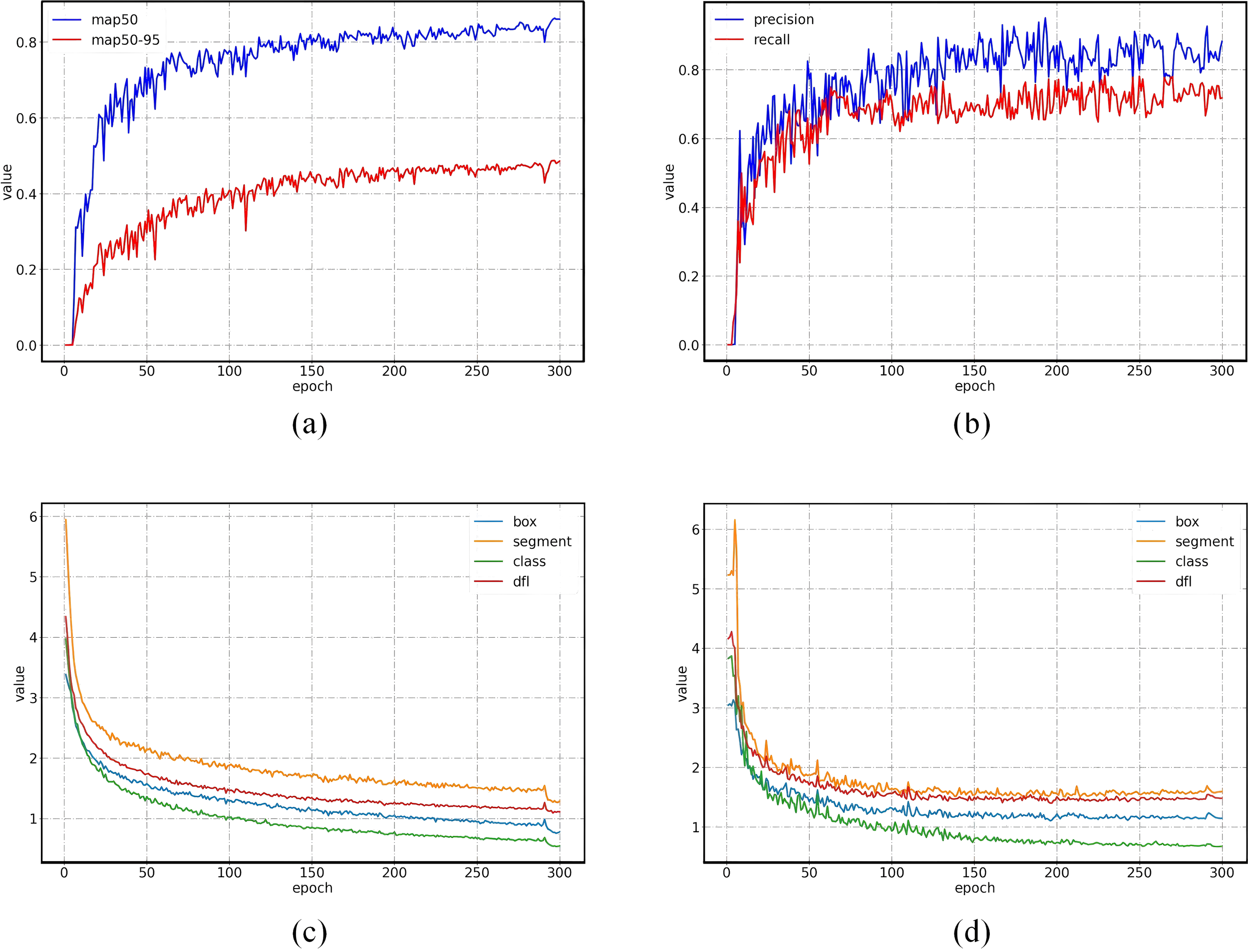
Performance and losses of each epoch. (a) mAP. (b) Precision and recall. (c) Losses on training set. (d) Losses on validation set.
Figure 9 presents the heat map generated by the Grad-CAM (Selvaraju et al., 2019) network visualization tool. In this heat map, the color gradients represent the significance or attention distribution in the original sonar image, highlighting the regions that most influence the network’s output. Warmer colors (e.g., red and yellow) correspond to areas of higher significance, while cooler colors (e.g., blue and green) indicate lower importance. When comparing the heat map from the proposed algorithm with that of the YOLOv8 network, a notable difference is observed in how the models focus on obstacle locations. The YOLOv8 network tends to exhibit a more diffuse and spread-out attention across the image, indicating that it may not always pinpoint obstacles with the same level of precision or focus. In contrast, the heat map generated by our proposed algorithm shows a more concentrated response around the positions of obstacles. This more localized focus suggests that the proposed network is better at discerning fine-grained features in sonar images and is more effective in isolating obstacles, even in complex underwater environments where the sonar reflections can be intricate and overlapping.
Figure 9
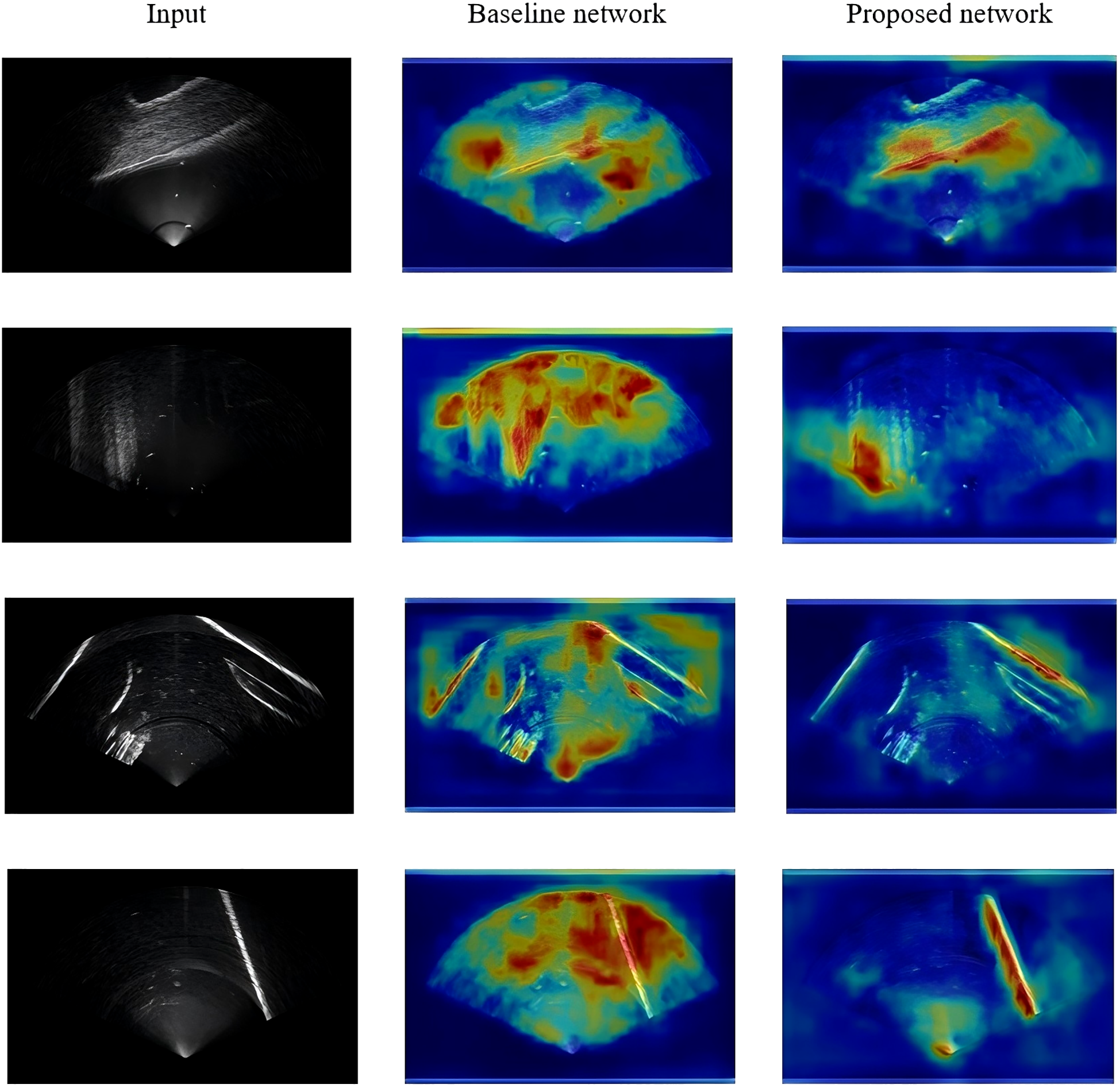
Grad-CAM Heatmaps comparison.
4.3 Semantic vector prediction
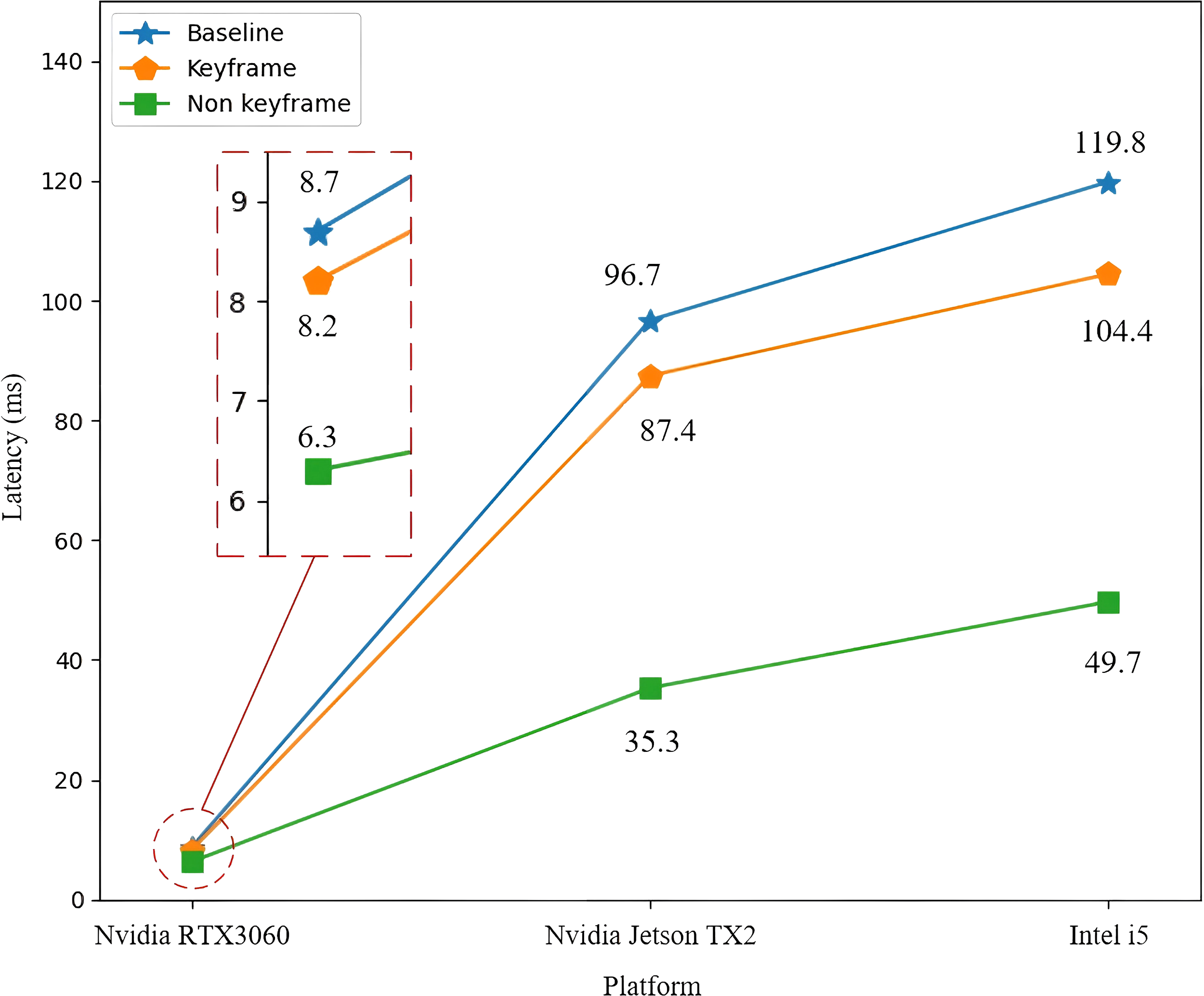
On non-keyframes, the BiLSTM model is utilized to predict semantic vectors. The loss function of the BiLSTM model for predicting semantic vectors is solved using the Adam optimizer, with the initial settings: The exponential decay rates for the first moment and the second moment are set to 0.9 and 0.999, respectively; The learning rate is set to 0.001. The network skips part of the convolutional layer, making it more lightweight. Figure 10 illustrates the comparison of computational latency among the baseline, the keyframes network, and the non-keyframes network. The improvement is more pronounced on platforms with limited computing capacity. In contrast to the keyframe network, the latency of the non-keyframe network is reduced by 61.4 ms on Nvidia Jetson TX2.
Figure 10
Latency of semantic vector prediction.
To evaluate the effectiveness of the BiLSTM model in predicting semantic vectors, we trained both LSTM and BiLSTM models using identical hyperparameters. Taking the semantic vectors predicted by the keyframe network as labels, we trained for 50 epochs on a time series dataset consisting of 200 frames. Figure 11a shows the losses of each epoch of the two models during the training process. It can be observed that, in both the training and validation sets, the loss of the BiLSTM decreases at a faster rate than that of the LSTM. We evaluated the estimation errors of LSTM and BiLSTM models on semantic vectors (including bounding box position, size, and mask coefficients) in this sequence. Errors were quantified using RMSE, and segmentation accuracy was assessed via IoU between masks predicted by keyframe models and those generated from temporal models. As shown in Figure 11b, BiLSTM provides more accurate semantic estimation, leading to lower segmentation errors than LSTM, which proves that BiLSTM has a stronger ability to extract temporal features.
Figure 11
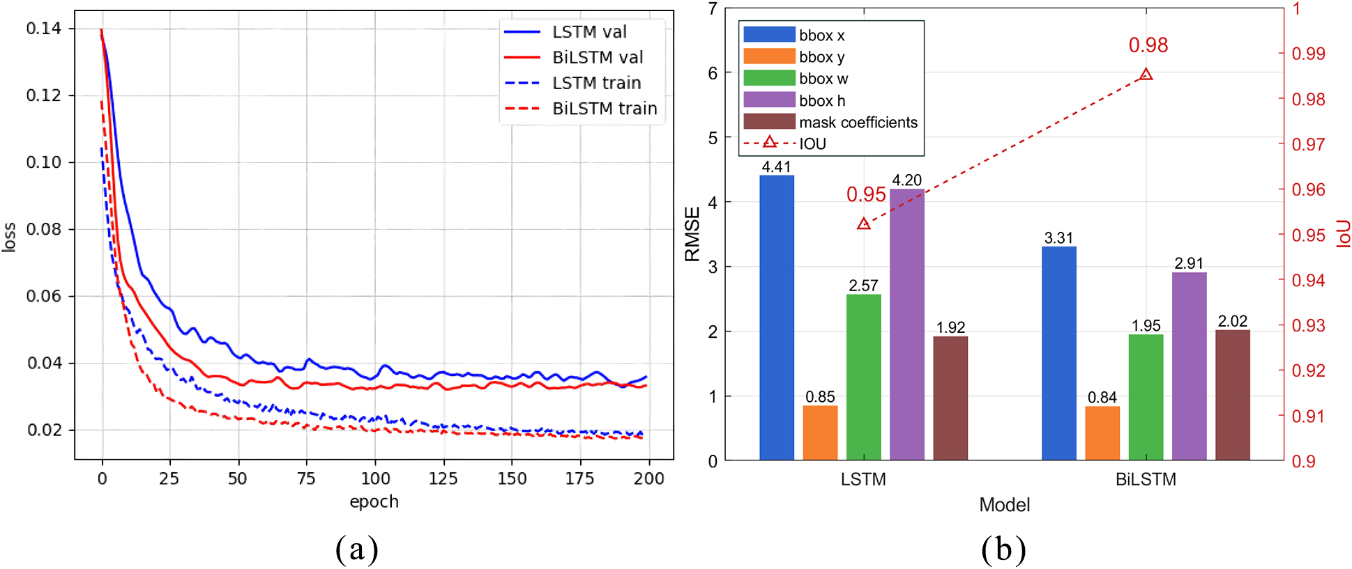
The losses and prediction errors of LSTM and BiLSTM models. (a) Losses of LSTM and BiLSTM. (b) RMSE of semantic vector prediction.
The algorithm was implemented across three sequences. As shown in Figure 12, the first row displays the original sonar image input, the second row shows the prototype generated by lightweight Backbone, and the third row shows the segmentation results obtained by predicting semantic vectors using the BiLSTM model. The fourth row illustrates the ground truth. The analysis reveals that the segmentation results from the BiLSTM model show a negligible difference compared to the ground truth. The experimental results show that BiLSTM can extract more comprehensive feature representations by combining the hidden states from both forward and backward directions, demonstrating superior capability in temporal feature extraction of mask coefficients. However, since BiLSTM requires running both forward and backward LSTM simultaneously, the model has a larger number of parameters and longer training times.
Figure 12
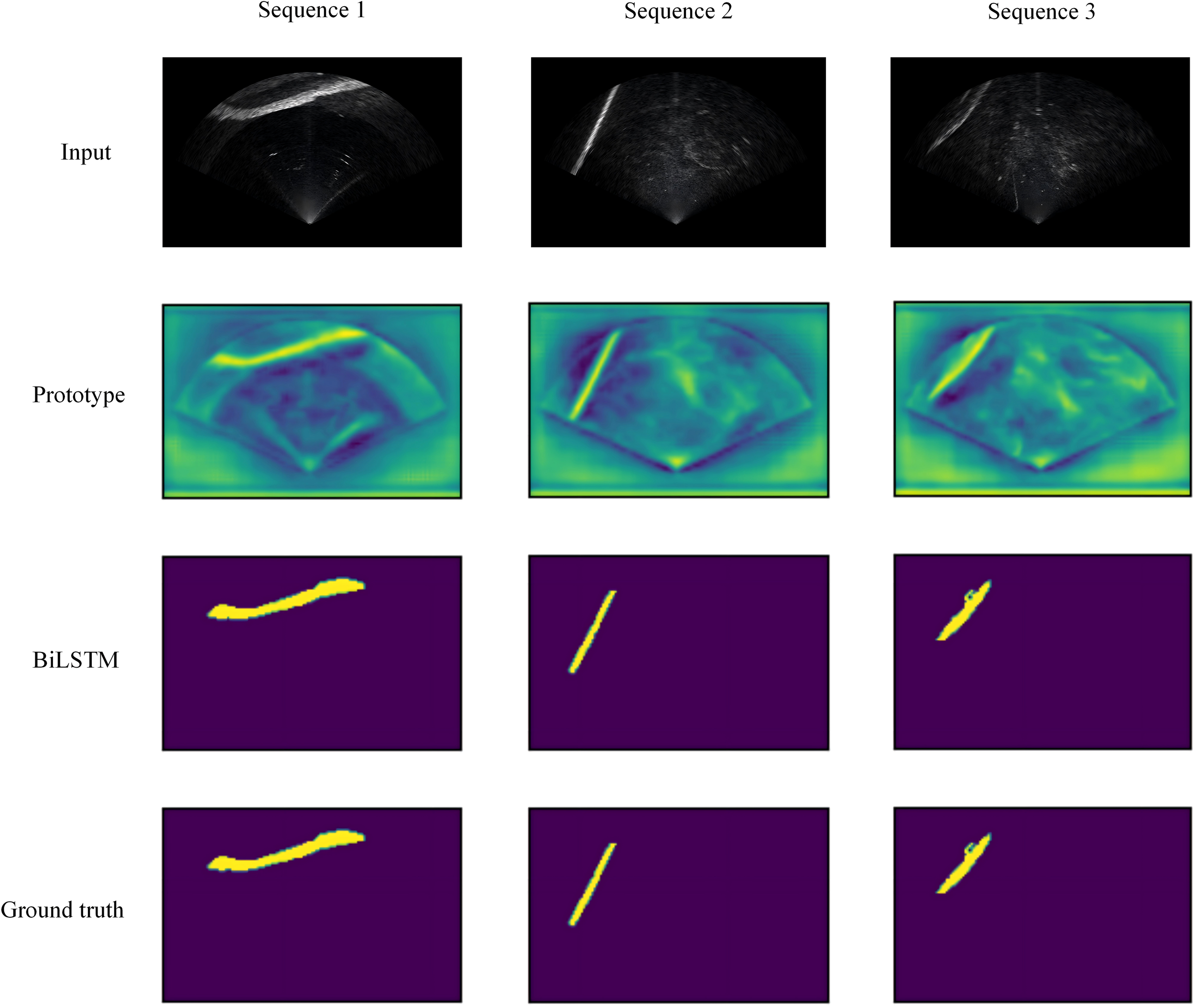
Result of segmentation in three sequences.
5 Conclusion
The forward-looking sonar dataset we propose contains a rich variety of terrain samples, making it a valuable resource for both training and evaluating sonar image processing algorithms. The dataset plays a crucial role in advancing obstacle detection and avoidance strategies for underwater robots, particularly in complex and dynamic underwater environments. By encompassing diverse obstacle types, including both structured and unstructured elements, this dataset enhances the robustness and generalization capabilities of machine learning models applied to sonar-based navigation.
Besides, we present a lightweight YOLO-based neural network tailored for deployment on embedded devices with constrained computing resources, such as those carried by underwater robots. Our approach leverages temporal features extracted from consecutive forward-looking sonar images, allowing certain convolutional layers to be skipped. This selective computation strategy significantly accelerates the network’s processing speed while maintaining a high level of precision. Furthermore, we integrate a Squeeze-and-Excitation (SE) block within the Ghost bottleneck architecture to refine feature representation. This enhancement leads to more accurate obstacle detection and segmentation, even in challenging underwater scenarios where sonar reflections may be ambiguous.
Experimental results demonstrate the effectiveness of our proposed model. Compared to the baseline network, our approach achieved a 2.2% improvement in mean Average Precision (mAP), indicating enhanced detection performance. Additionally, our model significantly reduced inference latency on the Jetson TX2 platform, achieving a speedup of 9.3 milliseconds for keyframes and 61.4 milliseconds for non-keyframes. These improvements make our method highly suitable for real-time sonar image processing on resource-limited embedded platforms.
In theory, since multibeam sonar (Ni et al., 2019), synthetic aperture sonar (Zhang et al., 2024a), and sidescan sonar (Huo et al., 2020) all contain continuous temporal information, this segmentation method is also applicable to different types of sonar images. However, due to differences in image quality and noise distribution, its accuracy may not be ideal and requires further research.
Despite these advancements, certain limitations remain. If consecutive sonar frames exhibit substantial differences due to environmental changes, sensor noise, or rapid robot movement, the performance of our model may degrade, leading to less stable detection results. Besides, in the YOLOv8 network, a semantic vector is assigned to each object, which limits the proposed method to handling a fixed number of targets.
However, in complex underwater environments, it is often difficult to determine the total number of objects in advance. In future work, we plan to incorporate a feature embedding module to align the dimensionality of semantic vectors. Additionally, achieving a balance between training efficiency and real-time inference performance remains an open research question.
Statements
Data availability statement
The datasets presented in this study can be found in online repositories. The names of the repository/repositories and accession number(s) can be found in the article/supplementary material.
Author contributions
SG: Conceptualization, Data curation, Formal analysis, Methodology, Software, Visualization, Writing – original draft, Writing – review & editing. WG: Conceptualization, Investigation, Resources, Supervision, Writing – review & editing, Writing – original draft. GX: Investigation, Project administration, Resources, Validation, Writing – original draft. BL: Formal analysis, Writing – review & editing. YS: Validation, Writing – original draft. BY: Data curation, Validation, Writing – original draft.
Funding
The author(s) declare that financial support was received for the research and/or publication of this article. This research was funded by the National Key Research and Development Program of China grant number 2023YFC2810100; The National Key Research and Development Program of China grant number 2020YFC1521704; The Youth Innovation Promotion Association of the Chinese Academy of Sciences (2023386).
Acknowledgments
This is a short text to acknowledge the contributions of specific colleagues, institutions, or agencies that aided the efforts of the authors.
Conflict of interest
The authors declare that the research was conducted in the absence of any commercial or financial relationships that could be construed as a potential conflict of interest.
Generative AI statement
The author(s) declare that no Generative AI was used in the creation of this manuscript.
Publisher’s note
All claims expressed in this article are solely those of the authors and do not necessarily represent those of their affiliated organizations, or those of the publisher, the editors and the reviewers. Any product that may be evaluated in this article, or claim that may be made by its manufacturer, is not guaranteed or endorsed by the publisher.
References
1
Aleksi I. Matić T. Lehmann B. Kraus D. (2020). Robust a*-search image segmentation algorithm for mine-like objects segmentation in sonar images. Int. J. electrical Comput. Eng. Syst.11(2), 53–66. doi: 10.32985/ijeces.11.2.1
2
Bin Y. Yang Y. Shen F. Xie N. Shen H. T. Li X. (2019). Describing video with attention-based bidirectional lstm. IEEE Trans. Cybernetics49, 2631–2641. doi: 10.1109/TCYB.6221036
3
Bolya D. Zhou C. Xiao F. Lee Y. J. (2019). Yolact: Real-time instance segmentation. In Proceedings of the IEEE/CVF international conference on computer vision. pp. 9157–9166. doi: 10.1109/ICCV43118.2019
4
Chen Z. Wang Y. Tian W. Liu J. Zhou Y. Shen J. (2022). Underwater sonar image segmentation combining pixel-level and region-level information. Comput. Electrical Eng.100, 107853. doi: 10.1016/j.compeleceng.2022.107853
5
Cheng C. Sha Q. He B. Li G. (2021). Path planning and obstacle avoidance for auv: A review. Ocean Eng.235, 109355. doi: 10.1016/j.oceaneng.2021.109355
6
Dai J. Qi H. Xiong Y. Li Y. Zhang G. Hu H. et al . (2017). Deformable convolutional networks. In Proceedings of the IEEE international conference on computer vision. pp. 764–773. doi: 10.1109/ICCV.2017.89
7
Deng J. Dong W. Socher R. Li L.-J. Li K. Fei-Fei L. (2009). “Imagenet: A large-scale hierarchical image database,” in 2009 IEEE Conference on Computer Vision and Pattern Recognition. (Miami, FL, USA: IEEE), 248–255.
8
Han K. Wang Y. Tian Q. Guo J. Xu C. Xu C. (2020). “Ghostnet: More features from cheap operations,” in 2020 IEEE/CVF conference on computer vision and pattern recognition (CVPR) (USA: IEEE), pp. 1580–1589.
9
He K. Gkioxari G. Dollar P. Girshick R. (2017). “Mask R-CNN,” in Proceedings of the IEEE International Conference on Computer Vision (ICCV).
10
He K. Zhang X. Ren S. Sun J. (2016). Deep residual learning for image recognition. In Proceedings of the IEEE conference on computer vision and pattern recognition. pp. 770–778. doi: 10.1109/CVPR.2016.90
11
Howard A. G. Zhu M. Chen B. Kalenichenko D. Wang W. Weyand T. et al . (2017). Mobilenets: Efficient convolutional neural networks for mobile vision applications. arXiv preprint arXiv:1704.04861.
12
Hu J. Shen L. Sun G. (2018). “Squeeze-and-excitation networks,” in Proceedings of the IEEE Conference on Computer Vision and Pattern Recognition (CVPR) (USA: IEEE), pp. 7132–7141.
13
Huo G. Wu Z. Li J. (2020). Underwater object classification in sidescan sonar images using deep transfer learning and semisynthetic training data. IEEE Access8, 47407–47418. doi: 10.1109/Access.6287639
14
Huy D. Q. Sadjoli N. Azam A. B. Elhadidi B. Cai Y. Seet G. (2023). Object perception in underwater environments: a survey on sensors and sensing methodologies. Ocean Eng.267, 113202. doi: 10.1016/j.oceaneng.2022.113202
15
Irfan M. Jiangbin Z. Ali S. Iqbal M. Masood Z. Hamid U. (2021). Deepship: An underwater acoustic benchmark dataset and a separable convolution based autoencoder for classification. Expert Syst. Appl.183, 115270. doi: 10.1016/j.eswa.2021.115270
16
Jiang P. Ergu D. Liu F. Cai Y. Ma B. (2022). A review of yolo algorithm developments. Proc. Comput. Sci.199, 1066–1073. The 8th International Conference on Information Technology and Quantitative Management (ITQM 2020 - 2021): Developing Global Digital Economy after COVID-19. doi: 10.1016/j.procs.2022.01.135
17
Jiao W. Zhang J. Zhang C. (2024). Open-set recognition with long-tail sonar images. Expert Syst. Appl.249, 123495. doi: 10.1016/j.eswa.2024.123495
18
Jocher G. Qiu J. Chaurasia A. (2023). Ultralytics YOLO.
19
Kingma D. P. Ba J. (2014). Adam: A method for stochastic optimization. arXiv preprint arXiv:1412.6980.
20
Krizhevsky A. Sutskever I. Hinton G. E. (2012). “Imagenet classification with deep convolutional neural networks,” in Advances in Neural Information Processing Systems, vol. 25 . Eds. PereiraF.BurgesC.BottouL.WeinbergerK. (USA: Curran Associates, Inc).
21
Lin T. Y. Maire M. Belongie S. Hays J. Zitnick C. L. (2014). “Microsoft coco: Common objects in context,” in European Conference on Computer Vision. (Zurich, Switzerland: Springer), pp. 740–755.
22
Liu H. Rivera Soto R. A. Xiao F. Jae Lee Y. (2021). “Yolactedge: Real-time instance segmentation on the edge,” in 2021 IEEE International Conference on Robotics and Automation (ICRA) (USA: IEEE). 9579–9585.
23
Liu S. Qi L. Qin H. Shi J. Jia J. (2018). “Path aggregation network for instance segmentation,” in Proceedings of the IEEE Conference on Computer Vision and Pattern Recognition (CVPR). (USA: IEEE), pp. 8759–8768.
24
Liu X. Peng H. Zheng N. Yang Y. Hu H. Yuan Y. (2023). Efficientvit: Memory efficient vision transformer with cascaded group attention. In Proceedings of the IEEE/CVF conference on computer vision and pattern recognition. pp. 14420–14430. doi: 10.1109/CVPR52729.2023.01386
25
Luyuan L. Huigang W. (2020). “Sonar image mrf segmentation algorithm based on texture feature vector,” in Global Oceans 2020: Singapore – U.S. Gulf Coast. (USA: IEEE), 1–6.
26
Madake J. Bhatlawande S. Purandare S. Shilaskar S. Nikhare Y. (2022). “Dense video captioning using BiLSTM encoder,” in 2022 3rd International Conference for Emerging Technology (INCET) (USA: IEEE), 1–6.
27
Ni H. Wang W. Ren Q. Lu L. Wu J. Ma L. (2019). “Comparison of single-beam and multibeam sonar systems for sediment characterization: results from shallow water experiment,” in OCEANS 2019 MTS/IEEE SEATTLE (IEEE). (USA: IEEE), 1–4.
28
Ødegård Ø Sørensen A. J. Hansen R. E. Ludvigsen M. (2016). A new method for underwater archaeological surveying using sensors and unmanned platforms. IFAC-PapersOnLine49, 486–493. 10th IFAC Conference on Control Applications in Marine SystemsCAMS 2016. doi: 10.1016/j.ifacol.2016.10.453
29
Redmon J. Divvala S. Girshick R. Farhadi A. (2016). “You only look once: Unified, real-time object detection,” in 2016 IEEE Conference on Computer Vision and Pattern Recognition (CVPR). (USA: IEEE), pp. 779–788.
30
Selvaraju R. R. Cogswell M. Das A. Vedantam R. Parikh D. Batra D. (2019). Grad-cam: Visual explanations from deep networks via gradient-based localization. Int. J. Comput. Vision128, 336–359. doi: 10.1007/s11263-019-01228-7
31
Siami-Namini S. Tavakoli N. Namin A. S. (2019). “The performance of lstm and bilstm in forecasting time series,” in 2019 IEEE International Conference on Big Data (Big Data). (USA: IEEE), pp. 3285–3292.
32
Singh H. Eustice R. Roman C. Pizarro O. (2010). The SeaBED AUV – a platform for high resolution imaging. Unmanned Underwater Vehicle Showcase13, 102–104.
33
Singh D. Valdenegro-Toro M. (2021). The marine debris dataset for forward-looking sonar semantic segmentation. In Proceedings of the ieee/cvf international conference on computer vision. pp. 3741–3749. doi: 10.1109/ICCVW54120.2021.00417
34
Soreide F. Jasinski M. E. Sperre T. O. (2006). Unique new technology enables archaeology in the deep sea. Sea Technol.47, 10.
35
Steiniger Y. Kraus D. Meisen T. (2022). Survey on deep learning based computer vision for sonar imagery. Eng. Appl. Artif. Intell.114, 105157. doi: 10.1016/j.engappai.2022.105157
36
Tian Y. Lan L. Guo H. (2020). A review on the wavelet methods for sonar image segmentation. Int. J. Advanced Robotic Syst.17, 172988142093609. doi: 10.1177/1729881420936091
37
Wang L. Ye X. Xing H. Wang Z. Li P. (2020). “Yolo nano underwater: A fast and compact object detector for embedded device,” in Global Oceans 2020: Singapore – U.S. Gulf Coast, 1–4. (USA: IEEE)
38
Weng L. Y. Li M. Gong Z. B. (2012). “On sonar image processing techniques for detection and localization of underwater objects,” in Advanced Technology for Manufacturing Systems and Industry, vol. 236. Applied Mechanics and Materials (Switzerland: Trans Tech Publications Ltd), 509–514.
39
Xie K. Yang J. Qiu K. (2022). A dataset with multibeam forward-looking sonar for underwater object detection. Sci. Data9, 739.
40
Xu Z. Xu D. Lin L. Song L. Song D. Sun Y. et al . (2025). Integrated object detection and communication for synthetic aperture radar images. IEEE J. Selected Topics Appl. Earth Observations Remote Sens.18, 294–307. doi: 10.1109/JSTARS.2024.3495023
41
Xu G. Zhou D. Yuan L. Guo W. Huang Z. Zhang Y. (2023). Vision-based underwater target real-time detection for autonomous underwater vehicle subsea exploration. Front. Marine Sci.10. doi: 10.3389/fmars.2023.1112310
42
Yang Y. Liang W. Zhou D. Zhang Y. Xu G. (2023). Object detection for underwater cultural artifacts based on deep aggregation network with deformation convolution. J. Marine Sci. Eng.11 (12), 2228. doi: 10.3390/jmse11122228
43
Yuan X. Martínez J.-F. Eckert M. López-Santidrián L. (2016). An improved otsu threshold segmentation method for underwater simultaneous localization and mapping-based navigation. Sensors16. doi: 10.3390/s16071148
44
Zhang P. Tang J. Zhong H. Ning M. Liu D. Wu K. (2022b). Self-trained target detection of radar and sonar images using automatic deep learning. IEEE Trans. Geosci. Remote Sens.60, 1–14.
45
Zhang H. Tian M. Shao G. Cheng J. Liu J. (2022a). Target detection of forward-looking sonar image based on improved yolov5. IEEE Access10, 18023–18034. doi: 10.1109/ACCESS.2022.3150339
46
Zhang X. Yang P. Cao D. (2024a). Synthetic aperture image enhancement with near-coinciding nonuniform sampling case. Comput. Electrical Eng.120, 109818. doi: 10.1016/j.compeleceng.2024.109818
47
Zhang X. Yang P. Wang Y. Shen W. Yang J. Wang J. et al . (2024b). A novel multireceiver SAS RD processor. IEEE Trans. Geosci. Remote Sens.62, 1–11.
48
Zhang X. Yang P. Wang Y. Shen W. Yang J. Ye K. et al . (2024c). LBF-Based CS algorithm for multireceiver SAS. IEEE Geosci. Remote Sens. Lett.21. doi: 10.1109/LGRS.2024.3379423
49
Zheng J. Zhao S. Xu Z. Zhang L. Liu J. (2023). Anchor boxes adaptive optimization algorithm for maritime object detection in video surveillance. Front. Marine Sci.10, 1290931. doi: 10.3389/fmars.2023.1290931
Summary
Keywords
lightweight network, image segmentation, autonomous underwater vehicles, forward-looking sonar, collision avoidance
Citation
Gao S, Guo W, Xu G, Liu B, Sun Y and Yuan B (2025) A lightweight YOLO network using temporal features for high-resolution sonar segmentation. Front. Mar. Sci. 12:1581794. doi: 10.3389/fmars.2025.1581794
Received
23 February 2025
Accepted
08 May 2025
Published
29 May 2025
Volume
12 - 2025
Edited by
Fausto Ferreira, University of Zagreb, Croatia
Reviewed by
Zhiping Xu, Jimei University, China
Igor Kvasić, University of Zagreb, Croatia
Updates
Copyright
© 2025 Gao, Guo, Xu, Liu, Sun and Yuan.
This is an open-access article distributed under the terms of the Creative Commons Attribution License (CC BY). The use, distribution or reproduction in other forums is permitted, provided the original author(s) and the copyright owner(s) are credited and that the original publication in this journal is cited, in accordance with accepted academic practice. No use, distribution or reproduction is permitted which does not comply with these terms.
*Correspondence: Wei Guo, guow@idsse.ac.cn
Disclaimer
All claims expressed in this article are solely those of the authors and do not necessarily represent those of their affiliated organizations, or those of the publisher, the editors and the reviewers. Any product that may be evaluated in this article or claim that may be made by its manufacturer is not guaranteed or endorsed by the publisher.