Abstract
In polar regions, the unique conditions created by sea ice coverage pose challenges for both remote sensing and in-situ observation methods. As a result, underwater acoustic detection has emerged as an effective approach for observing complex oceanic physical phenomena in these environments. Focusing on anomalies in local seawater acoustic properties caused by eddies, we propose a method for reconstructing the three-dimensional structure of eddies. An ice-edge eddy observed during the ACOBAR project serves as a case study to demonstrate the implementation of this approach. By combining an unsupervised learning strategy with B-spline surface fitting, the proposed approach reconstructs the eddy structure without relying on highly idealized axisymmetric assumptions. Using a sound speed anomaly threshold of -3 m/s to define the eddy boundaries, the reconstruction achieves an accuracy of 74%. To further assess the method’s effectiveness, the reconstructed eddy is used to simulate the eddy-induced underwater acoustic field through finite element method (FEM) modeling. The results show that this approach reduces computational time and resource consumption by more than 30%, while maintaining a mean transmission loss error of only 1.2 dB over a 20 km range. This work represents an effective integration of acoustic sensing, machine learning, and FEM simulation in oceanographic research, offering a practical and efficient solution for studying subsurface phenomena in ice-covered regions.
1 Introduction
The Fram Strait is the primary channel for water exchange between the Arctic Ocean and the Atlantic Ocean (Geyer et al., 2020; Hattermann et al., 2016; Storheim et al., 2021). It is characterized by the West Spitsbergen Current (WSC) and the East Greenland Current (EGC) (Zhao et al., 2021). The WSC transports warm, salty Atlantic Water (AW) northward along the Svalbard Islands into the Arctic Ocean, while the EGC carries cold, fresh Polar Water (PW) southward along the western side (de Steur et al., 2009). This region is influenced year-round by this distinct circulation system, which produces strong spatial gradients across the strait (Rudels et al., 1999; Schourup-Kristensen et al., 2021). These gradients contribute to the prevalence of oceanic mesoscale eddies in the region, which typically detach from the WSC and drift westward into the EGC at speeds of several kilometers per day, retaining the properties of their source water masses (Kozlov et al., 2019). Consequently, the thermohaline structure of water masses within eddies differs markedly from that outside the eddies, significantly affecting underwater acoustic propagation (Chen et al., 2022) and increasing the uncertainty of the acoustic environment in the transitional region (Timmermans and Marshall, 2020).
During the Arctic Ice Formation Period (AIFP, from September to April of the following year), uncertainty in the marine acoustic environment in the Fram Strait becomes particularly pronounced. First, eddy kinetic energy during AITP is three times greater than that during the summer period (Pnyushkov et al., 2018), and enhanced eddy activity exacerbates the unpredictability of the acoustic conditions. Moreover, extensive sea ice cover during the AIFP (Lu et al., 2023) makes mesoscale eddy detection particularly challenging. An exception is that an ice-edge eddy is detected during the AIFP of 2010 through the ACOBAR project (Geyer et al., 2023, 2022). Due to the unique Arctic environmental features, neither satellite remote sensing data nor in-situ measurements like Argo floats—commonly used to infer 0-2000m ocean properties—are available in this region. Therefore, traditional eddy detection methods such as the Contour Threshold method (Chelton et al., 2007; Nencioli et al., 2010; Xu et al., 2022), which rely on sea surface height anomalies, or composite analysis (Zhang et al., 2014, 2013) based on three-dimensional hydrographic and pressure datasets, are not applicable. This limitation hinders our understanding of polar eddies. Therefore, developing new method for eddy characterization in the Fram Strait is crucial for advancing our understanding of these phenomena.
Unlike conventional studies that focus on eddy-induced anomalies in temperature, salinity, and pressure, our research investigates the three-dimensional structure of mesoscale eddies in the Fram Strait from the perspective of their impact on underwater acoustic properties. Sound speed profiles, which are highly correlated with acoustic propagation characteristics, have been widely used to classify marine acoustic environments (Ariza et al., 2022; Jensen et al., 2012). While these studies typically divide marine environments into acoustic sub-regions, this classification approach has not yet been applied to eddy structure reconstruction.
A recent research has revealed that mesoscale eddies exhibit coherent composite patterns in terms of their sound speed anomalies (Chen et al., 2022). However, this study—like many others—relies on oversimplified assumptions, particularly the axisymmetric eddy mode (Chelton et al., 2007), which limit its applicability in realistic ocean conditions. Despite these limitations, it demonstrates the potential of acoustic data for revealing internal eddy structures. Building on this work, we propose a novel unsupervised learning strategy that classifies eddy-induced sound speed anomalies to reconstruct the three-dimensional structure of eddies in the Fram Strait during the AIFP. Compared to previous studies (Amores et al., 2017; Sandalyuk et al., 2020; Yuan et al., 2021), which primarily reconstructed eddy structures based on the assumption of axisymmetry, our method introduces two key innovations: (1) Employing the machine learning approach, which has become widely applied to oceanic eddy diffusivities prediction (Guan et al., 2022), global marine sound-scattering region classification (Ariza et al., 2022) and other oceanographic studies, eddy reconstruction is not based on the axisymmetric assumption; (2) It leverages acoustic features to reconstruct the three-dimensional boundaries of eddies using sound speed classification and B-spline surface fitting.
The proposed method is further integrated into a finite element method (FEM) modeling framework using COMSOL Multiphysics to simulate eddy-induced underwater acoustic fields. By assigning distinct density grids inside and outside the reconstructed eddy boundaries, the model achieves a significant reduction in computational time and resource usage while maintaining high simulation accuracy. This improves overall efficiency in modeling acoustic environments affected by complex eddy processes.
In this paper, we use the ice-edge eddy detected by the ACOBAR project as a case study to demonstrate the viability of identifying mesoscale eddies using sound speed anomalies and reconstructing their three-dimensional structure through our proposed methodology. The rest of paper is organized as follows: Section 2 introduces the ACOBAR project and details the detection of the ice-edge eddy, along with the data and preprocessing steps used for reconstruction. Section 3 presents the unsupervised learning framework and B-spline surface fitting approach. Section 4 analyzes the spatial distribution of physical properties inside and outside the reconstructed eddy, while Section 5 discusses the FEM-based simulation and its efficiency. Finally, Section 6 concludes the study with key findings and future outlook.
2 Data and methods
2.1 The ACOBAR project
The ACOBAR acoustic tomography experiment in central Fram Strait was carried out from September 2010 to September 2012 (Geyer et al., 2022) to develop a system for environmental monitoring of the interior of the Arctic Ocean by assimilation of data obtained with acoustic methods (https://acobar.nersc.no/). As shown in Figures 1a–c, the project detected an ice-edge eddy trapped with negative sound speed anomaly (SSA) water mass from September 5,2010 to September 15,2010 by analyzing the difference in sound speed profile (SSP).
Figure 1
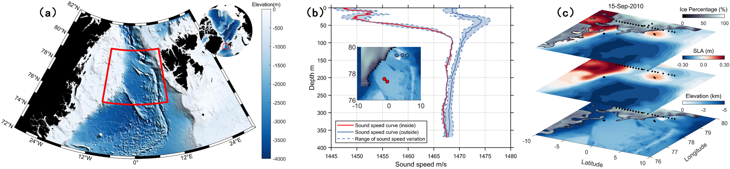
(a) The map of the Fram Strait region, the red box is the area we study. (b) The red and blue dots are five observation stations of the ACOBAR project in the ice-free region. The solid red and blue curves show the corresponding mean sound speed profiles (SSPs), while the blue dashed curves illustrate the range of sound speed variability. (c) Sea ice, sea surface level anomaly (SLA), and seafloor topography in the study area on September 15, 2010. The black dots represent all the observation stations in ACOBAR project. The top layer represents the combination of sea ice (Black-White color) and SLA (Blue-Red color); the middle layer represents the SLA, and the lower layer represents the seafloor topography (White-Blue color).
In Figure 1b, the red dots correspond to the red curve, while the blue dots correspond to the blue curve. The distribution patterns of these curves reveal an unexpected phenomenon: the measured sound speed profile (SSP) near 78°N is significantly lower than that near 80°N. Although the difference diminishes with depth, it remains noticeable within the upper 350 meters. These measurements, obtained from the ACOBAR project, challenge the widely accepted understanding that upper-ocean temperature—and, by extension, sound speed—generally decreases with increasing latitude. This anomaly suggests the possible presence of an unusually cold water mass converging near 0°E, 78°N.
2.2 The HYCOM model data
However, the limited volume of data collected by the ACOBAR project can merely help us to diagnose whether the uncommon colder water mass exists or not, it is insufficient to determine the causes of the unexpected phenomenon. Therefore, Hybrid Coordinate Ocean Model (HYCOM), which uses Navy Coupled Ocean Data Assimilation (NCODA) system (Cummings, 2005; Wang et al., 2021) for data assimilation, are selected for further analysis.
The data derived from the HYCOM (https://www.hycom.org) model include temperature, salinity, depth and SLA. The model spatial resolution is 1/12°×1/12° and the temporal resolution is 3h. Interpolation is used to determine the value between data points, contributing to continuous variations in the ocean field and the 40 layers of the vertical resolution range from 5 m at the sea surface to 5000m at the bottom. Table 1 displays the details of the HYCOM data.
Table 1
| Region | Range | Date | Level | Type |
|---|---|---|---|---|
| Fram strait | 76°N–80°N, 10°W–10°E | 2010, 08, 15-2010, 10, 15 | 4 | Reanalysis |
Details of the HYCOM data.
Based on the HYCOM model, the marine environmental features on September 15, 2010, are illustrated in Figure 1c. By combining sea level anomaly (SLA) and sea ice distribution, an eddy can be identified at 0°E, 78°N, located along the sea ice edge and associated with an elevated sea surface height. As shown in Figure 1b, five ACOBAR observation stations are marked: red dots inside the eddy and blue dots outside. This spatial arrangement suggests that the convergence of the ice-edge eddy with an unusually cold water mass is responsible for the significant drop in SSP at 0°E, 78°N.
We refer to this eddy—characterized by the presence of a colder water mass and detected through a significant negative sound speed anomaly in the SSP—as a Negative Sound Speed Anomaly Eddy (negative-SSAE). There are two main reasons for selecting this ice-edge eddy as the focus of our study: First, its clear identification from an acoustic perspective demonstrates the potential of using SSP anomalies as indicators for diagnosing eddy presence. Second, from a polar oceanographic standpoint, ice-edge eddies are common and distinct phenomena in polar regions (Johannessen et al., 2003; Shuchman et al., 1987), making this case especially representative of the environmental uniqueness of the area.
2.3 Sound speed anomaly field
As the HYCOM numerical model provides only temperature and salinity parameters, the nine-term empirical formula developed by Mackenzie (Jensen et al., 2011) is employed to progressively derive the sound speed field, as shown in Equation 1.
where denotes temperature, represents salinity, is depth, and is the corresponding sound speed. Following the approach (Yuan and Castelao, 2017), we subsequently compute the monthly mean sound speed ) from August to October to extract the large-scale background patterns in the Fram Strait. The sound speed anomalies are then obtained by subtracting these background patterns, as described in Equation 2:
where represents sound speed anomaly field, represents sound speed at a given moment, represents the large-scale patterns.
2.4 Data processing methods
After converting the temperature and salinity data output from HYCOM into sound speed anomaly, the following methods are applied to prepare for the reconstruction of the three-dimensional structure of the negative-SSAE.
2.4.1 Correlation calculation
Given that the data at different depths are non-normally distributed, we employed the Spearman correlation coefficient (Schober et al., 2018) to assess the correlation between water masses across depths, which can be described as Equation 3:
where represents the positional difference for the -th SSA data combination, and represents the total number of SSA data.
2.4.2 Cluster analysis algorithm
Cluster analysis can identify relationships within dataset characteristics (Dalmaijer et al., 2022; Frades and Matthiesen, 2010; van Eck and Waltman, 2017). We selected hierarchical cluster analysis for our study as it offers valuable information on the hierarchical similarity of SSA data (Ariza et al., 2022) and allows for the determination of the optimal number of clusters without needing to specify it beforehand.
For hierarchical cluster analysis, distinct separation of SSA data points within each cluster is desired. The Euclidean distance, as stated in Equation 4, is the metric used to achieve this in our study:
where is the Euclidean distance, and represent different categories of dataset respectively and is the total number of SSA data, represents the k-th sound speed anomaly value in the i-th category.
To calculate cluster distances, the Ward method (Murtagh and Legendre, 2014) is applied. A key principle of Ward’s method is to minimize the increase in the sum of squared errors () when two clusters are merged. The for the -th cluster is calculated as shown in Equation 5:
where denotes the sum of squared errors within the -th cluster, and is the centroid of the -th cluster. When two clusters and are merged, the resulting increase in the SSE error, denoted as , is calculated by Equation 6:
The pair of clusters with the smallest value is selected for merging, leading to the formation of a new cluster.
2.4.3 B-spline surface
The B-spline surface, a widely adopted method for mathematical shape representation (Elbanhawi et al., 2016), is employed to reconstruct the three-dimensional structure of the negative SSAE. The implementation steps are as follows (Abert et al., 2006; Tang et al., 2023; Xu et al., 2022):
Taking into account there is a three-dimensional lattice containing control points and a knot vector with knots in the orthogonal space, the B-spline surface defined by the lattice is constructed by stitching together sub-surfaces , each of which is formed from a local control lattice containing control points, under the principle of continuity. The resulting surface is described by Equation 7:
where denotes the order of the B-spline surface, while and represent the frequencies in the x- and y-directions of the Cartesian coordinate system, respectively. These parameters are constrained by the relation .
The smoothness of the B-spline surface is determined by its order ; in general, higher-order surfaces exhibit greater smoothness but also require increased computational effort (Elbanhawi et al., 2016). Considering the trade-off between surface smoothness and computational complexity, cubic B-spline surfaces () were selected for this study. The coordinates and are normalized longitude and latitude values. is the p-th B-spline basis function corresponding to the i-th knot span , its Cox-De Boor recursion (Boor, 1972, 1978; Cox, 1972) is defined by Equation 8:
Based on the distribution of knots in the knot vector, B-spline surfaces can be broadly classified into two categories: the uniform B-spline surface in Figure 2a, which features evenly spaced internal knots; and the quasi-uniform B-spline surface in Figure 2b, which has end knots repeated times to ensure interpolation at the boundaries.
Figure 2
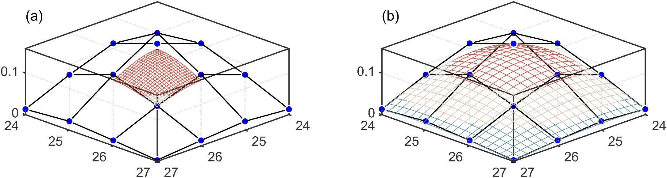
Two categories of B-spline surfaces. Blue dots represent control points, which, together with the black mesh, form the control lattice that defines the B-spline surface. (a) Uniform B-spline surface. (b) Quasi-uniform B-spline surface.
As shown in Figure 2a, the uniform B-spline surface generated by control points does not intersect the control lattice, making it unsuitable for accurate boundary fitting. Therefore, the quasi-uniform B-spline surface is selected to reconstruct the three-dimensional structure of the negative SSAE, as it provides improved boundary adherence. For simplicity, this surface will hereafter be referred to as the “B-spline surface.”
2.4.4 Cross-validation
The shape of the B-spline surface is controlled by the frequencies and . If the frequencies are too low, the model may suffer from underfitting; conversely, excessively high frequencies can lead to overfitting. To balance fitting accuracy and computational efficiency, a 10-fold cross-validation approach (Geisser, 1975; Little et al., 2017) is employed to determine the optimal frequency combination.
In this procedure, the dataset is randomly divided into ten equal parts. Nine parts are used for training, while the remaining part serves as the validation set. The cross-validation is repeated ten times, each time using a different segment as the validation set. The mean absolute error (MAE) computed on the validation sets is used as the evaluation metric to select the frequency combination that achieves the best generalization performance.
2.4.5 Eddy boundary fitting
Under the optimal frequency combination (m-n), the least square method (Ding et al., 2013) is employed to perform B-spline surface fitting. Specifically, the goal is to fit a quasi-uniform bicubic B-spline surface that minimizes the sum of squared errors between the observed data points and the surface approximation. This fitting process is formulated as Equation 9:
The objective of the least squares fitting is to adjust the control point values such that the overall squared deviation between the observed data and the reconstructed surface is minimized. This ensures that the resulting B-spline surface provides the best possible approximation of the three-dimensional eddy-induced sound speed anomaly field under the given frequency configuration.
3 Results
3.1 Extraction of vertical SSA core area
We calculated the SSA at different depths using Equations 1, 2 as described in Section 2. Since the data from each layer contain fewer than 5,000 samples, they are treated as small-sample datasets. To evaluate whether the SSA values follow a normal distribution, the Shapiro–Wilk (S–W) normality test was conducted. The test results are summarized in Table 2.
Table 2
| Depth/m | 0 | 10 | 20 | 30 | 50 | 75 | 100 | 125 | 150 | 200 | 250 | 300 | 400 | 500 |
|---|---|---|---|---|---|---|---|---|---|---|---|---|---|---|
| S-W test | 0.98 | 0.98 | 0.96 | 0.94 | 0.86 | 0.87 | 0.92 | 0.96 | 0.98 | 0.97 | 0.98 | 0.99 | 0.99 | 0.98 |
The result of normality test.
P< 0.05.
At the 5% significance level, all p-values are below 0.05, indicating that the SSA data at various depths deviate from a normal distribution. Consequently, the Spearman correlation coefficient is employed to assess the correlations between water masses at different depths.
Figure 3a illustrates the SSA correlation between water masses at different depths. A distinct stepwise distribution is observed, reflected in the size and color of the polygon. Based on this pattern, the study area can be divided into three vertical zones: 0–30 m, 50–300 m, and below 300 m. Within each zone, water masses exhibit strong positive correlations, while displaying markedly different characteristics compared to those in the other zones.
Figure 3
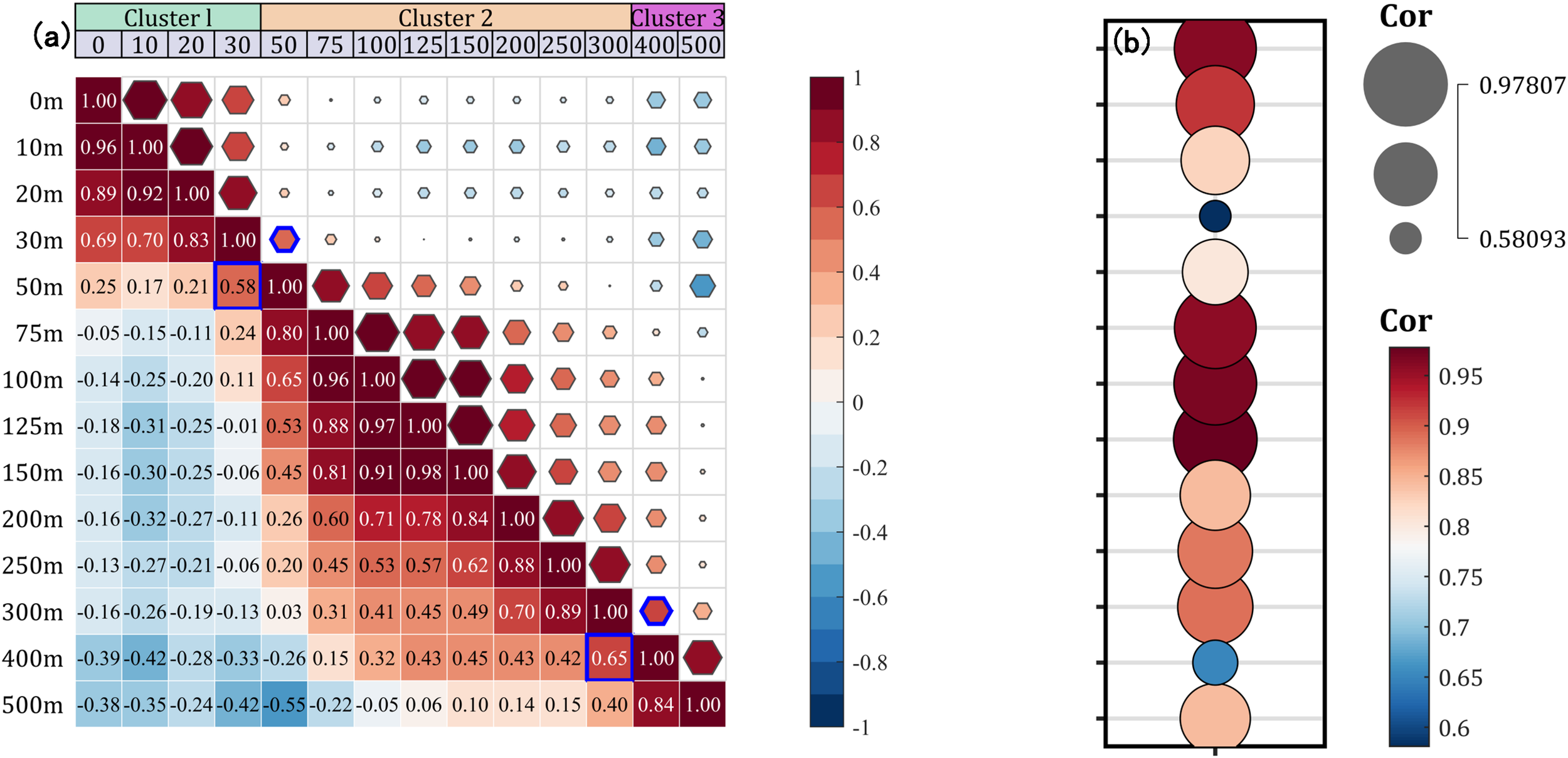
(a) Spearman correlation coefficient of SSA at different depths. The blue polygon highlights the location of two adjacent water masses with the weakest correlation. (b) Correlation strength between adjacent water layers. Larger and darker bubbles indicate stronger correlations between adjacent water masses.
Using the correlation between adjacent water layers as a basis, the vertical SSA core regions can be identified. As shown in Figures 3a, b, two significant drops in correlation occur at depths of 50 m and 300m, indicating shifts in the acoustic characteristics of the water masses between 30–50 m and 300–400 m. Three main factors (Frenger et al., 2015; Zhang et al., 2020) contribute to this phenomenon: Within the upper 0–30 m layer, SSA characteristics remain relatively stable due to the influence of surface factors such as wind. As depth increases, the influence of surface environmental conditions diminishes, and the intrinsic properties of the negative SSA water mass between 50 and 300 m become more evident. Below 300 m, the influence of the negative SSA effect gradually weakens, revealing the original characteristics of the deeper water mass in this region; as a result, the SSA features begin to return to a more moderate state.
Therefore, based on the observed variations in correlation, it can be concluded that the presence of negative SSAE divides the vertical water column into three distinct layers. To minimize the influence of external factors and best preserve the intrinsic characteristics of the negative SSAE, the water mass between 50 and 300 meters is selected for reconstructing the three-dimensional structure of the eddy.
3.2 Extraction of horizontal SSA core area
Following the identification of the vertical SSA core areas, the subsequent key step is to extract the horizontal SSA core areas. As shown in Figure 4, the profile of negative SSAE reveals a distinct vertical core region, outlined by the red dotted line, which is clearly differentiated from the surrounding water masses. In addition, Figure 4a highlights another negative SSA core at 4°E within the eddy structure. The procedure for horizontal core extraction is as follows:
Figure 4
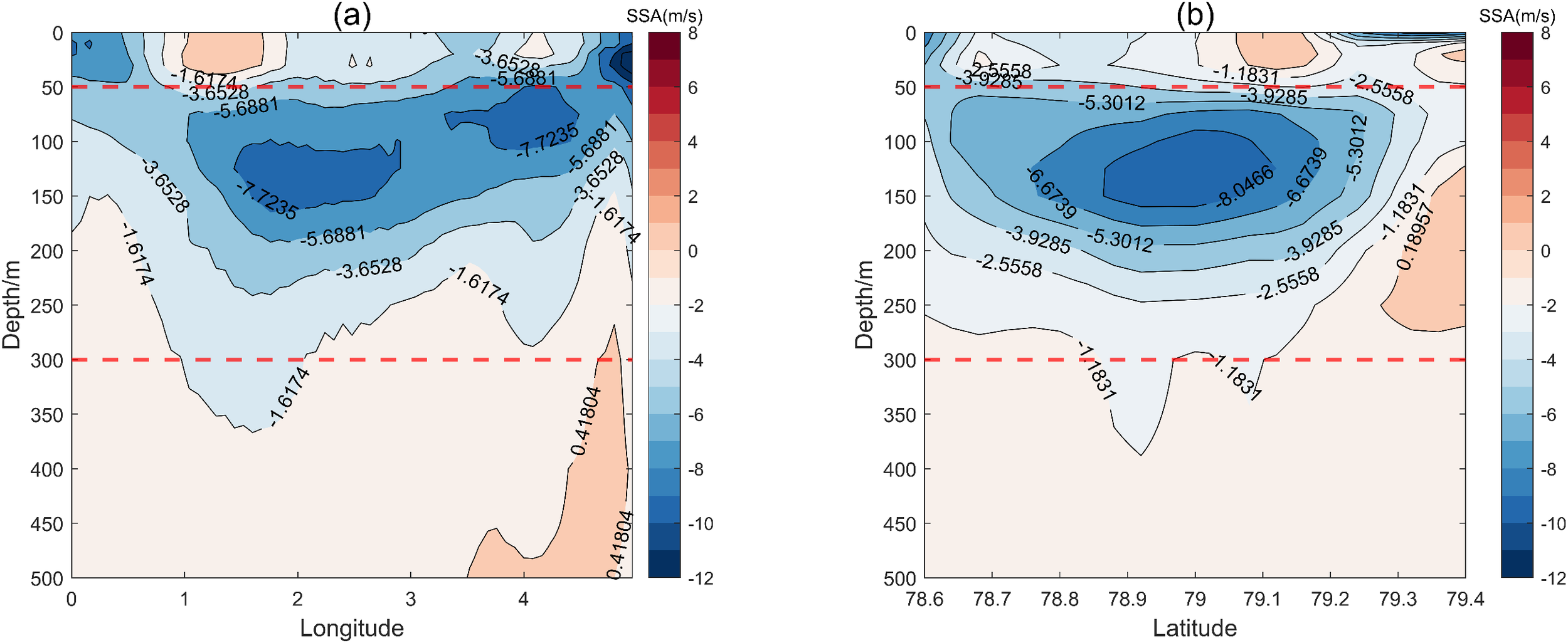
Profile of the negative-SSAE. The region enclosed by the red dotted line represents the vertical SSA core area. (a) Latitude = 78.32: Latitudinal cross-section of the eddy. (b) Longitude = 2.32: Longitudinal cross-section of the eddy.
First, after obtaining SSA data at eight depths—50, 75, 100, 125, 150, 200, and 300 meters—based on the vertical resolution of the HYCOM model, hierarchical clustering is applied to classify the horizontal distribution of different water masses. The clustering results are shown in Figure 5.
Figure 5
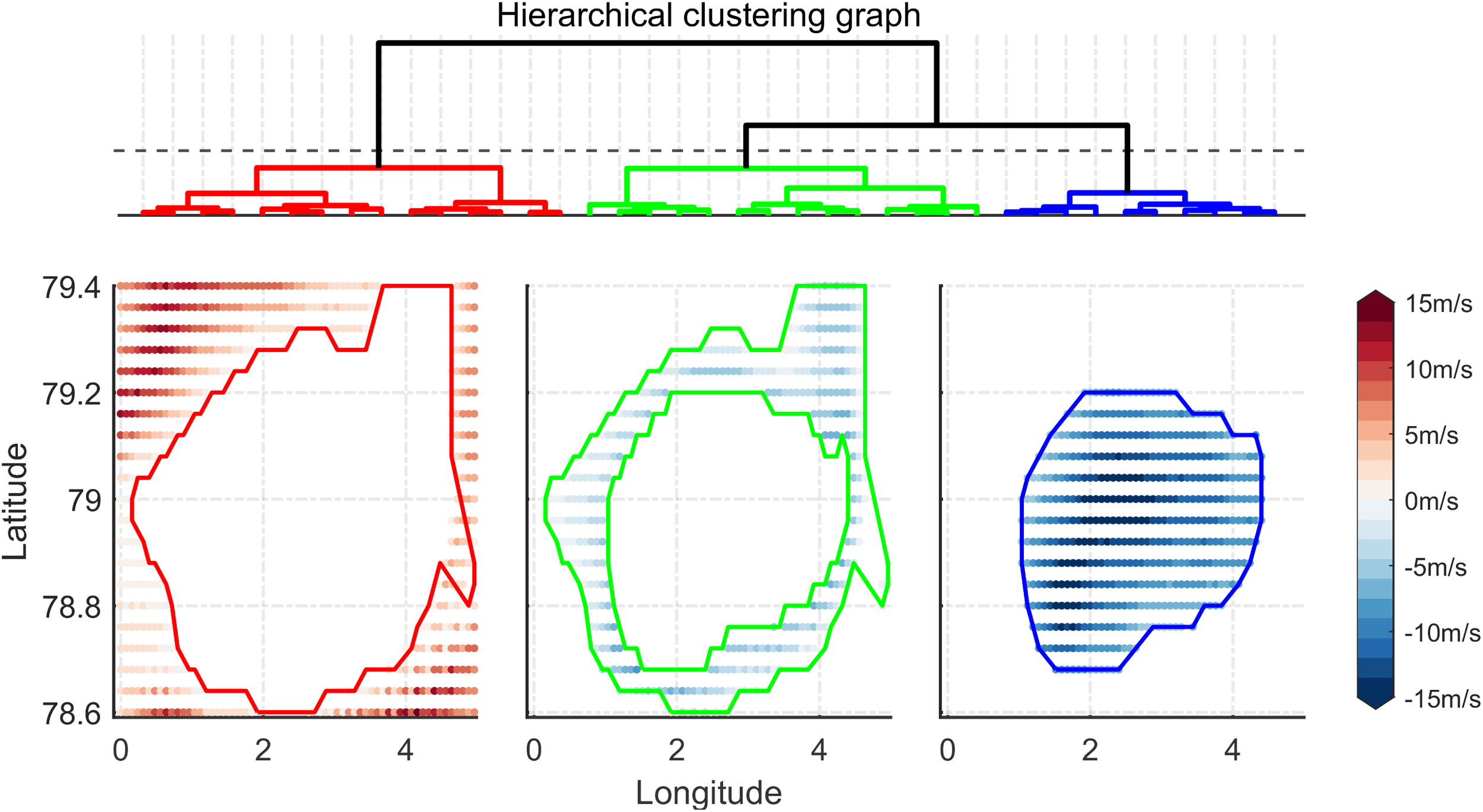
Schematic diagram of hierarchical clustering. The top panel shows the clustering dendrogram, where SSA is divided into three clusters represented by red, green, and blue. The bottom panel displays the spatial distribution of SSA within each cluster.
The SSA at each depth can be categorized into three distinct clusters. The red cluster represents areas with a strong positive SSA, indicating water masses unaffected by the negative SSAE. The green cluster corresponds to the transitional zone between the core influence area and the unaffected regions. The blue cluster denotes the SSA core area in the horizontal direction, capturing the fundamental characteristics of the negative SSAE. To further investigate how the horizontal extent of the SSA core area varies with depth, the results are illustrated in Figure 6.
Figure 6
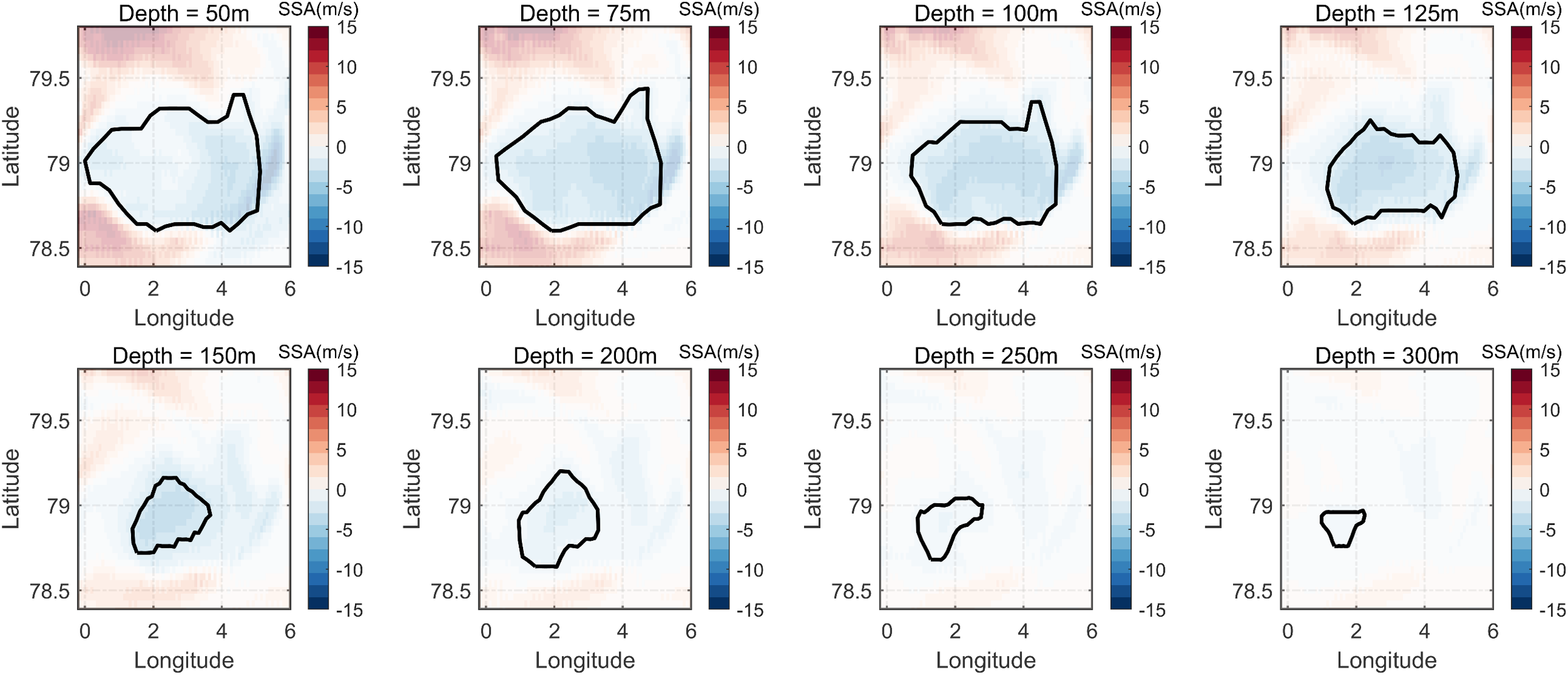
Clustering results of the negative SSAE core area at different depths. The background shows the SSA field, while the black line indicates the boundary of the core area in the horizontal direction.
It can be observed that the SSA core area gradually contracts as depth increases, forming a bowl-shaped structure that slopes southwest. This spatial pattern aligns well with the results (Li et al., 2022), suggesting a consistent three-dimensional manifestation of the negative SSAE. By integrating vertical correlation analysis with horizontal hierarchical clustering, the three-dimensional structure of the SSA core region can be effectively delineated. This combined approach not only captures the vertical layering and horizontal extent of the SSAE, but also establishes a comprehensive framework for accurately identifying and characterizing its complex spatial dynamics.
3.3 The reconstruction of eddy three-dimensional structure
By combining correlation analysis and hierarchical clustering, the three-dimensional distribution of the SSA core area boundary is obtained, as illustrated in Figure 7a. By integrating the boundaries at different depths using B-spline surface fitting, the three-dimensional structure of the negative SSAE can be reconstructed. A critical step in this process is determining the optimal frequency combination in both the longitudinal and latitudinal directions to minimize the fitting error between control points. To achieve this, cross-validation is performed, and the results are presented in Figures 7b, c.
Figure 7
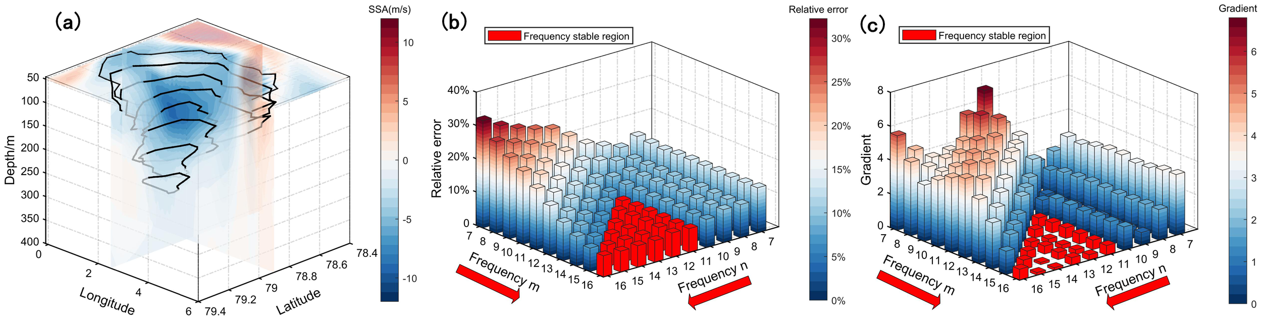
(a) Boundaries of the SSA core area at different depths. The solid black lines indicate the boundaries, while the background shows the SSA field. (b, c) Results of cross-validation: (b) relative error and (c) relative error gradient, represented by height and color, respectively. The red bar highlights the frequency stable region where both error and gradient change smoothly.
As shown in Figure 7b, the relative error decreases steadily with increasing frequencies m and n, indicating a transition from underfitting to a more reasonable fit. However, although higher frequencies are associated with lower relative error, this does not necessarily imply a better fitting effect. In fact, higher frequencies increase the risk of overfitting and require greater computational resources. To determine the optimal frequency, we further calculate the gradient between adjacent relative errors. As shown in Figure 7c, the gradient within the red region remains relatively stable, while the surrounding blue region exhibits significant gradient fluctuations. This indicates that as frequency increases, the B-spline surface fitting undergoes substantial changes at the boundary between the red and blue regions. Beyond this threshold, the relative error shows minimal variation, suggesting diminishing returns in fitting improvement.
Therefore, a frequency-stable region—characterized by smoothly varying error gradients and consistently low relative errors—can be identified, corresponding to the red region shown in Figures 7b, c. All combinations of m and n within this stable region are considered feasible frequencies. However, as frequency increases, the risk of overfitting also rises. Accordingly, the optimal frequency must meet two key criteria:
-
The relative error between the B-spline surface and the original data points (i.e., the SSA core boundaries shown in Figure 7a) should be minimized to ensure high fitting accuracy.
-
The lowest possible frequency values should be used to reduce the risk of overfitting and to optimize computational efficiency.
Based on these criteria, the optimal B-spline surface frequency is determined to be m = n = 11, which yields a relative error of 7.33%, and lies within the frequency-stable region. The resulting B-spline surface fitting is presented in Figure 8:
Figure 8
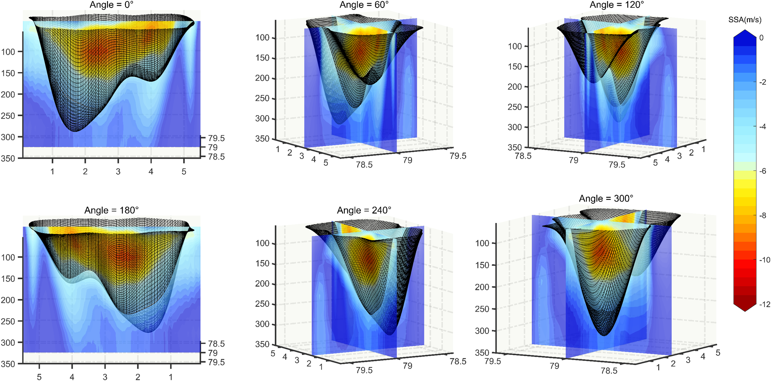
Fitting results of the negative SSAE structure from different viewing angles. The black grid lines represent the fitted mesoscale eddy structure, while the red-blue background slices show the SSA distribution across various cross-sectional profiles.
As illustrated, the B-spline surface provides a reliable representation of the negative SSAE. The reconstructed eddy tilts southwestward with increasing depth, and its boundary encompasses all SSA values greater than 6 m/s (indicated by the yellow to red regions in Figure 8). Additionally, an SSA core region is observed near the 4°E profile, suggesting a possible double-core structure.
4 Discussion
Using hierarchical clustering and B-spline surface fitting, we successfully reconstructed the 3D structure of the negative-SSAE (Figure 8). The reconstruction, based on HYCOM model data, spans depths from 50 m to 300 m. Although the influence of the negative-SSAE extends into the upper 50 m of the ocean, this layer is subject to strong sea surface variability, making its structure highly dynamic and difficult to represent accurately. As a result, we excluded the upper 50 m from our analysis, and the eddy structure within this surface layer can be reasonably approximated by extrapolating the reconstructed eddy structure upward from the 50–300 m depth range.
To quantitatively assess the effectiveness of the reconstruction, we conduct a detailed analysis of key variables—temperature anomaly (TA), salinity anomaly (SA), and sound speed anomaly (SSA)—both inside and outside the reconstructed eddy. The results of this analysis are presented below.
4.1 Differences in the statistical features of the vertical water mass
First, we analyzed the SSA data at different depths. To characterize the central tendency, dispersion, and distribution of the SSA data, we calculated the median, mean, standard deviation, skewness, and kurtosis, thereby obtaining the statistical properties of the SSA at various depths, as shown in Figure 9.
Figure 9
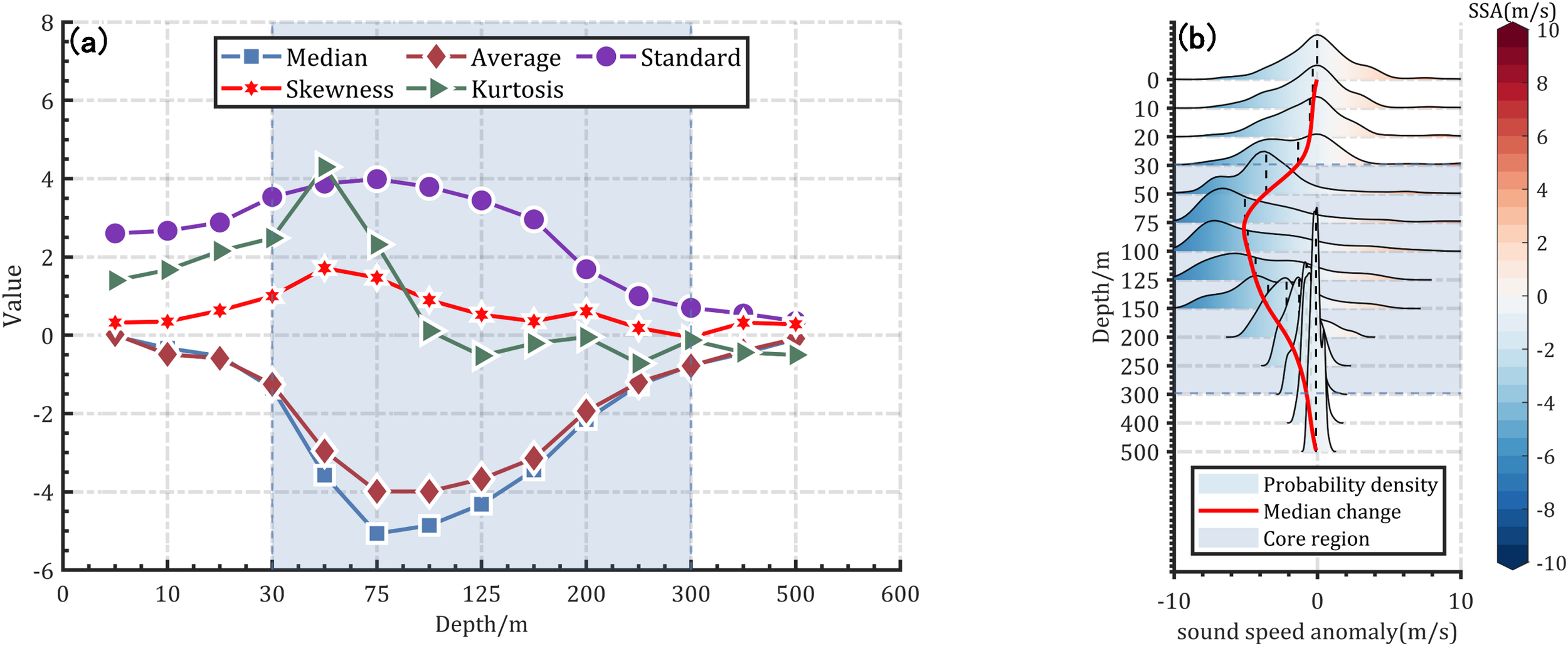
(a) Statistical characteristics of SSA at different depths. From top to bottom along the curve, the purple circles indicate standard deviation, green triangles represent kurtosis, red stars denote skewness, brown diamonds show the mean, and blue squares indicate the median. (b) Histogram of SSA distribution at various depths. The black dashed line represents the median, while the red curve illustrates the overall trend of SSA with depth. The color-filled regions, ranging from blue to red, depict the probability density distribution of SSA. The shaded area highlights the core region that best represents the essential features of the negative-SSAE.
As shown in Figure 9a, the curves of blue squares (median) and brown diamonds (mean) reflect the central tendency of SSA at different depths. Both exhibit a pattern of initially decreasing and then increasing values, particularly within the 50–300 m range. This indicates that the sound speed anomalies at these depths are significantly clustered toward negative values. The green triangles (kurtosis) and red stars (skewness) represent the distribution characteristics of the data, while the purple circles (standard deviation) reflect the degree of dispersion. In contrast to the central tendency, the standard deviation first increases and then decreases, suggesting that the SSA data between 50 m and 300 m are more widely dispersed compared to those in the upper and deeper layers. Furthermore, the non-normality of the distribution—evidenced by higher skewness and kurtosis—is also most pronounced in this depth range. Therefore, based on the statistical characteristics of the SSA data, we conclude that the water masses between 50 m and 300 m differ significantly from those at other depths.
The distribution characteristics of SSA data at different depths are visualized in Figure 9b. At depths shallower than 50 meters and deeper than 300 meters, the data follow an approximately normal distribution. In contrast, betiween 50 m and 300 m, the distribution becomes distinctly skewed, which is consistent with the statistical analysis discussed earlier. Together, the statistical measures and the visualized distribution highlight the existence of a significant negative SSA region within the 50–300 m depth range. This region, associated with the presence of an eddy, leads to substantial alterations in the acoustic properties of the seawater—most notably, a pronounced negative anomaly in sound speed. These observations are in agreement with the SSA correlation patterns between adjacent water masses analyzed in Section 3.
Therefore, the correlation between adjacent water masses can serve as an effective criterion for vertically classifying the eddy structure. This approach is more efficient than analyzing the statistical characteristics and distribution patterns of the eddy at different depths.
4.2 Differences in SSA inside and outside the eddy
An ideally reconstructed eddy structure should divide the region into two water masses with clearly distinct acoustic properties. To assess the effectiveness of the reconstruction in differentiating water masses, we compare the SSA values inside and outside the reconstructed eddy using the Equations 11 and 12:
where refers to a predetermined value representing the SSA at the actual eddy boundary. h1 denotes the proportion of all data points that are smaller than this threshold, while h2 represents the proportion of those below-threshold data points that are located within the eddy.
Since the negative-SSAE is the primary cause of negative SSA in the region, a smaller value of h1 indicates that the threshold more effectively captures the core characteristics of the negative-SSAE. In contrast, a larger h1 suggests that the threshold may encompass additional environmental noise from outside the eddy. Meanwhile, h2 serves as a key indicator of the reconstruction quality: the higher the h2, the more negative SSA data—primarily caused by the negative-SSAE—are encompassed within the B-spline surface, indicating a better fit. Therefore, reconstruction effectiveness can be evaluated in terms of the threshold’s ability to clearly separate water masses with distinct acoustic properties: lower h1 and higher h2 values reflect a more successful reconstruction. Each predetermined threshold corresponds to a specific pair of h1 and h2 values, as shown in Figure 10.
Figure 10
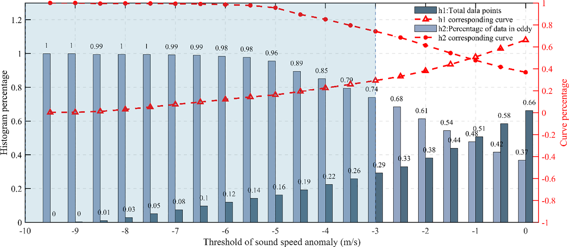
Variation of h1 and h2 values under different predetermined thresholds. The blue-grey bars correspond to the left y-axis and represent the specific values of h1 and h2, while the red dashed curve corresponds to the right y-axis and illustrates the trend of their variation.
At lower thresholds, h1 is small and h2 is large, indicating that the region of negative SSA induced by the eddy—and thus the effective volume of the eddy—is relatively limited. Under these conditions, the reconstructed structure effectively isolates the eddy-induced SSA. As the threshold increases, both the apparent volume of the eddy and the associated SSA range expand. However, this expansion also introduces more environmental noise into the reconstructed structure, diminishing its ability to accurately distinguish the eddy-induced SSA. As a result, h1 increases while h2 decreases, reflecting a decline in the reconstruction’s discriminative capability.
Unlike studies that define the 3D eddy structure based on parameters such as pressure, velocity, or other oceanographic variables, there is currently no established algorithm to determine the optimal SSA value for defining eddy boundaries. Nevertheless, the selection of the threshold plays a critical role in evaluating the accuracy and quality of the reconstructed eddy. In this study, we adopt a threshold of –3 m/s to define the boundary of the negative-SSAE. This corresponds to an h1 value of 29% and an h2 value of 74%, meaning that 29% of the SSA values—including both eddy-induced anomalies and environmental noise—fall below –3 m/s, with 74% of those captured within the reconstructed eddy and the remaining 26% lying outside the eddy boundary. These results indicate that the chosen threshold yields a reasonably accurate and well-fitted reconstruction.
4.3 Differences in temperature/salinity inside and outside the eddy
Although acoustic properties are crucial for identifying different water masses, they are not the sole indicator. To fully evaluate the reconstructed structure, we also analyze temperature and salinity, additional key oceanographic parameters. Their distribution within and outside the reconstructed eddy is shown in Figure 11.
Figure 11
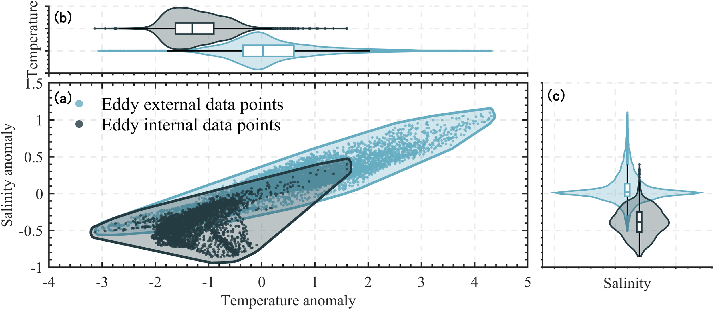
(a) Distribution of temperature and salinity anomaly inside and outside the reconstructed eddy. Black solid lines and dots represent in-eddy data, while blue-green solid lines and dots represent out-of-eddy data. (b) Violin plot showing the distribution of temperature anomalies. (c) Violin plot showing the distribution of salinity anomalies.
As demonstrated, the presence of the negative SSEA leads to significant shifts in the temperature and salinity characteristics within the eddy, resulting in more pronounced negative anomalies and a more concentrated distribution. In contrast, the temperature and salinity outside the eddy exhibit a more symmetrical distribution with a broader range of values. These differences between the interior and exterior of the reconstructed eddy are further illustrated in Figures 11b, c, with the corresponding statistical values summarized in Table 3.
Table 3
| Element | Location | med | uq | lq | Location | med | uq | lq | dmed |
|---|---|---|---|---|---|---|---|---|---|
| Temperature | Outside | 0.1 | 0.6 | -0.4 | Inside | -1.5 | -0.8 | -1.8 | -1.6 |
| Salinity | 0 | 0.2 | -0.1 | -0.3 | -0.3 | -0.6 | -0.3 |
Statistical values of temperature and salinity anomaly.
In Table 3, the parameters med, uq, lq, and dmed represent the median, upper quartile, lower quartile, and the difference in median values (outside median minus inside median), respectively. It is evident that the temperature anomaly quartile range outside the reconstructed eddy decreases from [–0.4, 0.6] to [–1.8, –0.8] inside the eddy, with the median temperature anomaly dropping by 1.6°C. Similarly, the salinity anomaly quartile range narrows from [–0.1, 0.2] to [–0.6, –0.3], accompanied by a median decrease of 0.3. These changes indicate the presence of two distinct water masses with markedly different thermohaline properties inside and outside the reconstructed eddy.
Therefore, the posterior results from the negative-SSAE reconstruction demonstrate significant differences in both acoustic and thermohaline properties between the internal and external water masses, confirming that the reconstructed structure effectively captures the characteristics of the actual eddy and distinguishes it from the surrounding water masses with different properties.
4.4 Fitting surface comparison
Since temperature anomalies at different depths reflect the eddy’s energy transport, and salinity anomalies indicate its mass transport, clustering based on only one element—either temperature or salinity—captures just one aspect of the eddy’s matter-energy dynamics. Therefore, to achieve a more comprehensive analysis that accounts for both mass and energy transport characteristics of the negative-SSAE, we combined temperature and salinity data. We then compared the clustering results from this combined dataset with those based solely on SSA.
Comparing the clustering results in Figure 12, noticeable differences are observed in Figures 12a, g, h between the results based on SSA and those based on temperature-salinity anomalies. However, in Figures 12b–f, the clustering results are generally consistent between the two methods, particularly within the 75–200 m depth range, where the sound speed anomaly is most pronounced. Nevertheless, some discrepancies remain. As highlighted by the yellow box in Figure 12c, while the SSA-based clustering shares similarities with the temperature-salinity-based results, it also exhibits a distinct “peak” structure. The emergence of this unique peak structure can be attributed to at least two factors. First, in the real ocean, the boundary of a mesoscale eddy is rarely smooth or regular. Instead, various sub-mesoscale processes induce irregularities along the eddy edge, creating fine, strip-like structures—reflected in Figure 12 as the “peak” feature—due to the complex dynamics of seawater flow near the eddy boundary. Second, from a data perspective, the distributions of seawater temperature and salinity at 100 m depth, shown in Figures 13a, b respectively, further support these observations.
Figure 12
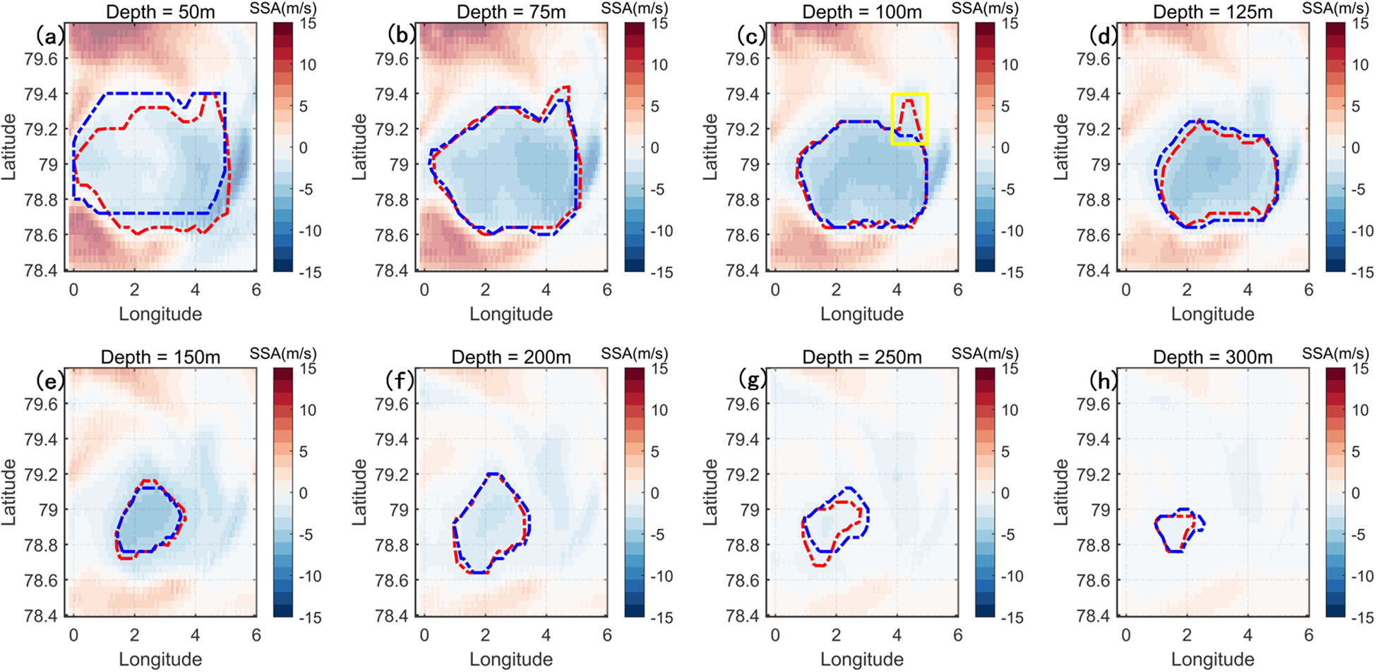
Clustering results based on temperature-salinity anomalies and SSA. (a–h) Clustering outputs at various depths. Blue dotted curves represent clustering based on temperature and salinity, while red dotted curves represent clustering based on SSA. Yellow boxes highlight regions with significant differences between the two clustering methods.
Figure 13
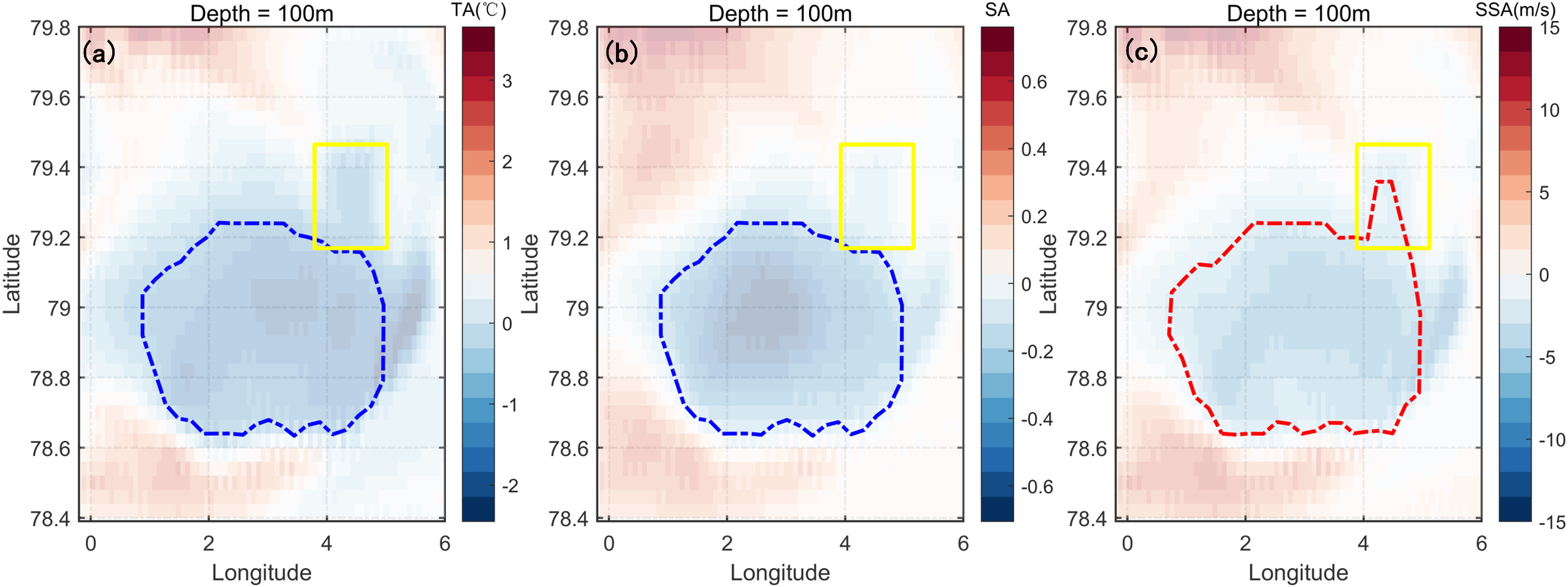
Comparison of clustering results based on different data sources at 100 m depth. The blue dashed line represents clustering based on temperature and salinity; the red dashed line represents clustering based on sound speed anomaly (SSA); the yellow box highlights the location of the “peak” structure. The background of each subfigure shows: (a) temperature anomaly, (b) salinity anomaly, and (c) sound speed anomaly.
As shown in Figure 13a, the sub-mesoscale “peak” structure remains visible in the temperature anomaly field, although it is less pronounced in the salinity anomaly field (Figure 13b). Consequently, when clustering is performed using both temperature and salinity, the weaker salinity signal tends to dilute the sub-mesoscale feature, making the “peak” structure harder to detect. In contrast, while sound speed is derived from both temperature and salinity, its nonlinear formulation (as defined in Equation 1) suppresses the influence of the weaker salinity anomaly and amplifies the more dominant temperature anomaly. As a result, the SSA field (Figure 13c) preserves and even accentuates the “peak” structure, allowing SSA-based clustering to capture sub-mesoscale features more effectively.
Meanwhile, although temperature and salinity respectively represent the energy and mass transport processes of eddies, clustering based on their combination often lacks a clear physical interpretation and remains largely conceptual. Sound speed anomaly, however, possesses explicit physical significance and can be directly measured in practical oceanographic observations. Moreover, as demonstrated in Figure 13, SSA more intuitively reveals sub-mesoscale structures that may be obscured when using temperature-salinity clustering. This highlights SSA as a promising tool for identifying and analyzing sub-mesoscale processes from a fresh perspective.
Therefore, considering the practical measurability of SSA and its enhanced potential ability to reveal sub-mesoscale structures, we recommend using SSA-based clustering rather than temperature-salinity clustering for mesoscale eddy reconstruction.
5 Application
In our study, the three-dimensional structure of the ice-edged eddy and its corresponding 3D edge coordinates are employed to construct a partitioned grid for the eddy-induced three-dimensional sound speed anomaly field in COMSOL Multiphysics, thereby improving the efficiency of underwater acoustic environment simulation.
When considering only the effect of eddies on the underwater acoustic environment, the water outside the eddies tends to remain relatively stable due to minimal eddy influence. In contrast, the water within the eddies exhibits greater variability in acoustic properties due to eddy-induced horizontal trapping and vertical Ekman suction or pumping. As a result, significant differences can arise in the sound speed profile, acoustic propagation direction, and transmission loss (TL) compared to the surrounding waters outside the eddy.
Therefore, when using FEM modeling in COMSOL Multiphysics to compute the underwater acoustic environmental field, different grid densities should be applied inside and outside the eddy. Specifically, since the acoustic environment within the eddy is more unstable, a denser grid is required; conversely, the acoustic environment outside the eddy is relatively stable, allowing for a coarser grid in those regions. Based on this concept, a segment of the ice-edge eddy profile detected by ACOBAR is extracted for the experiment.
As shown in Figure 14a, the eddy boundary—identified using hierarchical clustering and B-spline surface fitting—is indicated by the red line. The sound source and point probe used in the model are represented by the blue square and red dot, respectively. By incorporating local sound speed profile data from HYCOM, a model reflecting the eddy-induced acoustic environment is constructed, as illustrated in Figures 14b, c. In both figures, the left, right, and bottom boundaries are set as Perfectly Matched Layers (PML). The regions inside and outside the eddy are shown in blue and red, respectively. The meshing outside the eddy differs between the two figures: in Figure 14b, the outside mesh is significantly denser with a maximum size of λ/5, whereas in Figure 14c, it is relatively coarser at λ/4. Here, λ denotes the wavelength of the sound wave.
Figure 14
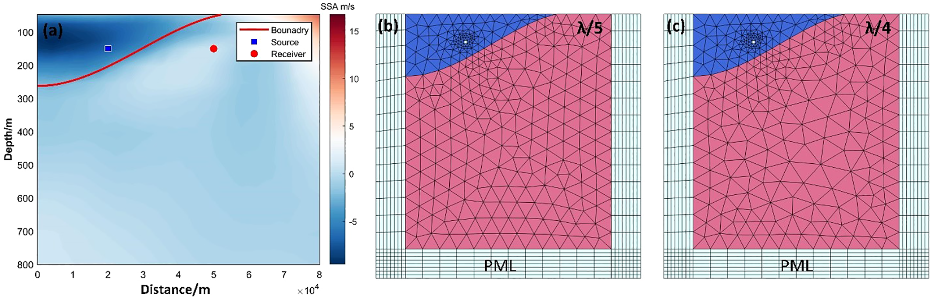
Marine acoustic model construction using FEM in COMSOL Multiphysics. (a) Eddy-induced sound speed anomaly profile observed by ACOBAR. (b, c) FEM-based model construction, where the maximum mesh size outside the eddy is set to (b) λ/5 and (c) λ/4.
Subsequently, the transmission loss of the sound wave is defined as follows:
where and denote the sound intensity at 1 meter and r meters from the source respectively. Based on the Equation 10, the TL at the intercept line along the intercept line between the sound source and point probe is illustrated in Figure 15.
Figure 15

(a) TL at the intercept line. The blue and red lines represent denser and relative sparse outside grids with maximum grid size of λ/5 and λ/4 respectively. Blue and red backgrounds are used to distinguish between the inside and outside regions of the eddy. (b) Probability distribution of TL errors. (c) Accumulated TL error curve.
It can be seen that the TL curves corresponding to the different outside grid densities almost completely overlap, indicating that appropriately reducing the mesh density outside the eddy has little to no effect on the simulation of the eddy-induced underwater acoustic environment. Furthermore, the TL errors and accumulated TL errors for the two different outside grids are presented in Figures 15b, c. The results show that 90% of TL errors are below 3.2 dB, with a mean TL error of 1.2 dB per 20 km, demonstrating good agreement between the TL values obtained using the two grid configurations. To quantitatively illustrate the differences between the two experimental setups, the computational results are summarized as follows:
As shown in Table 4, by maintaining the grid size inside the eddy and reducing the outside eddy grid size from λ/5 to λ/4, the grid construction time decreases by 33.8%. Additionally, the total number of field units, boundary units, and degrees of freedom (DOF) required for the solution are reduced by 33.5%, 13.2%, and 33.4%, respectively, resulting in a 31.7% reduction in overall model computation time. This demonstrates that, in the example presented, applying different grid densities inside and outside the eddy can save over 30% in both computational time and resources, while maintaining a mean TL error of only 1.2 dB per 20 km.
Table 4
| Frequency | Grid(in) | Time | Grid(out) | time | Field unit | Boundary unit | DOF | Computation time |
|---|---|---|---|---|---|---|---|---|
| 100Hz | λ/5 | 79s | λ/5 | 6320s | 34775258 | 111696 | 70101900 | 1950s |
| λ/5 | 79s | λ/4 | 4183s | 23118095 | 96904 | 46681417 | 1332s | |
| Efficiency gain | 33.8% | 33.5% | 13.2% | 33.4% | 31.7% | |||
Comparison of the experiment results.
Therefore, it can be concluded that the proposed method effectively identifies eddy-induced three-dimensional sound speed anomaly fields and facilitates efficient grid construction for marine underwater acoustic environment simulations.
6 Conclusions
In summary, by using sound speed anomalies as indicators for detecting mesoscale eddies, we identify a negative sound speed anomaly associated with an ice-edge eddy on the western side of the Fram Strait, based on sound speed profile data collected by the ACOBAR project. Building on the acoustic property anomalies induced by mesoscale eddies, we propose a novel method that combines sound speed classification with B-spline surface fitting to reconstruct the three-dimensional structure of the ice-edge eddy during the Arctic ice formation period in the Fram Strait. Furthermore, we demonstrate the effectiveness of this method in improving the computational efficiency of marine underwater acoustic environment simulations through finite element modeling using COMSOL Multiphysics.
The implementation of the proposed method consists of the following three main steps:
-
Step 1: Based on the vertical correlation of anomalies between adjacent water masses, extract layers of sound speed anomalies that capture the essential characteristics of the mesoscale eddy.
-
Step 2: Apply an unsupervised learning algorithm to classify the horizontal distribution of sound speed anomalies at different depths into three categories: the non-eddy influence zone, the transition zone, and the eddy core zone.
-
Step 3: Using the three-dimensional sound speed anomaly core region identified in Steps 1 and 2, reconstruct the eddy’s three-dimensional structure by fitting a quasi-uniform B-spline surface.
The results of method validation indicate that the reconstructed eddy structure successfully captures two distinct water masses—inside and outside the eddy—with significantly different temperature, salinity, and acoustic properties. Assuming that all sound speed anomalies below –3 m/s are generated by the ice-edge eddy identified by the ACOBAR project (defining the eddy boundary), the reconstruction achieves an accuracy of 74%. When these reconstructed eddy boundaries are applied to marine underwater acoustic environment simulations, the proposed method reduces computational time and resource consumption by over 30%, while maintaining a mean transmission loss (TL) error of just 1.2 dB per 20 km.
This study demonstrates the effective integration of acoustic sensing, machine learning, and finite element modeling in oceanographic research. It not only deepens our understanding of oceanic eddy structures and their associated acoustic environments but also offers a practical approach for improving the computational efficiency of underwater acoustic simulations. Specifically targeting the challenging polar regions, our research presents a closed-loop workflow for simulating the underwater acoustic environment influenced by individual eddies, encompassing the processes of detection, reconstruction, and simulation. However, as an initial attempt to reconstruct three-dimensional eddy structures from acoustic data, this work has several limitations. Notably, the proposed method relies on field measurements, which are inherently restricted to specific local sea areas. The applicability of our reconstruction approach—combining hierarchical clustering with B-spline surface fitting—to scenarios involving multiple concurrent eddies in the data-scarce polar regions will be further explored in future studies.
Statements
Data availability statement
The original contributions presented in the study are included in the article/supplementary material. Further inquiries can be directed to the corresponding author.
Author contributions
LX: Conceptualization, Data curation, Investigation, Methodology, Project administration, Software, Validation, Visualization, Writing – original draft, Writing – review & editing. JX: Funding acquisition, Resources, Software, Supervision, Validation, Visualization, Writing – review & editing. XZ: Conceptualization, Investigation, Resources, Software, Visualization, Writing – review & editing. AZ: Validation, Visualization, Writing – review & editing. YL: Visualization, Writing – review & editing. DC: Visualization, Writing – review & editing. LC: Visualization, Writing – review & editing. ZW: Visualization, Writing – review & editing.
Funding
The author(s) declare financial support was received for the research and/or publication of this article. This research was jointly supported by (National Natural Science Foundation of China), grant number (41706106).
Acknowledgments
We benefit a lot from discussions with Xianqing Lv from Ocean University of China. We thank the ACOBAR project for making the measured data public.
Conflict of interest
The authors declare that the research was conducted in the absence of any commercial or financial relationships that could be construed as a potential conflict of interest.
Generative AI statement
The author(s) declare that no Generative AI was used in the creation of this manuscript.
Publisher’s note
All claims expressed in this article are solely those of the authors and do not necessarily represent those of their affiliated organizations, or those of the publisher, the editors and the reviewers. Any product that may be evaluated in this article, or claim that may be made by its manufacturer, is not guaranteed or endorsed by the publisher.
References
1
Abert O. Geimer M. Muller S. (2006). Direct and fast ray tracing of NURBS surfaces. Paper presented at 2006 IEEE Symposium Interactive Ray Tracing. 2006, 161–168. doi: 10.1109/RT.2006.280227
2
Amores A. Melnichenko O. Maximenko N. (2017). Coherent mesoscale eddies in the North Atlantic subtropical gyre: 3-D structure and transport with application to the salinity maximum. J. Geophysical Research-Oceans122, 23–41. doi: 10.1002/2016jc012256
3
Ariza A. Lengaigne M. Menkes C. Lebourges-Dhaussy A. Receveur A. Gorgues T. et al . (2022). Global decline of pelagic fauna in a warmer ocean. Nat. Climate Change12, 928–92+. doi: 10.1038/s41558-022-01479-2
4
Boor C. D. (1972). On calculating with B-splines. J. Approximation Theory6, 50–62. doi: 10.1016/0021-9045(72)90080-9
5
Boor C. D. (1978). A practical guide to splines. Appl. Math. Sci.27, 157–157(151). doi: 10.2307/2006241
6
Chelton D. B. Schlax M. G. Samelson R. M. de Szoeke R. A. (2007). Global observations of large oceanic eddies. Geophysical Res. Lett.34. doi: 10.1029/2007gl030812
7
Chen W. Zhang Y. Liu Y. Ma L. Wang H. Ren K. et al . (2022). Parametric model for eddies-induced sound speed anomaly in five active mesoscale eddy regions. J. Geophysical Research C. Oceans: JGR127 (8), e2022JC018408.
8
Cox M. G. (1972). The numerical evaluation of B-splines. IMA J. Appl. Mathematics10(2), 134–149. doi: 10.1093/imamat/10.2.134
9
Cummings J. A. (2005). Operational multivariate ocean data assimilation. Q. J. R. Meteorological Soc.131, 3583–3604. doi: 10.1256/qj.05.105
10
Dalmaijer E. S. Nord C. L. Astle D. E. (2022). Statistical power for cluster analysis. BMC Bioinf.23(1), 205. doi: 10.1186/s12859-022-04675-1
11
de Steur L. Hansen E. Gerdes R. Karcher M. Fahrbach E. Holfort J. (2009). Freshwater fluxes in the East Greenland Current: A decade of observations. Geophysical Res. Lett.36(23). doi: 10.1029/2009gl041278
12
Ding F. Liu X. G. Chu J. (2013). Gradient-based and least-squares-based iterative algorithms for Hammerstein systems using the hierarchical identification principle. Iet Control Theory Appl.7, 176–184. doi: 10.1049/iet-cta.2012.0313
13
Elbanhawi M. Simic M. Jazar R. (2016). Randomized bidirectional B-spline parameterization motion planning. IEEE Trans. Intelligent Transportation Syst.17, 406–419. doi: 10.1109/TITS.2015.2477355
14
Frades I. Matthiesen R. (2010). Overview on techniques in cluster analysis. Methods Mol. Biol. (Clifton N.J.)593, 81–107. doi: 10.1007/978-1-60327-194-3_5
15
Frenger I. Münnich M. Gruber N. Knutti R. (2015). Southern Ocean eddy phenomenology. J. Geophys. Res.: Oceans120, 7413–7449. doi: 10.1002/2015JC011047
16
Geisser S. (1975). The predictive sample reuse method with applications. J. Am. Stat. Assoc.70(350), 320–328.
17
Geyer F. Gopalakrishnan G. Sagen H. Cornuelle B. Challet F. Mazloff M. (2023). Data assimilation of range-and-depth-averaged sound speed from acoustic tomography measurements in Fram Strait. J. Atmospheric Oceanic Technol. 40 (9), 1023–1036. doi: 10.1175/JTECH-D-22-0132.1
18
Geyer F. Sagen H. Cornuelle B. Mazloff M. R. Vazquez H. J. (2020). Using a regional ocean model to understand the structure and variability of acoustic arrivals in Fram Strait. J. Acoustical Soc. America147, 1042–1053. doi: 10.1121/10.0000513
19
Geyer F. Sagen H. Dushaw B. Yamakawa A. Dzieciuch M. Hamre T. (2022). A dataset consisting of a two-year long temperature and sound speed time series from acoustic tomography in Fram Strait. Data Brief42, 108118. doi: 10.1016/j.dib.2022.108118
20
Guan W. T. Chen R. Zhang H. Yang Y. Wei H. (2022). Seasonal surface eddy mixing in the kuroshio extension: estimation and machine learning prediction. J. Geophysical Research-Oceans127(3), e2021JC017967. doi: 10.1029/2021jc017967
21
Hattermann T. Isachsen P. E. von Appen W.-J. Albretsen J. Sundfjord A. (2016). Eddy-driven recirculation of atlantic water in fram strait. Geophysical Res. Lett.43, 3406–3414. doi: 10.1002/2016gl068323
22
Jensen J. K. Hjelmervik K. T. Ostenstad P. (2012). Finding acoustically stable areas through empirical orthogonal function (EOF) classification. IEEE J. Oceanic Eng.37, 103–111. doi: 10.1109/joe.2011.2168669
23
Jensen F. B. Kuperman W. A. Porter M. B. Schmidt H. (2011). Computational Ocean Acoustics (New York, NY: Springer New York).
24
Johannessen O. M. Sagen H. Sandven S. Stark K. V. (2003). Hotspots in ambient noise caused by ice-edge eddies in the Greenland and Barents Seas. IEEE J. Oceanic Eng.28, 212–228. doi: 10.1109/joe.2003.812497
25
Kozlov I. E. Artamonova A. V. Manucharyan G. E. Kubryakov A. A. (2019). Eddies in the western arctic ocean from spaceborne SAR observations over open ocean and marginal ice zones. J. Geophysical Research-Oceans124, 6601–6616. doi: 10.1029/2019jc015113
26
Li H. Xu F. H. Wang G. H. (2022). Global mapping of mesoscale eddy vertical tilt. J. Geophysical Research-Oceans127(11), e2022JC019131. doi: 10.1029/2022jc019131
27
Little M. A. Varoquaux G. Saeb S. Lonini L. Jayaraman A. Mohr D. C. K. et al (2017). Using and understanding cross-validation strategies. Perspectives on Saeb et al. Gigascience6 (5), 1–6. doi: 10.1093/gigascience/gix020
28
Lu C. Xu J. Zhang X. Wang Z. Jin K. (2023). An ocean acoustic modeling based on the physical parameters clustering of the arctic ice floes: applied to the study of acoustic field response as ice floes thickness varies. J. Adv. Modeling Earth Syst.15, e2022MS003188. doi: 10.1029/2022MS003188
29
Murtagh F. Legendre P. (2014). Ward's hierarchical agglomerative clustering method: which algorithms implement ward's criterion? J. Classification31, 274–295. doi: 10.1007/s00357-014-9161-z
30
Nencioli F. Dong C. M. Dickey T. Washburn L. McWilliams J. C. (2010). ). A vector geometry-based eddy detection algorithm and its application to a high-resolution numerical model product and high-frequency radar surface velocities in the southern california bight. J. Atmospheric Oceanic Technol.27, 564–579. doi: 10.1175/2009jtecho725.1
31
Pnyushkov A. Polyakov I. V. Padman L. Nguyen A. T. (2018). Structure and dynamics of mesoscale eddies over the Laptev Sea continental slope in the Arctic Ocean. Ocean Sci.14, 1329–1347. doi: 10.5194/os-14-1329-2018
32
Rudels B. Friedrich H. J. Quadfasel D. (1999). The arctic circumpolar boundary current. Deep-Sea Res. Part Ii-Topical Stud. Oceanography46, 1023–1062. doi: 10.1016/s0967-0645(99)00015-6
33
Sandalyuk N. V. Bosse A. Belonenko T. V. (2020). The 3-D structure of mesoscale eddies in the lofoten basin of the norwegian sea: A composite analysis from altimetry and in situ data. J. Geophysical Research-Oceans125 (10), e2020JC016331. doi: 10.1029/2020jc016331
34
Schober P. Boer C. Schwarte L. A. (2018). Correlation coefficients: appropriate use and interpretation. Anesth. Analgesia126, 1763–1768. doi: 10.1213/ane.0000000000002864
35
Schourup-Kristensen V. Wekerle C. Danilov S. Volker C. (2021). Seasonality of mesoscale phytoplankton control in eastern fram strait. J. Geophysical Research-Oceans126 (10), e2021JC017279. doi: 10.1029/2021jc017279
36
Shuchman R. A. Burns B. A. Johannessen O. M. Josberger E. G. Campbell W. J. Manley T. O. et al . (1987). Remote sensing of the fram strait marginal ice zone. Sci. (New York N.Y.)236, 429–431. doi: 10.1126/science.236.4800.429
37
Storheim E. Sagen H. Geyer F. (2021). Analysis of signal propagation in the UNDER-ICE experiment. Proc. Meetings Acoustics44(1), 070031. doi: 10.1121/2.0001500
38
Tang H. S. Feng Z. X. Cheng D. W. Wang Y. T. (2023). Parallel ray tracing through freeform lenses with NURBS surfaces. Chin. Optics Lett.21(5), 052201. doi: 10.3788/col202321.052201
39
Timmermans M. L. Marshall J. (2020). Understanding arctic ocean circulation: A review of ocean dynamics in a changing climate. J. Geophysical Research-Oceans125 (4), e2018JC014378. doi: 10.1029/2018jc014378
40
van Eck N. J. Waltman L. (2017). Citation-based clustering of publications using CitNetExplorer and VOSviewer. Scientometrics111, 1053–1070. doi: 10.1007/s11192-017-2300-7
41
Wang Z. C. Xu J. Zhang X. F. Lu C. Jin K. K. Zhang Y. Q. (2021). Flow-dependent modeling of acoustic propagation based on the DG-FEM method. J. Atmospheric Oceanic Technol.38, 1823–1832. doi: 10.1175/jtech-d-21-0001.1
42
Xu L. C. A. Gao M. Zhang Y. R. Guo J. T. Lv X. Q. Zhang A. M. (2022). Oceanic mesoscale eddies identification using B-spline surface fitting model based on along-track SLA data. Remote Sens.14(22), 5713. doi: 10.3390/rs14225713
43
Yuan Y. P. Castelao R. M. (2017). Eddy-induced sea surface temperature gradients in Eastern Boundary Current Systems. J. Geophysical Research-Oceans122, 4791–4801. doi: 10.1002/2017jc012735
44
Yuan L. M. Tian F. L. Xu S. Q. Zhou C. Chen J. (2021). Three-dimensional mesoscale eddy identification and tracking algorithm based on pressure anomalies. J. Oceanology Limnology39, 2153–2166. doi: 10.1007/s00343-021-0309-5
45
Zhang Z. G. Wang W. Qiu B. (2014). Oceanic mass transport by mesoscale eddies. Science345, 322–324. doi: 10.1126/science.1252418
46
Zhang Y. Wang N. Zhou L. Liu K. Wang H. (2020). The surface and three-dimensional characteristics of mesoscale eddies:A review. Advance Earth Sci.35, 568–580. doi: 10.11867/J.ISSN.1001-8166.2020.050
47
Zhang Z. G. Zhang Y. Wang W. Huang R. X. (2013). Universal structure of mesoscale eddies in the ocean. Geophysical Res. Lett.40, 3677–3681. doi: 10.1002/grl.50736
48
Zhao D. Xu Y. Zhang X. Huang C. (2021). Global chlorophyll distribution induced by mesoscale eddies. Remote Sens. Environ.254, 112245. doi: 10.1016/j.rse.2020.112245
Summary
Keywords
oceanic eddies, machine learning, B-spline surface, underwater acoustic field, finite element method
Citation
Xu L, Xu J, Zhang X, Zhang A, Liu Y, Chen D, Chen L and Wu Z (2025) Eddy-induced underwater acoustic field reconstruction and computation based on sound speed classification and B-spline surface fitting. Front. Mar. Sci. 12:1583080. doi: 10.3389/fmars.2025.1583080
Received
25 February 2025
Accepted
21 July 2025
Published
12 August 2025
Volume
12 - 2025
Edited by
Andrea Storto, National Research Council (CNR), Italy
Reviewed by
Chengbo Wang, University of Science and Technology of China, China
Rongbin Lin, Shenzhen Research institute of Xiamen University, China
Updates
Copyright
© 2025 Xu, Xu, Zhang, Zhang, Liu, Chen, Chen and Wu.
This is an open-access article distributed under the terms of the Creative Commons Attribution License (CC BY). The use, distribution or reproduction in other forums is permitted, provided the original author(s) and the copyright owner(s) are credited and that the original publication in this journal is cited, in accordance with accepted academic practice. No use, distribution or reproduction is permitted which does not comply with these terms.
*Correspondence: Xuegang Zhang, 16608816416@163.com
Disclaimer
All claims expressed in this article are solely those of the authors and do not necessarily represent those of their affiliated organizations, or those of the publisher, the editors and the reviewers. Any product that may be evaluated in this article or claim that may be made by its manufacturer is not guaranteed or endorsed by the publisher.