Predicting Pacific saury fishing sites using machine learning and spatial environmental variables reflecting recent eastward shifts

In recent years, the Northwest Pacific has seen a decline in Pacific saury (Cololabis saira) catch and an eastward shift of fishing grounds, both of which have posed increasing challenges for effective resource management. To identify environmental drivers underlying the formation of Pacific saury fishing grounds, we developed machine learning-based prediction models using spatial environmental variables. Our models combined fishing site and pseudo-absence data with high-resolution oceanographic data from the Japan Fisheries Research and Education Agency Regional Ocean Modeling System (FRA-ROMS). We employed three machine learning methods to evaluate three types of explanatory variable representations: averaged, vectorized, and spatially structured. The results demonstrated that preserving spatial structure using a two-dimensional grid layout improved model performance. Our prediction results reflected the recent eastward shifting fishing grounds, suggesting a strong influence of environmental factors, particularly water temperature derived from the ocean circulation model. The convolutional neural network model, which best replicated the eastward shift of fishing sites, achieved a recall of 45.0% and a precision of 95.4%, although its performance declined under higher environmental novelty, which was associated with low-catch years (2020-2022). By evaluating how different spatial representations of environmental variables affect model performance, this study demonstrates that incorporating spatial structure improves predictive ability and enables models to capture recent eastward shifts in fishing activity under changing ocean conditions.

1 Introduction

Pacific saury (Cololabis saira) is one of the most commercially significant pelagic fish species in the North Pacific Ocean. It is primarily caught in Japan, Russia, South Korea, China, Taiwan, and Vanuatu (Hubbs, 1980; Suyama et al., 2006; Fuji et al., 2021). This fishery is crucial for these countries’ economies, especially in Japan where saury is a culturally important seasonal food. Therefore, any considerable changes in its abundance or spatial distribution may impact the economy. Pacific saury landings in Japan exceeded 200,000 tons in 2013 but dropped below 20,000 tons in 2022, indicating a sharp decline in stock availability and economic value. Detailed fluctuations in catch are reported in the annual stock assessment reports by the North Pacific Fisheries Commission (NPFC, 2024). Pacific saury, with a lifespan of 2 years, migrate long distances across the North Pacific Ocean, and their distribution is heavily influenced by ocean currents and conditions (Suyama et al., 2006). Several studies have reported that the distribution and recruitment of Pacific saury are strongly influenced by oceanographic features such as temperature fronts and surface currents, and that catch-per-unit-effort (CPUE) has declined in association with these environmental changes (Tseng et al., 2013, 2014; Ichii et al., 2018; Huang et al., 2019; Yatsu et al., 2021).

The oceanographic factors, such as sea surface temperature and height, is closely related to the movement patterns and habitat selection of Pacific saury (Pittman and Brown, 2011; Yasuda et al., 2014; Kakehi et al., 2020). The Oyashio–Kuroshio frontal zone is an area with increased eddy activity and where water masses of different origins converge, creating an environment that is rich in food for Pacific saury (Prants et al., 2020). Moreover, the larvae’s location and the plankton that Pacific saury feed on are also affected by ocean currents (Tian et al., 2003; Ito et al., 2004; Baitaliuk et al., 2013). Recent observations also highlight the influence of variations in the Kuroshio’s pathway, particularly the persistent “large meander” state that has continued since 2017. These changes have altered regional ocean conditions, including sea surface temperatures, eddy fields, and fishery distributions (Hirata et al., 2025).

The location of Pacific saury fishing grounds has significantly shifted eastward in recent years (Miyamoto et al., 2019; Suyama et al., 2019; Kakehi et al., 2020). Biomass estimates suggest an eastward shift in the center of distribution since 2010 (Hashimoto et al., 2020). This shift in fishing sites will escalate travel time for vessels, thereby increasing the fuel consumption and operating costs of fishing vessels. Hence, predicting fishing sites and gaining insight into the stock fluctuations for this species based on ocean conditions will meaningfully contribute from economic and resource management perspectives. While many previous studies have employed habitat models to estimate fishing site suitability, few have investigated this long-term directional shift using high-resolution spatial data (Kakehi et al., 2020; Xing et al., 2022). Recent models have begun to incorporate mesoscale oceanographic features, yet high-resolution approaches remain rarely applied to Pacific saury. Consequently, conventional methods may struggle to predict saury distributions under changing conditions (Xing et al., 2022). In addition, while numerous studies have developed models using point-based data at individual fishing locations (Liu et al., 2022; Xing et al., 2022), limited research has examined how different input designs and spatial configurations influence prediction performance.

Here, we combined fishing site and pseudo-absence data with a high-resolution regional ocean model (FRA ROMS) to incorporate spatially continuous environmental information and examine the distribution of Pacific saury under changing oceanographic conditions. The methods used to predict fishing sites were random forest (RF) and convolutional neural network (CNN), both of which are widely used machine learning algorithms. These methods were selected for their ability to effectively capture nonlinear relationships and complex spatial patterns in environmental data, which are commonly observed in fisheries studies (Glaser et al., 2014; Han et al., 2023). Moreover, compared to conventional species distribution models (SDMs), such as generalized linear models (GLMs), machine learning provides greater flexibility and enhanced predictive performance, making it a powerful tool for modeling complex ecological systems (Gobeyn et al., 2019; Liu et al., 2024). Modeling forage species like Pacific saury is particularly difficult because they are highly mobile and respond to short-term environmental changes across broad spatial scales. This study addresses these challenges by applying machine learning models that incorporate spatially structured environmental data. The overall modeling framework is illustrated in a conceptual diagram (Figure 1), where environmental variables were extracted as a spatial range centered around each fishing location. Furthermore, to our knowledge, no existing models have successfully replicated the long-term eastward shift of Pacific saury using historical data, despite its critical importance for understanding stock availability and climate-driven distributional changes. This study provides a novel approach to tackle this challenge by combining ocean reanalysis products with spatially aware machine learning, offering new insights for ecosystem-based fisheries management.

Figure 1

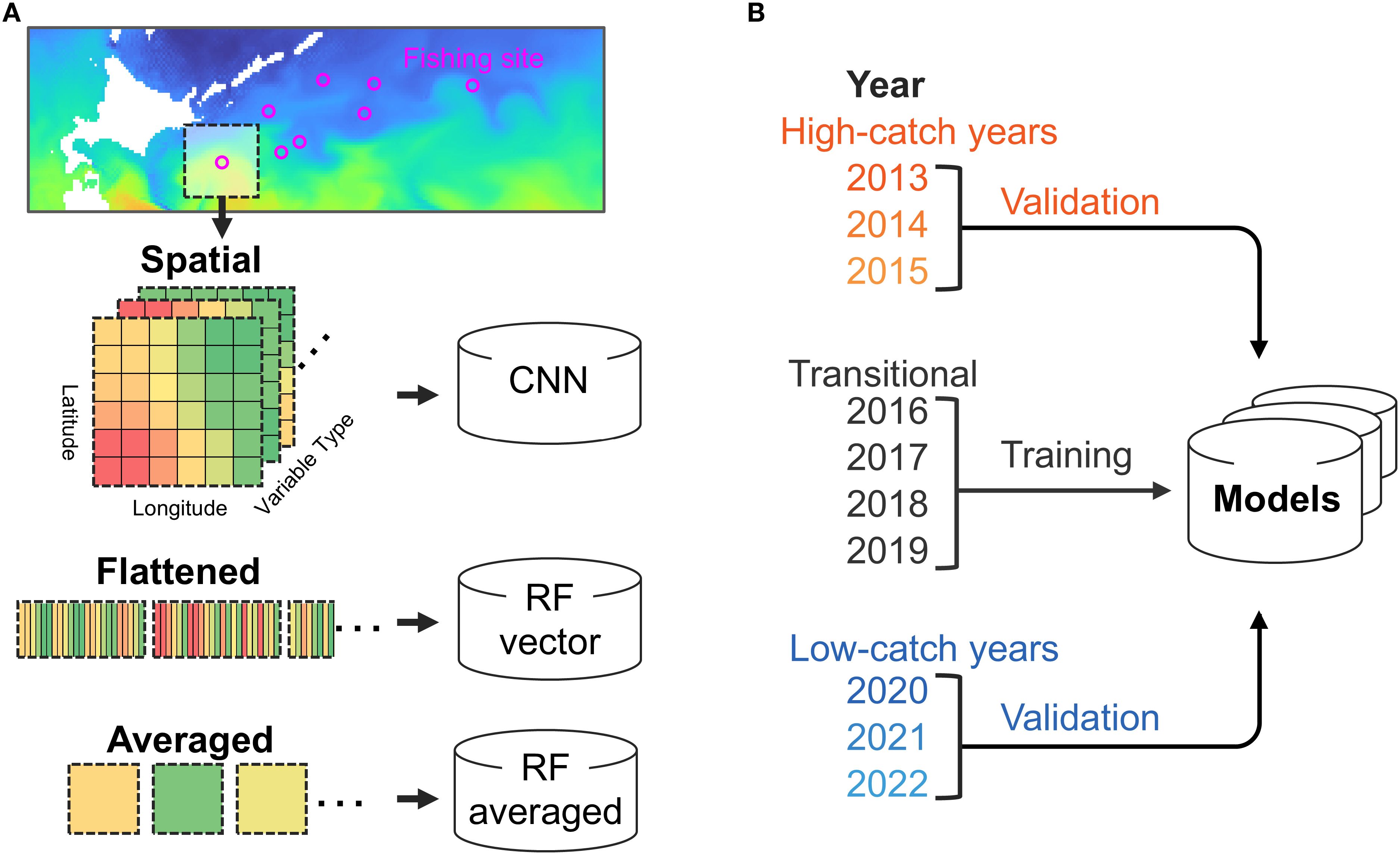
Figure 1. Overview of variable acquisition and validation settings. (A) Method for obtaining explanatory variables in a predictive model and the models used. (B) The years designated for model training and the year designated for validation.

2 Materials and methods

2.1 Pacific saury data

The Pacific saury fishing position in latitude and longitude for the period from 2013 to 2022, sourced from the Fisheries Agency, corresponded to the date and location of the catch (Figure 2). We used fishing records from Japanese commercial stick-held dip net fisheries targeting Pacific saury. A “fishing site” was defined as the precise location where fishing activity occurred, based on recorded latitude and longitude.

Figure 2

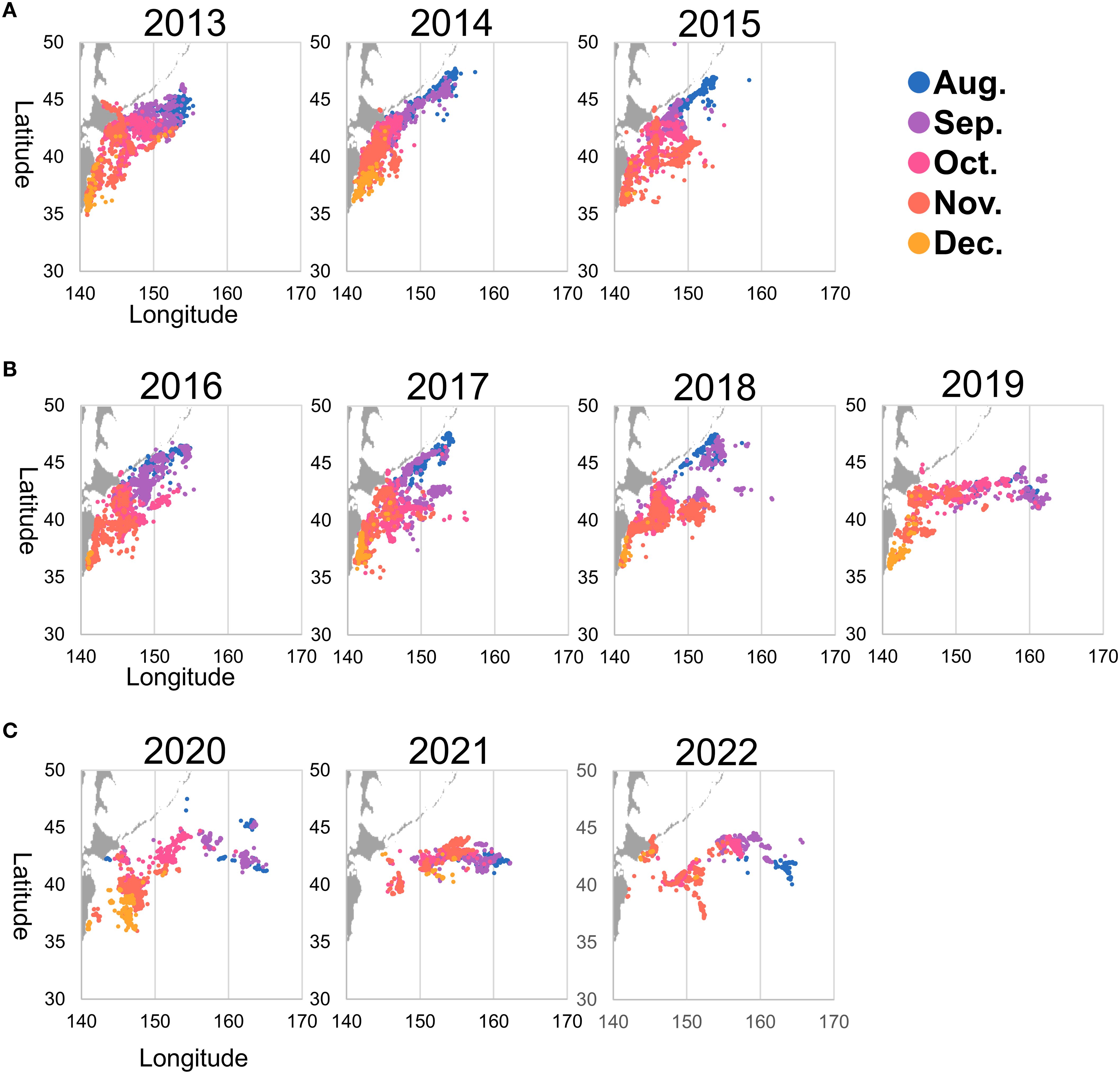
Figure 2. Pacific saury fishing locations (2013–2022) with points color-coded by month. The figure illustrates seasonal patterns and interannual changes, such as an eastward shift in fishing grounds. (A) represents a high-catch year, (B) corresponds to the model training period, and (C) represents a low-catch year.

These records covered the main fishing season, which extends from August to December each year. The data included the geographic locations of fishing operations across a broad region of the northwestern Pacific, ranging from 35°N to 50°N in latitude and from 140°E to 170°E in longitude. The response variable was the fishing or nonfishing status of Pacific saury catches. Locations where catches occurred were assigned a value of “1.0”. However, there was very little data available for locations where no catch occurred. To address this, pseudo-absence data were generated by randomly sampling dates, latitudes, and longitudes from the fishing grounds, and assigning a value of “0.0” to these sampled points. The number of these pseudo-absence entries was matched to the number of “1.0” entries. Finally, the date and location information for both “1.0” and “0.0” points were combined to create a dataset indicating the presence or pseudo-absence of catches at specific times and places.

2.2 Environmental data

The environmental information used as explanatory variables for learning and prediction included temperature, SSH, and ocean current velocity reanalyzed by FRA-ROMS II. This ocean data assimilation system estimates reanalyzed products by combining observation and simulation data for the waters around Japan (Fujii and Kamachi, 2003; Kuroda et al., 2017). The data resolution provided by FRA-ROMS is 0.1° × 0.1° per grid cell. In line with the Pacific saury fishing range and season, the target season was Aug. 1st to Dec. 31st in 140°E–180°E and 30°N–50°N. Daily water temperature (depths: 0, 30, 50 m, unit: °C), sea surface height (depth: 0 m, unit: m), and ocean current velocity (depth: 0 m, unit: m/s, including both east–west (u) and north–south (v) components) were obtained for 2013 to 2022. Each data was obtained in a numerical data structure corresponding to latitude and longitude, with six variables per grid cell. Environmental variables were extracted from square grid regions of variable size centered on each fishing site or pseudo-absence location, using data from FRA-ROMS. This design allowed the models to learn localized oceanographic conditions associated with fishing activity.

The temporal resolution of the environmental data was daily, and the values used for each sample corresponded to the same date as the fishing sites or pseudo-absences entry. Some nearshore fishing sites included land areas within the extracted environmental range, resulting in missing values. To ensure compatibility with machine learning algorithms that cannot process missing data, these were replaced with randomly selected values within the valid range for each variable.

2.3 Models

In this study, we constructed three learning models based on two machine learning approaches: RF and CNN (Figure 1A and Table 1). Among the three models, two were constructed using the RF algorithm, while the other one was based on CNN architecture. RF, an ensemble classifier, generates and combines multiple decision trees using randomly selected samples and variables (Breiman, 2001). Its high accuracy and noise robustness make it suitable for predicting trends in marine fishing (Belgiu and Drăguţ, 2016; Stock et al., 2020; Behivoke et al., 2021). CNN, the most frequently used deep learning technique for spatial pattern analysis, learns spatial features by convolving data. Its grid cell-based data arrangement makes it an ideal tool for processing remote sensing and ocean model data (LeCun et al., 1989, 2015; Han et al., 2023). Unlike traditional statistical models such as generalized linear models (GLMs), RF and CNN are non-parametric methods that do not require predefined link functions or distribution families, making them more flexible for modeling complex ecological patterns. We selected these two approaches to compare differences in input data structures while keeping the model comparison conceptually simple. RF was also chosen because it requires fewer hyperparameters than other tree-based methods, facilitating a more straightforward comparison.

Table 1

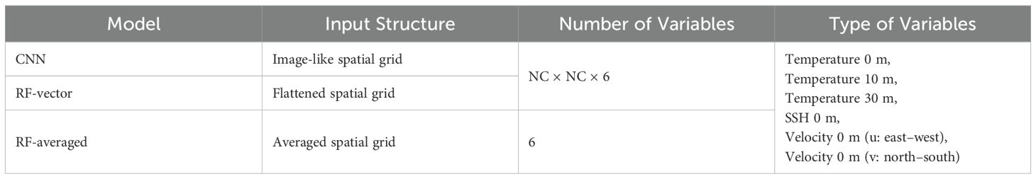
Table 1. Summary of explanatory variable configurations for each model.

The first model was a random forest model (RF-averaged) in which environmental variables from all grid cells within the square region centered on each fishing or nonfishing site were averaged into a single value. Each square had a size of NC × NC grid cells, where NC is the number of grid cells on one side of the square. To determine the optimal value of NC, we tested four spatial ranges (NC = 16, 24, 32, 40, 48, 56 and 64) and evaluated model performance for each setting. Based on validation results, the most accurate configuration was selected and consistently applied across models. The number of decision trees was set to 100, which is generally sufficient to stabilize prediction performance in cases with a limited number of input features. The max_features parameter, which controls the number of features considered at each split, was set to 6 because this corresponds to the total number of input variables, and with few explanatory variables, random feature selection would not improve performance.

The second model was a random forest (RF-vector) that used environmental variables extracted from a square area around each site, which were flattened into a one-dimensional vector for input. The total number of explanatory variables was NC × NC × 6. The key input variables, such as temperature and SSH, exhibit temporal and spatial autocorrelation because of their geophysical nature, with particularly strong correlation observed among adjacent cells. While RF models are relatively robust to high-dimensional input owing to their ensemble nature, there remains a potential risk of overfitting, particularly due to redundant variables. In this study, to ensure fair comparison across models, we deliberately accepted this risk and did not apply explicit variable selection. The number of features to use in the decision tree was set to the square root of the total number of variables, and the number of decision trees was set to 1,000. Although the value was not rigorously optimized, the number of decision trees in the RF models was set to a sufficiently large value to ensure that all variables contribute to the analysis.

The third model employs a CNN. Similar to RF-vector, explanatory variables were obtained in a square centered on the “fishing sites or pseudo-absences; however, unlike RF-vector, the CNN model retained the spatial structure of the input grid. The model was constructed with a sequential architecture with the following configuration: 1. The input layer used a (3, 3) convolutional layer with 128 filters, applied the ReLU activation function and batch normalization, and inserted a (2, 2) pooling layer. 2. Four additional convolutional layers were similarly built with 112, 64, 64, and 128 filters. 3. After the last convolutional layer, a (2, 2) pooling layer and a dropout layer (dropout rate 0.2) were inserted (Supplementary Figure S1).

The analysis was performed using Python (3.9.7), with Sci-kit Learn (1.3.2) for random forests and Keras and TensorFlow (2.6.0) libraries for CNNs. Please refer to the Supplementary Script Files (Supplementary_Scripts.docx) for more details on the models. The script files used in the analysis are provided as Supplementary Materials.

2.4 Validation

The machine learning models were trained using data for 19,326 fishing sites collected from Japanese fishing vessels between 2016 and 2019. To evaluate the temporal generalization ability of the models, their accuracy was assessed using fishing data from independent years preceding and following the training period: 2013, 2014, 2015, 2020, 2021, and 2022 (Figure 1B and Supplementary Figure S2). Since 2013, the catches of Pacific saury have shown a clear declining trend, with the 2022 catch being the lowest ever recorded (Supplementary Figure S2). In parallel with this trend, the number of fishing sites has also consistently decreased, accompanied by a gradual eastward shift in their locations (Figure 2). Therefore, when setting the training and validation data, common validation methods that switch the training and validation data, such as the leave-one-out and k-fold methods, could change the quality and quantity of the training data for each validation. To validate the recent changes in Pacific saury, such as the eastward shift, using a model trained on consistent learning data, the training period was fixed from 2016 to 2019, and predictions and validation were performed 3 years before and after. In this study, such years were referred to as “high-catch years” (2013–2015) and “low-catch years” (2020–2022) based on the total catch volume, because of the remarkable fluctuations in catch volumes between the three preceding and following years (Figure 2).

Although the COVID-19 pandemic may have influenced fisheries operations to some extent, its impact on total catch volume, which serves as the basis for classifying years into “high-catch” and “low-catch” categories, is considered minor. This is supported by the fact that the decline in Pacific saury catch had already begun well before 2020, indicating a longer-term downward trend independent of the pandemic (Supplementary Figure S2). The models were evaluated by comparing prediction results against these catch locations. In comparing recall and precision metrics across various conditions and models, true fishing sites were defined as the specific locations where fishing activity occurred on a given day, based on recorded latitude and longitude data. Due to the spatial resolution of the FRA-ROMS dataset (0.1° × 0.1°), these points were matched to the corresponding grid cell. Sites with predicted values of 0.5 or higher were considered true positive (TP), otherwise false negative (FN). The recall rate (TP/(TP + FN)) was calculated as the proportion of fishing sites correctly predicted each year. Additionally, a predicted value of 0.5 or higher for a randomly generated point was considered a false-positive (FP), and precision was calculated as (TP/(TP + FP)). Precision was used instead of specificity because it better reflects the reliability of predicted fishing sites, which is more relevant for evaluating the usefulness of the model in identifying productive fishing grounds. To assess the relative importance of each environmental variable, we conducted a jackknife analysis by systematically removing one variable at a time from the model inputs and evaluating the resulting change in prediction performance. Variables whose exclusion led to a substantial decrease in model accuracy were considered more influential in the model. For water temperature, which was available at three depths (0, 10, and 30 m), we tested both individual layer exclusion and the removal of all layers together. For ocean current velocity, the east–west (u) and north–south (v) components were excluded as a pair.

2.5 Environmental novelty calculation

Environmental Novelty Calculation To assess environmental novelty, we calculated the Mahalanobis distance between environmental conditions in the validation years and those in the training period (2016–2019). For each fishing site, environmental variables were averaged within a square range centered on the point. Mahalanobis distance was computed between years for each month, using the mean vector and covariance matrix of the environmental variables from the training period as the reference. Mahalanobis distance provides a measure of how distinct a given environmental condition is from the training baseline, with higher values indicating greater environmental novelty.

3 Results

Overall, the CNN and RF-vector models showed the best overall performance, accurately reproducing both the seasonal westward movements and the interannual eastward shift of fishing grounds. Notably, the CNN model best captured the eastward shift observed since 2020. In contrast, the RF-averaged model performed less well, especially in spatial prediction accuracy. Interannual differences in model performance were also evident, with generally lower accuracy during low-catch years.

Among the three models, RF-vector showed the highest recall and CNN showed the highest precision across the six validation years (Figure 3). Recall and precision were comparable between CNN and RF-vector models, while RF-averaged showed noticeably lower precision. For detailed validation results across models and years, see Supplementary Table S1. For both models, although the recall rate improved as the range increased, the precision reached its peak at 40-grid cells. The annual recall and precision calculations for 40-grid cells are displayed in Figure 3B. Recall and precision demonstrated a decrease in low-catch years.

Figure 3

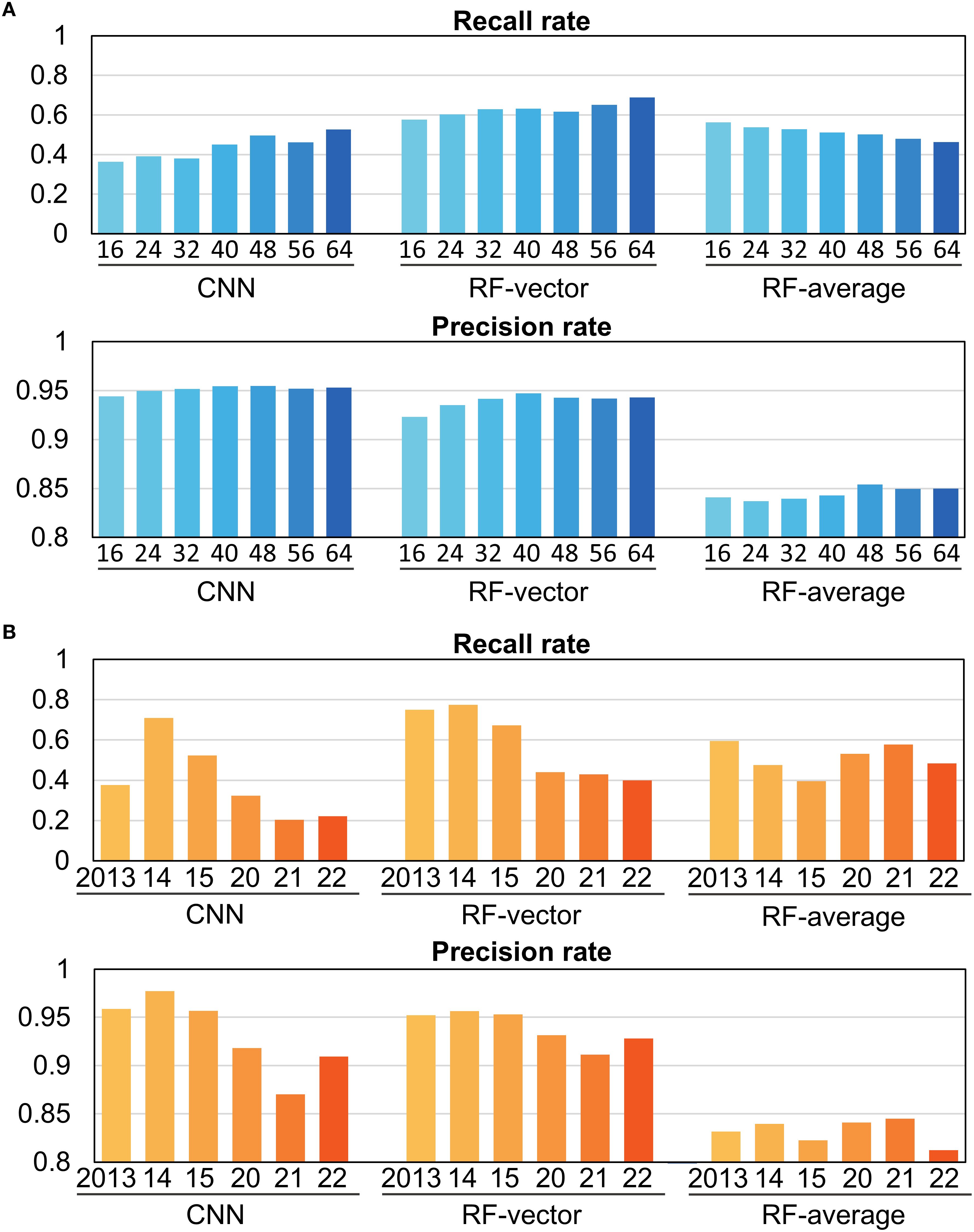
Figure 3. Validation of prediction accuracy by condition for each model. Bars represent the average of three Validations. (A) Accuracy of models by the number of grid cells (NC). The numbers below the bars indicate NC, the number of grid cells on one side of the square area (1 grid cell = 0.1 latitude and longitude degree). The type of model is specified below the numbers. (B) Validation of accuracy by year (2013 to 2022, excluding the training year) for models using range variables. Validation was performed using an NC of 40.

Jackknife analysis revealed that recall and precision were generally similar between the full models and those with individual variables excluded. However, excluding all water temperature variables led to a noticeable decline in performance across all models, highlighting its critical role in prediction (Figure 4, Supplementary Table S2). Excluding all water temperature variables led to deterioration in both recall and precision in CNN and RF-vector models, and caused a substantial drop in precision in the RF-averaged model. When water temperature was excluded by depth, only the RF-vector model showed a slight decrease in recall and precision for 30 m water temperature. No changes were observed when SSH and velocity were excluded.

Figure 4

Figure 4. Impact of variable removal on prediction accuracy. Conducted with three models displaying accuracy for all variables and accuracy when each variable is removed. Validation was performed using an NC of 40.

For all three models, predictions are expressed as the probability of fishing presence, ranging from 1.0 (high probability of saury catch) to 0.0 (low probability of saury catch). Figure 5 and Supplementary Figure S3 present prediction maps for September 18 and November 18, revealing seasonal and interannual trends. This seasonal movement trend, mirrored in the prediction map’s color intensity, is consistent across years (Supplementary Figure S4). Figure 6A shows a consistent monthly westward movement in the centroids of the actual and predicted fishing sites. It also illustrates an overall eastward shift when comparing the same month across different years. Comparing the first half of the fishing season (September 18) with the middle half (November 18), a similar eastward shift in the actual and predicted fishing sites is found (Figures 5, 6B, C). On September 18, the actual fishing sites consistently appeared west of 150°E until 2015 but shifted further offshore in 2020 (Figure 5). Based on the predictions by the CNN model, fishing sites with predicted probabilities exceeding 0.5 were located to the west of 150°E until 2015. Although the predicted probabilities in the east were lower compared to the western fishing sites, the predicted fishing sites have expanded to the east of 150°E since 2020. Similarly, in the RF-vector model, the predicted fishing sites expanded to the east post-2020. During the midterm fishing season on November 18, the actual fishing season gradually shifted to the east as the year progressed, and the prediction results showed a similar trend toward eastward movement. The predicted fishing sites identified by the RF-averaged are widely dispersed throughout the oceanic region, with minimal variation between years. The water temperature (0 m), SSH, and velocity on September 18 and November 18 are shown in Supplementary Figure S5 based on the data used for learning.

Figure 5

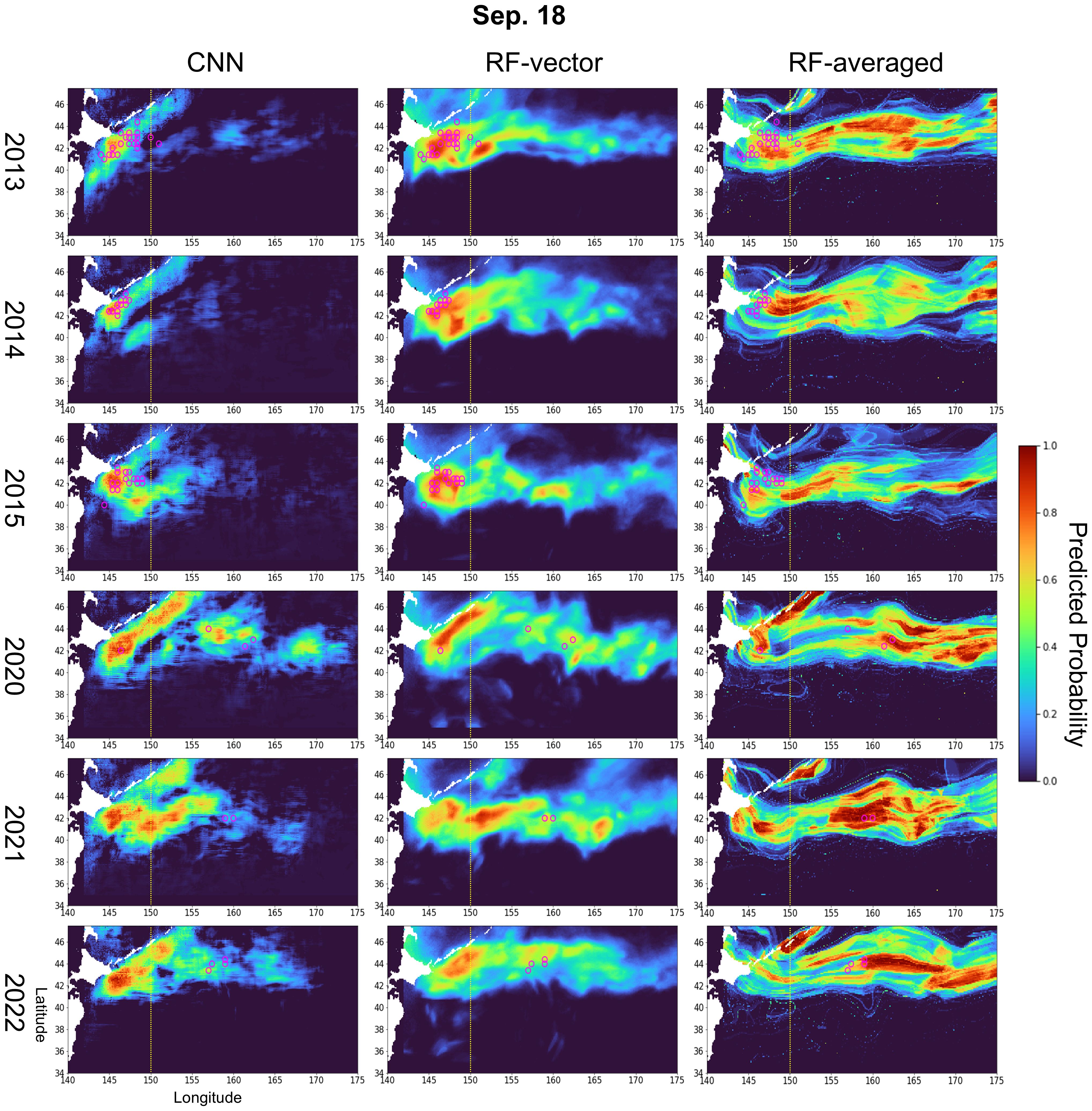
Figure 5. Prediction maps generated by models on September 18 for each year (2013–2015 and 2020–2022). Each grid cell’s color corresponds to the color bar and represents the predicted probability (range: 0–1). The overlaid magenta circles indicate locations where actual catches occurred. Prediction was performed using an NC of 40.

Figure 6

Figure 6. Monthly centroids of the actual and predicted fishing sites with regard to longitude. The actual fishing site centroids were determined using the fishing site location data, while the predictions were determined using the three models prediction probabilities. The centroids were calculated to validate the periods, excluding the learning period. The horizontal axis represents the month or year, while the vertical axis represents the longitude. Plots of consecutive months or years related to lines. (A) Monthly centroids of longitude during the validation period. (B) Centroids of longitude for September. (C) Centroids of longitude for November.

The feature importance in the random forest algorithm quantifies the extent to which each feature contributes to the reduction of impurities in the decision trees of the ensemble. Features that lead to a decrease in impurity when utilized in the trees are considered significant in the model. The RF-vector and RF-averaged importance index, obtained from impurity-based feature importances, is shown in Supplementary Figure S6 as a variable evaluation. Supplementary Figure S6, which presents the RF-vector and RF-averaged importance index, shows that the 10 m water temperatures represented by a distinct red color, were crucial for prediction. The RF-vector importance was divided by the variable type and displayed horizontally in the latitude direction and vertically in the longitude direction. The resolution and extent of the red area in the feature importance map were based directly on the spatial resolution of the environmental data (0.1° grid) used in the models. The red area extended from the center into an elliptical shape with a 5-grid cell radius (0.5° of longitude), corresponding to approximately 55.7 km (latitude) and 42.6 km (longitude) at 40°N.

4 Discussion

Models with multi-cell inputs, including RF-vector and CNN, more accurately tracked fishing site trends than spatial averaging models. RF-averaged, which used only spatially averaged values, showed lower accuracy compared to the RF-vector and CNN models using all the values from the square grid (Figure 3). Consequently, the RF-averaged model produced more scattered predictions across the study area (Figure 5 and Supplementary Figure S3). The superior performance of models that incorporate high-resolution grid data (RF-vector and CNN) suggests that gradient indicators, such as ocean currents, significantly impact predictions. Previous Pacific saury research emphasized the importance of large geographical scale changes (Tian et al., 2004; Miyamoto et al., 2019; Xing et al., 2022). The spatial scale of oceanographic factors (such as temperature, currents, and prey distribution) and the fish’s movement patterns and habitat selection are closely related. This suggests that setting variable ranges is particularly important for migratory Pacific saury (Pittman and Brown, 2011; Yasuda et al., 2014; Kakehi et al., 2020). As seen in Figure 3A, the RF-vector and CNN models showed increased precision when variables are set in a wide range, plateauing when number of grid cells is 40 or more. The spatial extent of important features shown in Supplementary Figure S6 aligns well with the daily swimming range of Pacific saury (64.8 km day⁻¹), enabling biological interpretation of spatial prediction patterns (Kakehi et al., 2020). The importance of water temperature within the Pacific saury’s daily activity range aligns with previous findings. Temperature and SSH showed high importance on the periphery and not only on the center. This suggests that including such peripheral areas, where key environmental features lie, may enhance predictive accuracy. These findings underscore the importance of using a sufficiently wide spatial range and maintaining the spatial resolution of environmental variables, instead of averaging them, when predicting catches.

Excluding the water temperature variable led to a decrease in recall and precision, which is a reasonable outcome given its known importance in Pacific saury distribution (Figure 4). Numerous reports suggest that Pacific saury’s habitat is affected by water temperature (Tian et al., 2004; Miyamoto et al., 2019; Yatsu et al., 2021). It is also been proposed that sea surface temperatures influence plankton density and juvenile fish growth (Ito et al., 2013; Miyamoto et al., 2020). However, when removing temperature at only one depth (e.g., 0, 10, or 30 m), the model performance remained largely unchanged. This suggests that water temperatures at different depths are highly correlated, and that the remaining layers can compensate for the excluded one. Thus, temperature as a whole remains a key variable in prediction, even though individual layers may be interchangeable. However, using all layers may still offer robustness under varying oceanographic conditions, such as changes in the vertical structure of the water column across years. Report suggest that the impact of SSH on Pacific saury distribution is less than that of temperature (Liu et al., 2022). However, despite numerous reports indicating ocean currents’ influence on distribution, it was unexpected that velocity had no significant effect on predictions (Oozeki et al., 2015; Liu et al., 2022). This implies that either temperature trends sufficiently explain the predictions or vertical and horizontal current velocities do not directly impact distribution.

It was particularly interesting to observe predictions reflecting the eastward shift of Pacific saury fishing points, a recent issue (Figures 5, 6). Environmental changes are believed to cause this eastward shift in Pacific saury fishing (Miyamoto et al., 2019; Hashimoto et al., 2020; Kakehi et al., 2020; Fuji et al., 2021). The observation of this eastward shift in predictions using marine factors suggests these factors contribute to the shift’s cause. To explore which conditions might have contributed to the model outputs, we compared the predicted fishing sites with the actual environmental fields (Supplementary Figure S5). On September 18 and November 18, the predicted sites were consistently located in areas with 0 m water temperatures ranging from 15°C–20°C. A large difference in SSH was observed around 2014–2015 and 2020–2022. In the later period, the predicted fishing sites were located in areas with low SSH (Supplementary Figure S5). The velocity also differed between the early and later period. The predicted fishing sites were located along the quasi-stationary jets (Isoguchi jets) in the latter period (Matsuta and Mitsudera, 2023). This pattern may indicate that environmental shifts in SSH and current structure, such as the position of the Isoguchi jets or the Oyashio flow, contributed to the eastward expansion of fishing grounds. Plants et al. described the second and third branches of the Oyashio flow into the Isoguchi stream, forming Lagrangian fronts where subtropical and subarctic waters converge, creating favorable fishing sites (Prants et al., 2020). The temperature distribution suitable for Pacific saury and the influence of the Kuroshio Current are consistent with known information (Ito et al., 2013; Liu et al., 2022). Therefore, the model may be capturing key environmental features associated with Pacific saury’s distributional shift. While the exact mechanisms remain speculative, such alignment suggests that this modeling approach could potentially aid in identifying drivers of spatiotemporal changes in fishery resources.

Near Japan’s coast at 143°E, both CNN and RF-vector predicted relatively high probabilities of fishing sites within the predicted spatial range across years (Figure 5 and Supplementary Figure S3). However, there have been nonfishing sites in this area post-2020, rendering these predictions incorrect. As shown in Figure 2, the training data were primarily concentrated along coastal regions, resulting in limited representation of offshore areas. This spatial imbalance likely caused the models to consistently predict high probabilities near the coast, possibly reflecting overfitting to coastal conditions. Additionally, while the significant difference was observed only in August and December, Mahalanobis distance was higher in low-catch years, suggesting notable oceanographic changes (Supplementary Figure S7). Environmental novelty may underlie the poorer performance in these years, particularly for RF-vector and CNN, which may have overfit to training conditions. The recall and precision rate deterioration in low-catch years, shown in Figure 3B, could be due to these effects. Previous studies have shown that environmental novelty can compromise SDM performance by limiting model generalizability (Allyn et al., 2025; Velazco et al., 2024). Furthermore, biased spatial sampling schemes such as those commonly present in fishery-dependent data may have reduced the representativeness of environmental conditions and increased uncertainty in projections (Karp et al., 2023).

These results demonstrate that prediction importance analysis can clarify not only the type of crucial environmental factors but also their range and depth. Among the models using spatial grids, the RF-vector model showed higher recall than the CNN, while the CNN had higher precision than the RF-vector model. The recall difference is larger than the precision difference, making RF-vector seem highly accurate. However, the CNN model reproduced the actual eastward shift more accurately. Therefore, the convolutional and pooling layers of the CNN model successfully extracted the characteristics of the ocean conditions.

5 Conclusion

The prediction model, utilizing two-dimensional spatial variables based on the ocean circulation model, demonstrated higher prediction accuracy compared to models without such spatial variables and visually replicated Pacific saury distribution behavior due to environmental factors. The significance and behavior of these models are anticipated to be beneficial for future Pacific saury resource assessment and management. In this study, a shift in Pacific saury fishing sites was identified based on data collected by the Japanese fishing fleet. However, it should be noted that fleets from other countries, such as Taiwan and China, have also increased their operations in the high seas in recent years. Therefore, to obtain a more comprehensive understanding of the spatial distribution and shifts in Pacific saury habitats, subsequent studies should incorporate fishing data from multiple nations. Such integrated data would enable more accurate modeling of how marine species respond to environmental variability across regions. The responsiveness of marine resources to environmental changes is crucial for environmental protection and resource management, and this study demonstrated that the machine learning prediction framework successfully captured spatial distribution shifts associated with these changes. In particular, accurate prediction models that capture offshore shifts and habitat changes are essential for developing climate-resilient fisheries management under future ocean warming scenarios. In the future, we aim to validate more precise models, assess how various fish species respond to environmental changes, and verify the practical application of a prediction tool for fishers using FRA-ROMS II prediction data.

Data availability statement

The FRA-ROMS data for researchers used as environmental variables can be used by submitting a usage request (https://fra-roms.fra.go.jp/fra-roms/). The exact location of the fishing grounds for Pacific saury data supporting the study findings are available from Japan Fisheries Agency but restrictions apply to the availability of these data, which were used under license for this study, and thus are not publicly available. However, data can be accessed from the authors upon reasonable request and with permission of Japan Fisheries Agency. The code used for learning and its usage was attached directly to the SI as a Supplementary Scripts.

Author contributions

TA: Writing – original draft, Writing – review & editing, Methodology. MM: Investigation, Writing – original draft, Writing – review & editing. TF: Investigation, Writing – original draft, Writing – review & editing. SS: Investigation, Supervision, Writing – original draft, Writing – review & editing.

Funding

The author(s) declare financial support was received for the research and/or publication of this article. This work was partially supported by the Fisheries Agency of Japan, but the study contents do not necessarily reflect the views of the Fisheries Agency.

Conflict of interest

The authors declare that the research was conducted in the absence of any commercial or financial relationships that could be construed as a potential conflict of interest.

Generative AI statement

The author(s) declare that no Generative AI was used in the creation of this manuscript.

Any alternative text (alt text) provided alongside figures in this article has been generated by Frontiers with the support of artificial intelligence and reasonable efforts have been made to ensure accuracy, including review by the authors wherever possible. If you identify any issues, please contact us.

Publisher’s note

All claims expressed in this article are solely those of the authors and do not necessarily represent those of their affiliated organizations, or those of the publisher, the editors and the reviewers. Any product that may be evaluated in this article, or claim that may be made by its manufacturer, is not guaranteed or endorsed by the publisher.

Supplementary material

The Supplementary Material for this article can be found online at: https://www.frontiersin.org/articles/10.3389/fmars.2025.1584413/full#supplementary-material

References

Allyn A. J., Brodie S. J., Mills K. E., Braun C. D., FarChadi N., McGarigal K., et al. (2025). Contrasting species distribution model predictability under novel temperature conditions. Divers. Distrib. 31, e70036. doi: 10.1111/ddi.70036

Crossref Full Text | Google Scholar

Baitaliuk A., Orlov A., and Ermakov Y. K. (2013). Characteristic features of ecology of the Pacific saury Cololabis saira (Scomberesocidae, Beloniformes) in open waters and in the northeast Pacific ocean. J. Ichthyol. 53, 899–913. doi: 10.1134/S0032945213110027

Crossref Full Text | Google Scholar

Behivoke F., Etienne M.-P., Guitton J., Randriatsara R. M., Ranaivoson E., and Léopold M. (2021). Estimating fishing effort in small-scale fisheries using GPS tracking data and random forests. Ecol. Indic. 123, 107321. doi: 10.1016/j.ecolind.2020.107321

Crossref Full Text | Google Scholar

Belgiu M. and Drăguţ L. (2016). Random forest in remote sensing: A review of applications and future directions. ISPRS J. Photogramm. Remote Sens. 114, 24–31. doi: 10.1016/j.isprsjprs.2016.01.011

Crossref Full Text | Google Scholar

Breiman L. (2001). Random forests. Mach. Learn. 45, 5–32. doi: 10.1023/A:1010933404324

Crossref Full Text | Google Scholar

Fuji T., Suyama S., Nakayama S., Hashimoto M., and Oshima K. (2021). A review of the biology for Pacific saury, Cololabis saira in the North Pacific Ocean. Available online at: https://www.npfc.int/system/files/2019-11/NPFC-2019-SSC%20PS05-WP13%28Rev%201%29%20Review%20of%20Pacific%20saury%20biology_Japan.pdf (Accessed June 2025).

Google Scholar

Fujii Y. and Kamachi M. (2003). Three).,dww.npfc. analysis of temperature and salinity in the equatorial Pacific using a variational method with vertical coupled temperature.npfc.int empirical orthogonal function modes. J. Geophys. Res. 108, 3297. doi: 10.1029/2002JC001745

Crossref Full Text | Google Scholar

Glaser S. M., Fogarty M. J., Liu H., Altman I., Hsieh C. H., Kaufman L., et al. (2014). Complex dynamics may limit prediction in marine fisheries. Fish Fisheries 15, 616–633. doi: 10.1111/faf.12037

Crossref Full Text | Google Scholar

Gobeyn S., Mouton A. M., Cord A. F., Kaim A., Volk M., and Goethals P. L. M. (2019). Evolutionary algorithms for species distribution modelling: A review in the context of machine learning. Ecol. Model. 392, 179–195. doi: 10.1016/j.ecolmodel.2018.11.013

Crossref Full Text | Google Scholar

Han H., Yang C., Jiang B., Shang C., Sun Y., Zhao X., et al. (2023). Construction of chub mackerel (Scomber japonicus) fishing ground prediction model in the northwestern Pacific Ocean based on deep learning and marine environmental variables. Mar. pollut. Bull. 193, 115158. doi: 10.1016/j.marpolbul.2023.115158

PubMed Abstract | Crossref Full Text | Google Scholar

Hashimoto M., Kidokoro H., Suyama S., Fuji T., Miyamoto H., Naya M., et al. (2020). Comparison of biomass estimates from multiple stratification approaches in a swept area method for Pacific saury Cololabis saira in the western North Pacific. Fish. Sci. 86, 445–456. doi: 10.1007/s12562-020-01407-3

Crossref Full Text | Google Scholar

Hirata H., Nishikawa H., Usui N., Miyama T., Sugimoto S., Kusaka A., et al. (2025). The Kuroshio large meander and its various impacts: a review. J. Oceanogr. 81, 165–185. doi: 10.1007/s10872-025-00753-z

Crossref Full Text | Google Scholar

Huang W.-B., Hsieh C.-H., Chiu T.-S., Hsu W.-T., and Chen C.-S. (2019). CPUE standardization for the Pacific saury (Cololabis saira) fishery in the Northwest Pacific. J. Mar. Sci. Technol. 27, 9. doi: 10.6119/JMST.201910_27(5).0009

Crossref Full Text | Google Scholar

Hubbs C. (1980). Revision of the sauries (Pisces, Scomberesocidae) with descriptions of two new genera and one new species. Fish. Bull. 77, 521–566.

Google Scholar

Ichii T., Nishikawa H., Mahapatra K., Okamura H., Igarashi H., Sakai M., et al. (2018). Oceanographic factors affecting interannual recruitment variability of Pacific saury (Cololabis saira) in the central and western North Pacific. Fish. Oceanogr. 27, 445–457. doi: 10.1111/fog.12265

Crossref Full Text | Google Scholar

Ito S., Okunishi T., Kishi M. J., and Wang M. (2013). Modelling ecological responses of Pacific saury (Cololabis saira) to future climate change and its uncertainty. ICES J. Mar. Sci. 70, 980–990. doi: 10.1093/icesjms/fst089

Crossref Full Text | Google Scholar

Ito S., Sugisaki H., Tsuda A., Yamamura O., and Okuda K. (2004). Contributions of the VENFISH program: meso-esoram:tions Pacific saury (Cololabis saira) and walleye pollock (Theragra chalcogramma) in the northwestern Pacific. Fish. Oceanogr. 13, 13ea. doi: 10.1111/j.1365-2419.2004.00309.x

Crossref Full Text | Google Scholar

Kakehi S., Abo J.-I., Miyamoto H., Fuji T., Watanabe K., Yamashita H., et al. (2020). Forecasting Pacific saury (Cololabis saira) fishing grounds off Japan using a migration model driven by an ocean circulation model. Ecol. Model. 431, 109150. doi: 10.1016/j.ecolmodel.2020.109150

Crossref Full Text | Google Scholar

Karp M. A., Brodie S., Smith J. A., Richerson K., Selden R. L., Liu O. R., et al. (2023). Projecting species distributions using fishery-dependent data. Fish Fish. 24, 71–92. doi: 10.1111/faf.12711

Crossref Full Text | Google Scholar

Kuroda H., Setou T., Kakehi S., Ito S.-I., Taneda T., Azumaya T., et al. (2017). Recent advances in Japanese fisheries science in the Kuroshio-Oyashio region through development of the FRA-ROMS ocean forecast system: Overview of the reproducibility of reanalysis products. Open J. Mar. Sci. 7, 62. doi: 10.4236/ojms.2017.71006

Crossref Full Text | Google Scholar

LeCun Y., Bengio Y., and Hinton G. (2015). Deep learning. Nature 521, 436–444. doi: 10.1038/nature14539

PubMed Abstract | Crossref Full Text | Google Scholar

LeCun Y., Boser B., Denker J. S., Henderson D., Howard R. E., Hubbard W., et al. (1989). Backpropagation applied to handwritten zip code recognition. Neural Comput. 1, 541–551. doi: 10.1162/neco.1989.1.4.541

PubMed Abstract | Crossref Full Text | Google Scholar

Liu Z. L., Jin Y., Yang L. L., Yuan X. W., Yan L. P., Zhang Y., et al. (2024). Improving prediction for potential spawning areas from a two-step perspective: A comparison of multi-model approaches for sparse egg distribution. J. Sea Res. 197, 102460. doi: 10.1016/j.seares.2023.102460

Crossref Full Text | Google Scholar

Liu S., Liu Y., Li J., Cao C., Tian H., Li W., et al. (2022). Effects of oceanographic environment on the distribution and migration of Pacific saury (Cololabis saira) during main fishing season. Sci. Rep. 12, 13585. doi: 10.1038/s41598-022-17786-9

PubMed Abstract | Crossref Full Text | Google Scholar

Matsuta T. and Mitsudera H. (2023). Kuroshio water intrusion into the subarctic region in the western North Pacific Ocean and analyses of the Lagrangian coherent structure. J. Oceanogr. 79, 629–636. doi: 10.1007/s10872-023-00696-3

Crossref Full Text | Google Scholar

Miyamoto H., Suyama S., Vijai D., Kidokoro H., Naya M., Fuji T., et al. (2019). Predicting the timing of Pacific saury (Cololabis saira) immigration to Japanese fishing grounds: A new approach based on natural tags in otolith annual rings. Fish. Res. 209, 167–177. doi: 10.1016/j.fishres.2018.09.016

Crossref Full Text | Google Scholar

Miyamoto H., Vijai D., Kidokoro H., Tadokoro K., Watanabe T., Fuji T., et al. (2020). Geographic variation in feeding of Pacific saury Cololabis saira in June and July in the North Pacific Ocean. Fish. Oceanogr. 29, 558–571. doi: 10.1111/fog.12495

Crossref Full Text | Google Scholar

NPFC Secretariat (2024). Summary footprint of Pacific saury fisheries. NPFC–2023–AR–annual summary footprint – pacific saury (Rev. 2022). Available online at: https://test.npfc.int/summary-footprint-pacific-saury-fisheries (Accessed June 2025).

Google Scholar

Oozeki Y., Okunishi T., Takasuka A., and Ambe D. (2015). Variability in transport processes of Pacific saury Cololabis saira larvae leading to their broad dispersal: Implications for their ecological role in the western North Pacific. Prog. Oceanogr. 138, 448–458. doi: 10.1016/j.pocean.2014.05.011

Crossref Full Text | Google Scholar

Pittman S. J. and Brown K. A. (2011). Multi-scale approach for predicting fish species distributions across coral reef seascapes. PloS One 6, e20583. doi: 10.1371/journal.pone.0020583

PubMed Abstract | Crossref Full Text | Google Scholar

Prants S., Kulik V., Budyansky M., and Uleysky M. Y. (2020). Relationship between saury fishing grounds and large-scale coherent structures in the ocean, according to satellite data. Izv. Atmos. Ocean. Phys. 56, 1638–1644. doi: 10.1134/S0001433820120506

Crossref Full Text | Google Scholar

Stock B. C., Ward E. J., Eguchi T., Jannot J. E., Thorson J. T., Feist B. E., et al. (2020). Comparing predictions of fisheries bycatch using multiple spatiotemporal species distribution model frameworks. Can. J. Fish. Aquat. Sci. 77, 146–163. doi: 10.1139/cjfas-2018-0281

Crossref Full Text | Google Scholar

Suyama S., Kurita Y., and Ueno Y. (2006). Age structure of Pacific saury Cololabis saira based on observations of the hyaline zones in the otolith and length frequency distributions. Fish. Sci. 72, 742–749. doi: 10.1111/j.1444-2906.2006.01213.x

Crossref Full Text | Google Scholar

Suyama S., Ozawa H., Shibata Y., Fuji T., Nakagami M., and Shimizu A. (2019). Geographical variation in spawning histories of age-1 Pacific saury Cololabis saira in the North Pacific Ocean during June and July. Fish. Sci. 85, 495–507. doi: 10.1007/s12562-019-01308-0

Crossref Full Text | Google Scholar

Tian Y., Akamine T., and Suda M. (2003). Variations in the abundance of Pacific saury (Cololabis saira) from the northwestern Pacific in relation to oceanic-climate changes. Fish. Res. 60, 439–454. doi: 10.1016/S0165-7836(02)00143-1

Crossref Full Text | Google Scholar

Tian Y., Ueno Y., Suda M., and Akamine T. (2004). Decadal variability in the abundance of Pacific saury and its response to climatic/oceanic regime shifts in the northwestern subtropical Pacific during the last half century. J. Mar. Syst. 52, 235–257. doi: 10.1016/j.jmarsys.2004.04.004

Crossref Full Text | Google Scholar

Tseng C.-T., Su N.-J., Sun C.-L., Punt A. E., Yeh S.-Z., Liu D.-C., et al. (2013). Spatial and temporal variability of the Pacific saury (Cololabis saira) distribution in the northwestern Pacific Ocean. ICES J. Mar. Sci. 70, 991–999. doi: 10.1093/icesjms/fss205

Crossref Full Text | Google Scholar

Tseng C.-T., Sun C.-L., Belkin I. M., Yeh S.-Z., Kuo C.-L., and Liu D.-C. (2014). Sea surface temperature fronts affect distribution of Pacific saury (Cololabis saira) in the Northwestern Pacific Ocean. Deep-Sea Res. II: Top. Stud. Oceanogr. 107, 15–21. doi: 10.1016/j.dsr2.2014.06.001

Crossref Full Text | Google Scholar

Velazco S. J. E., Rose M. B., De Marco P. Jr., Regan H. M., and Franklin J. (2024). How far can I extrapolate my species distribution model? Exploring shape, a novel method. Ecography 2024, e06992. doi: 10.1111/ecog.06992

Crossref Full Text | Google Scholar

Xing Q., Yu H., Liu Y., Li J., Tian Y., Bakun A., et al. (2022). Application of a fish habitat model considering mesoscale oceanographic features in evaluating climatic impact on distribution and abundance of Pacific saury (Cololabis saira). Prog. Oceanogr. 201, 102743. doi: 10.1016/j.pocean.2022.102743

Crossref Full Text | Google Scholar

Yasuda T., Yukami R., and Ohshimo S. (2014). Fishing ground hotspots reveal long-term variation in chub mackerel Scomber japonicus habitat in the East China Sea. Mar. Ecol. Prog. Ser. 501, 239–250. doi: 10.3354/meps10679

Crossref Full Text | Google Scholar

Yatsu A., Okamura H., Ichii T., and Watanabe K. (2021). Clarifying the effects of environmental factors and fishing on abundance variability of Pacific saury (Cololabis saira) in the western North Pacific Ocean during 1982–2018. Fish. Oceanogr. 30, 194–204. doi: 10.1111/fog.12513

Crossref Full Text | Google Scholar