Investigating SST diurnal variation and its response to the MJO in the North Indian Ocean using FY-4A data

Sea surface temperature (SST) diurnal variation is an important part of air-sea energy exchange, and its response to the Madden–Julian Oscillation (MJO) also helps in studying the development mechanism of the MJO. This study investigates SST diurnal variation in the North Indian Ocean by employing hourly data from the FY-4A geostationary satellite, in conjunction with reanalysis products and the MJO index. Validation against in situ SST measurements shows a bias of –0.33°C, an absolute bias of 0.73°C, an RSD of 0.33°C, an RMSE of 0.94°C, and a correlation coefficient of 0.90. The results demonstrate consistent accuracy throughout the diurnal cycle. Diurnal warming is most pronounced in the northern Arabian Sea and northern Bay of Bengal, especially from March to May prior to the monsoon onset. Wind speed and shortwave flux emerge as key drivers, although wind speed exerts a stronger regional influence on diurnal warming. Furthermore, the SST diurnal variation responds to the MJO within 1–2 days, as its active phase increases cloud cover and intensifies wind, thereby suppressing daytime warming. Despite the high temporal resolution of FY-4A, which allows for detailed sub-daily observations, monsoonal circulation and cloud cover can reduce data availability, complicating quantitative studies of SST variability and MJO feedbacks. Therefore, integrating multiple data sources is crucial for comprehensive analyses. Overall, these findings underscore the potential of geostationary satellites for monitoring diurnal SST fluctuations and emphasize the necessity of accounting for complex atmospheric–oceanic interactions in the North Indian Ocean when examining the role of diurnal variation in broader climate processes.

1 Introduction

The sea surface temperature (SST) diurnal variation, or diurnal warming, is generally defined as the daily temperature variation in the upper few meters of the ocean (Zhang et al., 2016b; Wick and Castro, 2020). SST diurnal variation, defined by sub-daily temperature fluctuations due to solar forcing and wind-driven mixing, is increasingly viewed as a critical regulator of air–sea interactions in tropical oceans. Early shipborne measurements revealed diurnal variation amplitudes exceeding 5°C under calm wind conditions (<3 m/s) in the western Pacific warm pool (Stramma et al., 1986), with such extremes altering latent heat fluxes by 20-30 W/m² through nonlinear thermodynamic relationships (Fairall et al., 1996). These discoveries raised fundamental questions about diurnal variation’s role in climate regulation, especially its capacity to influence atmospheric convection patterns (Bellenger and Duvel, 2012). While numerical models initially treated diurnal variation as a simple sinusoidal perturbation (Bernie et al., 2008), advances in coupled ocean-atmosphere modeling demonstrated that resolving the skin layer (0.01-1 mm) and subsurface warm layer (1-5 m) dynamics is essential for accurate diurnal variation representation (Clayson and Bogdanoff, 2013). The skin layer’s infrared-driven cooling effect (0.1–0.5°C), combined with heat accumulation in the warm layer from solar penetration, generates complex vertical temperature gradients that elude simplistic parameterizations (Moukomla, 2015).

Satellite-based measurements revolutionized research on diurnal variation through comprehensive global observations. Polar-orbiting sensors like MODIS and AVHRR enabled mapping of diurnal variation’s latitudinal dependence, revealing maximum amplitudes (3-5°C) in the tropical convergence zones and minimal variations (<0.3°C) in high-latitude regions (Gentemann et al., 2017). Microwave radiometers (AMSR-E/AMSR2) further quantified wind speed as the dominant control on diurnal variation variance (R²=0.65 globally), with residual variability attributable to solar zenith angle and mixed-layer depth (Minnett et al., 2019). However, these platforms faced critical temporal sampling constraints—with only 1–2 daily overpasses that aliased true DV signals, especially omitting afternoon SST peaks responsible for 60–70% of extreme daily heat flux (Donlon et al., 2012). This technological constraint persisted until geostationary satellites achieved sub-hourly monitoring, with Himawari-8’s 10-minute SST retrievals documenting typhoon-induced diurnal variation suppression in the western Pacific through continuous diurnal cycle tracking (Kurihara et al., 2016).

In the North Indian Ocean (NIO), diurnal variation dynamics are uniquely complex, influenced by monsoonal hydroclimate and the region’s distinctive basin geometry. During pre-monsoon months (March-May), surface wind speeds plummet to 2-3 m/s across the Arabian Sea while solar irradiance peaks at 850-950 W/m², creating ideal conditions for diurnal variation development (Sengupta and Ravichandran, 2001). RAMA buoy measurements during this period recorded diurnal variation amplitudes up to 4.2°C in the central Arabian Sea, with warming rates reaching 0.8°C/hour from 09:00 to 14:00 local time (Shenoi et al., 2009). The Bay of Bengal exhibits a contrasting regime with strong haline stratification (surface salinity<31 PSU) and shallow mixed layers (<10 m), which amplify near-surface temperature gradients by limiting vertical mixing (Thadathil et al., 2002, 2016). Here, diurnal variation develops within thin surface layers (<2 m), generating thermal inversions that persist for 6-8 hours daily (Girishkumar et al., 2014). Monsoon transitions dramatically alter these patterns - summer monsoon winds (June-September) suppress diurnal variation to<1°C through enhanced vertical mixing, while winter monsoon conditions permit moderate diurnal variation recovery (1.5-2°C) in sheltered coastal regions (Vialard et al., 2012). Crucially, the NIO’s semi-enclosed nature allows diurnal variation signals to persist longer than in open oceans, with observed phase lags of 2-3 hours in diurnal warming compared to adjacent equatorial regions (He et al., 2016; Wirasatriya et al., 2020).

The Madden–Julian Oscillation (MJO) introduces significant intraseasonal variability to the NIO diurnal variation system through coupled ocean–atmosphere feedbacks. During MJO suppressed phases over the Indian Ocean (Phases 2-3) (Wheeler and Hendon, 2004), reduced cloud cover increases surface shortwave radiation by 30-50 W/m² while concurrent wind speed reductions (<3 m/s) inhibit turbulent mixing (Demott et al., 2015). TOGA COARE/DYNAMO campaign observations captured Arabian Sea diurnal variation anomalies reaching +1.8°C under these conditions, with afternoon SST peaks occurring 2 hours earlier than climatological means (De Szoeke et al., 2015). Conversely, MJO active phases (Phases 5-6) generate wind bursts (>8 m/s) and deep convection, suppressing diurnal variation through mechanical mixing and cloud shading (Woolnough et al., 2000). Emerging high-resolution models indicate a bidirectional interaction—diurnal variation-induced surface flux perturbations can precondition MJO eastward propagation by modulating boundary layer moistening, causing climate models to underrate MJO speeds by 10–15% if diurnal variation processes are neglected (Dasgupta et al., 2021; Demott et al., 2015; Li et al., 2020). This scale-interactive relationship presents a critical challenge for subseasonal forecasting, as traditional daily SST products smooth out diurnal variation signals that may enhance or dampen MJO development.

Recent technological advancements in geostationary satellites offer unprecedented capabilities to resolve diurnal variation-MJO interactions. The GOES-R series demonstrated 0.3°C accuracy in tracking afternoon SST peaks across the eastern Pacific through 5-minute temporal resolution (Luo and Minnett, 2021; Yu et al., 2021), while Himawari-8 revealed typhoon-induced diurnal variation suppression mechanisms through continuous 10-minute observations (Kurihara et al., 2016). China’s FY-4A satellite, operational since 2018, represents a paradigm shift for NIO studies. Its Advanced Geostationary Radiation Imager (AGRI) delivers 4 km SST retrievals every 10 minutes in the Indian Ocean sector (70°E–140°E) and offers three major advantages over legacy systems: (1) enhanced atmospheric correction using 12 spectral bands (including 3 thermal infrared channels), reducing cloud contamination errors by 40% relative to MODIS (Xu et al., 2020); (2) Stable viewing geometry eliminating orbital stitching artifacts that removes polar-orbiter composites; (3) Synergistic use with microwave sensors (AMSR2) enabling all-weather retrievals, overcoming persistent cloud cover during monsoon seasons (Li et al., 2022). Although FY-4A has been validated for land surface monitoring (Liu et al., 2023), its oceanographic applications remain underexplored, particularly regarding diurnal variation characterization and climate interaction studies.

Despite these advancements, critical knowledge gaps persist in understanding NIO’s diurnal variation system. Existing regional climatologies rely heavily on polar-orbiting satellite data with inherent temporal aliasing, potentially underestimating true diurnal variation magnitudes by 15-20% (Gentemann et al., 2017). MJO-diurnal variation coupling mechanisms remain poorly constrained observationally, as most studies rely on reanalysis products that underrepresent diurnal cycles (Wirasatriya et al., 2020). Furthermore, the relative contributions of wind speed versus solar radiation to diurnal variation variability remain contested - while buoy studies emphasize wind control (R²=0.65 in Arabian Sea; Ajith Joseph et al., 2019), model simulations suggest radiation dominates (60-70%) in stratified regions like the Bay of Bengal (Thadathil et al., 2016). This uncertainty highlights the urgent need for high-resolution observational data spanning various monsoonal regimes.

This study examines the characteristics of SST diurnal variation in the North Indian Ocean and its response to the MJO using FY-4A geostationary satellite observations, underscoring the benefits of high-resolution geostationary platforms for SST diurnal variation research. The remainder of this article is organized as follows: Section 2 details the data and methodology, Section 3 presents the FY-4A SST validation results, Section 4 outlines the North Indian Ocean diurnal variation patterns, Section 5 explores influencing factors and MJO coupling, and Section 6 concludes.

2 Data and methods

2.1 Data

2.1.1 FY-4A SST data

Chinese FY-4A satellite, a new-generation geostationary meteorological platform, was launched on December 11, 2016, from Xichang and successfully located at 99.5°E, 35,786km above the equator on December 17, 2016. For early operational readiness, FY-4A commenced drifting at 104.7°E above the equator on May 25, 2017. It is equipped with the Advanced Geostationary Radiation Imager (AGRI), the Geostationary Interferometric Infrared Sounder (GIIRS), the Lightning Mapping Imager (LMI), and the Space Environment Monitoring Instrument Package (SEP). Equipped with 14 bands, the AGRI captures visible and infrared images from 62.36°S to 62.36°N between 43.42°E to 165.98°W (fulldisk observation range, Figure 1), spanning almost the entire Indian Ocean and parts of the eastern Pacific Ocean. The AGRI’s observation frequency of the full disk is 1 hour and the AGRI takes 3 consecutive full-disk observations every 3 hours. The AGRI also conducts regional observation of China every 5 minutes when there is no full-disk observation. Therefore FY-4A satellite can acquire 40 full-disk images and 165 regional images of China (3°N-55°N, 60°E-137°E) every day.

Figure 1

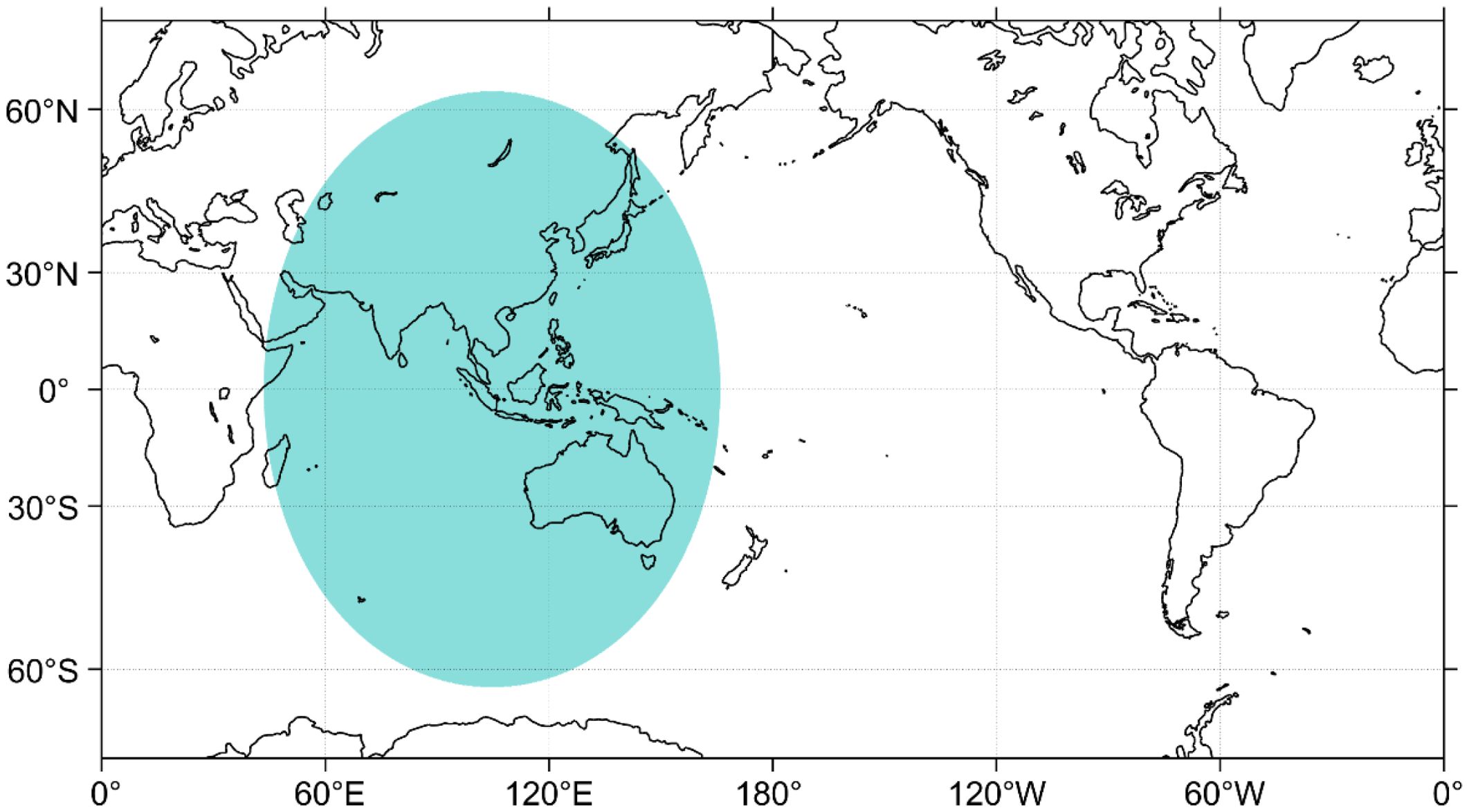
Figure 1. FY-4A full disk observation area (blue).

Currently, AGRI Level-1 data and 25 Level-2 products, including cloud coverage, land surface temperature, and sea surface temperature, are publicly available. Users can access them freely from http://data.nsmc.org.cn/. The operational FY-4A SST products used in this study were available to the public on January 18, 2019. FY-4A SST retrievals utilize three infrared (3.7, 10.8, and 12.0 μm) bands. Each FY-4A SST file includes a quality flag: 0 (good pixel), 1 (sub-optimal), 2 (bad), or 3 (invalid), indicating the data reliability at each pixel. In this study, we select 8678 available full-disk SST data with a spatial resolution of 4 km and a temporal resolution of 1 hour, covering the entire year of 2020, and only SST pixels flagged with quality 0 are used. The study region is the North Indian Ocean (NIO: 0°N–30°N, 35°E–105°E), with observations spanning January 1 to December 31, 2020.

2.1.2 In situ data

To validate FY-4A SSTs, in situ SSTs from the In situ SST Quality Monitor (iQuam) project are used as reference data in this study. The iQuam dataset, developed by NOAA, supports the calibration and validation (Cal/Val) of satellite-retrieved SSTs. The iQuam project collects in situ SST data from different platforms including Argo, Drifter, IMOS ships, etc, and the same quality control (QC) algorithm was designed to process different in situ SSTs for minimizing in situ measurement error (Xu and Ignatov, 2014; Tu and Hao, 2020). The quality flags (1-5: invalid, not used, not used, low quality, acceptable) are used to specify QCed SSTs.

In this study, we use drifting buoy SSTs for satellite validation due to their large numbers and measurement depths of only a few tens of centimeters—closer to the sea surface than moored buoys or ships (Zhang et al., 2016b). To minimize errors, only the best quality (quality flag level=5) drifting buoy SSTs are obtained to use from https://www.star.nesdis.noaa.gov/socd/sst/iquam/data.html.

2.1.3 Meteorological data

The wind speed at 10 m height above sea level and solar shortwave flux (SWF) data used in this study are from the ERA5 dataset. ERA5 is the fifth-generation ECMWF reanalysis for the global climate and weather, which provides hourly estimates for a large number of atmospheric, oceanic, and land-surface parameters (Hersbach et al., 2020). All ERA5 datasets are publicly available at https://cds.climate.copernicus.eu/. In this study, we collect hourly wind speed and solar shortwave flux (SWF) of the year 2020 to discuss the factors affecting the diurnal variation of sea surface temperature. They feature a spatial resolution of 0.25° × 0.25°. The time in ERA5 data is in coordinated universal time (UTC). We convert UTC to local solar time (LST) using LST = UTC + (longitude × 4 min), consistent with the approach used elsewhere in this study.

2.2 Methods

2.2.1 QC and matchup

Several quality control (QC) steps are applied to both FY-4A SST and in situ data prior to use in this study. First, only the highest quality data of both FY-4A SST data and in situ data are selected, and the highest quality level of FY-4A SST data and iQuam SST data selected are 0 and 5 respectively. Next, for FY-4A SST data, we retain only those pixels that have at least one neighboring pixel with quality=0, mitigating the influence of cloud edges and sensor errors. Finally, SST derived from the AGRI is called “skin SST” since the AGRI measures temperatures in the top 10-20 μm of the ocean. In situ SST from drifting buoys reflects the temperature at 20–30 cm depth, commonly referred to as “bulk SST” (Kawai and Wada, 2007; Zhang et al., 2016b). “Bulk SST” tends to be less than “skin SST” due to the cool-skin effect (Fairall et al., 1996; Kawai and Wada, 2007). In this study, we add a 0.17°C offset to all FY-4A SSTs to correct the cool-skin effect, as also employed by Beggs and Zhang (Beggs et al., 2012; Zhang et al., 2016b).

After the QC steps, the FY-4A SSTs are ready to be validated with the iQuam SSTs. First, all in situ SSTs located within the full disk range are extracted to reduce the amount of matchup data. We then apply a 2 km × 2 km spatial window and a 30-minute temporal window for matching satellite and in situ SSTs. Then the satellite SST pixel point with the closest distance to each in situ SST data is selected to generate the matchup pair.

2.2.2 Diurnal variation of SST

The diurnal variation of sea surface temperature is the difference between the SST at a given moment of the day and the reference SST also called the foundation SST (SST_fnd). The foundation SST (SST_fnd) is defined as the temperature of the water column without diurnal temperature variability (diurnal warming or diurnal cooling) (Rayner et al., 2007; Kawai and Wada, 2007). Determining SST_fnd precisely remains challenging, and there are two main estimation approaches (Zhang et al., 2016a). One approach uses the closest pre-dawn SST value as SST_fnd (Karagali and Høyer, 2014; Zhang et al., 2016a, 2016), while the other (“multiday”) considers spatial–temporal coverage to define SST_fnd (Castro et al., 2014; Wick and Castro, 2020). In this article, the pre-dawn SSTs of FY-4A are collected for SST_fnd calculation and a night-time window is applied to calculate the mean pre-dawn SST in order to increase the amount of effective data. The night-time window is set from 00:30 LST to 05:30 LST on the same local day from Zhang et al (Zhang et al., 2016a). And we calculate diurnal variation of SST as

$$\text{dSST}={\text{SST}}_{\text{t}}-{\text{SST}}_{\text{f}\text{n}\text{d}}$$

where dSST is the diurnal variation of sea surface temperature, and SST_t is the FY-4A SST at a given moment of the day. Moreover, dSST_max is the maximum dSST of the day.

2.2.3 Identify MJO activity

The Madden–Julian Oscillation (MJO) consists of two primary phases: an active phase with substantial precipitation, and a suppressed phase with reduced precipitation. Based on global tropical data, Wheeler and Hendon have categorized the MJO into eight distinct phases, with two of these phases occurring within the Indian Ocean (Wheeler and Hendon, 2004). In this study, the real-time multivariate MJO (RMM) index from the Australian Bureau of Meteorology was utilized to obtain the active phases and active intensity of the MJO in the tropical Indian Ocean. This index is the most commonly used for MJO monitoring and forecasting. The index is derived from the projection of the day-by-day data onto the first two multivariate EOF modes of 850-hPa latitudinal wind (u850), 200-hPa latitudinal wind (u200), and OLR after latitudinal averaging in the tropics (15°S~15°N). The standardized time series is then used to calculate the RMM indices, denoted as RMM1 and RMM2, respectively. Notably, all these data exclude annual cycles and interannual variations. The latitudinal propagation of the strong MJO along the global tropics can be divided into eight spatial phases based on the two-dimensional phase space defined by RMM1 and RMM2. The geographical location of the MJO can be represented by a point in the two-dimensional phase space defined by the RMM1 and RMM2 indices. The distance of a point from the phase space center reflects MJO amplitude, indicating its strength. The eight phases are analogous to specific stages in the life cycle of the MJO, signifying the eastward propagation of MJO convection from the Indian Ocean to the Pacific Ocean.

3 Validation

Validation is essential before using FY-4A SST data in subsequent analyses. Mean bias, absolute bias, robust standard deviation (RSD), root mean square error (RMSE), and correlation coefficient (R) are the statistical parameters used to quantify the differences between FY-4A and in situ SST. These metrics are widely applied in satellite SST validations (Ye et al., 2021; Zhang et al., 2016a; Tu and Hao, 2020; Swapna et al., 2022; Ditri et al., 2018). A Gaussian probability density function is fitted to the bias data to obtain the RSD, which helps characterize most of the dataset (Merchant et al., 2008; Ye et al., 2021). The validations for the FY-4A SST in the full disk and the North Indian Ocean are as follows, respectively.

3.1 Full-disk

The FY-4A’s full-disk image can cover almost the whole Indian Ocean and the western Pacific Ocean. The full-disk SSTs derived from FY-4A are validated with in situ SSTs observed from drifters. The “cool skin” effect is also considered by a constant 0.17°C. Figure 2a shows the spatial distribution of all matching points and almost all matching points between FY-4A SST and in situ SST have a negative bias, except for those on the Southern Indian Ocean, and the bias values are within -2°C - 2°C. Because the diurnal variation in sea surface temperature depends heavily on hourly SST (SST_t), we computed the percentage of FY-4A full-disk SST observations collected at each hour (Figure 2b). The results show that they are evenly distributed in each period, with a frequency of about 4% and no obvious data missing. The SST data during 17:00-21:00 LST are relatively more, with a frequency close to 5%. However, the data during this period were not used to calculate SST_fnd, and thus they do not affect subsequent results. The distribution of bias between the FY-4A full-disk SST and the in situ SST is depicted in Figures 2c, d. The bar plot displays a normal distribution of bias between -4°C - 4°C, and the scatter density plot shows a good agreement between the FY-4A SST and the in situ SST. Additionally, Table 1 presents monthly and annual statistical results for 2020. Over the entire year of 2020, 306,569 matching points yielded a mean bias of -0.30°C, absolute bias of 0.77°C, RMSE of 0.99°C, RSD of 0.35°C, and R of 0.99. The statistical results also show that the FY-4A SST data are in good consistency with the in situ data. In particular, the high correlation between FY-4A full-disk SST and in-situ SST indicates the high quality of FY-4A SST data, which will also provide higher reliability for subsequent analysis. However, even after the cool-skin effect was adjusted for using constant values, the statistical results for all months reveal that the negative deviation is still caused by the a strong cool-skin impact in specific temperature ranges.

Figure 2

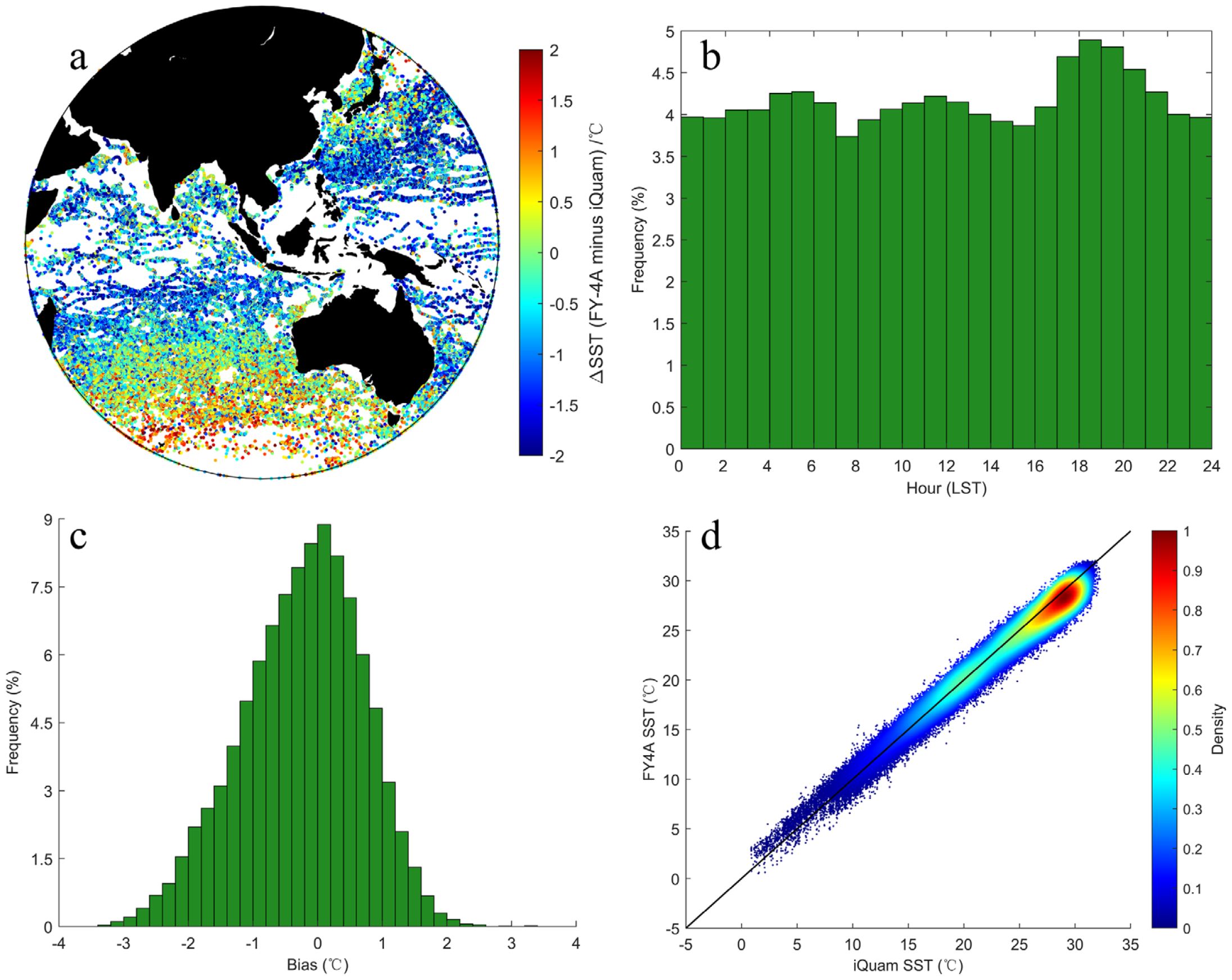
Figure 2. Results of FY-4A full-disk SST vs iQuam validation: (a) spatial distribution of all matched validation points of FY-4A vs. iQuam; (b) frequency distribution of matched points per hour at local solar time (LST); (c) bias distribution of matched points; (d) scatter density plot of FY-4A vs. iQuam SST;.

Table 1

Table 1. Statistics of both in-situ validation.

To emphasize the deviations, Figure 3a plots the difference between FY-4A SST and iQuam SST on the y-axis and the range of iQuam SST on the x-axis. The scatter density plot shows that the deviations are all distributed around the y=0 line, but the negative deviations are more discrete in the range of 26°C - 32°C of iQuam SST. In Figure 3b, the mean bias transitions from positive to negative with increasing iQuam SST. The 25th and 75th quartile intervals of deviation become wider, especially when the iQuam SST is in the range of 26°C - 31°C, the number of collection points reaches the maximum and the negative deviation increases further. In the extreme high-SST interval (iQuam SST > 30), the number of collection points starts to drop sharply due to limited extreme high-temperature events, but the negative deviation still increases further, presumably because of the significant cold skin effect that may contribute more to the negative deviation.

Figure 3

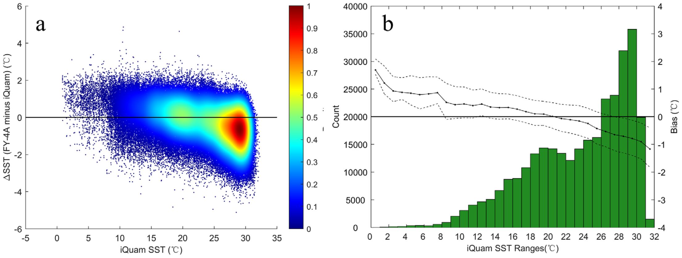
Figure 3. Results of FY-4A full-disk SST vs iQuam cross-validation: (a) scatter density plot. The y axis is the FY-4A data minus iQuam data and the x axis is the iQuam data; (b) collocation numbers, bias (solid line) and STDs (dotted line) over different iQuam SST ranges.

3.2 The North Indian Ocean region

Given that the main study area of SST diurnal variation in this paper is in the North Indian Ocean, we specifically collected and validated data of FY-4A SST in this region (Figure 4a). Due to the special climatic characteristics and sea-air conditions in this region, the amount of effective data becomes very limited from summer, but 36109 data points from the year 2020 are still collected for matching validation. Figure 4b shows that the frequency range of the matched data points at different periods is 3.5% - 5%, and the distribution of data points during 11:00 - 14:00 and 21:00 - 01:00 is relatively small compared with other periods, less than 4%. The histograms and scatter density plots of the deviations between FY-4A SST and iQuam SST for the North Indian Ocean region are in Figures 4c, d, respectively. The statistical results show that the SST is higher in the North Indian Ocean throughout the year with a mean value, ranging from 22°C - 33°C. The consistency between FY-4A SST and in-situ SST in this region is slightly worse than that of the full disk, with a bias of -0.33°C, absolute bias of 0.73°C, RSD of 0.33°C, RMSE of 0.94°C, and R of 0.90. This discrepancy may be attributed to unique climatic conditions and air–sea interactions, which reduce the number of matching data points and widen the gap between near-surface water temperature and skin temperature.

Figure 4

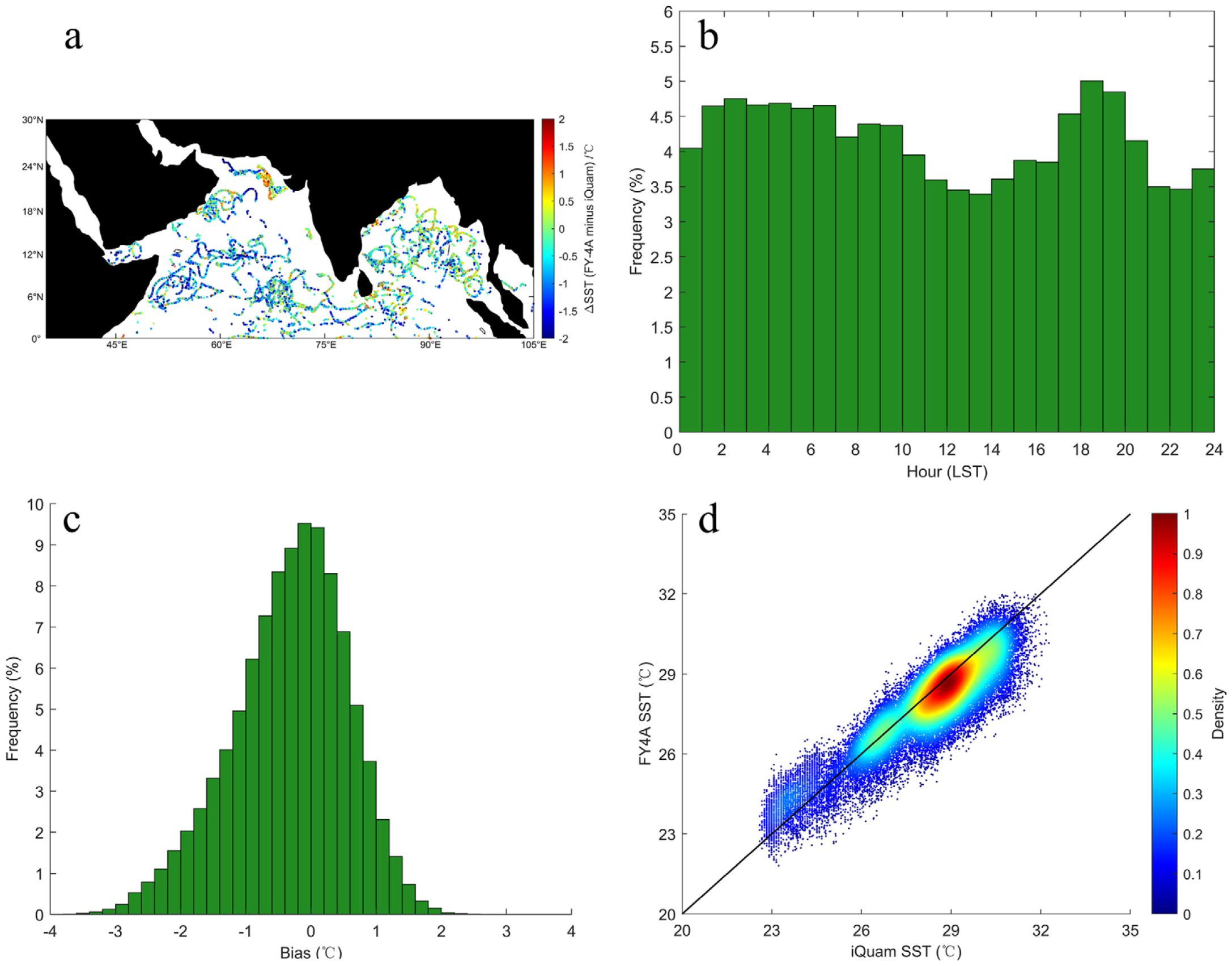
Figure 4. Results of FY-4A vs iQuam validation in the NIO: (a) spatial distribution of all matched validation points of FY-4A vs. iQuam; (b) frequency distribution of matched points per hour at local solar time (LST); (c) bias distribution of matched points; (d) scatter density plot of FY-4A vs. iQuam SST;.

Figure 5 illustrates how deviations vary across different iQuam SST intervals. The dispersion of the deviation distribution is larger than that of the full disk, and the deviation is still mainly negative in the high-SST region. The trend of the deviation of FY-4A SST from the in-situ SST in the North Indian Ocean region is similar to that of the full disk in that the deviation changes from positive to negative and the absolute value increases gradually with the increase of temperature, and the 25^th and 75^th quartile intervals of the deviation become wider.

Figure 5

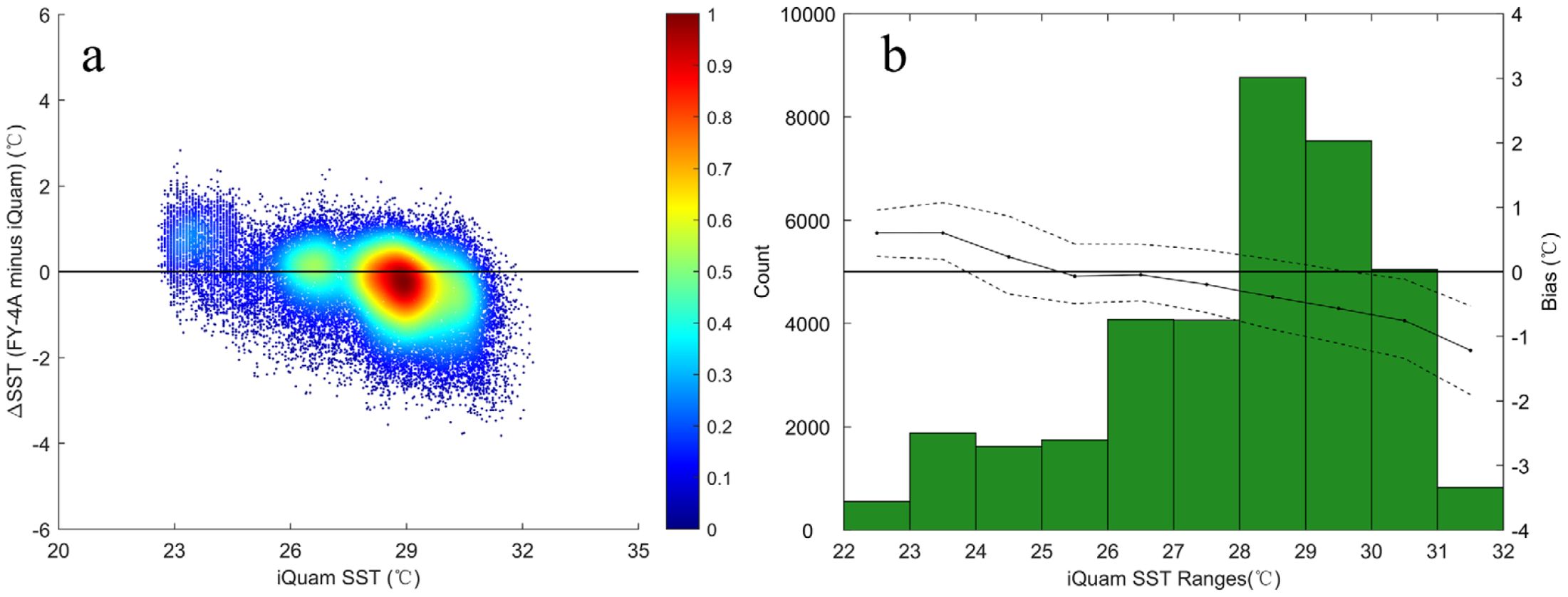
Figure 5. Results of FY-4A vs iQuam cross-validation in the NIO: (a) scatter density plot. The y axis is the FY-4A data minus iQuam data and the x axis is the iQuam data; (b) collocation numbers, bias (solid line) and the 25^th and 75^th quartile intervals of the deviation (dotted line) over different iQuam SST ranges.

Overall, the full-disk validation confirms that FY-4A SST data exhibit strong stability. In the North Indian Ocean region, validation indicates acceptable errors, supporting the use of FY-4A SST data in subsequent diurnal variation analyses.

4 Results

4.1 Spatial patterns of dSST in the NIO

Given the discrete distribution of diurnal warming events, we used the validated FY-4A SST dataset to calculate daily dSST in the North Indian Ocean for 2020. After removing invalid data, we computed the monthly mean dSST values and generated the corresponding spatial distributions, as illustrated in Figure 6. For clarity, diurnal warming events were classified into four categories: weak diurnal warming (0°C< dSST< 1°C); general diurnal warming (1°C< dSST< 2°C); strong diurnal warming (2°C< dSST< 3°C); extreme diurnal warming (dSST > 3°C).

Figure 6

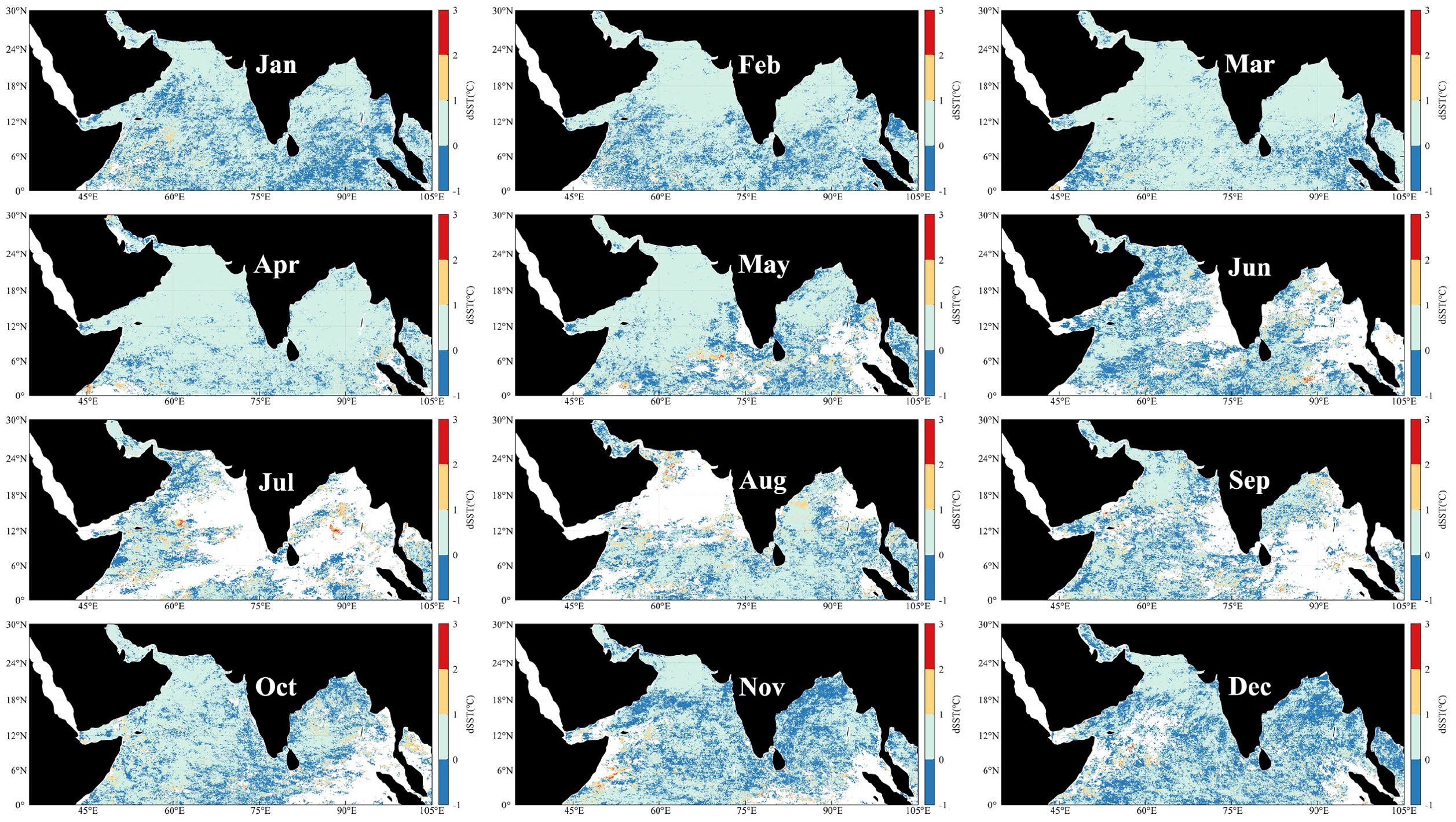
Figure 6. Distribution of monthly mean dsst in the North Indian Ocean in 2020 (January-December).

Figure 6 illustrates the principal regions and extent of diurnal warming in the North Indian Ocean during 2020. It demonstrates that the Bay of Bengal Sea and the Arabian Sea are particularly susceptible to significant diurnal warming. In general, diurnal warming events exhibit a broad and relatively continuous spatial distribution. The spatial distribution of strong diurnal warming events is characterized by discrete and small areas. The northern part of the Arabian Sea and the area in the vicinity of the Gulf of Oman exhibit weak diurnal warming throughout the year. In contrast, stronger diurnal warming events appear mostly in the mid- to low-latitude areas of the North Indian Ocean.

Figure 6 highlights the main regions and extent of diurnal warming in the North Indian Ocean during 2020, demonstrating that the Bay of Bengal and the Arabian Sea are especially susceptible to significant diurnal warming. In general, diurnal warming events exhibit a broad and relatively continuous spatial distribution, whereas stronger diurnal warming events appear mostly in the mid- to low-latitude areas. The northern Arabian Sea seems more prone to diurnal warming events. Nevertheless, most events in this region fall within a weak warming range (dSST 0–1°C). Extreme diurnal warming events (dSST > 3°C) are observed off the Somali Peninsula, in the Bay of Oman, the central Bay of Bengal, and near the equator. Compared with general diurnal warming, these stronger events are more episodic and localized.

4.2 Seasonal patterns of dSST in the NIO

As shown in Figure 6, monthly mean dSST coverage can reach nearly 100% from January through April, but drops to below 60% from July to September, with July being the lowest at about 40%. To further examine diurnal warming frequency, we counted the number of days (dSST > 0) per month in 2020 for the North Indian Ocean (Figure 7). The results indicate heightened susceptibility from January to May. Specifically, February, March, and April see most of the Arabian Sea and Bay of Bengal experiencing more than 15 days of diurnal warming per month. This prevalence diminishes sharply in May, and from June to September, the North Indian Ocean exhibits the lowest frequency of diurnal warming all year, averaging fewer than five days per month. Beginning in October, the frequency of diurnal warming gradually rises, with more than 15 warming days per month recorded mostly in the northern Arabian Sea and the Bay of Bengal. Overall, the North Indian Ocean is more susceptible to diurnal warming from January through May, whereas summer shows the lowest probability of widespread diurnal warming.

Figure 7

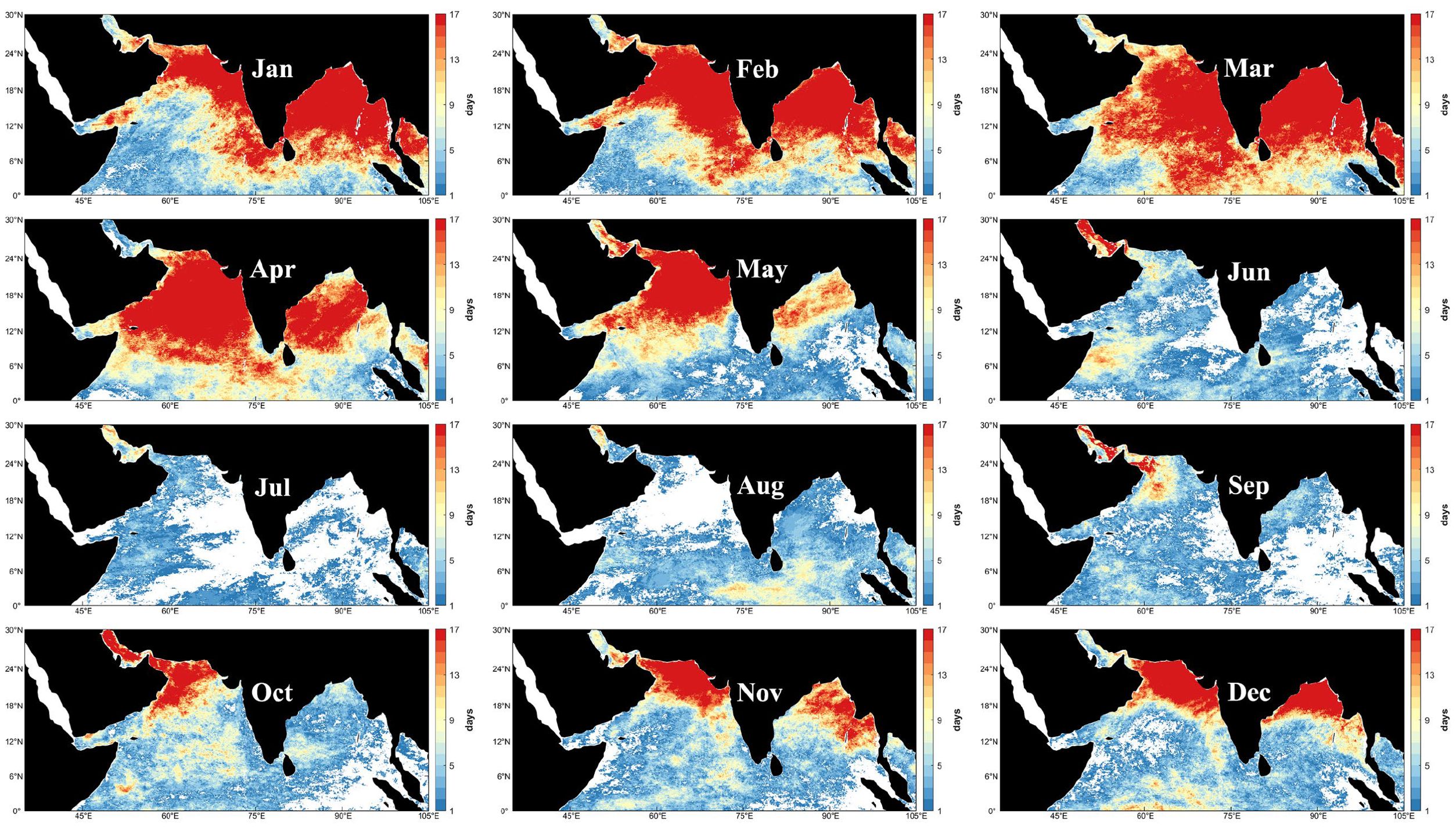
Figure 7. Distribution of the number of days per month in which diurnal warming occurs in the North Indian Ocean in 2020.

To evaluate diurnal warming at a finer level, Figure 8a depicts monthly changes in pixel counts across different dSST ranges, while Figure 8b presents the corresponding dSST percentages among pixels exhibiting diurnal warming. Overall, diurnal warming in the North Indian Ocean displays notable seasonal variations, with spring (February–April) featuring the widest regional extent, regardless of warming intensity. However, when examining the proportion of pixels by warming intensity, July—which records the fewest total warming pixels—shows a much higher share of strong (2–3°C) or extreme (>3°C) diurnal warming relative to other months. In contrast, the proportion of general diurnal warming (1–2°C) remains relatively stable throughout the year.

Figure 8

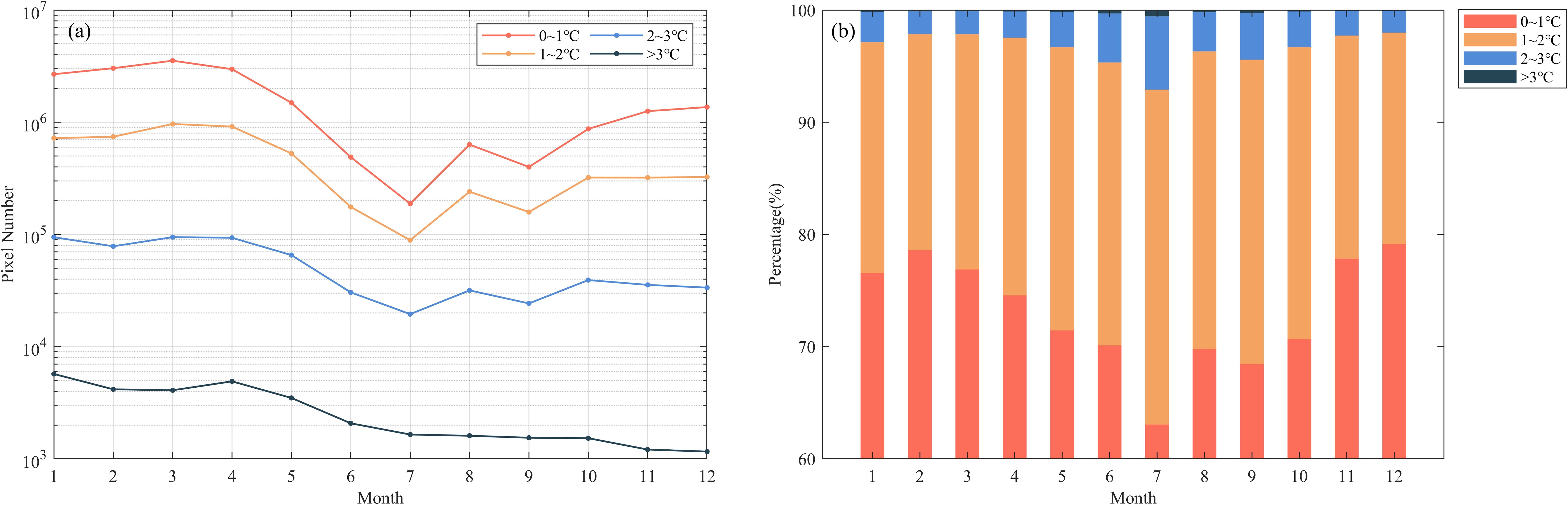
Figure 8. Inter-monthly variability of different degrees of diurnal warming in the North Indian Ocean in 2020: (a) change in the number of points collected each month for different degrees of diurnal warming; (b) change in the proportion of different degrees of diurnal warming(weak diurnal warming: 0-1°C; general diurnal warming: 1-2°C; strong diurnal warming: 2-3°C; extreme diurnal warming: > 3°C).

5 Discussion

5.1 Impact factors of diurnal variation events

Numerous studies have shown that wind speed and solar shortwave radiation directly impact the diurnal warming of sea surface temperature (SST): higher wind speeds dampen diurnal warming via enhanced mixing, whereas greater shortwave radiation intensifies warming (Seo et al., 2014; Zhang et al., 2016b, 2016; Hsu et al., 2021; Shenoi et al., 2009). To examine the spatial and seasonal characteristics of diurnal warming in the North Indian Ocean, we analyzed wind speed and solar shortwave radiation flux data from ERA5.

5.1.1 Wind speed

The North Indian Ocean features a monsoon climate, characterized by northeasterly winds in winter and southwesterly winds in summer; consequently, any analysis of diurnal warming must consider the region’s unique climatic conditions. Figure 9 illustrates the monthly average wind distribution in 2020, revealing clear seasonal patterns. March and April experience markedly low wind speeds (<6 m/s) across the Arabian Sea, the Bay of Bengal, and the tropical Indian Ocean, with many areas falling below 4 m/s—favorable conditions for diurnal SST warming. By contrast, June through August see significantly higher wind speeds, often exceeding 10 m/s in the Arabian Sea and exceeding 6 m/s in the Bay of Bengal. Simulation results from Zhang et al. indicate that diurnal warming rarely occurs at wind speeds above 6 m/s, suggesting that high winds constitute a primary inhibiting factor in the North Indian Ocean during this period. The seasonal characteristics of SST warming in the North Indian Ocean (Figures 6, 8) corroborate these conclusions.

Figure 9

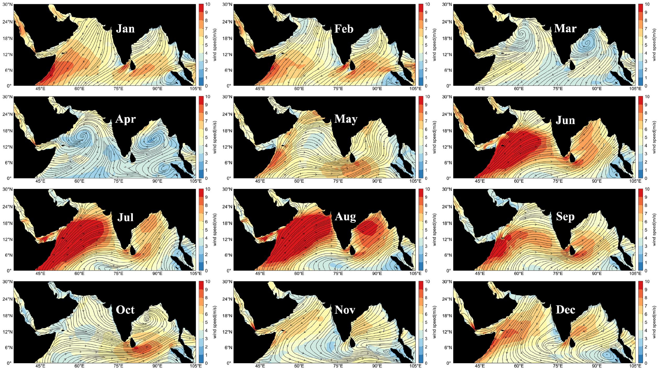
Figure 9. Distribution of monthly mean daytime wind speed in the North Indian Ocean in 2020, obtained by averaging the wind speed from 07:00 to 17: 00 local time each day.

5.1.2 Shortwave flux

Shortwave radiation serves as the principal energy source driving SST diurnal variation, with intraday fluctuations acting as a key trigger. Figure 10 shows the monthly mean distribution of shortwave radiative fluxes in 2020, which exhibits marked seasonal variation. From March to May, shortwave fluxes surpass 400 W/m² across most of the North Indian Ocean, whereas from June onward, much of the Arabian Sea and Bay of Bengal experience fluxes below 300 W/m². By July, flux values across the region do not exceed 350 W/m², hindering diurnal SST warming. Beginning in August and extending through December, higher shortwave fluxes concentrate primarily in low-latitude waters.

Figure 10

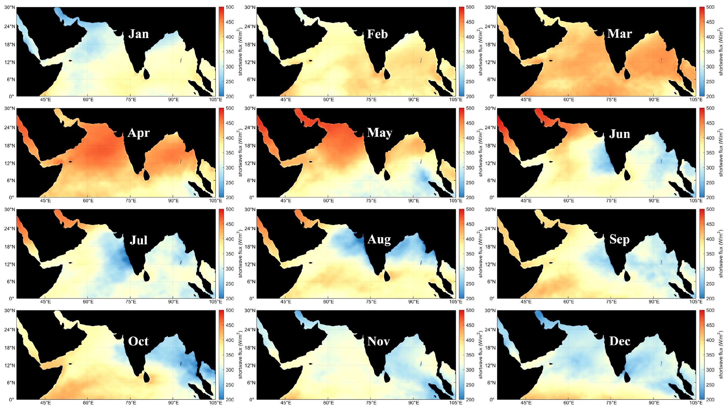
Figure 10. Distribution of monthly mean shortwave radiation fluxes at sea surface in the North Indian Ocean in 2020.

Overall, the spatiotemporal distribution of shortwave flux and wind speed in the North Indian Ocean indicates extensive low-wind and high-radiation areas in April and May, favoring diurnal warming and aligning with the findings of Section 4.2. Therefore. In focusing on the medium- and long-term effects brought by the diurnal warming in the North Indian Ocean region, it is necessary to focus on the diurnal warming events in April and May.

To further explore the main influences on the diurnal warming in the North Indian Ocean region, we find a significant diurnal warming event, which occurred in the northern Arabian Sea from April 11, 2020-April 14, 2020, and the daily distributions of dsst, wind speed, and shortwave radiative fluxes are given in Figure 11. The areas of high values of dsst are well-matched to the extent of the areas of low wind speeds, and the shortwave radiative fluxes, on the other hand, do not show significant regional variations. Evidently, wind speed exerts the strongest influence on diurnal warming events in this region. However, Figure 8 suggests that extreme diurnal warming events peak in July–August, implying shortwave fluxes foster these extremes, consistent with maximum daily solar radiation typically occurring in Northern Hemisphere summers. Of course, in addition to strong solar shortwave radiation, other factors may also contribute to the extreme diurnal warming events observed in July and August, such as local windless conditions and unique water stratification characteristics. However, more data is needed for further discussion.

Figure 11

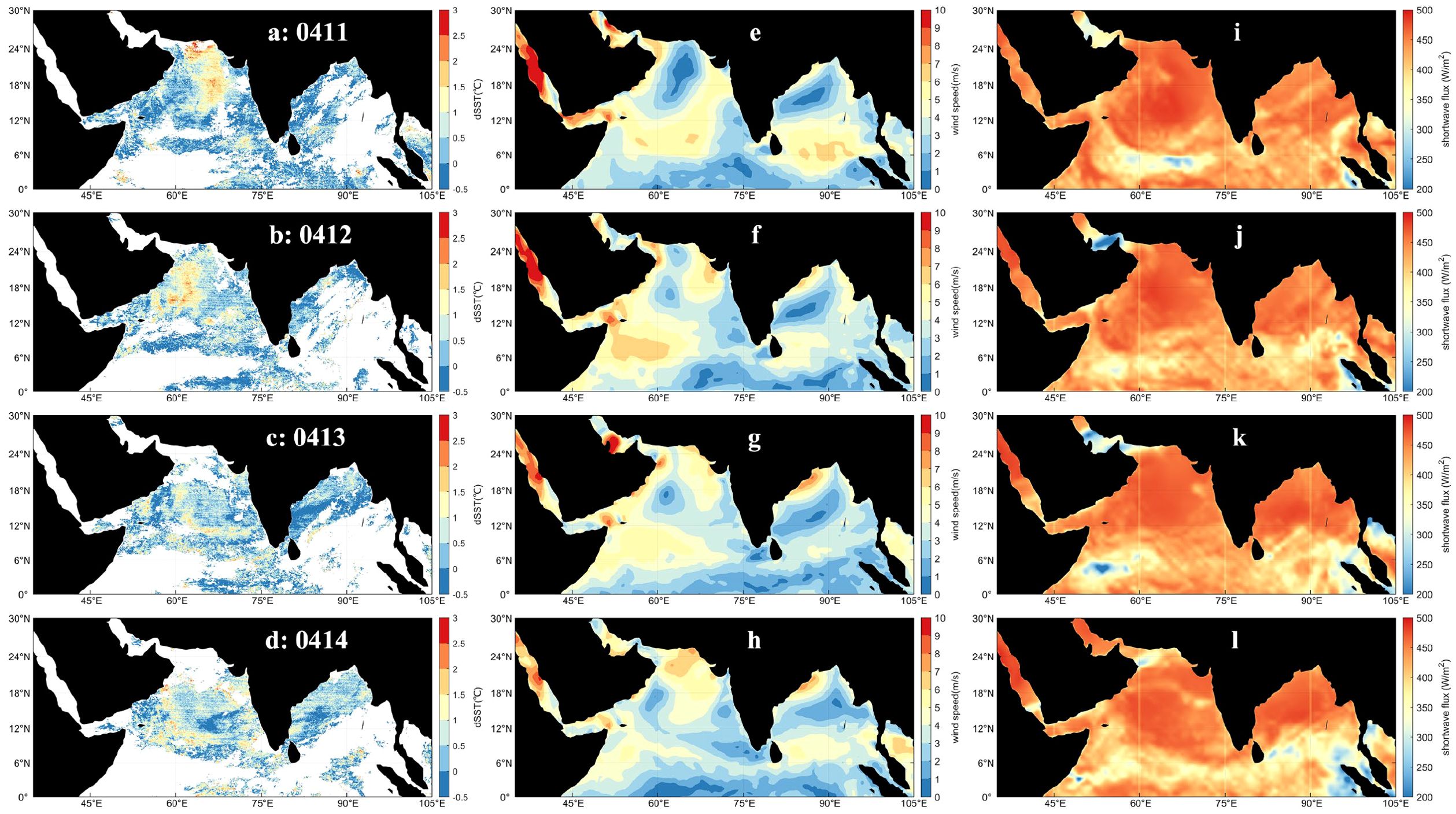
Figure 11. Relationships between dsst (a-d), wind speed (e-h) and shortwave flux (i-l) during a typical diurnal warming event in the North Indian Ocean in 2020.

5.2 Diurnal variation of SST during the MJO in the NIO

The Madden–Julian Oscillation (MJO) is a tropical intraseasonal oscillation (30–90 days cycle) closely tied to ocean–atmosphere interaction (Vialard et al., 2012; Seo et al., 2014). Its active/suppressed phase modulates the magnitude and spatial distribution of diurnal warming through cloudiness, precipitation, and wind. In summary, the diurnally varying of SST enhances the atmospheric wetting process by causing the sea surface temperature to reach higher values during the day. In the tropics, non-precipitating shallow cumulus and diurnally varying cumulonimbus convective clouds continuously transport water vapor to the lower to middle troposphere, gradually making the atmosphere wetter, which prepares the deep convection of the MJO; before the MJO enters the deep convection phase, the temperature change at the ocean surface contributes to the preconditioning of the atmosphere by increasing the latent heat flux (LH) and moist air supply, thus facilitating the initiation and strengthening of the MJO. This humidification is termed the “charge-discharge” mode and constitutes one of the key driving mechanisms for MJO convection (Seo et al., 2014). Therefore, we discuss the relationship between the MJO and the diurnal variation of SST in the North Indian Ocean by matching the active/suppressed phases of the MJO with the corresponding diurnal variation of SST.

The analysis of the RMM indices reveals the presence of one MJO active phase in April and another in May in the North Indian Ocean during 2020, as depicted in Figure 12a. The two MJO active phases are designated as 4/20-4/30 and 5/11-5/21, respectively. A comparative analysis of the amplitude of the RMM indices for these two MJO events indicates that the first one exhibits greater intensity. In accordance with this finding, a quantitative analysis was conducted of the diurnal variation of SST (Figure 12b), wind field (Figure 12c), and solar shortwave flux (Figure 12d) in the North Indian Ocean during April and May of 2020. The weakening of the diurnal warming was captured using the FY-4A SST data in both corresponding MJO events. The number of general diurnal warming events, strong diurnal warming events, and extreme diurnal warming events all show significant decreases during the MJO active phase, and the response time to the MJO events is around 1-2 days. Concurrently, during the MJO active phase, the high wind speed area in the North Indian Ocean exhibits an increasing trend, while the low wind speed area demonstrates a decreasing trend. Additionally, the high shortwave radiation area experiences a decline, while the low shortwave radiation area shows an increase. However, it should be noted that the two MJO events exhibit distinct differences in the magnitude of the wind field changes. Specifically, the first MJO event, being stronger, exhibited a more modest expansion of the high–wind–speed zone and a less pronounced contraction of the low–wind–speed zone compared to the second event. A meticulous examination reveals that the alterations in solar shortwave radiation remain largely congruent between the two MJO events, with no statistically significant disparities observed in the distribution of high and low shortwave radiation regions.

Figure 12

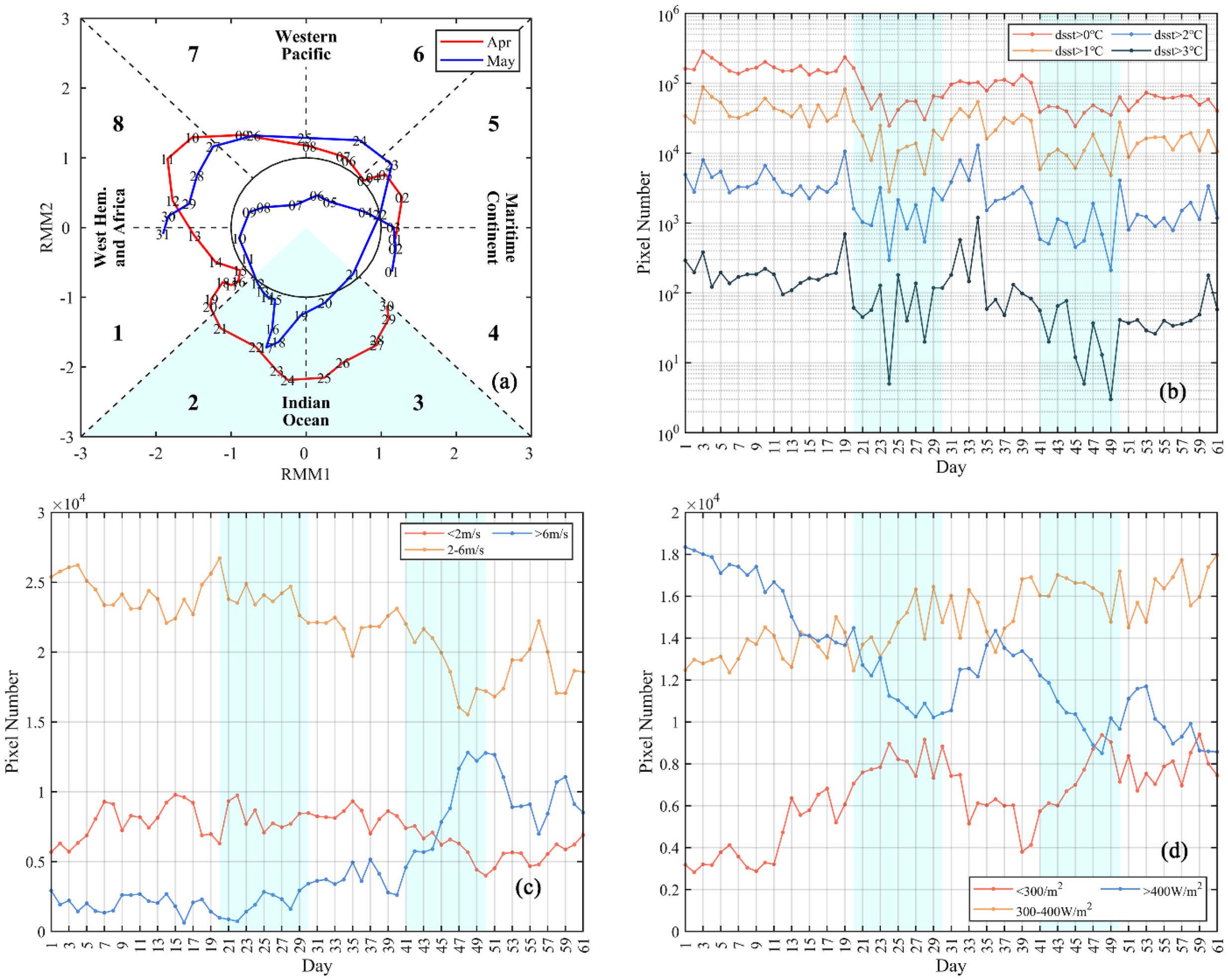
Figure 12. Response of dsst, wind speed, and shortwave flux during two typical MJO events, counted as Day 1 on April 1, 2020: (a) phase space represented by the 2-component MJO index (RMM1, RMM2); (b) changes in the number of pixel points collected for different degrees of diurnal warming in April-May 2020; (c) changes in the number of pixel points collected for different degrees of daily wind speed in April-May 2020; (d) changes in the number of pixel points collected for different degrees of daily shortwave flux in April-May 2020.

In consideration of the developmental pattern of the MJO events, the significant increase of cloudiness during the MJO active phase should be the primary factor affecting the shortwave radiation flux at the sea surface. During the active convective phase of the MJO, the coverage of deep convective clouds expands. Clouds reflect and absorb solar radiation, resulting in an average daily reduction of shortwave radiation flux at the sea surface of 100-200 W/m². Then the decrease in the solar shortwave radiation during the day directly affects the intraday increase in SST. The strong winds and precipitation associated with the MJO active phase may intensify turbulent mixing, deepen the mixing layer, and curtail the intraday increase in SST. It is worth noting that in Section 5.1, we discussed that wind speed is the main influencing factor of the intensity of regional diurnal warming events. However, during the MJO active phase, there is often a significant increase in cloudiness, which reduces shortwave radiation flux and becomes the main influencing factor for the occurrence of diurnal warming events. In the North Indian Ocean, diurnal SST–MJO coupling can be more complex, owing to varied air-sea processes associated with the monsoon climate. In April and May, prior to the onset of the monsoon, a long MJO suppressed phase may result in the occurrence of extreme diurnal warming, leading to the formation of a substantial area of high-SST water (SST > 30°C) in the Arabian Sea. This accelerates the monsoon onset. Conversely, during the monsoon period (June-August), the strong mixing of upper water brought about by the monsoon can substantially suppress the diurnal warming, thereby hindering the formation of a substantial diurnal warming event in the North Indian Ocean waters, irrespective of the MJO suppressed phase. In the post-monsoon period of October-November, the synergistic effect of weak winds with high solar shortwave radiation flux during the MJO suppressed phase leads to the facilitation of a substantial diurnal warming event in the North Indian Ocean.

6 Conclusions

This study examined the diurnal variation of SST in the North Indian Ocean during 2020 using validated FY-4A SST observations, focusing on its relationship with the MJO. Owing to its high temporal resolution, the FY-4A geostationary satellite offers an effective means of observing SST diurnal variation. Through cross-validation against in situ data, the FY-4A full-disk SST exhibits a mean bias of -0.30°C, an absolute bias of 0.77°C, an RSD of 0.35°C, an RMSE of 0.99°C, and a correlation coefficient of 0.99. Within the North Indian Ocean domain, FY-4A SST validations yield a mean bias of -0.33°C, an absolute bias of 0.73°C, an RSD of 0.33°C, an RMSE of 0.94°C, and a correlation coefficient of 0.90. Moreover, the FY-4A SST data demonstrate consistent accuracy across multiple daily intervals, supporting their use in investigating diurnal SST variation in the North Indian Ocean.

Under monsoonal influence, SST diurnal variation in the North Indian Ocean exhibits marked regional and seasonal differences. A year-long statistical analysis of dSST in the North Indian Ocean shows that coastal areas of the Bay of Bengal and the Arabian Sea are prone to diurnal warming, while extreme warming events tend to cluster in lower-latitude areas. Seasonally, March-May (pre-monsoon) and October–November (post-monsoon) exhibits the highest frequency of diurnal warming events. Particularly in March and April, over 80% of the North Indian Ocean experiences at least 15 days of diurnal warming. In July–August (summer monsoon), although the total number of diurnal warming days declines, the proportion of strong and extreme events rises significantly, likely due to intense shortwave radiation during summer. Meanwhile, combined monthly wind speed and solar shortwave flux data from 2020 confirm a negative correlation with dSST for wind speed and a positive correlation for solar radiation, highlighting low wind speed as the principal driver of regional diurnal warming.

The MJO events in the North Indian Ocean correlate strongly with diurnal SST variation, with a response time of about 1–2 days. Comparing the changes in wind speed and shortwave flux during both MJO events reveals that a pronounced reduction in surface shortwave radiation from increased cloudiness plays the dominant role in suppressing diurnal warming. This differs from wind speed, which is the main factor influencing regional diurnal warming. Although reanalysis data are valuable, they may not suffice for fully quantifying the contribution of each factor to diurnal SST variation during MJO events. Buoy data could enhance such quantitative efforts. Furthermore, the North Indian Ocean’s complex atmospheric and oceanic processes, coupled with monsoon conditions, pose notable challenges for monitoring diurnal SST variability. Although high-temporal-resolution geostationary satellite data greatly facilitate research on SST diurnal variation, data availability is still limited by monsoonal winds and the cloud cover associated with MJO events. Hence, integrating geostationary satellite observations, in situ measurements, and numerical model outputs and rigorously confirming their consistency remains crucial for advancing our understanding of SST diurnal variation in the North Indian Ocean, including its mechanisms and broader impacts.

Data availability statement

The original contributions presented in the study are included in the article/supplementary material. Further inquiries can be directed to the corresponding author.

Author contributions

XZ: Writing – original draft, Writing – review & editing. MZ: Writing – review & editing. LZ: Data curation, Formal analysis, Writing – original draft. XS: Data curation, Investigation, Writing – original draft.

Funding

The author(s) declare that financial support was received for the research and/or publication of this article. This work was supported in part by the National Natural Science Foundation of China under Grant 61991454, in part by the National Key Research and Development Program of China under Grant 2023YFC3107605, in part by the Oceanic Interdisciplinary Program of Shanghai Jiao Tong University under Grant SL2022ZD206, and in part by the Scientific Research Fund of Second Institute of Oceanography, MNR under Grant SL2302.

Conflict of interest

The authors declare that the research was conducted in the absence of any commercial or financial relationships that could be construed as a potential conflict of interest.

Generative AI statement

The author(s) declare that no Generative AI was used in the creation of this manuscript.

Publisher’s note

All claims expressed in this article are solely those of the authors and do not necessarily represent those of their affiliated organizations, or those of the publisher, the editors and the reviewers. Any product that may be evaluated in this article, or claim that may be made by its manufacturer, is not guaranteed or endorsed by the publisher.

References

Beggs H., Verein R., Paltoglou G., Kippo H., and Underwood M. (2012). Enhancing ship of opportunity sea surface temperature observations in the Australian region. J. Operational Oceanography 5, 59–73. doi: 10.1080/1755876X.2012.11020132

Crossref Full Text | Google Scholar

Bellenger H. and Duvel J. P. (2012). The event-to-event variability of the boreal winter MJO. Geophysical Res. Lett. 39(8). doi: 10.1029/2012GL051294

Crossref Full Text | Google Scholar

Bernie D. J., Guilyardi E., Madec G., Slingo J. M., Woolnough S. J., and Cole J. (2008). Impact of resolving the diurnal cycle in an ocean-atmosphere GCM. Part 2: A diurnally coupled CGCM. Climate Dynamics 31, 909–925. doi: 10.1007/s00382-008-0429-z

Crossref Full Text | Google Scholar

Castro S. L., Wick G. A., and Buck J. J. (2014). Comparison of diurnal warming estimates from unpumped Argo data and SEVIRI satellite observations. Remote Sens. Environ. 140, 789–799. doi: 10.1016/j.rse.2013.08.042

Crossref Full Text | Google Scholar

Clayson C. A. and Bogdanoff A. S. (2013). The effect of diurnal sea surface temperature warming on climatological air-sea fluxes. J. Climate 26, 2546–2556. doi: 10.1175/JCLI-D-12-00062.1

Crossref Full Text | Google Scholar

Dasgupta P., Roxy M. K., Chattopadhyay R., Naidu C. V., and Metya A. (2021). Interannual variability of the frequency of MJO phases and its association with two types of ENSO. Sci. Rep. 11, 11541–11541. doi: 10.1038/s41598-021-91060-2

PubMed Abstract | Crossref Full Text | Google Scholar

Demott C. A., Klingaman N. P., and Woolnough S. J. (2015). Atmosphere-ocean coupled processes in the Madden-Julian oscillation. Rev. Geophysics 53, 1099–1154. doi: 10.1002/2014RG000478

Crossref Full Text | Google Scholar

De Szoeke S. P., Edson J. B., Marion J. R., Fairall C. W., and Bariteau L. (2015). The MJO and air-sea interaction in TOGA COARE and DYNAMO. J. Climate 28, 597–622. doi: 10.1175/JCLI-D-14-00477.1

Crossref Full Text | Google Scholar

Ditri A., Minnett P., Liu Y., Kilpatrick K., and Kumar A. (2018). The accuracies of himawari-8 and MTSAT-2 sea-surface temperatures in the tropical western pacific ocean. Remote Sens. 10(2), 212. doi: 10.3390/rs10020212

Crossref Full Text | Google Scholar

Donlon C. J., Martin M., Stark J., Roberts-Jones J., Fiedler E., and Wimmer W. (2012). The operational sea surface temperature and sea ice analysis (OSTIA) system. Remote Sens. Environ. 116, 140–158. doi: 10.1016/j.rse.2010.10.017

Crossref Full Text | Google Scholar

Fairall C. W., Bradley E. F., Godfrey J. S., Wick G. A., Edson J. B., and Young G. S. (1996). Cool-skin and warm-layer effects on sea surface temperature. J. Geophysical Research: Oceans 101, 1295–1308. doi: 10.1029/95JC03190

Crossref Full Text | Google Scholar

Gentemann C. L., Fewings M. R., and García-Reyes M. (2017). Satellite sea surface temperatures along the West Coast of the United States during the 2014-2016 northeast Pacific marine heat wave. Geophysical Res. Lett. 44, 312–319. doi: 10.1002/2016GL071039

Crossref Full Text | Google Scholar

Girishkumar M. S., Suprit K., Chiranjivi J., Bhaskar T. V. S., Ravichandran M., Shesu R. V., et al. (2014). Observed oceanic response to tropical cyclone Jal from a moored buoy in the south-western Bay of Bengal. Ocean Dynamics 64, 325–335. doi: 10.1007/s10236-014-0689-6

Crossref Full Text | Google Scholar

He Z., Wu R., and Wang W. (2016). Signals of the South China Sea summer rainfall variability in the Indian Ocean. Climate Dynamics 46, 3181–3195. doi: 10.1007/s00382-015-2760-5

Crossref Full Text | Google Scholar

Hersbach H., Bell B., Berrisford P., Hirahara S., Horányi A., Muñoz-Sabater J., et al. (2020). The ERA5 global reanalysis. Q. J. R. Meteorological Soc. 146, 1999–2049. doi: 10.1002/qj.v146.730

Crossref Full Text | Google Scholar

Hsu J.-Y., Feng M., and Wijffels S. (2021). Observing upper ocean stratification during strong diurnal SST variation events in the suppressed phase of the MJO. Earth Space Sci. Open Arch. 74. doi: 10.1002/essoar.10506155.1

Crossref Full Text | Google Scholar

Ajith Joseph K., Jayaram C., Nair A., George M. S., Balchand A. N., and Pettersson L. H. (2019). Remote Sensing of Upwelling in the Arabian Sea and Adjacent Near-Coastal Regions. In: Barale V. and Gade M. (eds) Remote Sensing of the Asian Seas. Springer, Cham. https://doi.org/10.1007/978-3-319-94067-0_26

Google Scholar

Karagali I. and Høyer J. (2014). Characterisation and quantification of regional diurnal SST cycles from SEVIRI. Ocean Sci. 10, 745–758. doi: 10.5194/os-10-745-2014

Crossref Full Text | Google Scholar

Kawai Y. and Wada A. (2007). Diurnal sea surface temperature variation and its impact on the atmosphere and ocean: A review. J. oceanography 63, 721–744. doi: 10.1007/s10872-007-0063-0

Crossref Full Text | Google Scholar

Kurihara Y., Murakami H., and Kachi M. (2016). Sea surface temperature from the new Japanese geostationary meteorological Himawari-8 satellite. Geophysical Res. Lett. 43, 1234–1240. doi: 10.1002/2015GL067159

Crossref Full Text | Google Scholar

Li L., Liu Y., Zhu Q., Liao K., and Lai X. (2022). Evaluation of nine major satellite soil moisture products in a typical subtropical monsoon region with complex land surface characteristics. Int. Soil Water Conserv. Res. 10, 518–529. doi: 10.1016/j.iswcr.2022.02.003

Crossref Full Text | Google Scholar

Li X., Tang Y., Zhou L., Yao Z., Shen Z., Li J., et al. (2020). Optimal error analysis of MJO prediction associated with uncertainties in sea surface temperature over Indian Ocean. Climate Dynamics 54, 4331–4350. doi: 10.1007/s00382-020-05230-5

Crossref Full Text | Google Scholar

Liu W. H., Cheng J., and Wang Q. (2023). Estimating hourly all-weather land surface temperature from FY-4A/AGRI imagery using the surface energy balance theory. IEEE Trans. Geosci. Remote Sens. 61, 18. doi: 10.1109/TGRS.2023.3254211

Crossref Full Text | Google Scholar

Luo B. and Minnett P. J. (2021). Skin sea surface temperatures from the GOES-16 ABI validated with those of the shipborne M-AERI. IEEE Trans. Geosci. Remote Sens. 59, 9902–9913. doi: 10.1109/TGRS.2021.3054895

Crossref Full Text | Google Scholar

Merchant C. J., Le Borgne P., Marsouin A., and Roquet H. (2008). Optimal estimation of sea surface temperature from split-window observations. Remote Sens. Environ. 112, 2469–2484. doi: 10.1016/j.rse.2007.11.011

Crossref Full Text | Google Scholar

Minnett P. J., Alvera-Azcarate A., Chin T. M., Corlett G. K., Gentemann C. L., Karagali I., et al. (2019). Half a century of satellite remote sensing of sea-surface temperature. Remote Sens. Environ. 233, 111366. doi: 10.1016/j.rse.2019.111366

Crossref Full Text | Google Scholar

Moukomla S. (2015). The estimation of the surface energy balance of the North American Laurentian Great Lakes using satellite remote sensing and MERRA reanalysis (Doctoral dissertation, University of Colorado at Boulder).

Google Scholar

Rayner N., Kawamura H., Reynolds R. W., Mutlow C., Llewellyn-Jones D., Evans R., et al. (2007). The global ocean data assimilation experiment high-resolution sea surface temperature pilot project. Bull. Am. Meteorological Soc. 88, 1197–1214. doi: 10.1175/BAMS-88-8-1197

Crossref Full Text | Google Scholar

Sengupta D. and Ravichandran M. (2001). Oscillations of Bay of Bengal sea surface temperature during the 1998 summer monsoon. Geophysical Res. Lett. 28, 2033–2036. doi: 10.1029/2000GL012548

Crossref Full Text | Google Scholar

Seo H., Subramanian A. C., Miller A. J., and Cavanaugh N. R. (2014). Coupled impacts of the diurnal cycle of sea surface temperature on the madden–julian oscillation. J. Climate 27, 8422–8443. doi: 10.1175/JCLI-D-14-00141.1

Crossref Full Text | Google Scholar

Shenoi S. S. C., Nasnodkar N., Rajesh G., Joseph K. J., Suresh I., and Almeida A. M. (2009). On the diurnal ranges of Sea Surface Temperature (SST) in the north Indian Ocean. J. Earth System Sci. 118, 483–496. doi: 10.1007/s12040-009-0038-1

Crossref Full Text | Google Scholar

Stramma L., Cornillon P., Weller R. A., Price J. F., and Briscoe M. G. (1986). Large diurnal sea-surface temperature variability - satellite and insitu measurements. J. Phys. Oceanography 16, 827–837. doi: 10.1175/1520-0485(1986)016<0827:LDSSTV>2.0.CO;2

Crossref Full Text | Google Scholar

Swapna M., Nayak R. K., Santhoshi T., Sesha Sai M. V. R., and Rajashekhar S. S. (2022). INSAT-3D SST and its diurnal variability assessment using in-situ and MODIS observations. Prog. Oceanography 201, 102739. doi: 10.1016/j.pocean.2022.102739

Crossref Full Text | Google Scholar

Thadathil P., Gopalakrishna V. V., Muraleedharan P. M., Reddy G. V., Araligidad N., and Shenoy S. (2002). Surface layer temperature inversion in the Bay of Bengal. Deep-Sea Res. Part I-Oceanographic Res. Papers 49, 1801–1818. doi: 10.1016/S0967-0637(02)00044-4

Crossref Full Text | Google Scholar

Thadathil P., Suresh I., Gautham S., Kumar S. P., Lengaigne M., Rao R. R., et al. (2016). Surface layer temperature inversion in the Bay of Bengal: Main characteristics and related mechanisms. J. Geophysical Research-Oceans 121, 5682–5696. doi: 10.1002/2016JC011674

Crossref Full Text | Google Scholar

Tu Q. and Hao Z. (2020). Validation of sea surface temperature derived from himawari-8 by JAXA. IEEE J. Selected Topics Appl. Earth Observations Remote Sens. 13, 448–459. doi: 10.1109/JSTARS.4609443

Crossref Full Text | Google Scholar

Vialard J., Jayakumar A., Gnanaseelan C., Lengaigne M., Sengupta D., and Goswami B. N. (2012). Processes of 30-90 days sea surface temperature variability in the northern Indian Ocean during boreal summer. Climate Dynamics 38, 1901–1916. doi: 10.1007/s00382-011-1015-3

Crossref Full Text | Google Scholar

Wheeler M. C. and Hendon H. H. (2004). An all-season real-time multivariate MJO index: Development of an index for monitoring and prediction. Monthly Weather Rev. 132, 1917–1932. doi: 10.1175/1520-0493(2004)132<1917:AARMMI>2.0.CO;2

Crossref Full Text | Google Scholar

Wick G. A. and Castro S. L. (2020). Assessment of extreme diurnal warming in operational geosynchronous satellite sea surface temperature products. Remote Sens. 12(22), 3771. doi: 10.3390/rs12223771

Crossref Full Text | Google Scholar

Wirasatriya A., Hosoda K., Setiawan J. D., and Susanto R. D. (2020). Variability of diurnal sea surface temperature during short term and high SST event in the western equatorial pacific as revealed by satellite data. Remote Sens. 12(19), 3230. doi: 10.3390/rs12193230

Crossref Full Text | Google Scholar

Woolnough S. J., Slingo J. M., and Hoskins B. J. (2000). The relationship between convection and sea surface temperature on intraseasonal timescales. J. Climate 13, 2086–2104. doi: 10.1175/1520-0442(2000)013<2086:TRBCAS>2.0.CO;2

Crossref Full Text | Google Scholar

Xu F. and Ignatov A. (2014). In situ SST quality monitor (iQuam). J. Atmospheric Oceanic Technol. 31, 164–180. doi: 10.1175/JTECH-D-13-00121.1

Crossref Full Text | Google Scholar

Xu Y., Yu L., Peng D., Zhao J., Cheng Y., Liu X., et al. (2020). Annual 30-m land use/land cover maps of China for 1980-2015 from the integration of AVHRR, MODIS and Landsat data using the BFAST algorithm. Sci. China-Earth Sci. 63, 1390–1407. doi: 10.1007/s11430-019-9606-4

Crossref Full Text | Google Scholar

Ye X., Liu J., Lin M., Ding J., Zou B., and Song Q. (2021). Sea surface temperatures derived from COCTS onboard the HY-1C satellite. IEEE J. Selected Topics Appl. Earth Observations Remote Sens. 14, 1038–1047. doi: 10.1109/JSTARS.4609443

Crossref Full Text | Google Scholar

Yu F., Wu X., Yoo H., Qian H., Shao X., Wang Z., et al. (2021). Radiometric calibration accuracy and stability of GOES-16 ABI Infrared radiance. J. Appl. Remote Sens. 15(4), 048504. doi: 10.1117/1.JRS.15.048504

Crossref Full Text | Google Scholar

Zhang H., Beggs H., Majewski L., Wang X. H., and Kiss A. (2016a). Investigating sea surface temperature diurnal variation over the Tropical Warm Pool using MTSAT-1R data. Remote Sens. Environ. 183, 1–12. doi: 10.1016/j.rse.2016.05.002

Crossref Full Text | Google Scholar

Zhang H., Beggs H., Wang X. H., Kiss A. E., and Griffin C. (2016b). Seasonal patterns of SST diurnal variation over the Tropical Warm Pool region. J. Geophysical Research: Oceans 121, 8077–8094. doi: 10.1002/2016JC012210

Crossref Full Text | Google Scholar